

1. Introduction
Over the past century and a half, real per capita GDP in the U.S. has grown at an average annual rate of about 2%. Historical growth accounting attributes this performance primarily to capital deepening (see, e.g., Solow, Reference Solow1957), increased years of schooling (see, e.g., Barro and Lee, Reference Barro and Lee2015), and improved allocation of scarce resources (see, e.g., Restuccia and Rogerson, Reference Restuccia and Rogerson2017). However, sustained long-run growth also requires technological progress, where research generates innovative ideas that lead to new product varieties (see, e.g., Romer, Reference Romer1990; Jones, Reference Jones1995) and/or higher product quality (see, e.g., Aghion and Howitt, Reference Aghion and Howitt1992; Aghion et al. Reference Aghion, Akcigit, Howitt, Aghion, Akcigit and Howitt2014).Footnote 1
Complementing growth accounting, the literature has examined the structural forces shaping these drivers. Key influences include physical infrastructure, market efficiency, education systems, trade openness, and institutional frameworks governing interactions among firms, individuals, and policymakers (see reviews in Aghion and Howitt, Reference Aghion and Howitt2009; Acemoglu, Reference Acemoglu2009; Sala-i-Martin, Reference Sala-i-Martin and Sala-i-Martin2010; and Aghion and Durlauf, Reference Aghion and Durlauf2005, Reference Aghion and Durlauf2014).
This paper combines and extends features from several growth models to assess quantitatively how permanent structural policy changes, or reforms, affect these underlying forces and, in turn, long-term growth and welfare in the U.S. economy. Following the related literature, we adopt a broad interpretation of policy and focus on reforms that improve market functioning, fiscal policy composition, and institutional quality.Footnote 2 Specifically, we examine three reforms: (i) reducing regulatory costs faced by firms, (ii) increasing public investment financed by lower transfers, and (iii) improving the legal-political framework to curb rent-seeking related to the public budget.
We focus on permanent changes because our interest lies in long-term outcomes rather than short-run business cycles. To analyse these reforms, we build on the Romer–Jones model of endogenous growth, distinguishing among final-good firms, intermediate-goods firms, and research firms, the latter producing ideas that enhance productivity by creating new product varieties. We enrich this framework in three ways. First, we incorporate human capital accumulation à la Lucas (Reference Lucas1988), given its role in idea creation.Footnote 3 Second, we allow government policies to influence resource allocation by including productivity-enhancing public investment and public consumption. Third, we model resource misallocation through rent-seeking contests for fiscal favours, which divert labour from productive activities.
Within this unified general equilibrium setup, ideas and human capital drive long-run endogenous per capita growth, while transitional dynamics also reflect accumulation of labour, physical capital, and public capital. The model is calibrated using U.S. data dating back to 1925.
Our quantitative analysis, calibrated to U.S. data, shows that the economy’s baseline balanced growth path (BGP) features an annual per capita growth rate of about 2%, consistent with historical averages. Then, structural reforms can meaningfully alter this trajectory, but their effects differ in magnitude and character. Eliminating regulatory costs delivers only modest growth gains ( $\approx$
0.46%) because the implicit “tax” on labour is small.Footnote
4
Yet it produces immediate efficiency gains and welfare improvements of roughly 4%, with virtually no short-run adjustment costs. By contrast, increasing public investment by one percentage point (1 ppt) raises long-run growth by nearly 3% and welfare by 3.5%, while, larger than 1 ppt increases can yield more-than-proportional benefits. However, these gains come with short-run consumption sacrifices and slower adjustment. Institutional reform through eliminating rent-seeking improves efficiency and welfare (
$\approx$
0.46%) because the implicit “tax” on labour is small.Footnote
4
Yet it produces immediate efficiency gains and welfare improvements of roughly 4%, with virtually no short-run adjustment costs. By contrast, increasing public investment by one percentage point (1 ppt) raises long-run growth by nearly 3% and welfare by 3.5%, while, larger than 1 ppt increases can yield more-than-proportional benefits. However, these gains come with short-run consumption sacrifices and slower adjustment. Institutional reform through eliminating rent-seeking improves efficiency and welfare ( $\approx$
3.1%), while increasing leisure, a distinctive advantage over other reforms, but its growth impact (
$\approx$
3.1%), while increasing leisure, a distinctive advantage over other reforms, but its growth impact ( $\approx$
1.2%) remains smaller than that of public investment. Taken together, these results highlight that while all three reforms enhance welfare, fiscal and institutional changes operate through different channels: public investment is the most powerful lever for growth, regulatory simplification offers quick welfare gains, and curbing rent-seeking improves efficiency without reducing leisure.
$\approx$
1.2%) remains smaller than that of public investment. Taken together, these results highlight that while all three reforms enhance welfare, fiscal and institutional changes operate through different channels: public investment is the most powerful lever for growth, regulatory simplification offers quick welfare gains, and curbing rent-seeking improves efficiency without reducing leisure.
We structure the paper as follows: Section 2 presents the model, Section 3 covers the calibration, Section 4 the quantitative analysis, and Section 5 the conclusions.
2. Model
Our decentralised economic model builds on the work of Lucas (Reference Lucas1988), Romer (Reference Romer1990), Jones (Reference Jones1995), and Gross and Klein (Reference Gross and Klein2022). It includes firms, households, and a government.
Firms are categorised into three types: final goods producers, intermediate goods producers, and research firms, following the Romer-Jones framework. All firms are treated symmetrically, optimising their input choices to maximise the discounted present value of profits. Additionally, firms incur regulatory costs that use real resources and may engage in rent-seeking behaviour to capture state resources.
Households are identical, and, in addition to making consumption and savings decisions, they allocate their time between leisure, work, and education. Education increases human capital, as Lucas’s model suggests.
The government controls several fiscal policy instruments that influence incentives, factor accumulation, and macroeconomic growth. On the tax side, it levies taxes on firms’ profits, personal income, and consumption. On the spending side, the government allocates resources to public consumption, public investment, and income transfers to households. Public investment improves public infrastructure, which in turn boosts both firm productivity and household human capital.
Regulatory costs represent real resource expenditures associated with running a firm, often arising from product-market regulations (Blanchard and Giavazzi, Reference Blanchard and Giavazzi2003; Fang and Rogerson, Reference Fang and Rogerson2011; Trebbi and Zhang, Reference Trebbi and Zhang2022). For example, firms must allocate labour resources to activities such as filing reports, attending meetings, and obtaining approvals (Fang and Rogerson, Reference Fang and Rogerson2011). These costs are modelled as a proportion of each firm’s total wage bill, allocated to regulatory compliance.
In terms of core institutions and rent-seeking, firms compete in a Tullockian fashion for extra fiscal favours, such as additional government transfers, that boost their profits. This competition leads to a misallocation of resources at the societal level, as firms allocate part of their workforce to rent-seeking rather than productive activities. It also reduces the share of public spending dedicated to productivity- and utility-enhancing public goods and services.
Finally, from a technical perspective, it is important to note that specific functional forms are needed in an endogenously growing economy to ensure a stationary, detrended transformation in equilibrium (see Jones et al., Reference Jones, Manuelli and Siu2005a; Herrendorf et al., Reference Herrendorf, Rogerson, Valentinyi, Herrendorf, Rogerson and Valentinyi2014).
2.1 Firms
We start by building upon the Romer-Jones three-sector model, in which productivity growth arises from an expanding variety of intermediate inputs or machines that use ideas or blueprints.Footnote
5
Identical final-good firms produce a single final good, which is used for consumption, investment, public goods and services as well as any resource-type costs. These firms hire labour from households and rent a variety of differentiated intermediate inputs from intermediate-goods firms. The latter hire labour, invest in physical capital, and, to operate, they need to purchase a blueprint or an idea from research firms. Research firms hire researchers to produce blueprints or ideas. All three types of firms maximise their profits explicitly, which generalises the related literature. Following the same literature, we will assume that every new blueprint adds one more variety of intermediate goods and that each research firm makes one blueprint. In equilibrium, the number of final good firms, $N_{f,t}$
, will be assumed, for notational simplicity, to equal the number of intermediate goods firms,
$N_{f,t}$
, will be assumed, for notational simplicity, to equal the number of intermediate goods firms, $N_{i,t}$
. This number will be set equal to the number of research firms and blueprints,
$N_{i,t}$
. This number will be set equal to the number of research firms and blueprints, $N_{b,t}$
, where the latter is endogenously determined as in the Romer-Jones setup. Finally, as said above, all firms benefit from public infrastructure, incur regulatory costs, and can rent-seek from state coffers.
$N_{b,t}$
, where the latter is endogenously determined as in the Romer-Jones setup. Finally, as said above, all firms benefit from public infrastructure, incur regulatory costs, and can rent-seek from state coffers.
2.1.1 Firms in the final-good sector
At each $t$
, there are
$t$
, there are $f=1,2,\ldots N_{f,t}$
identical final-good producers. Each
$f=1,2,\ldots N_{f,t}$
identical final-good producers. Each $f$
produces
$f$
produces $y_{f,t}$
using the technology:
$y_{f,t}$
using the technology:
 \begin{align} y_{f,t}=A_{f,t}\Big(l_{f,t}^{w}\Big)^{a}\left( \sum\nolimits _{i=1}^{N_{i,t}}x_{f,i,t}^{1-\alpha }\right) \text{,} \end{align}
where $l_{f,t}^{w}$
and
$l_{f,t}^{w}$
and $x_{f,i,t}$
are, respectively, the units of labour input and the amount of each intermediate input or machine of variety
$x_{f,i,t}$
are, respectively, the units of labour input and the amount of each intermediate input or machine of variety $i=1,2,\ldots ,N_{i,t}$
used by each firm
$i=1,2,\ldots ,N_{i,t}$
used by each firm $f$
in production, and
$f$
in production, and $0\lt \alpha \lt 1$
is a technology parameter. This production function follows the literature cited above and implies that product varieties, and hence ideas, are labour-augmenting.Footnote
6
Further, note that we assume:
$0\lt \alpha \lt 1$
is a technology parameter. This production function follows the literature cited above and implies that product varieties, and hence ideas, are labour-augmenting.Footnote
6
Further, note that we assume:
 \begin{align} A_{f,t}\equiv A_{f}\left ( \widetilde {k}_{t}^{\,g}\right ) ^{\phi }\text{,} \end{align}
where $A_{f}\gt 0$
is a scale parameter;
$A_{f}\gt 0$
is a scale parameter; $\widetilde {k}_{t}^{\,g}$
is per firm productivity-enhancing public capital expressed in efficiency units;Footnote
7
and the parameter
$\widetilde {k}_{t}^{\,g}$
is per firm productivity-enhancing public capital expressed in efficiency units;Footnote
7
and the parameter $0\lt \phi \lt 1$
measures the productivity of
$0\lt \phi \lt 1$
measures the productivity of $\widetilde {k}_{t}^{\,g}$
.
$\widetilde {k}_{t}^{\,g}$
.
In each period $t$
, each firm
$t$
, each firm $f$
maximises its after-tax gross profit defined as:
$f$
maximises its after-tax gross profit defined as:
 \begin{align} \pi _{f,t} \equiv &\ \Big(1-\tau _{t}^{\,f}\Big)\Big( y_{f,t}-w_{t}(l_{f,t}^{w}+l_{f,t}^{r})-\sum\nolimits _{i=1}^{N_{i,t}}p_{i,t}x_{f,i,t} \Big) +\left ( \frac {l_{f,t}^{r}}{L_{t}^{r}}\right ) G_{t}^{\,p}-r_{c}w_{t}\big(l_{f,t}^{w}+l_{f,t}^{r}\big)\text{,} \end{align}
where $p_{i,t}$
is the price of intermediate input of variety
$p_{i,t}$
is the price of intermediate input of variety $i$
relative to the single final good price or the numeraire;
$i$
relative to the single final good price or the numeraire; $ l_{f,t}^{r}$
is the units of labour input used for rent-seeking activities by each final good firm
$ l_{f,t}^{r}$
is the units of labour input used for rent-seeking activities by each final good firm $f$
(e.g. lobbying, etc.), while
$f$
(e.g. lobbying, etc.), while $ L_{t}^{r}$
is the total amount of these inputs used by all firms in the economy;Footnote
8
$ L_{t}^{r}$
is the total amount of these inputs used by all firms in the economy;Footnote
8 $G_{t}^{\,p}$
denotes the contestable pie (defined below);
$G_{t}^{\,p}$
denotes the contestable pie (defined below); $r_{c}\geq 0$
is a policy parameter measuring the fraction of the firm’s total wage bill spent on regulatory tasks (see also e.g. Trebbi and Zhang (Reference Trebbi and Zhang2022)); and
$r_{c}\geq 0$
is a policy parameter measuring the fraction of the firm’s total wage bill spent on regulatory tasks (see also e.g. Trebbi and Zhang (Reference Trebbi and Zhang2022)); and $0\leq \tau _{t}^{\,f}$ $\lt 1$
is the corporate tax rate on firms’ gross profits. Notice that
$\lt 1$
is the corporate tax rate on firms’ gross profits. Notice that $\frac { l_{f,t}^{r}}{L_{t}^{r}}$
is the classic rent-seeking technology or redistributive contest introduced by Tullock (Reference Tullock1967) and used, for example, by Murphy et al. (Reference Murphy, Shleifer and Vishny1991), Esteban and Ray (Reference Esteban and Ray2011) and Angelopoulos et al. (Reference Angelopoulos, Angelopoulos, Lazarakis and Philippopoulos2021).Footnote
9
$\frac { l_{f,t}^{r}}{L_{t}^{r}}$
is the classic rent-seeking technology or redistributive contest introduced by Tullock (Reference Tullock1967) and used, for example, by Murphy et al. (Reference Murphy, Shleifer and Vishny1991), Esteban and Ray (Reference Esteban and Ray2011) and Angelopoulos et al. (Reference Angelopoulos, Angelopoulos, Lazarakis and Philippopoulos2021).Footnote
9
First-order conditions Final good firms act competitively. The first-order conditions for $ l_{f,t}^{w}$
,
$ l_{f,t}^{w}$
, $l_{f,t}^{r}$
and
$l_{f,t}^{r}$
and $x_{f,i,t}$
, giving the demand for the two types of labour activity (i.e. productive work and rent-seeking) and for each intermediate input
$x_{f,i,t}$
, giving the demand for the two types of labour activity (i.e. productive work and rent-seeking) and for each intermediate input $i$
, respectively, are:
$i$
, respectively, are:
 \begin{align} \Big(1-\tau _{t}^{\,f}+r_{c}\Big)w_{t}=\big(1-\tau _{t}^{\,f}\big)\frac {\alpha y_{f,t}}{ l_{f,t}^{w}}\text{,} \end{align}
 \begin{align} \Big(1-\tau _{t}^{\,f}+r_{c}\Big)w_{t}=\left ( \frac {1}{L_{t}^{r}}\right ) G_{t}^{\,p} \text{,} \end{align}
 \begin{align} p_{i,t}=\frac {\left ( 1-\alpha \right ) y_{f,t}\left ( x_{f,i,t}\right ) ^{-\alpha }}{\sum _{i=1}^{N_{i,t}}x_{f,i,t}^{1-\alpha }}\text{.} \end{align}
Thus, eqs. (4)–(6) characterise the final-good firm’s optimal input choices by equating marginal benefits to marginal costs. Equation (4) states that productive labour is hired up to the point where its after-tax marginal product equals the effective marginal cost of labour, which includes both the wage and regulatory burden. Equation (5) shows that the firm allocates labour to rent-seeking until the expected marginal gain from increasing its share in the Tullock contest for the government’s contestable resources equals the same effective labour cost. Finally, eq. (6) gives the demand for each intermediate input by equating its price to its marginal contribution to final output, reflecting standard diminishing returns across differentiated varieties. Together, these conditions capture how firms optimally divide labour between productive and unproductive activities and choose intermediate inputs within a competitive final-goods sector subject to taxes and regulatory costs.
2.1.2 Firms in the intermediate-goods sector
At each $t$
, there are
$t$
, there are $i=1,2,\ldots N_{i,t}$
intermediate-goods producers, one for each input of variety
$i=1,2,\ldots N_{i,t}$
intermediate-goods producers, one for each input of variety $i$
. Each
$i$
. Each $i$
produces
$i$
produces $x_{i,t}$
using the technology:
$x_{i,t}$
using the technology:
 \begin{align} x_{i,t}=A_{i,t}\left ( N_{b,t}l_{i,t}^{w}\right ) ^{\alpha }k_{i,t}^{1-\alpha }\text{,} \end{align}
where $l_{i,t}^{w}$
and
$l_{i,t}^{w}$
and $k_{i,t}$
are, respectively, the labour and capital inputs used by firm
$k_{i,t}$
are, respectively, the labour and capital inputs used by firm $i$
in production, and
$i$
in production, and $N_{b,t}$
is the labour-augmenting number of blueprints in the economy.Footnote
10
Further note that, as in (2) above, we assume:
$N_{b,t}$
is the labour-augmenting number of blueprints in the economy.Footnote
10
Further note that, as in (2) above, we assume:
 \begin{align} A_{i,t}\equiv A_{i}\left ( \widetilde {k}_{t}^{\,g}\right ) ^{\phi }\text{,} \end{align}
where $A_{i}\gt 0$
is a scale parameter.Footnote
11
$A_{i}\gt 0$
is a scale parameter.Footnote
11
The motion of private capital used by each firm $i$
is:
$i$
is:
 \begin{align} k_{i,t+1}=(1-\delta )k_{i,t}+in_{i,t}\text{,} \end{align}
where $0\leq \delta \leq 1$
is the depreciation rate, and
$0\leq \delta \leq 1$
is the depreciation rate, and $in_{i,t}$
is firm
$in_{i,t}$
is firm $i$
’s investment in physical capital.
$i$
’s investment in physical capital.
Each $i$
purchases a blueprint to operate, which works like a fixed cost within each period. As in Gross and Klein (Reference Gross and Klein2022), we assume that patents or blueprints last for one period only (hence their price,
$i$
purchases a blueprint to operate, which works like a fixed cost within each period. As in Gross and Klein (Reference Gross and Klein2022), we assume that patents or blueprints last for one period only (hence their price, $q_{t}$
, enters the flow payoff in each period), which, in the calibration below, will correspond to 20 years.Footnote
12
Therefore, each
$q_{t}$
, enters the flow payoff in each period), which, in the calibration below, will correspond to 20 years.Footnote
12
Therefore, each $i$
maximises the discounted value of its after-tax net cash flows, or its value, defined as:
$i$
maximises the discounted value of its after-tax net cash flows, or its value, defined as:
 \begin{align} &\sum \limits _{t=0}^{\infty }\beta _{i,t}\pi _{i,t}\nonumber\\&\equiv \sum \limits _{t=0}^{\infty }\beta _{i,t}\left [ \big(1-\tau _{t}^{\,f}\big)[p_{i,t}x_{i,t}-w_{t}(l_{i,t}^{w}+l_{i,t}^{r})-q_{t}] - in_{i,t}+\left ( \frac {l_{i,t}^{r}}{L_{t}^{r}}\right ) G_{t}^{\,p}-r_{c}w_{t}(l_{i,t}^{w}+l_{i,t}^{r})\right ] , \end{align}
where $q_{t}$
is the price of the blueprint purchased from the research sector;
$q_{t}$
is the price of the blueprint purchased from the research sector; $l_{i,t}^{r}$
is the labour input used for rent-seeking activities by each intermediate good firm
$l_{i,t}^{r}$
is the labour input used for rent-seeking activities by each intermediate good firm $i$
; and
$i$
; and $\beta _{i,t}$
is the firm’s time discount factor (defined below). The rest of the variables are as in the final good firm’s problem above.
$\beta _{i,t}$
is the firm’s time discount factor (defined below). The rest of the variables are as in the final good firm’s problem above.
First-order conditions Each intermediate-goods firm $i$
acts monopolistically in its product market by taking into account its product’s demand function, eq. (6).Footnote
13
The first-order conditions for
$i$
acts monopolistically in its product market by taking into account its product’s demand function, eq. (6).Footnote
13
The first-order conditions for $l_{i,t}^{w}$
,
$l_{i,t}^{w}$
, $l_{i,t}^{r}$
and
$l_{i,t}^{r}$
and $k_{i,t+1}$
, giving the demand for the two types of labour activity and for physical capital, respectively, are:
$k_{i,t+1}$
, giving the demand for the two types of labour activity and for physical capital, respectively, are:
 \begin{align} \Big(1-\tau _{t}^{\,f}+r_{c}\Big)w_{t}=\frac {\big(1-\tau _{t}^{\,f}\big)(1-\alpha )^{2}y_{f,t}\left ( x_{i,t}\right ) ^{-\alpha }}{\frac {1}{N_{f,t}} \sum _{i=1}^{N_{i,t}}x_{i,t}^{1-\alpha }}\frac {\alpha x_{i,t}}{l_{i,t}}\text{, } \end{align}
 \begin{align} \Big(1-\tau _{t}^{\,f}+r_{c}\Big)w_{t}=\left ( \frac {1}{L_{t}^{r}}\right ) G_{t}^{\,p} \text{,} \end{align}
 \begin{align} 1=\beta _{i,1}\left [ 1-\delta +\frac {(1-\tau _{t+1}^{\,f})(1-\alpha )^{2}y_{f,t+1}(x_{i,t+1})^{-\alpha }}{\frac {1}{N_{f,t+1}} \sum _{i=1}^{N_{i,t+1}}x_{i,t+1}^{1-\alpha }}\frac {(1-\alpha )x_{i,t+1}}{ k_{i,t+1}}\right ]. \end{align}
Following the Romer-Jones literature, we assume that the research firm that produces and sells the blueprint sets its price, $q_{t}$
, to extract the intermediate good firm’s monopoly profit (see e.g. Jones (Reference Jones1995, p. 781)), so that we have from eq. (10) above:Footnote
14
$q_{t}$
, to extract the intermediate good firm’s monopoly profit (see e.g. Jones (Reference Jones1995, p. 781)), so that we have from eq. (10) above:Footnote
14
 \begin{align} q_{t}=\frac {\big(1-\tau _{t}^{\,f}\big)[p_{i,t}x_{i,t}-w_{t}(l_{i,t}^{w}+l_{i,t}^{r})]-in_{i,t}+\left ( \frac {l_{i,t}^{r}}{L_{t}^{r}}\right ) G_{t}^{\,p}-r_{c}w_{t}(l_{i,t}^{w}+l_{i,t}^{r})}{\big(1-\tau _{t}^{\,f}\big)}\text{.} \end{align}
Thus, eqs. (11)–(14) describe the optimal input choices of each intermediate-goods producer by equating marginal benefits to marginal costs. Equation (11) shows that productive labour is hired until its full marginal cost - including the wage and regulatory burden - equals its after-tax marginal revenue product, which incorporates both diminishing returns and the firm’s monopoly markup. Equation (12) states that rent-seeking labour is used up to the point where the expected marginal gain from increasing the firm’s share in the Tullock contest for government resources equals the same effective labour cost. Equation (13) is the Euler condition for physical capital, requiring that the marginal cost of investing today equals the discounted expected after-tax return from the additional capital tomorrow, reflecting both depreciation and its contribution to monopoly revenue. Finally, eq. (14) determines the blueprint price as the value that allows the research sector to extract the full flow monopoly profit of intermediate-goods firms, ensuring zero economic profit and linking innovation incentives to the profitability of operating a differentiated variety.
2.1.3 Firms in the research sector
At each $t$
, there are
$t$
, there are $b=1,2,\ldots N_{b,t}$
identical research firms whose number is endogenously determined. We assume that each
$b=1,2,\ldots N_{b,t}$
identical research firms whose number is endogenously determined. We assume that each $b$
produces one blueprint or idea in each period where, as said above, the period will correspond to 20 years as in Gross and Klein (Reference Gross and Klein2022). In other words, as in the Romer-Jones literature, since one research firm generates one blueprint, the number of total blueprints coincides with the number of research firms. Following the same literature, this number is assumed to evolve over time as:
$b$
produces one blueprint or idea in each period where, as said above, the period will correspond to 20 years as in Gross and Klein (Reference Gross and Klein2022). In other words, as in the Romer-Jones literature, since one research firm generates one blueprint, the number of total blueprints coincides with the number of research firms. Following the same literature, this number is assumed to evolve over time as:
 \begin{align} N_{b,t+1}=\left ( 1-\delta ^{n_{b}}\right ) N_{b,t}+M_{t}N_{b,t}l_{b,t}^{w}H_{t}\left ( N_{b,t}\right ) ^{\mu }\text{,} \end{align}
where $l_{b,t}^{w}$
is the units of labour input used by each of the
$l_{b,t}^{w}$
is the units of labour input used by each of the $b$
research firms for the production of the blueprint so that
$b$
research firms for the production of the blueprint so that $N_{b,t}l_{b,t}^{w}$
is the total labour input used for research by the whole sector;
$N_{b,t}l_{b,t}^{w}$
is the total labour input used for research by the whole sector; $H_{t}$
is the economy’s total human capital stock acting as an externality in the generation of ideas;
$H_{t}$
is the economy’s total human capital stock acting as an externality in the generation of ideas; $0\leq \delta ^{n_{b}}\leq 1$
is the depreciation rate which, since blueprints last for one period (corresponding to 20 years) will be set at 1 in the calibration section; and the power coefficient,
$0\leq \delta ^{n_{b}}\leq 1$
is the depreciation rate which, since blueprints last for one period (corresponding to 20 years) will be set at 1 in the calibration section; and the power coefficient, $\mu \lt 1$
, is a technology parameter whose range of values, as argued by, e.g. Jones (Reference Jones2019, Reference Jones2022a), captures the fact that ”ideas are becoming harder to find”.Footnote
15
Further note that, as in (2) and (8) above, we assume:
$\mu \lt 1$
, is a technology parameter whose range of values, as argued by, e.g. Jones (Reference Jones2019, Reference Jones2022a), captures the fact that ”ideas are becoming harder to find”.Footnote
15
Further note that, as in (2) and (8) above, we assume:
 \begin{align} M_{t}\equiv M\left ( \widetilde {k}_{t}^{\,g}\right ) ^{\phi }\text{,} \end{align}
where $M\gt 0$
is a scale parameter.
$M\gt 0$
is a scale parameter.
Each firm $b$
maximises the discounted present value of its after-tax gross profits defined as:Footnote
16
$b$
maximises the discounted present value of its after-tax gross profits defined as:Footnote
16
 \begin{align} \sum \limits _{t=0}^{\infty }\beta _{b,t}\pi _{b,t}\equiv \sum \limits _{t=0}^{\infty }\beta _{b,t}\left [\left(1-\tau _{t}^{\,f}\right)\big[q_{t}-w_{t}\big(l_{b,t}^{w}+l_{b,t}^{r}\big)\big]+\left ( \frac {l_{b,t}^{r}}{ L_{t}^{r}}\right ) G_{t}^{\,p}-r_{c}w_{t}\big(l_{b,t}^{w}+l_{b,t}^{r}\big)\right] , \end{align}
where $l_{b,t}^{r}$
is the labour input used by each of the
$l_{b,t}^{r}$
is the labour input used by each of the $b$
research firms for rent-seeking activities; and
$b$
research firms for rent-seeking activities; and $\beta _{b,t}=\beta _{i,t}$
(defined below). Notice that each firm’s revenue is the price of the blueprint,
$\beta _{b,t}=\beta _{i,t}$
(defined below). Notice that each firm’s revenue is the price of the blueprint, $q_{t}$
, times the number of blueprints produced and sold by this firm, where the latter has been set at
$q_{t}$
, times the number of blueprints produced and sold by this firm, where the latter has been set at $1$
as said above. The rest of the variables are as in the final and intermediate good firms’ problems above.
$1$
as said above. The rest of the variables are as in the final and intermediate good firms’ problems above.
First-order conditions Using the law of motion of ideas into the profit function,Footnote
17
the first-order conditions for $l_{b,t}^{w}$
and
$l_{b,t}^{w}$
and $l_{b,t}^{r}$
or each firm
$l_{b,t}^{r}$
or each firm $b$
’s demand for the two types of labour activity are respectively:
$b$
’s demand for the two types of labour activity are respectively:
 \begin{align} \left(1-\tau _{t}^{\,f}+r_{c}\right)w_{t}=\beta _{b,1}\left ( 1-\tau _{t+1}^{\,f}\right ) q_{t+1}\frac {N_{b,t}}{N_{b,t+1}}M_{t}H_{t}\left ( N_{b,t}\right ) ^{\mu }, \end{align}
 \begin{align} \big(1-\tau _{t}^{\,f}+r_{c}\big)w_{t}=\left ( \frac {1}{L_{t}^{r}}\right ) G_{t}^{\,p}. \end{align}
Thus, eqs. (18) and (19) describe the research firm’s optimal allocation of labour between productive idea creation and rent-seeking. Equation (18) states that productive research labour is hired up to the point where its effective marginal cost, the wage inclusive of regulatory burdens, equals the discounted marginal benefit from generating an additional blueprint that can be sold in the next period. Equation (19) shows that rent-seeking labour is used until its marginal cost equals the expected marginal gain from increasing the firm’s share in the Tullock contest for the government’s contestable resources. These conditions highlight how research firms balance forward-looking innovation incentives with purely redistributive rent-seeking motives when deciding how to allocate labour.
2.2 Households
Households consume, work and save in the form of government bonds. They also own the firms and so receive their dividends. In addition to time allocated to work and leisure, they allocate time to education, which augments their human capital a la Lucas (Reference Lucas1988).
There are $h=1,2,\ldots ,N_{t}$
identical households. Each
$h=1,2,\ldots ,N_{t}$
identical households. Each $h$
maximises lifetime utility defined as:
$h$
maximises lifetime utility defined as:
 \begin{align} \sum \limits _{t=0}^{\infty }\beta ^{t}u\big( c_{h,t},1-l_{h,t}^{w}-l_{h,t}^{e};\ g_{t}^{c}\big) \text{,} \end{align}
where $c_{h,t}$
denotes private consumption;
$c_{h,t}$
denotes private consumption; $\big( 1-l_{h,t}^{w}-l_{h,t}^{e}\big )$
is the fraction of time allocated to leisure where
$\big( 1-l_{h,t}^{w}-l_{h,t}^{e}\big )$
is the fraction of time allocated to leisure where $l_{h,t}^{w}$
and
$l_{h,t}^{w}$
and $l_{h,t}^{e}$
are the time-fractions at work and in education respectively;
$l_{h,t}^{e}$
are the time-fractions at work and in education respectively; $g_{t}^{c}$
is per capita utility-enhancing public goods provided by the government (see below); and
$g_{t}^{c}$
is per capita utility-enhancing public goods provided by the government (see below); and $ 0\lt \beta \lt 1$
is households’ time discount factor.Footnote
18
Following, e.g. King et al. (Reference King, Plosser and Rebelo1988), Finn (Reference Finn1998) and Jones et al. (Reference Jones, Manuelli and Siu2005a, Reference Jones, Manuelli and Siu2005b), we use the functional form:
$ 0\lt \beta \lt 1$
is households’ time discount factor.Footnote
18
Following, e.g. King et al. (Reference King, Plosser and Rebelo1988), Finn (Reference Finn1998) and Jones et al. (Reference Jones, Manuelli and Siu2005a, Reference Jones, Manuelli and Siu2005b), we use the functional form:
 \begin{align} u\big( c_{h,t},1-l_{h,t}^{w}-l_{h,t}^{e};\ \,g_{t}^{c}\big) \equiv \frac { (c_{h,t}+\lambda g_{t}^{c})^{1-\sigma }}{1-\sigma }\big( 1-l_{h,t}^{w}-l_{h,t}^{e}\big) ^{\psi (1-\sigma )}\text{,} \end{align}
where $\sigma \gt 0$
(
$\sigma \gt 0$
( $\neq 1$
);
$\neq 1$
); $\psi \gt 0$
and
$\psi \gt 0$
and $\lambda$
is a preference parameter that determines how public consumption affect utility (see e.g. Christiano and Eichenbaum (Reference Christiano and Eichenbaum1992)).
$\lambda$
is a preference parameter that determines how public consumption affect utility (see e.g. Christiano and Eichenbaum (Reference Christiano and Eichenbaum1992)).
The within-period budget constraint of each $h$
is:
$h$
is:
 \begin{align} \big ( 1+\tau _{t}^{c}\big) c_{h,t}+b_{h,t+1}=\big( 1-\tau _{t}^{y}\big) \big( w_{t}h_{h,t}l_{h,t}^{w}+\pi _{h,t}\big) + \big( 1+r_{t}^{b}\big) b_{h,t}+g_{t}^{t}\text{,} \end{align}
where $b_{h,t+1}$
is one-period government bonds purchased at
$b_{h,t+1}$
is one-period government bonds purchased at $t$
;
$t$
; $w_{t}$
is the wage rate;
$w_{t}$
is the wage rate; $h_{h,t}$
is
$h_{h,t}$
is $h$
’s human capital at the beginning of
$h$
’s human capital at the beginning of $t$
;
$t$
; $ r_{t}^{b}$
is the return to bonds purchased at
$ r_{t}^{b}$
is the return to bonds purchased at $t-1$
;
$t-1$
; $\pi _{h,t}$
is dividends paid by firms to each household to each
$\pi _{h,t}$
is dividends paid by firms to each household to each $h$
;
$h$
; $g_{t}^{t}$
is a transfer to each household from the government; and
$g_{t}^{t}$
is a transfer to each household from the government; and $0\leq$ $\tau _{t}^{y}$
,
$\tau _{t}^{y}$
, $\tau _{t}^{c}\lt 1$
are tax rates on income and consumption.Footnote
19
We assume that interest income from bonds is untaxed.
$\tau _{t}^{c}\lt 1$
are tax rates on income and consumption.Footnote
19
We assume that interest income from bonds is untaxed.
Each $h$
’s stock of human capital evolves as:
$h$
’s stock of human capital evolves as:
 \begin{align} h_{h,t+1}=(1-\delta ^{h})h_{h,t}+D_{t}\big( l_{h,t}^{e}h_{h,t}\big) ^{\theta }\left ( \frac {H_{t}}{N_{t}}\right ) ^{1-\theta }\text{,} \end{align}
where $0\leq \delta ^{h}\leq 1$
is human capital’s depreciation rate;
$0\leq \delta ^{h}\leq 1$
is human capital’s depreciation rate; $ \frac {H_{t}}{N_{t}}$
is per capita human capital in the society working as a positive externality;
$ \frac {H_{t}}{N_{t}}$
is per capita human capital in the society working as a positive externality; $0\lt \theta \lt 1$
is a technology parameter; and, as in eqs. (2, 8, and 16) above, we assume:
$0\lt \theta \lt 1$
is a technology parameter; and, as in eqs. (2, 8, and 16) above, we assume:
 \begin{align} D_{t}\equiv D\left ( \widetilde {k}_{t}^{\,g}\right ) ^{\phi }\text{,} \end{align}
implying that public infrastructure capital enhances households’ human capital accumulation, where $D\gt 0$
is a scale parameter.
$D\gt 0$
is a scale parameter.
First-order conditions The household’s first-order conditions for $b_{h,t+1}$
,
$b_{h,t+1}$
, $l_{h,t}^{w}$
,
$l_{h,t}^{w}$
, $ l_{h,t}^{e}$
, and
$ l_{h,t}^{e}$
, and $h_{h,t+1}$
are:
$h_{h,t+1}$
are:
 \begin{align} \frac {\left ( 1+\tau _{t+1}^{c}\right ) \big(c_{h,t}+\lambda g_{t}^{c}\big)^{-\sigma }(1-l_{h,t}^{w}-l_{h,t}^{e})^{\psi (1-\sigma )}}{\left ( 1+\tau _{t}^{c}\right ) (c_{h,t+1}+\lambda g_{t+1}^{c})^{-\sigma }\big(1-l_{h,t+1}^{w}-l_{h,t+1}^{e}\big)^{\psi (1-\sigma )}}=\beta \left( 1+r_{t+1}^{b}\right) , \end{align}
 \begin{align} &\psi (c_{h,t}+\lambda g_{t}^{c})^{1-\sigma }\big(1-l_{h,t}^{w}-l_{h,t}^{e}\big)^{\psi (1-\sigma )-1}\nonumber\\&\quad = \frac {(c_{h,t}+\lambda g_{t}^{c})^{-\sigma }}{(1+\tau _{t}^{c})} \big(1-l_{h,t}^{w}-l_{h,t}^{e}\big)^{\psi (1-\sigma )}(1-\tau _{t}^{y})w_{t}h_{h,t}, \end{align}
 \begin{align} \psi (c_{h,t}+\lambda g_{t}^{c})^{1-\sigma }\big(1-l_{h,t}^{w}-l_{h,t}^{e}\big)^{\psi (1-\sigma )-1}= \mu _{h,t}\frac {\theta D_{t}\big(l_{h,t}^{e}h_{h,t}\big)^{\theta }\left ( \frac { H_{t}}{N_{t}}\right ) ^{1-\theta }}{l_{h,t}^{e}}, \end{align}
 \begin{align} \mu _{h,t}= &\ \beta \frac {(c_{h,t+1}+\lambda g_{t+1}^{c})^{-\sigma }}{\left ( 1+\tau _{t+1}^{c}\right ) }\big(1-l_{h,t+1}^{w}-l_{h,t+1}^{e}\big)^{\psi (1-\sigma )}\big(1-\tau _{t+1}^{y}\big) \nonumber \\ &\times w_{t+1}l_{h,t+1}^{w}+\beta \mu _{\times ,t+1}\left [ 1-\delta ^{h}+ \frac {\theta D_{t+1}(l_{h,t+1}^{e}h_{h,t+1})^{\theta }\left ( \frac {H_{t+1}}{ N_{t+1}}\right ) ^{1-\theta }}{h_{h,t+1}}\right ] , \end{align}
which gives, respectively, the demand for bonds, and the supply of hours at work, hours in education, and human capital.
Thus, Equations (25)–(28) describe the household’s optimal intertemporal and intratemporal decisions by equating marginal benefits to marginal costs. Equation (25) is the standard Euler condition for bonds, requiring that the marginal utility loss from reducing current consumption equals the discounted marginal utility gain from higher future consumption financed by the bond return. Equation (26) characterises labour supply, stating that households work until the marginal utility of the after-tax wage equals the marginal utility of lost leisure. Equation (27) determines the time allocated to education by equating the marginal utility cost of reduced leisure today with the marginal future benefit of higher human capital and hence higher future earnings. Finally, eq. (28) is the dynamic optimality condition for individual human-capital accumulation, requiring that the marginal cost of generating additional human capital today equals the discounted marginal future return it yields through higher wages and enhanced productivity. These conditions jointly describe how households allocate time and savings to balance current utility with future income-generating capacity.
2.3 Government
The within-period government budget constraint is (in total terms):
 \begin{align} G_{t}^{c}+G_{t}^{i}+G_{t}^{t}+ \big(1+r_{t}^{b}\big)B_{t}= &\ N_{t}\tau _{t}^{y}\big(w_{t}h_{h,t}l_{h,t}^{w}+\pi _{h,t}\big)+ N_{t}\tau _{t}^{c}c_{h,t}+N_{f,t}\tau _{t}^{\,f}\big[y_{f,t}-w_{t}\big(l_{f,t}^{w}+l_{i,t}^{r}\big)\nonumber \\ &-p_{i,t}x_{i,t}\big]+N_{i,t}\tau _{t}^{\,f}\big[p_{i,t}x_{i,t}-w_{t}\big(l_{i,t}^{w}+l_{i,t}^{r}\big)-q_{t}\big] \nonumber \\ &+N_{b,t}\tau _{t}^{\,f}\big[q_{t}n_{b,t}-w_{t}\big(l_{b,t}^{w}+l_{b,t}^{r}\big)\big]+B_{t+1}, \end{align}
where $G_{t}^{c}$
,
$G_{t}^{c}$
, $G_{t}^{i}$
and
$G_{t}^{i}$
and $G_{t}^{t}$
are, respectively, government spending earmarked for public consumption, investment and transfers to households. Thus, public spending and debt obligations are financed by income and consumption taxes on households, corporate taxes on the three types of firms, and issuance of new public debt.
$G_{t}^{t}$
are, respectively, government spending earmarked for public consumption, investment and transfers to households. Thus, public spending and debt obligations are financed by income and consumption taxes on households, corporate taxes on the three types of firms, and issuance of new public debt.
We assume that the contestable pie is public spending on consumption and investment.Footnote 20 Thus,
 \begin{align} G_{t}^{\,p}\equiv \kappa (G_{t}^{c}+G_{t}^{i})\text{,} \end{align}
where $0\leq \kappa \lt 1$
is the fraction of the contestable pie extracted. In other words, although the government earmarks
$0\leq \kappa \lt 1$
is the fraction of the contestable pie extracted. In other words, although the government earmarks $G_{t}^{c}+G_{t}^{i}$
for utility- and productivity-enhancing public goods, only a fraction of it,
$G_{t}^{c}+G_{t}^{i}$
for utility- and productivity-enhancing public goods, only a fraction of it, $ 0\lt 1-\kappa \leq 1$
, is used for this purpose, because the rest,
$ 0\lt 1-\kappa \leq 1$
, is used for this purpose, because the rest, $0\leq \kappa \lt 1$
, is grabbed by rent-seeking firms as an extra fiscal transfer that augments their profits. Hence, the motion of public capital is:
$0\leq \kappa \lt 1$
, is grabbed by rent-seeking firms as an extra fiscal transfer that augments their profits. Hence, the motion of public capital is:
 \begin{align} K_{t+1}^{\,g}=(1-\delta ^{^{g}})K_{t}^{\,g}+(1-\kappa )G_{t}^{i}\text{,} \end{align}
where $0\leq \delta ^{g}\leq 1$
is the depreciation rate. Similarly to productivity-enhancing spending, per capita utility-enhancing public goods provided by the government are
$0\leq \delta ^{g}\leq 1$
is the depreciation rate. Similarly to productivity-enhancing spending, per capita utility-enhancing public goods provided by the government are $g_{t}^{c}\equiv \frac {(1-\kappa )G_{t}^{c}}{ N_{t}}$
.
$g_{t}^{c}\equiv \frac {(1-\kappa )G_{t}^{c}}{ N_{t}}$
.
2.4 Exogenous variables
Regarding policy instruments, we assume constant tax rates and that public spending and debt are proportional to final output. Thus, lump-sum transfers, $G_{t}^{t}$
, will be the residual policy instrument that closes the government budget. In particular, we set:
$G_{t}^{t}$
, will be the residual policy instrument that closes the government budget. In particular, we set:
 \begin{align} G_{t}^{k}=s_{t}^{k}N_{f,t}y_{f,t}\text{,} \end{align}
 \begin{align} B_{t}=\left ( \frac {B}{N_{f}y_{f}}\right ) N_{f,t}y_{f,t}\text{,} \end{align}
where $s_{t}^{k}=s^{k}+\varepsilon _{t}^{k}$
;
$s_{t}^{k}=s^{k}+\varepsilon _{t}^{k}$
; $k\equiv c,i,t$
for different public spending items;
$k\equiv c,i,t$
for different public spending items; $0\lt s^{k}\lt 1$
are parameters; and
$0\lt s^{k}\lt 1$
are parameters; and $\varepsilon _{t}^{k}$
denotes policy shocks.
$\varepsilon _{t}^{k}$
denotes policy shocks.
Finally, the population size evolves as:
 \begin{align} \frac {N_{t+1}}{N_{t}}=1+\gamma ^{n}\text{,} \end{align}
where $\gamma ^{n}\geq 0$
is a parameter.
$\gamma ^{n}\geq 0$
is a parameter.
2.5 Macroeconomic equilibrium system
Collecting equations, our macroeconomic equilibrium system, including market-clearing conditions, is presented in detail in Appendix B. In this system, we postulate that: (i) Intermediate goods firms are alike ex-post; (ii) Each research firm produces one blueprint ex post, i.e. $n_{b,t}\equiv 1$
in equilibrium, so that the total number of blueprints coincides with the number of research firms,
$n_{b,t}\equiv 1$
in equilibrium, so that the total number of blueprints coincides with the number of research firms, $N_{b,t}$
; (iii) The number of firms is the same across the three sectors and equal to the endogenously determined number of blueprints,
$N_{b,t}$
; (iii) The number of firms is the same across the three sectors and equal to the endogenously determined number of blueprints, $N_{b,t}$
. In other words, within each sector, there are as many firms as the number of blueprints,
$N_{b,t}$
. In other words, within each sector, there are as many firms as the number of blueprints, $ N_{f,t}=N_{i,t}=N_{b,t}$
.
$ N_{f,t}=N_{i,t}=N_{b,t}$
.
In this system, the exogenous motion of population, $\frac {N_{t+1}}{N_{t}}\gt 1$
, implies that variables are not stationary. In addition, the motions of ideas and human capital,
$\frac {N_{t+1}}{N_{t}}\gt 1$
, implies that variables are not stationary. In addition, the motions of ideas and human capital, $N_{b,t+1}$
and
$N_{b,t+1}$
and $h_{h,t+1}$
, can also cause non-stationarity to the extent that the solutions of the associated endogenous variables, in combination with parameter values, result in
$h_{h,t+1}$
, can also cause non-stationarity to the extent that the solutions of the associated endogenous variables, in combination with parameter values, result in $\frac { N_{b,t+1}}{N_{b,t}}\gt 1$
and
$\frac { N_{b,t+1}}{N_{b,t}}\gt 1$
and $\frac {h_{h,t+1}}{h_{h,t}}\gt 1$
. Hence, we need to detrend the non-stationary variables by all three potential drivers of long-term growth,
$\frac {h_{h,t+1}}{h_{h,t}}\gt 1$
. Hence, we need to detrend the non-stationary variables by all three potential drivers of long-term growth, $N_{t}$
,
$N_{t}$
, $N_{b,t}$
and
$N_{b,t}$
and $h_{h,t}$
, and then solve the transformed stationary equilibrium system. We present the latter in Appendix C.
$h_{h,t}$
, and then solve the transformed stationary equilibrium system. We present the latter in Appendix C.
Accordingly, if $\frac {N_{b,t+1}}{N_{b,t}}\gt 1$
and
$\frac {N_{b,t+1}}{N_{b,t}}\gt 1$
and $\frac {h_{h,t+1}}{h_{h,t}} \gt 1$
in the long-run, the model features long-run endogenous per capita growth. In this situation, the economy is on the BGP, and all per capita quantities grow at the same positive rate (e.g., Romer (Reference Romer1990, section V)). In particular, as Appendix D shows analytically, the BGP net growth rate of per capita GDP,
$\frac {h_{h,t+1}}{h_{h,t}} \gt 1$
in the long-run, the model features long-run endogenous per capita growth. In this situation, the economy is on the BGP, and all per capita quantities grow at the same positive rate (e.g., Romer (Reference Romer1990, section V)). In particular, as Appendix D shows analytically, the BGP net growth rate of per capita GDP, $\gamma ^{y_{f}}$
, is the sum of individual human capital growth,
$\gamma ^{y_{f}}$
, is the sum of individual human capital growth, $\gamma ^{h}$
, and ideas growth,
$\gamma ^{h}$
, and ideas growth, $\gamma ^{n_{b}}$
, where the latter is in turn shaped by individual human capital growth again,
$\gamma ^{n_{b}}$
, where the latter is in turn shaped by individual human capital growth again, $\gamma ^{h}$
, and population growth,
$\gamma ^{h}$
, and population growth, $\gamma ^{n}$
.
$\gamma ^{n}$
.
Except for the population growth rate, $\gamma ^{n}$
, which is exogenous in the model, all other growth rates are endogenous depending, among other things, on (stationary) public policy variables. Notice that human capital accumulation can directly affect the economy’s growth rate (by augmenting worktime efficiency) and indirectly (by creating ideas and new products). Appendix D also shows that ignoring human capital and fiscal policy implies, as in, e.g. Jones’ (Reference Jones1995, Reference Jones2019, Reference Jones2022b) semi-endogenous long-term growth model,
$\gamma ^{n}$
, which is exogenous in the model, all other growth rates are endogenous depending, among other things, on (stationary) public policy variables. Notice that human capital accumulation can directly affect the economy’s growth rate (by augmenting worktime efficiency) and indirectly (by creating ideas and new products). Appendix D also shows that ignoring human capital and fiscal policy implies, as in, e.g. Jones’ (Reference Jones1995, Reference Jones2019, Reference Jones2022b) semi-endogenous long-term growth model, $\gamma _{t}^{y_{f}}=\gamma ^{n_{b}}=\gamma ^{n}$
on the BGP; in other words, in this special case, the long-run per capita GDP growth rate is driven by the creation of new ideas, which in turn is determined by population growth only.
$\gamma _{t}^{y_{f}}=\gamma ^{n_{b}}=\gamma ^{n}$
on the BGP; in other words, in this special case, the long-run per capita GDP growth rate is driven by the creation of new ideas, which in turn is determined by population growth only.
3. Calibration
We start with an annual calibration of the structural and policy parameters and then convert the relevant coefficients to a 20-year calibration to reflect that patents expire after 20 years (see, e.g. Gross and Klein (Reference Gross and Klein2022)).Footnote 21 Given our interest in long-run growth, we use the most extended available time series to help approximate parameter means for the structural parameters and the most recent data for the policy parameters.
3.1 Structural parameters
In Table 1, the model’s scale parameters $A_{f}$
,
$A_{f}$
, $A_{i}$
, and
$A_{i}$
, and $M$
are normalised to unity and population growth,
$M$
are normalised to unity and population growth, $\gamma _{a}^{n}$
, and the depreciation rates,
$\gamma _{a}^{n}$
, and the depreciation rates, $\delta _{{a}}$
and
$\delta _{{a}}$
and $\delta _{{a}}^{ {g}}$
, are based directly on the data, and
$\delta _{{a}}^{ {g}}$
, are based directly on the data, and $\delta ^{n_{b}}=1$
following Gross and Klein (Reference Gross and Klein2022). Note that we calculate average exponential population growth using the Federal Reserve Economic Data (FRED) database (1929–2024), and the mean depreciation rates for
$\delta ^{n_{b}}=1$
following Gross and Klein (Reference Gross and Klein2022). Note that we calculate average exponential population growth using the Federal Reserve Economic Data (FRED) database (1929–2024), and the mean depreciation rates for $\delta _{{a}}$
and
$\delta _{{a}}$
and $\delta _{{a}}^{ {g}}$
using the Bureau of Economic Analysis (BEA) fixed asset accounts Tables 1.1 and 1.3 (1925–2024). Based on the research by Trebbi et al. (Reference Trebbi, Zhang and Simkovic2024, Reference Trebbi, Zhang and Simkovic2023) and Trebbi and Zhang (Reference Trebbi and Zhang2022) who find that, on average, U.S. firms spend between 1.34% and 3.33% of their total wage bill on regulatory compliance, we set
$\delta _{{a}}^{ {g}}$
using the Bureau of Economic Analysis (BEA) fixed asset accounts Tables 1.1 and 1.3 (1925–2024). Based on the research by Trebbi et al. (Reference Trebbi, Zhang and Simkovic2024, Reference Trebbi, Zhang and Simkovic2023) and Trebbi and Zhang (Reference Trebbi and Zhang2022) who find that, on average, U.S. firms spend between 1.34% and 3.33% of their total wage bill on regulatory compliance, we set $r_{{c}}=0.033$
.Footnote
22
Moreover, we chose
$r_{{c}}=0.033$
.Footnote
22
Moreover, we chose ${\beta }_{{a}}$
to target an annual return on bonds,
${\beta }_{{a}}$
to target an annual return on bonds, $r^{b}$
, of
$r^{b}$
, of $4\%$
.
$4\%$
.
Structural parameters

The parameters $\sigma$
and
$\sigma$
and $\delta _{{a}}^{h}$
are from Jones et al. (Reference Jones, Manuelli and Siu2005b). Other parameter values following the literature include
$\delta _{{a}}^{h}$
are from Jones et al. (Reference Jones, Manuelli and Siu2005b). Other parameter values following the literature include $\alpha =0.64$
and
$\alpha =0.64$
and $\theta =0.5$
(see Jones et al. (Reference Jones, Manuelli and Siu2005b) and Angelopoulos et al. (Reference Angelopoulos, Malley and Philippopoulos2012)). Also,
$\theta =0.5$
(see Jones et al. (Reference Jones, Manuelli and Siu2005b) and Angelopoulos et al. (Reference Angelopoulos, Malley and Philippopoulos2012)). Also, $\mu =-1$
is required to obtain a stationary solution on the BGP. Finally, following e.g. Christiano and Eichenbaum (Reference Christiano and Eichenbaum1992), we set
$\mu =-1$
is required to obtain a stationary solution on the BGP. Finally, following e.g. Christiano and Eichenbaum (Reference Christiano and Eichenbaum1992), we set $\lambda$
at the neutral value of
$\lambda$
at the neutral value of $0$
.
$0$
.
3.2 Policy parameters
The public consumption and investment shares reported in Table 2 are from the U.S. National Income and Product Accounts (NIPA) in 2024. Corporate taxes apply to final goods, intermediate goods and research firms. In contrast, labour income taxes apply to households. The values we use for these rates are those calculated by Malley and Philippopoulos (Reference Malley and Philippopoulos2023) and follow the methods set out in Jones (Reference Jones2002). The gross federal debt to GDP ratio in 2024 is from the FRED database. Finally, the value of the public productivity parameter, $\phi$
, is set at the lower end of the range reported in the literature (see, e.g. Malley and Philippopoulos (Reference Malley and Philippopoulos2023) and the review in Ramey (Reference Ramey2020) for references to the literature).
$\phi$
, is set at the lower end of the range reported in the literature (see, e.g. Malley and Philippopoulos (Reference Malley and Philippopoulos2023) and the review in Ramey (Reference Ramey2020) for references to the literature).
Policy parameters

3.3 Calibration (20-year)
To translate the relevant parameters from the annual calibration in Tables 1 and 2 to a 20-year frequency requires the transformations reported in Table 3. Also, following the literature, the 20-year depreciation rate on blueprints is ${\delta }^{{n}_{{b}}}=1$
.
${\delta }^{{n}_{{b}}}=1$
.
20-year conversion

Solved parameters to pin down targets

In Table 4, using the 20-year calibration, we solve for $D$
(to target human capital growth,
$D$
(to target human capital growth, $\gamma ^{h}$
, on the BGP),
$\gamma ^{h}$
, on the BGP), $\psi$
(to target work–time,
$\psi$
(to target work–time, $ l_{h}^{w}$
) and
$ l_{h}^{w}$
) and $\kappa$
(to target rent-seeking time,
$\kappa$
(to target rent-seeking time, $3l_{t}^{r}/ \widetilde {\psi }_{b,t}$
). In particular, an index of human capital per person (1950–2019) suggests that average exponential human capital growth,
$3l_{t}^{r}/ \widetilde {\psi }_{b,t}$
). In particular, an index of human capital per person (1950–2019) suggests that average exponential human capital growth, $ \gamma ^{h}$
, over this period is roughly half a percentage point (see FRED).Footnote
23
The work–time target is 0.31, following Cooley and Prescott (Reference Cooley, Prescott, Cooley and Prescott1995) and Malley and Philippopoulos (Reference Malley and Philippopoulos2023)). We assume that the proportion of time households allocate to rent-seeking services at work is 1%.Footnote
24
This conservative value is close to the lowest rate typically employed by the quantitative rent-seeking literature. For instance, Angelopoulos et al. (Reference Angelopoulos, Angelopoulos, Lazarakis and Philippopoulos2021) also use 1% for the U.S., while, in papers for the European economies, the calibrated value of this fraction is about 5-10% (see, e.g. Angelopoulos et al. (Reference Angelopoulos, Philippopoulos and Vassilatos2009) and Christou et al. (Reference Christou, Philippopoulos and Vassilatos2021)). After solving the model, this 1% implies a value of
$ \gamma ^{h}$
, over this period is roughly half a percentage point (see FRED).Footnote
23
The work–time target is 0.31, following Cooley and Prescott (Reference Cooley, Prescott, Cooley and Prescott1995) and Malley and Philippopoulos (Reference Malley and Philippopoulos2023)). We assume that the proportion of time households allocate to rent-seeking services at work is 1%.Footnote
24
This conservative value is close to the lowest rate typically employed by the quantitative rent-seeking literature. For instance, Angelopoulos et al. (Reference Angelopoulos, Angelopoulos, Lazarakis and Philippopoulos2021) also use 1% for the U.S., while, in papers for the European economies, the calibrated value of this fraction is about 5-10% (see, e.g. Angelopoulos et al. (Reference Angelopoulos, Philippopoulos and Vassilatos2009) and Christou et al. (Reference Christou, Philippopoulos and Vassilatos2021)). After solving the model, this 1% implies a value of $\kappa$
around 0.13, suggesting that rent-seekers extract around 2.8% of GDP. Note that we deliberately use a low value of rent-seeking time to show that even such a slight distortion has important macroeconomic implications.
$\kappa$
around 0.13, suggesting that rent-seekers extract around 2.8% of GDP. Note that we deliberately use a low value of rent-seeking time to show that even such a slight distortion has important macroeconomic implications.
4. Quantitative analysis
This section presents the quantitative and qualitative implications of the model by examining how policy-induced changes in regulation, public investment, and the contestable share of government resources, affect household behaviour, firm decisions, and long-run growth and welfare.
The analysis departs from the initial balanced-growth path (BGP), defined as the model’s solution under the baseline parameters and policy settings reported in Tables 1–4. In this equilibrium, the economy grows at a constant rate of approximately 2.1%, consistent with the long-run average growth rate observed in U.S. data.
We then introduce three permanent structural reforms: (i) the elimination of regulatory costs, reducing them from 3.33% to 0%; (ii) an increase in the public-investment-to-output ratio by one percentage point (from 3.6% to 4.6%); and (iii) the elimination of rent-seeking, implemented by lowering the parameter $\kappa$
from 0.127 to 0, which corresponds to reducing rent-seeking time from about 1% to 0% of total labour or reducing rent-seeking costs from 2.8% to 0% of GDP. To assess the sensitivity of the results to the magnitudes of these changes, we will also report outcomes for a range of alternative values for each reform.
$\kappa$
from 0.127 to 0, which corresponds to reducing rent-seeking time from about 1% to 0% of total labour or reducing rent-seeking costs from 2.8% to 0% of GDP. To assess the sensitivity of the results to the magnitudes of these changes, we will also report outcomes for a range of alternative values for each reform.
Because the shocks are permanent, the model converges to a new BGP in each scenario. For each experiment, we compare the initial and terminal BGPs and examine the associated transition dynamics under perfect foresight. The model is solved using the Dynare toolbox.
4.1 Reduction of regulatory costs
We begin by examining the regulatory costs incurred by firms. As noted earlier, these costs represent real resource costs (see, e.g., Blanchard and Giavazzi, Reference Blanchard and Giavazzi2003; Fang and Rogerson, Reference Fang and Rogerson2011), and their reduction can be interpreted as a form of product-market deregulation or liberalisation. In this numerical experiment, we reduce the baseline value of the regulatory-cost fraction from $r_{{c}}=0.033$
(see e.g. Trebbi and Zhang (Reference Trebbi and Zhang2022)) to
$r_{{c}}=0.033$
(see e.g. Trebbi and Zhang (Reference Trebbi and Zhang2022)) to $0$
.
$0$
.
4.1.1 Balanced growth path
Results for the key variables affecting growth and welfare on the BGP and in the transition are reported in Table 5.Footnote
25
Relative to the baseline with $r_{ {c}}=0.033$
, the permanent elimination of regulatory costs raises the long-run growth rates of both individual human capital, capital,
$r_{ {c}}=0.033$
, the permanent elimination of regulatory costs raises the long-run growth rates of both individual human capital, capital, $\gamma ^{ {h}}$
, and ideas,
$\gamma ^{ {h}}$
, and ideas, $\gamma ^{n_{b}}$
, and in turn, the long-run growth rate of per capita GDP, which on the BGP equals
$\gamma ^{n_{b}}$
, and in turn, the long-run growth rate of per capita GDP, which on the BGP equals $\gamma ^{h}+\gamma ^{n_{b}}$
. However, these improvements are small, especially when compared with the reforms examined next. For example, the per capita GDP growth rate rises only from 2.085% to 2.095%.
$\gamma ^{h}+\gamma ^{n_{b}}$
. However, these improvements are small, especially when compared with the reforms examined next. For example, the per capita GDP growth rate rises only from 2.085% to 2.095%.
Lowering firms’ regulatory costs

The relatively modest growth effects of removing the regulatory burden stem from the mechanisms through which this reform operates, which are both indirect and quantitatively small. Since regulatory costs raise firms’ effective labour costs, their elimination enhances firms’ demand for labour services and profitability.Footnote 26 However, these gains are modest relative to firms’ overall cost structure, and they translate into higher physical and human capital accumulation only indirectly, through minor improvements in investment returns and in workers’ incentives to accumulate skills. In addition, regulatory costs function like a small implicit tax on labour, creating a wedge similar to that imposed by the profit tax already present in the model. Since this implicit regulatory “tax” is much smaller than the existing profit tax, removing it reduces distortions only marginally. As a result, the long-run increases in the growth rates of human capital, ideas, and per capita GDP remain limited.
Table 5 shows that the elimination of the regulatory burden improves welfare both on the new BGP by around 4.11% and along the transition to the new BGP by around 4.1%, where the latter is measured by discounted lifetime utility (see Appendix E for details). Such welfare gains are substantial, especially when compared with welfare gains reported in the literature for similar, often temporary, reforms (see, e.g., Malley and Philippopoulos, Reference Malley and Philippopoulos2023). Notice that transition welfare is virtually identical to BGP welfare because the reform delivers immediate efficiency gains with negligible short-run costs. Eliminating regulatory burdens is like removing a small, implicit tax on labour, instantly raising firms’ profitability and households’ disposable income. Consumption increases almost immediately, and leisure falls only slightly, so there is no prolonged adjustment period. As a result, discounted lifetime utility during the transition (4.0999 %) is almost the same as welfare on the new BGP (4.1063%), reflecting the absence of significant intertemporal trade-offs.
4.1.2 Transition
When regulatory costs are eliminated, Figure 1 shows that the economy transitions smoothly from the old to the new BGP, with each key variable moving clearly and intuitively relative to its baseline steady state.Footnote 27
Eliminate regulatory costs (growth and welfare).

Detrended output and private consumption rise above their baseline paths, with consumption showing the strongest and most immediate increase. Leisure falls persistently, as firms demand more labour and households supply more time to work and education. At the same time, the growth rates of human capital, ideas, and, thus, total per-capita GDP all rise modestly, gradually converging to slightly higher long-run rates. Overall, the transition features higher growth, higher consumption, and lower leisure compared to the baseline steady state, reflecting the efficiency gains from removing regulatory costs.
Figure 2 next shows that when regulatory costs are removed, firms raised their demand for all types of productive labour, causing each labour input to rise above its baseline steady-state path. Private physical capital gradually increases, reflecting higher investment incentives. The workforce employed by final-goods firms, intermediate-goods firms, and research firms all become larger than in the baseline, as lower regulatory costs reduce effective labour expenses and increase profitability. At the same time, labour allocated to rent-seeking activities also increases, because the higher level of economic activity enlarges the contestable fiscal “prize” that firms compete for. As public spending rises, this misallocation intensifies, thereby reducing the potential macroeconomic gains from higher public investment (see Angelopoulos et al. Reference Angelopoulos, Angelopoulos, Lazarakis and Philippopoulos2021, for a similar result in a U.S. quantitative business cycle model). Overall, the transition in Figure 2 shows a broad-based expansion in firms’ labour and capital inputs relative to the baseline, driven by the improved efficiency and profitability associated with eliminating regulatory costs.
Eliminate regulatory costs (Inputs).

4.1.3 Reform ranges
Table 6 next shows how gradually reducing regulatory costs, from modest cuts to their complete elimination, affects growth, consumption, leisure, and welfare. Each step toward lighter regulation nudges the system further in the same beneficial direction, revealing a consistent pattern of gains. Even small reductions in bureaucratic burdens generate measurable increases in detrended consumption and steady improvements in long-run growth, reflecting the cumulative importance of freeing firms from resource-draining compliance activities.
Lower regulatory costs

However, the table also highlights a significant trade-off: leisure declines monotonically as regulatory costs fall. This occurs because lower regulatory frictions expand firms’ demand for labour, raising wages and thereby increasing the opportunity cost of leisure. Households optimally respond by allocating more time to work and education. Yet despite this loss of leisure, welfare rises substantially at every stage and at an increasing rate because consumption and growth gains more than compensate. Notably, even a partial reduction in regulatory costs, such as lowering rc from 3.33% to 2%, yields welfare gains almost as large as the improvement in long-run consumption itself, showing that households value even modest efficiency improvements quite highly.
Overall, Table 6 paints a clear picture: regulatory burdens act like a small but persistent tax on the economy, and progressively removing them delivers uniformly better macroeconomic outcomes, stronger consumption, faster growth, and higher welfare, despite the predictable decline in leisure. The monotonic structure of the results makes the policy message straightforward: any reduction in regulatory inefficiency is beneficial, and deeper reforms deliver proportionally larger payoffs.
4.2 Higher public investment spending
We now turn to conventional fiscal policy, focusing specifically on increasing public investment to boost public infrastructure capital. In this scenario, the public debt-to-GDP ratio and other fiscal policy variables are held constant at their observed values. Meanwhile, government transfers are adjusted to finance a 1-percentage-point increase in the public investment-to-output ratio.
4.2.1 Balanced growth path
Inspection of the results in Table 7 shows that a permanent 1 ppt increase in the public investment share boosts the long-term growth rates of both individual human capital, $\gamma ^{{h}}$
, and ideas
$\gamma ^{{h}}$
, and ideas $\gamma ^{n_{b}}$
, which in turn raises the economy’s overall per capita growth rate,
$\gamma ^{n_{b}}$
, which in turn raises the economy’s overall per capita growth rate, $\gamma ^{h}+\gamma ^{n_{b}}$
. Specifically, the long-run per capita GDP growth rate increases from 2.085% in the initial BGP to 2.147%.
$\gamma ^{h}+\gamma ^{n_{b}}$
. Specifically, the long-run per capita GDP growth rate increases from 2.085% in the initial BGP to 2.147%.
Higher public investment

Notice that both $\gamma ^{{h}}$
and
$\gamma ^{{h}}$
and $\gamma ^{n_{b}}$
, and hence their sum, are clearly higher compared to the previous reform. This occurs because the increase in public investment, which augments public infrastructure capital, directly supports the accumulation of all productive inputs. Specifically, it enhances the productivity of private inputs used by the three types of firms (see eqs. (1 and 2), (7 and 8 ) and (23 and 24)), and it improves the efficiency of individual human capital (see eqs. 23 and 24). The multiple channels through which public infrastructure capital influences the economy help explain the relatively large increase in the economy’s long-term per capita growth rate,
$\gamma ^{n_{b}}$
, and hence their sum, are clearly higher compared to the previous reform. This occurs because the increase in public investment, which augments public infrastructure capital, directly supports the accumulation of all productive inputs. Specifically, it enhances the productivity of private inputs used by the three types of firms (see eqs. (1 and 2), (7 and 8 ) and (23 and 24)), and it improves the efficiency of individual human capital (see eqs. 23 and 24). The multiple channels through which public infrastructure capital influences the economy help explain the relatively large increase in the economy’s long-term per capita growth rate, $\gamma ^{ {h}}+\gamma ^{n_{b}}$
.
$\gamma ^{ {h}}+\gamma ^{n_{b}}$
.
The rise in the growth rate of human capital, $\gamma ^{{h}}$
, is especially pronounced. This is because aggregate human capital,
$\gamma ^{{h}}$
, is especially pronounced. This is because aggregate human capital, $H_{t}$
, generates positive externalities, as shown in eq. (23). When an increase in public capital boosts the accumulation of individual human capital, it not only raises aggregate human capital but also creates a feedback loop. The increased aggregate human capital, through its positive externalities, further incentivises investment in individual human capital.
$H_{t}$
, generates positive externalities, as shown in eq. (23). When an increase in public capital boosts the accumulation of individual human capital, it not only raises aggregate human capital but also creates a feedback loop. The increased aggregate human capital, through its positive externalities, further incentivises investment in individual human capital.
The gap between BGP and transition welfare in the public investment experiment reflects substantial short-run costs and slow adjustment dynamics. Financing higher public investment requires immediate cuts in transfers, reducing disposable income and consumption early in the transition. At the same time, households allocate more time to work and education, thereby decreasing leisure time. Thus, although the new BGP delivers stronger growth and higher consumption, as shown in Figure 3 below, these benefits materialise gradually. At the same time, the initial sacrifices occur upfront and weigh heavily under discounting. As a result, transition welfare (1.65%) is less than half of BGP welfare (3.54%). This contrasts sharply with the regulatory-cost experiment in Table 5, where eliminating a small implicit tax on labour yields immediate efficiency gains with negligible short-run costs, making transition welfare virtually identical to BGP welfare.
4.2.2 Transition
Figure 3 shows that when public investment is permanently increased, the economy transitions toward a higher balanced growth balanced path, with all growth- and welfare-relevant variables moving above their baseline steady-state levels, except for leisure. Detrended output and private consumption rise persistently (the latter after an initial decline as discussed above), reflecting the productivity-enhancing effect of greater public infrastructure. Human capital growth and ideas growth both increase, lifting the total per-capita GDP growth rate to a higher long-run rate. In contrast, leisure declines as households optimally allocate more time to work and education in response to higher returns from improved public capital. Overall, the transition features stronger growth, higher consumption, and reduced leisure relative to the baseline, illustrating the broad macroeconomic benefits of higher public investment.
Public investment shock (growth and welfare).

Public investment shock (Inputs).

When public investment rises permanently, firms expand their use of productive inputs, causing most labour and capital variables in Figure 4 to rise relative to the baseline steady state. Private physical capital ultimately increases, following an initial short-run dip, as stronger public infrastructure raises the productivity of private investment. Productive labour used by final-goods and intermediate-goods firms increases throughout the transition, reflecting higher profitability and output demand. In contrast, research labour rises only in the short-run, then falls permanently below its baseline level, because the higher stock of public infrastructure boosts the productivity of human-capital accumulation. With more and better abundant human capital available, research firms require less labour hours to generate ideas in the long-run. Meanwhile, rent-seeking labour increases as higher economic activity enlarges the contestable fiscal prize. Overall, the transition shows a broad reallocation of labour across activities: more labour toward production of goods or services, less toward research in the long-run, and more toward rent-seeking, driven by the structural consequences of higher public investment.
4.2.3 Reform ranges
Table 8 documents a key implication of public-investment policy: the macroeconomic and welfare effects of reform increase nonlinearly with the magnitude of the reform. An increase in the public-investment-to-output ratio from 1 percentage point to 3 percentage points generates gains that are more than proportional, yielding substantially larger improvements in consumption, output growth, and welfare. These findings reflect the fundamental role of public infrastructure as a productivity-enhancing input in both goods production and human-capital accumulation. As the stock of public capital expands, marginal additions raise the returns to private investment and improve the efficiency of education, giving rise to reinforcing dynamics that compound over time.
Higher public investment

The table also highlights a critical intertemporal trade-off. More substantial incentives to work and invest in education, arising from higher returns to human and physical capital, lead to progressively larger reductions in leisure as public investment increases. Nevertheless, the associated gains in consumption and long-run growth are sufficiently significant that welfare rises sharply despite the decline in leisure, indicating that households place greater weight on productivity improvements than on foregone leisure time. For instance, a 3-ppt increase in public investment yields welfare gains exceeding 8%, far surpassing what would be implied by consumption gains alone. This result underscores the central role of the growth channel in shaping lifetime utility.
The table is particularly informative, delivering a clear and robust qualitative result: higher levels of public investment are consistently associated with improved macroeconomic outcomes, with the economy exhibiting heightened responsiveness to larger policy interventions. The monotonic increases in consumption, aggregate growth, and welfare indicate that public investment constitutes an effective policy instrument, one for which more ambitious reforms generate more-than-proportional gains, albeit accompanied by reductions in leisure.
Before we move on, it is worth stressing that, in our analysis, higher public investment spending has been financed through adjustments in lump-sum taxes. If the same increase is funded by distorting taxes, the beneficial effects tend to be smaller. However, any such differences are not substantial unless one uses corporate taxes (see, e.g., Sims and Wolff (Reference Sims and Wolff2018) and Malley and Philippopoulos (Reference Malley and Philippopoulos2023)).
4.3 Eliminating rent-seeking
We now examine what happens when we eliminate rent-seeking activities via the government budget from the side of firms. We capture this by resolving the model when $\kappa =0$
, which also implies that, without a contestable prize, rent-seeking time falls from 1% to 0%.
$\kappa =0$
, which also implies that, without a contestable prize, rent-seeking time falls from 1% to 0%.
4.3.1 Balanced growth path
The results in Table 9 show that eliminating rent-seeking leads to a more efficient allocation of resources, thereby boosting the accumulation of ideas and human capital and enhancing economic growth (as measured by $ \gamma ^{{h}}+\gamma ^{n_{b}}$
). While the growth effects of this reform are similar to those of the previous two, there are both quantitative and qualitative differences. Quantitatively, the economy’s per capita growth rate increases by 1.1823% relative to the baseline, which is higher than the increase observed when eliminating regulatory costs (see Table 5) but clearly lower than the increase from raising public investment spending by 1 ppt (see Table 7).
$ \gamma ^{{h}}+\gamma ^{n_{b}}$
). While the growth effects of this reform are similar to those of the previous two, there are both quantitative and qualitative differences. Quantitatively, the economy’s per capita growth rate increases by 1.1823% relative to the baseline, which is higher than the increase observed when eliminating regulatory costs (see Table 5) but clearly lower than the increase from raising public investment spending by 1 ppt (see Table 7).
Eliminating rent-seeking

Qualitatively, notice that, in this case, households’ leisure time increases, while their hours worked, $l_{h}^{w}$
, and hours spent on education,
$l_{h}^{w}$
, and hours spent on education, $l_{h}^{e}$
, both decrease. These results contrast with those observed in the previous growth-enhancing reforms (see Tables 5 and 7). Hours worked,
$l_{h}^{e}$
, both decrease. These results contrast with those observed in the previous growth-enhancing reforms (see Tables 5 and 7). Hours worked, $l_{h}^{w}$
, decline because, without a contestable prize,
$l_{h}^{w}$
, decline because, without a contestable prize, $ \kappa =0$
, firms have no incentive to employ people for rent-seeking activities, thereby reducing overall hours worked. Similarly, hours spent on education,
$ \kappa =0$
, firms have no incentive to employ people for rent-seeking activities, thereby reducing overall hours worked. Similarly, hours spent on education, $l_{h}^{e}$
, decrease, as work and education are closely linked: both contribute to effective labour in the present (through work) and in the future (through education).
$l_{h}^{e}$
, decrease, as work and education are closely linked: both contribute to effective labour in the present (through work) and in the future (through education).
However, despite the reduction in education time, the growth rate of human capital, $\gamma ^{{h}}$
, clearly increases. This is because all public spending designated for socially beneficial services is now actually used for this purpose,
$\gamma ^{{h}}$
, clearly increases. This is because all public spending designated for socially beneficial services is now actually used for this purpose, $\kappa =0$
, rather than a portion being siphoned off by rent-seeking firms (
$\kappa =0$
, rather than a portion being siphoned off by rent-seeking firms ( $0\lt \kappa \lt 1$
). As a result, the efficiency of time spent on education improves (see the motion of human capital in eq. (23)), allowing households to accumulate human capital with less individual effort.
$0\lt \kappa \lt 1$
). As a result, the efficiency of time spent on education improves (see the motion of human capital in eq. (23)), allowing households to accumulate human capital with less individual effort.
For the rent-seeking reform, the gap between balanced-growth-path (BGP) welfare and transition welfare is modest but nontrivial. Eliminating rent-seeking reallocates resources toward productive activities, improving the efficiency of public spending and raising long-run growth and consumption. However, as illustrated in Figure 5, these gains materialise gradually over time. While leisure increases, human-capital accumulation initially slows, and growth in ideas and consumption adjusts only gradually. As a result, discounted transition welfare (2.22%) remains below BGP welfare (3.12%). Relative to the public-investment reform, this gap is smaller because the policy does not entail substantial upfront fiscal costs. Nevertheless, it exceeds the gap observed under the regulatory-cost reform, reflecting slower adjustment dynamics.
4.3.2 Transition
When rent-seeking is eliminated, Figure 5 shows the economy transitions toward a more efficient BGP in which all growth-related variables rise above their baseline steady-state values, while leisure also increases.
Rent seeking shock (growth and welfare).

Detrended output and private consumption rise relative to the baseline, reflecting a more productive use of government spending once rent-seeking firms no longer siphon off resources. Human-capital growth and ideas growth both increase, leading to a higher total per-capita GDP growth rate throughout the transition and in the new steady state. Unlike earlier reforms, however, leisure rises rather than falls, because eliminating rent-seeking reduces total labour demand: firms no longer hire workers for rent-seeking activities, and households consequently supply fewer hours to both work and education. Overall, the transition in Figure 5 reflects the efficiency gains from removing rent-seeking, higher consumption, higher growth, and more leisure compared to the baseline steady state.
When rent-seeking is eliminated, the allocation of labour across firms shifts markedly, producing the transition patterns shown in Figure 6. Productive labour used by final-goods firms, intermediate-goods firms, and research firms all rise above their baseline levels, reflecting the efficiency gains from removing an unproductive activity that previously diverted resources. With no contestable fiscal prize, rent-seeking labour collapses to zero, permanently eliminating this component of firms’ labour demand. Private physical capital also increases gradually above its baseline path, supported by the higher profitability and improved allocation of public spending that accompany the reform. In contrast with Figures 2 and 4 (where rent-seeking rises), this reform frees labour from wasteful activities, allowing firms to devote more of their workforce to productive uses. Overall, the transition in Figure 6 involves a broad and permanent reallocation of labour away from rent-seeking and toward productive work, along with higher private capital, reflecting the economy’s enhanced efficiency following the elimination of rent-seeking.
4.3.3 Reform ranges
Finally, Table 10 illustrates the clear and monotonic response of the economy to incremental reductions in rent-seeking. Each step toward eliminating this distortion improves institutional quality, reallocates resources to productive uses, and strengthens the efficiency of public spending.
Lower rent-seeking

Rent seeking shock (inputs).

What makes this reform distinctive is its qualitative contrast with the previous two: rather than requiring households to sacrifice leisure for higher returns, curbing rent-seeking actually raises leisure while still boosting growth and welfare. Even partial reductions deliver meaningful gains, for example, cutting rent-seeking time by two-thirds raises welfare by over 2%, increasing consumption, growth, and leisure. The welfare response is also nonlinear: the final step, which eradicates rent-seeking entirely, produces disproportionately large benefits because it removes a purely wasteful activity. Overall, Table 10 underscores that institutional reform is a high-leverage policy tool, one that enhances efficiency and welfare without the trade-offs observed in regulatory or investment reforms.
For completeness and to contextualise the model’s properties relative to the literature, Appendix F presents a complementary experiment to the reforms studied above that increases the population growth rate. This shock expands research employment, accelerates idea creation, and increases long-run per capita GDP growth, while slightly reducing detrended consumption. Welfare rises because the gains from higher growth and leisure outweigh the consumption effect. These results echo the Romer–Jones insights on demographics and innovation (see e.g. Jones (Reference Jones2019) for a review). In our decentralised setting, however, the adjustment occurs through optimal labour allocation across sectors rather than fixed shares, and long-term growth is endogenous thanks to human capital accumulation.Footnote 28
5. Conclusions
This paper has examined how structural reforms can influence long-run growth and welfare in the U.S. economy using a model calibrated to historical data. Our analysis highlights three key insights for policy.
First, all reforms considered, reducing regulatory costs, increasing public investment, and eliminating rent-seeking, improve welfare, but they do so through different mechanisms and with various trade-offs. Regulatory simplification delivers quick efficiency gains and substantial welfare improvements with minimal adjustment costs, making it an attractive option for near-term policy action. However, its impact on growth is modest.
Second, public investment emerges as the most powerful lever for long-run growth. Increasing the public investment share by 1 percentage point raises growth by nearly 3% and welfare by 3.5%, with larger reforms generating benefits that are more than proportional. These gains, however, require short-term sacrifices in consumption and transfers.
Third, institutional reform that curbs rent-seeking improves efficiency and welfare while increasing leisure, a distinctive advantage over other reforms. Although its impact is smaller than that of public investment, eliminating rent-seeking improves governance quality and ensures that public resources are allocated to socially productive uses.
Taken together, these findings suggest that a balanced reform strategy should combine ambitious public investment with measures that simplify regulation and improve institutional quality. Such a mix can accelerate growth, enhance welfare, and build resilience by reducing distortions and reinforcing the efficiency of fiscal policy. For policymakers, the message is clear: structural reforms are not substitutes but complements, and their combined implementation offers the most significant potential for sustained prosperity.
Supplementary material
The supplementary material for this article can be found at https://doi.org/10.1017/S1365100526100960.
Funding statement
We would like to thank Guido Cozzi, George Economides, Max Gillman, Chad Jones, Paul Klein, Dimitris Malliaropulos, Anton Muscatelli, Graeme Roy, and Jonathan Temple for helpful comments. We also thank the editor, William Barnett, and two anonymous referees for their suggestions. All errors are our own.


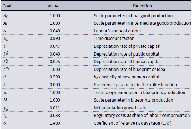
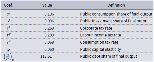
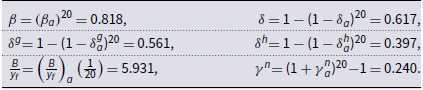
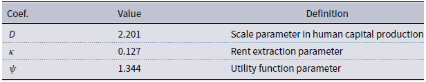
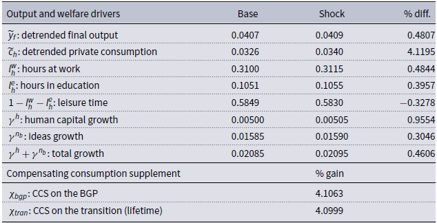


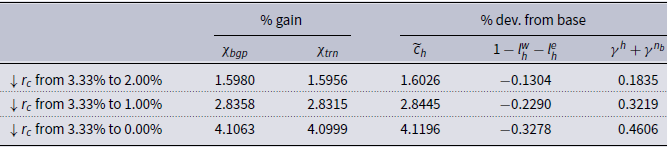
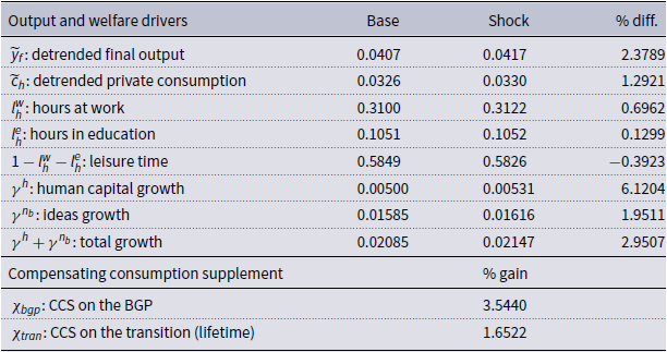


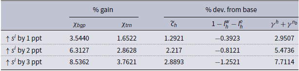
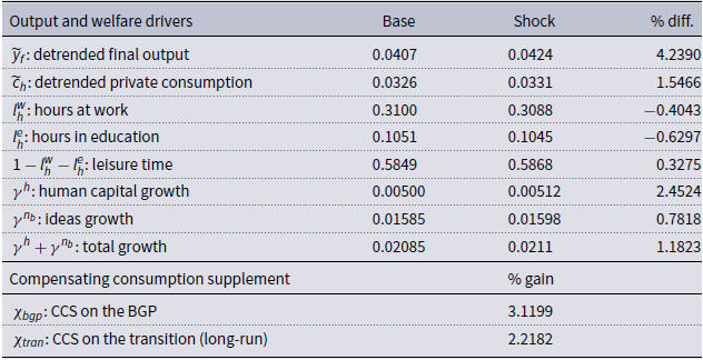

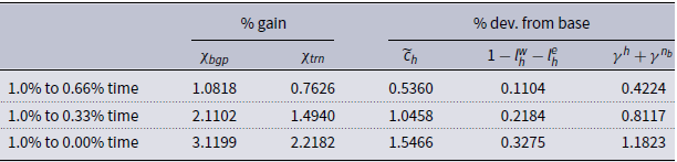


 Open access