
 w
w w
w





1 Introduction
Answer Set Programming (Brewka et al. Reference Brewka, Delgrande, Romero and Schaub2011) (ASP) is a well-established declarative formalism that has been widely adopted for modeling and solving hard combinatorial problems. Over the years, ASP has been successfully applied in a variety of real-world domains, including planning (Son et al. Reference Son, Pontelli, Balduccini and Schaub2023), scheduling (Dodaro et al. Reference Dodaro, Galatà, Maratea and Porro2018; Cardellini et al. Reference Cardellini, Nardi, Dodaro, Galatà, Giardini, Maratea and Porro2021), business process management (Chiariello et al. Reference Chiariello, Fionda, Ielo and Ricca2024; Fionda et al. Reference Fionda, Ielo and Ricca2024), among many others (Eiter et al. Reference Eiter, Fink, Greco and Lembo2008). A substantial body of research has focused on extending ASP modeling and solving capabilities, leading to the proposal of several language extensions (Bogaerts et al. Reference Bogaerts, Janhunen and Tasharrofi2016; Amendola et al. Reference Amendola, Ricca and Truszczynski2019; Fandinno et al. Reference Fandinno, Laferrière, Romero, Schaub and Son2021). Among these, Answer Set Programming with Quantifiers (Amendola et al. Reference Amendola, Ricca and Truszczynski2019) (ASP(Q)) introduces the possibility to quantify over answer sets (Gelfond and Lifschitz Reference Gelfond and Lifschitz1991). This extension enhances the expressive power of ASP, allowing for the natural modeling of problems spanning the entire polynomial hierarchy (PH). ASP(Q) has found interesting applications in several contexts, including outlier detection (Bellusci et al. Reference Bellusci, Mazzotta and Ricca2022), planning (Faber et al. Reference Faber, Morak and Chrpa2022), and related domains (Faber Reference Faber2024), establishing it as a promising framework for solving problems beyond NP. More recently, ASP(Q) has been extended with weak constraints, denoted by ASP $^w$
(Q) (Mazzotta et al. Reference Mazzotta, Ricca and Truszczynski2024), further enhancing its ability to naturally represent hard optimization problems. Weak constraints in ASP
$^w$
(Q) (Mazzotta et al. Reference Mazzotta, Ricca and Truszczynski2024), further enhancing its ability to naturally represent hard optimization problems. Weak constraints in ASP $^w$
(Q) can be applied both locally to enable quantification over optimal answer sets and globally to express preferences among solutions, thus capturing optimization problems throughout the PH. While weak constraints improve the modeling capabilities of ASP(Q), they introduce additional sources of computational complexity, making the design of effective solving techniques challenging (Azzolini et al. Reference Azzolini, Leone, Mazzotta, Ricca, Amin and Arias2026).
$^w$
(Q) can be applied both locally to enable quantification over optimal answer sets and globally to express preferences among solutions, thus capturing optimization problems throughout the PH. While weak constraints improve the modeling capabilities of ASP(Q), they introduce additional sources of computational complexity, making the design of effective solving techniques challenging (Azzolini et al. Reference Azzolini, Leone, Mazzotta, Ricca, Amin and Arias2026).
Within this context, we focus on ASP(Q) programs with two quantifiers and weak constraints, denoted as 2-ASP $^w$
(Q), which are expressive enough to model complex optimization problems up to
$^w$
(Q), which are expressive enough to model complex optimization problems up to $\Delta ^P_3$
. Indeed, the expressive power of 2-ASP
$\Delta ^P_3$
. Indeed, the expressive power of 2-ASP $^w$
(Q) is not yet fully characterized, as existing completeness results are available only for specific language fragments (Mazzotta et al. Reference Mazzotta, Ricca and Truszczynski2024). As a consequence, the development of efficient and complexity-aware implementations for the entire 2-ASP
$^w$
(Q) is not yet fully characterized, as existing completeness results are available only for specific language fragments (Mazzotta et al. Reference Mazzotta, Ricca and Truszczynski2024). As a consequence, the development of efficient and complexity-aware implementations for the entire 2-ASP $^w$
(Q) has so far been left unexplored. To fill this gap, this paper undertakes a complexity analysis of the main reasoning tasks for 2-ASP
$^w$
(Q) has so far been left unexplored. To fill this gap, this paper undertakes a complexity analysis of the main reasoning tasks for 2-ASP $^w$
(Q) programs, namely coherence and brave reasoning, and derives tight completeness results for the general case.
$^w$
(Q) programs, namely coherence and brave reasoning, and derives tight completeness results for the general case.
Moreover, the paper introduces efficient solving techniques for 2-ASP $^w$
(Q). In particular, we propose an efficient evaluation technique based in Counterexample-Guided Abstraction Refinement (CEGAR) (Clarke et al. Reference Clarke, Fehnker, Han, Krogh, Ouaknine, Stursberg and Theobald2003; Janota et al. Reference Janota, Klieber, Marques-Silva and Clarke2016), which serves as the foundation for two algorithms computing optimal quantified answer sets. Although inspired by the lower- and upper-bound improving strategies used in ASP solvers (Alviano et al. Reference Alviano, Dodaro, Marques-Silva and Ricca2020), our lower-bound improving approach departs from existing methods by realizing lower-bound improvement via abstraction refinement instead of unsatisfiable-core extraction, thereby yielding a distinctive and novel technique.
$^w$
(Q). In particular, we propose an efficient evaluation technique based in Counterexample-Guided Abstraction Refinement (CEGAR) (Clarke et al. Reference Clarke, Fehnker, Han, Krogh, Ouaknine, Stursberg and Theobald2003; Janota et al. Reference Janota, Klieber, Marques-Silva and Clarke2016), which serves as the foundation for two algorithms computing optimal quantified answer sets. Although inspired by the lower- and upper-bound improving strategies used in ASP solvers (Alviano et al. Reference Alviano, Dodaro, Marques-Silva and Ricca2020), our lower-bound improving approach departs from existing methods by realizing lower-bound improvement via abstraction refinement instead of unsatisfiable-core extraction, thereby yielding a distinctive and novel technique.
Finally, the proposed techniques have been implemented on top of the CASPER system (Cuteri et al. Reference Cuteri, Mazzotta and Ricca2026). Experimental results demonstrate the effectiveness of our approach across several benchmarks drawn from diverse application domains, confirming both its practical viability and its alignment with the theoretical complexity results.
2 Background
In this section, we provide some preliminaries and notation on ASP and ASP(Q).
2.1 Answer Set Programming
2.1.1 Syntax
A term is a constant (i.e., an integer or a string starting with lowercase letter) or a variable (i.e., a string starting with uppercase letter). An atom is an expression of the form $p(\kern-0.6pt\vec {\kern0.2pt t}\kern1.5pt)$
with
$p(\kern-0.6pt\vec {\kern0.2pt t}\kern1.5pt)$
with $\vec {t}=t_1,\ldots ,t_n$
being a list of terms and
$\vec {t}=t_1,\ldots ,t_n$
being a list of terms and $p$
being a predicate of arity
$p$
being a predicate of arity $n\ge 0$
. An atom
$n\ge 0$
. An atom $p(\kern-0.6pt\vec {\kern0.2pt t}\kern1.5pt)$
is ground if all terms in
$p(\kern-0.6pt\vec {\kern0.2pt t}\kern1.5pt)$
is ground if all terms in $\vec {t}$
are constants. A literal is either an atom
$\vec {t}$
are constants. A literal is either an atom $a$
or its negation
$a$
or its negation ${\scriptstyle \mathtt {\sim }} a$
. The complement of a literal
${\scriptstyle \mathtt {\sim }} a$
. The complement of a literal $l = a$
(resp.
$l = a$
(resp. $l={\scriptstyle \mathtt {\sim }} a$
) is
$l={\scriptstyle \mathtt {\sim }} a$
) is $\overline {l} = {\scriptstyle \mathtt {\sim }} a$
(resp.
$\overline {l} = {\scriptstyle \mathtt {\sim }} a$
(resp. $\overline {l} = a$
). Given a set of literals
$\overline {l} = a$
). Given a set of literals $L$
,
$L$
, $L^+$
(resp.
$L^+$
(resp. $L^-$
) denotes the set of positive (resp. negative) literals appearing in
$L^-$
) denotes the set of positive (resp. negative) literals appearing in $L$
. A rule is an expression of the form
$L$
. A rule is an expression of the form $h \leftarrow l_1, \ldots , l_n$
where
$h \leftarrow l_1, \ldots , l_n$
where $h$
is an atom referred to as head, and
$h$
is an atom referred to as head, and $l_1,\ldots ,l_n$
with
$l_1,\ldots ,l_n$
with $n\ge 0$
is a conjunction of literals referred to as body. A rule with empty body is called fact, while a rule with empty head is called hard constraint. A weak constraint is an expression of the form
$n\ge 0$
is a conjunction of literals referred to as body. A rule with empty body is called fact, while a rule with empty head is called hard constraint. A weak constraint is an expression of the form $\leftarrow ^{\omega } l_1, \ldots , l_n\ [w@l,\vec {t}\,]$
where
$\leftarrow ^{\omega } l_1, \ldots , l_n\ [w@l,\vec {t}\,]$
where $l_1, \ldots , l_n$
is a conjunction of literals referred to as body,
$l_1, \ldots , l_n$
is a conjunction of literals referred to as body, $w$
and
$w$
and $l$
are terms, and
$l$
are terms, and $\vec {t}= t_1, \ldots , t_m$
is a possibly empty list of terms. Given a rule (resp. a weak constraint)
$\vec {t}= t_1, \ldots , t_m$
is a possibly empty list of terms. Given a rule (resp. a weak constraint) $r$
,
$r$
, $H_r$
denotes the set of atoms appearing in the head of
$H_r$
denotes the set of atoms appearing in the head of $r$
while
$r$
while $B_r$
denotes the set of literals appearing in the body of
$B_r$
denotes the set of literals appearing in the body of $r$
. A rule
$r$
. A rule $r$
(resp. a weak constraint) is safe if each variable appears in at least one literal in
$r$
(resp. a weak constraint) is safe if each variable appears in at least one literal in $B_r^+$
. A program
$B_r^+$
. A program $P$
is a set of safe rules and weak constraints. Given a program
$P$
is a set of safe rules and weak constraints. Given a program $P$
,
$P$
, $\mathcal{R}(P)$
, and
$\mathcal{R}(P)$
, and $\mathcal{W}(P)$
denote, respectively, the sets of rules and weak constraints appearing in
$\mathcal{W}(P)$
denote, respectively, the sets of rules and weak constraints appearing in $P$
; while
$P$
; while $\mathcal{H}(P)$
denotes the set of atoms appearing in the head of some rules in
$\mathcal{H}(P)$
denotes the set of atoms appearing in the head of some rules in $P$
. Given an expression
$P$
. Given an expression $\epsilon$
(atom, program, etc.),
$\epsilon$
(atom, program, etc.), $at(\epsilon )$
denotes the set of atoms appearing in
$at(\epsilon )$
denotes the set of atoms appearing in $\epsilon$
.
$\epsilon$
.
2.1.2 Semantics
Given an ASP program $P$
, the Herbrand Universe,
$P$
, the Herbrand Universe, $HU_P$
, of
$HU_P$
, of $P$
is the set of all constants appearing in
$P$
is the set of all constants appearing in $P$
; the Herbrand Base,
$P$
; the Herbrand Base, $B_P$
, is the set of all possible ground atoms that can be obtained from predicates and constants in
$B_P$
, is the set of all possible ground atoms that can be obtained from predicates and constants in $P$
;
$P$
; $ground(P)$
denotes the set of all ground rules that can be obtained from
$ground(P)$
denotes the set of all ground rules that can be obtained from $P$
by proper substitutions of variables in
$P$
by proper substitutions of variables in $P$
with constants in
$P$
with constants in $HU_P$
. An interpretation
$HU_P$
. An interpretation $I \subseteq B_P$
is a set of atoms. A ground literal
$I \subseteq B_P$
is a set of atoms. A ground literal $l=a$
(resp.
$l=a$
(resp. $l={\scriptstyle \mathtt {\sim }} a$
) is true w.r.t.
$l={\scriptstyle \mathtt {\sim }} a$
) is true w.r.t. $I$
if
$I$
if $a \in I$
(resp.
$a \in I$
(resp. $a \notin I$
), false otherwise. A conjunction of literals
$a \notin I$
), false otherwise. A conjunction of literals $conj$
is true w.r.t.
$conj$
is true w.r.t. $I$
if all the literals in
$I$
if all the literals in $conj$
are true w.r.t.
$conj$
are true w.r.t. $I$
, false otherwise. An interpretation
$I$
, false otherwise. An interpretation $I$
is an answer set of
$I$
is an answer set of $P$
iff (
$P$
iff ( $i$
)
$i$
) $I$
is a model of
$I$
is a model of $P$
, namely for each rule
$P$
, namely for each rule $r \in ground(P)$
either
$r \in ground(P)$
either $H_r$
is true w.r.t.
$H_r$
is true w.r.t. $I$
or
$I$
or $B_r$
is false w.r.t.
$B_r$
is false w.r.t. $I$
; and (
$I$
; and ( $ii$
)
$ii$
) $I$
is a minimal model of its GL-reduct (Gelfond and Lifschitz Reference Gelfond and Lifschitz1991). Let
$I$
is a minimal model of its GL-reduct (Gelfond and Lifschitz Reference Gelfond and Lifschitz1991). Let $AS(P)$
be the set of answer set of a program
$AS(P)$
be the set of answer set of a program $P$
, then
$P$
, then $P$
is coherent iff
$P$
is coherent iff $AS(P)\neq \emptyset$
. For a program
$AS(P)\neq \emptyset$
. For a program $P$
and an interpretation
$P$
and an interpretation $I$
, let the set of weak constraint violations be
$I$
, let the set of weak constraint violations be $ws(P,I) = \{(w,l,\kern-1.5pt\vec {\kern1pt t}\kern1.3pt) \mid \ \leftarrow ^{\omega } b_1,\ldots ,b_m\ [w@l,\kern-1.5pt\vec {\kern1pt t}\kern1.9pt] \in ground(P)$
and
$ws(P,I) = \{(w,l,\kern-1.5pt\vec {\kern1pt t}\kern1.3pt) \mid \ \leftarrow ^{\omega } b_1,\ldots ,b_m\ [w@l,\kern-1.5pt\vec {\kern1pt t}\kern1.9pt] \in ground(P)$
and $b_1,\ldots ,b_m$
are true w.r.t.
$b_1,\ldots ,b_m$
are true w.r.t. $I\}$
, then the cost function of
$I\}$
, then the cost function of $P$
is defined as
$P$
is defined as $\mathcal{C}(P,I,k) = \sum _{(w,k,\kern-1.5pt\vec {\kern1pt t}\kern1.3pt) \in ws(P,I)} w$
for every integer
$\mathcal{C}(P,I,k) = \sum _{(w,k,\kern-1.5pt\vec {\kern1pt t}\kern1.3pt) \in ws(P,I)} w$
for every integer $k$
. Let
$k$
. Let $M_1,M_2 \in AS(P)$
then
$M_1,M_2 \in AS(P)$
then $M_1$
is dominated by
$M_1$
is dominated by $M_2$
if there exists an integer
$M_2$
if there exists an integer $l$
such that
$l$
such that $\mathcal{C}(P,M_1,l)\gt \mathcal{C}(P,M_2,l)$
and for each
$\mathcal{C}(P,M_1,l)\gt \mathcal{C}(P,M_2,l)$
and for each $l'\gt l$
,
$l'\gt l$
, $\mathcal{C}(P,M_1,l') = \mathcal{C}(P,M_2,l')$
. Let
$\mathcal{C}(P,M_1,l') = \mathcal{C}(P,M_2,l')$
. Let $M \in AS(P)$
then
$M \in AS(P)$
then $M$
is an optimal answer set iff
$M$
is an optimal answer set iff $M$
is not dominated by any
$M$
is not dominated by any $M' \in AS(P)$
. We denote by
$M' \in AS(P)$
. We denote by $OptAS(P)$
the set of optimal answer set of
$OptAS(P)$
the set of optimal answer set of $P$
.
$P$
.
2.2 ASP with two quantifiers
A 2-ASP $^w$
(Q) program (Mazzotta et al. Reference Mazzotta, Ricca and Truszczynski2024) is an expression of the form
$^w$
(Q) program (Mazzotta et al. Reference Mazzotta, Ricca and Truszczynski2024) is an expression of the form $\Box _1 P_1 \Box _2 P_2: C : C^\omega$
, where
$\Box _1 P_1 \Box _2 P_2: C : C^\omega$
, where $\Box _1,\Box _2$
are quantifiers in
$\Box _1,\Box _2$
are quantifiers in $\{\exists ^{st}, \forall ^{st}\}$
,
$\{\exists ^{st}, \forall ^{st}\}$
, $P_1,P_2$
are ASP programs possibly with weak constraints,
$P_1,P_2$
are ASP programs possibly with weak constraints, $C$
is a stratified program (Ceri et al. Reference Ceri, Gottlob and Tanca1990) with hard constraints, and
$C$
is a stratified program (Ceri et al. Reference Ceri, Gottlob and Tanca1990) with hard constraints, and $C^\omega$
is a set of weak constraints such that
$C^\omega$
is a set of weak constraints such that $B_{C^{\omega }}\subseteq B_{P_1}$
. Weak constraints appearing
$B_{C^{\omega }}\subseteq B_{P_1}$
. Weak constraints appearing $P_1$
and
$P_1$
and $P_2$
are said local; whereas those in
$P_2$
are said local; whereas those in $C^{\omega }$
are said global. A 2-ASP
$C^{\omega }$
are said global. A 2-ASP $^w$
(Q) program
$^w$
(Q) program $\Pi$
is said to be existential if
$\Pi$
is said to be existential if $\Box _1 = \exists ^{st}$
, otherwise it is universal. Moreover,
$\Box _1 = \exists ^{st}$
, otherwise it is universal. Moreover, $\Pi$
is said to be alternating if
$\Pi$
is said to be alternating if $\Box _1\neq \Box _2$
, and plain if it contains no weak constraints. We now define the semantics of 2-ASP
$\Box _1\neq \Box _2$
, and plain if it contains no weak constraints. We now define the semantics of 2-ASP $^w$
(Q) programs. Let
$^w$
(Q) programs. Let $P$
be an ASP program and
$P$
be an ASP program and $M \subseteq B_P$
, then
$M \subseteq B_P$
, then $\mathit{fix_{P}(M)}$
denotes the set of facts and hard constraints of the form
$\mathit{fix_{P}(M)}$
denotes the set of facts and hard constraints of the form $\{a\leftarrow \mid a \in M\} \cup \{\leftarrow a\mid a \in B_P\setminus M\}$
. Then,
$\{a\leftarrow \mid a \in M\} \cup \{\leftarrow a\mid a \in B_P\setminus M\}$
. Then, $M \in AS(P)$
satisfies a program
$M \in AS(P)$
satisfies a program $P'$
if
$P'$
if $P'\cup \mathit{fix_{P}(M)}$
is coherent.
$P'\cup \mathit{fix_{P}(M)}$
is coherent.
At this point the coherence of 2-ASP $^w$
(Q) can be defined as follows:
$^w$
(Q) can be defined as follows:
-
• $\exists ^{st} P: C :C^{\omega }$
is coherent iff there exists
$M \in OptAS(P)$
such that
$M$
satisfies
$C$
.
$\exists ^{st} P: C :C^{\omega }$
is coherent iff there exists
$M \in OptAS(P)$
such that
$M$
satisfies
$C$
. -
•
$\forall ^{st} P: C :C^{\omega }$
is coherent iff for each
$M \in OptAS(P)$
,
$M$
satisfies
$C$
. -
•
$\exists ^{st} P_1 \Box _2 P_2: C :C^{\omega }$
is coherent iff there exists
$M_1 \in OptAS(P_1)$
such that
$\Box _2 P_2 \cup \mathit{fix_{P_1}(M_1)}: C :C^{\omega }$
is coherent. -
•
$\forall ^{st} P_1 \Box _2 P_2: C :C^{\omega }$
is coherent iff for each
$M_1 \in OptAS(P_1)$
,
$\Box _2 P_2 \cup \mathit{fix_{P_1}(M_1)}: C :C^{\omega }$
is coherent.













For an existential 2-ASP $^w$
(Q) program
$^w$
(Q) program $\Pi$
, an optimal answer set
$\Pi$
, an optimal answer set $M_1 \in OptAS(P_1)$
is a quantified answer set of
$M_1 \in OptAS(P_1)$
is a quantified answer set of $\Pi$
if
$\Pi$
if $\Box _2 P_2\cup \mathit{fix_{P_1}(M_1)}:C:C^{\omega }$
is coherent. We denote by
$\Box _2 P_2\cup \mathit{fix_{P_1}(M_1)}:C:C^{\omega }$
is coherent. We denote by $QAS(\Pi )$
the set of quantified answer sets of
$QAS(\Pi )$
the set of quantified answer sets of $\Pi$
. Let
$\Pi$
. Let $\Pi$
be an existential 2-ASP
$\Pi$
be an existential 2-ASP $^w$
(Q) program,
$^w$
(Q) program, $l$
be an integer, and
$l$
be an integer, and $M \in QAS(\Pi )$
, then the cost of
$M \in QAS(\Pi )$
, then the cost of $M$
at level
$M$
at level $l$
is defined as
$l$
is defined as $\mathcal{C}(M,\Pi ,l) = \mathcal{C}(M,P_1\cup C^{\omega },l)$
. Let
$\mathcal{C}(M,\Pi ,l) = \mathcal{C}(M,P_1\cup C^{\omega },l)$
. Let $M_1,M_2 \in QAS(\Pi )$
, then
$M_1,M_2 \in QAS(\Pi )$
, then $M_1$
is dominated by
$M_1$
is dominated by $M_2$
if there exists
$M_2$
if there exists $l$
such that
$l$
such that $\mathcal{C}(M_1,\Pi ,l) \gt \mathcal{C}(M_2,\Pi ,l)$
and for each
$\mathcal{C}(M_1,\Pi ,l) \gt \mathcal{C}(M_2,\Pi ,l)$
and for each $l'\gt l$
,
$l'\gt l$
, $\mathcal{C}(M_1,\Pi ,l') = \mathcal{C}(M_2,\Pi ,l')$
. Thus,
$\mathcal{C}(M_1,\Pi ,l') = \mathcal{C}(M_2,\Pi ,l')$
. Thus, $M$
is an optimal quantified answer set if
$M$
is an optimal quantified answer set if $M$
is not dominated by any
$M$
is not dominated by any $M'\in QAS(\Pi )$
. We denote by
$M'\in QAS(\Pi )$
. We denote by $OptQAS(\Pi )$
the set of optimal quantified answer sets.
$OptQAS(\Pi )$
the set of optimal quantified answer sets.
Example 1. Let $\Pi$
be a 2-ASP
$\Pi$
be a 2-ASP $^w$
(Q) program of the form
$^w$
(Q) program of the form $\exists ^{st} P_1\forall ^{st}P_2:C$
, where
$\exists ^{st} P_1\forall ^{st}P_2:C$
, where $C=\{\leftarrow nb,\ nc\}$
and
$C=\{\leftarrow nb,\ nc\}$
and
 \begin{equation*} P_1 = \left \{\begin{array}{lr} a \leftarrow {\scriptstyle \mathtt {\sim }} na\qquad\qquad & b \leftarrow {\scriptstyle \mathtt {\sim }} nb\\ na \leftarrow {\scriptstyle \mathtt {\sim }} a\qquad\qquad & nb \leftarrow {\scriptstyle \mathtt {\sim }} b\\ \end{array}\right \}\qquad P_2 = \left \{\begin{array}{ll} c \leftarrow {\scriptstyle \mathtt {\sim }} nc\qquad\qquad & \leftarrow ^{\omega } a,\ {\scriptstyle \mathtt {\sim }} c\ [1@1]\\ nc \leftarrow {\scriptstyle \mathtt {\sim }} c\qquad\qquad & \leftarrow ^{\omega } b,\ {\scriptstyle \mathtt {\sim }} nc\ [1@1]\\ \end{array}\right \} \end{equation*}
Let us consider $M_1 = \{na,nb\} \in AS(P_1)$
. In this case,
$M_1 = \{na,nb\} \in AS(P_1)$
. In this case, $\{na,nb,nc\} \in OptAS(P_2\cup \mathit{fix_{P_1}(M_1)})$
violates the constraint
$\{na,nb,nc\} \in OptAS(P_2\cup \mathit{fix_{P_1}(M_1)})$
violates the constraint $\leftarrow nb,nc \in C$
. Thus,
$\leftarrow nb,nc \in C$
. Thus, $M_1\notin QAS(\Pi )$
. Conversely,
$M_1\notin QAS(\Pi )$
. Conversely, $M_1' = \{a,nb\}\in AS(P_1)$
is such that
$M_1' = \{a,nb\}\in AS(P_1)$
is such that $P_2\cup \mathit{fix_{P_1}(M_1')}$
admits only one optimal answer set
$P_2\cup \mathit{fix_{P_1}(M_1')}$
admits only one optimal answer set $M_2 = \{a,nb,c\}$
which satisfies the constraint in
$M_2 = \{a,nb,c\}$
which satisfies the constraint in $C$
and so
$C$
and so $M_1\in QAS(\Pi )$
. If we remove weak constraints from
$M_1\in QAS(\Pi )$
. If we remove weak constraints from $P_2$
, then
$P_2$
, then $AS(P_2\cup \mathit{fix_{P_1}(M_1)}) = \{M_2, M_2'\}$
where
$AS(P_2\cup \mathit{fix_{P_1}(M_1)}) = \{M_2, M_2'\}$
where $M_2' = \{a,nb,nc\}$
. Here,
$M_2' = \{a,nb,nc\}$
. Here, $M_2'$
violates the constraint in
$M_2'$
violates the constraint in $C$
and so
$C$
and so $M_1$
is not a quantified answer set anymore.
$M_1$
is not a quantified answer set anymore.
3 Complexity results for 2-ASP
$^w$
(Q)

In this section, we study the main computational tasks for 2-ASP $^w$
(Q): Coherence and Brave reasoning. For 2-ASP
$^w$
(Q): Coherence and Brave reasoning. For 2-ASP $^w$
(Q) programs, the coherence problem checks whether a program is coherent, while brave reasoning verifies whether an atom occurs in an optimal quantified answer set. Unlike standard ASP, local weak constraints in ASP
$^w$
(Q) programs, the coherence problem checks whether a program is coherent, while brave reasoning verifies whether an atom occurs in an optimal quantified answer set. Unlike standard ASP, local weak constraints in ASP $^w$
(Q) programs introduce an additional source of computational complexity, as observed by Mazzotta et al. (Reference Mazzotta, Ricca and Truszczynski2024). Even though complexity results for these tasks have been established for specific subclasses of ASP
$^w$
(Q) programs introduce an additional source of computational complexity, as observed by Mazzotta et al. (Reference Mazzotta, Ricca and Truszczynski2024). Even though complexity results for these tasks have been established for specific subclasses of ASP $^w$
(Q), a complete characterization is still missing.
$^w$
(Q), a complete characterization is still missing.
In particular, it was shown that verifying the coherence for 2-ASP $^w$
(Q) programs (
$^w$
(Q) programs ( $i$
) is in
$i$
) is in $\Sigma _3^P$
for existential programs and in
$\Sigma _3^P$
for existential programs and in $\Pi _3^P$
for universal programs, and (
$\Pi _3^P$
for universal programs, and ( $ii$
) is hard for
$ii$
) is hard for $\Sigma _2^P$
and
$\Sigma _2^P$
and $\Pi _2^P$
, respectively. Starting from these results, we prove that the coherence problem for 2-ASP
$\Pi _2^P$
, respectively. Starting from these results, we prove that the coherence problem for 2-ASP $^w$
(Q) is complete for the second level of the PH, namely
$^w$
(Q) is complete for the second level of the PH, namely $\Sigma _2^P$
for existential programs and
$\Sigma _2^P$
for existential programs and $\Pi _2^P$
for universal programs (full proofs in the online appendix).
$\Pi _2^P$
for universal programs (full proofs in the online appendix).
Theorem 1 (Membership). The coherence problem for 2-ASP $^w$
(Q) programs of the form
$^w$
(Q) programs of the form $\Box _1 P_1\Box _2 P_2:C$
is in:
$\Box _1 P_1\Box _2 P_2:C$
is in: $\Sigma _2^P$
if
$\Sigma _2^P$
if $\Box _1 = \exists ^{st}$
;
$\Box _1 = \exists ^{st}$
; $\Pi _2^P$
otherwise, no matter whether
$\Pi _2^P$
otherwise, no matter whether $\Box _2 = \exists ^{st}$
or
$\Box _2 = \exists ^{st}$
or $\Box _2 = \forall ^{st}$
Proof (Sketch) To prove our thesis we need to distinguish three different scenarios.
Uniform quantifiers $\Box _1 = \Box _2$
. By applying the transformation (Algorithm 1) by Mazzotta et al. (Reference Mazzotta, Ricca and Truszczynski2024), it is possible to obtain a plain 2-ASP(Q) program
$\Box _1 = \Box _2$
. By applying the transformation (Algorithm 1) by Mazzotta et al. (Reference Mazzotta, Ricca and Truszczynski2024), it is possible to obtain a plain 2-ASP(Q) program $\Pi '$
such that
$\Pi '$
such that $\Pi '$
is coherent if and only if
$\Pi '$
is coherent if and only if $\Pi$
is coherent. From the result of Amendola et al. (Reference Amendola, Ricca and Truszczynski2019), verifying the coherence of
$\Pi$
is coherent. From the result of Amendola et al. (Reference Amendola, Ricca and Truszczynski2019), verifying the coherence of $\Pi '$
is
$\Pi '$
is $\Sigma _2^P$
-complete if
$\Sigma _2^P$
-complete if $\Box _1 = \exists ^{st}$
; otherwise is in
$\Box _1 = \exists ^{st}$
; otherwise is in $\Pi _2^P$
-complete. Thus the thesis holds for uniform quantifiers.
$\Pi _2^P$
-complete. Thus the thesis holds for uniform quantifiers.
Case $\Box _1 = \exists ^{st}$
and
$\Box _1 = \exists ^{st}$
and $\Box _2 = \forall ^{st}$
. In this case, it is possible to translate
$\Box _2 = \forall ^{st}$
. In this case, it is possible to translate $\Pi$
into an existential 2-ASP
$\Pi$
into an existential 2-ASP $^w$
(Q) program
$^w$
(Q) program $\Pi '$
where weak constraints appear only in the first subprogram. Since verifying the coherence of
$\Pi '$
where weak constraints appear only in the first subprogram. Since verifying the coherence of $\Pi '$
is
$\Pi '$
is $\Sigma _2^P$
-complete (Corollary 3.1 by Mazzotta et al. Reference Mazzotta, Ricca and Truszczynski2024), then the thesis holds also in this case.
$\Sigma _2^P$
-complete (Corollary 3.1 by Mazzotta et al. Reference Mazzotta, Ricca and Truszczynski2024), then the thesis holds also in this case.
More precisely, the 2-ASP $^w$
(Q) program
$^w$
(Q) program $\Pi '$
can be obtained by copying the rules of the program
$\Pi '$
can be obtained by copying the rules of the program $P_2$
in
$P_2$
in $P_1$
and then adding rules in the program
$P_1$
and then adding rules in the program $C$
for verifying the optimality of an answer sets of
$C$
for verifying the optimality of an answer sets of $P_2$
. As a result, we obtain
$P_2$
. As a result, we obtain $\Pi '$
of the form
$\Pi '$
of the form $\exists P_1' \forall P_2': C'$
where:
$\exists P_1' \forall P_2': C'$
where:
-
• optimal answer sets
$M$
of
$P_1'$
are of the form
$M_1 \cup M_2^c$
where
$M_1$
is an optimal answer set of
$P_1$
and
$M$
corresponds to an answer set of
$P_2\cup \mathit{fix_{P_1}(M_1)}$
; -
• answer sets
$N$
of
$P_2'\cup \mathit{fix_{P_1'}(M)}$
are of the form
$M_1 \cup M_2^c \cup M_2$
where
$M_1\cup M_2$
is an answer set of
$P_2\cup \mathit{fix_{P_1}(M_1)}$
; -
• an answer set
$N$
of
$P_2'\cup \mathit{fix_{P_1'}(M)}$
satisfies
$C'$
if and only if
$M_1 \cup M_2^c$
is not dominated by
$M_1 \cup M_2$
and one of the following holds:










-
– there exists
$l$
such that the cost of
$M_1 \cup M_2$
is different from the cost of
$M_1\cup M_2^c$
; -
– the cost of
$M_1\cup M_2$
is equal to the cost of
$M_1\cup M_2^c$
for each level and
$M_1 \cup M_2$
satisfies
$C$
.


Let $M = M_1 \cup M_2^c$
be an optimal answer set of
$M = M_1 \cup M_2^c$
be an optimal answer set of $P_1'$
. If
$P_1'$
. If $M$
is not an optimal answer set of
$M$
is not an optimal answer set of $P_2\cup \mathit{fix_{P_1}(M_1)}$
, then
$P_2\cup \mathit{fix_{P_1}(M_1)}$
, then $M$
cannot be a quantified answer set as there exists
$M$
cannot be a quantified answer set as there exists $N = M_1 \cup M_2^c \cup M_2$
in the answer sets of
$N = M_1 \cup M_2^c \cup M_2$
in the answer sets of $P_2'\cup \mathit{fix_{P}(M)}$
, where
$P_2'\cup \mathit{fix_{P}(M)}$
, where $M_1 \cup M_2$
is an optimal answer set of
$M_1 \cup M_2$
is an optimal answer set of $P_2\cup \mathit{fix_{P_1}(M_1)}$
and
$P_2\cup \mathit{fix_{P_1}(M_1)}$
and $N$
violates
$N$
violates $C'$
since
$C'$
since $M_1\cup M_2^c$
is dominated by
$M_1\cup M_2^c$
is dominated by $M_1 \cup M_2$
. On the other hand, since
$M_1 \cup M_2$
. On the other hand, since $M$
is an optimal answer set of
$M$
is an optimal answer set of $P_2\cup \mathit{fix_{P_1}(M_1)}$
, then for each
$P_2\cup \mathit{fix_{P_1}(M_1)}$
, then for each $N = M_1 \cup M_2^c \cup M_2$
in the answer sets of
$N = M_1 \cup M_2^c \cup M_2$
in the answer sets of $P_2'\cup \mathit{fix_{P_1'}(M)}$
,
$P_2'\cup \mathit{fix_{P_1'}(M)}$
, $M_1\cup M_2^c$
is not dominated by
$M_1\cup M_2^c$
is not dominated by $M_1\cup M_2$
(i.e., Condition 1 is always satisfied). Thus, let
$M_1\cup M_2$
(i.e., Condition 1 is always satisfied). Thus, let $N = M_1\cup M_2^c \cup M_2$
be an answer set of
$N = M_1\cup M_2^c \cup M_2$
be an answer set of $P_2\cup \mathit{fix_{P_1'}(M)}$
, then
$P_2\cup \mathit{fix_{P_1'}(M)}$
, then $N$
satisfies
$N$
satisfies $C'$
if and only if one between Conditions 1 and 2 holds. Here we can observe that Condition 1 holds if and only if
$C'$
if and only if one between Conditions 1 and 2 holds. Here we can observe that Condition 1 holds if and only if $M_1\cup M_2$
is not an optimal answer set of
$M_1\cup M_2$
is not an optimal answer set of $P_2\cup \mathit{fix_{P_1}(M_1)}$
; whereas Condition 2 holds if and only if
$P_2\cup \mathit{fix_{P_1}(M_1)}$
; whereas Condition 2 holds if and only if $M_1\cup M_2$
is an optimal answer set of
$M_1\cup M_2$
is an optimal answer set of $P_2\cup \mathit{fix_{P_1}(M_1)}$
and
$P_2\cup \mathit{fix_{P_1}(M_1)}$
and $M_1\cup M_2$
satisfies
$M_1\cup M_2$
satisfies $C$
. Thus,
$C$
. Thus, $M$
is a quantified answer set of
$M$
is a quantified answer set of $\Pi '$
if and only if each optimal answer set
$\Pi '$
if and only if each optimal answer set $M_1\cup M_2$
of
$M_1\cup M_2$
of $P_2\cup \mathit{fix_{P_1}(M_1)}$
satisfies
$P_2\cup \mathit{fix_{P_1}(M_1)}$
satisfies $C$
. Hence,
$C$
. Hence, $M$
is a quantified answer set of
$M$
is a quantified answer set of $\Pi '$
if and only if
$\Pi '$
if and only if $M_1$
is a quantified answer set of
$M_1$
is a quantified answer set of $\Pi$
. Finally, we can conclude that
$\Pi$
. Finally, we can conclude that $\Pi$
is coherent iff
$\Pi$
is coherent iff $\Pi '$
is coherent.
$\Pi '$
is coherent.
Case $\Box _1 = \forall ^{st}$
and
$\Box _1 = \forall ^{st}$
and $\Box _2 = \exists ^{st}$
. By following the same working principle as before, it is possible to encode
$\Box _2 = \exists ^{st}$
. By following the same working principle as before, it is possible to encode $\Pi$
into a 2-ASP
$\Pi$
into a 2-ASP $^w$
(Q) program
$^w$
(Q) program $\Pi '$
which preserves the coherence of
$\Pi '$
which preserves the coherence of $\Pi$
and in which weak constraints appear only in the first subprogram. In this case, verifying the coherence of
$\Pi$
and in which weak constraints appear only in the first subprogram. In this case, verifying the coherence of $\Pi '$
is
$\Pi '$
is $\Pi _2^P$
-complete (Corollary 3.1 by Mazzotta et al. Reference Mazzotta, Ricca and Truszczynski2024), then the thesis holds also in this last case. In this case, the 2-ASP
$\Pi _2^P$
-complete (Corollary 3.1 by Mazzotta et al. Reference Mazzotta, Ricca and Truszczynski2024), then the thesis holds also in this last case. In this case, the 2-ASP $^w$
(Q) program
$^w$
(Q) program $\Pi '$
is of the form
$\Pi '$
is of the form $\forall P_1' \exists P_2': C'$
where:
$\forall P_1' \exists P_2': C'$
where:
-
• optimal answer sets
$M$
of
$P_1'$
are of the form
$M_1 \cup M_2^c$
where
$M_1$
is an answer set of
$P_1$
and
$M$
is an answer set of
$P_2\cup \mathit{fix_{P_1}(M_1)}$
; -
• answer sets
$N$
of
$P_2'\cup \mathit{fix_{P_1'}(M)}$
are of the form
$M_1 \cup M_2^c \cup M_2$
where
$M_1\cup M_2$
is an answer set of
$P_2\cup \mathit{fix_{P_1}(M_1)}$
; -
• an answer set
$N$
of
$P_2'\cup \mathit{fix_{P_1'}(M)}$
satisfies
$C'$
if and only if one of the following holds:










-
–
$M_1 \cup M_2^c$
is dominated by
$M_1 \cup M_2$
; -
– the cost of
$M_1\cup M_2$
is equal to the cost of
$M_1\cup M_2^c$
for each level and
$M_1 \cup M_2$
satisfies
$C$
.


According to the ASP $^w$
(Q) semantics,
$^w$
(Q) semantics, $\Pi '$
is incoherent if and only if there exists an optimal answer set
$\Pi '$
is incoherent if and only if there exists an optimal answer set $M_1$
of
$M_1$
of $P_1'$
such that for every answer set
$P_1'$
such that for every answer set $N$
of
$N$
of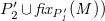 $P_2'\cup \mathit{fix_{P_1'}(M)})$
,
$P_2'\cup \mathit{fix_{P_1'}(M)})$
, $N$
does not satisfy
$N$
does not satisfy $C'$
. Let
$C'$
. Let $M = M_1 \cup M_2^c$
be an optimal answer set of
$M = M_1 \cup M_2^c$
be an optimal answer set of $P_1'$
, with
$P_1'$
, with $M_1\in OptAS(P_1)$
and
$M_1\in OptAS(P_1)$
and $M \in AS(P_2\cup \mathit{fix_{P_1}(M_1)})$
.
$M \in AS(P_2\cup \mathit{fix_{P_1}(M_1)})$
.
If $M_1 \cup M_2^c$
is not an optimal answer set of
$M_1 \cup M_2^c$
is not an optimal answer set of $P_2\cup \mathit{fix_{P_1}(M_1)}$
, then there exists
$P_2\cup \mathit{fix_{P_1}(M_1)}$
, then there exists $M_1 \cup M_2 \in OptAS(P_2\cup \mathit{fix_{P_1}(M_1)})$
such that
$M_1 \cup M_2 \in OptAS(P_2\cup \mathit{fix_{P_1}(M_1)})$
such that $M_1 \cup M_2^c$
is dominated by
$M_1 \cup M_2^c$
is dominated by $M_1 \cup M_2$
. Consequently,
$M_1 \cup M_2$
. Consequently, $N = M_1 \cup M_2^c \cup M_2 \in AS(P_2'\cup \mathit{fix_{P}(M)})$
is such that Condition 1 is satisfied, and thus
$N = M_1 \cup M_2^c \cup M_2 \in AS(P_2'\cup \mathit{fix_{P}(M)})$
is such that Condition 1 is satisfied, and thus $M$
cannot witness the incoherence of
$M$
cannot witness the incoherence of $\Pi '$
.
$\Pi '$
.
Otherwise, $M_1 \cup M_2^c$
is optimal for
$M_1 \cup M_2^c$
is optimal for $P_2\cup \mathit{fix_{P_1}(M_1)}$
. In this case, for every
$P_2\cup \mathit{fix_{P_1}(M_1)}$
. In this case, for every $N = M_1 \cup M_2^c \cup M_2 \in AS(P_2'\cup \mathit{fix_{P_1'}(M)})$
,
$N = M_1 \cup M_2^c \cup M_2 \in AS(P_2'\cup \mathit{fix_{P_1'}(M)})$
, $N$
satisfies
$N$
satisfies $C'$
if and only if Condition 2 holds, that is, if and only if
$C'$
if and only if Condition 2 holds, that is, if and only if $M_1 \cup M_2$
has the same cost of
$M_1 \cup M_2$
has the same cost of $M_1\cup M_2^c$
(i.e.,
$M_1\cup M_2^c$
(i.e., $M_1\cup M_2\in OptAS(P_2\cup \mathit{fix_{P_1}(M_1)})$
) and
$M_1\cup M_2\in OptAS(P_2\cup \mathit{fix_{P_1}(M_1)})$
) and $M_1 \cup M_2$
satisfies
$M_1 \cup M_2$
satisfies $C$
.
$C$
.
Therefore, $\Pi '$
is incoherent if and only if there exists
$\Pi '$
is incoherent if and only if there exists $M_1 \in AS(P_1)$
such that no
$M_1 \in AS(P_1)$
such that no $M_1 \cup M_2 \in OptAS(P_2\cup \mathit{fix_{P_1}(M_1)})$
satisfies
$M_1 \cup M_2 \in OptAS(P_2\cup \mathit{fix_{P_1}(M_1)})$
satisfies $C$
, which is exactly the condition for
$C$
, which is exactly the condition for $\Pi$
to be incoherent. Hence,
$\Pi$
to be incoherent. Hence, $\Pi '$
preserves the coherence of
$\Pi '$
preserves the coherence of $\Pi$
.
$\Pi$
.
Note that, the presence of weak constraints in both quantified programs do not allow for a simple quantifier elimination, and the existing translation proposed by Mazzotta et al. (Reference Mazzotta, Ricca and Truszczynski2024) requires the introduction of an additional quantifier, resulting in a non necessary jump in complexity to the third level of the PH in case $\Box _1 \neq \Box _2$
.
$\Box _1 \neq \Box _2$
.
Theorem 2 (Hardness). The coherence problem for 2-ASP $^w$
(Q) programs of the form
$^w$
(Q) programs of the form $\Box _1 P_1\Box _2 P_2:C$
is hard for:
$\Box _1 P_1\Box _2 P_2:C$
is hard for: $\Sigma _2^P$
if
$\Sigma _2^P$
if $\Box _1 = \exists ^{st}$
;
$\Box _1 = \exists ^{st}$
; $\Pi _2^P$
otherwise, no matter whether
$\Pi _2^P$
otherwise, no matter whether $\Box _2 = \exists ^{st}$
or
$\Box _2 = \exists ^{st}$
or $\Box _2 = \forall ^{st}$
.
$\Box _2 = \forall ^{st}$
.
Proof (Sketch). Let us consider the different combination of quantifiers separately.
(Case $\Box _1 = \Box _2 = \exists ^{st}$
). From Theorem 4 by Mazzotta et al. (Reference Mazzotta, Ricca and Truszczynski2024), deciding the coherence of
$\Box _1 = \Box _2 = \exists ^{st}$
). From Theorem 4 by Mazzotta et al. (Reference Mazzotta, Ricca and Truszczynski2024), deciding the coherence of $\Pi$
is
$\Pi$
is $\Sigma _2^P$
-complete if
$\Sigma _2^P$
-complete if $\mathcal{W}(P_1) = \emptyset$
. Thus, the thesis holds since this is a particular case.
$\mathcal{W}(P_1) = \emptyset$
. Thus, the thesis holds since this is a particular case.
(Case $\Box _1 = \Box _2 = \forall ^{st}$
). Let
$\Box _1 = \Box _2 = \forall ^{st}$
). Let $\Phi = \forall X\exists Y \phi$
be a
$\Phi = \forall X\exists Y \phi$
be a $2$
-QBF, where
$2$
-QBF, where $X$
and
$X$
and $Y$
are disjoint set of variables and
$Y$
are disjoint set of variables and $\phi$
is a boolean formula in 3-CNF. Verifying that
$\phi$
is a boolean formula in 3-CNF. Verifying that $\Phi$
is true is a
$\Phi$
is true is a $\Pi _2^P$
-complete problem (Schaefer and Umans Reference Schaefer and Umans2002). We encode in polynomial time any
$\Pi _2^P$
-complete problem (Schaefer and Umans Reference Schaefer and Umans2002). We encode in polynomial time any $\Phi$
in a 2-ASP
$\Phi$
in a 2-ASP $^w$
(Q) program of the form
$^w$
(Q) program of the form $\forall ^{st} P_1 \forall ^{st} P_2:C$
, as detailed in the online appendix.
$\forall ^{st} P_1 \forall ^{st} P_2:C$
, as detailed in the online appendix.
(Case $\Box _1 \neq \Box _2$
). Deciding the coherence of plain alternating 2-ASP(Q) programs
$\Box _1 \neq \Box _2$
). Deciding the coherence of plain alternating 2-ASP(Q) programs $\Sigma _2^P$
-complete if
$\Sigma _2^P$
-complete if $\Box _1 = \exists ^{st}$
; otherwise it is
$\Box _1 = \exists ^{st}$
; otherwise it is $\Pi _2^P$
-complete (Amendola et al. Reference Amendola, Ricca and Truszczynski2019). Since this is a particular case of 2-ASP
$\Pi _2^P$
-complete (Amendola et al. Reference Amendola, Ricca and Truszczynski2019). Since this is a particular case of 2-ASP $^w$
(Q) (i.e.,
$^w$
(Q) (i.e., $\mathcal{W}(P_1) = \mathcal{W}(P_2) = \emptyset$
), then the thesis follows.
$\mathcal{W}(P_1) = \mathcal{W}(P_2) = \emptyset$
), then the thesis follows.
Theorem 3 (Completeness). The coherence problem for 2-ASP $^w$
(Q) programs of the form
$^w$
(Q) programs of the form $\Box _1 P_1\Box _2 P_2:C$
is:
$\Box _1 P_1\Box _2 P_2:C$
is: $\Sigma _2^P$
-complete if
$\Sigma _2^P$
-complete if $\Box _1 = \exists ^{st}$
;
$\Box _1 = \exists ^{st}$
; $\Pi _2^P$
-complete otherwise, no matter whether
$\Pi _2^P$
-complete otherwise, no matter whether $\Box _2 = \exists ^{st}$
or
$\Box _2 = \exists ^{st}$
or $\Box _2 = \forall ^{st}$
.
$\Box _2 = \forall ^{st}$
.
From Theorem3, we derive complete results for the brave reasoning task in 2-ASP $^w$
(Q), which asks whether an atom
$^w$
(Q), which asks whether an atom $a$
is true in some optimal quantified answer set.
$a$
is true in some optimal quantified answer set.
Theorem 4. Let $\Pi$
be an existential 2-ASP
$\Pi$
be an existential 2-ASP $^w$
(Q) program of the form
$^w$
(Q) program of the form $\Box _1 P_1\Box _2 P_2:C:C^{\omega }$
and
$\Box _1 P_1\Box _2 P_2:C:C^{\omega }$
and $a$
be a ground atom, then verifying whether
$a$
be a ground atom, then verifying whether $a \in M$
, with
$a \in M$
, with $M \in OptQAS(\Pi )$
, is
$M \in OptQAS(\Pi )$
, is $\Delta _{3}^P$
-complete no matter whether
$\Delta _{3}^P$
-complete no matter whether $\Box _2 = \exists ^{st}$
or
$\Box _2 = \exists ^{st}$
or $\Box _2 = \forall ^{st}$
.
$\Box _2 = \forall ^{st}$
.
These results strengthen those of Mazzotta et al. (Reference Mazzotta, Ricca and Truszczynski2024), as they establish completeness for all combinations of quantifiers, rather than for alternating programs only.
4 Solving 2-ASP
$^w$
(Q) via CEGAR

CEGAR (Clarke et al. Reference Clarke, Fehnker, Han, Krogh, Ouaknine, Stursberg and Theobald2003) is an iterative technique that starts from a simplified system representation (abstraction) and progressively refines it using counterexamples, until a solution is found or non-existence is proven. CEGAR-based techniques were successfully applied to QBF-satisfiability (Janota et al. Reference Janota, Klieber, Marques-Silva and Clarke2016) and 2-ASP(Q) solving (Cuteri et al. Reference Cuteri, Mazzotta and Ricca2026). Building on these ideas, we propose a CEGAR-based approach for the evaluation of 2-ASP $^w$
(Q) programs. In the following we give a game-theoretic characterization of the semantics of 2-ASP
$^w$
(Q) programs. In the following we give a game-theoretic characterization of the semantics of 2-ASP $^w$
(Q) and then we focus on the two stages of CEGAR: abstraction refinement and counterexample search.
$^w$
(Q) and then we focus on the two stages of CEGAR: abstraction refinement and counterexample search.
4.1 The 2-ASP
$^w$
(Q) game

Let $\Box \in \{\exists ^{st},\forall ^{st}\}$
be a quantifier, then the opponent of
$\Box \in \{\exists ^{st},\forall ^{st}\}$
be a quantifier, then the opponent of $\Box$
is
$\Box$
is $\overline {\Box } = \forall ^{st}$
if
$\overline {\Box } = \forall ^{st}$
if $\Box = \exists ^{st}$
; otherwise
$\Box = \exists ^{st}$
; otherwise $\overline {\Box } = \exists ^{st}$
. Thus, for any alternating 2-ASP
$\overline {\Box } = \exists ^{st}$
. Thus, for any alternating 2-ASP $^w$
(Q) program
$^w$
(Q) program $\Box _2$
is the opponent of
$\Box _2$
is the opponent of $\Box _1$
, that is,
$\Box _1$
, that is, $\Box _2 = \overline {\Box _1}$
. In what follows, w.l.o.g., we consider 2-ASP
$\Box _2 = \overline {\Box _1}$
. In what follows, w.l.o.g., we consider 2-ASP $^w$
(Q) programs of the form:
$^w$
(Q) programs of the form:
 \begin{equation} \Box P_1\overline {\Box } P_2:C:C^{\omega } \end{equation}
Let $\Pi$
be a 2-ASP
$\Pi$
be a 2-ASP $^w$
(Q) program of the form (1), then a move for
$^w$
(Q) program of the form (1), then a move for $\Box$
is an answer set
$\Box$
is an answer set $M_1 \in OptAS(P_1)$
. Given a move
$M_1 \in OptAS(P_1)$
. Given a move $M_1$
for
$M_1$
for $\Box$
, for each
$\Box$
, for each $M_2 \in OptAS(P_2 \cup \mathit{fix_{P_1}(M_1)})$
,
$M_2 \in OptAS(P_2 \cup \mathit{fix_{P_1}(M_1)})$
, $M_2|_{\mathcal{H}(P_2)}$
is a candidate countermove to
$M_2|_{\mathcal{H}(P_2)}$
is a candidate countermove to $M_1$
for
$M_1$
for $\overline {\Box }$
. Let
$\overline {\Box }$
. Let $M_2 \in OptAS(P_2\cup \mathit{fix_{P_1}(M_1)})$
be a candidate countermove then
$M_2 \in OptAS(P_2\cup \mathit{fix_{P_1}(M_1)})$
be a candidate countermove then $M_2|_{\mathcal{H}(P_2)}$
is effectively a countermove to
$M_2|_{\mathcal{H}(P_2)}$
is effectively a countermove to $M_1$
for
$M_1$
for $\overline {\Box }$
if: (
$\overline {\Box }$
if: ( $i$
)
$i$
) $\Box =\exists ^{st}$
and
$\Box =\exists ^{st}$
and $M_2$
does not satisfies
$M_2$
does not satisfies $C$
; or (
$C$
; or ( $ii$
)
$ii$
) $\Box =\forall ^{st}$
and
$\Box =\forall ^{st}$
and $M_2$
satisfies
$M_2$
satisfies $C$
. A winning move for
$C$
. A winning move for $\Box$
is a move
$\Box$
is a move $M_1$
such that no countermove to
$M_1$
such that no countermove to $M_1$
for
$M_1$
for $\overline {\Box }$
exists. Thus,
$\overline {\Box }$
exists. Thus, $\Box = \exists ^{st}$
wins if there exists
$\Box = \exists ^{st}$
wins if there exists $M_1 \in OptAS(P_1)$
such that no countermove to
$M_1 \in OptAS(P_1)$
such that no countermove to $M_1$
for
$M_1$
for $\overline {\Box }$
exists.
$\overline {\Box }$
exists.
Proposition 1. Let $\Pi$
be a 2-ASP
$\Pi$
be a 2-ASP $^w$
(Q) of the form (1), there exists a winning move for
$^w$
(Q) of the form (1), there exists a winning move for $\Box$
if and only if (
$\Box$
if and only if ( $i$
)
$i$
) $\Box =\exists ^{st}$
and
$\Box =\exists ^{st}$
and $\Pi$
is coherent, or (
$\Pi$
is coherent, or ( $ii$
)
$ii$
) $\Box = \forall ^{st}$
and
$\Box = \forall ^{st}$
and $\Pi$
is incoherent.
$\Pi$
is incoherent.
Intuitively, the notion of winning moves closely corresponds to the definition of coherence of 2-ASP $^w$
(Q) programs. Let
$^w$
(Q) programs. Let $\Pi$
be a 2-ASP
$\Pi$
be a 2-ASP $^w$
(Q) program of the form (1), and let
$^w$
(Q) program of the form (1), and let $M_1$
be a winning move for
$M_1$
be a winning move for $\Box$
. If
$\Box$
. If $\Box = \exists ^{st}$
, then there is no
$\Box = \exists ^{st}$
, then there is no $M_2 \in OptAS(P_2 \cup \mathit{fix_{P_1}(M_1)})$
such that
$M_2 \in OptAS(P_2 \cup \mathit{fix_{P_1}(M_1)})$
such that $M_2$
violates
$M_2$
violates $C$
. This implies that
$C$
. This implies that $\forall ^{st} P_2 \cup \mathit{fix_{P_1}(M_1)} : C$
is coherent, and hence
$\forall ^{st} P_2 \cup \mathit{fix_{P_1}(M_1)} : C$
is coherent, and hence $\Pi$
is coherent. Conversely, if
$\Pi$
is coherent. Conversely, if $\Box = \forall ^{st}$
, then there is no
$\Box = \forall ^{st}$
, then there is no $M_2 \in OptAS(P_2 \cup \mathit{fix_{P_1}(M_1)})$
such that
$M_2 \in OptAS(P_2 \cup \mathit{fix_{P_1}(M_1)})$
such that $M_2$
satisfies
$M_2$
satisfies $C$
. Therefore,
$C$
. Therefore, $\exists ^{st} P_2 \cup \mathit{fix_{P_1}(M_1)} : C$
is incoherent, and thus
$\exists ^{st} P_2 \cup \mathit{fix_{P_1}(M_1)} : C$
is incoherent, and thus $\Pi$
is incoherent.
$\Pi$
is incoherent.
4.2 Counterexample search in 2-ASP
$^w$
(Q)

Given a 2-ASP $^w$
(Q) program
$^w$
(Q) program $\Pi$
of the form (1), from Proposition1, the coherence of
$\Pi$
of the form (1), from Proposition1, the coherence of $\Pi$
can be decided by searching for a winning move for
$\Pi$
can be decided by searching for a winning move for $\Box$
. Thus, the program
$\Box$
. Thus, the program $P_1$
, whose optimal answer sets coincide with the possible moves of
$P_1$
, whose optimal answer sets coincide with the possible moves of $\Box$
, is a natural abstraction for
$\Box$
, is a natural abstraction for $\Pi$
. Hence, given
$\Pi$
. Hence, given $M_1\in OptAS(P_1)$
, the counterexample search aims at contradicting
$M_1\in OptAS(P_1)$
, the counterexample search aims at contradicting $M_1$
, which means finding a countermove to
$M_1$
, which means finding a countermove to $M_1$
for
$M_1$
for $\overline {\Box }$
. To this end, we define the countermove program whose optimal answer sets correspond to countermoves to
$\overline {\Box }$
. To this end, we define the countermove program whose optimal answer sets correspond to countermoves to $M_1$
for
$M_1$
for $\overline {\Box }$
.
$\overline {\Box }$
.
We recall that countermoves correspond to optimal answer sets of $P_2\cup \mathit{fix_{P_1}(M_1)}$
that either satisfy or not the program
$P_2\cup \mathit{fix_{P_1}(M_1)}$
that either satisfy or not the program $C$
according to
$C$
according to $\overline {\Box }$
. Since
$\overline {\Box }$
. Since $C$
is stratified with hard constraints, it admits one answer set (Dantsin et al. Reference Dantsin, Eiter, Gottlob and Voronkov2001) iff hard constraints are satisfied. Thus, the following transformation can be used to capture the incoherence of
$C$
is stratified with hard constraints, it admits one answer set (Dantsin et al. Reference Dantsin, Eiter, Gottlob and Voronkov2001) iff hard constraints are satisfied. Thus, the following transformation can be used to capture the incoherence of $C$
.
$C$
.
Definition 1 (Complement of stratified program). Let $P$
be a stratified ASP program with hard constraints, then the complement of
$P$
be a stratified ASP program with hard constraints, then the complement of $P$
, denoted by
$P$
, denoted by $\neg P$
, is obtained from
$\neg P$
, is obtained from $P$
by (
$P$
by ( $i$
) transforming hard constraints
$i$
) transforming hard constraints $\leftarrow l_1,\ldots ,l_n$
into rules of the form
$\leftarrow l_1,\ldots ,l_n$
into rules of the form $v \leftarrow l_1,\ldots ,l_n$
; and (
$v \leftarrow l_1,\ldots ,l_n$
; and ( $ii$
) adding an hard constraint of the form
$ii$
) adding an hard constraint of the form $\leftarrow {\scriptstyle \mathtt {\sim }} v$
.
$\leftarrow {\scriptstyle \mathtt {\sim }} v$
.
Proposition 2. Given a stratified ASP program $P$
, its complement
$P$
, its complement $\neg P$
is coherent iff
$\neg P$
is coherent iff $P$
is incoherent.
$P$
is incoherent.
At this point, if $\Box = \exists ^{st}$
(resp.
$\Box = \exists ^{st}$
(resp. $\Box = \forall ^{st}$
) one might be tempted to define the counterexample program as
$\Box = \forall ^{st}$
) one might be tempted to define the counterexample program as $P_2 \cup \neg C \cup \mathit{fix_{P_1}(M_1)}$
(resp.
$P_2 \cup \neg C \cup \mathit{fix_{P_1}(M_1)}$
(resp. $P_2 \cup C \cup \mathit{fix_{P_1}(M_1)}$
). However, an optimal answer set of such a counterexample program may correspond to a non-optimal answer set of
$P_2 \cup C \cup \mathit{fix_{P_1}(M_1)}$
). However, an optimal answer set of such a counterexample program may correspond to a non-optimal answer set of $P_2\cup \mathit{fix_{P_1}(M_1)}$
that violates (resp. satisfies)
$P_2\cup \mathit{fix_{P_1}(M_1)}$
that violates (resp. satisfies) $C$
, which does not correspond to a countermove for
$C$
, which does not correspond to a countermove for $\overline {\Box }$
to
$\overline {\Box }$
to $M_1$
. To address this issue, we need to relax hard constraints from
$M_1$
. To address this issue, we need to relax hard constraints from $C$
into weak constraints with a lower priority level w.r.t. weak constraints in
$C$
into weak constraints with a lower priority level w.r.t. weak constraints in $P_2$
.
$P_2$
.
Definition 2 (Relaxed program). Let $P$
be a stratified program with hard constraints,
$P$
be a stratified program with hard constraints, $l$
be an integer, and
$l$
be an integer, and $unsat$
be a fresh atom not appearing anywhere else. Then relaxed
$unsat$
be a fresh atom not appearing anywhere else. Then relaxed $(P,l)$
is defined as:
$(P,l)$
is defined as:
 \begin{equation*} relaxed(P,l) = \left \{\begin{array}{lllr} H_r & \leftarrow & B_r. & \forall r \in P s.t. H_r \ne \emptyset \\ unsat & \leftarrow & B_r. & \forall r \in P s.t. H_r = \emptyset \\ & \leftarrow ^w & unsat. [1@l] & \\ \end{array}\right \} \end{equation*}
Intuitively, $relaxed(\cdot , \cdot )$
is similar to
$relaxed(\cdot , \cdot )$
is similar to $\neg C$
but the fresh atom introduced as head of the hard constraints of
$\neg C$
but the fresh atom introduced as head of the hard constraints of $P$
is used to assign a penalty if
$P$
is used to assign a penalty if $P$
is incoherent. As a result,
$P$
is incoherent. As a result, $relaxed(\cdot , \cdot )$
has the following property, which is fundamental in the computation of countermoves.
$relaxed(\cdot , \cdot )$
has the following property, which is fundamental in the computation of countermoves.
Proposition 3. Given a stratified ASP program $P$
with hard constraints, and an integer
$P$
with hard constraints, and an integer $l$
,
$l$
, $relaxed(P,l)$
is always coherent.
$relaxed(P,l)$
is always coherent.
Thanks to the above property, the program $relaxed(\neg C,l)$
(resp.
$relaxed(\neg C,l)$
(resp. $relaxed(C,l)$
) can be combined with
$relaxed(C,l)$
) can be combined with $P_2$
in such a way that rules in
$P_2$
in such a way that rules in $\neg C$
(resp.
$\neg C$
(resp. $C$
) do not filter out any optimal answer set of
$C$
) do not filter out any optimal answer set of $P_2\cup \mathit{fix_{P_1}(M_1)}$
. Thus, we are now ready to define the countermove program.
$P_2\cup \mathit{fix_{P_1}(M_1)}$
. Thus, we are now ready to define the countermove program.
Definition 3 (Countermove program). Let $\Pi$
be a 2-ASP
$\Pi$
be a 2-ASP $^w$
(Q) of the form (1) and
$^w$
(Q) of the form (1) and $l_{\min}$
be the smallest priority level among weak constraints in
$l_{\min}$
be the smallest priority level among weak constraints in $P_2$
, then the countermove program for
$P_2$
, then the countermove program for $\Pi$
is
$\Pi$
is $ctr(\Pi ) = P_2 \cup relaxed(\neg C,l_{\min}-1)$
if
$ctr(\Pi ) = P_2 \cup relaxed(\neg C,l_{\min}-1)$
if $\Box = \exists ^{st}$
; otherwise
$\Box = \exists ^{st}$
; otherwise $ctr(\Pi ) = P_2 \cup relaxed(C,l_{\min}-1)$
.
$ctr(\Pi ) = P_2 \cup relaxed(C,l_{\min}-1)$
.
Note that, the above definition aligns with the countermove definition from Section 4.1. Specifically, when $\Box = \exists ^{st}$
, a countermove must violate
$\Box = \exists ^{st}$
, a countermove must violate $C$
, so the countermove program incorporates rules from
$C$
, so the countermove program incorporates rules from $relaxed(\neg C, l_{\min}-1)$
. Conversely, when
$relaxed(\neg C, l_{\min}-1)$
. Conversely, when $\Box = \forall ^{st}$
, a countermove must satisfy
$\Box = \forall ^{st}$
, a countermove must satisfy $C$
, so the countermove program incorporates rules from
$C$
, so the countermove program incorporates rules from $relaxed(C,l_{\min}-1)$
. Consequently, countermoves to a move for
$relaxed(C,l_{\min}-1)$
. Consequently, countermoves to a move for $\Box$
are given by the optimal answer sets of the counterexample program.
$\Box$
are given by the optimal answer sets of the counterexample program.
Proposition 4. Let $\Pi$
be a 2-ASP
$\Pi$
be a 2-ASP $^w$
(Q) program of the form (1) and
$^w$
(Q) program of the form (1) and $M_1 \in OptAS(P_1)$
be a move for
$M_1 \in OptAS(P_1)$
be a move for $\Box$
. There exists
$\Box$
. There exists $M_2 \in OptAS(ctr(\Pi )\cup \mathit{fix_{P_1}(M_1)})$
such that
$M_2 \in OptAS(ctr(\Pi )\cup \mathit{fix_{P_1}(M_1)})$
such that $unsat \notin M_2$
if and only if
$unsat \notin M_2$
if and only if $M_2|_{\mathcal{H}(P_2)}$
is a countermove to
$M_2|_{\mathcal{H}(P_2)}$
is a countermove to $M_1$
for
$M_1$
for $\overline {\Box }$
.
$\overline {\Box }$
.
4.3 Refining abstractions in 2-ASP
$^w$
(Q)

The next step in designing our CEGAR-based approach for 2-ASP $^w$
(Q) is to define a transformation for refining the abstraction according to known countermoves. Specifically, let
$^w$
(Q) is to define a transformation for refining the abstraction according to known countermoves. Specifically, let $M_1$
be a move for
$M_1$
be a move for $\Box$
and
$\Box$
and $M_2$
be a countermove for
$M_2$
be a countermove for $\overline {\Box }$
, then the goal of the refinement, namely
$\overline {\Box }$
, then the goal of the refinement, namely $Ref(\Pi , M_2)$
, is to obtain a set of rules such that optimal answer sets of
$Ref(\Pi , M_2)$
, is to obtain a set of rules such that optimal answer sets of $P_1 \cup Ref(\Pi , M_2)$
correspond to moves
$P_1 \cup Ref(\Pi , M_2)$
correspond to moves $M_1'$
for
$M_1'$
for $\Box$
such that
$\Box$
such that $M_2$
is not a countermove to
$M_2$
is not a countermove to $M_1'$
for
$M_1'$
for $\overline {\Box }$
. Note that,
$\overline {\Box }$
. Note that, $M_2$
is not a countermove to
$M_2$
is not a countermove to $M_1'$
for
$M_1'$
for $\overline {\Box }$
if one of the these condition holds:
$\overline {\Box }$
if one of the these condition holds:
-
1. there is no
$M_2' \in AS(P_2\cup \mathit{fix_{P_1}(M_1')})$
such that
$M_2'|_{\mathcal{H}(P_2)} = M_2$
; -
2. there exists
$M_2' \in AS(P_2\cup \mathit{fix_{P_1}(M_1')})$
such that
$M_2'|_{\mathcal{H}(P_2)} = M_2$
but
$M_2'\notin OptAS(P_2\cup \mathit{fix_{P_1}(M_1')})$
(i.e.,
$M_2'$
is dominated by some answer set of
$P_2\cup \mathit{fix_{P_1}(M_1')}$
); -
3. there exists
$M_2' \in OptAS(P_2\cup \mathit{fix_{P_1}(M_1')})$
such that
$M_2'|_{\mathcal{H}(P_2)} = M_2$
but
$M_2'$
satisfies
$C$
and
$\Box = \exists ^{st}$
(resp. violates
$C$
and
$\Box =\forall ^{st}$
).











Thus, we define some transformations encoding these conditions to refine our abstraction.
First of all, we need a predicate substitution function that maps each predicate $p$
to a fresh one of the form
$p$
to a fresh one of the form $p^{\alpha }_\beta$
, where
$p^{\alpha }_\beta$
, where $\alpha$
and
$\alpha$
and $\beta$
are strings, to obtain rules over a fresh signature for each discovered countermove. More in detail, let
$\beta$
are strings, to obtain rules over a fresh signature for each discovered countermove. More in detail, let $L$
be a set of literals and
$L$
be a set of literals and $\epsilon$
be an ASP expression (i.e., rule, program, etc.), then
$\epsilon$
be an ASP expression (i.e., rule, program, etc.), then $\sigma ^{\alpha }_\beta (L,\epsilon )$
denotes the expression obtained from
$\sigma ^{\alpha }_\beta (L,\epsilon )$
denotes the expression obtained from $\epsilon$
by mapping each positive (resp. negative) literal
$\epsilon$
by mapping each positive (resp. negative) literal $p(\kern-0.6pt\vec {\kern0.2pt t}\kern1.5pt) \in L$
(resp.
$p(\kern-0.6pt\vec {\kern0.2pt t}\kern1.5pt) \in L$
(resp. ${\scriptstyle \mathtt {\sim }} p(\kern-0.6pt\vec {\kern0.2pt t}\kern1.5pt) \in L$
) with
${\scriptstyle \mathtt {\sim }} p(\kern-0.6pt\vec {\kern0.2pt t}\kern1.5pt) \in L$
) with $p^{\alpha }_\beta (\kern-0.6pt\vec {\kern0.2pt t}\kern1.5pt)$
(resp.
$p^{\alpha }_\beta (\kern-0.6pt\vec {\kern0.2pt t}\kern1.5pt)$
(resp. ${\scriptstyle \mathtt {\sim }} p^{\alpha }_\beta (\kern-0.6pt\vec {\kern0.2pt t}\kern1.5pt)$
). Now, we are ready to define the rules which verify Condition 1.
${\scriptstyle \mathtt {\sim }} p^{\alpha }_\beta (\kern-0.6pt\vec {\kern0.2pt t}\kern1.5pt)$
). Now, we are ready to define the rules which verify Condition 1.
Definition 4 (Check Answer Set). Let $P$
be an ASP program and
$P$
be an ASP program and $M$
be an interpretation, then
$M$
be an interpretation, then $checkAS(P,M)$
is:
$checkAS(P,M)$
is:
 \begin{equation*} checkAS(P, M) = \left \{\begin{array}{lr} \sigma _M^-(\mathcal{H}(P),\{a \leftarrow \vert a \in M\})&\\ \sigma _M^+(\mathcal{H}(P), \sigma _M^-(\overline {\mathcal{H}(P)},r)) & \forall r \in P, H(r)\neq \emptyset \\ fail_M \leftarrow \sigma _M^+(\mathcal{H}(P), \sigma _M^-(\overline {\mathcal{H}(P)},B(r))) & \forall r \in P, H(r)=\emptyset \\ fail_M \leftarrow p(\kern-0.6pt\vec {\kern0.2pt t}\kern1.5pt)_M^+,{\scriptstyle \mathtt {\sim }} p(\kern-0.6pt\vec {\kern0.2pt t}\kern1.5pt)_M^- & \forall \ p(\kern-0.6pt\vec {\kern0.2pt t}\kern1.5pt) \in \mathcal{H}(P) \\ fail_M \leftarrow p(\kern-0.6pt\vec {\kern0.2pt t}\kern1.5pt)_M^-,{\scriptstyle \mathtt {\sim }} p(\kern-0.6pt\vec {\kern0.2pt t}\kern1.5pt)_M^+ & \forall \ p(\kern-0.6pt\vec {\kern0.2pt t}\kern1.5pt) \in \mathcal{H}(P)\\ as_M \leftarrow {\scriptstyle \mathtt {\sim }} fail_M\ & \ \end{array}\right . \end{equation*}
Basically, $checkAS(P, M)$
encodes the GL-reduct of a program
$checkAS(P, M)$
encodes the GL-reduct of a program $P$
w.r.t. an interpretation
$P$
w.r.t. an interpretation $M$
and checks whether
$M$
and checks whether $M$
is a
$M$
is a $\subset$
-minimal model of the reduct. Specifically,
$\subset$
-minimal model of the reduct. Specifically, $M$
is encoded as facts over a fresh negative signature (i.e., each atom
$M$
is encoded as facts over a fresh negative signature (i.e., each atom $p(\kern-0.6pt\vec {\kern0.2pt t}\kern1.5pt) \in M$
is represented by a fact
$p(\kern-0.6pt\vec {\kern0.2pt t}\kern1.5pt) \in M$
is represented by a fact $p^{-}_M(\kern-0.6pt\vec {\kern0.2pt t}\kern1.5pt) \leftarrow$
). Atoms over the negative signature are used to rewrite negative body literals, yielding the GL-reduct of
$p^{-}_M(\kern-0.6pt\vec {\kern0.2pt t}\kern1.5pt) \leftarrow$
). Atoms over the negative signature are used to rewrite negative body literals, yielding the GL-reduct of $P$
w.r.t.
$P$
w.r.t. $M$
; whereas head atoms and positive body literals are mapped to a fresh positive signature (i.e.,
$M$
; whereas head atoms and positive body literals are mapped to a fresh positive signature (i.e., $p(\kern-0.6pt\vec {\kern0.2pt t}\kern1.5pt)$
mapped to
$p(\kern-0.6pt\vec {\kern0.2pt t}\kern1.5pt)$
mapped to $p^{+}_M(\kern-0.6pt\vec {\kern0.2pt t}\kern1.5pt)$
). Finally, if the true atoms over positive and negative signatures coincide then
$p^{+}_M(\kern-0.6pt\vec {\kern0.2pt t}\kern1.5pt)$
). Finally, if the true atoms over positive and negative signatures coincide then $M$
is an answer set of
$M$
is an answer set of $P$
.
$P$
.
We can now focus on Condition 2 which requires checking answer set optimality. To this end, we define a transformation to compute the cost of answer sets of an ASP program.
Definition 5 (Cost Program). Let $P$
be an ASP program,
$P$
be an ASP program, $L$
be the set of priority levels in
$L$
be the set of priority levels in $\mathcal{W}(P)$
, and
$\mathcal{W}(P)$
, and $v_P$
and
$v_P$
and $cl_P$
are fresh predicates not appearing in
$cl_P$
are fresh predicates not appearing in $P$
. Then,
$P$
. Then, $cost(P)$
is defined as:
$cost(P)$
is defined as:
 \begin{equation*} cost(P) = \left \{\begin{array}{lclr} v_P(w,l,\kern-1.5pt\vec {\kern1pt t}\kern1.3pt) & \leftarrow & l_1, \ldots , l_n & \forall \leftarrow ^{\omega } l_1, \ldots , l_n [w@l,\kern-1.5pt\vec {\kern1pt t}\kern1.9pt] \in P\\ cl_P({T},l) &\leftarrow & \#sum\{C,\vec {t}: v_P(C,l,\kern-1.5pt\vec {\kern1pt t}\kern1.3pt)\}={T} & \forall l \in L\\ \end{array}\right . \end{equation*}
Intuitively, weak constraints of the form $\leftarrow ^{\omega } l_1, \ldots , l_n [w@l,\kern-1.5pt\vec {\kern1pt t}\kern1.9pt]$
can be rewritten into rules whose head is a fresh atom encoding violation tuples (i.e.,
$\leftarrow ^{\omega } l_1, \ldots , l_n [w@l,\kern-1.5pt\vec {\kern1pt t}\kern1.9pt]$
can be rewritten into rules whose head is a fresh atom encoding violation tuples (i.e., $(w,l,\kern-1.5pt\vec {\kern1pt t}\kern1.3pt)$
) and introduces a rule for each level
$(w,l,\kern-1.5pt\vec {\kern1pt t}\kern1.3pt)$
) and introduces a rule for each level $l$
that sums up the the weights of the violation tuples at level
$l$
that sums up the the weights of the violation tuples at level $l$
. To verify the optimality of an answer set
$l$
. To verify the optimality of an answer set $M \in AS(P)$
, it is necessary to compare its cost with that of every
$M \in AS(P)$
, it is necessary to compare its cost with that of every $M' \in AS(P)$
. To this end, we use
$M' \in AS(P)$
. To this end, we use $clone(P)=\sigma _{clone}(\mathcal{H}(P)\cup \overline {\mathcal{H}(P)}, P)$
, which clones the program
$clone(P)=\sigma _{clone}(\mathcal{H}(P)\cup \overline {\mathcal{H}(P)}, P)$
, which clones the program $P$
, enabling the comparison between the cost of
$P$
, enabling the comparison between the cost of $M$
and the cost of all answer sets of the cloned program.
$M$
and the cost of all answer sets of the cloned program.
Definition 6 (Dominated program). Let $P_1$
and
$P_1$
and $P_2$
be two ASP programs, then
$P_2$
be two ASP programs, then $checkDom(P_1,P_2)$
is the following program:
$checkDom(P_1,P_2)$
is the following program:
 \begin{equation*} \begin{array}{l@{\quad}c@{\quad}lr} diff_{P_1,P_2}(L) & \leftarrow & cl_{P_1}(C1,L), cl_{P_2}(C2,L), C1 \neq C2. & \\ hasHigher_{P_1,P_2}(L) & \leftarrow & diff_{P_1,P_2}(L), diff_{P_1,P_2}(L1), L\lt L1.& \\ highest_{P_1,P_2}(L) & \leftarrow & diff_{P_1,P_2}(L), {\scriptstyle \mathtt {\sim }} hasHigher_{P_1,P_2}(L).& \\ dom_{P_1,P_2} & \leftarrow & highest_{P_1,P_2}(L), cl_{P_1}(C1,L), cl_{P_2}(C2,L), C2 \lt C1 & \\ \end{array} \end{equation*}
where $cl_{P_1}$
and
$cl_{P_1}$
and $cl_{P_2}$
are, respectively, the predicates introduced by
$cl_{P_2}$
are, respectively, the predicates introduced by $cost(P_1)$
and
$cost(P_1)$
and $cost(P_2)$
; whereas
$cost(P_2)$
; whereas $diff_{P_1,P_2}$
,
$diff_{P_1,P_2}$
, $hasHigher_{P_1,P_2}$
,
$hasHigher_{P_1,P_2}$
, $highest_{P_1,P_2}$
, and
$highest_{P_1,P_2}$
, and $dom_{P_1,P_2}$
are fresh predicates.
$dom_{P_1,P_2}$
are fresh predicates.
Intuitively, let $M \in AS(P)$
and
$M \in AS(P)$
and $M_{c}\in AS(clone(P))$
, then
$M_{c}\in AS(clone(P))$
, then $checkDom(P, clone(P))$
can be used to compare the cost of
$checkDom(P, clone(P))$
can be used to compare the cost of $M$
and
$M$
and $M_{c}$
. More precisely,
$M_{c}$
. More precisely, $cost(P)$
and
$cost(P)$
and $cost(clone(P))$
compute, respectively, the cost of
$cost(clone(P))$
compute, respectively, the cost of $M$
and
$M$
and $M_c$
, for each level
$M_c$
, for each level $l$
, as atoms of the form
$l$
, as atoms of the form $cl_P(C,l)$
and
$cl_P(C,l)$
and $cl_{clone(P)}(C,l)$
. Thus, rules from
$cl_{clone(P)}(C,l)$
. Thus, rules from $dom(P,clone(P))$
derive
$dom(P,clone(P))$
derive $dom_{P,clone(P)}$
if and only if
$dom_{P,clone(P)}$
if and only if $M$
is dominated by
$M$
is dominated by $M_{c}$
, which means
$M_{c}$
, which means $M$
is not an optimal answer set of
$M$
is not an optimal answer set of $P$
.
$P$
.
Finally, we can focus on Condition 3. Recall that Condition 3 requires to verify the coherence (resp. incoherence) of the program $C$
. To this end, it is possible to leverage
$C$
. To this end, it is possible to leverage $relaxed(C,l)$
(resp.
$relaxed(C,l)$
(resp. $relaxed(\neg C,l)$
), as we have seen for counterexample program.
$relaxed(\neg C,l)$
), as we have seen for counterexample program.
Now that, we have transformations for each condition (i.e., Conditions 1, 2, and 3), we need to control the activation of the different transformations in the refinement process.
Definition 7 (Controlled program). Let $P$
be a program and
$P$
be a program and $l$
a literal s.t.
$l$
a literal s.t. $at(l) \notin B_P$
, then
$at(l) \notin B_P$
, then $or(P,l) = \{H_r \leftarrow B_r, l \mid r \in P\}$
.
$or(P,l) = \{H_r \leftarrow B_r, l \mid r \in P\}$
.
Intuitively, $or(P,l)$
controls the activation of
$or(P,l)$
controls the activation of $P$
according to the literal
$P$
according to the literal $l$
. If
$l$
. If $l$
is true, it can be removed from rules in
$l$
is true, it can be removed from rules in $or(P,l)$
, obtaining back the program
$or(P,l)$
, obtaining back the program $P$
; otherwise rules in
$P$
; otherwise rules in $or(P,l)$
are satisfied as
$or(P,l)$
are satisfied as $l$
falsifies rules’ body. We can now define the refinement program.
$l$
falsifies rules’ body. We can now define the refinement program.
Definition 8 (Refinement Program). Let $\Pi$
be a 2-ASP
$\Pi$
be a 2-ASP $^w$
(Q) program of the form (1),
$^w$
(Q) program of the form (1), $M$
be a move for
$M$
be a move for $\Box$
and let
$\Box$
and let $CE$
be a countermove to
$CE$
be a countermove to $M$
for
$M$
for $\overline {\Box }$
. The refinement program is defined as follows:
$\overline {\Box }$
. The refinement program is defined as follows:
 \begin{equation*} ref(\Pi , CE) = \left \{\begin{array}{lr} checkAS(P_2,CE) & \\ \leftarrow ^w as_{CE}\ [1@l_{\min}-1] & \\ or(cost(P_2^{CE}),as_{CE}) & \\ or(clone(\mathcal{R}(P_2)),as_{CE}) & \\ or(cost(clone(P_2)),as_{CE}) & \\ or(checkDom(P_2^{CE}, clone(P_2)),as_{CE}) & \\ \leftarrow ^w as_{CE}, {\scriptstyle \mathtt {\sim }} dom_{P_2^{CE},clone(P_2)}\ [1@l_{\min}-2] & \\ or(\sigma _{CE}^-(lits(P_2)\cup lits(C'), C'),as_{CE}) & \\ \end{array}\right \} \end{equation*}
where $P_2^{CE} = \sigma _{CE}^-(lits(P_2),P_2)$
,
$P_2^{CE} = \sigma _{CE}^-(lits(P_2),P_2)$
, $lits(P_2) = \mathcal{H}(P_2)\cup \overline {\mathcal{H}(P_2)}$
,
$lits(P_2) = \mathcal{H}(P_2)\cup \overline {\mathcal{H}(P_2)}$
, $as_{CE}$
is the predicate introduced by
$as_{CE}$
is the predicate introduced by $checkAS(P_2, CE)$
,
$checkAS(P_2, CE)$
, $C' = relaxed(C,l_{\min}-3)$
if
$C' = relaxed(C,l_{\min}-3)$
if $\Box =\exists ^{st}$
; otherwise
$\Box =\exists ^{st}$
; otherwise $C' = relaxed(\neg C,l_{\min}-3)$
,
$C' = relaxed(\neg C,l_{\min}-3)$
, $lits(C') = \mathcal{H}(C')\cup \overline {\mathcal{H}(C')}$
, and
$lits(C') = \mathcal{H}(C')\cup \overline {\mathcal{H}(C')}$
, and $l_{\min}$
is the smallest priority level among weak constraints of
$l_{\min}$
is the smallest priority level among weak constraints of $P_1$
.
$P_1$
.
Let $\Pi$
be a 2-ASP
$\Pi$
be a 2-ASP $^w$
(Q) of the form (1),
$^w$
(Q) of the form (1), $M$
be a move for
$M$
be a move for $\Box$
and
$\Box$
and $CE$
be a countermove to
$CE$
be a countermove to $M$
for
$M$
for $\overline {\Box }$
, then we aim at computing a new move
$\overline {\Box }$
, then we aim at computing a new move $M'$
for
$M'$
for $\Box$
such that
$\Box$
such that $CE$
is not a countermove to
$CE$
is not a countermove to $M'$
for
$M'$
for $\overline {\Box }$
. To this end, we use
$\overline {\Box }$
. To this end, we use $ref(\Pi ,CE)$
to check Conditions 1–3. More precisely, rules in
$ref(\Pi ,CE)$
to check Conditions 1–3. More precisely, rules in $checkAS(P_2,CE)$
encode the reduct of
$checkAS(P_2,CE)$
encode the reduct of $P_2$
w.r.t.
$P_2$
w.r.t. $CE$
and derive the atom
$CE$
and derive the atom $as_{CE}$
iff there exists
$as_{CE}$
iff there exists $M_2 \in AS(P_2\cup \mathit{fix_{P_1}(M')})$
such that
$M_2 \in AS(P_2\cup \mathit{fix_{P_1}(M')})$
such that $M_2|_{\mathcal{H}(P_2)} = CE$
(i.e., Condition 1 is not satisfied). Thus, the weak constraint
$M_2|_{\mathcal{H}(P_2)} = CE$
(i.e., Condition 1 is not satisfied). Thus, the weak constraint $\leftarrow ^{\omega } as_{CE}\ [1@l_{\min}-1]$
expresses the preference to satisfy Condition 1. If Condition 1 is not satisfied, then there exists
$\leftarrow ^{\omega } as_{CE}\ [1@l_{\min}-1]$
expresses the preference to satisfy Condition 1. If Condition 1 is not satisfied, then there exists $M_2 \in AS(P_2\cup \mathit{fix_{P_1}(M')})$
such that
$M_2 \in AS(P_2\cup \mathit{fix_{P_1}(M')})$
such that $M_2|_{\mathcal{H}(P_2)} = CE$
and so
$M_2|_{\mathcal{H}(P_2)} = CE$
and so $as_{CE}$
is derived as true. At this point,
$as_{CE}$
is derived as true. At this point, $as_{CE}$
activates the following blocks which check Conditions 2 and 3. To check Condition 2,
$as_{CE}$
activates the following blocks which check Conditions 2 and 3. To check Condition 2, $or(cost(P_2^{CE}),as_{CE})$
computes the cost of
$or(cost(P_2^{CE}),as_{CE})$
computes the cost of $M_2$
w.r.t. weak constraints in
$M_2$
w.r.t. weak constraints in $P_2$
,
$P_2$
, $or(clone(\mathcal{R}(P_2)),as_{CE})$
clones the program
$or(clone(\mathcal{R}(P_2)),as_{CE})$
clones the program $P_2$
to compare pair of answer set of
$P_2$
to compare pair of answer set of $P_2\cup \mathit{fix_{P_1}(M')}$
,
$P_2\cup \mathit{fix_{P_1}(M')}$
, $or(cost(clone(P_2)),as_{CE})$
computes the cost of an answer set of the cloned program, and finally
$or(cost(clone(P_2)),as_{CE})$
computes the cost of an answer set of the cloned program, and finally $or(checkDom(P_2^{CE}, clone(P_2)),as_{CE})$
derive the atom
$or(checkDom(P_2^{CE}, clone(P_2)),as_{CE})$
derive the atom $dom_{P_2,clone(P_2)}$
iff
$dom_{P_2,clone(P_2)}$
iff $M_2$
is not optimal as
$M_2$
is not optimal as $M_2$
is dominated by some answer set of the cloned program. As a result, the weak constraint
$M_2$
is dominated by some answer set of the cloned program. As a result, the weak constraint $\leftarrow ^w as_{CE}, {\scriptstyle \mathtt {\sim }} dom_{P_2^{CE},clone(P_2)}\ [1@l_{\min}-2]$
prefers answer sets of the cloned program that dominate
$\leftarrow ^w as_{CE}, {\scriptstyle \mathtt {\sim }} dom_{P_2^{CE},clone(P_2)}\ [1@l_{\min}-2]$
prefers answer sets of the cloned program that dominate $M_2$
(i.e.,
$M_2$
(i.e., $M_2$
is not optimal). If
$M_2$
is not optimal). If $M_2$
cannot be dominated by any answer set of the cloned program then
$M_2$
cannot be dominated by any answer set of the cloned program then $M_2$
is optimal and so
$M_2$
is optimal and so $or(\sigma _{CE}^-(lits(P_2)\cup lits(C'), C'),as_{CE})$
checks Condition 3. In particular, if
$or(\sigma _{CE}^-(lits(P_2)\cup lits(C'), C'),as_{CE})$
checks Condition 3. In particular, if $\Box = \exists ^{st}$
(resp.
$\Box = \exists ^{st}$
(resp. $\Box = \forall ^{st}$
), then the atom
$\Box = \forall ^{st}$
), then the atom $unsat$
is derived iff
$unsat$
is derived iff $M_2$
does not satisfy
$M_2$
does not satisfy $C$
(resp.
$C$
(resp. $\neg C$
), which means Condition 3 is not satisfied. Thus, the weak constraint
$\neg C$
), which means Condition 3 is not satisfied. Thus, the weak constraint $\leftarrow ^{\omega } unsat, as_{CE}\ [1@l_{\min}-3]$
in
$\leftarrow ^{\omega } unsat, as_{CE}\ [1@l_{\min}-3]$
in $C'$
models the preference of satisfying
$C'$
models the preference of satisfying $C$
(resp.
$C$
(resp. $\neg C$
) (i.e., Condition 3 is satisfied). Thus, if there exists an optimal answer set of
$\neg C$
) (i.e., Condition 3 is satisfied). Thus, if there exists an optimal answer set of $P_1\cup ref(\Pi ,CE)$
that satisfies at least one weak constraint in
$P_1\cup ref(\Pi ,CE)$
that satisfies at least one weak constraint in $ref(\Pi ,CE)$
then this corresponds to a move
$ref(\Pi ,CE)$
then this corresponds to a move $M'$
that does not admit
$M'$
that does not admit $CE$
as countermove. A detailed example is provided in the online appendix.
$CE$
as countermove. A detailed example is provided in the online appendix.
5 Computing optimal quantified answer sets
Computing optimal (quantified) answer sets requires algorithms that make multiple oracle calls to search for such answer sets (Alviano et al. Reference Alviano, Dodaro, Marques-Silva and Ricca2020; Azzolini et al. Reference Azzolini, Leone, Mazzotta, Ricca, Amin and Arias2026).
5.1. Quantified answer set computation
The computation of quantified answer sets in presence of weak constraints can be obtained by plugging the transformations defined in previous section in the CEGAR for 2-ASP(Q) algorithm by Cuteri et al. (Reference Cuteri, Mazzotta and Ricca2026). In particular, we update both counterexample search and refinement procedure with those introduced in Section 4.2 (i.e., Definitions3 and 8) and update the conditions of existence of a winning move accordingly. Indeed, in the original algorithm it was sufficient to check for existence of an answer set of the refined or counterexample programs, whereas here we have to look at the cost of their optimal answer sets. More in detail, at the least three levels the cost 1 if no winning exists; whereas for the counterexample program at the last level the cost is 1 if the current move is winning (full algorithm in the online appendix).
5.2. Upper-bound improving
Optimal quantified answer sets can be computed starting from a quantified answer set and iteratively searching for better ones until the incoherence is met (Alviano et al. Reference Alviano, Dodaro, Marques-Silva and Ricca2020). A quantified answer set $M$
of the input program
$M$
of the input program $\Pi$
is computed applying CEGAR for 2-ASP
$\Pi$
is computed applying CEGAR for 2-ASP $^w$
(Q), and the cost of
$^w$
(Q), and the cost of $M$
is our initial upper bound. Note that if
$M$
is our initial upper bound. Note that if $M$
does not exist, no optimal quantified answer set exists and the search stops immediately. Next, to improve on this bound a constraint is added to
$M$
does not exist, no optimal quantified answer set exists and the search stops immediately. Next, to improve on this bound a constraint is added to $\Pi$
to enforce a preference for answer sets of
$\Pi$
to enforce a preference for answer sets of $P_1$
(i.e., candidate quantified answer sets) with a lower cost, and the solver is called again. The process repeats until the upper bound cannot be improved anymore, and the last quantified answer set is optimal.
$P_1$
(i.e., candidate quantified answer sets) with a lower cost, and the solver is called again. The process repeats until the upper bound cannot be improved anymore, and the last quantified answer set is optimal.
5.3. Lower-bound improving
The core idea of these strategies is to fix an initial lower-bound cost and, if no answer set within this bound exists, iteratively relax the program to raise the bound until an optimal solution is obtained. Traditional ASP solvers start by treating all weak constraints as hard, aiming for a zero-cost lower bound. If no answer set exists, unsatisfiable cores guide the progressive relaxation of the program, incrementally raising the lower bound (roughly admitting some weak constraint must be violated) until an optimal solution is found (Alviano et al. Reference Alviano, Dodaro, Marques-Silva and Ricca2020). Unluckily, this strategy cannot be ported as it is in our setting, since a notion of unsatisfiable core has never been defined for ASP $^w$
(Q). Thus, we propose alternative ways for targeting a lower bound and also for relaxing the program so that the lower bound improves iteratively until the optimum is found. Intuitively, we aim to compute an answer set of
$^w$
(Q). Thus, we propose alternative ways for targeting a lower bound and also for relaxing the program so that the lower bound improves iteratively until the optimum is found. Intuitively, we aim to compute an answer set of $P_1$
that is optimal with respect to the global weak constraints. This is achieved by adding the global weak constraints
$P_1$
that is optimal with respect to the global weak constraints. This is achieved by adding the global weak constraints $C^{\omega }$
to
$C^{\omega }$
to $P_1$
with the lowest priority and searching for the optimum answer sets of the resulting program
$P_1$
with the lowest priority and searching for the optimum answer sets of the resulting program $P_1^{lower}$
. Note that, an optimum answer set of
$P_1^{lower}$
. Note that, an optimum answer set of $P_1^{lower}$
is a reasonable lower-bound candidate, since it is either an optimum for
$P_1^{lower}$
is a reasonable lower-bound candidate, since it is either an optimum for $\Pi$
or it does not satisfy the subsequent quantifiers. In the latter case, following the CEGAR approach, an oracle call is used to compute a countermove, and the corresponding refinement is added to
$\Pi$
or it does not satisfy the subsequent quantifiers. In the latter case, following the CEGAR approach, an oracle call is used to compute a countermove, and the corresponding refinement is added to $P_1^{lower}$
. This enables the next iteration to search for a new candidate optimal answer set. The procedure repeats until a winning move is found, incrementally improving the lower bound by discarding candidates that are not quantified answer sets of
$P_1^{lower}$
. This enables the next iteration to search for a new candidate optimal answer set. The procedure repeats until a winning move is found, incrementally improving the lower bound by discarding candidates that are not quantified answer sets of $\Pi$
. To ensure the correctness of the approach the global weak constraints
$\Pi$
. To ensure the correctness of the approach the global weak constraints $W$
are moved at the lowest priority levels w.r.t. both local weak constraints in
$W$
are moved at the lowest priority levels w.r.t. both local weak constraints in $P_1$
and weak constraints that would be added to
$P_1$
and weak constraints that would be added to $P_1^{lower}$
by the refinement procedure. More precisely, the initial abstraction is defined as
$P_1^{lower}$
by the refinement procedure. More precisely, the initial abstraction is defined as $P_1 \cup W$
, where
$P_1 \cup W$
, where $W = \{\leftarrow ^\omega l_1,\ldots ,l_k\ [w@\lambda +l,\kern-1.5pt\vec {\kern1pt t}\kern1.9pt] \mid \leftarrow ^\omega l_1,\ldots ,l_k\ [w@l,\kern-1.5pt\vec {\kern1pt t}\kern1.9pt] \in C^{\omega }\}$
, with
$W = \{\leftarrow ^\omega l_1,\ldots ,l_k\ [w@\lambda +l,\kern-1.5pt\vec {\kern1pt t}\kern1.9pt] \mid \leftarrow ^\omega l_1,\ldots ,l_k\ [w@l,\kern-1.5pt\vec {\kern1pt t}\kern1.9pt] \in C^{\omega }\}$
, with $\lambda$
being an integer such that levels from
$\lambda$
being an integer such that levels from $C^{\omega }$
are remapped to strictly lower priority levels w.r.t.
$C^{\omega }$
are remapped to strictly lower priority levels w.r.t. $l_{\min}\!-\!3$
(i.e., the smallest priority level added by the refinement), and
$l_{\min}\!-\!3$
(i.e., the smallest priority level added by the refinement), and $l_{\min}$
being the lowest priority level in
$l_{\min}$
being the lowest priority level in $P_1$
. In this way, the first winning move will be a quantified answer set which is also optimal. Note that the proposed ordering of priority levels in the (refined) abstraction is essential: it first favors moves that admit no known countermove and only then prefers moves that are optimal with respect to
$P_1$
. In this way, the first winning move will be a quantified answer set which is also optimal. Note that the proposed ordering of priority levels in the (refined) abstraction is essential: it first favors moves that admit no known countermove and only then prefers moves that are optimal with respect to $C^{\omega }$
. Under this ordering, the first winning move obtained is an optimal quantified answer set.
$C^{\omega }$
. Under this ordering, the first winning move obtained is an optimal quantified answer set.
6 Implementation and experiments
We run an experimental campaign on an Intel(R) Xeon(R) CPU E7-8880 v4 @ 2.20 GHz, running Debian GNU/Linux 12, with memory and CPU (i.e., user+system) limited to 8 GB and 800s. Benchmarks and executables are available at https://osf.io/gmnjx
6.1. Implementation
The proposed approach was implemented on top of the CASPER (Cuteri et al. Reference Cuteri, Mazzotta and Ricca2026). More in detail, CASPER is written in Python and uses CLINGO (Gebser et al. Reference Gebser, Kaminski, Kaufmann, Ostrowski, Schaub and Wanko2016) as an oracle for computing moves and countermoves. For non-alternating 2-ASP $^w$
(Q) programs, our implementation applies the transformations proposed by Mazzotta et al. (Reference Mazzotta, Ricca and Truszczynski2024) for removing weak constraints, as the 2-ASP
$^w$
(Q) programs, our implementation applies the transformations proposed by Mazzotta et al. (Reference Mazzotta, Ricca and Truszczynski2024) for removing weak constraints, as the 2-ASP $^w$
(Q) game is defined for alternating programs. Specifically, non-alternating 2-ASP
$^w$
(Q) game is defined for alternating programs. Specifically, non-alternating 2-ASP $^w$
(Q) programs are translated into 2-ASP(Q) program with two alternating quantifiers and no local weak constraints.
$^w$
(Q) programs are translated into 2-ASP(Q) program with two alternating quantifiers and no local weak constraints.
6.2. Benchmarks
We considered several benchmarks from diverse ASP(Q) applications (Faber et al. Reference Faber, Mazzotta and Ricca2023; Azzolini et al. Reference Azzolini, Mazzotta, Ricca and Riguzzi2025, Reference Azzolini, Leone, Mazzotta, Ricca, Amin and Arias2026): Propositional Abduction Problem (PAP) (Eiter and Gottlob Reference Eiter and Gottlob1995), Minmax Clique (MMC) (Cao et al. Reference Cao, Du, Gao, Wan and Pardalos1995), Max Term Deletion (MTD) (Schaefer and Umans Reference Schaefer and Umans2002), Most Probable Explanation in Probabilistic ASP (MPE) (Azzolini et al. Reference Azzolini, Mazzotta, Ricca and Riguzzi2025), and Clique Coloring (CC) (Schaefer and Umans Reference Schaefer and Umans2002). For PAP, we consider three reasoning tasks: PAP-OPT, PAP-REL, and PAP-NEC, corresponding to computing cardinality-minimal solutions, and relevant and necessary hypotheses, respectively. For MMC we considered both the decision and optimization variant of the problem, namely MMC-BOUND and MMC-OPT. For MTD, we considered the optimization version. Finally, for MPE we considered both COLORING and SMOKERS domains (Azzolini et al. Reference Azzolini, Mazzotta, Ricca and Riguzzi2025). For the CC benchmark, we considered graphs of varying size (from 10 to 120 nodes) and edge density (25%, 50%, and 75%), generated according to the Erdős–Rényi model provided by NetworkX library (https://pypi.org/project/networkx). For each combination of size and density, we generated 10 instances. For the other benchmarks, instances were drawn from previous experiments (Azzolini et al. Reference Azzolini, Mazzotta, Ricca and Riguzzi2025, Reference Azzolini, Leone, Mazzotta, Ricca, Amin and Arias2025; Cuteri et al. Reference Cuteri, Mazzotta and Ricca2026).
6.3. Compared methods
In our evaluation we compared the approach by Azzolini et al. (Reference Azzolini, Leone, Mazzotta, Ricca, Amin and Arias2026) implemented in PYQASP. Note that, PYQASP implements the upper-bound improving algorithm on top of a rewriting in QBF and it uses QUABS (https://github.com/ltentrup/quabs) as backend solver. Then, we consider also the proposed techniques denoted as CASPER-U (upper-bound improving) and CASPER-L (lower-bound improving).
6.4. Results
Obtained results are summarized in Table 1 which reports, for each benchmark, the number of instances (#inst), the type of task (TT) ( $opt$
for optimal answer set and
$opt$
for optimal answer set and $coh$
for coherence), and, for each system, the number of solved instances (Sol.), total execution time (Sum t,(s)), and number of optimization steps (#Opt.). This latter is the sum of the number of quantified answer sets found to reach the solution; it is omitted for lower-bound improving and is not meaningful for local-weak-constraints-only problems.
$coh$
for coherence), and, for each system, the number of solved instances (Sol.), total execution time (Sum t,(s)), and number of optimization steps (#Opt.). This latter is the sum of the number of quantified answer sets found to reach the solution; it is omitted for lower-bound improving and is not meaningful for local-weak-constraints-only problems.
Overall results

Boldface is used to highlight the best performing approach.
Overall execution time – $opt$
.
$opt$
.

Solving time for CC.

We first focus on the benchmarks containing only local weak constraints, namely: PAP-NEC, PAP-REL, and MMC-BOUND. Observe that, in these cases, PYQASP could not be run (it does not support local weak constraints), and CASPER-L and CASPER-U clearly coincide, since the first winning move is the solution. For these benchmarks, nearly all instances were solved by CASPER within 2 min (only 12 of 813 timed out), confirming effectiveness of the systems herein introduced. To further assess the scalability of CASPER, we considered the CC benchmark. In particular, we compare CASPER with an enumeration-based solver, denoted as NESTED-ASPQ, which evaluates programs by enumerating answer sets of each subprogram according to the 2-ASP $^w$
(Q) semantics. Figure 2 reports the execution times of the systems for graphs with fixed edge density. Instances are sorted by increasing graph size, and each point
$^w$
(Q) semantics. Figure 2 reports the execution times of the systems for graphs with fixed edge density. Instances are sorted by increasing graph size, and each point $(x, y)$
represents the average runtime
$(x, y)$
represents the average runtime $y$
(over 10 generated instances) required by a system on graphs with
$y$
(over 10 generated instances) required by a system on graphs with $x$
nodes and a given edge density.
$x$
nodes and a given edge density.
The generated instances are hard to solve and NESTED-ASPQ is unable to scale beyond graphs with 30 nodes, regardless of the edge density. In contrast, CASPER exhibits significantly better scalability, solving instances with up to 120 nodes. Furthermore, the edge density has a noticeable impact on CASPER runtime. For dense graphs, the runtime is considerably small, as dense graphs admits few maximal cliques and so the number of possible counterexample is reduced. Conversely, for sparse graphs, the runtime increases, due to the larger number of maximal cliques, which in turn leads to a higher number of counterexamples to be explored.
Let’s now shift the attention to optimum quantified answer set search. For MTD and COLORING, the upper-bound improving strategy, implemented in PYQASP and CASPER-U, is preferred over the lower-bound improving strategy adopted by CASPER-L. The ASP-based CASPER-U is preferable to the QBF-based PYQASP in MTD, whereas the opposite holds for COLORING. Diving in the details, PYQASP could compute for COLORING quantified answer sets that are closer to the optimum so requiring few optimization steps; on the other hand, CASPER-U shows a faster computation of quantified answer sets leading to better performance. On the other hand, CASPER-L likely computes many locally optimal moves that are not quantified answer sets, thus resulting slower than upper-bound improving alternatives. Conversely, for PAP-OPT, MMC-OPT, and SMOKERS, CASPER-L solves substantially more instances than the others (146 more than PYQASP and 172 more than CASPER-U), since locally optimal moves frequently correspond to optimal solutions.
Overall, CASPER-L solves 134 more instances than PYQASP, and 151 more instances than CASPER-U with a lower average runtime. Figure 1 reports a traditional cactus plot on all the instances, confirming CASPER-L is the most effective system overall.
7 Related work
Many ASP extensions have been proposed for modeling hard combinatorial optimization problems. The standard ASP construct for expressing optimization problems is weak constraints (Buccafurri et al. Reference Buccafurri, Leone and Rullo2000), which is equivalent to optimize statements (Gebser et al. Reference Gebser, Kaminski, Kaufmann and Schaub2012). The ASP $^w$
(Q) language is based on the same construct but expands the modeling capabilities of ASP in the entire PH. For alternative formalism to ASP(Q), such as stable-unstable (Bogaerts et al. Reference Bogaerts, Janhunen and Tasharrofi2016) and quantified ASP (Fandinno et al. Reference Fandinno, Laferrière, Romero, Schaub and Son2021), we are not aware of any extension considering optimization statements explicitly. Optimization in ASP might also be handled within the asprin framework (Brewka et al. Reference Brewka, Delgrande, Romero and Schaub2023), which however targets preference modeling. An in-depth comparison of ASP(Q) with these formalism was provided by Amendola et al. (Reference Amendola, Ricca and Truszczynski2019) and Fandinno et al. (Reference Fandinno, Laferrière, Romero, Schaub and Son2021).
$^w$
(Q) language is based on the same construct but expands the modeling capabilities of ASP in the entire PH. For alternative formalism to ASP(Q), such as stable-unstable (Bogaerts et al. Reference Bogaerts, Janhunen and Tasharrofi2016) and quantified ASP (Fandinno et al. Reference Fandinno, Laferrière, Romero, Schaub and Son2021), we are not aware of any extension considering optimization statements explicitly. Optimization in ASP might also be handled within the asprin framework (Brewka et al. Reference Brewka, Delgrande, Romero and Schaub2023), which however targets preference modeling. An in-depth comparison of ASP(Q) with these formalism was provided by Amendola et al. (Reference Amendola, Ricca and Truszczynski2019) and Fandinno et al. (Reference Fandinno, Laferrière, Romero, Schaub and Son2021).
Among ASP(Q) systems, we mention QASP (Amendola et al. Reference Amendola, Cuteri, Ricca and Truszczynski2022), PYQASP (Faber et al. Reference Faber, Mazzotta and Ricca2023), and CASPER (Cuteri et al. Reference Cuteri, Mazzotta and Ricca2026). The first two are based on a translation of ASP(Q) in QBF, they support an arbitrary number of quantifiers, but originally lacked support for weak constraints. Recently, PYQASP was extended to handle global weak constraints using an upper-bound improving strategy (Azzolini et al. Reference Azzolini, Leone, Mazzotta, Ricca, Amin and Arias2026), though local weak constraints remain unsupported. CASPER (Cuteri et al. Reference Cuteri, Mazzotta and Ricca2026) is the only CEGAR-based ASP(Q) system and originally supported only 2-ASP(Q) programs without weak constraints. This paper extends CASPER to support local and global weak constraints, yielding the first implementation capable of evaluating 2-ASP $^w$
(Q) programs. Solvers for ASP
$^w$
(Q) programs. Solvers for ASP $^w$
(Q) exploit optimization strategies used in ASP solvers (Alviano et al. Reference Alviano, Dodaro, Marques-Silva and Ricca2020), however our lower-bound improving approach departs from existing methods by realizing improvements via abstraction refinement.
$^w$
(Q) exploit optimization strategies used in ASP solvers (Alviano et al. Reference Alviano, Dodaro, Marques-Silva and Ricca2020), however our lower-bound improving approach departs from existing methods by realizing improvements via abstraction refinement.
8 Conclusion
This paper focuses on 2-ASP $^w$
(Q), the class of ASP
$^w$
(Q), the class of ASP $^w$
(Q) programs with two quantifiers, for which tight complexity bounds and concrete implementations were previously missing. We fill this gap by providing a detailed complexity analysis and establishing tight completeness results: coherence checking is complete for the second level of the PH (i.e.,
$^w$
(Q) programs with two quantifiers, for which tight complexity bounds and concrete implementations were previously missing. We fill this gap by providing a detailed complexity analysis and establishing tight completeness results: coherence checking is complete for the second level of the PH (i.e., $\Sigma _2^P$
for existential programs and
$\Sigma _2^P$
for existential programs and $\Pi _2^P$
for universal ones), while reasoning over optimal quantified answer sets is
$\Pi _2^P$
for universal ones), while reasoning over optimal quantified answer sets is $\Delta _3^P$
-complete. Moreover, building on the CEGAR framework, we developed two optimization techniques based on lower- and upper-bound improvement strategies. Experimental results demonstrate the effectiveness of our approach, advancing the state of the art in 2-ASP
$\Delta _3^P$
-complete. Moreover, building on the CEGAR framework, we developed two optimization techniques based on lower- and upper-bound improvement strategies. Experimental results demonstrate the effectiveness of our approach, advancing the state of the art in 2-ASP $^w$
(Q) solving.
$^w$
(Q) solving.
Future work includes extending both the complexity analysis and evaluation techniques to ASP $^w$
(Q) programs with an arbitrary number of quantifiers.
$^w$
(Q) programs with an arbitrary number of quantifiers.
Supplementary material
To view supplementary material for this article, please visit https://doi.org/10.1017/S1471068426100477.
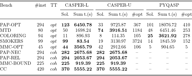
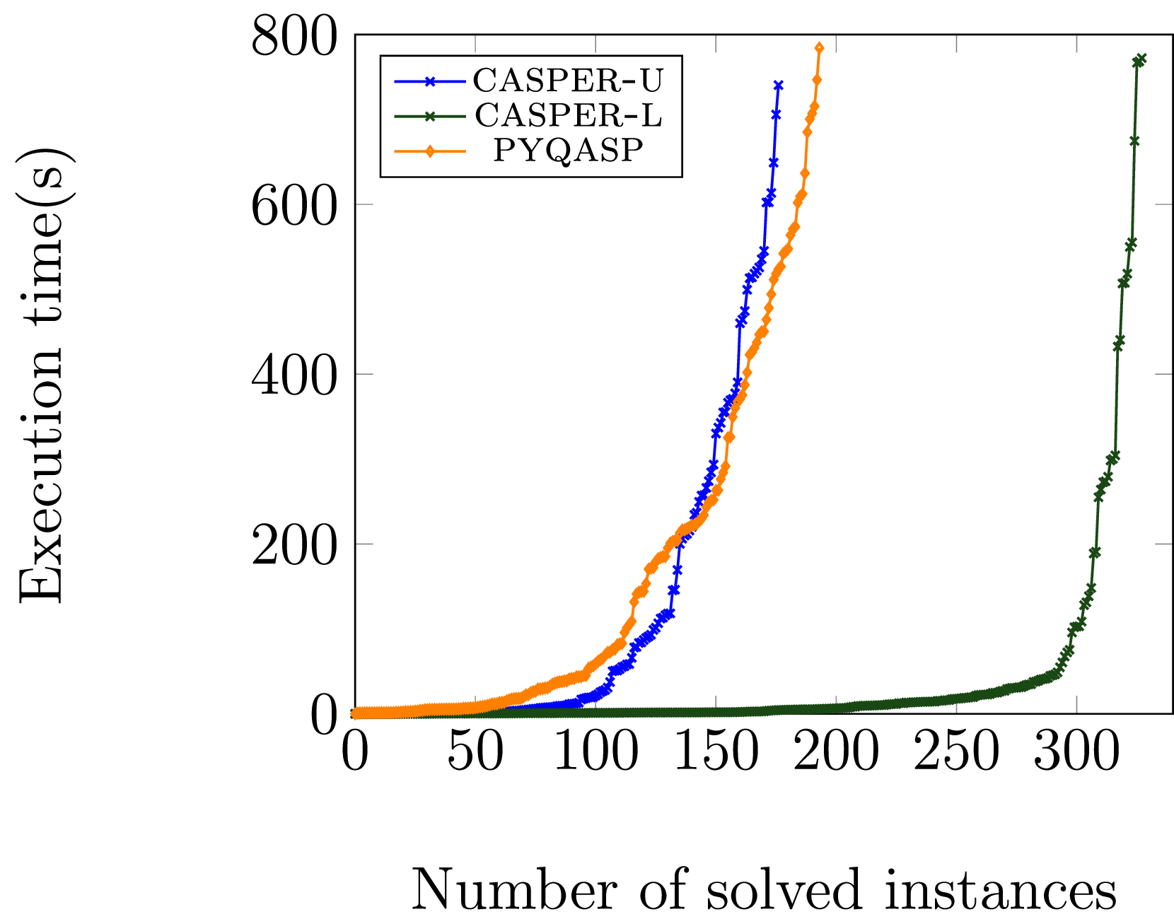
 opt
opt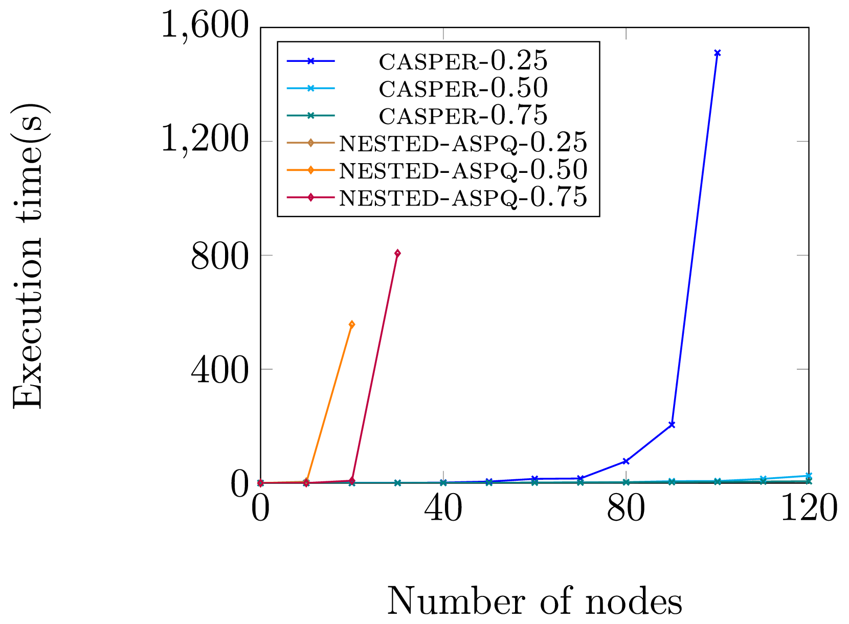


 Open access

