


1. Introduction
A classical question in singularity theory is to understand the complexity of the singularities of hypersurfaces. One invariant of hypersurface singularities is the log canonical threshold, which is determined by any resolution of the singularity. Log canonical thresholds appear in different problems pertaining to differential and algebraic geometry. For instance, the greatest root of the Bernstein polynomial is the negative of the log canonical threshold (see [Reference Kollár9, Theorem 10.6]). Another important application is in establishing the existence of Kähler–Einstein metrics on Fano varieties using Tian’s criterion, which is an asymptotic version of the log canonical threshold [Reference Tian17]. In this regard, log canonical thresholds play a role in stability problems (see e.g., [Reference Zanardini23]).
Log canonical thresholds were first known as complex singularity exponents. The log canonical threshold of a convergent power series $f \in \mathbb C\{x_1, \ldots , x_n\}$
can be defined as the supremum over real numbers
$f \in \mathbb C\{x_1, \ldots , x_n\}$
can be defined as the supremum over real numbers $\lambda$
such that the integral of
$\lambda$
such that the integral of $1/\left \lvert\ f \right \rvert ^{2\lambda }$
converges around
$1/\left \lvert\ f \right \rvert ^{2\lambda }$
converges around $\boldsymbol 0$
. The properties of log canonical thresholds have been studied with regards to the mixed Hodge structures of the vanishing cohomology (see, for instance, [Reference Steenbrink14, Reference Varčenko18]). This was then used in [Reference Steenbrink14] to define an invariant called the spectrum of an isolated hypersurface singularity, which was further generalised in [Reference Steenbrink16] to any hypersurface singularity. By [Reference Steenbrink16, Section 1], in the case of isolated hypersurface singularities, the spectral numbers of the singularity can be used to retrieve the Milnor number. By [Reference Varchenko19, Section 4] or [Reference Kollár9, Theorem 9.5], the log canonical threshold of
$\boldsymbol 0$
. The properties of log canonical thresholds have been studied with regards to the mixed Hodge structures of the vanishing cohomology (see, for instance, [Reference Steenbrink14, Reference Varčenko18]). This was then used in [Reference Steenbrink14] to define an invariant called the spectrum of an isolated hypersurface singularity, which was further generalised in [Reference Steenbrink16] to any hypersurface singularity. By [Reference Steenbrink16, Section 1], in the case of isolated hypersurface singularities, the spectral numbers of the singularity can be used to retrieve the Milnor number. By [Reference Varchenko19, Section 4] or [Reference Kollár9, Theorem 9.5], the log canonical threshold of $f$
is
$f$
is $\min (1, \beta _{\mathbb C(\ f)})$
, where
$\min (1, \beta _{\mathbb C(\ f)})$
, where $\beta _{\mathbb C(\ f)}$
is the complex singular index, and by [Reference Steenbrink15], the smallest spectral number in the spectral sequence is
$\beta _{\mathbb C(\ f)}$
is the complex singular index, and by [Reference Steenbrink15], the smallest spectral number in the spectral sequence is $\beta _{\mathbb C(\ f)} - 1$
.
$\beta _{\mathbb C(\ f)} - 1$
.
In this paper, we study log canonical thresholds of reduced plane curves $C \subset \mathbb{A}^2$
at a point
$C \subset \mathbb{A}^2$
at a point $P \in C$
, where reduced means that the defining polynomial of the curve is not divisible by the square of any non-unit polynomial. The pair
$P \in C$
, where reduced means that the defining polynomial of the curve is not divisible by the square of any non-unit polynomial. The pair $(\mathbb{A}^2, C)$
is said to be log canonical at
$(\mathbb{A}^2, C)$
is said to be log canonical at $P$
if it has a log resolution over
$P$
if it has a log resolution over $P$
such that locally the coefficients of all the prime divisors of the log pullback of
$P$
such that locally the coefficients of all the prime divisors of the log pullback of $C$
are at most
$C$
are at most $1$
(Definition 2.3). The log canonical threshold of
$1$
(Definition 2.3). The log canonical threshold of $C$
at
$C$
at $P$
is then given by
$P$
is then given by
 \begin{equation*} \operatorname {lct}_P(\mathbb{A}^2, C) \, :\!= \, \operatorname {sup} \left \{ \left .\lambda \in \mathbb Q_{\gt 0} \;\right |\; (\mathbb{A}^2, \lambda C)\, \text{is log canonical at the point}\,P \right \}. \end{equation*}
Log canonical threshold is roughly the reciprocal of multiplicity ([Reference Kollár9, Lemma 8.10.1] or [Reference Kollár, Smith and Corti10, Exercise 6.18 and Lemma 6.35]):
 \begin{equation} \frac {1}{\operatorname {mult}_P(C)} \leq \operatorname {lct}_P(\mathbb{A}^2, C) \leq \frac {2}{\operatorname {mult}_P(C)}. \end{equation}
Log canonical threshold is a finer invariant than multiplicity and Milnor number in the case of reduced plane curves of degree 5: there are five possible multiplicities (1–5), 16 possible Milnor numbers (0–14 and 16) and 24 possible log canonical thresholds (Table 1).
Log canonical thresholds of reduced plane curves

Equation (1.1) shows that a high multiplicity corresponds to a low log canonical threshold. To put it more sharply, by [Reference Cheltsov3, Theorem 4.1], the least log canonical threshold of a reduced plane curve of degree $d$
is
$d$
is $2/d$
, which happens precisely when the multiplicity at the point is
$2/d$
, which happens precisely when the multiplicity at the point is $d$
, implying that the curve is the union of
$d$
, implying that the curve is the union of $d$
lines. By [Reference Cheltsov4] or [Reference Viswanathan20, Proposition 4.5], if
$d$
lines. By [Reference Cheltsov4] or [Reference Viswanathan20, Proposition 4.5], if $\operatorname {mult}_P(C) \leq d-2$
, then
$\operatorname {mult}_P(C) \leq d-2$
, then
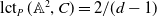
 $\operatorname {lct}_P(\mathbb A^2, C) \geq 2/(d-1)$
. Therefore, the lowest log canonical thresholds, meaning the values between
$\operatorname {lct}_P(\mathbb A^2, C) \geq 2/(d-1)$
. Therefore, the lowest log canonical thresholds, meaning the values between $2/d$
and
$2/d$
and $2/(d-1)$
, happen when the multiplicity at the point is high, meaning at least
$2/(d-1)$
, happen when the multiplicity at the point is high, meaning at least $d-1$
.
$d-1$
.
Our main result is giving a simple formula for the log canonical threshold of a reduced plane curve of degree $d$
at a point on the curve of multiplicity
$d$
at a point on the curve of multiplicity $d-1$
:
$d-1$
:
Theorem 1.1 (= Theorem3.2). Let $C$
be a reduced plane curve of degree
$C$
be a reduced plane curve of degree $d$
and
$d$
and $P$
a point of
$P$
a point of $C$
of multiplicity
$C$
of multiplicity $d-1$
. Let
$d-1$
. Let $C^1$
be the strict transform of
$C^1$
be the strict transform of $C$
under the blowup of the plane
$C$
under the blowup of the plane $\mathbb{A}^2$
at
$\mathbb{A}^2$
at $P$
and let
$P$
and let $E$
be the exceptional divisor. Then
$E$
be the exceptional divisor. Then
 \begin{equation*} \operatorname {lct}_P(\mathbb{A}^2, C) \lt \frac {2}{d-1} \iff \exists Q\in C^1\colon \operatorname {mult}_Q(C^1 \cdot E) \gt \frac {d-1}{2}. \end{equation*}
If the point $Q$
exists, then it is unique. In this case,
$Q$
exists, then it is unique. In this case,
 \begin{align*} \operatorname {lct}_P(\mathbb{A}^2, C) = \left \{\begin{aligned} & \frac {2 \cdot \operatorname {mult}_Q(C^1 \cdot E) - 1}{d \cdot (\operatorname {mult}_Q(C^1 \cdot E) - 1) + 1} && \begin{aligned} \textit{if} \,L_Q \,\text{is an irreducible}\\[2pt] \textit{component of}\,C, \end{aligned}\\[2pt] & \frac {2 \cdot \operatorname {mult}_Q(C^1 \cdot E) + 1}{d \cdot \operatorname {mult}_Q(C^1 \cdot E)} && \textit{otherwise}, \end{aligned}\right . \end{align*}
where $L_Q$
is the unique line on the affine plane containing
$L_Q$
is the unique line on the affine plane containing $P$
such that its strict transform contains
$P$
such that its strict transform contains $Q$
.
$Q$
.
It was proved in [Reference Cheltsov4, Theorem 1.10] that for $d \geq 4$
, the five smallest log canonical thresholds are
$d \geq 4$
, the five smallest log canonical thresholds are
 \begin{equation*} \left \{ \frac {2}{d}, \frac {2d-3}{(d-1)^2}, \frac {2d-1}{d(d-1)}, \frac {2d-5}{d^2-3d+1}, \frac {2d-3}{d(d-2)} \right \}, \end{equation*}
and in [Reference Viswanathan20, Theorem 1.8], that for $d \geq 5$
the sixth smallest log canonical threshold is
$d \geq 5$
the sixth smallest log canonical threshold is $\frac {2d - 7}{d^2 - 4d + 1}$
. A keen eye will notice a pattern in the six rational numbers above, namely that they contain two simple subsequences. We show that these subsequences can be extended. Moreover, we describe all log canonical thresholds at points of multiplicity
$\frac {2d - 7}{d^2 - 4d + 1}$
. A keen eye will notice a pattern in the six rational numbers above, namely that they contain two simple subsequences. We show that these subsequences can be extended. Moreover, we describe all log canonical thresholds at points of multiplicity $d-1$
:
$d-1$
:
Corollary 1.2 (= Corollary 3.5). Let $\Lambda _{d, d-1}$
denote the set of log canonical thresholds of pairs
$\Lambda _{d, d-1}$
denote the set of log canonical thresholds of pairs $(\mathbb A^2, C)$
at a point of multiplicity
$(\mathbb A^2, C)$
at a point of multiplicity $d-1$
of a reduced plane curve
$d-1$
of a reduced plane curve $C$
of degree
$C$
of degree $d$
. Then for every
$d$
. Then for every $d \geq 3$
,
$d \geq 3$
,
 \begin{align*} \begin{aligned} \Lambda _{d, d-1} = \left \{ \frac {2}{d-1} \right \} & \cup \left \{ \left .\dfrac {2k + 1}{kd + 1} \;\right |\; k \in \Bigl \{\bigl \lfloor \frac {d-1}{2}\bigr \rfloor , \ldots , d-2\Bigr \} \right \}\\[3pt] & \cup \left \{ \left .\dfrac {2k + 1}{kd} \;\right |\; k \in \Bigl \{\bigl \lfloor \frac {d+1}{2}\bigr \rfloor , \ldots , d-1\Bigr \} \right \}, \end{aligned} \end{align*}
where $\lfloor x\rfloor$
denotes the greatest integer not greater than
$\lfloor x\rfloor$
denotes the greatest integer not greater than $x$
.
$x$
.
Lastly, we concentrate on low-degree curves. Singularities of low-degree plane curves have been intensively studied from various points of view. We fill a gap in this direction by computing the log canonical thresholds for all reduced plane curves of degree at most $5$
. By [Reference Varchenko19], log canonical threshold is constant in
$5$
. By [Reference Varchenko19], log canonical threshold is constant in $\mu$
-constant strata (Definition 4.3), meaning that all the power series in a connected component of the set of power series with given Milnor number have the same log canonical threshold at the origin. Therefore, we use the existing classification lists of singularities to compute log canonical thresholds.
$\mu$
-constant strata (Definition 4.3), meaning that all the power series in a connected component of the set of power series with given Milnor number have the same log canonical threshold at the origin. Therefore, we use the existing classification lists of singularities to compute log canonical thresholds.
Table 1 gives an exhaustive list of all possible log canonical thresholds of reduced plane curves $C$
of degree at most
$C$
of degree at most $5$
at a given point
$5$
at a given point $P$
.
$P$
.
The paper is organised as follows. In Section 2, we set up the preliminary definitions and results that are needed to describe log canonical thresholds of reduced plane curves, such as the notion of power series and log resolutions. Section 3 is devoted towards proving Theorem1.1 (= Theorem3.2). In addition to this, we also provide the complete list of all possible values of log canonical thresholds that a pair $(\mathbb{A}^2,C)$
can take at a point
$(\mathbb{A}^2,C)$
can take at a point $p\in C$
of multiplicity
$p\in C$
of multiplicity $d-1$
in a curve
$d-1$
in a curve $C$
of degree
$C$
of degree $d$
. This is Corollary 3.5.
$d$
. This is Corollary 3.5.
Section 4 contains Table 2, which lists all the singularities that reduced plane curves of degree at most $5$
can have, and Table 3, which lists the normal forms and the log canonical thresholds for each singularity. It also contains the proofs for why the tables give an exhaustive list.
$5$
can have, and Table 3, which lists the normal forms and the log canonical thresholds for each singularity. It also contains the proofs for why the tables give an exhaustive list.
Singularities of reduced plane curves of given degree

Notation for normal forms

2. Preliminaries
Notation 2.1. To avoid possible misunderstanding, we list some of the standard notations we use.
-
(1) Variety – an integral separated scheme of finite type over the complex numbers $\mathbb C$
.
$\mathbb C$
. -
(2) Curve – a reduced, separated scheme of finite type over
$\mathbb C$
of pure dimension
$1$
. -
(3)
$\mathbb C\{x_1, \ldots , x_n\}$
– the
$\mathbb C$
-algebra of power series in variables
$x_1, \ldots , x_n$
that are absolutely convergent in a neighbourhood of the origin. -
(4)
$(\mathbb{V}(\ f), \boldsymbol 0)$
– the (possibly nonreduced) complex space subgerm of
$(\mathbb C^n, \boldsymbol 0)$
defined by
$f \in \mathbb C\{x_1, \ldots , x_n\}$
. -
(5)
$f$
is square-free – no square of a non-unit in
$\mathbb C[x_1, \ldots , x_n]$
divides
$f$
. -
(6) Plane curve of degree
$d$
– a scheme which is isomorphic to an open dense subscheme of
$\operatorname {Proj} \mathbb C[x, y, z] / (\ f)$
for a square-free polynomial
$f \in \mathbb C[x, y, z]$
homogeneous of degree
$d$
, where
$d$
is a positive integer.


Given a positive integer $n$
, a nonzero convergent power series
$n$
, a nonzero convergent power series $f \in \mathbb C\{x_1, \ldots , x_n\}$
and positive rational numbers
$f \in \mathbb C\{x_1, \ldots , x_n\}$
and positive rational numbers $(w_1, \ldots , w_n)$
called weights corresponding to the variables
$(w_1, \ldots , w_n)$
called weights corresponding to the variables $x_1, \ldots , x_n$
, we have the following notation:
$x_1, \ldots , x_n$
, we have the following notation:
-
(7)
$\operatorname {wt}(\ f)$
– the weight of
$f$
, defined by
\begin{align*} \operatorname {wt}(\ f) \, :\!= \, \min \left \{ \bigg. i_1 w_1 + \ldots + i_n w_n \;\bigg| \; \begin{aligned} & i_1, \ldots , i_n \in \mathbb Z_{\geq 0}, \text{the coefficient}\\ & \text{of} x_1^{i_1} \cdot \ldots \cdot x_n^{i_n}\, \text{in} \,f \,\text{is non-zero} \end{aligned} \right \}, \end{align*}
-
(8)
$\operatorname {mult}(\ f)$
– the multiplicity of
$f$
, defined to be the weight of
$f$
with respect to the weights
$(1, \ldots , 1)$
, -
(9)
$f$
is quasihomogeneous – all the monomials with a non-zero coefficient in
$f$
have the same weight, -
(10)
$f$
is semiquasihomogeneous – the nonzero quasihomogeneous subpolynomial of
$f$
that is of least weight (i.e.,, the sum of all the monomials of weight
$\operatorname {wt}(\ f)$
together with their coefficients in
$f$
) defines a smooth germ or an isolated singularity at the origin.


Given curves $C$
and
$C$
and $C'$
containing a closed point
$C'$
containing a closed point $P$
, we use the notation below:
$P$
, we use the notation below:
-
(11)
$\operatorname {mult}_P(C)$
– the multiplicity of
$C$
at
$P$
is defined to be
$\operatorname {mult}(\ f)$
, where
$f$
is any convergent power series in
$\mathbb C\{x, y\}$
such that the complex space germ
$(C^{\mathrm{an}}, P)$
is isomorphic to the complex space subgerm
$(\mathbb V(\ f), \boldsymbol 0)$
of
$(\mathbb C^2, \boldsymbol 0)$
, where
$C^{\mathrm{an}}$
denotes the analytification of
$C$
, -
(12)
$\operatorname {mult}_P(C \cdot C')$
– the intersection multiplicity of
$C$
and
$C'$
along
$P$
is defined in [Reference Fulton5, Definition 7.1] and can be computed using [Reference Fulton5, Example 7.1.10(b)].


2.1. Log resolutions
Below, we give the technical definitions of log resolution and the log pullback $D'$
of a divisor
$D'$
of a divisor $D$
. The characterising property of log pullback in the setting of Definition 2.2 is the linear equivalence
$D$
. The characterising property of log pullback in the setting of Definition 2.2 is the linear equivalence
 \begin{align*} K_{S'} + D' \sim \varphi ^*(K_S + D). \\[-25pt] \end{align*}
Definition 2.2 [Reference Kollár and Mori8, Notation 0.4]. Let $S$
be a smooth variety. A
$S$
be a smooth variety. A $\mathbb Q$
-
divisor
on
$\mathbb Q$
-
divisor
on $S$
is a formal
$S$
is a formal $\mathbb Q$
-linear combination
$\mathbb Q$
-linear combination $\sum \lambda _i D_i$
of prime divisors
$\sum \lambda _i D_i$
of prime divisors $D_i$
where
$D_i$
where $\lambda _i \in \mathbb Q$
. An effective
$\lambda _i \in \mathbb Q$
. An effective $\mathbb Z$
-divisor
$\mathbb Z$
-divisor $\sum \lambda _i D_i$
is
snc
if all the prime divisors
$\sum \lambda _i D_i$
is
snc
if all the prime divisors $D_i$
are smooth and around every point of
$D_i$
are smooth and around every point of $S$
,
$S$
, $\sum \lambda _i D_i$
is locally analytically given by
$\sum \lambda _i D_i$
is locally analytically given by $V(x_1^{a_1} \cdot \ldots \cdot x_n^{a_n})$
in
$V(x_1^{a_1} \cdot \ldots \cdot x_n^{a_n})$
in $\mathbb C^n$
where
$\mathbb C^n$
where $(a_1, \ldots , a_n) \in \mathbb Z_{\geq 0}^n$
.
$(a_1, \ldots , a_n) \in \mathbb Z_{\geq 0}^n$
.
Let $D$
be a
$D$
be a $\mathbb Q$
-divisor on a smooth variety
$\mathbb Q$
-divisor on a smooth variety $S$
. A
log resolution of
$S$
. A
log resolution of $(S, D)$
over
$(S, D)$
over $P$
is a proper birational morphism
$P$
is a proper birational morphism $\pi \colon S' \to S$
from a scheme
$\pi \colon S' \to S$
from a scheme $S'$
such that there exists an open neighbourhood
$S'$
such that there exists an open neighbourhood $U \subseteq S$
of
$U \subseteq S$
of $P$
such that
$P$
such that $\pi ^{-1}U$
is a smooth variety, the exceptional locus
$\pi ^{-1}U$
is a smooth variety, the exceptional locus $E$
of
$E$
of $\left .\pi \right |_{\pi ^{-1}U}$
is of pure codimension
$\left .\pi \right |_{\pi ^{-1}U}$
is of pure codimension $1$
and
$1$
and $E \cup \left .\pi \right |_{\pi ^{-1}U}^{-1}(\operatorname {Supp}(D \cap U))$
is an snc divisor of
$E \cup \left .\pi \right |_{\pi ^{-1}U}^{-1}(\operatorname {Supp}(D \cap U))$
is an snc divisor of $\pi ^{-1}U$
.
$\pi ^{-1}U$
.
For any proper birational morphism $\varphi \colon S' \to S$
from a smooth variety
$\varphi \colon S' \to S$
from a smooth variety $S'$
, the relative canonical divisor of
$S'$
, the relative canonical divisor of $\varphi$
, denoted
$\varphi$
, denoted $K_\varphi$
, is the unique
$K_\varphi$
, is the unique $\mathbb Q$
-divisor that is linearly equivalent to
$\mathbb Q$
-divisor that is linearly equivalent to $\varphi ^*(K_S) - K_{S'}$
and supported on the exceptional locus of
$\varphi ^*(K_S) - K_{S'}$
and supported on the exceptional locus of $\varphi$
, where
$\varphi$
, where $K_S$
and
$K_S$
and $K_{S'}$
are the canonical classes of
$K_{S'}$
are the canonical classes of $S$
and
$S$
and $S'$
, respectively. The
log pullback
of
$S'$
, respectively. The
log pullback
of $D$
with respect to
$D$
with respect to $\varphi$
is the
$\varphi$
is the $\mathbb Q$
-divisor
$\mathbb Q$
-divisor $D' = K_\varphi + \varphi ^* D$
on
$D' = K_\varphi + \varphi ^* D$
on $S'$
.
$S'$
.
Now we are ready to define the log canonical threshold.
Definition 2.3 ([Reference Kollár9, Definition 3.5] or [Reference Kollár and Mori8, Definition 2.34]). Let $D$
be a
$D$
be a $\mathbb Q$
-divisor on a smooth variety
$\mathbb Q$
-divisor on a smooth variety $S$
and let
$S$
and let $P \in S$
be a point. The pair
$P \in S$
be a point. The pair $(S, D)$
is log canonical at
$(S, D)$
is log canonical at $P$
if we can restrict
$P$
if we can restrict $(S, D)$
to an open neighbourhood of
$(S, D)$
to an open neighbourhood of $P$
such that there exists a log resolution with all the coefficients of the prime divisors in the log pullback of
$P$
such that there exists a log resolution with all the coefficients of the prime divisors in the log pullback of $D$
at most
$D$
at most $1$
. The
log canonical threshold of
$1$
. The
log canonical threshold of $(S, D)$
at
$(S, D)$
at $P$
is
$P$
is
 \begin{equation*} \operatorname {lct}_P(S, D) \, :\!= \, \operatorname {sup}\bigl \{ \lambda \in \mathbb Q_{\gt 0} \;\big |\; (S, \lambda D) \,\text{is log canonical at}\,P \bigr \}. \end{equation*}
Note that log canonical threshold at a closed point is a local analytic invariant [Reference Matsuki12, Proposition 4-4-4]. The following lemma is used to prove Theorem1.1 and to compute the log canonical thresholds of the polynomials in Table 3.
Lemma 2.4 ([Reference Kollár9, Propositions 8.13 and 8.14 and Remark 8.14.1] or [Reference Kuwata11], Proposition 2.1]). Let $f \in \mathbb C\{x_1, \ldots , x_n\}$
. Assign positive rational weights
$f \in \mathbb C\{x_1, \ldots , x_n\}$
. Assign positive rational weights $\boldsymbol w = (w_1, \ldots , w_n)$
to the variables. Let
$\boldsymbol w = (w_1, \ldots , w_n)$
to the variables. Let $f_w$
denote the weighted homogeneous leading term of
$f_w$
denote the weighted homogeneous leading term of $f$
. Define
$f$
. Define $b \, :\!= \, \sum _i w_i / \operatorname {wt}(\ f)$
. Considering
$b \, :\!= \, \sum _i w_i / \operatorname {wt}(\ f)$
. Considering $\mathbb C^n$
,
$\mathbb C^n$
, $\mathbb{V}(\ f)$
and
$\mathbb{V}(\ f)$
and $\mathbb{V}(\ f_{\boldsymbol w})$
as complex space germs around
$\mathbb{V}(\ f_{\boldsymbol w})$
as complex space germs around $\boldsymbol 0$
, we have
$\boldsymbol 0$
, we have $\operatorname {lct}_{\boldsymbol 0}(\mathbb C^n, \mathbb{V}(\ f)) \leq b$
. Moreover, if the pair
$\operatorname {lct}_{\boldsymbol 0}(\mathbb C^n, \mathbb{V}(\ f)) \leq b$
. Moreover, if the pair $(\mathbb C^n, b \mathbb{V}(\ f_w))$
is log canonical outside the origin, then
$(\mathbb C^n, b \mathbb{V}(\ f_w))$
is log canonical outside the origin, then $\operatorname {lct}_{\boldsymbol 0}(\mathbb C^n, \mathbb{V}(\ f)) = b$
.
$\operatorname {lct}_{\boldsymbol 0}(\mathbb C^n, \mathbb{V}(\ f)) = b$
.
2.2. Power series
We use the standard definitions below in Section 4.
Definition 2.5 [Reference Greuel, Lossen and Shustin6, Definitions I.1.1, I.1.47 and I.2.1]. Let $n$
be a positive integer. We denote by
$n$
be a positive integer. We denote by
-
•
$\mu (\ f)$
– the
Milnor number
of
$f \in \mathbb C\{x_1, \ldots , x_n\}$
, defined by
\begin{equation*} \mu (\ f) = \dim _\mathbb C \frac {\mathbb C\{x_1, \ldots , x_n\}}{(\frac {\partial f}{\partial x_1}, \ldots , \frac {\partial f}{\partial x_n})}. \end{equation*}


Definition 2.6 ([Reference Greuel, Lossen and Shustin6, Definition I.2.9] and [Reference Arnold, Gusein-Zade and Varchenko2, Introduction to Part II]). Let $n \leq m$
be positive integers. Let
$n \leq m$
be positive integers. Let $f, g \in \mathbb C\{x_1, \ldots , x_n\}$
and
$f, g \in \mathbb C\{x_1, \ldots , x_n\}$
and $h \in \mathbb C\{y_1, \ldots , y_m\}$
.
$h \in \mathbb C\{y_1, \ldots , y_m\}$
.
-
• We say that
$f$
and
$g$
are
right equivalent
if there exists an automorphism
$\Phi$
of
$\mathbb C\{x_1, \ldots , x_n\}$
such that
$\Phi (\ f) = g$
. In simpler terms,
$f$
and
$g$
are right equivalent if they coincide up to local analytic coordinate changes.
-
• We say that
$f$
and
$h$
are
stably right equivalent
if there exists a non-negative integer
$k$
and an isomorphism
$\Psi \colon \mathbb C\{x_1, \ldots , x_{n+k}\} \to \mathbb C\{y_1, \ldots , y_{n+k}\}$
such that
$\Psi (\ f + x_{n+1}^2 + \ldots + x_{n+k}^2) = h + y_{m+1}^2 + \ldots + y_{n+k}^2$
.


Remark 2.7. Normal forms of singularities are often considered up to stable right equivalence. So, while the power series $x^3 + y^6 + z^2 + 2 xyz$
defines a surface singularity, it is stably right equivalent to the power series
$x^3 + y^6 + z^2 + 2 xyz$
defines a surface singularity, it is stably right equivalent to the power series $x^2 y^2 + x^3 + y^6$
, which defines a curve singularity. Due to this, there are several different notations for the same singularity class (Remark 4.4(c)). Note that if the number of variables is the same, then two power series
$x^2 y^2 + x^3 + y^6$
, which defines a curve singularity. Due to this, there are several different notations for the same singularity class (Remark 4.4(c)). Note that if the number of variables is the same, then two power series $f, g \in \mathbb C\{x_1, \ldots , x_n\}$
are stably right equivalent if and only if they are right equivalent, see [Reference Arnold, Gusein-Zade and Varchenko2, Remark in Section 11.1].
$f, g \in \mathbb C\{x_1, \ldots , x_n\}$
are stably right equivalent if and only if they are right equivalent, see [Reference Arnold, Gusein-Zade and Varchenko2, Remark in Section 11.1].
3. High multiplicity curves
In this section, we classify log canonical thresholds at points of multiplicity $d-1$
for reduced plane curves of degree
$d-1$
for reduced plane curves of degree $d$
. The notation we use is given in Setting 3.1.
$d$
. The notation we use is given in Setting 3.1.
Setting 3.1. Let $d \geq 3$
be an integer. Let
$d \geq 3$
be an integer. Let $P$
be a point of a reduced affine plane curve
$P$
be a point of a reduced affine plane curve $C$
of degree
$C$
of degree $d$
such that
$d$
such that $\operatorname {mult}_P C = d-1$
. Let
$\operatorname {mult}_P C = d-1$
. Let $C^1$
be the strict transform of
$C^1$
be the strict transform of $C$
under the blowup of the affine plane along
$C$
under the blowup of the affine plane along $P$
with exceptional divisor
$P$
with exceptional divisor $E_1$
. For every point
$E_1$
. For every point $Q \in C^1$
such that
$Q \in C^1$
such that $\operatorname {mult}_Q(C^1 \cdot E_1) \gt 1$
, let
$\operatorname {mult}_Q(C^1 \cdot E_1) \gt 1$
, let $L_Q$
be the line on the affine plane through
$L_Q$
be the line on the affine plane through $P$
such that its strict transform passes through
$P$
such that its strict transform passes through $Q$
. For every such
$Q$
. For every such $Q \in C^1$
, let
$Q \in C^1$
, let $C_Q^1$
be the strict transform of the Zariski closure
$C_Q^1$
be the strict transform of the Zariski closure $C_Q$
of
$C_Q$
of $C \setminus L_Q$
. Define the positive integer
$C \setminus L_Q$
. Define the positive integer $k_Q$
by
$k_Q$
by
 \begin{equation*} k_Q \, :\!= \, \operatorname {mult}_Q(C_Q^1 \cdot E_1) \end{equation*}
and define the positive rational number $l_Q$
by
$l_Q$
by
 \begin{align*} l_Q \, :\!= \, \left \{\begin{aligned} \dfrac {2 k_Q + 1}{k_Q d + 1} & \quad \text{if} \,L_Q \,\text{is an irreducible component of} \,C,\\[3pt] \dfrac {2 k_Q + 1}{k_Q d} & \quad \text{otherwise}. \end{aligned}\right . \end{align*}
By equation (1.1), $\operatorname {lct}_P(\mathbb{A}^2, C) \leq 2/(d-1)$
. The main theorem of this section is as follows:
$\operatorname {lct}_P(\mathbb{A}^2, C) \leq 2/(d-1)$
. The main theorem of this section is as follows:
Theorem 3.2. With the notations and setup as in Setting 3.1 ,
 \begin{equation*} \operatorname {lct}_P(\mathbb{A}^2, C) \lt \frac {2}{d-1} \iff \exists Q\in C^1\colon \operatorname {mult}_Q(C^1 \cdot E_1) \gt \frac {d-1}{2}. \end{equation*}
Moreover, if the point $Q$
exists, then it is unique and
$Q$
exists, then it is unique and $\operatorname {lct}_P(\mathbb{A}^2, C) = l_Q$
.
$\operatorname {lct}_P(\mathbb{A}^2, C) = l_Q$
.
To prove Theorem3.2, we first describe $C$
using equations:
$C$
using equations:
Lemma 3.3.
We say that two triples $(C, P, Q)$
and
$(C, P, Q)$
and $(C', P', Q')$
are isomorphic if there exists an isomorphism
$(C', P', Q')$
are isomorphic if there exists an isomorphism $C \to C'$
of curves that takes the point
$C \to C'$
of curves that takes the point $P$
to
$P$
to $P'$
and
$P'$
and $Q$
to
$Q$
to $Q'$
. Let
$Q'$
. Let $\operatorname {Spec} \mathbb C[x_1, y] \cong \operatorname {Spec} \mathbb C[x/y, y] \gets \mathbb C[x, y]$
be one of the affine opens of the blowup of
$\operatorname {Spec} \mathbb C[x_1, y] \cong \operatorname {Spec} \mathbb C[x/y, y] \gets \mathbb C[x, y]$
be one of the affine opens of the blowup of $\mathbb A^2 \, :\!= \, \operatorname {Spec} \mathbb C[x, y]$
at
$\mathbb A^2 \, :\!= \, \operatorname {Spec} \mathbb C[x, y]$
at $\boldsymbol 0$
. Then, up to isomorphism, the triples
$\boldsymbol 0$
. Then, up to isomorphism, the triples $(C, P, Q)$
in Setting 3.1 are precisely given by
$(C, P, Q)$
in Setting 3.1 are precisely given by
 \begin{align*} \begin{aligned} C & = \mathbb V(\ f) \subseteq \mathbb A^2,\\[3pt] P & = \boldsymbol 0 \in \mathbb A^2,\\[3pt] Q & = \boldsymbol 0 \in \operatorname {Spec} \mathbb C[x_1, y], \end{aligned} \end{align*}
where $d \in \mathbb Z_{\geq 3}$
,
$d \in \mathbb Z_{\geq 3}$
, $a_i, b_{\ j\,} \in \mathbb C$
,
$a_i, b_{\ j\,} \in \mathbb C$
, $a_{k_Q} \neq 0$
,
$a_{k_Q} \neq 0$
, $b_0 \neq 0$
,
$b_0 \neq 0$
, $f$
is square-free and where one of the following holds
$f$
is square-free and where one of the following holds
-
•
$L_Q$
is an irreducible component of
$C$
,
$k_Q \in \{1, \ldots , d - 2\}$
and
or
\begin{equation*} f \, :\!= \, x \left ( \sum _{i\in \{k_Q,\, k_Q + 1,\, \ldots ,\, d-2\}} a_i x^i y^{d-2-i} + \sum _{\ j \in \{0,\, 1,\, \ldots ,\, d-1\}} b_{\ j\,} x^{\ j} y^{d-1-j} \right ), \end{equation*}
-
•
$L_Q$
is not an irreducible component of
$C$
,
$k_Q \in \{2, \ldots , d - 1\}$
and
\begin{equation*} f \, :\!= \, \sum _{i\in \{k_Q,\, k_Q + 1,\, \ldots ,\, d-1\}} a_i x^i y^{d-1-i} + \sum _{\ j \in \{0,\, 1,\, \ldots ,\, d\}} b_{\ j\,} x^{\ j} y^{d-j}. \end{equation*}


In both cases, $L_Q$
and
$L_Q$
and $E_1 \cap \operatorname {Spec} \mathbb C[x_1, y]$
from Setting 3.1 correspond, respectively, to
$E_1 \cap \operatorname {Spec} \mathbb C[x_1, y]$
from Setting 3.1 correspond, respectively, to $\mathbb V(x) \subseteq \mathbb A^2$
and
$\mathbb V(x) \subseteq \mathbb A^2$
and $\mathbb V(y) \subseteq \operatorname {Spec} \mathbb C[x_1, y]$
.
$\mathbb V(y) \subseteq \operatorname {Spec} \mathbb C[x_1, y]$
.
Proof.
We show how every $(C, P, Q)$
from Setting 3.1 is given by some
$(C, P, Q)$
from Setting 3.1 is given by some $(\mathbb V(\ f), \boldsymbol 0, \boldsymbol 0)$
. First, translate
$(\mathbb V(\ f), \boldsymbol 0, \boldsymbol 0)$
. First, translate $P$
to
$P$
to $\boldsymbol 0$
on
$\boldsymbol 0$
on $\mathbb A^2$
. Then use a linear invertible map on
$\mathbb A^2$
. Then use a linear invertible map on $\mathbb A^2$
fixing
$\mathbb A^2$
fixing $\boldsymbol 0$
to move
$\boldsymbol 0$
to move $Q$
to
$Q$
to $\boldsymbol 0 \in \operatorname {Spec} \mathbb C[x_1, y]$
. It follows that
$\boldsymbol 0 \in \operatorname {Spec} \mathbb C[x_1, y]$
. It follows that $L_Q = \mathbb V(x)$
and
$L_Q = \mathbb V(x)$
and $E_1 \cap \operatorname {Spec} \mathbb C[x_1, y] = \mathbb V(y)$
. The curve
$E_1 \cap \operatorname {Spec} \mathbb C[x_1, y] = \mathbb V(y)$
. The curve $C$
is given by
$C$
is given by $\mathbb V(g) \subseteq \mathbb A^2$
where
$\mathbb V(g) \subseteq \mathbb A^2$
where $g = g_{d-1} + g_d \in \mathbb C[x, y]$
, where
$g = g_{d-1} + g_d \in \mathbb C[x, y]$
, where $g_{d-1}$
and
$g_{d-1}$
and $g_d$
are respectively homogeneous of degrees
$g_d$
are respectively homogeneous of degrees $d-1$
and
$d-1$
and $d$
. The curve
$d$
. The curve $C^1 \cap \operatorname {Spec} \mathbb C[x_1, y]$
is given by
$C^1 \cap \operatorname {Spec} \mathbb C[x_1, y]$
is given by $g_{d-1}(x_1, 1) + y g_d(x_1, 1)$
. We see that
$g_{d-1}(x_1, 1) + y g_d(x_1, 1)$
. We see that $C^1 \cdot E = \operatorname {mult} g_{d-1}(x_1, 1)$
. This shows that
$C^1 \cdot E = \operatorname {mult} g_{d-1}(x_1, 1)$
. This shows that $g$
is equal to
$g$
is equal to $f$
for some choice of
$f$
for some choice of $a_i$
and
$a_i$
and $b_{\ j\,}$
.
$b_{\ j\,}$
.
Conversely, if $(C, P, Q)$
are given by some
$(C, P, Q)$
are given by some $(\mathbb V(\ f), \boldsymbol 0, \boldsymbol 0)$
as above, then
$(\mathbb V(\ f), \boldsymbol 0, \boldsymbol 0)$
as above, then $C$
is a reduced affine plane curve of degree
$C$
is a reduced affine plane curve of degree $d$
,
$d$
, $P \in C$
a point of multiplicity
$P \in C$
a point of multiplicity $d-1$
,
$d-1$
, $\operatorname {mult}_Q(C_Q^1 \cdot E_1) = k_Q$
and
$\operatorname {mult}_Q(C_Q^1 \cdot E_1) = k_Q$
and $\operatorname {mult}_Q(C^1 \cdot E_1) \gt 1$
.
$\operatorname {mult}_Q(C^1 \cdot E_1) \gt 1$
.
Proof of Theorem
3.2
. First, it is easy to compute that for any point $Q$
,
$Q$
, $l_Q \lt 2/(d-1)$
if and only if
$l_Q \lt 2/(d-1)$
if and only if $\operatorname {mult}_Q(C^1 \cdot E_1) \gt (d-1)/2$
. If such a point
$\operatorname {mult}_Q(C^1 \cdot E_1) \gt (d-1)/2$
. If such a point $Q$
exists, then it is necessarily unique since
$Q$
exists, then it is necessarily unique since
 \begin{equation*} \sum _{Q \in C^1 \cap E_1} \operatorname {mult}_Q(C^1 \cdot E_1) = C^1 \cdot E_1 = \operatorname {mult}_P(C) = d-1. \end{equation*}
Below, we construct explicit log resolutions of $(\mathbb A^2, C)$
over the point
$(\mathbb A^2, C)$
over the point $P$
to then obtain the value of
$P$
to then obtain the value of $\operatorname {lct}_P(\mathbb A^2, C)$
. Let
$\operatorname {lct}_P(\mathbb A^2, C)$
. Let $\pi _1\colon S_1 \to \mathbb{A}^2$
be the blowup along
$\pi _1\colon S_1 \to \mathbb{A}^2$
be the blowup along $P$
. If for every point
$P$
. If for every point $Q \in C^1 \cap E_1$
we have that
$Q \in C^1 \cap E_1$
we have that $\operatorname {mult}_Q(C^1 \cdot E_1) = 1$
, then
$\operatorname {mult}_Q(C^1 \cdot E_1) = 1$
, then $\operatorname {lct}_P(\mathbb{A}^2, C) = 2/(d-1)$
. Otherwise, let
$\operatorname {lct}_P(\mathbb{A}^2, C) = 2/(d-1)$
. Otherwise, let $Q$
be any point of
$Q$
be any point of $C^1$
such that
$C^1$
such that $\operatorname {mult}_Q(C^1 \cdot E_1) \gt 1$
. By Lemma 3.3,
$\operatorname {mult}_Q(C^1 \cdot E_1) \gt 1$
. By Lemma 3.3, $C_Q^1 \cap \operatorname {Spec} \mathbb C[x_1, y]$
is given by
$C_Q^1 \cap \operatorname {Spec} \mathbb C[x_1, y]$
is given by
 \begin{equation} f_1 \, :\!= \, \sum _{i\in \{k_Q,\, k_Q + 1,\, \ldots ,\, d-2\}} a_i x_1^i + y \sum _{\ j \in \{0,\, 1,\, \ldots ,\, d-1\}} b_{\ j\,} x_1^{\ j}, \end{equation}
if $L_Q$
is an irreducible component of
$L_Q$
is an irreducible component of $C$
and by
$C$
and by
 \begin{equation} f_1 \, :\!= \, \sum _{i\in \{k_Q,\, k_Q + 1,\, \ldots ,\, d-1\}} a_i x_1^i + y \sum _{\ j \in \{0,\, 1,\, \ldots ,\, d\}} b_{\ j\,} x_1^{\ j}. \end{equation}
otherwise. Every irreducible component of $C$
that is not a line has degree strictly greater than its multiplicity at
$C$
that is not a line has degree strictly greater than its multiplicity at $P$
. Therefore, the curve
$P$
. Therefore, the curve $C$
has exactly one irreducible component, which is not a line. Therefore,
$C$
has exactly one irreducible component, which is not a line. Therefore, $C_Q^1$
has exactly one irreducible component passing through
$C_Q^1$
has exactly one irreducible component passing through $Q$
. The strict transform
$Q$
. The strict transform $L_Q^1$
of
$L_Q^1$
of $L_Q$
under
$L_Q$
under $\pi _1$
is given on
$\pi _1$
is given on $\operatorname {Spec} \mathbb C[x_1, y]$
by
$\operatorname {Spec} \mathbb C[x_1, y]$
by $\mathbb V(x_1)$
. Using equations (3.1) and (3.2), we see that
$\mathbb V(x_1)$
. Using equations (3.1) and (3.2), we see that $L_Q^1$
and
$L_Q^1$
and $C_Q^1$
intersect in exactly one point, namely
$C_Q^1$
intersect in exactly one point, namely $Q$
, and the intersection is transversal. In particular,
$Q$
, and the intersection is transversal. In particular, $Q$
is a smooth point of
$Q$
is a smooth point of $C_Q^1$
.
$C_Q^1$
.
For every rational number $\lambda \gt 1/(d-1)$
, let
$\lambda \gt 1/(d-1)$
, let $D_\lambda$
denote the effective
$D_\lambda$
denote the effective $\mathbb Q$
-divisor
$\mathbb Q$
-divisor
 \begin{equation*} D_\lambda \, :\!= \, \lambda C^1 + (\lambda (d-1) - 1) E_1 \end{equation*}
on $S_1$
. Then
$S_1$
. Then $D_\lambda$
is the log pullback of
$D_\lambda$
is the log pullback of $\lambda C$
under
$\lambda C$
under $\pi _1$
.
$\pi _1$
.
We describe a log resolution $\pi _2 \circ \ldots \circ \pi _{k_Q + 1}$
over
$\pi _2 \circ \ldots \circ \pi _{k_Q + 1}$
over $Q$
of
$Q$
of $(S_1, D_\lambda )$
. Let
$(S_1, D_\lambda )$
. Let $\pi _2\colon S_2 \to S_1$
be the blowup along
$\pi _2\colon S_2 \to S_1$
be the blowup along $Q$
. For every
$Q$
. For every $r \in \{2, \ldots , k_Q\}$
, let
$r \in \{2, \ldots , k_Q\}$
, let $\pi _{r+1}\colon S_{r+1} \to S_r$
be the blowup along the point
$\pi _{r+1}\colon S_{r+1} \to S_r$
be the blowup along the point $Q_r \, :\!= \, \mathbb{V}(x_1, y_r)$
of the affine open
$Q_r \, :\!= \, \mathbb{V}(x_1, y_r)$
of the affine open $\operatorname {Spec} \mathbb C[x_1, y_r] \cong \operatorname {Spec} \mathbb C[x_1, y_{r-1}/x_1]$
of
$\operatorname {Spec} \mathbb C[x_1, y_r] \cong \operatorname {Spec} \mathbb C[x_1, y_{r-1}/x_1]$
of $S_r$
, where
$S_r$
, where $y_1 \, :\!= \, y$
. Let
$y_1 \, :\!= \, y$
. Let $C_Q^r$
denote the strict transform of
$C_Q^r$
denote the strict transform of $C_Q$
under
$C_Q$
under $\pi _1 \circ \ldots \circ \pi _r$
. We see using equations (3.1) and (3.2) that
$\pi _1 \circ \ldots \circ \pi _r$
. We see using equations (3.1) and (3.2) that $C_Q^r \cap \operatorname {Spec} \mathbb C[x_1, y_r]$
is given by
$C_Q^r \cap \operatorname {Spec} \mathbb C[x_1, y_r]$
is given by
 \begin{equation} f_r \, :\!= \, \sum _{i\in \{k_Q,\, k_Q + 1,\, \ldots ,\, d-2\}} a_i x_1^{i-r+1} + y_r \sum _{\ j \in \{0,\, 1,\, \ldots ,\, d-1\}} b_{\ j\,} x_1^{\ j}, \end{equation}
if $L_Q$
is an irreducible component of
$L_Q$
is an irreducible component of $C$
and by
$C$
and by
 \begin{equation} f_r \, :\!= \, \sum _{i\in \{k_Q,\, k_Q + 1,\, \ldots ,\, d-1\}} a_i x_1^{i-r+1} + y_r \sum _{\ j \in \{0,\, 1,\, \ldots ,\, d\}} b_{\ j\,} x_1^{\ j}. \end{equation}
otherwise. Let $E_r$
be the exceptional divisor of
$E_r$
be the exceptional divisor of $\pi _r$
and let
$\pi _r$
and let $E_i^r$
be the strict transform of the exceptional divisor of
$E_i^r$
be the strict transform of the exceptional divisor of $\pi _i$
under
$\pi _i$
under $\pi _i \circ \ldots \circ \pi _r$
. We have
$\pi _i \circ \ldots \circ \pi _r$
. We have
 \begin{align*} \begin{aligned} E_r \cap \operatorname {Spec} \mathbb C[x_1, y_r] & = \mathbb{V}(x_1),\\[3pt] E_1^r \cap \operatorname {Spec} \mathbb C[x_1, y_r] & = \mathbb{V}(y_r). \end{aligned} \end{align*}
We find that $E_r$
and
$E_r$
and $E_1^r$
intersect in exactly one point, namely
$E_1^r$
intersect in exactly one point, namely $Q_r$
, and the intersection is transversal. Moreover,
$Q_r$
, and the intersection is transversal. Moreover, $Q_r \notin E_2^r \cup E_3^r \cup \ldots \cup E_{r-1}^r$
and therefore,
$Q_r \notin E_2^r \cup E_3^r \cup \ldots \cup E_{r-1}^r$
and therefore, $\sum _{i \in \{1, \ldots , r\}} E_i^r$
is snc. Using equations (3.3) and (3.4), we see that
$\sum _{i \in \{1, \ldots , r\}} E_i^r$
is snc. Using equations (3.3) and (3.4), we see that $C_Q^r$
and
$C_Q^r$
and $E_r$
intersect in exactly one point, namely
$E_r$
intersect in exactly one point, namely $Q_r$
, and the intersection is transversal. Therefore,
$Q_r$
, and the intersection is transversal. Therefore, $(E_2^r \cup E_3^r \cup \ldots \cup E_{r-1}^r) \cap C_Q^r$
is empty. From equations (3.3) and (3.4), we find
$(E_2^r \cup E_3^r \cup \ldots \cup E_{r-1}^r) \cap C_Q^r$
is empty. From equations (3.3) and (3.4), we find
 \begin{equation*} \operatorname {mult}_{Q_r}(C_Q^r \cdot E_1^r) = k_Q - r + 1. \end{equation*}
The varieties $C_Q^{k_Q}$
,
$C_Q^{k_Q}$
, $E_{k_Q}$
and
$E_{k_Q}$
and $E_1^{k_Q}$
have pairwise transversal intersections at
$E_1^{k_Q}$
have pairwise transversal intersections at $Q_{k_Q}$
. Therefore,
$Q_{k_Q}$
. Therefore, $\pi _2 \circ \ldots \circ \pi _{k_Q + 1}$
is a log resolution of
$\pi _2 \circ \ldots \circ \pi _{k_Q + 1}$
is a log resolution of $(S_1, D_\lambda )$
over
$(S_1, D_\lambda )$
over $Q$
.
$Q$
.
Let $D_\lambda ^{k_Q + 1}$
denote the strict transform of
$D_\lambda ^{k_Q + 1}$
denote the strict transform of $D_\lambda$
under
$D_\lambda$
under $\pi _2 \circ \ldots \circ \pi _{k_Q + 1}$
. The log pullback of
$\pi _2 \circ \ldots \circ \pi _{k_Q + 1}$
. The log pullback of $D_\lambda$
under the composition
$D_\lambda$
under the composition $\pi _2 \circ \ldots \circ \pi _{k_Q + 1}$
is given by
$\pi _2 \circ \ldots \circ \pi _{k_Q + 1}$
is given by
 \begin{equation*} D_\lambda ^{k_Q + 1} + \sum _{\ j \in \{1, \ldots , k_Q\}} (\lambda (\ jd + 1) - 2j) E_{\ j+1}^{k_Q + 1} \end{equation*}
if $L_Q$
is an irreducible component of
$L_Q$
is an irreducible component of $C$
and
$C$
and
 \begin{equation*} D_\lambda ^{k_Q + 1} + \sum _{\ j \in \{1, \ldots , k_Q\}} (\lambda jd - 2j) E_{\ j+1}^{k_Q + 1} \end{equation*}
otherwise.
We have the following equivalences:
 \begin{align*} \begin{aligned} \lambda (d-1) - 1 & \leq 1 & \iff \,\, \lambda & \leq \frac {2}{d - 1},\\[2pt] \lambda (\, jd + 1) - 2j & \leq 1 & \iff \,\, \lambda & \leq \frac {2j + 1}{jd + 1},\\[2pt] \lambda jd - 2j & \leq 1 & \iff \,\, \lambda & \leq \frac {2j + 1}{jd}. \end{aligned} \end{align*}
Note that
 \begin{align*} l_Q = \left \{\begin{aligned} \min \left \{ \left .\frac {2j+1}{jd+1} \;\right |\; j \in \{1, \ldots , k_Q\} \right \} & \quad \begin{aligned} \text{if} \,L_Q \,\text{is an irreducible}\\[2pt] \text{component of}\,C, \end{aligned}\\[2pt] \min \left \{ \left .\frac {2j+1}{jd} \;\right |\; j \in \{1, \ldots , k_Q\} \right \} & \quad \text{otherwise}. \end{aligned}\right . \end{align*}
Let $\pi$
be the composition of the blowup
$\pi$
be the composition of the blowup $\pi _1$
with the
$\pi _1$
with the $\sum _Q k_Q$
blowups above, where the sum is over points
$\sum _Q k_Q$
blowups above, where the sum is over points $Q \in C^1$
such that
$Q \in C^1$
such that $\operatorname {mult}_Q(C^1 \cdot E_1) \gt 1$
. Then
$\operatorname {mult}_Q(C^1 \cdot E_1) \gt 1$
. Then $\pi$
is a log resolution of
$\pi$
is a log resolution of $(\mathbb{A}^2, C)$
over
$(\mathbb{A}^2, C)$
over $P$
. The log canonical threshold of
$P$
. The log canonical threshold of $(\mathbb{A}^2, C)$
at
$(\mathbb{A}^2, C)$
at $P$
is by definition the greatest positive rational number
$P$
is by definition the greatest positive rational number $\lambda$
such that all the coefficients of the prime divisors in the log pullback of
$\lambda$
such that all the coefficients of the prime divisors in the log pullback of $\lambda C$
with respect to
$\lambda C$
with respect to $\pi$
are at most
$\pi$
are at most $1$
. Therefore,
$1$
. Therefore,
 \begin{equation*} \operatorname {lct}_P(\mathbb{A}^2, C) = \min \left ( \left \{\dfrac {2}{d-1}\right \} \cup \left \{ \left .l_Q \;\right |\; Q \in C^1,\, \operatorname {mult}_Q(C^1 \cdot E_1) \gt 1 \right \} \right ). \end{equation*}
Remark 3.4. Theorem 3.2 can also be proved using a sequence of blowups at points and inversion of adjunction, similarly to the proofs of [ Reference Cheltsov4, Theorem 1.10] and [ Reference Viswanathan20, Theorem 1.8], or using the Newton polyhedron of the defining polynomial, see [ Reference Paemurru13, Theorem 3.10].
The method adopted in this paper works by giving very explicit equations to the curves under consideration, thus providing an intuition for the patterns of degrees of curves observed upon different blowups and the computations of log canonical thresholds at the points of blowup.
Corollary 3.5.
Let $\Lambda _{d, d-1}$
denote the set of log canonical thresholds of pairs
$\Lambda _{d, d-1}$
denote the set of log canonical thresholds of pairs $(\mathbb A^2, C)$
at a point of multiplicity
$(\mathbb A^2, C)$
at a point of multiplicity $d-1$
of a reduced plane curve
$d-1$
of a reduced plane curve $C$
of degree
$C$
of degree $d$
. Then for every
$d$
. Then for every $d \geq 3$
,
$d \geq 3$
,
 \begin{equation} \begin{aligned} \Lambda _{d, d-1} = \left \{ \frac {2}{d-1} \right \} & \cup \left \{ \left .\dfrac {2k + 1}{kd + 1} \;\right |\; k \in \Bigl \{\bigl \lfloor \frac {d-1}{2}\bigr \rfloor , \ldots , d-2\Bigr \} \right \}\\[3pt] & \cup \left \{ \left .\dfrac {2k + 1}{kd} \;\right |\; k \in \Bigl \{\bigl \lfloor \frac {d+1}{2}\bigr \rfloor , \ldots , d-1\Bigr \} \right \}, \end{aligned} \end{equation}
where $\lfloor x\rfloor$
denotes the greatest integer not greater than
$\lfloor x\rfloor$
denotes the greatest integer not greater than $x$
.
$x$
.
Proof.
If $f \in \mathbb C[x, y]$
is a multiplicity
$f \in \mathbb C[x, y]$
is a multiplicity $d-1$
polynomial such that its homogeneous degree
$d-1$
polynomial such that its homogeneous degree $d-1$
part is square-free, then
$d-1$
part is square-free, then $\operatorname {lct}_{\boldsymbol 0}(\mathbb A^2, V(\ f)) = 2/(d-1)$
. This shows that
$\operatorname {lct}_{\boldsymbol 0}(\mathbb A^2, V(\ f)) = 2/(d-1)$
. This shows that $2/(d-1) \in \Lambda _{d, d-1}$
.
$2/(d-1) \in \Lambda _{d, d-1}$
.
In Setting 3.1 by Theorem3.2, we have
 \begin{equation} \operatorname {lct}_P(\mathbb A^2, C) \leq 2/(d-1) \end{equation}
and the strict inequality holds in equation (3.6) if and only if there exists a point $Q \in C^1$
such that
$Q \in C^1$
such that $\operatorname {mult}_Q(C^1 \cdot E_1) \gt 1$
one of the following holds:
$\operatorname {mult}_Q(C^1 \cdot E_1) \gt 1$
one of the following holds:
 \begin{align}k_Q \geq \lfloor (d-1)/2\rfloor \,{\rm and} \,L_Q \,\text{is an irreducible component of}\, C,\,\text{or} \\[-26pt] \nonumber \end{align}
 \begin{equation}k_Q \geq \lfloor (d+1)/2\rfloor \,{\rm and} \,L_Q \,\text{is not an irreducible component of}\, C.\end{equation}
Moreover, if (3.7) or (3.8) holds for some $Q \in C^1$
, then
$Q \in C^1$
, then $\operatorname {lct}_P(\mathbb A^2, C) = l_Q$
. Denoting the right-hand side of equation (3.5) by
$\operatorname {lct}_P(\mathbb A^2, C) = l_Q$
. Denoting the right-hand side of equation (3.5) by $\mathrm{RHS}$
, we find
$\mathrm{RHS}$
, we find $\Lambda _{d, d-1} \subseteq \mathrm{RHS}$
. On the other hand, it is easy to construct examples of reduced plane curves satisfying (3.7) or (3.8) using Lemma 3.3. This proves that
$\Lambda _{d, d-1} \subseteq \mathrm{RHS}$
. On the other hand, it is easy to construct examples of reduced plane curves satisfying (3.7) or (3.8) using Lemma 3.3. This proves that $\mathrm{RHS} \subseteq \Lambda _{d, d-1}$
.
$\mathrm{RHS} \subseteq \Lambda _{d, d-1}$
.
Remark 3.6. The sets
 \begin{equation} \left \{ \left .\dfrac {2k + 1}{kd + 1} \;\right |\; k \in \Bigl \{\bigl \lfloor \frac {d-1}{2}\bigr \rfloor , \ldots , d-2\Bigr \} \right \} \end{equation}
and
 \begin{equation*} \left \{ \left .\dfrac {2k + 1}{kd} \;\right |\; k \in \Bigl \{\bigl \lfloor \frac {d+1}{2}\bigr \rfloor , \ldots , d-1\Bigr \} \right \} \end{equation*}
that appear in Corollary 3.5 are disjoint for every integer $d \geq 3$
. One implication is that if the log canonical threshold of a plane curve of degree
$d \geq 3$
. One implication is that if the log canonical threshold of a plane curve of degree $d \geq 3$
is in the set (3.9) above, then the curve is reducible.
$d \geq 3$
is in the set (3.9) above, then the curve is reducible.
4. Low-degree curves
In this section, we give an explicit list of all possible values of log canonical thresholds for lower-degree curves. For this, we first present the list of all possible singularities that a curve $C$
of degree
$C$
of degree $d\leq 5$
can contain, in Section 4.1, and for each of these singularity types, the corresponding normal form is presented in Section 4.2, along with the log canonical thresholds of the pair
$d\leq 5$
can contain, in Section 4.1, and for each of these singularity types, the corresponding normal form is presented in Section 4.2, along with the log canonical thresholds of the pair $(\mathbb{A}^2,C)$
at
$(\mathbb{A}^2,C)$
at $O\in C$
with the singularity at the origin
$O\in C$
with the singularity at the origin $O\in C$
.
$O\in C$
.
4.1. Singularities of low-degree curves
Proposition 4.1.
Every singularity of every reduced affine plane curve of degree $d \leq 5$
is of one of the types given in row
$d \leq 5$
is of one of the types given in row $d$
of Table
2
. Conversely, for every singularity type given in row
$d$
of Table
2
. Conversely, for every singularity type given in row $d$
of Table
2
, there exists a square-free degree
$d$
of Table
2
, there exists a square-free degree $d$
polynomial
$d$
polynomial $f \in \mathbb C[x, y]$
such that its right equivalence class has non-empty intersection with the
$f \in \mathbb C[x, y]$
such that its right equivalence class has non-empty intersection with the $\mu$
-constant stratum of the normal form given in Table
3
of the singularity.
$\mu$
-constant stratum of the normal form given in Table
3
of the singularity.
Proof.
The normal forms for $d \leq 5$
are well-known. The lists for
$d \leq 5$
are well-known. The lists for $d = 4$
are given in [Reference Weinberg and Willis22, Section 2] and the lists for
$d = 4$
are given in [Reference Weinberg and Willis22, Section 2] and the lists for $d = 5$
are given in [Reference Weinberg and Willis22, Section 3] or [Reference Wall21]. For every normal form
$d = 5$
are given in [Reference Weinberg and Willis22, Section 3] or [Reference Wall21]. For every normal form $\Phi$
in the degree
$\Phi$
in the degree $d = 4$
row of Table 2, [Reference Weinberg and Willis22, Appendix A] contains an example of a quartic polynomial
$d = 4$
row of Table 2, [Reference Weinberg and Willis22, Appendix A] contains an example of a quartic polynomial $f$
such that
$f$
such that $f$
belongs to the
$f$
belongs to the $\mu$
-constant stratum of
$\mu$
-constant stratum of $\Phi$
. For every normal form
$\Phi$
. For every normal form $\Phi$
in the degree
$\Phi$
in the degree $d = 5$
row of Table 2, [Reference Weinberg and Willis22, Section 3] and its erratum describe all quintic polynomials
$d = 5$
row of Table 2, [Reference Weinberg and Willis22, Section 3] and its erratum describe all quintic polynomials $f$
such that
$f$
such that $f$
belongs to the
$f$
belongs to the $\mu$
-constant stratum of
$\mu$
-constant stratum of $\Phi$
.
$\Phi$
.
Remark 4.2.
[
Reference Weinberg and Willis22
] actually proves more, namely the classification of real normal forms. Considered as complex normal forms, the normal forms with a star symbol are the same as those without the star, for example $A_k = A_k^*$
,
$A_k = A_k^*$
, $D_k = D_k^*$
,
$D_k = D_k^*$
, $X_9 = X_9^* = X_9^{**}$
, etc.
$X_9 = X_9^* = X_9^{**}$
, etc.
4.2. Measuring singularities using their normal forms
We define normal forms for the $\mu$
-constant stratum. Note that in [Reference Arnold, Gusein-Zade and Varchenko2, Section 15.0], normal forms are defined more generally for any class of singularities, not only the
$\mu$
-constant stratum. Note that in [Reference Arnold, Gusein-Zade and Varchenko2, Section 15.0], normal forms are defined more generally for any class of singularities, not only the $\mu$
-constant stratum, and the image of
$\mu$
-constant stratum, and the image of $\Phi$
is the whole polynomial ring
$\Phi$
is the whole polynomial ring $\mathbb C[x_1, \ldots , x_n]$
, not a jet space. The reason it suffices to consider a jet space here is that a convergent power series
$\mathbb C[x_1, \ldots , x_n]$
, not a jet space. The reason it suffices to consider a jet space here is that a convergent power series $f$
of finite Milnor number
$f$
of finite Milnor number $\mu (\ f)$
is
$\mu (\ f)$
is $(\mu (\ f) + 1)$
-determined, see [Reference Greuel, Lossen and Shustin6, Corollary I.2.24].
$(\mu (\ f) + 1)$
-determined, see [Reference Greuel, Lossen and Shustin6, Corollary I.2.24].
Definition 4.3 [Reference Arnold, Gusein-Zade and Varchenko2, Section 15.0]. Let $n$
be a positive integer, let
$n$
be a positive integer, let $m$
be a non-negative integer and let
$m$
be a non-negative integer and let $f \in \mathbb C\{x_1, \ldots , x_n\}$
have finite Milnor number
$f \in \mathbb C\{x_1, \ldots , x_n\}$
have finite Milnor number $\mu (\ f)$
. The
$\mu (\ f)$
. The $m$
-
jet
of
$m$
-
jet
of $f$
is the sum over
$f$
is the sum over $k \in \{0, \ldots , m\}$
of the homogeneous degree
$k \in \{0, \ldots , m\}$
of the homogeneous degree $k$
parts of
$k$
parts of $f$
. The
$f$
. The $m$
-
jet space
, denoted
$m$
-
jet space
, denoted $\mathbb C[x_1, \ldots , x_n]_{\leq m}$
, is the
$\mathbb C[x_1, \ldots , x_n]_{\leq m}$
, is the $\mathbb C$
-vector space of polynomials in
$\mathbb C$
-vector space of polynomials in $\mathbb C[x_1, \ldots , x_n]$
of degree at most
$\mathbb C[x_1, \ldots , x_n]$
of degree at most $m$
. As a
$m$
. As a $\binom {n+m-1}{m}$
-dimensional vector space over
$\binom {n+m-1}{m}$
-dimensional vector space over $\mathbb C$
, the
$\mathbb C$
, the $m$
-jet space has a natural structure of a smooth complex space. The
$m$
-jet space has a natural structure of a smooth complex space. The $\mu$
-
constant stratum of
$\mu$
-
constant stratum of $f$
is the connected component of the
$f$
is the connected component of the $(\mu (\ f)+1)$
-jet space of polynomials with Milnor number
$(\mu (\ f)+1)$
-jet space of polynomials with Milnor number $\mu (\ f)$
, which contains the
$\mu (\ f)$
, which contains the $(\mu (\ f)+1)$
-jet of
$(\mu (\ f)+1)$
-jet of $f$
. A
normal form of
$f$
. A
normal form of $f$
is a holomorphic map
$f$
is a holomorphic map $\mathbb C^m \to \mathbb C[x_1, \ldots , x_n]_{\leq \mu (\ f)+1}$
such that all of the following hold:
$\mathbb C^m \to \mathbb C[x_1, \ldots , x_n]_{\leq \mu (\ f)+1}$
such that all of the following hold:
-
(1)
$\Phi (\mathbb C^m)$
intersects the right equivalence class of every polynomial in the
$\mu$
-constant stratum of
$f$
, -
(2) the inverse image under
$\Phi$
of every right equivalence class in
$\Phi (\mathbb C^m)$
is finite, and
-
(3) the inverse image under
$\Phi$
of the complement of the
$\mu$
-constant stratum of
$f$
is contained in a closed analytic proper subset of
$\mathbb C^m$
.


A
normal form
is a holomorphic map $\mathbb C^m \to \mathbb C[x_1, \ldots , x_n]_{\leq k}$
, where
$\mathbb C^m \to \mathbb C[x_1, \ldots , x_n]_{\leq k}$
, where $k$
is a positive integer, which is a normal form of some polynomial in its image. A
polynomial normal form
is a normal form
$k$
is a positive integer, which is a normal form of some polynomial in its image. A
polynomial normal form
is a normal form $\Phi$
such that
$\Phi$
such that $\Phi$
is a polynomial map. The
$\Phi$
is a polynomial map. The $\mu$
-
constant stratum of a normal form
$\mu$
-
constant stratum of a normal form $\Phi$
is the
$\Phi$
is the $\mu$
-constant stratum of a polynomial
$\mu$
-constant stratum of a polynomial $f$
such that
$f$
such that $\Phi$
is a normal form of
$\Phi$
is a normal form of $f$
.
$f$
.
All of the normal forms below are polynomial normal forms. Table 3 contains the notation from [Reference Arnold, Gusein-Zade and Varchenko2, Sections 15] (or [Reference Vladimir1, Section 13]) for the normal forms that we use. In Table 3, $a, b$
and
$a, b$
and $c$
are complex numbers,
$c$
are complex numbers, $k, q$
and
$k, q$
and $r$
are positive integers,
$r$
are positive integers, $\operatorname {mult}$
stands for multiplicity,
$\operatorname {mult}$
stands for multiplicity, $\mu$
for Milnor number,
$\mu$
for Milnor number, $\operatorname {lct}$
for log canonical threshold, restrictions describe the domain of the indices and
$\operatorname {lct}$
for log canonical threshold, restrictions describe the domain of the indices and $\mu$
-constant stratum describes the intersection of the image and the
$\mu$
-constant stratum describes the intersection of the image and the $\mu$
-constant stratum of the normal form.
$\mu$
-constant stratum of the normal form.
Remark 4.4.
-
(a) We have added the polynomial for
$N_{16}$
in Table
3
, which does not appear in [
Reference Arnold, Gusein-Zade and Varchenko2, Sections 15]. The polynomial for
$N_{16}$
defines a normal form by [
Reference Janko, Magdaleen and Gerhard7, Theorem 3.20]. By [
Reference Greuel, Lossen and Shustin6, Exercise I.2.1.5]
Footnote
1
, the
$\mu$
-constant stratum of
$N_{16}$
is the open dense subset where the homogeneous degree
$5$
part is a product of five pairwise coprime linear forms.
-
(b) By
$A_k$
singularity,
$D_k$
singularity, …,
$N_{16}$
singularity, we mean a complex space germ
$(X, P)$
that is isomorphic to a complex space subgerm
$(\mathbb V(\ f), \boldsymbol 0)$
of
$(\mathbb C^n, \boldsymbol 0)$
, where the stable right equivalence class of
$f \in \mathbb C\{x_1, \ldots , x_n\}$
contains a polynomial that is in the
$\mu$
-constant stratum of respectively
$A_k, D_k, \ldots , N_{16}$
. -
(c) Normal forms are usually considered up to stable right equivalence, meaning that if
$f$
and
$g$
are stably right equivalent, then the normal forms of
$f$
and
$g$
are considered to be the same. Due to this, there are several different notations for some of the normal forms in Table
3
:-
(1)
$T_{2, 3, 6+k} = J_{10+k} = J_{2, k}$
for all nonnegative integers
$k$
, -
(2)
$T_{2, 4, 4+k} = X_{9+k} = X_{1, k}$
for all nonnegative integers
$k$
, -
(3)
$T_{2, 4+r, 4+s} = Y_{4+r, 4+s} = Y_{r, s}^1$
for all positive integers
$r$
and
$s$
.
-


Lemma 4.5.
Let $f$
be one of the polynomials in the column normal form in Table
3
, satisfying the corresponding restrictions in column
$f$
be one of the polynomials in the column normal form in Table
3
, satisfying the corresponding restrictions in column $\mu$
-constant stratum. Then
$\mu$
-constant stratum. Then $f$
has multiplicity
$f$
has multiplicity $\operatorname {mult}$
and Milnor number
$\operatorname {mult}$
and Milnor number $\mu$
and
$\mu$
and $(\mathbb A^2, f)$
has log canonical threshold
$(\mathbb A^2, f)$
has log canonical threshold $\mathrm{lct}$
at the origin as given in Table
3
.
$\mathrm{lct}$
at the origin as given in Table
3
.
Proof.
The power series for $T_{2,q,r}$
are Newton non-degenerate and the power series for the other singularities in Table 3 are semiquasihomogeneous. There are combinatorial formulas for the Milnor number in these cases, see [Reference Greuel, Lossen and Shustin6, Proposition I.2.16 and Corollary I.2.18].
$T_{2,q,r}$
are Newton non-degenerate and the power series for the other singularities in Table 3 are semiquasihomogeneous. There are combinatorial formulas for the Milnor number in these cases, see [Reference Greuel, Lossen and Shustin6, Proposition I.2.16 and Corollary I.2.18].
Choose the weights $(2, q-2)$
for
$(2, q-2)$
for $(x, y)$
and let
$(x, y)$
and let $f$
be a power series for
$f$
be a power series for $T_{2,q,r}$
in Table 3. Since the pair
$T_{2,q,r}$
in Table 3. Since the pair $(\mathbb C^2,\, \frac 12 \mathbb{V}(ax^2 y^2 + x^q))$
is log canonical outside the origin, by Lemma 2.4, the log canonical threshold of
$(\mathbb C^2,\, \frac 12 \mathbb{V}(ax^2 y^2 + x^q))$
is log canonical outside the origin, by Lemma 2.4, the log canonical threshold of $f$
at the origin is
$f$
at the origin is $\frac 12$
. The power series for all the other singularities in Table 3 are semiquasihomogeneous, and Lemma 2.4 gives a combinatorial formula for the log canonical threshold.
$\frac 12$
. The power series for all the other singularities in Table 3 are semiquasihomogeneous, and Lemma 2.4 gives a combinatorial formula for the log canonical threshold.
Funding statement
Erik Paemurru was supported by the Simons Investigator Award HMS, National Science Fund of Bulgaria, National Scientific Program “Excellent Research and People for the Development of European Science” (VIHREN), Project No. KP-06-DV-7 and this work is supported by SFB 195 No. 286237555 of DFG. Nivedita Viswanathan was partially supported by the Engineering and Physical Sciences Research Council Grant EP/V048619/1 “Kähler-Einstein metrics on Fano Manifolds” and EP/V056689/1 “The Calabi Problem for smooth Fano threefolds.”


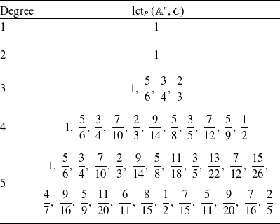
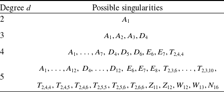
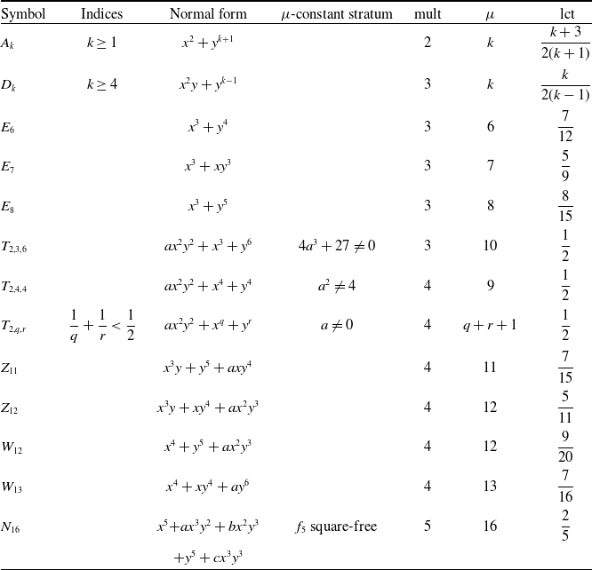

 Open access