





1. Introduction
In the early twentieth century, Lotka and Volterra pioneered the mathematical study of population dynamics, introducing models that remain central to theoretical ecology. Their work provided a foundational framework for describing predator–prey interactions and inspired a wide range of generalizations. A commonly studied form of the generalized Lotka-Volterra model is
 \begin{equation} \begin{cases} \dfrac {dx(t)}{dt}= x\alpha (x)- p(x)y, \\[12pt] \dfrac {dy(t)}{dt}=cp(x)y-dy, \end{cases} \end{equation}
where $x(t)$
and
$x(t)$
and $y(t)$
denote the prey and predator densities at time
$y(t)$
denote the prey and predator densities at time $t$
, respectively. Here,
$t$
, respectively. Here, $\alpha (x)$
describes the per capita prey growth rate in the absence of predation,
$\alpha (x)$
describes the per capita prey growth rate in the absence of predation, $c$
is the conversion efficiency of prey into predator biomass,
$c$
is the conversion efficiency of prey into predator biomass, $d$
is the predator mortality rate, and
$d$
is the predator mortality rate, and $p(x)$
is the functional response characterizing the predation rate as a function of prey density.
$p(x)$
is the functional response characterizing the predation rate as a function of prey density.
To capture the biological fact that prey consumption does not instantly translate into predator reproduction, a time delay $\tau$
is introduced. Specifically,
$\tau$
is introduced. Specifically, $\tau$
represents the period between prey capture and its conversion into viable predator biomass. The survival probability of predators during this interval is given by
$\tau$
represents the period between prey capture and its conversion into viable predator biomass. The survival probability of predators during this interval is given by $e^{-d\tau }$
[Reference Arino, Wang and Wolkowicz2]. Assuming logistic growth for the prey population and a Holling type II functional response, we obtain the delayed predator–prey system
$e^{-d\tau }$
[Reference Arino, Wang and Wolkowicz2]. Assuming logistic growth for the prey population and a Holling type II functional response, we obtain the delayed predator–prey system
 \begin{equation} \begin{cases} \dfrac {dx(t)}{dt}=rx(t)\!\left (1-\dfrac {x(t)}{K}\right )-\dfrac {mx(t)y(t)}{a+x(t)}, \\[12pt] \dfrac {dy(t)}{dt}=-dy(t)+e^{-d\tau }\dfrac {cmx(t-\tau )y(t-\tau )}{a+x(t-\tau )}, \end{cases} \end{equation}
where $r$
is the intrinsic prey growth rate,
$r$
is the intrinsic prey growth rate, $K$
is the environmental carrying capacity,
$K$
is the environmental carrying capacity, $a$
is the half-saturation constant, and
$a$
is the half-saturation constant, and $m$
is the predation rate. All parameters are positive. The incorporation of
$m$
is the predation rate. All parameters are positive. The incorporation of $\tau$
renders the model more realistic by reflecting the maturation time of predators and compensating for mortality during the delay.
$\tau$
renders the model more realistic by reflecting the maturation time of predators and compensating for mortality during the delay.
Such delayed predator–prey systems have been extensively studied from both biological and mathematical perspectives; see [Reference Cooke, Elderkin and Huang5–Reference Gourley and Kuang7, Reference Li, Lin and Wang11, Reference Li, Yuan, Jin and Wang15, Reference Mai, Sun and Wang18, Reference Song and Wei20, Reference Wang, Nagy, Gilg and Kuang23, Reference Xiao and Ruan26–Reference Xu, Shu, Tang and Wang28] and references therein. An alternative biological interpretation of the delay and survival term $e^{-d\tau }$
was proposed by Gourley and Kuang [Reference Gourley and Kuang7], who studied stage-structured models in which juvenile predators experience a mortality rate
$e^{-d\tau }$
was proposed by Gourley and Kuang [Reference Gourley and Kuang7], who studied stage-structured models in which juvenile predators experience a mortality rate $d_j \neq d$
during the maturation period
$d_j \neq d$
during the maturation period $\tau$
, leading to the survival factor
$\tau$
, leading to the survival factor $e^{-d_j\tau }$
. Related stage-structured models with Holling type I and II responses were analysed by Gourley and Kuang [Reference Gourley and Kuang7] and by Li, Lin, and Wang [Reference Li, Lin and Wang11] using Hopf bifurcation analysis. Cooke, Elderkin, and Huang [Reference Cooke, Elderkin and Huang5] incorporated juvenile prey mortality into similar delayed systems, while Fan and Wolkowicz [Reference Fan and Wolkowicz6] considered model (1.2) with a Holling type I response, demonstrating the existence of local Hopf bifurcations and a cascade of period-doublings leading to chaos. Diffusive extensions with predator maturation delay have also been investigated, for instance by Xu et al. [Reference Xu, Shu, Tang and Wang28] in the context of global Hopf bifurcation. More broadly, delay has been employed in predator–prey models to capture diverse biological mechanisms and to explore their rich dynamical behaviour [Reference Cooke, van den Driessche and Zou4, Reference Li, Yuan, Jin and Wang15, Reference Mai, Sun and Wang18, Reference Song and Wei20, Reference Shu, Hu, Wang and Watmough21, Reference Wang, Nagy, Gilg and Kuang23, Reference Xiao and Ruan26, Reference Xu27].
$e^{-d_j\tau }$
. Related stage-structured models with Holling type I and II responses were analysed by Gourley and Kuang [Reference Gourley and Kuang7] and by Li, Lin, and Wang [Reference Li, Lin and Wang11] using Hopf bifurcation analysis. Cooke, Elderkin, and Huang [Reference Cooke, Elderkin and Huang5] incorporated juvenile prey mortality into similar delayed systems, while Fan and Wolkowicz [Reference Fan and Wolkowicz6] considered model (1.2) with a Holling type I response, demonstrating the existence of local Hopf bifurcations and a cascade of period-doublings leading to chaos. Diffusive extensions with predator maturation delay have also been investigated, for instance by Xu et al. [Reference Xu, Shu, Tang and Wang28] in the context of global Hopf bifurcation. More broadly, delay has been employed in predator–prey models to capture diverse biological mechanisms and to explore their rich dynamical behaviour [Reference Cooke, van den Driessche and Zou4, Reference Li, Yuan, Jin and Wang15, Reference Mai, Sun and Wang18, Reference Song and Wei20, Reference Shu, Hu, Wang and Watmough21, Reference Wang, Nagy, Gilg and Kuang23, Reference Xiao and Ruan26, Reference Xu27].
It is well known that the corresponding ordinary differential equation (ODE) model obtained by setting $\tau =0$
in (1.2) admits a unique globally asymptotically stable periodic orbit. The focus of this paper is to uncover the richer dynamics that emerge for
$\tau =0$
in (1.2) admits a unique globally asymptotically stable periodic orbit. The focus of this paper is to uncover the richer dynamics that emerge for $\tau \gt 0$
, with particular emphasis on the global structure of Hopf bifurcation. Our main results are as follows:
$\tau \gt 0$
, with particular emphasis on the global structure of Hopf bifurcation. Our main results are as follows:
-
• There exists a sequence of local Hopf bifurcations as $\tau$
(or
$K$
) varies. Under suitable conditions, the connected components of the global Hopf bifurcation are nested with respect to
$\tau$
.
$\tau$
(or
$K$
) varies. Under suitable conditions, the connected components of the global Hopf bifurcation are nested with respect to
$\tau$
. -
• The limit cycle of the ODE model belongs to a connected component of the global Hopf bifurcation of the DDE model (1.2) in Fuller’s space. This connection between ODE periodic orbits and DDE Hopf components appears to be new.
-
• Introducing a positive delay
$\tau$
can lead to predator–prey coexistence through oscillatory dynamics at lower carrying capacities compared to the delay-free case, a counterintuitive phenomenon given the mortality losses incurred during the delay.


The novelty of the second result lies in establishing a precise relationship between ODE limit cycles and global Hopf components in delay differential equations, which to the best of our knowledge has not been reported in the context of Holling-type functional responses. The third result offers new biological insight by demonstrating that delay can in fact facilitate coexistence under more restrictive environmental conditions.
The paper is organized as follows. In Section 2, we establish the well-posedness of (1.2) with prescribed initial data and recall the known dynamics of the corresponding ODE model. Section 3 analyses local dynamics near equilibria and the onset of Hopf bifurcations. Section 4 develops the theory of global Hopf bifurcation and connected components. In Section 5, we present bifurcation diagrams in the $(\tau ,K)$
-plane, highlighting the joint effects of delay and carrying capacity. Section 6 concludes with biological interpretation and significance of the results.
$(\tau ,K)$
-plane, highlighting the joint effects of delay and carrying capacity. Section 6 concludes with biological interpretation and significance of the results.
2. Preliminaries
2.1. Existence, uniqueness, and boundedness of solutions
Let $\mathbf{C}=C([-\tau ,0],\mathbb{R}_+)$
be a set of continuous functions mapping
$\mathbf{C}=C([-\tau ,0],\mathbb{R}_+)$
be a set of continuous functions mapping $[-\tau ,0]$
to
$[-\tau ,0]$
to $\mathbb{R}_+$
equipped with the supremum norm, where
$\mathbb{R}_+$
equipped with the supremum norm, where $\mathbb{R}_+$
is the set of positive real numbers. Consider the initial data
$\mathbb{R}_+$
is the set of positive real numbers. Consider the initial data $\phi =(\phi _1(t),\phi _2(t))\in \mathbf{C\times C}$
for system (1.2). The right-hand side of system (1.2) is continuously differentiable with respect to the arguments
$\phi =(\phi _1(t),\phi _2(t))\in \mathbf{C\times C}$
for system (1.2). The right-hand side of system (1.2) is continuously differentiable with respect to the arguments $x(t)$
,
$x(t)$
, $y(t)$
,
$y(t)$
, $x(t-\tau )$
, and
$x(t-\tau )$
, and $y(t-\tau )$
. By the existence and uniqueness theorem [Reference Hale and Lunel8, Reference Kuang14], there exists a unique solution
$y(t-\tau )$
. By the existence and uniqueness theorem [Reference Hale and Lunel8, Reference Kuang14], there exists a unique solution $(x_1(t), x_2(t))$
for
$(x_1(t), x_2(t))$
for $t$
in a small neighbourhood of
$t$
in a small neighbourhood of $t=0$
and satisfies the initial condition
$t=0$
and satisfies the initial condition $(x_1(t), x_2(t))=(\phi _1(t),\phi _2(t))$
for
$(x_1(t), x_2(t))=(\phi _1(t),\phi _2(t))$
for $t\in [-\tau , 0]$
. Moreover, the solution is continuously differentiable.
$t\in [-\tau , 0]$
. Moreover, the solution is continuously differentiable.
Lemma 2.1. $x(t)$
and
$x(t)$
and $y(t)$
are positive for
$y(t)$
are positive for $t\gt 0$
given the initial condition
$t\gt 0$
given the initial condition $\phi \in \mathbf{C\times C}$
.
$\phi \in \mathbf{C\times C}$
.
Proof. It follows from the first equation of system (1.2) and the formula of variation of constants that
 \begin{equation*}x(t)=x(0)e^{ \int _{0}^{t} r(1-\frac {x(s)}{K})-\frac {my(s)}{a+x(s)}\,ds }.\end{equation*}
Since $x(0)\gt 0$
, then
$x(0)\gt 0$
, then $x(t)\gt 0$
for
$x(t)\gt 0$
for $t\gt 0$
on the interval of existence. For
$t\gt 0$
on the interval of existence. For $y(t)$
, since
$y(t)$
, since $y(0)\gt 0$
and
$y(0)\gt 0$
and $y(t)$
is continuous, then either
$y(t)$
is continuous, then either $y(t)\gt 0$
for
$y(t)\gt 0$
for $t\gt 0$
on the interval of existence, or
$t\gt 0$
on the interval of existence, or $\exists$ $t_0\gt 0,$
such that
$t_0\gt 0,$
such that $y(t_0)=0$
, but
$y(t_0)=0$
, but $y'(t_0)\leq 0$
. However, by substituting
$y'(t_0)\leq 0$
. However, by substituting $t=t_0$
into the second equation of system (1.2), we obtain
$t=t_0$
into the second equation of system (1.2), we obtain
 \begin{equation*} y'(t_0)=e^{-d\tau }\frac {cmx(t_0-\tau )y(t_0-\tau )}{a+x(t_0-\tau )}\gt 0, \end{equation*}
Which is a contradiction. Hence, $y(t)$
is positive for
$y(t)$
is positive for $t\gt 0$
.
$t\gt 0$
.
Lemma 2.2.
The solution $(x(t), y(t))$
is eventually uniformly bounded from above provided that the initial condition
$(x(t), y(t))$
is eventually uniformly bounded from above provided that the initial condition $\phi \in \mathbf{C\times C}$
.
$\phi \in \mathbf{C\times C}$
.
Proof. We will first show that $x(t)$
is eventually uniformly bounded from above. From the first equation of system (1.2), by Lemma 2.1, we have
$x(t)$
is eventually uniformly bounded from above. From the first equation of system (1.2), by Lemma 2.1, we have
 \begin{equation*}\frac {dx}{dt}=rx(t)\left(1-\frac {x(t)}{K}\right)-\frac {mx(t)y(t)}{a+x(t)}\lt rx(t)\left(1-\frac {x(t)}{K}\right).\end{equation*}
Let $X(t)$
be the solution to
$X(t)$
be the solution to $\frac {dX}{dt}=X(t)(1-\frac {X(t)}{K})$
with
$\frac {dX}{dt}=X(t)(1-\frac {X(t)}{K})$
with $X(0)=x(0)\gt 0$
. By the comparison theorem,
$X(0)=x(0)\gt 0$
. By the comparison theorem,
 \begin{equation*}\limsup _{t\rightarrow \infty }x(t)\leq \limsup _{t\rightarrow \infty }X(t)=K.\end{equation*}
To show $y(t)$
is eventually uniformly bounded from above, let
$y(t)$
is eventually uniformly bounded from above, let $U(t)=ce^{-d\tau }x(t-\tau )+y(t)$
, then
$U(t)=ce^{-d\tau }x(t-\tau )+y(t)$
, then
 \begin{eqnarray*} \frac {dU}{dt}&=&ce^{-d\tau }\frac {d(x(t-\tau ))}{dt}+\frac {d(y(t))}{dt}\\ &=&ce^{-d\tau }\left ((r+d)x(t-\tau )-\frac {r(x(t-\tau ))^2}{K}\right )-dU(t). \end{eqnarray*}
Notice that
 \begin{equation*}(r+d)x(t-\tau ) -\frac {r(x(t-\tau ))^2}{K}-\frac {(r+d)^2K}{4r}=-\left (\frac {\sqrt {r}x(t-\tau )}{\sqrt {K}}-\frac {(r+d)\sqrt {K}}{2\sqrt {r}}\right )^2\leq 0,\end{equation*}
and accordingly,
 \begin{equation*}\frac {dU}{dt}\leq ce^{-d\tau }\frac {(r+d)^2K}{4r}-dU(t).\end{equation*}
Let $Y(t)$
be the solution to
$Y(t)$
be the solution to $\frac {dY}{dt}=ce^{-d\tau }\frac {(r+d)^2K}{4r}-dY(t)$
with
$\frac {dY}{dt}=ce^{-d\tau }\frac {(r+d)^2K}{4r}-dY(t)$
with $Y(0)=U(0)$
. Then,
$Y(0)=U(0)$
. Then,
 \begin{equation*}Y(t)=\frac {ce^{-d\tau }(r+d)^2K}{4rd}+\left (U(0)-\frac {ce^{-d\tau }(r+d)^2K}{4rd}\right )e^{-dt}.\end{equation*}
By the comparison theorem,
 \begin{equation*}\limsup _{t\rightarrow \infty }y(t)\leq \limsup _{t\rightarrow \infty }U(t)\leq \limsup _{t\rightarrow \infty }Y(t)=\frac {ce^{-d\tau }(r+d)^2K}{4rd}\leq cK.\end{equation*}
Hence, $y(t)$
is eventually uniformly bounded from above.
$y(t)$
is eventually uniformly bounded from above.
Theorem 2.3.
The solution $(x(t), y(t))$
of system (1.2) exists on
$(x(t), y(t))$
of system (1.2) exists on $[-\tau , \infty )$
for
$[-\tau , \infty )$
for $\phi \in \mathbf{C\times C}$
.
$\phi \in \mathbf{C\times C}$
.
Proof. By Lemmas 2.1 and 2.2, the solution $(x(t), y(t))$
is eventually uniformly bounded. By the Continuation Theorem [Reference Hale and Lunel8, Reference Kuang14], the solution exists for all
$(x(t), y(t))$
is eventually uniformly bounded. By the Continuation Theorem [Reference Hale and Lunel8, Reference Kuang14], the solution exists for all $t\gt 0$
.
$t\gt 0$
.
2.2. Dynamics of the classical model and equilibrium points of system (1.2)
To fully understand the dynamics of the delayed model (1.2), we recall the dynamics of the classical model below, i.e., the corresponding ODE system of model (1.2), which was studied by Jing and Chen in the 1980s [Reference Jing and Chen13].
 \begin{equation} \begin{cases} \displaystyle \frac {dx(t)}{dt}=rx\left(1-\frac {x}{K}\right)-\frac {mxy}{a+x},\\[12pt] \displaystyle \frac {dy(t)}{dt}=y\left(-d+\frac {cmx}{a+x}\right). \end{cases} \end{equation}
Lemma 2.4.
Let $K_c=\frac {ad}{cm-d}$
, and
$K_c=\frac {ad}{cm-d}$
, and $K_0=\frac {a(cm+d)}{cm-d}$
. System (2.1) has three equilibrium points
$K_0=\frac {a(cm+d)}{cm-d}$
. System (2.1) has three equilibrium points $E_0(0,0)$
,
$E_0(0,0)$
, $E_K(K,0)$
and
$E_K(K,0)$
and $E^*(\frac {ad}{cm-d}, \frac {rca(Kcm-Kd-ad)}{K(cm-d)^2})$
, where
$E^*(\frac {ad}{cm-d}, \frac {rca(Kcm-Kd-ad)}{K(cm-d)^2})$
, where $E_0$
is always a saddle.
$E_0$
is always a saddle.
-
•
$E_K$
is globally asymptotically stable for
$K\lt K_c$
and becomes unstable for
$K\gt K_c$
. As
$K$
increases and crosses the threshold
$K=K_c$
, a transcritical bifurcation takes place between
$E_K$
and
$E^\ast$
.
$E_K$
loses stability and
$E^\ast$
enters the first quadrant.
-
•
$K=K_0$
is the Hopf bifurcation threshold for
$E^*$
.
$E^\ast$
is globally asymptotically stable for
$K_c\lt K\lt K_0$
and unstable for
$K\gt K_0$
. -
• System (2.1) has no periodic solution for
$K\leq K_0$
, and a unique periodic solution for
$K\gt K_0$
.


For system (1.2), it is easy to see that the equilibrium points $E_0(0, 0)$
and
$E_0(0, 0)$
and $E_K(K, 0)$
exist for all
$E_K(K, 0)$
exist for all $\tau \gt 0$
. To explore the existence and stability of interior equilibrium points, we define the following parameters for convenience:
$\tau \gt 0$
. To explore the existence and stability of interior equilibrium points, we define the following parameters for convenience:
 \begin{equation*}K_1=\frac {ad}{cme^{-d\tau }-d}, K_2=\frac {ad(3cm+d)}{c^2m^2-d^2}, \tau _{max}=\frac {1}{d} \ln \left (\frac {Kcm}{ad+dK}\right ).\end{equation*}
Then, $K_c\lt K_2\lt K_0$
and
$K_c\lt K_2\lt K_0$
and $K_c\lt K_1$
. We introduce the condition below.
$K_c\lt K_1$
. We introduce the condition below.
-
• Condition
$C_0\,:\, cm\gt d$
, and
$K\gt K_1$
(i.e.,
$\tau \lt \tau _{max}$
).


Through straightforward calculations, we derive the following lemma.
Lemma 2.5.
The interior equilibrium $E^*(\frac {da}{ce^{-d\tau }m-d},\frac {rce^{-d\tau }a(Kce^{-d\tau }m-Kd-da)}{K(ce^{-d\tau }m-d)^2})$
of system (1.2) exists under the condition
$E^*(\frac {da}{ce^{-d\tau }m-d},\frac {rce^{-d\tau }a(Kce^{-d\tau }m-Kd-da)}{K(ce^{-d\tau }m-d)^2})$
of system (1.2) exists under the condition $C_0$
.
$C_0$
.
Consider the stability of equilibrium points. Let $(x_0, y_0)$
be any equilibrium point of system (1.2) The characteristic matrix at
$(x_0, y_0)$
be any equilibrium point of system (1.2) The characteristic matrix at $(x_0, y_0)$
is given by
$(x_0, y_0)$
is given by
 \begin{equation*} J(x_0,y_0)=\begin{bmatrix} \bigg (r-\frac {2rx_0}{K}-\frac {may_0}{(a+x_0)^2}\bigg ) -\lambda & \quad \frac {-mx_0}{a+x_0} \\ e^{-\lambda \tau }\frac {ce^{-d\tau }may_0}{(a+x_0)^2} & \quad \bigg (-d+e^{-\lambda \tau }\frac {ce^{-d\tau }mx_0}{(a+x_0))}\bigg )-\lambda \end{bmatrix}.\end{equation*}
By substituting $x_0$
and
$x_0$
and $y_0$
with 0 in
$y_0$
with 0 in $J(x_0,y_0)$
, we obtain two simple eigenvalues of
$J(x_0,y_0)$
, we obtain two simple eigenvalues of $J(0, 0)$
:
$J(0, 0)$
: $\lambda _1=r\gt 0$
and
$\lambda _1=r\gt 0$
and $\lambda _2=-d\lt 0$
. Applying the Hartman–Grobman theorem [Reference Hartman9], we establish the following lemma.
$\lambda _2=-d\lt 0$
. Applying the Hartman–Grobman theorem [Reference Hartman9], we establish the following lemma.
Lemma 2.6.
Equilibrium $E_0$
is a saddle point for all
$E_0$
is a saddle point for all $\tau \geq 0$
.
$\tau \geq 0$
.
3. Local dynamics near equilibrium points
3.1. Local stability of
$E^*$

Substituting the coordinates of $E^*$
into
$E^*$
into $J(x_0, y_0)$
, we obtain
$J(x_0, y_0)$
, we obtain
 \begin{align*} J(E^\ast ) = \left[\begin{array}{c@{\quad}c} \frac {rd(K(ce^{-d\tau }m-d)-a(ce^{-d\tau }m+d))}{Kce^{-d\tau }m(ce^{-d\tau }m-d)} -\lambda & \frac {-d}{ce^{-d\tau }}\\[5pt] e^{-\lambda \tau }\frac {r(Kce^{-d\tau }m-Kd-da)}{Km} & -d+de^{-\lambda \tau }-\lambda \end{array}\right]. \end{align*}
The characteristic equation is derived by setting the determinant of $J(E^\ast )$
to zero, i.e.,
$J(E^\ast )$
to zero, i.e.,
 \begin{equation} P(\lambda ,\tau )\,:\!=\,\lambda ^2+[d-H(\tau )]\lambda +e^{-\lambda \tau }[-d\lambda +L(\tau )]-dH(\tau )=0, \end{equation}
where $H(\tau )$
and
$H(\tau )$
and $L(\tau )$
are defined as follows
$L(\tau )$
are defined as follows
 \begin{equation*}H(\tau )=r\bigg [\frac {de^{d\tau }}{cm}-\frac {ad}{K(ce^{-d\tau }m-d)}-\frac {ad^2e^{d\tau }}{(ce^{-d\tau }m-d)Kcm}\bigg ],\end{equation*}
 \begin{equation*}L(\tau )=dH(\tau )+A(\tau ), \ \text{and}\ \ A(\tau )=rd\left (\frac {Kce^{-d\tau }m-Kd-da}{Kmce^{-d\tau }}\right ),\end{equation*}
with $\tau \in [0, \tau _{max})$
. Under condition
$\tau \in [0, \tau _{max})$
. Under condition $C_0$
,
$C_0$
, $A(\tau )$
is strictly positive, and the functions
$A(\tau )$
is strictly positive, and the functions $H(\tau )$
,
$H(\tau )$
, $L(\tau )$
, and
$L(\tau )$
, and $A(\tau )$
are well defined and bounded. For simplicity, we will drop the
$A(\tau )$
are well defined and bounded. For simplicity, we will drop the $(\tau )$
and express
$(\tau )$
and express $H(\tau )$
,
$H(\tau )$
, $L(\tau )$
, and
$L(\tau )$
, and $A(\tau )$
as
$A(\tau )$
as $H, L$
, and
$H, L$
, and $A$
when necessary.
$A$
when necessary.
Lemma 3.1.
The sum of the multiplicity of roots of $P(\lambda , \tau )=0$
on
$P(\lambda , \tau )=0$
on $\mathbb{C}^+=\{\lambda \in \mathbb{C}\,:\, Re(\lambda )\gt 0\}$
can change only if a pair of conjugate complex roots appear on or cross the imaginary axis as
$\mathbb{C}^+=\{\lambda \in \mathbb{C}\,:\, Re(\lambda )\gt 0\}$
can change only if a pair of conjugate complex roots appear on or cross the imaginary axis as $\tau$
varies continuously on
$\tau$
varies continuously on $[0, \tau _{max})$
.
$[0, \tau _{max})$
.
Proof. To show that no eigenvalue emerges from infinity, we write $P(\lambda ,\tau )= \lambda ^2 +\eta (\lambda ,\tau )$
, where
$P(\lambda ,\tau )= \lambda ^2 +\eta (\lambda ,\tau )$
, where $\eta (\lambda ,\tau )=[d-H(\tau )]\lambda +e^{-\lambda \tau }[-d\lambda +L(\tau )]-dH(\tau )$
. Since
$\eta (\lambda ,\tau )=[d-H(\tau )]\lambda +e^{-\lambda \tau }[-d\lambda +L(\tau )]-dH(\tau )$
. Since $H(\tau )$
and
$H(\tau )$
and $L(\tau )$
are bounded on
$L(\tau )$
are bounded on $[0, \tau _{max})$
, we have
$[0, \tau _{max})$
, we have
 \begin{equation*}\limsup _{Re\lambda \gt 0, |\lambda | \to \infty }\big |\lambda ^{-2} \eta (\lambda ,\tau )\big |\leq \limsup _{Re\lambda \gt 0, |\lambda | \to \infty }\left (\frac {2d+|H(\tau )|}{|\lambda |}+\frac {|L(\tau )|+d|H(\tau )|}{|\lambda |^2}\right )=0\lt 1.\end{equation*}
Furthermore, $P(0, \tau )=A(\tau )\gt 0$
for
$P(0, \tau )=A(\tau )\gt 0$
for $\tau \in [0, \tau _{max})$
. Hence,
$\tau \in [0, \tau _{max})$
. Hence, $\lambda =0$
is not a root for
$\lambda =0$
is not a root for $\tau \in [0, \tau _{max})$
. By Theorem 1.4, Chapter 3 of [Reference Kuang14], the desired result is obtained.
$\tau \in [0, \tau _{max})$
. By Theorem 1.4, Chapter 3 of [Reference Kuang14], the desired result is obtained.
To study the stability of $E^\ast$
and the possibility of Hopf bifurcation at
$E^\ast$
and the possibility of Hopf bifurcation at $E^*$
as
$E^*$
as $\tau$
varies, by Lemma 3.1, we assume
$\tau$
varies, by Lemma 3.1, we assume $\lambda =\pm iw$
is a pair of purely imaginary roots of
$\lambda =\pm iw$
is a pair of purely imaginary roots of $P(\lambda , \tau )=0$
where
$P(\lambda , \tau )=0$
where $w\gt 0$
. This leads to
$w\gt 0$
. This leads to
 \begin{equation*}-w^2+ [d-H]iw+e^{-i\tau w}[{-}diw+L]-dH=0.\end{equation*}
Using Euler’s formula and equating the real and imaginary parts to zero, we obtain
 \begin{equation} \begin{cases} -w^2 +L\cos (\tau w)-dw\sin (\tau w)-dH=0,\\ (d-H)w -dw\cos (\tau w)-L\sin (\tau w)=0. \end{cases} \end{equation}
Solving for $\cos (\tau w)$
and
$\cos (\tau w)$
and $\sin (\tau w)$
, and using the assumption
$\sin (\tau w)$
, and using the assumption $\tau \in [0,\tau _{max})$
, we obtain
$\tau \in [0,\tau _{max})$
, we obtain
 \begin{equation} \begin{cases} \sin (\tau w)=\frac {dwL-HwL-d^2wH-dw^3}{L^2+d^2w^2},\\[5pt] \cos (\tau w)=\frac {LdH+Lw^2+(dw)^2-dHw^2}{L^2+d^2w^2}. \end{cases} \end{equation}
Both $\sin (\tau w)$
and
$\sin (\tau w)$
and $\cos (\tau w)$
are well defined, since
$\cos (\tau w)$
are well defined, since $L^2\geq 0$
and
$L^2\geq 0$
and $d^2w^2\gt 0$
. Applying
$d^2w^2\gt 0$
. Applying $\sin ^2(\tau w)+\cos ^2(\tau w)=1$
to (3.3), we obtain
$\sin ^2(\tau w)+\cos ^2(\tau w)=1$
to (3.3), we obtain
 \begin{equation} (d^2w^2+L^2)(w^4+H^2w^2+d^2H^2-L^2)=0. \end{equation}
Theorem 3.2.
Let $K\gt K_2$
, and define
$K\gt K_2$
, and define
 \begin{equation*}\bar {\tau }= \frac {1}{d}\ln \left (\frac {cm\sqrt {9a^2+4aK+4K^2}-3acm}{2\left (ad+dK\right )}\right ). \end{equation*}
The following statements hold.
-
(1)
$0\lt \bar {\tau }\lt \tau _{max}$
. -
(2)
$L(\tau )+dH(\tau )\gt 0$
if
$\tau \in [0, \bar {\tau })$
,
$L(\tau )+dH(\tau )=0$
if
$ \tau =\bar {\tau }$
, and
$L(\tau )+dH(\tau )\lt 0$
if
$\tau \in (\bar {\tau }, \tau _{max})$
. -
(3) The unique solution of the hexic equation ( 3.4 ) for
$0\leq \tau \lt \bar {\tau }$
and
$K\gt K_2$
is given by
(3.5)
\begin{equation} w(\tau )=\sqrt {\frac {\sqrt {((H(\tau ))^4 - 4d^2(H(\tau ))^2 + 4(L(\tau ))^2)}}{2} - \frac {(H(\tau ))^2}{2}}. \end{equation}








Proof. Statement (1) is obtained by direct calculation.
(2). $L(\tau )+dH(\tau )$
is continuous for
$L(\tau )+dH(\tau )$
is continuous for $\tau \in [0, \tau _{max})$
. It is easy to check that
$\tau \in [0, \tau _{max})$
. It is easy to check that $L(\tau )+dH(\tau )$
equals zero if and only if
$L(\tau )+dH(\tau )$
equals zero if and only if $\tau =\bar {\tau }$
, and
$\tau =\bar {\tau }$
, and
 \begin{equation*}L'(\bar {\tau })+dH'(\bar {\tau })=-\frac {4ard^2(K+a)(\sqrt {4K^2+4Ka+9a^2}-3a)}{(2K+5a-\sqrt {4K^2+4Ka+9a^2})^2K}\lt 0.\end{equation*}
Hence, the sign of $L(\tau )+dH(\tau )$
is obtained for
$L(\tau )+dH(\tau )$
is obtained for $\tau \in [0, \tau _{max})$
.
$\tau \in [0, \tau _{max})$
.
(3) Let $Z=w^2$
, and substitute
$Z=w^2$
, and substitute $Z$
into the hexic equation (3.4). Then, three solutions appear
$Z$
into the hexic equation (3.4). Then, three solutions appear
 \begin{equation*} Z_{\pm }=\frac {\pm \sqrt {H^4 - 4d^2H^2 + 4L^2}}{2}-\frac {H^2}{2}, Z_3=\frac {-L^2}{d^2}.\end{equation*}
Since $Z=w^2\gt 0$
,
$Z=w^2\gt 0$
, $Z_{-}$
and
$Z_{-}$
and $Z_3$
are discarded. To ensure
$Z_3$
are discarded. To ensure $w=\sqrt {Z_+}$
is well defined, it suffices to show
$w=\sqrt {Z_+}$
is well defined, it suffices to show
 \begin{equation*}(H(\tau ))^4 - 4d^2(H(\tau ))^2 + 4(L(\tau ))^2\gt (H(\tau ))^4,\end{equation*}
i.e., $(L(\tau ))^2\gt d^2(H(\tau ))^2$
. Since
$(L(\tau ))^2\gt d^2(H(\tau ))^2$
. Since $A(\tau )$
is positive for
$A(\tau )$
is positive for $\tau \in [0, \tau _{max})$
, we have
$\tau \in [0, \tau _{max})$
, we have $L(\tau )=dH(\tau )+A(\tau )\gt dH(\tau )$
. Moreover, by statement (2), we have
$L(\tau )=dH(\tau )+A(\tau )\gt dH(\tau )$
. Moreover, by statement (2), we have $L(\tau )\gt -dH(\tau )$
for
$L(\tau )\gt -dH(\tau )$
for $\tau \in [0, \bar {\tau })$
. In conclusion,
$\tau \in [0, \bar {\tau })$
. In conclusion, $L(\tau )\gt |dH(\tau )|$
, and
$L(\tau )\gt |dH(\tau )|$
, and $(L(\tau ))^2\gt d^2(H(\tau ))^2$
.
$(L(\tau ))^2\gt d^2(H(\tau ))^2$
.
Corollary 3.3.
The equilibrium $E^\ast$
is locally asymptotically stable if
$E^\ast$
is locally asymptotically stable if $K\leq K_2$
and
$K\leq K_2$
and $\tau \in (0, \tau _{max})$
, or
$\tau \in (0, \tau _{max})$
, or $K_2\lt K\lt K_0$
and
$K_2\lt K\lt K_0$
and $\tau \in [\bar {\tau }, \tau _{max})$
.
$\tau \in [\bar {\tau }, \tau _{max})$
.



3.2. Local Hopf bifurcation at
$E^*$

By statement (3) of Theorem3.2, we assume $0\leq \tau \leq \bar {\tau }\lt \tau _{max}$
and
$0\leq \tau \leq \bar {\tau }\lt \tau _{max}$
and $K\gt K_2$
, which guarantees that the hexic equation (3.4) has a positive root
$K\gt K_2$
, which guarantees that the hexic equation (3.4) has a positive root $w=w(\tau )$
, a necessary condition for Hopf bifurcation.
$w=w(\tau )$
, a necessary condition for Hopf bifurcation.
We explore the critical values for $\tau \in [0, \bar {\tau })$
at which Hopf bifurcation occurs. From the second equation of system (3.3), it is reasonable to define the angle
$\tau \in [0, \bar {\tau })$
at which Hopf bifurcation occurs. From the second equation of system (3.3), it is reasonable to define the angle $\tau w(\tau )$
using the inverse cosine function, while also considering the sign of
$\tau w(\tau )$
using the inverse cosine function, while also considering the sign of $\sin (\tau w(\tau ))$
. Here
$\sin (\tau w(\tau ))$
. Here $\sin (\tau w(\tau ))$
is the composition of the functions
$\sin (\tau w(\tau ))$
is the composition of the functions $\sin (\tau w)$
and
$\sin (\tau w)$
and $w(\tau )$
, which are given by the first equation of system (3.3) and equation (3.5), respectively.
$w(\tau )$
, which are given by the first equation of system (3.3) and equation (3.5), respectively.
Lemma 3.4.
Define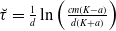 $\breve {\tau }={\frac {1}{d}\ln \left ( {\frac {cm \left ( K-a \right ) }{d \left (K+a \right ) }} \right ) }$
.
$\breve {\tau }={\frac {1}{d}\ln \left ( {\frac {cm \left ( K-a \right ) }{d \left (K+a \right ) }} \right ) }$
.
-
(1) If
$K\lt K_0$
, then
$\breve {\tau }\lt 0$
, or
$\breve {\tau }$
does not exist, and
$\sin (\tau w(\tau ))\gt 0$
for all
$\tau \in [0,\bar {\tau })$
. -
(2) If
$K=K_0$
, then
$\breve {\tau }=0$
,
$\sin (\breve {\tau } w(\breve {\tau }))= 0$
. Moreover,
$\sin (\tau w(\tau ))\gt 0$
for all
$\tau \in (0,\bar {\tau })$
. -
(3) If
$K\gt K_0$
,
$\breve {\tau }$
is well defined with
$0\lt \breve {\tau }\lt \bar {\tau }$
. Then,
$\sin (\tau w(\tau ))$
changes sign as follows:
$\sin (\tau w(\tau ))\lt 0$
for
$0\lt \tau \lt \breve {\tau }$
;
$\sin (\tau w(\tau ))=0$
for
$\tau =\breve {\tau }$
;
$\sin (\tau w(\tau ))\gt 0$
for
$\breve {\tau }\lt \tau \lt \bar {\tau }$
.















Consequently, the function $\theta _n(\tau ), \tau \in [0, \bar {\tau })$
is well defined as follows.
$\theta _n(\tau ), \tau \in [0, \bar {\tau })$
is well defined as follows.
-
• If
$\sin (\tau w(\tau ))\lt 0$
:
$\theta _n(\tau )=-\arccos \left (\frac {LdH+Lw^2+d^2w^2-dHw^2}{L^2+d^2w^2}\right )+2n\pi .$
-
• If
$\sin (\tau w(\tau ))\geq 0$
:
$\theta _n(\tau )=\arccos \left (\frac {LdH+Lw^2+d^2w^2-dHw^2}{L^2+d^2w^2}\right )+2n\pi .$




Here, $n\in \mathbb{N}$
, and
$n\in \mathbb{N}$
, and $\mathbb{N}$
is the set of all nonnegative integers.
$\mathbb{N}$
is the set of all nonnegative integers.
Proof. Solving $\sin (\tau w(\tau ))=0$
for
$\sin (\tau w(\tau ))=0$
for $H(\tau )$
, we obtain three solutions
$H(\tau )$
, we obtain three solutions
 \begin{equation*}H(\tau )=0, H(\tau )=\frac {L(\tau )}{d}, H(\tau )=2d.\end{equation*}
The solution $H(\tau )=\frac {L(\tau )}{d}$
is discarded since it is valid only for
$H(\tau )=\frac {L(\tau )}{d}$
is discarded since it is valid only for $\tau =\tau _{max}$
. The third solution
$\tau =\tau _{max}$
. The third solution $H(\tau )=2d$
is also discarded. Indeed, substituting
$H(\tau )=2d$
is also discarded. Indeed, substituting $H(\tau )=2d$
into
$H(\tau )=2d$
into $\sin (\tau w(\tau ))=0$
yields
$\sin (\tau w(\tau ))=0$
yields $|L(\tau )|+L(\tau )=0$
. Since
$|L(\tau )|+L(\tau )=0$
. Since $A(\tau )\gt 0$
, we have
$A(\tau )\gt 0$
, we have
 \begin{equation*}0\lt 2d^2+A(\tau )=dH(\tau )+A(\tau )=L(\tau )=-|L(\tau )|\leq 0,\end{equation*}
which leads to a contradiction. Therefore, the remaining solution $H(\tau )=0$
holds when
$H(\tau )=0$
holds when $\tau =\breve {\tau }$
.
$\tau =\breve {\tau }$
.
Case (1). If $K\lt K_0$
, then
$K\lt K_0$
, then $\breve {\tau }\lt 0$
, or
$\breve {\tau }\lt 0$
, or $\breve {\tau }$
does not exist. Then,
$\breve {\tau }$
does not exist. Then, $H(\tau )\lt 0$
for all
$H(\tau )\lt 0$
for all $\tau \in [0, \bar {\tau })$
. By continuity,
$\tau \in [0, \bar {\tau })$
. By continuity, $\sin (\tau w(\tau ))$
does not change sign as
$\sin (\tau w(\tau ))$
does not change sign as $\tau$
varies in
$\tau$
varies in $[0,\bar {\tau })$
. We are now investigating the sign of
$[0,\bar {\tau })$
. We are now investigating the sign of $\sin (\tau w(\tau ))$
.
$\sin (\tau w(\tau ))$
.
Since $L(\tau )=dH(\tau )+A(\tau )$
and
$L(\tau )=dH(\tau )+A(\tau )$
and $w(\tau )$
is given by (3.5), we obtain
$w(\tau )$
is given by (3.5), we obtain
 \begin{equation*} \textrm {sign}\{\sin (\tau w(\tau )\}= \textrm {sign}\{dL(\tau )-H(\tau )L(\tau )-d^2H(\tau )-d(w(\tau ))^2\}= \textrm {sign}\{\xi _1-\xi _2\}, \end{equation*}
where $\xi _1=2dA(\tau )-d(H(\tau ))^2-2A(\tau )H(\tau )$
and
$\xi _1=2dA(\tau )-d(H(\tau ))^2-2A(\tau )H(\tau )$
and $ \xi _2=d\sqrt {(H(\tau ))^4+8dA(\tau )H(\tau )+4(A(\tau ))^2}.$
Since $ L(\tau )\gt -dH(\tau )$
for
$ L(\tau )\gt -dH(\tau )$
for $\tau \in [0, \bar {\tau })$
, it follows that
$\tau \in [0, \bar {\tau })$
, it follows that $A(\tau )=L(\tau )-dH(\tau )\gt -2dH(\tau )$
. Noting that
$A(\tau )=L(\tau )-dH(\tau )\gt -2dH(\tau )$
. Noting that $H(\tau )\lt 0$
, we get
$H(\tau )\lt 0$
, we get $\xi _1\gt 3d(H(\tau ))^2-4d^2H(\tau )=dH(\tau )(3H(\tau )-4d)\gt 0$
. It is apparent that
$\xi _1\gt 3d(H(\tau ))^2-4d^2H(\tau )=dH(\tau )(3H(\tau )-4d)\gt 0$
. It is apparent that $\xi _2\geq 0$
.
$\xi _2\geq 0$
.
Next, we analyse the sign of $\xi _1^2-\xi _2^2$
. Since
$\xi _1^2-\xi _2^2$
. Since $H(\tau )\lt 0$
, we obtain
$H(\tau )\lt 0$
, we obtain
 \begin{eqnarray*} \textrm {sign}\{\xi _1^2-\xi _2^2\}&=&\textrm {sign}\{ A(\tau ) H(\tau ) \left (H(\tau ) -2 d \right ) \left (dH(\tau )+A(\tau )+d^{2}\right )\}\\ &=&\textrm {sign}\{dH(\tau )+A(\tau )+d^{2}\}\gt 0. \end{eqnarray*}
Since $A(\tau )\gt -2dH(\tau )$
, it follows that
$A(\tau )\gt -2dH(\tau )$
, it follows that $dH(\tau )+A(\tau )+d^{2}\gt -dH(\tau )+d^2\gt 0$
. Thus,
$dH(\tau )+A(\tau )+d^{2}\gt -dH(\tau )+d^2\gt 0$
. Thus, $\xi _1^2-\xi _2^2\gt 0,$
implying
$\xi _1^2-\xi _2^2\gt 0,$
implying $\xi _1\gt \xi _2\gt 0$
. Hence,
$\xi _1\gt \xi _2\gt 0$
. Hence,
 \begin{equation*}\textrm {sign}\{\sin (\tau w(\tau )\}=\textrm {sign}\{\xi _1-\xi _2\}= \frac {\textrm {sign}\{\xi ^2_1-\xi ^2_2\}}{\textrm {sign}\{\xi _1+\xi _2\}} =1, \ \forall \tau \in [0,\bar {\tau }). \end{equation*}
Cases (2) and (3). Since $K_0\gt a$
, if
$K_0\gt a$
, if $K\geq K_0$
, then
$K\geq K_0$
, then $\breve {\tau }$
is well defined. In this case, to study the sign of
$\breve {\tau }$
is well defined. In this case, to study the sign of $\sin (\tau w(\tau ))$
, it suffices to check the sign of its derivative at
$\sin (\tau w(\tau ))$
, it suffices to check the sign of its derivative at $\breve {\tau }$
. We have
$\breve {\tau }$
. We have
 \begin{equation*}\frac {d}{d\tau }(\sin (\tau w(\tau )))\big |_{\tau =\breve {\tau }}=\frac {\sqrt {\frac {a r d}{K}}\, \left (a -K \right )^{2}}{2 a^{2}}\gt 0,\end{equation*}
and which implies that $\sin (\tau w(\tau ))$
changes sign from negative to positive at
$\sin (\tau w(\tau ))$
changes sign from negative to positive at $\breve {\tau }$
. The additional condition
$\breve {\tau }$
. The additional condition $K\gt K_0$
ensures that
$K\gt K_0$
ensures that $\breve {\tau }$
is positive, and the desired results follow.
$\breve {\tau }$
is positive, and the desired results follow.
By Theorem3.2 and Lemma 3.4, we obtain two functions
 \begin{equation*}\theta =\tau w(\tau ), \ \theta =\theta _n(\tau ), \tau \in [0, \bar {\tau }].\end{equation*}
See Figure 1. These two functions are defined at $\tau =\bar {\tau }$
by continuous extension. The following lemma is obvious.
$\tau =\bar {\tau }$
by continuous extension. The following lemma is obvious.
Intersection of $\tau w(\tau )$
and
$\tau w(\tau )$
and $\theta _n(\tau )$
. Here, the graphs of
$\theta _n(\tau )$
. Here, the graphs of $\tau w(\tau )$
and>
$\tau w(\tau )$
and> $\theta _n(\tau )$
are sketched in a relatively simple way, but ensuring that the properties of Lemma 3.5 are all satisfied.
$\theta _n(\tau )$
are sketched in a relatively simple way, but ensuring that the properties of Lemma 3.5 are all satisfied.

Lemma 3.5.
Consider two functions $\theta =\tau w(\tau )$
and
$\theta =\tau w(\tau )$
and $\theta =\theta _n(\tau )$
, where
$\theta =\theta _n(\tau )$
, where $n\in \mathbb{N}$
.
$n\in \mathbb{N}$
.
-
(1)
$\theta =\tau w(\tau )\geq 0$
on
$\tau \in [0, \bar {\tau }]$
and vanishes only at
$\tau =0$
and
$\tau =\bar {\tau }$
. -
(2)
$\theta _0(0)\gt 0 (=0, \lt 0, resp.)$
if
$K\lt K_0 (=K_0, \gt K_0, resp)$
. -
(3)
$\theta _0(\bar {\tau })=\pi$
regardless of
$K$
. -
(4) If
$K\lt K_0$
, then there exists
$\zeta \gt 0$
such that
$0\lt \zeta \leq \theta _0(\tau )\leq \pi$
for
$\tau \in [0,\bar {\tau }]$
.








Proof. Statements (1) and (2) follow from Theorem3.2 and Lemma 3.4.
For statements (3) and (4), a straightforward calculation gives $\sin (\bar {\tau } w(\bar {\tau }))=0$
and
$\sin (\bar {\tau } w(\bar {\tau }))=0$
and $\cos (\bar {\tau } w(\bar {\tau }))=-1$
, which implies that
$\cos (\bar {\tau } w(\bar {\tau }))=-1$
, which implies that $\theta _0(\bar {\tau })=\pi$
. Since
$\theta _0(\bar {\tau })=\pi$
. Since $\theta _0(\tau )$
is continuous on
$\theta _0(\tau )$
is continuous on $[0, \bar {\tau }]$
, it attains the maximum and minimum values on
$[0, \bar {\tau }]$
, it attains the maximum and minimum values on $[0, \bar {\tau }]$
. By statement (1) of Lemma 3.4,
$[0, \bar {\tau }]$
. By statement (1) of Lemma 3.4, $\sin (\tau w(\tau ))\gt 0$
for all
$\sin (\tau w(\tau ))\gt 0$
for all $\tau \in [0,\bar {\tau })$
, so
$\tau \in [0,\bar {\tau })$
, so $\zeta =\displaystyle \min _{\tau \in [0,\bar {\tau }]}\theta _0(\tau )\gt 0$
and
$\zeta =\displaystyle \min _{\tau \in [0,\bar {\tau }]}\theta _0(\tau )\gt 0$
and $\displaystyle \max _{\tau \in [0,\bar {\tau }]} \theta _0(\tau )=\pi$
.
$\displaystyle \max _{\tau \in [0,\bar {\tau }]} \theta _0(\tau )=\pi$
.
Theorem 3.6.
Assume that there exists $\tau ^\star \in (0, \bar {\tau })$
such that
$\tau ^\star \in (0, \bar {\tau })$
such that
 \begin{equation*}\tau w(\tau )_{|\tau ^\star }=\theta _n(\tau )_{|\tau ^\star }, \ \text{and}\ \ (\tau w(\tau ))'_{|\tau ^\star }\neq (\theta _n(\tau ))'_{|\tau ^\star }\end{equation*}
for some $n\in \mathbb{N}$
. Then system (1.2) undergoes a Hopf bifurcation at
$n\in \mathbb{N}$
. Then system (1.2) undergoes a Hopf bifurcation at $\tau =\tau ^\star$
, and a family of non-constant periodic solutions exists in a neighbourhood of
$\tau =\tau ^\star$
, and a family of non-constant periodic solutions exists in a neighbourhood of $E^\ast$
for
$E^\ast$
for $\tau$
in a small neighbourhood of
$\tau$
in a small neighbourhood of $\tau =\tau ^\star$
.
$\tau =\tau ^\star$
.
Proof. Let $\lambda (\tau )=\alpha (\tau )\pm i\beta (\tau )$
be a pair of conjugate complex eigenvalues of
$\lambda (\tau )=\alpha (\tau )\pm i\beta (\tau )$
be a pair of conjugate complex eigenvalues of $P(\lambda , \tau )=0$
. The condition
$P(\lambda , \tau )=0$
. The condition $\tau w(\tau )_{|\tau ^\star }=\theta _n(\tau )_{|\tau ^\star }$
implies that
$\tau w(\tau )_{|\tau ^\star }=\theta _n(\tau )_{|\tau ^\star }$
implies that $\alpha (\tau ^\star )=0$
and
$\alpha (\tau ^\star )=0$
and $\beta (\tau ^\star )=w(\tau ^\star )\gt 0$
, meaning that
$\beta (\tau ^\star )=w(\tau ^\star )\gt 0$
, meaning that $P(\lambda , \tau )=0$
has a pair of purely imaginary eigenvalues
$P(\lambda , \tau )=0$
has a pair of purely imaginary eigenvalues $\pm iw(\tau ^\star )$
at
$\pm iw(\tau ^\star )$
at $\tau =\tau ^\star$
. Next, we check the transversality condition by defining the function
$\tau =\tau ^\star$
. Next, we check the transversality condition by defining the function
 \begin{equation*}S_n(\tau )=\tau -\frac {\theta _n(\tau )}{w(\tau )}, n\in \mathbb{N}.\end{equation*}
By Theorem 2.2 of [Reference Beretta and Kuang3] (the geometric stability switch criterion), we obtain
 \begin{equation*} \delta (\tau ^\star )\,:\!=\,\textrm {sign} \bigg \{\frac {d \alpha (\tau )}{d\tau }\bigg |_{\tau =\tau ^\star } \bigg \}=\textrm {sign} \bigg \{\frac {d F(w(\tau ))}{dw}\bigg |_{\tau =\tau ^\star } \bigg \}\cdot \textrm {sign}\bigg \{\frac {d S_n(\tau )}{d\tau }\bigg |_{\tau =\tau ^\star } \bigg \}, \end{equation*}
where $F(w(t))=(w(\tau ))^4+(H(\tau ))^2(w(\tau ))^2+d^2(H(\tau ))^2-(L(\tau ))^2$
. Thus,
$F(w(t))=(w(\tau ))^4+(H(\tau ))^2(w(\tau ))^2+d^2(H(\tau ))^2-(L(\tau ))^2$
. Thus,
 \begin{equation*}F_w(w(\tau ))=4(w(\tau ))^3+2(H(\tau ))^2w(\tau )\gt 0, \, \forall \tau \in (0,\bar {\tau }).\end{equation*}
By the definition of $S_n(\tau )$
, we have
$S_n(\tau )$
, we have
 \begin{equation*} \frac {dS_n(\tau )}{d\tau }=1-\frac {\theta '_n(\tau )w(\tau )-w'(\tau )\theta _n(\tau )}{(w(\tau ))^2}=\frac {\tau (w(\tau ))^2-[\theta _n'(\tau )\tau w(\tau )- \tau w'(\tau )\theta _n(\tau )]}{\tau (w(\tau ))^2}.\end{equation*}
Since $(\tau w(\tau ))'=\tau w'(\tau ) +w(\tau )$
, we get
$(\tau w(\tau ))'=\tau w'(\tau ) +w(\tau )$
, we get $\tau w'(\tau )=(\tau w(\tau ))'-w(\tau )$
. Noting that
$\tau w'(\tau )=(\tau w(\tau ))'-w(\tau )$
. Noting that $ \theta _n(\tau ^\star )=\tau ^\star w(\tau ^\star )$
, we obtain
$ \theta _n(\tau ^\star )=\tau ^\star w(\tau ^\star )$
, we obtain
 \begin{eqnarray*} \frac {dS_n(\tau )}{d\tau }\bigg |_{\tau =\tau ^\star }&=&\dfrac {\tau ^\star (w(\tau ^\star ))^2-\theta _n'(\tau ^\star )\tau ^\star w(\tau ^\star )+\big[(\tau w(\tau ))'_{|\tau ^\star }-w(\tau ^\star )\big]\tau ^\star w(\tau ^\star )}{\tau ^\star (w(\tau ^\star ))^2}\\ &=&\dfrac {\tau ^\star w(\tau ^\star )\big[(\tau w(\tau ))'_{|\tau ^\star }-\theta _n'(\tau ^\star )\big]}{\tau ^\star (w(\tau ^\star ))^2}=\dfrac {(\tau w(\tau ))'_{|\tau ^\star }-\theta _n'(\tau ^\star )}{w(\tau ^\star )}. \end{eqnarray*}
Since $w(\tau ^\star )\gt 0$
, we obtain
$w(\tau ^\star )\gt 0$
, we obtain
 \begin{equation*}\delta (\tau ^\star )=\textrm {sign}\{ (\tau w)'-\theta '_n(\tau )_{|\tau =\tau ^\star }\}\neq 0,\end{equation*}
which completes the proof.
Remark 3.7. $\delta (\tau ^\star )$
reveals the direction along which the complex conjugate eigenvalues
$\delta (\tau ^\star )$
reveals the direction along which the complex conjugate eigenvalues $\lambda =\alpha (\tau )\pm i\beta (\tau )$
cross the imaginary axis as
$\lambda =\alpha (\tau )\pm i\beta (\tau )$
cross the imaginary axis as $\tau$
increases through
$\tau$
increases through $\tau =\tau ^\star$
. If
$\tau =\tau ^\star$
. If $\delta (\tau ^\star )=1$
(resp.
$\delta (\tau ^\star )=1$
(resp. $\delta (\tau ^\star )=-1$
),
$\delta (\tau ^\star )=-1$
), $\lambda$
crosses the imaginary axis from left to right (resp. from right to left). If
$\lambda$
crosses the imaginary axis from left to right (resp. from right to left). If $\delta (\tau ^\star )\neq 0$
, the graphs of two functions
$\delta (\tau ^\star )\neq 0$
, the graphs of two functions $\theta =\tau w(\tau )$
and
$\theta =\tau w(\tau )$
and $\theta =\theta _n(\tau )$
intersect transversely at
$\theta =\theta _n(\tau )$
intersect transversely at $\tau =\tau ^\star$
. Otherwise, the two graphs are tangent.
$\tau =\tau ^\star$
. Otherwise, the two graphs are tangent.
It is technically challenging to characterize the number of intersections between $\theta =\tau w(\tau )$
and
$\theta =\tau w(\tau )$
and $\theta =\theta _n(\tau )$
or the roots of
$\theta =\theta _n(\tau )$
or the roots of $S_n(\tau )=0$
,
$S_n(\tau )=0$
, $n\in \mathbb{N}$
. There may be no roots or several roots.
$n\in \mathbb{N}$
. There may be no roots or several roots.
Definition 3.8.
Let $\chi (n)$
be the number of roots of
$\chi (n)$
be the number of roots of $S_n(\tau )=0$
on
$S_n(\tau )=0$
on $(0, \bar {\tau })$
, where
$(0, \bar {\tau })$
, where $n\in \mathbb{N}$
.
$n\in \mathbb{N}$
.
The following hypothesis is necessary for the occurrence of Hopf bifurcation.
-
(H1) Suppose that
$S_n(\tau )=0$
has finitely many roots on
$(0, \bar {\tau })$
, i.e.,
$0\leq \chi (n)\lt \infty , \forall n\in \mathbb{N}$
, and these
$\chi (n)$
roots are given and arranged in the following orderwith
\begin{equation*}\tau _n^{(1)}\lt \tau _n^{(2)}\lt \cdots \lt \tau _n^{(i)}\lt \cdots \tau _n^{(\chi (n))},\end{equation*}
$\delta (\tau _n^{(i)})=\pm 1$
$(i=1, 2, \cdots , \chi (n))$
.






Remark 3.9.
Let $\Lambda =\{j\in \mathbb{N}|\chi (j)\neq 0\}$
. If
$\Lambda =\{j\in \mathbb{N}|\chi (j)\neq 0\}$
. If $\chi (n)=2$
for all
$\chi (n)=2$
for all $n\in \Lambda$
, then we denote
$n\in \Lambda$
, then we denote $\tau _n^{(1)}$
and
$\tau _n^{(1)}$
and $\tau _n^{(2)}$
as
$\tau _n^{(2)}$
as $\tau _n^{-}$
and
$\tau _n^{-}$
and $\tau _n^{+}$
, respectively.
$\tau _n^{+}$
, respectively.
Example 1.
Two sets of parameters are chosen to show the distribution of roots of $S_n(\tau )=0$
.
$S_n(\tau )=0$
.
-
(a) Choose
$K= 1, r=30, m =1, c=4, d=0.1, a=1$
. See Figure 2(a). Here,
$K\lt K_0=\frac {41}{39}$
, and we have
$\chi (0)=\chi (1)=\chi (2)=\chi (3)=2$
, and
$\chi (n)=0$
for
$n\geq 4$
. The critical Hopf bifurcation values are
\begin{align*} \left .\begin{array}{llll} \tau _0^-=0.013562, & \tau _0^+=23.67336, & \tau _1^-=3.8062, & \tau _1^+=21.49988,\\ \tau _2^-=7.81234, & \tau _2^+=19.55209, & \tau _3^-=12.7067, & \tau _3^+=17.10348. \end{array}\right . \end{align*}
-
(b) Choose
$K= 20, r=10, m =1, c=4, d=0.1, a=5$
. See Figure 2(b). Here,
$K\gt K_0=\frac {205}{39}$
, and we have
$\chi (0)=1$
,
$\chi (1)=2$
,
$\chi (2)=4$
, and
$\chi (n)=0$
for
$n\geq 3$
. The critical Hopf bifurcation values are
\begin{align*} \left .\begin{array}{llll} \tau _0^{(1)}=32.42808, & \tau _1^{(1)}=6.2049, & \tau _1^{(2)}=32.22374, & \\ \tau _2^{(1)}=13.96008, & \tau _2^{(2)}=24.85518, & \tau _2^{(3)}=30.21286, & \tau _2^{(4)}=32.00694. \end{array}\right . \end{align*}








Corollary 3.10.
Assume (H1), then Hopf bifurcation occurs at a sequence of critical values $\tau =\tau _n^{(i)}$
and there exists a family of non-constant periodic solutions in a neighbourhood of
$\tau =\tau _n^{(i)}$
and there exists a family of non-constant periodic solutions in a neighbourhood of $E^\ast$
for
$E^\ast$
for $\tau$
in a small neighbourhood of
$\tau$
in a small neighbourhood of $\tau =\tau _n^{(i)}$
.
$\tau =\tau _n^{(i)}$
.
The following is an attempt to study the roots of $S_n(\tau )=0$
for certain special cases.
$S_n(\tau )=0$
for certain special cases.
Proposition 3.11.
Let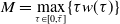 $M=\displaystyle \max _{\tau \in [0, \bar {\tau }]}\{\tau w(\tau )\}$
. Assume that
$M=\displaystyle \max _{\tau \in [0, \bar {\tau }]}\{\tau w(\tau )\}$
. Assume that
 \begin{equation*}K\lt K_0, \ \text{and}\ \ (2N+1)\pi \lt M\lt (2N+3)\pi \end{equation*}
for some $N \in \mathbb{N}$
. Then, there are three cases.
$N \in \mathbb{N}$
. Then, there are three cases.
-
(1) If
$n\leq N$
,
$\theta _n(\tau )$
intersects
$\tau w(\tau )$
at least twice.
-
(2) If
$n=N+1$
,
$\theta _n(\tau )$
and
$\tau w(\tau )$
intersect either at least twice, or once tangentially, or they never intersect.
-
(3) If
$n\geq N+2$
,
$\theta _n(\tau )$
and
$\tau w(\tau )$
never intersect in
$(0,\bar {\tau })$
.


Proof. By Lemma 3.5, $\theta _n(\tau )$
ranges between
$\theta _n(\tau )$
ranges between $[\zeta +2n\pi , (2n+1)\pi ]$
. From statement (1) of Lemma 3.5, we have
$[\zeta +2n\pi , (2n+1)\pi ]$
. From statement (1) of Lemma 3.5, we have $\tau w(\tau )\big |_{\tau =0}=0$
and
$\tau w(\tau )\big |_{\tau =0}=0$
and $ \tau w(\tau )\big |_{\tau =\bar {\tau }}=0$
and
$ \tau w(\tau )\big |_{\tau =\bar {\tau }}=0$
and $M\gt 0$
. For the first case, from the intermediate value theorem, it follows that
$M\gt 0$
. For the first case, from the intermediate value theorem, it follows that $\theta _n(\tau )$
must intersect
$\theta _n(\tau )$
must intersect $\tau w(\tau )$
at least twice since
$\tau w(\tau )$
at least twice since $\theta _n(0)\geq \zeta +2n\pi \gt 0$
,
$\theta _n(0)\geq \zeta +2n\pi \gt 0$
, $M\gt (2N+1)\pi \gt \max _{\tau \in [0, \bar {\tau }]}\theta _n(\tau )$
, and
$M\gt (2N+1)\pi \gt \max _{\tau \in [0, \bar {\tau }]}\theta _n(\tau )$
, and $\theta _n(\bar {\tau })\gt 0$
. For the third case, we have
$\theta _n(\bar {\tau })\gt 0$
. For the third case, we have $n\geq N+2$
, hence
$n\geq N+2$
, hence $\min _{\tau \in [0, \bar {\tau }]}\theta _n(\tau )\gt 2n\pi \geq 2(N+2)\pi \gt M$
and the result follows. The second case is trivial, as all possibilities might hold here.
$\min _{\tau \in [0, \bar {\tau }]}\theta _n(\tau )\gt 2n\pi \geq 2(N+2)\pi \gt M$
and the result follows. The second case is trivial, as all possibilities might hold here.
3.3. Local dynamics and bifurcations involving
$E_K$

Theorem 3.12.
-
(1)
$E_K$
is asymptotically stable for
$\tau \gt \tau _{max}$
and unstable for
$0\lt \tau \lt \tau _{max}$
. -
(2) System (1.2) undergoes a transcritical bifurcation involving
$E_K$
and
$E^\ast$
at
$\tau =\tau _{max}.$


Proof. (1) The characteristics equation at $E_K$
has the following form
$E_K$
has the following form
 \begin{equation*} (\lambda +r)\left(\lambda +d-\frac {ce^{-d\tau }mK}{a+K}e^{-\lambda \tau }\right)=0. \end{equation*}
Therefore, $\lambda =-r$
is an eigenvalue, and the other eigenvalues are the roots of the equation
$\lambda =-r$
is an eigenvalue, and the other eigenvalues are the roots of the equation
 \begin{equation} Q(\lambda )\,:\!=\,\lambda +d-\frac {ce^{-d\tau }mK}{a+K}e^{-\lambda \tau }=0. \end{equation}
As one did for $E^\ast$
, an analogous analysis can be performed to investigate the stability of
$E^\ast$
, an analogous analysis can be performed to investigate the stability of $E_K$
. Here, using Theorem4.7(a) in Chapter 4 of [Reference Smith22] we conclude that
$E_K$
. Here, using Theorem4.7(a) in Chapter 4 of [Reference Smith22] we conclude that $E_K$
is asymptotically stable if
$E_K$
is asymptotically stable if $\tau \gt \tau _{max}$
. If
$\tau \gt \tau _{max}$
. If $0\lt \tau \lt \tau _{max}$
, then
$0\lt \tau \lt \tau _{max}$
, then $Q(0)\lt 0$
. Note that
$Q(0)\lt 0$
. Note that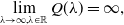 $\displaystyle \lim _{\lambda \rightarrow \infty , \lambda \in \mathbb{R}}Q(\lambda )=\infty ,$
by continuity of
$\displaystyle \lim _{\lambda \rightarrow \infty , \lambda \in \mathbb{R}}Q(\lambda )=\infty ,$
by continuity of $Q(\lambda )$
, there exists a positive real root. Hence,
$Q(\lambda )$
, there exists a positive real root. Hence, $E_K$
is always unstable.
$E_K$
is always unstable.
(2) If $\tau =\tau _{max}$
, then
$\tau =\tau _{max}$
, then $E_K=E^\ast$
and
$E_K=E^\ast$
and $Q(0)=0, Q'(0)=1+d\tau _{max}\neq 0$
. Hence,
$Q(0)=0, Q'(0)=1+d\tau _{max}\neq 0$
. Hence, $\lambda =0$
is a simple eigenvalue.
$\lambda =0$
is a simple eigenvalue.
Let $\hat {\lambda }(\tau )$
be a root of
$\hat {\lambda }(\tau )$
be a root of $Q(\lambda )=0$
such that
$Q(\lambda )=0$
such that $\hat {\lambda }(\tau _{max})=0$
. To verify that
$\hat {\lambda }(\tau _{max})=0$
. To verify that $E_K$
changes stability at
$E_K$
changes stability at $\tau = \tau _{max}$
, we compute
$\tau = \tau _{max}$
, we compute
 \begin{equation*}\frac {d}{d\tau }\textrm {Re}(\hat {\lambda })\bigg |_{\tau =\tau _{max}}=-\frac { cmdKe^{-d\tau }}{a+K+\tau cmK e^{-d\tau }}\bigg |_{\tau =\tau _{max}} \lt 0.\end{equation*}
As a consequence, $E_K$
changes stability from unstable to stable. To investigate the stability switch of
$E_K$
changes stability from unstable to stable. To investigate the stability switch of $E^*$
at
$E^*$
at $\tau =\tau _{max}$
, let
$\tau =\tau _{max}$
, let $\tilde {\lambda }(\tau )$
be a root of
$\tilde {\lambda }(\tau )$
be a root of $P(\lambda , \tau )=0$
such that
$P(\lambda , \tau )=0$
such that $\tilde {\lambda }(\tau _{max})=0$
. By the chain rule, we have
$\tilde {\lambda }(\tau _{max})=0$
. By the chain rule, we have
 \begin{equation*} \frac {dP(\lambda ,\tau )}{d\tau } = \frac {\partial P(\lambda ,\tau )}{\partial \lambda }\frac {d\lambda }{d\tau } + \frac {\partial P(\lambda ,\tau )}{\partial \tau } =0. \end{equation*}
Substituting $\tau =\tau _{\max }$
and using
$\tau =\tau _{\max }$
and using $\tilde {\lambda }(\tau _{\max })=0$
, we obtain
$\tilde {\lambda }(\tau _{\max })=0$
, we obtain
 \begin{equation*} \left .\frac {dP(\lambda , \tau )}{d\tau }\right |_{\tau =\tau _{\max }} = -dH'(\tau )+L'(\tau ) - \frac {d\tilde {\lambda }}{d\tau }\bigl (H(\tau )+\tau L(\tau )\bigr ) \Big |_{\tau =\tau _{\max }}. \end{equation*}
Solving for $\frac {d\tilde {\lambda }}{d\tau }$
and taking the real part yields
$\frac {d\tilde {\lambda }}{d\tau }$
and taking the real part yields
 \begin{equation*}\textrm {Re}\left (\frac {d}{d\tau }\tilde {\lambda }\right )\bigg |_{\tau =\tau _{max}}=\frac {d}{d\tau }\textrm {Re}(\tilde {\lambda })\bigg |_{\tau =\tau _{max}}=\frac {L'(\tau )-dH'(\tau )}{H(\tau )+\tau L(\tau )}\bigg |_{\tau =\tau _{max}}=\frac {d^2}{\ln \left (\frac {cmK}{d\,\left (a+K\right )}\right )+1}\gt 0. \end{equation*}
Hence, the real part of $\tilde {\lambda }$
changes sign at
$\tilde {\lambda }$
changes sign at $\tau =\tau _{max}$
from negative to positive. This implies that
$\tau =\tau _{max}$
from negative to positive. This implies that $E^*$
moves from the first quadrant to the fourth quadrant and changes stability from stable to unstable. Thus,
$E^*$
moves from the first quadrant to the fourth quadrant and changes stability from stable to unstable. Thus, $E_K$
and
$E_K$
and $E^\ast$
exchange stability at
$E^\ast$
exchange stability at $\tau =\tau _{max}$
, where they merge in a transcritical bifurcation.
$\tau =\tau _{max}$
, where they merge in a transcritical bifurcation.
4. Global Hopf bifurcation and continuity of branches
By the local Hopf bifurcation Theorem3.6 and Corollary 3.10, the periodic solutions bifurcating from $E^\ast$
exist in a small neighbourhood of a sequence of critical values
$E^\ast$
exist in a small neighbourhood of a sequence of critical values $\tau =\tau _n^{(i)}$
where
$\tau =\tau _n^{(i)}$
where $i=1, 2, \cdots , \chi (n)$
and
$i=1, 2, \cdots , \chi (n)$
and $n\in \mathbb{N}$
. In this section, we study the evolution of periodic solutions as
$n\in \mathbb{N}$
. In this section, we study the evolution of periodic solutions as $\tau$
varies within
$\tau$
varies within $(0, \tau _{max})$
. The global Hopf bifurcation theory developed by Wu is implemented (see Theorem 3.3 of [Reference Wu25]), and connected components of non-trivial periodic solutions in Fuller’s space are considered. By estimating the period of the period solution and studying the
$(0, \tau _{max})$
. The global Hopf bifurcation theory developed by Wu is implemented (see Theorem 3.3 of [Reference Wu25]), and connected components of non-trivial periodic solutions in Fuller’s space are considered. By estimating the period of the period solution and studying the $\tau$
-interval in which the period solution exists, we can describe the onset and termination of Hopf bifurcation branches under certain conditions.
$\tau$
-interval in which the period solution exists, we can describe the onset and termination of Hopf bifurcation branches under certain conditions.
Let $\tilde {x}(t)=x(t\tau )$
,
$\tilde {x}(t)=x(t\tau )$
, $\tilde {y}(t)=y(t\tau )$
, then system (1.2) can be rewritten as
$\tilde {y}(t)=y(t\tau )$
, then system (1.2) can be rewritten as
 \begin{equation} \dot {z}=F(z_t,\tau ,T), \ (t, \tau , T)\in \mathbb{R}_+\times (0, \tau _{max})\times \mathbb{R}_+, \end{equation}
where
 \begin{equation*}z(t)=\begin{bmatrix} \tilde {x}(t)\\ \tilde {y}(t) \end{bmatrix}, \, F(z_t,\tau ,T)= \begin{bmatrix} \tau r\tilde {x}(t)\left(1-\frac {\tilde {x}(t)}{K}\right)-\tau \frac {m\tilde {x}(t)\tilde {y}(t)}{a+\tilde {x}(t)}\\[5pt] -\tau d \tilde {y}(t)+\tau e^{-d\tau }\frac {cm\tilde {x}(t-1)\tilde {y}(t-1)}{a+\tilde {x}(t-1)} \end{bmatrix}. \end{equation*}
Let $z_t(s)=z(t+s)$
for
$z_t(s)=z(t+s)$
for $s\in [-1,0]$
, so that
$s\in [-1,0]$
, so that $z_t\in C([-1, 0], \mathbb{R}^2_+)$
. Hence, the domain of
$z_t\in C([-1, 0], \mathbb{R}^2_+)$
. Hence, the domain of $F(z_t,\tau , T)$
is
$F(z_t,\tau , T)$
is $ C([-1, 0], \mathbb{R}^2_+) \times (0,\tau _{max}) \times \mathbb{R}_+$
. By identifying the subspace of
$ C([-1, 0], \mathbb{R}^2_+) \times (0,\tau _{max}) \times \mathbb{R}_+$
. By identifying the subspace of $C([-1, 0], \mathbb{R}^2_+)$
consisting of all constant mapping with
$C([-1, 0], \mathbb{R}^2_+)$
consisting of all constant mapping with $\mathbb{R}^2_+$
, we obtain a restricted mapping
$\mathbb{R}^2_+$
, we obtain a restricted mapping
 \begin{equation*}\tilde {F}(z,\tau ,T)\,:\!=\,F(z_t,\tau ,T)_{|\mathbb{R}_+^2\times (0,\tau _{max})\times \mathbb{R}_+}= \begin{bmatrix} \tau r\tilde {x}\left(1-\frac {\tilde {x}}{K}\right)-\tau \frac {m\tilde {x}\tilde {y}}{a+\tilde {x}}\\[5pt] -\tau d\tilde {y}+\tau e^{-d\tau }\frac {cm\tilde {x}\tilde {y}}{a+\tilde {x}} \end{bmatrix}. \end{equation*}
Then, $\tilde {F}$
is twice continuously differentiable, and condition (A1) of Theorem 3.3 of [Reference Wu25] is fulfilled.
$\tilde {F}$
is twice continuously differentiable, and condition (A1) of Theorem 3.3 of [Reference Wu25] is fulfilled.
Let $\mathscr{N}\,(F)=\{(z,\tau ,T)| \tilde {F}(z,\tau ,T)=0\}$
be the set of stationary solutions of system (4.1). From our analysis in Section 3, we know
$\mathscr{N}\,(F)=\{(z,\tau ,T)| \tilde {F}(z,\tau ,T)=0\}$
be the set of stationary solutions of system (4.1). From our analysis in Section 3, we know
 \begin{equation*}\mathscr{N}\,(F)=\{(z, \tau , T)| z\in \{E_0, E_K, E^\ast \}, (\tau , T)\in (0, \tau _{max})\times \mathbb{R}_+\}.\end{equation*}
It is apparent that the function $F(z_t, \tau , T)$
is continuously differentiable with respect to its first argument
$F(z_t, \tau , T)$
is continuously differentiable with respect to its first argument $z_t$
and the characteristics matrix function at the stationary solution
$z_t$
and the characteristics matrix function at the stationary solution $(z, \tau , T)\in \mathscr{N}\,(F)$
is
$(z, \tau , T)\in \mathscr{N}\,(F)$
is
 \begin{equation*}\Delta _{(z,\tau ,T)}(\lambda )=\lambda Id-DF(z, \tau , T)(e^{\lambda \cdot } Id).\end{equation*}
Here, $DF(z, \tau , T)$
is the complexification of the derivative of
$DF(z, \tau , T)$
is the complexification of the derivative of $F(z_t, \tau , T)$
with respect to
$F(z_t, \tau , T)$
with respect to $z_t$
evaluated at
$z_t$
evaluated at $(z, \tau , T)\in \mathscr{N}\,(F)$
. Since
$(z, \tau , T)\in \mathscr{N}\,(F)$
. Since $\Delta _{(z,\tau ,T)}$
is continuous, condition (A3) of Theorem 3.3 of [Reference Wu25] is fulfilled.
$\Delta _{(z,\tau ,T)}$
is continuous, condition (A3) of Theorem 3.3 of [Reference Wu25] is fulfilled.
Furthermore, by Lemma 2.6 and Theorem3.12, we establish that $\lambda =0$
is not an eigenvalue of
$\lambda =0$
is not an eigenvalue of $E_0$
,
$E_0$
, $E_K$
, or
$E_K$
, or $E^\ast$
for
$E^\ast$
for $\tau \in (0, \tau _{max})$
, meaning
$\tau \in (0, \tau _{max})$
, meaning $\text{det}(DF(z, \tau , T))\neq 0$
for
$\text{det}(DF(z, \tau , T))\neq 0$
for $(z, \tau , T)\in \mathscr{N}\,(F)$
. Thus,
$(z, \tau , T)\in \mathscr{N}\,(F)$
. Thus, $DF(z, \tau , T)$
is isomorphic to
$DF(z, \tau , T)$
is isomorphic to $\mathbb{R}^2$
at each stationary solution, and condition (A2) of Theorem 3.3 of [Reference Wu25] is fulfilled.
$\mathbb{R}^2$
at each stationary solution, and condition (A2) of Theorem 3.3 of [Reference Wu25] is fulfilled.
For the global Hopf bifurcation, by Lemma 2.1 and Theorem3.6, $(E^*, \tau , T)\in \mathscr{N}\,(F)$
is the only stationary solution under consideration. Assume condition (H1) is satisfied, i.e.,
$(E^*, \tau , T)\in \mathscr{N}\,(F)$
is the only stationary solution under consideration. Assume condition (H1) is satisfied, i.e., $S_n(\tau )=0$
has
$S_n(\tau )=0$
has $\chi (n)$
roots on
$\chi (n)$
roots on $(0, \bar {\tau })$
, where
$(0, \bar {\tau })$
, where $\chi (n)\lt \infty , \forall n\in \mathbb{N}$
, and these
$\chi (n)\lt \infty , \forall n\in \mathbb{N}$
, and these $\chi (n)$
roots are given and arranged in the following order
$\chi (n)$
roots are given and arranged in the following order
 \begin{equation*}\tau _n^{(1)}\lt \tau _n^{(2)}\lt \cdots \lt \tau _n^{(i)}\lt \cdots \tau _n^{(\chi (n))}.\end{equation*}
Furthermore, $\delta (\tau _n^{(i)})=\pm 1$ $(i=1, 2, \cdots , \chi (n))$
.
$(i=1, 2, \cdots , \chi (n))$
.
By the definition of a centre for a stationary solution [Reference Wu25], the points
 \begin{equation} \left(E^\ast , \tau _n^{(i)}, \frac {2\pi }{\tau _n^{(i)}w(\tau _n^{(i)})}\right)=\left(E^\ast , \tau _n^{(i)}, \frac {2\pi }{\theta _n(\tau _n^{(i)})}\right), \ n\in \mathbb{N}, \ i=1, 2,\cdots , \chi (n) \end{equation}
are centres of system (4.1). For each centre, it is the only centre in its small neighbourhood, and it only has finitely many purely imaginary characteristic values, whose imaginary part takes the form
 \begin{equation*}\tau _n^{(i)}w\left(\tau _n^{(i)}=i\frac {2\pi }{2\pi /(\tau _n^{(i)}w(\tau _n^{(i)}))}=\frac {2\pi }{2\pi /(\theta _n(\tau _n^{(i)}))}.\right.\end{equation*}
Here, $T_n^{(i)}\,:\!=\,2\pi /(\tau _n^{(i)}w(\tau _n^{(i)}))=2\pi /(\theta _n(\tau _n^{(i)}))$
is the minimal period of periodic solution bifurcating at
$T_n^{(i)}\,:\!=\,2\pi /(\tau _n^{(i)}w(\tau _n^{(i)}))=2\pi /(\theta _n(\tau _n^{(i)}))$
is the minimal period of periodic solution bifurcating at $\tau _n^{(i)}$
for the scaled model (4.1). Therefore,
$\tau _n^{(i)}$
for the scaled model (4.1). Therefore, $(E^*,\tau _n^{(i)}, \frac {2\pi }{\theta (\tau _n^{(i)})})$
given in (4.2) are isolated centres. Moreover, the first crossing number of each isolated centre
$(E^*,\tau _n^{(i)}, \frac {2\pi }{\theta (\tau _n^{(i)})})$
given in (4.2) are isolated centres. Moreover, the first crossing number of each isolated centre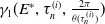 $\gamma _1(E^*,\tau _n^{(i)}, \frac {2\pi }{\theta (\tau _n^{(i)})})$
is well defined, and
$\gamma _1(E^*,\tau _n^{(i)}, \frac {2\pi }{\theta (\tau _n^{(i)})})$
is well defined, and
 \begin{equation*}\gamma _1\left(E^*,\tau _n^{(i)}, \frac {2\pi }{\theta (\tau _n^{(i)})}\right)=-\textrm {sign}\left (\frac {d}{d\tau }Re(\lambda )\big |_{\tau =\tau _n^{(i)}}\right )=-\textrm {sign}(S'(\tau _n^{(i)}))=-\delta (\tau _n^{(i)})=\pm 1.\end{equation*}
Hence, condition (A4) of Theorem 3.3 of [Reference Wu25] is fulfilled.
Define the closed set $\Sigma (F)$
in
$\Sigma (F)$
in $C([-1, 0], \mathbb{R}^2_+)\times (0, \tau _{max})\times \mathbb{R}_+$
as follows:
$C([-1, 0], \mathbb{R}^2_+)\times (0, \tau _{max})\times \mathbb{R}_+$
as follows:
 \begin{equation*}\Sigma (F)=Cl\{(z,\tau ,T) \in C([-1, 0], \mathbb{R}^2_+)\times (0, \tau _{max})\times \mathbb{R}_+|z\ \text{is a $T$-periodic solution of system (4.1)}\}.\end{equation*}
Let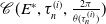 $\mathscr{C}\,(E^*,\tau _n^{(i)}, \frac {2\pi }{\theta (\tau _n^{(i)})})$
be the connected component of
$\mathscr{C}\,(E^*,\tau _n^{(i)}, \frac {2\pi }{\theta (\tau _n^{(i)})})$
be the connected component of $(E^*,\tau _n^{(i)}, \frac {2\pi }{\theta (\tau _n^{(i)})})$
in
$(E^*,\tau _n^{(i)}, \frac {2\pi }{\theta (\tau _n^{(i)})})$
in $\Sigma (F).$
By ensuring that conditions (A1)-(A4) of Theorem 3.3 in [Reference Wu25] hold, we can now apply the global Hopf bifurcation theorem to system (4.1).
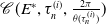
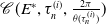
Theorem 4.1. Consider the system (4.1) with (H1). One of the following two statements holds.
-
(i)
$\mathscr{C}\,(E^*,\tau _n^{(i)}, \frac {2\pi }{\theta (\tau _n^{(i)})})$
is unbounded;
-
(ii)
$\mathscr{C}\,(E^*,\tau _n^{(i)}, \frac {2\pi }{\theta (\tau _n^{(i)})})$
is bounded, the intersection
$\mathscr{C}\,(E^*,\tau _n^{(i)}, \frac {2\pi }{\theta (\tau _n^{(i)})}) \cap \mathscr{N}\,(F)$
is finite, and
\begin{equation*}\sum _{(z,\tau ,T)\in \mathscr{C}\,\left(E^*,\tau _n^{(i)}, \frac {2\pi }{\theta (\tau _n^{(i)})}\right)\cap \mathscr{N}\,(F)}\gamma _1(z,\tau ,T)=0.\end{equation*}


Here, $i=1, 2,\cdots , \chi (n)$
and
$i=1, 2,\cdots , \chi (n)$
and $n\in \mathbb{N}$
.
$n\in \mathbb{N}$
.
In the following, we analyse the boundedness and connections of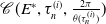 $\mathscr{C}\,(E^*,\tau _n^{(i)}, \frac {2\pi }{\theta (\tau _n^{(i)})})$
.
$\mathscr{C}\,(E^*,\tau _n^{(i)}, \frac {2\pi }{\theta (\tau _n^{(i)})})$
.
Lemma 4.2.
Let $\Gamma \,:\!=\,\{(\xi _1(t), \xi _2(t))\,:\, t\in [0, \infty )\}$
be any non-constant periodic solution of system (1.2) with initial condition
$\Gamma \,:\!=\,\{(\xi _1(t), \xi _2(t))\,:\, t\in [0, \infty )\}$
be any non-constant periodic solution of system (1.2) with initial condition $\phi \in \mathbf{C\times C}$
. Then
$\phi \in \mathbf{C\times C}$
. Then $0\lt \xi _1(t)\leq K, 0\lt \xi _2(t)\leq cK,$
for all
$0\lt \xi _1(t)\leq K, 0\lt \xi _2(t)\leq cK,$
for all $t\geq 0$
.
$t\geq 0$
.
Proof. By Lemma 2.1, $\xi _1$
and
$\xi _1$
and $\xi _2$
are positive for all
$\xi _2$
are positive for all $t\geq 0$
. By Lemma 2.2, we have
$t\geq 0$
. By Lemma 2.2, we have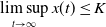 $\displaystyle \limsup _{t\rightarrow \infty } x(t)\leq K$
. We assert that
$\displaystyle \limsup _{t\rightarrow \infty } x(t)\leq K$
. We assert that $\xi _1(t)\leq K$
for all
$\xi _1(t)\leq K$
for all $t\geq 0$
. If not, then there exists
$t\geq 0$
. If not, then there exists $t_1\gt 0$
such that
$t_1\gt 0$
such that $\xi _1(t_1)\gt K$
. Then,
$\xi _1(t_1)\gt K$
. Then,
 \begin{equation*}K\lt \xi _1(t_1)=\lim _{n\rightarrow \infty }\xi _1(t_1+nT)\leq \limsup _{t\rightarrow \infty } \xi _1(t)\leq K,\end{equation*}
which is a contradiction. By a similar argument, we conclude that $\xi _2(t)\leq cK$
for all
$\xi _2(t)\leq cK$
for all $t\geq 0$
.
$t\geq 0$
.
Lemma 4.3.
If $K\lt K_0$
, system (4.1) has no periodic solutions of period 1.
$K\lt K_0$
, system (4.1) has no periodic solutions of period 1.
Proof. At a periodic solution with period 1, we have $\tilde {x}(t-1)=\tilde {x}(t)$
and
$\tilde {x}(t-1)=\tilde {x}(t)$
and $\tilde {y}(t-1)=\tilde {y}(t)$
. To show that system (4.1) has no periodic solution of period 1, we replace
$\tilde {y}(t-1)=\tilde {y}(t)$
. To show that system (4.1) has no periodic solution of period 1, we replace $\tilde {x}(t-1)$
and
$\tilde {x}(t-1)$
and $\tilde {y}(t-1)$
with
$\tilde {y}(t-1)$
with $\tilde {x}(t)$
and
$\tilde {x}(t)$
and $\tilde {y}(t)$
, respectively, reducing system (4.1) to the ODE system
$\tilde {y}(t)$
, respectively, reducing system (4.1) to the ODE system
 \begin{equation} \begin{cases} \frac {d\tilde {x}}{dt}=\tau r\tilde {x}\left(1-\frac {\tilde {x}}{K}\right)-\tau \frac {m\tilde {x}\tilde {y}}{a+\tilde {x}},\\[5pt] \frac {d\tilde {y}}{dt}=\tau \tilde {y}\left(-d+ce^{-d\tau }\frac {m\tilde {x}}{a+\tilde {x}}\right). \end{cases} \end{equation}
By Lemma 2.4 and substituting $c$
with
$c$
with $ce^{-d\tau }$
, we obtain that system (4.3) does not have a periodic solution when
$ce^{-d\tau }$
, we obtain that system (4.3) does not have a periodic solution when $K\lt \frac {a(cme^{-d\tau }+d)}{cme^{-d\tau }-d}$
. Notice that
$K\lt \frac {a(cme^{-d\tau }+d)}{cme^{-d\tau }-d}$
. Notice that $K_0=\frac {a(cm+d)}{cm-d}\lt \frac {a(cme^{-d\tau }+d)}{cme^{-d\tau }-d}$
, and therefore system (4.3) has no periodic solutions if
$K_0=\frac {a(cm+d)}{cm-d}\lt \frac {a(cme^{-d\tau }+d)}{cme^{-d\tau }-d}$
, and therefore system (4.3) has no periodic solutions if $K\lt K_0$
. Consequently, system (4.1) has no periodic solutions of period 1.
$K\lt K_0$
. Consequently, system (4.1) has no periodic solutions of period 1.
We have the estimate of $T_n^{(i)}$
, the minimal period of periodic solution bifurcating at
$T_n^{(i)}$
, the minimal period of periodic solution bifurcating at $\tau _n^{(i)}$
for the scaled model (4.1) below.
$\tau _n^{(i)}$
for the scaled model (4.1) below.
Lemma 4.4.
If $K\lt K_0$
, then
$K\lt K_0$
, then $T_n^{(i)}\in (\frac {1}{n+1},\frac {1}{n})$
for
$T_n^{(i)}\in (\frac {1}{n+1},\frac {1}{n})$
for $i=1,2,\cdots\!, \chi (n)$
and
$i=1,2,\cdots\!, \chi (n)$
and $n=1, 2,\cdots$
.
$n=1, 2,\cdots$
.
Proof. By Lemma 3.5, we have $2n\pi +\zeta \leq \theta _n(\tau _n^{(i)})\leq (2n+1)\pi$
for all
$2n\pi +\zeta \leq \theta _n(\tau _n^{(i)})\leq (2n+1)\pi$
for all $\tau \in [0,\bar {\tau }]$
. Then
$\tau \in [0,\bar {\tau }]$
. Then
 \begin{equation*}\frac {1}{n+1}=\frac {2\pi }{(2n+2)\pi }\lt \frac {2\pi }{(2n+1)\pi }\leq T_n^{(i)}\leq \frac {2\pi }{2n\pi +\zeta }\lt \frac {1}{n}.\end{equation*}
Theorem 4.5.
For system (4.1), $E_K$
is globally asymptotically stable for
$E_K$
is globally asymptotically stable for $\tau \geq \tau _{max}$
, and periodic solutions exist only on
$\tau \geq \tau _{max}$
, and periodic solutions exist only on $(0,\tau _{max})$
.
$(0,\tau _{max})$
.
Proof. Consider the Lyapunov functional
 \begin{equation*} V(\tilde {x}, \tilde {y})=\tilde {x}-K-K\ln {\frac {\tilde {x}}{K}}+\frac {mK}{da}\tilde {y}+\tau \frac {cm^2Ke^{-d\tau }}{da}\int _{t-1}^{t}\frac {\tilde {x}(s)\tilde {y}(s)}{a+\tilde {x}(s)}ds. \end{equation*}
By Lemma 2.1, $V(\tilde {x}, \tilde {y})$
is well-defined. Furthermore,
$V(\tilde {x}, \tilde {y})$
is well-defined. Furthermore, $V(\tilde {x}, \tilde {y})\geq 0$
for all
$V(\tilde {x}, \tilde {y})\geq 0$
for all $\tilde {x}\gt 0, \tilde {y}\geq 0$
, and
$\tilde {x}\gt 0, \tilde {y}\geq 0$
, and $V(\tilde {x}, \tilde {y})=0$
if and only if
$V(\tilde {x}, \tilde {y})=0$
if and only if $(\tilde {x}, \tilde {y})=(K, 0)$
, we compute the total derivative along system (4.1) with respect to
$(\tilde {x}, \tilde {y})=(K, 0)$
, we compute the total derivative along system (4.1) with respect to $t$
:
$t$
:
 \begin{eqnarray*} \dot {V}(\tilde {x}, \tilde {y})&=&r\tau \tilde {x}(t)\left(1-\frac {\tilde {x}(t)}{K}\right)-\tau \frac {m\tilde {x}(t)\tilde {y}(t)}{a+\tilde {x}(t)}-K\tau \left (r\left(1-\frac {\tilde {x}(t)}{K}\right)-\frac {m\tilde {y}(t)}{a+\tilde {x}(t)}\right )\\ & &+\,\tau \frac {cm^2Ke^{-d\tau }}{da}\cdot \frac {\tilde {x}(t-1)\tilde {y}(t-1)}{a+\tilde {x}(t-1)}-\tau \frac {mK}{a}\tilde {y}(t)\\ & &+\,\tau \frac {cm^2Ke^{-d\tau }}{da}\cdot \frac {\tilde {x}(t)\tilde {y}(t)}{a+\tilde {x}(t)}-\tau \frac {cm^2Ke^{-d\tau }}{da}\cdot \frac {\tilde {x}(t-1)\tilde {y}(t-1)}{a+\tilde {x}(t-1)}\\ &=&\tau \left [-\frac {r}{K}(K-\tilde {x})^2 +\tilde {y}\left (\frac {-m\tilde {x}+Km}{a+\tilde {x}}-\frac {mK}{a}+\frac {cm^2Ke^{-d\tau }\tilde {x}}{da(a+\tilde {x})}\right )\right ]. \end{eqnarray*}
For $\tau \geq \tau _{max}$
, we obtain
$\tau \geq \tau _{max}$
, we obtain
 \begin{eqnarray*} \dot {V}(\tilde {x}, \tilde {y})&\leq & \tau \left [-\frac {r}{K}(K-\tilde {x})^2 +\tilde {y}\left (\frac {-m\tilde {x}+Km}{a+\tilde {x}}-\frac {mK}{a}+\frac {cm^2Ke^{-d\tau _{max}}\tilde {x}}{da(a+\tilde {x})}\right )\right ]\\ &=&-\frac {\tau r}{K}(K-\tilde {x})^2\leq 0. \end{eqnarray*}
The last equality holds if and only if $\tilde {x}=K$
and
$\tilde {x}=K$
and $\tilde {y}\geq 0$
. From the first equation of system (4.1), the largest invariant set of
$\tilde {y}\geq 0$
. From the first equation of system (4.1), the largest invariant set of $\{(K, \tilde {y})|\tilde {y}\geq 0\}$
is the singleton
$\{(K, \tilde {y})|\tilde {y}\geq 0\}$
is the singleton $\{(K, 0)\}$
. By Lyapunov–LaSalle’s invariance principle [Reference Kuang14],
$\{(K, 0)\}$
. By Lyapunov–LaSalle’s invariance principle [Reference Kuang14], $(K,0)$
is globally asymptotically stable for
$(K,0)$
is globally asymptotically stable for $\tau \geq \tau _{max}$
.
$\tau \geq \tau _{max}$
.
Theorem 4.6.
Consider system (4.1), under the assumption (H1) with $K\lt K_0$
. Then the following two statements hold.
$K\lt K_0$
. Then the following two statements hold.
-
(1) All connected components
$\mathscr{C}\,(E^*,\tau _n^{(i)}, \frac {2\pi }{\theta (\tau _n^{(i)})})$
are bounded for all
$n=1, 2, \cdots$
. -
(2) If
$\chi (n)=2$
, denote
$\tau _n^{(1)}$
and
$\tau _n^{(2)}$
as
$\tau _n^{-}$
and
$\tau _n^{+}$
, respectively. Then the connected components
$\mathscr{C}\,(E^*,\tau _n^{-}, \frac {2\pi }{\theta (\tau _n^{-})})$
and
$\mathscr{C}\,(E^*,\tau _n^{+}, \frac {2\pi }{\theta (\tau _n^{+})})$
coincide and are nested. The connected component
$\mathscr{C}\,(E^*,\tau _n^{\pm }, \frac {2\pi }{\theta (\tau _n^{\pm })})$
connects exactly two bifurcation points
$\tau _n^-$
and
$\tau _n^+$
, where
$n=1, 2, \cdots$
.
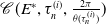


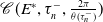
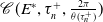
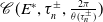


Proof. (1). By Lemma 4.2, all periodic solutions of system (4.1) are uniformly bounded. Therefore, the projection of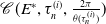 $\mathscr{C}\,(E^*,\tau _n^{(i)}, \frac {2\pi }{\theta (\tau _n^{(i)})})$
onto
$\mathscr{C}\,(E^*,\tau _n^{(i)}, \frac {2\pi }{\theta (\tau _n^{(i)})})$
onto $C([-1, 0], \mathbb{R}^2_+)$
is bounded.
$C([-1, 0], \mathbb{R}^2_+)$
is bounded.
By Lemmas 2.4 and 4.5, no periodic solution exists for $\tau =0$
or
$\tau =0$
or $\tau \geq \tau _{max}$
. Consequently, the connected components do not extend beyond the finite interval
$\tau \geq \tau _{max}$
. Consequently, the connected components do not extend beyond the finite interval $(0,\tau _{max})$
. Hence, the projection of
$(0,\tau _{max})$
. Hence, the projection of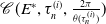 $\mathscr{C}\,(E^*,\tau _n^{(i)}, \frac {2\pi }{\theta (\tau _n^{(i)})})$
onto
$\mathscr{C}\,(E^*,\tau _n^{(i)}, \frac {2\pi }{\theta (\tau _n^{(i)})})$
onto $\tau$
-space is bounded.
$\tau$
-space is bounded.
Furthermore, by Lemma 4.3, there are no periodic solutions of period 1, and consequently, none with period $\frac {1}{n}, n=1,2,\cdots$
. By the continuity of the connected component, the projection of
$\frac {1}{n}, n=1,2,\cdots$
. By the continuity of the connected component, the projection of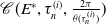 $\mathscr{C}\,(E^*,\tau _n^{(i)}, \frac {2\pi }{\theta (\tau _n^{(i)})})$
onto the
$\mathscr{C}\,(E^*,\tau _n^{(i)}, \frac {2\pi }{\theta (\tau _n^{(i)})})$
onto the $T$
-space is a subset of the finite interval
$T$
-space is a subset of the finite interval $(\frac {1}{n+1}, \frac {1}{n})$
. Hence, all connected components
$(\frac {1}{n+1}, \frac {1}{n})$
. Hence, all connected components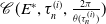 $\mathscr{C}\,(E^*,\tau _n^{(i)}, \frac {2\pi }{\theta (\tau _n^{(i)})})$
are bounded in Fuller’s space, where
$\mathscr{C}\,(E^*,\tau _n^{(i)}, \frac {2\pi }{\theta (\tau _n^{(i)})})$
are bounded in Fuller’s space, where $n=1, 2, \cdots$
.
$n=1, 2, \cdots$
.
(2). By Lemma 4.4, the minimal period of the periodic solution bifurcating at $\tau _n^{\pm }$
is
$\tau _n^{\pm }$
is $T_n^{\pm }=\frac {2\pi }{\theta (\tau _n^{\pm })}\in (\frac {1}{n+1}, \frac {1}{n})$
. By Lemma 4.3, the projection of
$T_n^{\pm }=\frac {2\pi }{\theta (\tau _n^{\pm })}\in (\frac {1}{n+1}, \frac {1}{n})$
. By Lemma 4.3, the projection of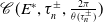 $\mathscr{C}\,(E^*,\tau _n^{\pm }, \frac {2\pi }{\theta (\tau _n^{\pm })})$
onto the
$\mathscr{C}\,(E^*,\tau _n^{\pm }, \frac {2\pi }{\theta (\tau _n^{\pm })})$
onto the $T$
-space is a subset of the finite interval
$T$
-space is a subset of the finite interval $(\frac {1}{n+1}, \frac {1}{n})$
. Moreover,
$(\frac {1}{n+1}, \frac {1}{n})$
. Moreover,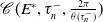 $\mathscr{C}\,(E^*,\tau _n^{-}, \frac {2\pi }{\theta (\tau _n^{-})})$
and
$\mathscr{C}\,(E^*,\tau _n^{-}, \frac {2\pi }{\theta (\tau _n^{-})})$
and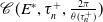 $\mathscr{C}\,(E^*,\tau _n^{+}, \frac {2\pi }{\theta (\tau _n^{+})})$
are the only two connected components whose third arguments belong to
$\mathscr{C}\,(E^*,\tau _n^{+}, \frac {2\pi }{\theta (\tau _n^{+})})$
are the only two connected components whose third arguments belong to $(\frac {1}{n+1}, \frac {1}{n})$
.
$(\frac {1}{n+1}, \frac {1}{n})$
.
By Theorem4.1, the first crossing number of $(E^*,\tau _n^{\pm }, \frac {2\pi }{\theta (\tau _n^{\pm })})$
on
$(E^*,\tau _n^{\pm }, \frac {2\pi }{\theta (\tau _n^{\pm })})$
on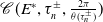 $\mathscr{C}\,(E^*,\tau _n^{\pm }, \frac {2\pi }{\theta (\tau _n^{\pm })})$
satisfies
$\mathscr{C}\,(E^*,\tau _n^{\pm }, \frac {2\pi }{\theta (\tau _n^{\pm })})$
satisfies
 \begin{equation*}\sum _{(z,\tau ,T)\in \mathscr{C}\,(E^*,\tau _n^{\pm }, \frac {2\pi }{\theta (\tau _n^{\pm })})\cap \mathscr{N}\,(F)}\gamma _1(z,\tau ,T)=0.\end{equation*}
Note that
 \begin{equation*}\gamma _1\left(E^*,\tau _n^{-}, \frac {2\pi }{\theta (\tau _n^-)}\right)=-1, \ \text{and}\ \ \gamma _1\left(E^*,\tau _n^{+}, \frac {2\pi }{\theta (\tau _n^+)}\right)=1.\end{equation*}
Hence,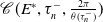 $\mathscr{C}\,(E^*,\tau _n^{-}, \frac {2\pi }{\theta (\tau _n^{-})})$
and
$\mathscr{C}\,(E^*,\tau _n^{-}, \frac {2\pi }{\theta (\tau _n^{-})})$
and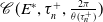 $\mathscr{C}\,(E^*,\tau _n^{+}, \frac {2\pi }{\theta (\tau _n^{+})})$
must coincide, initiating at
$\mathscr{C}\,(E^*,\tau _n^{+}, \frac {2\pi }{\theta (\tau _n^{+})})$
must coincide, initiating at $\tau =\tau _n^-$
and terminating at
$\tau =\tau _n^-$
and terminating at $\tau _n^+$
in the
$\tau _n^+$
in the $\tau$
-space (or vice versa). Since
$\tau$
-space (or vice versa). Since $\tau _j^-\lt \tau _i^-\lt \tau _i^+\lt \tau _j^+$
for
$\tau _j^-\lt \tau _i^-\lt \tau _i^+\lt \tau _j^+$
for $j\lt i$
, the components
$j\lt i$
, the components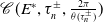 $\mathscr{C}\,(E^*,\tau _n^{\pm }, \frac {2\pi }{\theta (\tau _n^{\pm })})$
are nested, where
$\mathscr{C}\,(E^*,\tau _n^{\pm }, \frac {2\pi }{\theta (\tau _n^{\pm })})$
are nested, where $n=1, 2, \cdots$
.
$n=1, 2, \cdots$
.
If $\chi (0)=2$
and assume the projection of
$\chi (0)=2$
and assume the projection of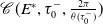 $\mathscr{C}\,(E^*,\tau _0^{-}, \frac {2\pi }{\theta (\tau _0^{-})})$
and
$\mathscr{C}\,(E^*,\tau _0^{-}, \frac {2\pi }{\theta (\tau _0^{-})})$
and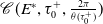 $\mathscr{C}\,(E^*,\tau _0^{+}, \frac {2\pi }{\theta (\tau _0^{+})})$
onto the
$\mathscr{C}\,(E^*,\tau _0^{+}, \frac {2\pi }{\theta (\tau _0^{+})})$
onto the $T$
-space are bounded, by Theorem4.1 and a similar argument as that of Theorem4.6, we obtain the following result.
$T$
-space are bounded, by Theorem4.1 and a similar argument as that of Theorem4.6, we obtain the following result.
Theorem 4.7.
Let $K\lt K_0$
and
$K\lt K_0$
and $\chi (0)=2$
. If the projection of
$\chi (0)=2$
. If the projection of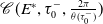 $\mathscr{C}\,(E^*,\tau _0^{-}, \frac {2\pi }{\theta (\tau _0^{-})})$
and
$\mathscr{C}\,(E^*,\tau _0^{-}, \frac {2\pi }{\theta (\tau _0^{-})})$
and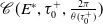 $\mathscr{C}\,(E^*,\tau _0^{+}, \frac {2\pi }{\theta (\tau _0^{+})})$
onto the
$\mathscr{C}\,(E^*,\tau _0^{+}, \frac {2\pi }{\theta (\tau _0^{+})})$
onto the $T$
-space are bounded, then they coincide and connect two bifurcation points
$T$
-space are bounded, then they coincide and connect two bifurcation points $\tau _0^-$
and
$\tau _0^-$
and $\tau _0^+$
.
$\tau _0^+$
.
Proof. By Lemma 4.2, all periodic solutions of system (4.1) are uniformly bounded. Therefore, the projection of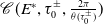 $\mathscr{C}\,(E^*,\tau _0^{\pm }, \frac {2\pi }{\theta (\tau _0^{\pm })})$
onto
$\mathscr{C}\,(E^*,\tau _0^{\pm }, \frac {2\pi }{\theta (\tau _0^{\pm })})$
onto $C([-1, 0], \mathbb{R}^2_+)$
is bounded. By Lemmas 2.4 and 4.5, no periodic solution extends beyond the interval
$C([-1, 0], \mathbb{R}^2_+)$
is bounded. By Lemmas 2.4 and 4.5, no periodic solution extends beyond the interval $(0,\tau _{\max })$
, so the projection of
$(0,\tau _{\max })$
, so the projection of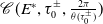 $\mathscr{C}\,(E^*,\tau _0^{\pm }, \frac {2\pi }{\theta (\tau _0^{\pm })})$
onto
$\mathscr{C}\,(E^*,\tau _0^{\pm }, \frac {2\pi }{\theta (\tau _0^{\pm })})$
onto $\tau$
-space is bounded. It follows from the assumption that
$\tau$
-space is bounded. It follows from the assumption that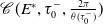 $\mathscr{C}\,(E^*,\tau _0^{-}, \frac {2\pi }{\theta (\tau _0^{-})})$
and
$\mathscr{C}\,(E^*,\tau _0^{-}, \frac {2\pi }{\theta (\tau _0^{-})})$
and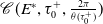 $\mathscr{C}\,(E^*,\tau _0^{+}, \frac {2\pi }{\theta (\tau _0^{+})})$
are the only two connected components whose third components lie in a bounded subset of
$\mathscr{C}\,(E^*,\tau _0^{+}, \frac {2\pi }{\theta (\tau _0^{+})})$
are the only two connected components whose third components lie in a bounded subset of $(1, \infty )$
, and the product of their first crossing numbers satisfies
$(1, \infty )$
, and the product of their first crossing numbers satisfies
 \begin{equation*} \gamma _1\left (E^*,\tau _0^{-}, \frac {2\pi }{\theta (\tau _0^{-})}\right )\cdot \gamma _1\left (E^*,\tau _0^{+}, \frac {2\pi }{\theta (\tau _0^{+})}\right ) = -1. \end{equation*}
Therefore, by Theorem4.1, the two components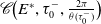 $\mathscr{C}\big(E^*,\tau _0^{-}, \frac {2\pi }{\theta (\tau _0^{-})}\big)$
and
$\mathscr{C}\big(E^*,\tau _0^{-}, \frac {2\pi }{\theta (\tau _0^{-})}\big)$
and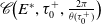 $\mathscr{C}\big(E^*,\tau _0^{+}, \frac {2\pi }{\theta (\tau _0^{+})}\big)$
coincide and connect two bifurcation points
$\mathscr{C}\big(E^*,\tau _0^{+}, \frac {2\pi }{\theta (\tau _0^{+})}\big)$
coincide and connect two bifurcation points $\tau _0^-$
and
$\tau _0^-$
and $\tau _0^+$
.
$\tau _0^+$
.
It is important to note that the nonexistence of periodic solutions in the ODE system (2.1) (i.e., system (1.2) plays a crucial role in establishing the boundedness and connectedness of the connected components, as demonstrated in the proof of Theorem4.6. However, when $K\gt K_0$
, system (1.2) admits a periodic solution at
$K\gt K_0$
, system (1.2) admits a periodic solution at $\tau =0$
. Consequently, system (4.1) also possesses a periodic solution of period 1. As a result, we lose the ability to estimate the period of the connected components in the
$\tau =0$
. Consequently, system (4.1) also possesses a periodic solution of period 1. As a result, we lose the ability to estimate the period of the connected components in the $T$
-space, and whether
$T$
-space, and whether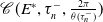 $\mathscr{C}\,(E^*,\tau _n^{-}, \frac {2\pi }{\theta (\tau _n^{-})})$
and
$\mathscr{C}\,(E^*,\tau _n^{-}, \frac {2\pi }{\theta (\tau _n^{-})})$
and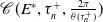 $\mathscr{C}\,(E^*,\tau _n^{+}, \frac {2\pi }{\theta (\tau _n^{+})})$
coincide remains unclear if
$\mathscr{C}\,(E^*,\tau _n^{+}, \frac {2\pi }{\theta (\tau _n^{+})})$
coincide remains unclear if $\chi (n)=2$
(see Figure 3 for these two connected components. It is not clear whether they are connected due to the computational challenge).
$\chi (n)=2$
(see Figure 3 for these two connected components. It is not clear whether they are connected due to the computational challenge).
Global Hopf bifurcation and connected components for $K\lt K_0$
. The parameters and values of
$K\lt K_0$
. The parameters and values of $\tau _n^\pm (n=0, 1, 2, 3)$
are provided in Example 1 (a).
$\tau _n^\pm (n=0, 1, 2, 3)$
are provided in Example 1 (a).

Nevertheless, we will explore the relations between the connected components for $K\gt K_0$
through numerical analysis using DDE-BifTool. Instead of analysing
$K\gt K_0$
through numerical analysis using DDE-BifTool. Instead of analysing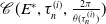 $\mathscr{C}\,(E^*,\tau _n^{(i)}, \frac {2\pi }{\theta (\tau _n^{(i)})})$
for system (4.1), we consider the connected components
$\mathscr{C}\,(E^*,\tau _n^{(i)}, \frac {2\pi }{\theta (\tau _n^{(i)})})$
for system (4.1), we consider the connected components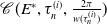 $\mathscr{C}\,(E^*,\tau _n^{(i)}, \frac {2\pi }{w(\tau _n^{(i)})})$
for system (1.2), since a periodic solution exists at
$\mathscr{C}\,(E^*,\tau _n^{(i)}, \frac {2\pi }{w(\tau _n^{(i)})})$
for system (1.2), since a periodic solution exists at $\tau =0$
.
$\tau =0$
.
-
• A unique connected component and the limit cycle of the ODE model (2.1).
If
$\chi (0)=1$
and
$\chi (n)=0$
for
$n\geq 1$
,
$S_0(\tau )=0$
has a unique root
$\tau =\tau _0^{(1)}$
on
$[0, \bar {\tau })$
and system (1.2) has a unique connected component
$\mathscr{C}\,(E^*,\tau _0^{(1)}, \frac {2\pi }{w(\tau _0^{(1)})})$
. When
$\tau =0$
,
$J(E^\ast )$
has a pair of conjugate complex eigenvalues with positive real part, meaning
$E^\ast$
is unstable and a stable limit cycle
$\Gamma _0$
(i.e, an isolated periodic solution) exists around
$E^\ast$
. As
$\tau$
increases from
$0$
to
$\tau _0^{(1)}$
, and passes by
$\tau _0^{(1)}$
, Lemma 3.1 implies that this pair of complex eigenvalues vary continuously, crossing the imaginary axis from right to left at
$\tau =\tau _0^{(1)}$
so that
$E^\ast$
becomes stable. Meanwhile, the limit cycle
$\Gamma _0$
evolves continuously. However,
$\Gamma _0$
does not necessarily persist over the entire interval
$[0, \tau _0^{(1)})$
, as it may vanish due to a bifurcation of periodic solutions at some
$\tau \lt \tau _0^{(1)}$
. If no such bifurcation occurs for
$\tau \in (0, \tau _0^{(1)})$
, then
$\Gamma _0$
must disappear through a local Hopf bifurcation at
$\tau =\tau _0^{(1)}$
, i.e.,
$(\Gamma _0, 0, \frac {2\pi }{\bar {w}})\in \mathscr{C}\,(E^*,\tau _0^{(1)}, \frac {2\pi }{w(\tau _0^{(1)})})$
, where
$\bar {w}$
is the frequency of the limit cycle
$\Gamma _0$
.Thus, the limit cycle of the ODE model (2.1) belongs to a connected component of the Hopf bifurcation of the DDE model (1.2) in Fuller’s space. As illustrated in Figure 4,
$\Gamma _0$
varies continuously on
$[0, \tau _0^{(1)}]$
and terminates
$\tau =\tau _0^{(1)}$
through a Hopf bifurcation.


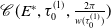





Global Hopf bifurcation and a unique connected component $\mathscr{C}\,(E^*,\tau _0^{(1)}, 2\pi /w(\tau _0^{(1)}))$
for
$\mathscr{C}\,(E^*,\tau _0^{(1)}, 2\pi /w(\tau _0^{(1)}))$
for $K\gt K_0$
. The left panel shows the amplitude and the right panel displays the period of the periodic solution for
$K\gt K_0$
. The left panel shows the amplitude and the right panel displays the period of the periodic solution for $\tau \in [0, \tau _0^{(1)}]$
. The parameter are
$\tau \in [0, \tau _0^{(1)}]$
. The parameter are $K=7, r=1, m=1, c=1, d=0.1, a=5$
, and
$K=7, r=1, m=1, c=1, d=0.1, a=5$
, and $K\gt K_0=6.11$
.
$K\gt K_0=6.11$
.

-
• Multiple connected components.
-
If
$\chi (n)\gt 2$
for some
$n\in \mathbb{N}$
, then
$S_n(\tau )=0$
has
$\chi (n)$
critical values
$\tau =\tau _n^{{(i)}}$
, leading to
$\chi (n)$
connected components
$\mathscr{C}\,(E^*,\tau _n^{(i)}, \frac {2\pi }{\theta (\tau _n^{(i)})})$
, where
$i=1, 2, \cdots , \chi (n)$
. Studying the relationship between these connected components is technically challenging, regardless of whether
$K\lt K_0$
or
$K\gt K_0$
. To illustrate this complexity, we consider the parameter values from Example1(b), where
$\chi (0)=1, \chi (1)=2$
,
$\chi (2)=4$
, and
$\chi (n)=0$
for
$n\geq 3$
. Based on Figure 5 we have the following observations:Figure 5.Global Hopf bifurcation and multiple connected components for
$K\gt K_0$
. The right panel is a magnified view of the left panel near
$\tau =\tau _0^{(1)}$
. The parameter values and
$\tau _n^{(i)} (n=0, 1, 2)$
are specified in Example 1 (b).


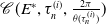






-
– For
$n=0$
:
$\mathscr{C}\,(E^*,\tau _0^{(1)}, \frac {2\pi }{w(\tau _0^{(1)})})$
initials at
$\tau _0^{(1)}$
, and experiences a sequence of saddle-node bifurcations of limit cycles occurs in the interval
$[32.33, 32.4]$
. The curve does not extend any further due to computational challenges. -
– For
$n=1$
:
$\mathscr{C}\,(E^*,\tau _1^{(1)}, \frac {2\pi }{w(\tau _1^{(1)})})$
and
$\mathscr{C}\,(E^*,\tau _1^{(2)}, \frac {2\pi }{w(\tau _1^{(2)})})$
coincide, i.e., the periodic solution initials at
$\tau _1^{(1)}$
and terminates at
$\tau _1^{(2)}$
. -
– For
$n=2$
:
$\mathscr{C}\,(E^*,\tau _2^{(1)}, \frac {2\pi }{w(\tau _2^{(1)})})$
and
$\mathscr{C}\,(E^*,\tau _2^{(2)}, \frac {2\pi }{w(\tau _2^{(2)})})$
coincide,
$\mathscr{C}\,(E^*,\tau _2^{(3)}, \frac {2\pi }{w(\tau _2^{(3)})})$
and
$\mathscr{C}\,(E^*,\tau _2^{(4)}, \frac {2\pi }{w(\tau _2^{(4)})})$
coincide. That is to say, we have the formation of a periodic solution at
$\tau _{2}^{(1)}$
terminating at
$\tau _{2}^{(2)}$
, and a formation of another periodic solution at
$\tau _{2}^{(3)}$
terminating at
$\tau _{2}^{(4)}$
.

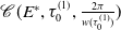


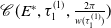
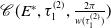


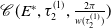
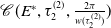
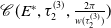
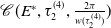


5. Bifurcation diagram
In this section, we examine the bifurcation diagram of system (1.2) in the $(\tau , K)$
-plane. By statement (2) of Lemma3.12, a transcritical bifurcation involving
$(\tau , K)$
-plane. By statement (2) of Lemma3.12, a transcritical bifurcation involving $E_K$
and
$E_K$
and $E^\ast$
occurs when
$E^\ast$
occurs when $\tau =\tau _{max}$
, i.e.,
$\tau =\tau _{max}$
, i.e., $(\tau , K)$
lies on the curve
$(\tau , K)$
lies on the curve $\mathscr{L}_c$
, defined as
$\mathscr{L}_c$
, defined as
 \begin{equation*}\mathscr{L}_c\,:\!=\, \left\{(\tau , K)\in \overline {\mathbb{R}}_+\times \mathbb{R}_+| K=\frac {ad}{cme^{-d\tau }-d}\right\} .\end{equation*}
By Corollary 3.10, there exists a sequence of bifurcation curves through which Hopf bifurcation occurs at $E^\ast$
. Let
$E^\ast$
. Let $\ell _n(\tau , K)\,:\!=\,\tau w(\tau , K)-\theta _n(\tau . K)$
. The Hopf bifurcation curve is given by
$\ell _n(\tau , K)\,:\!=\,\tau w(\tau , K)-\theta _n(\tau . K)$
. The Hopf bifurcation curve is given by
 \begin{equation*}\mathscr{L}_n= \{(\tau , K)\in \overline {\mathbb{R}}_+\times \mathbb{R}_+|\ell _n(\tau , K)=0, 0\leq \tau \lt \bar {\tau }\}, \ n=0, 1, 2, \cdots .\end{equation*}
Lemma 5.1.
Consider the curve $\mathscr{L}_0$
, i.e., the graph of
$\mathscr{L}_0$
, i.e., the graph of $\ell _0(\tau , K)=0$
.
$\ell _0(\tau , K)=0$
.
-
(1)
$\mathscr{L}_0$
lies above the curve
$\mathscr{L}_c$
. -
(2)
$\mathscr{L}_0$
starts at the point
$(\tau , K)=( 0, K_0)$
and extends to infinity, meaning
$\mathscr{L}_0$
exists for all
$K\geq K_0$
. -
(3) There exists a smooth function
$K=K(\tau )$
for
$\tau \in [0, \varepsilon )$
, where
$\varepsilon \gt 0$
is small such that
Furthermore,
\begin{equation*}K_0=K(0),\ \ \ell _0(K(\tau ), \tau )=0, \ \tau \in [0, \varepsilon ).\end{equation*}
$K'(\tau )\lt 0$
if
$cm\gt (1+\sqrt {2})d$
,
$K'(\tau )\gt 0$
if
$cm\lt (1+\sqrt {2})d$
. If
$cm=(1+\sqrt {2})d$
, then
$K''(\tau )\gt 0$
.










Proof. Statement (1) follows directly from Lemma 2.5.
(2) Since $\ell _0(0, K_0)=0-\arccos (1)=0$
, the point
$\ell _0(0, K_0)=0-\arccos (1)=0$
, the point $(0, K_0)$
serves as an endpoint of
$(0, K_0)$
serves as an endpoint of $\mathscr{L}_0$
. By Lemma 3.4, for any
$\mathscr{L}_0$
. By Lemma 3.4, for any $K\geq K_0$
,
$K\geq K_0$
, $\tau w(\tau )$
intersects
$\tau w(\tau )$
intersects $\theta _0(\tau )$
at least once. Hence, the graph of
$\theta _0(\tau )$
at least once. Hence, the graph of $\ell _0(\tau , K)=0$
exists for all
$\ell _0(\tau , K)=0$
exists for all $K\geq K_0$
.
$K\geq K_0$
.
(3) By direct calculation, we obtain
 \begin{equation*}\ell _0(0, K_0)=0, \text{and} \ \frac {\partial \ell _0(\tau , K)}{\partial K}_{|(0, K_0)}=-\frac {(cm-d)\sqrt {rd}}{mca\sqrt {c^2m^2-d^2}}\neq 0.\end{equation*}
By the implicit function theorem, there exists a function $K=K(\tau )$
for
$K=K(\tau )$
for $\tau \in [0, \varepsilon )$
, where
$\tau \in [0, \varepsilon )$
, where $\varepsilon \gt 0$
is small such that
$\varepsilon \gt 0$
is small such that $K_0=K(0)$
and
$K_0=K(0)$
and $\ell _0(K(\tau ), \tau )=0$
. Furthermore, a straightforward calculation yields
$\ell _0(K(\tau ), \tau )=0$
. Furthermore, a straightforward calculation yields
 \begin{equation*}K'(\tau )_{|\tau =0}=-\frac {mca(c^2m^2-2cmd-d^2)}{(cm-d)^2}.\end{equation*}
If $K'(\tau )_{|\tau =0}=0$
(i.e.,
$K'(\tau )_{|\tau =0}=0$
(i.e., $cm=(1+\sqrt {2})d$
), then by implicit differentiation,
$cm=(1+\sqrt {2})d$
), then by implicit differentiation, $K''(\tau )_{|\tau =0}=3\sqrt {2}ac^2m^2$
. This establishes the desired result.
$K''(\tau )_{|\tau =0}=3\sqrt {2}ac^2m^2$
. This establishes the desired result.
Bifurcation diagram in the $(\tau , K)$
-plane. The curve
$(\tau , K)$
-plane. The curve $\mathscr{L}_c$
represents the transcritical bifurcation, while
$\mathscr{L}_c$
represents the transcritical bifurcation, while $\mathscr{L}_n (n=0, 1, 2, 3)$
are curves of Hopf bifurcation. Dash lines highlight critical parameter values that are not bifurcation curves.
$\mathscr{L}_n (n=0, 1, 2, 3)$
are curves of Hopf bifurcation. Dash lines highlight critical parameter values that are not bifurcation curves.

In what follows, we will sketch the bifurcation diagram of the system (1.2) in the first quadrant of the $(\tau , K)$
plane. There are a curve of transcritical bifurcation
$(\tau , K)$
plane. There are a curve of transcritical bifurcation $\mathscr{L}_c$
and a curve of Hopf bifurcation
$\mathscr{L}_c$
and a curve of Hopf bifurcation $\mathscr{L}_0$
. By statement (3) of Lemma 5.1, in a neighbourhood of
$\mathscr{L}_0$
. By statement (3) of Lemma 5.1, in a neighbourhood of $(0, K_0)$
, the curve
$(0, K_0)$
, the curve $\mathscr{L}_0$
exhibits different monotonicity behaviours depending on whether
$\mathscr{L}_0$
exhibits different monotonicity behaviours depending on whether $cm\leq (1+\sqrt {2})d$
or
$cm\leq (1+\sqrt {2})d$
or $cm\gt (1+\sqrt {2})d$
. The simplest sketch of
$cm\gt (1+\sqrt {2})d$
. The simplest sketch of $\mathscr{L}_0$
is presented in Figure 6, ensuring minimal changes in monotonicity for
$\mathscr{L}_0$
is presented in Figure 6, ensuring minimal changes in monotonicity for $\tau \in [0, \check {\tau })$
.
$\tau \in [0, \check {\tau })$
.
The two curves $\mathscr{L}_c$
and
$\mathscr{L}_c$
and $\mathscr{L}_0$
divide the first quadrant of
$\mathscr{L}_0$
divide the first quadrant of $(\tau , K)$
-plane into three regions
$(\tau , K)$
-plane into three regions $V_a$
,
$V_a$
, $V_b$
, and
$V_b$
, and $V_c$
, defined as follows:
$V_c$
, defined as follows:
 \begin{eqnarray*} &&V_a=\{(\tau , K)\in \overline {\mathbb{R}}_+\times \mathbb{R}_+| \ell _0(\tau , K)\gt , 0\leq \tau \lt \bar {\tau }\},\\ &&V_b=\{(\tau , K)\in \overline {\mathbb{R}}_+\times \mathbb{R}_+|\ell _0(\tau , K)\lt 0, 0\leq \tau \lt \bar {\tau }\}, V_c=\{(\tau , K)\in \overline {\mathbb{R}}_+\times \mathbb{R}_+|\tau \gt \tau _{max}\}. \end{eqnarray*}
By Theorem4.5, $E_K$
is globally asymptotically stable for
$E_K$
is globally asymptotically stable for $(K, \tau )\in V_c$
, and system (1.2) undergoes a transcritical bifurcation for
$(K, \tau )\in V_c$
, and system (1.2) undergoes a transcritical bifurcation for $(K, \tau )\in \mathscr{L}_c$
.
$(K, \tau )\in \mathscr{L}_c$
. $E^\ast$
is locally asymptotically stable for
$E^\ast$
is locally asymptotically stable for $(K, \tau )\in V_b$
, then system (1.2) experiences a Hopf bifurcation for
$(K, \tau )\in V_b$
, then system (1.2) experiences a Hopf bifurcation for $(K, \tau )\in \mathscr{L}_0$
.
$(K, \tau )\in \mathscr{L}_0$
. $E^\ast$
is unstable for
$E^\ast$
is unstable for $(K, \tau )\in V_a$
, and a periodic solution exists for
$(K, \tau )\in V_a$
, and a periodic solution exists for $(K, \tau )$
in a tubular neighbourhood of
$(K, \tau )$
in a tubular neighbourhood of $\mathscr{L}_0$
.
$\mathscr{L}_0$
.
The existence of additional Hopf bifurcation curves $\mathscr{L}_n (n=1, 2, {\cdots}\,)$
depends on the choice of parameters. If such curves exist, they are positioned above
$\mathscr{L}_n (n=1, 2, {\cdots}\,)$
depends on the choice of parameters. If such curves exist, they are positioned above $\mathscr{L}_0$
and do not intersect any other Hopf bifurcation curve. Numerical studies suggest two possible topological structures for
$\mathscr{L}_0$
and do not intersect any other Hopf bifurcation curve. Numerical studies suggest two possible topological structures for $\mathscr{L}_n$
:
$\mathscr{L}_n$
: $\mathscr{L}_n\simeq \mathbb{R}$
, or
$\mathscr{L}_n\simeq \mathbb{R}$
, or $\mathscr{L}_n\simeq \mathbb{S}^1$
, where
$\mathscr{L}_n\simeq \mathbb{S}^1$
, where $\simeq$
means “is topologically isomorphic”. Figure 6 illustrates an example where
$\simeq$
means “is topologically isomorphic”. Figure 6 illustrates an example where $\mathscr{L}_1\simeq \mathbb{R}$
,
$\mathscr{L}_1\simeq \mathbb{R}$
, $\mathscr{L}_2\simeq \mathbb{R}$
,
$\mathscr{L}_2\simeq \mathbb{R}$
, $\mathscr{L}_3\simeq \mathbb{S}^1$
.
$\mathscr{L}_3\simeq \mathbb{S}^1$
.
The region $V_a$
is divided into several subregions by the Hopf bifurcation curves
$V_a$
is divided into several subregions by the Hopf bifurcation curves $\mathscr{L}_n (n=1, 2, {\cdots}\,)$
. Whenever
$\mathscr{L}_n (n=1, 2, {\cdots}\,)$
. Whenever $(K, \tau )$
crosses
$(K, \tau )$
crosses $\mathscr{L}_n$
, the Hopf bifurcation occurs, and a periodic solution emerges in a tubular neighbourhood of
$\mathscr{L}_n$
, the Hopf bifurcation occurs, and a periodic solution emerges in a tubular neighbourhood of $\mathscr{L}_n$
. For
$\mathscr{L}_n$
. For $K\lt K_0$
, if
$K\lt K_0$
, if $\mathscr{L}_n (n=2, 3, {\cdots}\,)$
transversally intersects the horizontal line exactly twice, by Theorem4.6, the connected components
$\mathscr{L}_n (n=2, 3, {\cdots}\,)$
transversally intersects the horizontal line exactly twice, by Theorem4.6, the connected components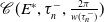 $\mathscr{C}\,(E^*,\tau _n^{-}, \frac {2\pi }{w(\tau _n^{-})})$
and
$\mathscr{C}\,(E^*,\tau _n^{-}, \frac {2\pi }{w(\tau _n^{-})})$
and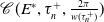 $\mathscr{C}\,(E^*,\tau _n^{+}, \frac {2\pi }{w(\tau _n^{+})})$
coincide. That is, a periodic solution emerging at
$\mathscr{C}\,(E^*,\tau _n^{+}, \frac {2\pi }{w(\tau _n^{+})})$
coincide. That is, a periodic solution emerging at $(\tau _n^-, K)$
will terminate at
$(\tau _n^-, K)$
will terminate at $(\tau _n^+, K)$
. Determining the number of periodic solutions within the subregions between successive Hopf bifurcation curves is challenging. This is due to the potential presence of other bifurcations affecting periodic solutions. Even in the absence of such bifurcations, tracing the periodic solutions as
$(\tau _n^+, K)$
. Determining the number of periodic solutions within the subregions between successive Hopf bifurcation curves is challenging. This is due to the potential presence of other bifurcations affecting periodic solutions. Even in the absence of such bifurcations, tracing the periodic solutions as $(\tau , K)$
crosses
$(\tau , K)$
crosses $\mathscr{L}_n (n=0, 1, 2 {\cdots}\,)$
remains difficult, as there is no definitive criterion for predicting the onset and termination of connected components in global Hopf bifurcation when
$\mathscr{L}_n (n=0, 1, 2 {\cdots}\,)$
remains difficult, as there is no definitive criterion for predicting the onset and termination of connected components in global Hopf bifurcation when $K\gt K_0$
or
$K\gt K_0$
or $\chi (n)\gt 2$
.
$\chi (n)\gt 2$
.
Remark 5.2. The bifurcation diagram in Figure 6 is not complete, as there may exist additional bifurcation curves of periodic solutions, such as saddle-node bifurcations of limit cycles and period-doubling bifurcations. A detailed investigation of these bifurcations is beyond the scope of this work.
Remark 5.3.
If $cm\gt (1+\sqrt {2})d$
, define
$cm\gt (1+\sqrt {2})d$
, define
 \begin{equation*}\tau ^\ast =\arg \min _{\tau \in (0, \bar {\tau })}\{\ell _0(\tau , K_0)=0\}.\end{equation*}
Then, for any point $(\tau , K)\in \mathscr{L}_0$
with
$(\tau , K)\in \mathscr{L}_0$
with $0\lt \tau \lt \tau ^\ast$
, we have
$0\lt \tau \lt \tau ^\ast$
, we have $K\lt K_0$
(see Figure 6 (b)).
$K\lt K_0$
(see Figure 6 (b)).
Biological significance of $\tau ^\ast$
. Predator–prey coexistence via oscillatory patterns can occur at lower environmental carrying capacities when delay (
$\tau ^\ast$
. Predator–prey coexistence via oscillatory patterns can occur at lower environmental carrying capacities when delay ( $\tau \gt 0$
) is introduced, compared to scenarios without delay (
$\tau \gt 0$
) is introduced, compared to scenarios without delay ( $\tau = 0$
) under the condition that
$\tau = 0$
) under the condition that $(1+\sqrt {2})d\lt cm$
, and
$(1+\sqrt {2})d\lt cm$
, and $0\lt \tau \lt \tau ^\ast$
. The significance of
$0\lt \tau \lt \tau ^\ast$
. The significance of $\tau ^\ast$
will be further illustrated in the next section.
$\tau ^\ast$
will be further illustrated in the next section.
6. Discussion
The classical predator–prey model with Holling type II functional response typically exhibits relatively simple dynamical behaviour. By contrast, the incorporation of a maturation delay introduces significantly richer dynamics and provides a more realistic framework for modelling predator–prey interactions observed in nature. In this section, we interpret the effects of delay on population persistence and oscillatory coexistence.
-
• Threshold dynamics for prey–predator coexistence.
The coexistence of prey and predators requires
$\tau \lt \tau _{\max }$
, which is equivalent to
$K\gt K_1$
. Hereand thus
\begin{equation*} K_1=\frac {ad}{cme^{-d\tau }-d}, \end{equation*}
As
\begin{equation*} K_1\gt \frac {ad}{cme^{-d\tau }-d}\Big |_{\tau =0}=K_c. \end{equation*}
$\tau$
increases,
$K_1$
increases, meaning that a higher environmental carrying capacity is needed for both species to coexist. This threshold is illustrated by the transcritical bifurcation curve
$\mathscr{L}_c$
in Figure 6, together with the critical values
$K_1$
and
$K_c$
shown in Figure 7. Biologically, this behaviour is intuitive: larger delays reduce predator survival (
$e^{-d\tau }$
), forcing predators to rely on greater prey abundance to compensate for mortality. As a consequence, prey populations face stronger predation pressure.
-
• Oscillatory dynamics of prey and predator populations.
Oscillatory dynamics emerge once the condition
$\ell _0(\tau , K)\gt 0$
is satisfied. A secondary threshold involving the predator death rate further determines whether sustained oscillations are possible.-
1. If
$cm\leq (1+\sqrt {2})d$
, predator mortality is relatively high, leading to low survival
$e^{-d\tau }$
. In this case, predators require more prey to maintain oscillations. Since survival decreases as
$\tau$
increases, the critical carrying capacity rises monotonically with
$\tau$
. This behaviour is reflected by the monotone increase of
$\mathscr{L}_0$
in Figure 6(a). -
2. If
$cm\gt (1+\sqrt {2})d$
, predator mortality is comparatively low, yielding higher survival rates. For small delays
$\tau \in (0,\tau ^\ast )$
, oscillatory coexistence can be sustained at lower values of
$K$
. However, once
$\tau$
exceeds
$\tau ^\ast$
(with
$\tau \in (\tau ^\ast ,\bar {\tau })$
), survival declines sufficiently to require larger
$K$
values for oscillations to persist. This non-monotone behaviour of
$\mathscr{L}_0$
is illustrated in Figure 6(b), with
$\tau ^\ast$
defined in Remark 5.3.
-








Global Hopf bifurcation and connected components as functions of $K$
for
$K$
for $\tau \gt \tau ^\ast$
. The orange dot corresponds to the transcritical bifurcation threshold
$\tau \gt \tau ^\ast$
. The orange dot corresponds to the transcritical bifurcation threshold $K_1$
, while the red dots denote the Hopf bifurcation thresholds
$K_1$
, while the red dots denote the Hopf bifurcation thresholds $K_h^{(i)}$
(
$K_h^{(i)}$
( $i=1,2,\ldots ,10$
). The location of
$i=1,2,\ldots ,10$
). The location of $K_h^{(1)}$
for
$K_h^{(1)}$
for $\tau \in (0,\tau ^\ast )$
is indicated by “
$\tau \in (0,\tau ^\ast )$
is indicated by “ $\color {red}{\ast }$
”. Critical values
$\color {red}{\ast }$
”. Critical values $K_c$
and
$K_c$
and $K_0$
denote the transcritical and Hopf bifurcation thresholds of the ODE model (
$K_0$
denote the transcritical and Hopf bifurcation thresholds of the ODE model ( $\tau =0$
). Detailed descriptions are provided in this section.
$\tau =0$
). Detailed descriptions are provided in this section.

To illustrate these effects, consider the bifurcation diagram of Figure 7, where $K$
is treated as the bifurcation parameter. Fixing
$K$
is treated as the bifurcation parameter. Fixing $\tau =26$
,
$\tau =26$
, $r=30$
,
$r=30$
, $m=1$
,
$m=1$
, $c=4$
,
$c=4$
, $d=0.1$
, and
$d=0.1$
, and $a=1$
, we have
$a=1$
, we have $cm\gt (1+\sqrt {2})d$
and
$cm\gt (1+\sqrt {2})d$
and $\tau \gt \tau ^\ast =24.1$
. The critical bifurcation values are
$\tau \gt \tau ^\ast =24.1$
. The critical bifurcation values are
 \begin{align*} K_c=0.25,\quad K_1=0.51,\quad K_0=1.0512,\quad K_h^{(1)}=1.328,\quad K_h^{(2)}=1.54,\quad K_h^{(3)}=1.67,\quad K_h^{(4)}=1.76,\\[5pt]K_h^{(5)}=1.85,\quad K_h^{(6)}=1.994,\quad K_h^{(7)}=2.135,\quad K_h^{(8)}=2.3956,\quad K_h^{(9)}=2.7395,\quad K_h^{(10)}=3.996. \end{align*}
As $K$
increases, system (1.2) undergoes a transcritical bifurcation at
$K$
increases, system (1.2) undergoes a transcritical bifurcation at $K=K_1$
and a sequence of Hopf bifurcations at
$K=K_1$
and a sequence of Hopf bifurcations at $K=K_h^{(i)}$
. In particular,
$K=K_h^{(i)}$
. In particular, $K_h^{(1)}\gt K_0$
and
$K_h^{(1)}\gt K_0$
and $K_1\gt K_c$
, showing that delay increases the environmental resources needed for both coexistence and oscillatory dynamics.
$K_1\gt K_c$
, showing that delay increases the environmental resources needed for both coexistence and oscillatory dynamics.
When $\tau$
decreases into the interval
$\tau$
decreases into the interval $\tau \in (0,\tau ^\ast )$
, the first Hopf bifurcation threshold
$\tau \in (0,\tau ^\ast )$
, the first Hopf bifurcation threshold $K_h^{(1)}$
shifts to the position marked “
$K_h^{(1)}$
shifts to the position marked “ $\color {red}{\ast }$
” between
$\color {red}{\ast }$
” between $K_1$
and
$K_1$
and $K_0$
in Figure 7. This indicates that smaller delays may allow oscillatory coexistence with fewer resources.
$K_0$
in Figure 7. This indicates that smaller delays may allow oscillatory coexistence with fewer resources.
In summary, our results show that maturation delay is not uniformly detrimental. While increasing delay generally reduces effective recruitment through mortality during development (captured by the survival factor $e^{-d\tau }$
), we also identify a counterintuitive regime in which small delays can promote predator persistence by enabling oscillatory coexistence at lower carrying capacities. This switch is organized by a critical timescale
$e^{-d\tau }$
), we also identify a counterintuitive regime in which small delays can promote predator persistence by enabling oscillatory coexistence at lower carrying capacities. This switch is organized by a critical timescale $\tau ^\ast$
, which separates two qualitatively different outcomes: for
$\tau ^\ast$
, which separates two qualitatively different outcomes: for $\tau \gt \tau ^\ast$
the demographic cost dominates and delay increases the carrying-capacity requirements for both predator persistence and sustained oscillations, whereas for
$\tau \gt \tau ^\ast$
the demographic cost dominates and delay increases the carrying-capacity requirements for both predator persistence and sustained oscillations, whereas for $\tau \in (0,\tau ^\ast )$
modest delay can facilitate cyclic coexistence under tighter resource constraints.
$\tau \in (0,\tau ^\ast )$
modest delay can facilitate cyclic coexistence under tighter resource constraints.
A plausible explanation for this counterintuitive behaviour arises when $cm\gt (1+\sqrt {2})d$
. In the delay-free model, predator recruitment is strongly and nearly instantaneously coupled to current prey abundance, which stabilizes the coexistence equilibrium over a broad parameter range and postpones oscillations until enrichment is sufficiently large (in particular, until
$cm\gt (1+\sqrt {2})d$
. In the delay-free model, predator recruitment is strongly and nearly instantaneously coupled to current prey abundance, which stabilizes the coexistence equilibrium over a broad parameter range and postpones oscillations until enrichment is sufficiently large (in particular, until $K$
exceeds
$K$
exceeds $K_0$
). Introducing a small maturation delay weakens this tight coupling by spreading recruitment over recent past prey conditions. Biologically, predator reproduction becomes less synchronized with current prey density and more influenced by prey availability during the recent past. As a result, the predator response is effectively smoothed and shifted in time: recruitment rises more slowly when prey increase and can remain elevated briefly after prey begin to decline. This timing shift can destabilize an equilibrium that is stable without delay, thereby generating self-sustained oscillations without requiring as much enrichment. Beyond
$K_0$
). Introducing a small maturation delay weakens this tight coupling by spreading recruitment over recent past prey conditions. Biologically, predator reproduction becomes less synchronized with current prey density and more influenced by prey availability during the recent past. As a result, the predator response is effectively smoothed and shifted in time: recruitment rises more slowly when prey increase and can remain elevated briefly after prey begin to decline. This timing shift can destabilize an equilibrium that is stable without delay, thereby generating self-sustained oscillations without requiring as much enrichment. Beyond $\tau ^\ast$
, however, further delay increasingly penalizes recruitment, and the system again requires higher carrying capacity to sustain oscillations and maintain predator persistence.
$\tau ^\ast$
, however, further delay increasingly penalizes recruitment, and the system again requires higher carrying capacity to sustain oscillations and maintain predator persistence.
Acknowledgements
The authors would like to thank two anonymous referees for careful reading and insightful comments, which greatly improve the manuscript. We used ChatGPT to polish some of the writing.
Funding statement
The research of C. Shan was partially supported by Simons Foundation-Collaboration Grants for Mathematicians 523360. The research of H. Wang was partially supported by the Natural Sciences and Engineering Research Council of Canada (Individual Discovery Grant RGPIN-2025-05734 and Discovery Accelerator Supplement Award RGPAS-2020-00090) and the Canada Research Chairs program (Tier 1 Canada Research Chair Award).
Competing interests
The authors declare that they have no conflicts of interest.
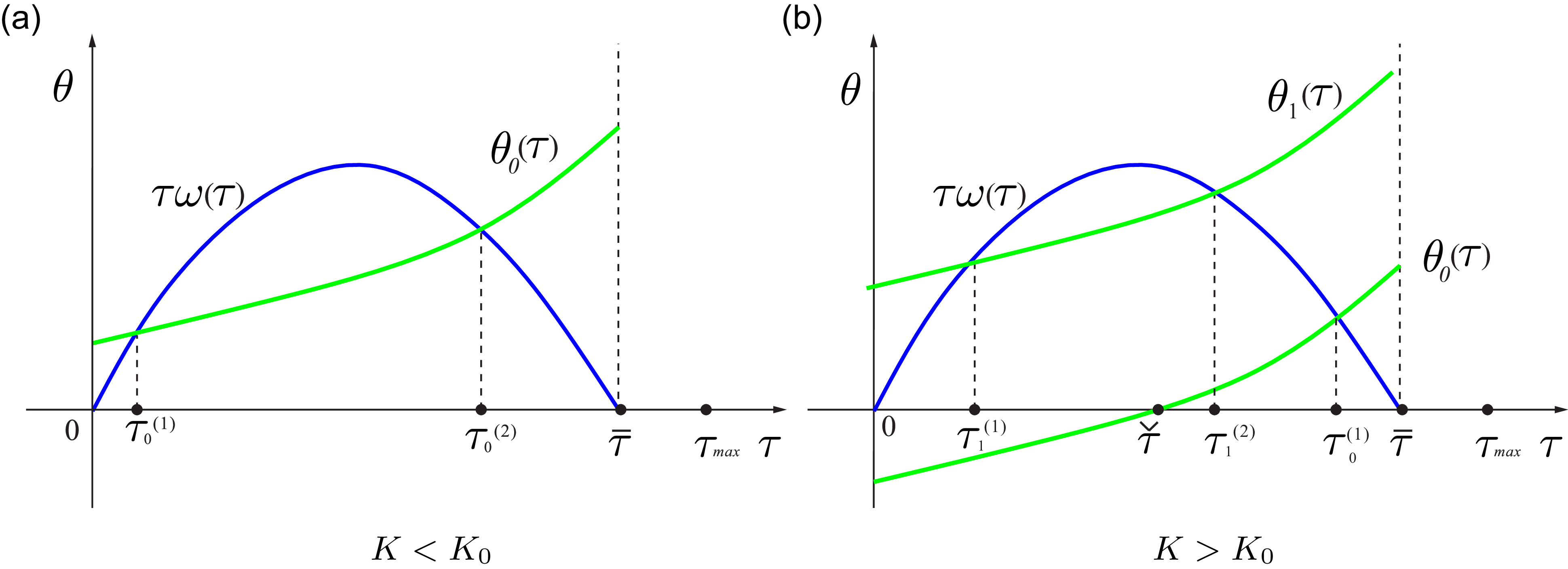


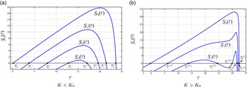


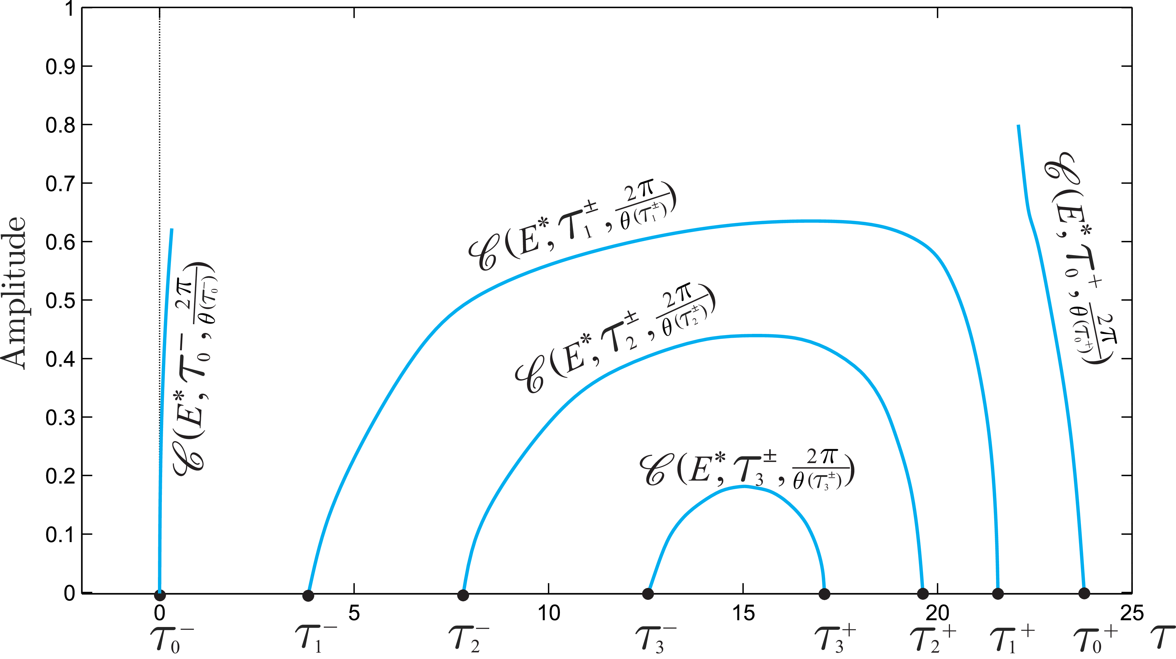


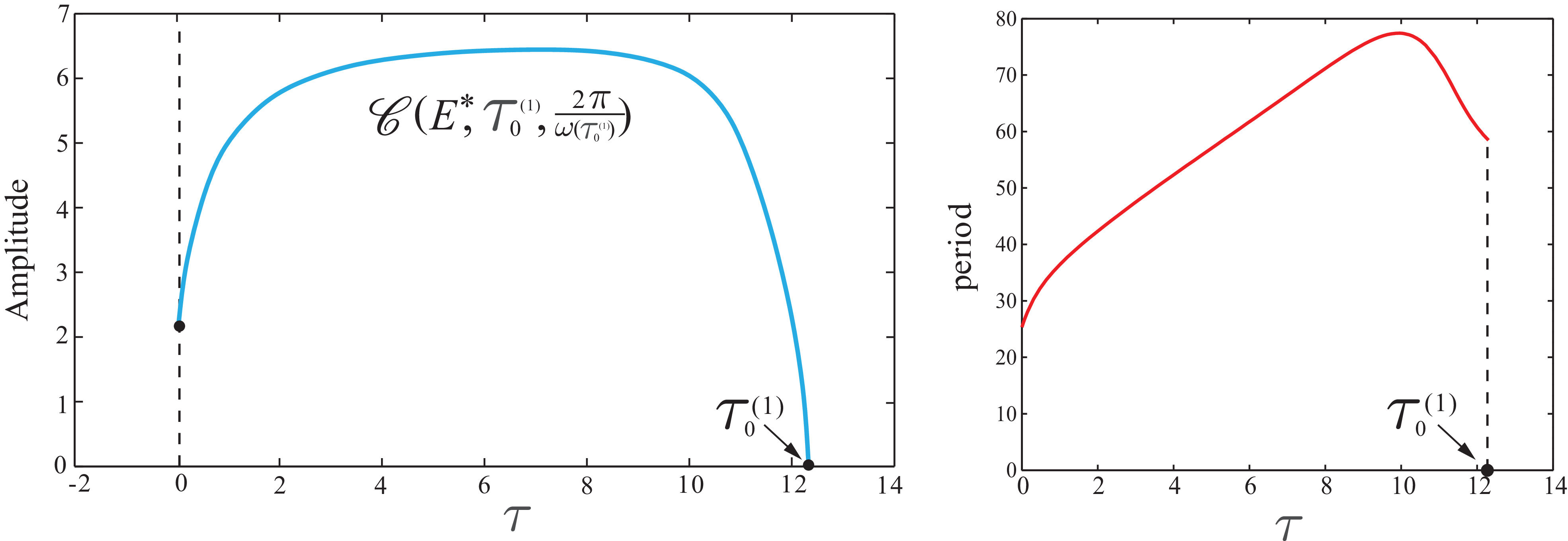


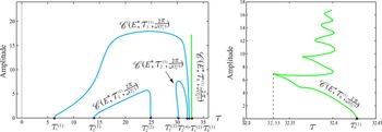


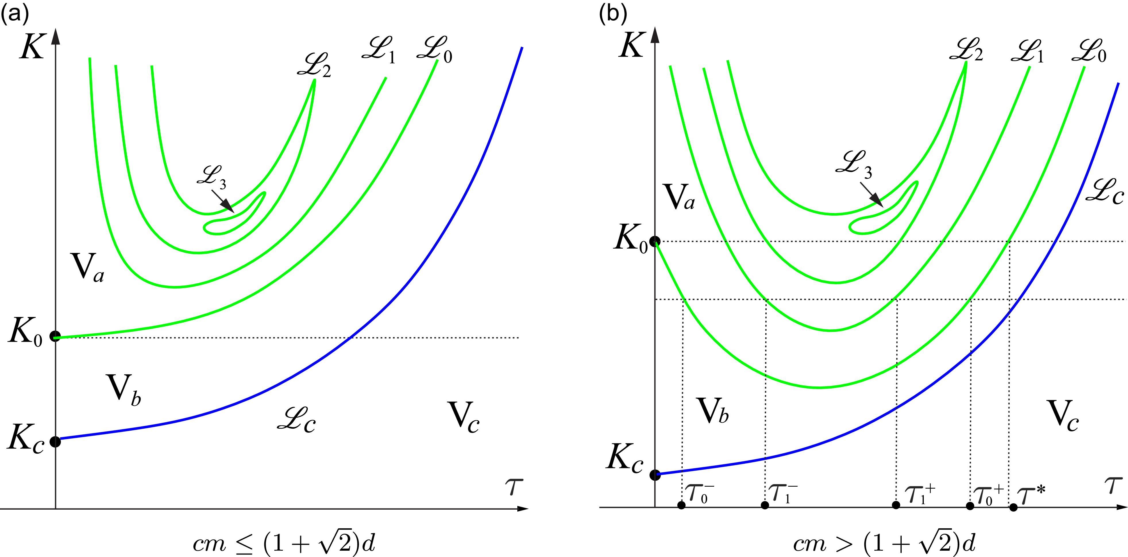


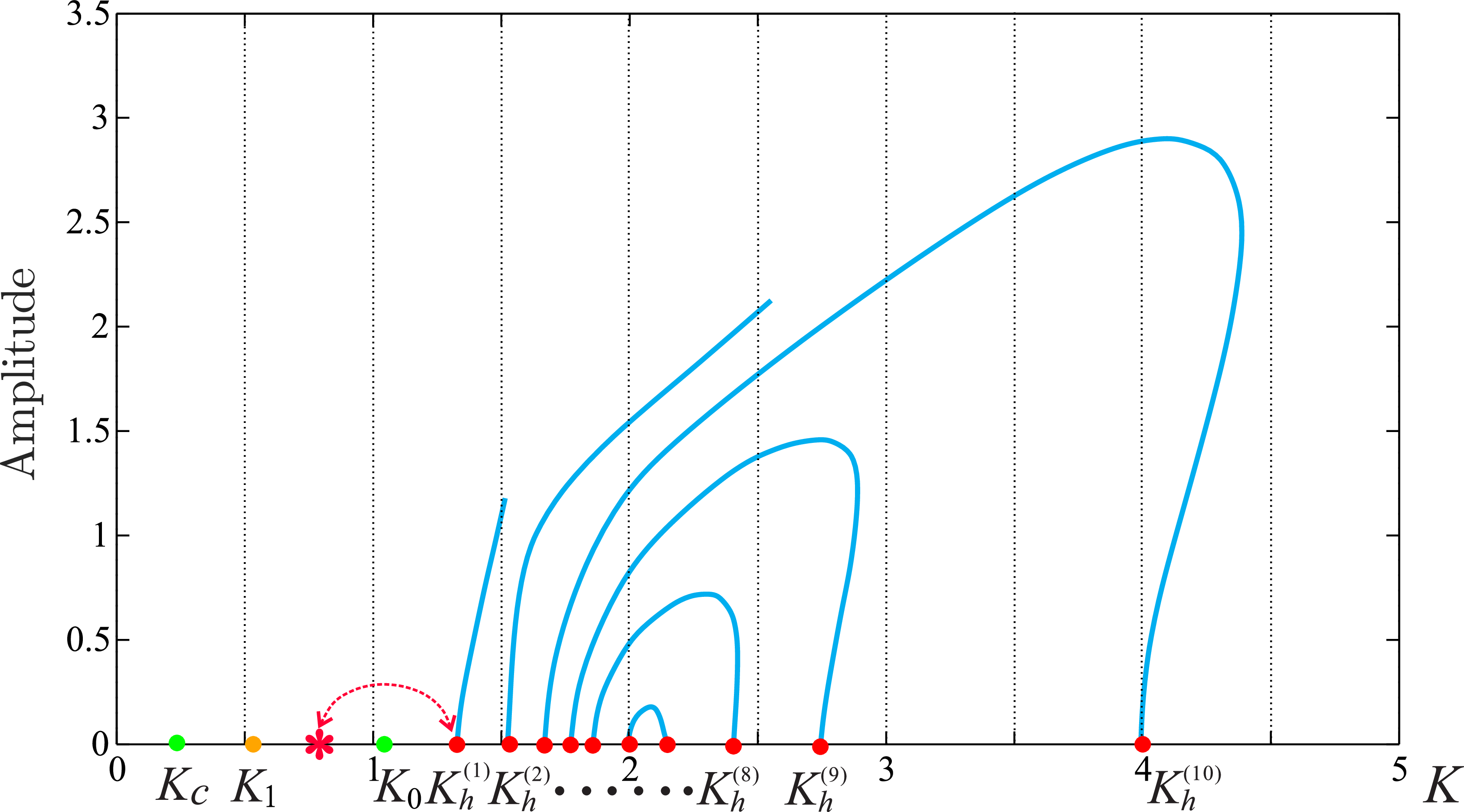


 Open access

