





Introduction
Ice sheets, which are a major factor in the world’s climate system, have become an increasing focus of research, as understanding the processes that regulate their behavior is important for assessing and predicting global climate change. In recent decades, the Antarctic Ice Sheet has experienced significant mass loss that has contributed to a continuous rise in sea level (DeConto and Pollard, Reference DeConto and Pollard2016; Rignot and others, Reference Rignot, Mouginot, Scheuchl, van den Broeke, van Wessem and Morlighem2019). Estimations indicate that within the next 30 years, global sea level may rise by more than 20 cm in coastal areas (Jevrejeva and others, Reference Jevrejeva, Jackson, Riva, Grinsted and Moore2016). An accurate assessment of glacier changes and their melting processes may help develop strategies for mitigating flooding and adjust urban planning in cities endangered by rising sea levels (Hinkel and others, Reference Hinkel2014). Moreover, the albedo effect of glaciers plays a significant role in the Earth’s energy balance, especially in the age of global warming (Benn and Evans, Reference Benn and Evans2010). Changes in the atmosphere reduce humidity in polar areas and, as a result, limit the accumulation of snow, further affecting the glacier dynamics (Trusel and others, Reference Trusel2018). There is thus a need for a better understanding of the processes shaping glaciers and influencing their conditions.
One of the main indicators of the condition of a glacier is the grounding line (GL), which is defined as the boundary between the grounded ice sheet and the floating ice shelf detached from the land surface (Weertman, Reference Weertman1974). The identification of the GL is crucial for estimating the glacier’s mass balance, including the basal melting and ice/snow accumulation (Fricker and Padman, Reference Fricker and Padman2006; Fricker and others, Reference Fricker, Coleman, Padman, Scambos, Bohlander and Brunt2009; Smith and others, Reference Smith2020). The retreating GL reduces frictional resistance between the ice sheet and the bedrock, which allows for increased ice discharge, facilitates the intrusion of warm ocean waters beneath the ice shelf and consequently accelerates basal melting. In critical locations, such retreat may lead to the unpinning of ice shelves, further destabilizing the system (Pattyn and others, Reference Pattyn, Huyghe, De Brabander and De Smedt2006; Holland and others, Reference Holland, Thomas, De Young, Ribergaard and Lyberth2008; Brondex and others, Reference Brondex, Gagliardini, Gillet-Chaulet and Durand2017). Recent studies have shown that the spatial extent and volume of the ice cover have been significantly reduced as a result of the melting process that occurs at the glacier base, due to its contact with warmer waters (Mouginot and others, Reference Mouginot2019; Jourdain and others, Reference Jourdain, Mathiot, Burgard, Caillet and Kittel2022). For example, research conducted in West Antarctica indicates a significant acceleration of glacier melt and GL retreat (Joughin and others, Reference Joughin, Smith and Medley2014; Shepherd and others, Reference Shepherd2018). Similar results have also been observed in other regions, including East Antarctica and Greenland (Shepherd and others, Reference Shepherd2018; Mouginot and others, Reference Mouginot2019). The most recent global analyses further demonstrate the extent of the process of GL retreat and associated ice mass loss in recent decades (Otosaka and others, Reference Otosaka2023).
As the position of the GL varies with time, it is often referred to as the grounding zone (GZ). We define it as the difference between the maximum and minimum migration ranges within a year. The width of the GZ is related to the tidal changes non-linearly, which results in tenfold greater GL migration from hydrostatic equilibrium (HE) during tidal rise than during the tidal fall (Tsai and Gudmundsson, Reference Tsai and Gudmundsson2015). The migration also depends on the slope of the bed and the ice surface, as a lower slope inclination facilitates water penetration under the glacier, increasing the migration range. However, recent studies have revealed that the actual GZ is much larger than the maximum zone calculated from the HE. Potential factors include: bedrock hardness (Chen and others, Reference Chen, Rignot, Scheuchl and Ehrenfeucht2023), deep water intrusions (Rignot and others, Reference Rignot, Ciracì, Scheuchl, Tolpekin, Wollersheim and Dow2024), cavities below the ice (Milillo and others, Reference Milillo2022) or retrograde bed slope (Antropova and others, Reference Antropova, Mueller, Samsonov, Komarov, Bonneau and Crawford2024). The exact role of the above phenomena in glacier dynamics has not yet been fully understood and requires further research on GL behavior.
Accurate determination of the GL position is problematic mainly due to its location beneath the glacier, and the measurement precision remains low (Horgan and Anandakrishnan, Reference Horgan and Anandakrishnan2006). Recent popular methods for monitoring the GL migration are based on remote sensing data. These data are useful because they cover extensive areas of land, and their acquisition does not require any in situ instruments. Recent developments in the field of remote sensing include repeat track laser-altimetry (RTLA) (e.g., Brunt and others, Reference Brunt, Fricker, Padman, Scambos and O’Neel2010b), differential range offset tracking (e.g., Christianson and others, Reference Christianson2016; Joughin and others, Reference Joughin, Shean, Smith and Dutrieux2016) and pseudo crossover radar-altimetry (e.g., Dawson and Bamber, Reference Dawson and Bamber2017). Another promising approach leverages Sentinel-1 synthetic aperture radar (SAR) images. The technique is based on differential interferometric synthetic aperture radar (DInSAR), widely regarded as the most effective and precise remote sensing method for GL detection (Rignot and others, Reference Rignot, Mouginot and Scheuchl2011; Friedl and others, Reference Friedl, Weiser, Fluhrer and Braun2020). It allows glacier surface changes to be monitored with high resolution, even in darkness and cloudy conditions, and is thus advantageous in polar regions (Nagler and others, Reference Nagler, Rott, Hetzenecker, Wuite and Potin2015). The DInSAR method enables displacement measurements with a theoretical precision down to several centimeters (Hanssen, Reference Hanssen2001). As a result, the GL position can be identified with a precision of up to 100 m (Rosier and others, Reference Rosier, Marsh, Rack, Gudmundsson, Wild and Ryan2017). Other advantages include the ability to measure large areas in a single session and the repeatability provided by consecutive satellite acquisitions. Although such a perspective is important in analyzing the dynamics of glaciers and assessing their condition, to date, only a few studies have been based on data from multi-year time series or have explored temporary movements within the GZ (e.g., Tympalski and others, Reference Tympalski, Sompolski, Kopeć and Milczarek2024; Zhu and others, Reference Zhu, Hogg, Hooper and Wallis2025).
This paper describes how data from the Sentinel-1 mission can be used to assess temporary changes in GL position, and as such represents a novel approach in the analysis of glacier dynamics. The research presented here employs SAR interferometry and machine learning algorithms to detect GL positions over a 4.5 year period. We utilize such time series to test the assumption of maximum migration ranges and to attempt pattern recognition in temporal GL migration. It thus describes how existing tools can be used in novel applications with an aim to better understand glacier dynamics and ultimately contribute to future research on global climate change.
Study area
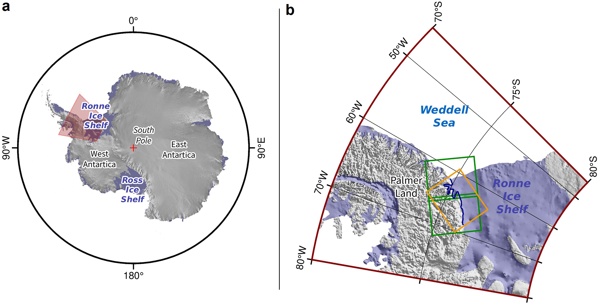
The choice of the study area was dictated by the fact that the West Antarctic Ice Sheet has experienced the highest mass loss in recent decades (Otosaka and others, Reference Otosaka2023). The area was defined around the Orville Coast, which is the western part of the Ronne Ice Shelf (Fig. 1). Previous research in this area has focused only on the geological signs of the extent of the past ice cover (Carrara, Reference Carrara1981). Although the GL position for this area has been identified in several studies (i.e., in delineation projects concerning the entire Antarctic (Rignot and others, Reference Rignot, Mouginot and Scheuchl2016; Floricioiu and others, Reference Floricioiu, Krieger, Chowdhury and Bässler2021)), it has never been an independent object of dedicated analyses. The Orville Coast was chosen due to several characteristics that make it conducive to monitor GL migration. One of the key reasons is relatively low ice velocity in this region (Rignot and others, Reference Rignot, Mouginot and Scheuchl2016), which is advantageous because high-rate horizontal ice movement (associated with glacier flow) might lead to decorrelation and introduce additional noise. As a consequence, the boundary between the ice sheet and the ice shelf could be blurred in interferograms (Tympalski and others, Reference Tympalski, Sompolski, Kopeć and Milczarek2024). This problem is particularly relevant in areas with multiple tributaries, where the glacier flow velocity is not only high but also perpendicular to the GL direction.
Location of the Orville Coast. (a) The location of the study area in Antarctica indicated by the red trapezoid; (b) zoom on the fragment indicated with the red trapezoid on panel (a). The blue line indicates the Orville Coast, and the rectangles show the coverage of the acquired Sentinel-1 data: the green rectangles correspond to the descending path No. 37 (frame Nos. 856 and 862), and the orange rectangle corresponds to the ascending path No. 49 (frame No. 909). EPSG: 4326.

Another reason is the unique topography of the Orville Coast: its long coastline with only a few tributaries is expected to preserve higher coherence, thereby reducing phase noise in the interferograms. The presence of the bay in the northernmost part is further advantageous, allowing us to investigate the influence of the shoreline shape on the quality of the obtained results. In most studies, the GL position is analyzed perpendicular to the main flow direction, where migration is typically largest and thus most informative for assessing whether a glacier is retreating. In contrast, our objective is to characterize migration patterns. For this purpose, a peripheral area with simple topography is expected to exhibit smaller and more consistent migration, providing a more stable basis for identifying temporal patterns. The area is also dominated by prograde slopes of the bedrock (Frémand and others, Reference Frémand2023), which are expected to render the migration process more predictable and cause deep-water intrusions to have a smaller impact. The available data also indicate that the GZ width in this area is stable (Brunt and others, Reference Brunt, Fricker, Padman and O’Neel2010a; Rignot and others, Reference Rignot, Mouginot and Scheuchl2016), which facilitates the recognition of patterns in GL migration. Furthermore, while most of Antarctica typically has data coverage from only a single Sentinel-1 path, nearly the entire Orville Coast is covered by data from two paths (ascending and descending), which may significantly improve the temporal resolution of our results, potentially to less than 1 week. The selected study area might help obtain reliable results, verify the above-listed assumptions and reduce the disadvantages of our previous research (Tympalski and others, Reference Tympalski, Sompolski, Kopeć and Milczarek2024), where complex topography and highly dynamic ice flow posed significant challenges to consistent GL detection. Overall, this configuration is expected to yield more stable and reliable delineation results, providing a solid basis for our 4.5 year analysis of the GL migration.
Materials and methods
Data coverage
This research is based on a comprehensive series of SAR data from two Sentinel-1 paths, with their extent shown in Fig. 1b. The investigated period was dictated by the availability of satellite data, as a proper interferogram requires high coherence between two SAR images. In our previous research, we identified high-velocity flow and the incidence of tributaries as two sources of disturbance (Tympalski and others, Reference Tympalski, Sompolski, Kopeć and Milczarek2024). Another common problem is the melting of the top layer (Yu and others, Reference Yu, Liu, Jezek, Warner and Wen2010; Hogg and others, Reference Hogg, Shepherd, Gourmelen and Engdahl2016), which poses a challenge for every study dedicated to ice cover. The influence of all these effects increases with the time interval between SAR data acquisitions (Bamler and Hartl, Reference Bamler and Hartl1998), and therefore, the lack of available data with shorter time intervals is the main limitation to the DInSAR approach for GL detection (Friedl and others, Reference Friedl, Weiser, Fluhrer and Braun2020).
Our time series have been adjusted to match the Sentinel-1 data in 6 day intervals. As higher temporal resolution typically translates into stronger coherence between two images, it is recommended to use data from both satellites of the Sentinel-1 constellation. The descending path (No. 37) was available in that area starting from February 2017 for Sentinel-1A, and starting from June 2017 for Sentinel-1B. The ascending path (No. 49) was available for both satellites starting from May 2019. The data from Sentinel-1B were available until its failure in December 2021. Such temporal coverage is expected to mitigate the impact of potential anomalies and prevent misleading conclusions based on single annual or short-term results. The extensive spatial coverage allows a reliable interpretation of the observed changes and processes. In addition, the combination of data from two different satellite paths further enhances the analysis by allowing a comparison of results derived from two independent data sources. Thus, although the descending path covers the entire 5 year study period and the ascending path spans only half of it, the entire set is sufficiently large for this research. Details of the acquired data are presented in Table 1. The trajectory of the ascending path is nearly perpendicular to the GL and one frame (No. 909) was sufficient to cover almost the entire study area. The descending path is approximately parallel to the GL and necessitated the use of two frames (Nos. 856 and 862). In order to optimize memory allocation, they were merged into one image corresponding to the day of acquisition. This study was conducted using a total of 404 Sentinel-1 SAR images.
Characteristics of the acquired data.

* For each frame.
Grounding line delineation
The simple DInSAR approach is a set of calculations resulting in an interferogram, defined as the signal phase difference between two satellite acquisitions, which can be subsequently recalculated as ground displacements in the satellite line-of-sight direction (Rosen and others, Reference Rosen2000; Hanssen, Reference Hanssen2001). For the purpose of GL delineation, it was adapted as a double-difference (DDInSAR, also known as a four-pass) method. The principle behind it is to differentiate two interferograms (AB–CD, with AB and CD representing interferograms based on images acquired at 6 day intervals, with C acquired 6 days after B) (Rignot and MacAyeal, Reference Rignot and MacAyeal1998). It is also possible to use only three acquisitions to obtain a single double-difference interferogram (AB–BC). In fact, at the initial stage of our research, we relied on both three-pass and four-pass interferograms. However, based on the visual inspection of the preliminary results, we determined that the four-pass variant yielded significantly better visual quality of the results. Therefore, we relied solely on the four-pass approach to maximize result quality and to avoid generating duplicate measurements for the same acquisition date (as would be the case when using both three-pass and four-pass interferograms). We recognize, however, that the optimal choice between these two approaches might depend on the specific region and processing methods. The double-difference method aims to minimize horizontal displacements resulting from glacier movement and expose primarily vertical displacements resulting from tidal changes (Rignot, Reference Rignot1996). As a result, the method allows the identification of a hinge/flexure line, which is the landward limit of vertical movement detectable at the surface (Holdsworth, Reference Holdsworth1969; Fricker and others, Reference Fricker, Coleman, Padman, Scambos, Bohlander and Brunt2009). Although the flexure line is usually located slightly farther landward, it serves as a valid representation of the GL position (Vaughan, Reference Vaughan1994).
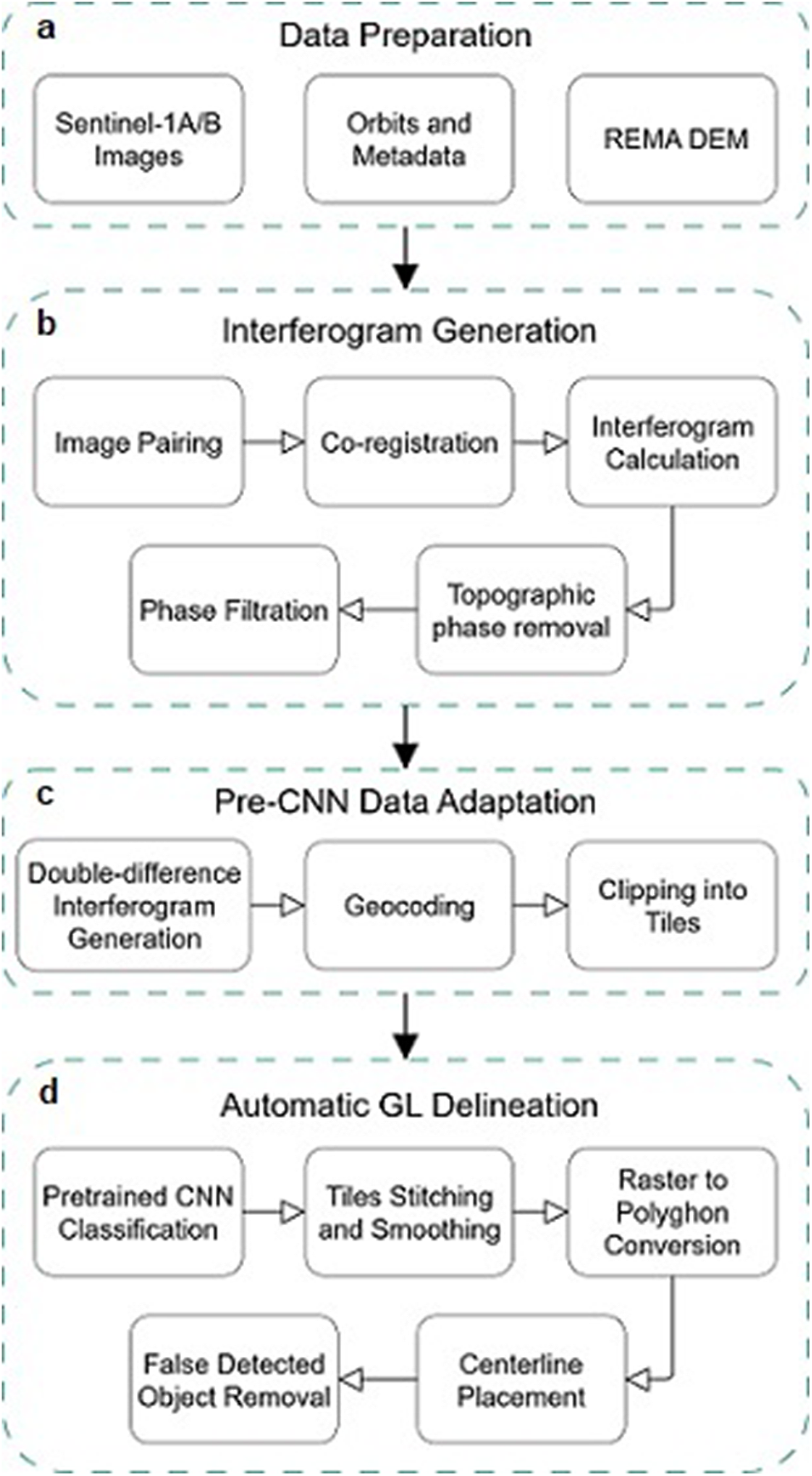
The complete workflow used in this research is illustrated in Fig. 2. The first step is data preparation, in which we gathered all the necessary components for DInSAR calculations (Fig. 2a). Along with the Sentinel-1 images, we collected orbit and metadata for every acquisition, and acquired one digital elevation model (DEM) for the entire area. We formed interferograms by pairing images into a continuous time series (according to the 6 day interval), and by co-registering them subsequently (Fig. 2b). In the next step, we used REMA (Reference Elevation Model of Antarctica) (Howat and others, Reference Howat2022) to extract the topographic phase, and Goldstein’s frequency domain filter (Goldstein and Werner, Reference Goldstein and Werner1998), refined by Baran and others (Reference Baran, Stewart, Kampes, Perski and Lilly2003), to smooth the data. The resulting interferogram consists of a wrapped, filtered phase that indicates surface displacement between two acquisitions. All the calculations were performed with GMTSAR software (Sandwell and others, Reference Sandwell, Mellors, Tong, Wei and Wessel2011).
Data processing workflow: (a) data preparation, (b) interferogram generation, (c) pre-CNN data adaptation and (d) automated GL delineation.

The GL identification is typically performed by experts who manually recognize patterns in the interferograms (Rignot and others, Reference Rignot, Mouginot and Scheuchl2011). Although this GL identification technique is currently considered the most precise (Friedl and others, Reference Friedl, Weiser, Fluhrer and Braun2020), it is also very time consuming. This poses a significant challenge in processing data from a growing number of satellite observations in a reasonable timeframe. In this study, we decided to use a 40-layer convolutional neural network (CNN) developed and trained by Mohajerani and others (Reference Mohajerani, Jeong, Scheuchl, Velicogna, Rignot and Milillo2021) to perform an automatic GL delineation process on 398 four-pass interferograms (252 for path No. 37 and 146 for path No. 49, respectively). CNNs have already been successfully applied not only in object detection (Anantrasirichai and others, Reference Anantrasirichai, Biggs, Albino, Hill and Bull2018; Huang and others, Reference Huang, Luo, Lin, Niu and Liu2020) and classification (Kussul and others, Reference Kussul, Lavreniuk, Skakun and Shelestov2017), but also in the field of glaciology, for example, in the production of sea ice concentration maps (Wang and others, Reference Wang, Scott, Xu and Clausi2016) or the detection of calving zones (Mohajerani and others, Reference Mohajerani, Wood, Velicogna and Rignot2019; Zhang and others, Reference Zhang, Liu and Huang2019). In this case, the CNN was adopted to automatically identify fringe patterns and vectorize the GL, significantly reducing the time needed for obtaining final results. The applicability of this solution has already been confirmed in other GL-detected studies (Ross and others, Reference Ross, Milillo and Dini2024; Tympalski and others, Reference Tympalski, Sompolski, Kopeć and Milczarek2024). According to Mohajerani and others (Reference Mohajerani, Jeong, Scheuchl, Velicogna, Rignot and Milillo2021), this model was trained on 252 manually delineated phase and coherence images of the Getz Ice Shelf. While we apply the same model to a different area, the Orville Coast, the authors demonstrated the model’s high generalization capability and stable performance against independent manual delineations over several Antarctic regions. The resulting mean difference of 232 m and a median of just 101 m demonstrate the network’s ability to correctly predict GL position across different coastal geometries and GZ morphologies. We acknowledge that minor differences in characteristics between the training and study regions may introduce variations in the CNN’s interpretation of interferometric phase patterns. These differences might stem from local topography, ice flow regimes or the angle between the coastline and the satellite line-of-sight. Although fine-tuning might improve local delineation by a few tens of meters, we consider this gain to be marginal in the context of our seasonal dynamics analysis. Therefore, we did not modify the architecture or the pre-trained model, using it exactly as presented by the original authors. Importantly, unlike human interpreters, who may inconsistently classify identical situations, CNN delineates every line consistently.
In the next step of the processing procedure, the data were manually adopted to the mode of CNN functioning (Fig. 2c). We removed the influence of the glacier flow by differentiating subsequent interferograms, that is, by forming their four-pass version. Next, each double-difference interferogram was geocoded to geographical coordinates and cut into 512x512 pixel-size tiles in order to prevent the GPU bottleneck in the subsequent processing. A 10% overlap on each side of every tile helped mitigate edge effects after stitching. The prepared data were then processed by a CNN (Fig. 2d). The network downsamples the data through a series of convolutional layers, each applying a set of filter weights from the pretrained model. As a result, the CNN can detect fine patterns by progressively extracting various features at different levels of abstraction. The upsampling and concatenation functions allowed the features identified by the encoder to be transferred to an upscaled image, which matched the 512x512 pixel-size of the input data. The result is a probability map in which each pixel represents the likelihood of containing the GL. In the next step, full images were rebuilt by stitching the tiles (with the use of a Gaussian filter to reduce edge effects) and vectorized into geospatial polygons. We applied a threshold of 6 km to remove features that were insufficiently large to be reliably recognized as the GL position. In the subsequent delineation process, which was performed with the use of the label_centerlines Python package (Ungar, Reference Ungar2022), the centerline was placed within all vectorized polygons. We also merged the files with the obtained objects into one file corresponding to the acquisition day (last pass for each four-pass interferogram). Note that the resulting objects are obtained with no human intervention, such as user-generated gap-filling or trajectory extrapolation.
The last step in the processing procedure involved manual inspection and filtering of the results provided by the neural network. This process consists of removing clearly irrelevant objects and does not involve their modifications. In our interferograms, each discontinuity of the displacement data (e.g., soil fragments protruding above the ice cover, a boundary between satellite bursts or cracks on the glacial surface) was recognized as a potential GL by the neural network. This problem was common due to poor coherence, which also resulted in missing GL positions. If a part of the glacier was decorrelated in an interferogram, it rendered the detection of the GL position in that area impossible for nearly a month, as one improperly correlated interferogram pair affects two double-difference interferograms (12 days back and forward for a total of 24 days). Although we reduced this effect by increasing the number of observations (we used more than one Sentinel-1 path), some gaps were inevitable. Unfortunately, these problems tend to occur within the GZ, as the melting rate there is relatively high. Consequently, our results needed a thorough review and manual cleaning. Importantly, we could exclude only features distant from the expected GL, and due to the inherent noise and lack of information on the actual GL, it was impossible to distinguish between true and false positive detections of the GL position. Therefore, as no effective methods are yet available for filtering such types of data, our final results may still contain a certain amount of noise.
Dynamics assessment
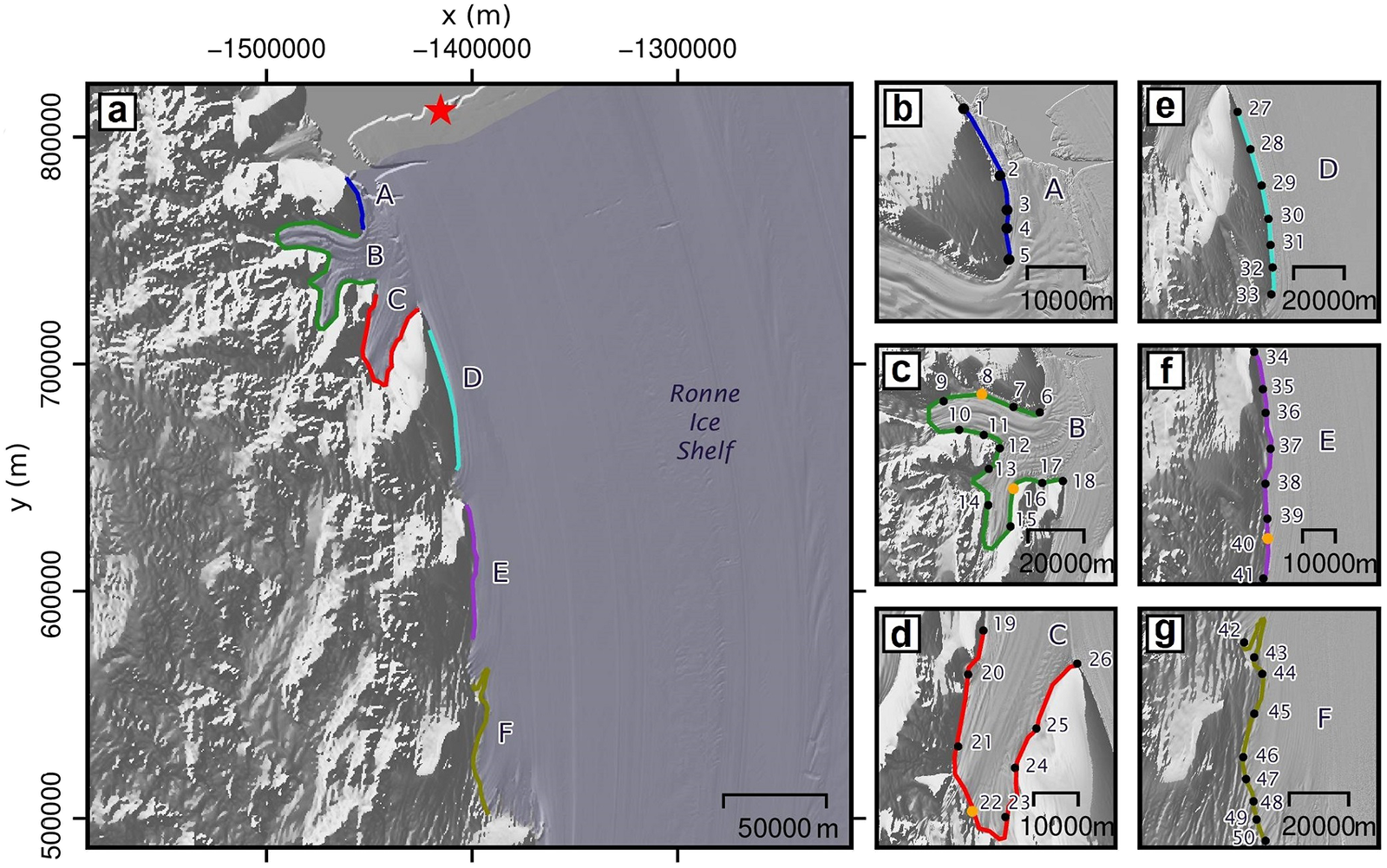
Our processing method produces geocoded vector files with the identified GL positions. In order to enable a deeper analysis, we reduced them to cross-profiles, with each GL represented as a distance to the geometric center (specific for each profile). The Orville Coast is approximately 500 km long and we created 50 profiles, resulting in one profile approximately every 10 km (Fig. 3). However, as the distribution of the results was not spatially consistent, we selected locations where the GL was detected in a larger number of SAR images. The result is thus a non-uniform distribution of cross-sections.
Distribution of the generated profiles and grouping regions. (a) Each colored line and letter label represents a different zone; (b–g) zoom-in view of each zone; black dots indicate the locations of the profiles, while orange dots highlight the locations of the profiles presented in Figure 5. The red star marks the point at which the data on tides were obtained. The map is underlain by a numerical terrain model derived from Bedmap3 (Frémand and others, Reference Frémand2023). Projection: polar stereographic (EPSG:3031).

We divided the study area into six zones to address potential gaps caused by poor coherence or missing Sentinel-1 acquisitions. The segmentation into zones was also aimed at mitigating the influence of anomalies resulting from local topography changes, and thus reducing the number of outliers. We grouped several profiles, with the assumption that the glacier behaves as a single body in terms of GL migration. Zones A, D, E and F have almost linear GL, likely because they are located perpendicular to the main flow of the glacier. Moreover, zones D–F are separated only by small ocean intrusions, which discontinue the GL, and thus justify our decision to classify these zones as separate segments. The classification is also motivated by the Sentinel-1 path coverage, as the ascending path (No. 49) ends in the vicinity of the intrusion between zones E and F, and provides limited results for zone D. On the other hand, the GL is curved in zones B and C, which are both located within the bay, where the ocean penetrates deeper beneath the glacier. In this area, we expect the velocities and ice masses to have a smaller impact on the erosion of the seabed, allowing other phenomena (e.g., tides and water intrusion) to have a greater influence on the GL migration. Although there are three valleys visible in the bay, we define just two zones here: one for the wider southernmost valley, and another for the two narrower valleys.
We investigated the GL migration mechanisms by examining two key aspects: the response of the glacier to tidal changes and the temporal movements within the GZ. In both cases, it is important to identify the migration extremes. We examined their distribution over the study period and across the defined zones, determining the width of the GZ based on the observed GL positions. However, our observations are limited by the temporal resolution of the available data and by their quality, as decorrelations within the GZ can prevent successful GL detection. Therefore, the actual migration might vary from the extremes we were able to identify. Subsequently, the observed migration was compared with the theoretical values, calculated from the HE equation:
 \begin{equation}
\begin{aligned}
GZ_{HE} = \Delta h_t \cdot \left( \beta + \frac{\rho_i}{\rho_w} \cdot (\alpha - \beta) \right)^{-1},
\end{aligned}
\end{equation}
\begin{equation}
\begin{aligned}
GZ_{HE} = \Delta h_t \cdot \left( \beta + \frac{\rho_i}{\rho_w} \cdot (\alpha - \beta) \right)^{-1},
\end{aligned}
\end{equation}where  $\Delta h_t$ is the maximum predicted tidal difference observed during the period, $\rho_i$ = 917 kg m $^{\text{-}3}$ and $\rho_w$ = 1027 kg m $^{\text{-}3}$ represent the densities of ice and seawater, respectively, and $\beta$ and $\alpha$ are the bedrock and ice surface slopes, respectively. The slope values were derived from Bedmap version 3 (Frémand and others, Reference Frémand2023) by averaging the slopes within a 4 km-wide buffer for each zone. A perfect range would be identical to the GZ width, but as the data resolution is 500 $\times$ 500 m, we decided to expand the area to at least eight pixels. This adjustment not only helped to avoid potential local anomalies but also reduced the uncertainty to a level below 0.1 degree. The process was performed separately for both the bedrock and the surface slopes. We compare these slope values with the observed GZ width in every zone to assess their influence on GL migration. The data on tides were predicted using the CATS2008 model (Padman and others, Reference Padman, Erofeeva and Fricker2008; Howard and others, Reference Howard, Erofeeva and Padman2019), which provides tide-height information with an accuracy of 5 cm (Glaude and others, Reference Glaude2020). These data were acquired at a point ( $-$1 415 278.74, 811 497.37; EPSG:3031) located nearly 50 km from the GZ, at the approximate latitude of our first profile (Fig. 3a). This strategic placement, just before the glacier terminus, avoids the uncertainty of tide value prediction under the glacier cover. Additionally, we applied the inverse barometer effect (IBE) correction to tides, based on sea level pressure provided by the European Center for Medium-Range Weather Forecasts (Hersbach and others, Reference Hersbach2020). These data reduce the influence of the isostatic response of the ocean to changes in the atmospheric pressure (Padman and others, Reference Padman, King, Goring, Corr and Coleman2003), and thus help obtain more accurate tide-height values. As we are working with four-pass interferograms, which represent a combined signal from four different acquisitions, we also accordingly determine the differential tide:
 \begin{equation}
\begin{aligned}
DD_{tide} = (t_B - t_A) - (t_D - t_C),
\end{aligned}
\end{equation}
\begin{equation}
\begin{aligned}
DD_{tide} = (t_B - t_A) - (t_D - t_C),
\end{aligned}
\end{equation}where 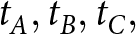 $t_A, t_B, t_C,$ and $t_D$ correspond to the IBE-corrected tide-height values at the exact date and time of the four SAR measurements used to generate each four-pass interferogram. These combined operations ensure a better alignment between the tide height and the displacement observed in the four-pass interferogram. Finally, we conducted a correlation analysis to investigate the relationship between displacement values, tidal variations and GL migration.
Validation
The relatively small number of studies on the Orville Coast limits the available datasets that can be used to validate our results. We found two such potentially useful datasets: the MEaSUREs Grounding Zone of the Antarctic Ice Sheet, v2 (Rignot and others, Reference Rignot, Mouginot and Scheuchl2016) and the Antarctic Ice Sheet Climate Change Initiative (AIS CCI) v2.0 (Floricioiu and others, Reference Floricioiu, Krieger, Chowdhury and Bässler2021). Unfortunately, the MEaSUREs dataset is unavailable for the specific period of our analysis and the study area. The AIS CCI dataset consists of several records per year, and each record includes metadata with the exact acquisition date. The data span a period partially overlapping with our studies for the years 2017–20. However, the data are not available for the entire Antarctic region. The only three records that cover our study area in the Orville Coast are from the year 2020, and as our data for these particular days are incomplete, the spatial comparison proved impossible. Since we found no suitable vector dataset, we decided to validate our data against an outline of the grounded ice mask derived from Bedmap version 3 (Frémand and others, Reference Frémand2023). Bedmap3 provides a comprehensive, continent-wide Ice/Ocean/Land Mask used to delineate grounded ice areas. Mapping the GL is problematic due to the disparate nature of various source data (varying spatial scales, time periods and sampling frequencies) and the dynamic behavior of the GL (oscillating with tidal cycles or migrating over time). Bedmap3 addresses the above problems by integrating diverse remote sensing data from radio-echo sounding (RES), satellite altimetry (RTLA), interferometric synthetic aperture radar (InSAR) and optical imagery into a harmonized, uniform 500 m grid. The use of multiple data sources ensures resilience to systematic errors. Notably, the core layers of Bedmap3 do not rely on ice sheet models or inversions of bed topography. Therefore, the Bedmap3 validation dataset provides an independent and relatively robust validation dataset. Our validation process employed the PoLiS metric (Avbelj and others, Reference Avbelj, Müller and Bamler2015), which is a distance function designed to quantify the dissimilarity between two polygons or line segments, as demonstrated in Heidler and others (Reference Heidler, Mou, Loebel, Scheinert, Lefèvre and Zhu2023). PoLiS calculates the average of the minimum Euclidean distances from each vertex of one polyline/polygon to the boundary (edges and vertices) of the adjacent polygon and satisfies such criteria as positive definiteness, symmetry and the triangle inequality. This process is bidirectional, and its results are averaged and normalized by the number of vertices in each respective polyline/polygon. This approach allows for the geometric shape of the objects, overcomes the limitations of point-set-based measures (e.g., Hausdorff and Chamfer distances) and offers approximately linear response to small transformations. The Bedmap3-derived polyline was clipped to a 4.5 km-wide buffer around each line of our dataset, which was necessary as significant length differences affect the overall metric value.
Results
Based on 398 double-difference interferograms, the CNN identified over 40 000 objects as potential GL positions. Most of these objects were located far from the GZ and were immediately removed, according to the procedure described in the methodology section. The CNN identifies these false positives because their phase discontinuities are similar to the signal of a true GL position, although such cases are characterized by a much smaller spatial extent. The manual filtering reduced the dataset by 62%, leaving 15 535 true GL objects. An average of 40 lines per image presents how scattered and discontinuous the results were.
The validation of the obtained GL positions against the Bedmap3-derived GL resulted in mean and median PoLiS values of 1300 and 811 m, respectively. Considering that the grounded ice raster mask from Bedmap has a spatial resolution of 500 m and is based on measurements taken between 1990 and 2023, our results are sufficiently close to the baseline to call them reliable. Additionally, the fact that we compare a single, static line to multiple migrating lines may be a factor contributing to the larger PoLiS values. Note that other remote sensing methods exhibit uncertainties reaching approximately 1000 m (Friedl and others, Reference Friedl, Weiser, Fluhrer and Braun2020). Given the above, we believe our results to be a valid representation of the GL position.
To estimate the agreement between the results obtained from the two acquisition paths, we performed a statistical comparison of the derived GL positions. The analysis involved determining the percentage of points from one path that had a corresponding spatial-temporal neighbor in the other path. The temporal search window of 15 days was used to establish a temporal tolerance for matching non-synchronous observations and to account for cases where a direct neighbor from either path was missing. The maximum spatial tolerance was initially set to 100 m, as a compromise between statistical rigor and accounting for potential GL migration relative to tidal variations. The statistic returned a value of 44.58%, indicating that nearly every second point from one path has a similar observation in the other path. When the search window was increased to 200 m, the percentage of agreement rose to 67.26%, meaning that only about one-third of points lacked a corresponding match between paths. We note that the overall statistic may be slightly underestimated, because the temporal window search does not guarantee the existence of data, as for some acquisition dates, the GL could not be identified at all due to missing data or poor coherence. Nonetheless, we assess this statistical result as a high level of alignment, which demonstrates that the two acquisition geometries provide valid information about GL migration and can be treated as equivalent for the purposes of this study.
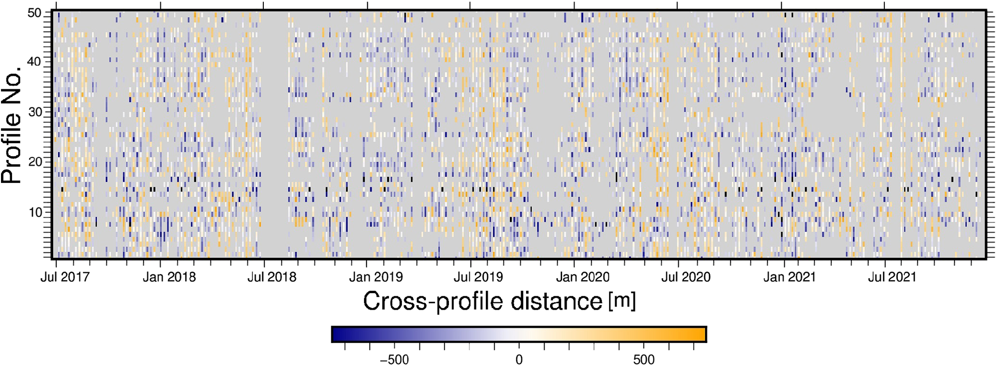
In order to further analyze the results, we developed a heatmap (Fig. 4) for the descending path No. 37. By gathering all the measurements on a single plot, we were able to evaluate both the quality of the outcome and of the glacier behavior. To reduce the figure size and improve readability, the time axis consists only of dates with expected Sentinel-1 acquisitions.
Results of GL positions from descending path No. 37 over the studied period, along defined cross-profiles. The blue and yellow colors represent retreat and advance, respectively, indicating the GL position relative to the midpoint of each individual profile. The gray color represents days with no measurements.

The predominance of gray in the heatmap showcases the extent of missing data. This is primarily due to missing Sentinel-1 acquisitions (i.e., September 2017, July 2018, December 2018, March 2019, June 2020 and July 2021), which results in no observations on any of the profiles on a total of 24 dates. Another contributing factor is the greater melting during the summer months, which leads to increased decorrelation. Of the 6386 missing data points, 65% occur in the summer season. Despite these complications, a recurring seasonal pattern can be observed: positive values (yellow, i.e., advance) tend to occur during the winter season (59.34% of all observations in this season), and negative values (blue, i.e., retreat) are generally observed in summer (57.29% of all observations in this season). This temporal pattern is of significance in our further investigations.
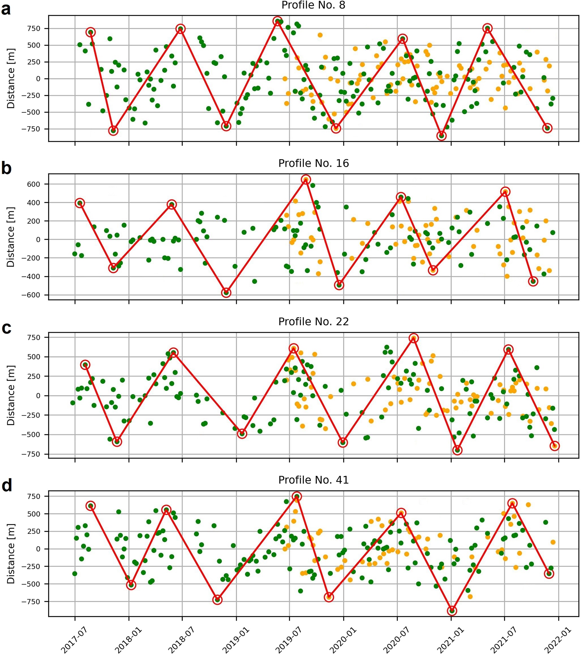
We proceeded with the identification of yearly migration extremes on each profile. In Fig. 5, we show four profiles that reflect the distribution of the values within the entire set. Negative values indicate inland retreat, and positive values indicate the advance of the GL towards the ocean. The different colors in the figure represent data derived from the different Sentinel-1 paths.
GL migration identified on selected profiles, represented as distances for individual dates. Green and orange dots indicate the measurements from a particular Sentinel-1 path, No. 37 and No. 49, respectively. Red circles mark the minimum and maximum migration ranges within a year, with the red line illustrating the temporal pattern.

The minimum and maximum migration ranges (marked red) can be identified despite the significant noise. As a result, the GZ width can be assessed to range from 1000 to 1500 m. The positions of the migration extremes suggest that they tend to occur in the middle and at the end of the calendar year, confirming the observation in Fig. 4. The red lines connecting the identified extremes illustrate the temporal pattern. While we explored several alternative fitting approaches, the noise in our data obliged us to define the seasonal trend based solely on the maximum and minimum extent of the observed migration. Nevertheless, the lines visually highlight the overall year-to-year changes and how other data points cluster around them. It further supports our conclusion regarding seasonality in the migration.
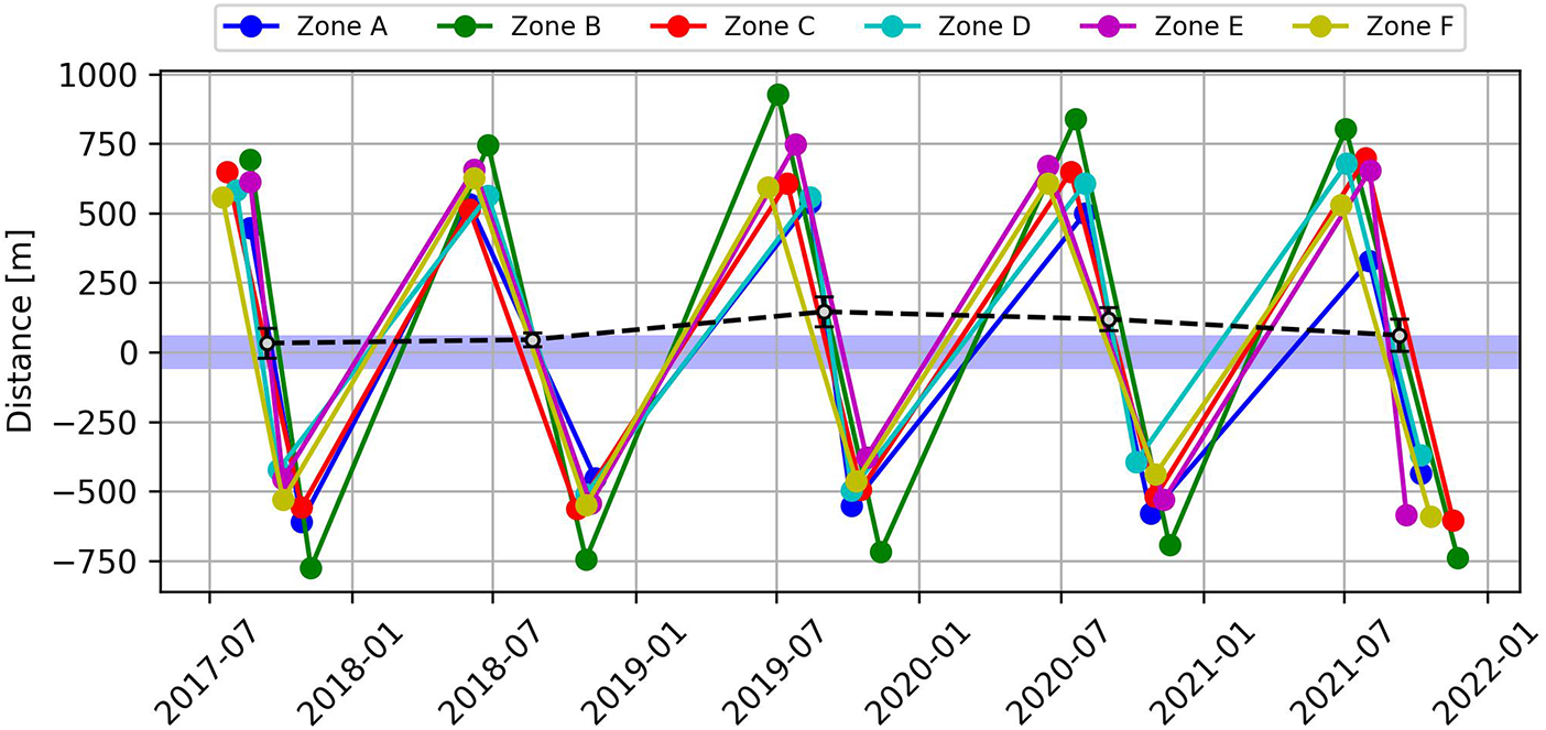
The next step in our procedure was to identify the migration ranges in the stacked profiles within each zone (A–F), following an approach similar to that used for a single profile. To improve the clarity of the graph (Fig. 6), we excluded the individual data points and presented only the overall annual extreme values identified for each zone. Based on these extrema, we determined the annual GL equilibrium positions (black circles). The date of each point was calculated as the midpoint between the occurrences of the extrema within the given year. The mean GL position and its uncertainty were then derived from the equilibrium points across all zones for that year. The dashed black line connecting the equilibrium positions illustrates the overall year-to-year variability. We also show the mean maximum theoretical migration range (144 m), derived from the HE equation (1).
GL migration extremes for different zones. The colored points and continuous lines indicate annual migration extremes and seasonality for each zone (color-coded similarly to Fig. 3). The black circles present annual average GL positions, with vertical black bars indicating data variance. The shaded blue zone around the value zero shows theoretical maximum ranges of migration derived from the HE equation.

The migration extremes appear to be very similar across different zones. They are consistent in terms not only of the period of occurrence but also of the values reached. This observation confirms the glacier behavior as a single body and the occurrence of seasonal movements. We identified the GZ width of the straight shoreline segments of the Orville Coast to be approximately 1050 m (zones A, D–F). For zones B and C located within the bay, mean migration ranges reach 1550 and 1200 m, respectively. While zone B exhibits a considerably wider migration, the GZ width in zone C is comparable to the values observed in the straight shoreline areas. The line connecting the annual averages of GL positions shows subtle interannual oscillations, with the slight 2019 advance as the most prominent example. However, the associated vertical error bars indicate that these variations are within the uncertainty of the data. Since the error margins overlap between years, these observed year-to-year changes are not statistically significant and cannot lead to any definitive statements about observed advance or retreat. The results generally seem to confirm the relatively stable behavior of the GZ in this area, without notable shifts or deviations observed during the investigation period.
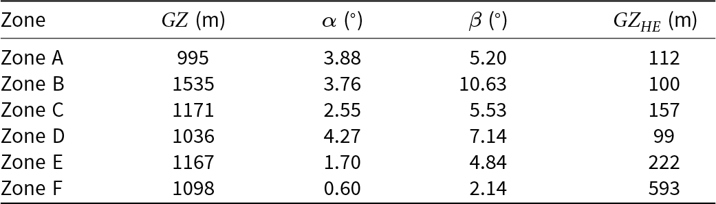
With the migration extremes identified, it was possible to compare the observed GZ width with the theoretical range ( $GZ_{HE}$) derived from the HE equation (1). The results are presented in Table 2. For each zone, the observed GZ width was calculated as the average of annual GZ widths, and each annual width was determined as the difference between the minimum and maximum migration in a particular year. The theoretical GZ width is calculated for each zone based on the measured ice surface ( $\alpha$) and bedrock ( $\beta$) slopes in that zone. The maximum tidal difference ( $\Delta h_t$) is a single value used for all zones, derived from the absolute maximum (158.6 cm) and minimum (-67.1 cm) predicted tide values observed during the entire investigated period.
Observed ( $GZ$) and theoretical ( $GZ_{HE}$) GZ widths across the zones.
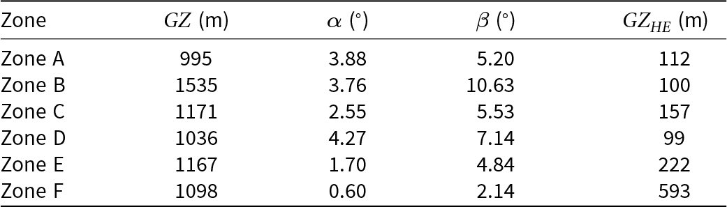
As evident from the data, the observed migration is significantly greater than the migration calculated from the HE equation. The theoretical values are relatively low, with the values between 100 and 200 m in most cases. The only exception is zone F, where the theoretical migration reaches up to 593 m due to low ice surface and bedrock slopes. Here, the calculated value is only two times lower than the measured value. For the remaining zones, the calculated values are 5–10 times lower, with the migration for zone B being 15 times lower than its observed value. Notably, the zone with the largest observed migration (zone B) has one of the lowest theoretical values.
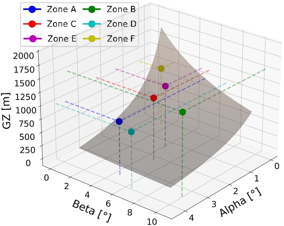
To perform a deeper analysis of the relationship between the ice surface slope ( $\alpha$), bedrock slope ( $\beta$) and observed GZ width (GZ), we created a plot (Fig. 7) that allows a direct comparison between these three variables. We also included a theoretical surface, which illustrates the inverse relationship derived from the HE equation.
The influence of local topography on the GZ width observed across different zones. The colored points indicate the observed relationship between the ice surface slope ( $\alpha$), bedrock slope ( $\beta$) and observed GZ width (GZ) for each zone. The gray surface represents the theoretical dependency between these three variables.

The figure confirms that the observed GZ width significantly exceeds the maximum migration range derived from the HE equation, as the observed GZ value for each zone lies above the theoretical surface, to which zone F is the closest one. The plot illustrates that lower surface and bedrock slopes lead to a greater maximum theoretical migration width. Despite this agreement with the theory, we cannot establish a clear correlation between these three variables. This suggests that the migration within the GZ width is driven by dynamic factors beyond the static topographic parameters.
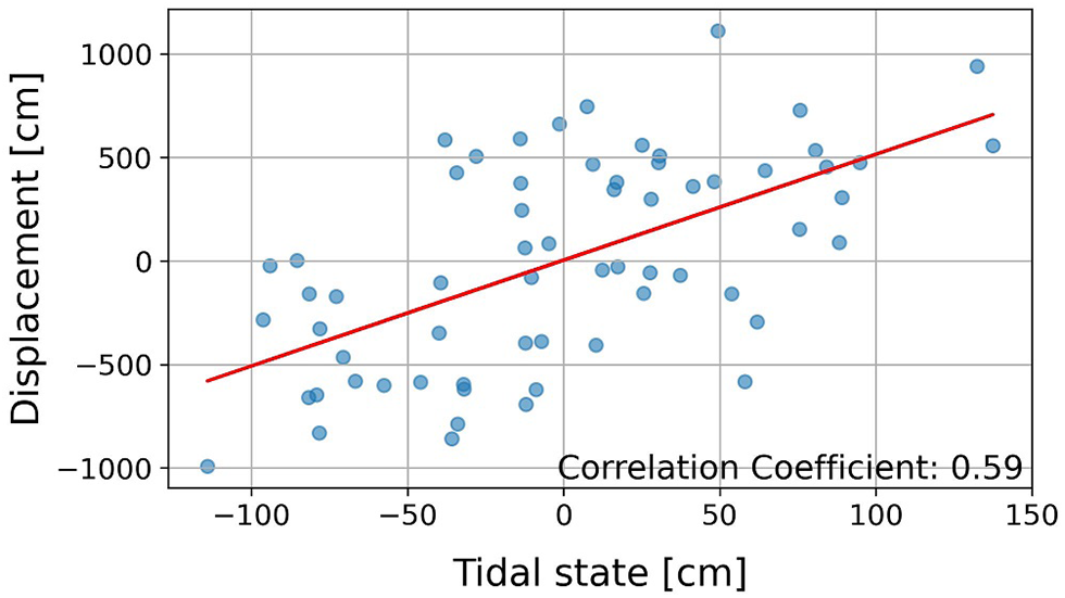
Finally, we utilized the data on the tides to verify the quality of the results and assess their influence on the glacier behavior. The displacement values in the calculated four-pass interferograms showed high similarity with the predicted differential tide values, as presented in Fig. 8, and provided an overall correlation coefficient of 0.59. Converting the phase difference interferogram into motion displacements requires phase unwrapping, which is time-consuming when the data coherence is insufficient. Therefore, we performed this process only on every third interferogram.
Predicted differential tide value versus displacement range on calculated four-pass interferograms, with the regression line in red.

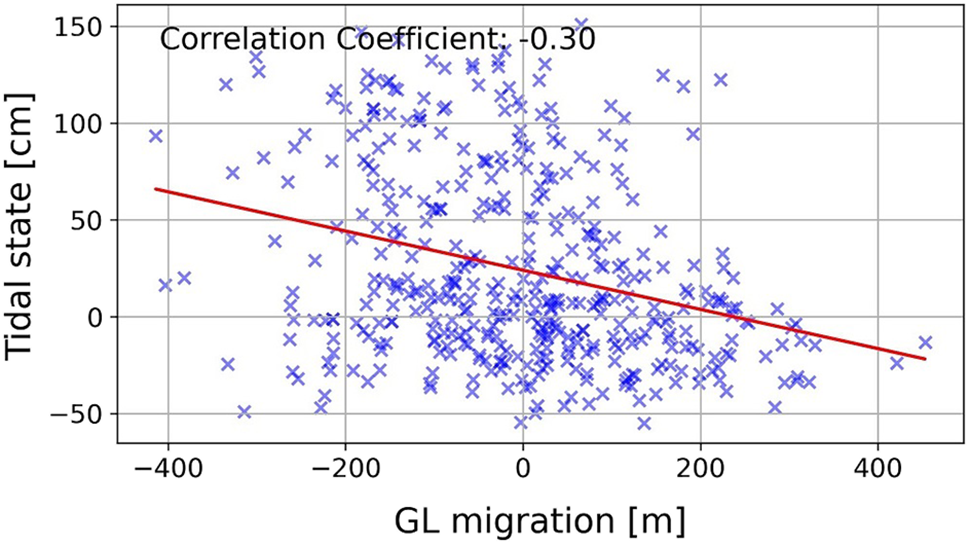
We compared predicted differential tide values with GL positions accordingly (Fig. 9). Here, they are defined as the mean of GL positions detected across all profiles for a given day. The resulting correlation coefficient was -0.30. The negative correlation confirms the expected relationship: as tidal levels increase, the GL generally retreats.
Predicted differential tide value versus daily-averaged GL positions, with the regression line in red.

To ensure the reliability of the results, we performed a statistical significance test for Pearson correlation, which yielded t-statistic values of 5.28 and 4.84 for tides versus displacements ( $N$=64) and for tides versus the GL position ( $N$=292), respectively. As both of these values exceed the critical value of 1.97 (for a two-tailed test at $\alpha$=0.05), our results indicate a statistically significant relationship. The general conclusion is that although the influence of tides on GL migration is detectable, they are not the dominant factor driving these changes.
Discussion
This study confirms the applicability of double-difference interferometry (Rignot and others, Reference Rignot, Mouginot and Scheuchl2011) and machine learning algorithms (Mohajerani and others, Reference Mohajerani, Jeong, Scheuchl, Velicogna, Rignot and Milillo2021) in GL delineation and supports further development of the presented methodology. The use of satellite data in combination with automatic data-processing algorithms provides improved spatial and temporal coverage and allows results to be obtained at more regular time intervals, as frequent as 1 week. The presented methodology is season-, sunlight- and weather-independent (Nagler and others, Reference Nagler, Rott, Hetzenecker, Wuite and Potin2015). Its main advantage is the fact that GL is delineated with a precision down to approximately 100 m in the DInSAR method (Rignot and others, Reference Rignot, Mouginot and Scheuchl2011; Rosier and others, Reference Rosier, Marsh, Rack, Gudmundsson, Wild and Ryan2017), while other remote sensing methodologies are limited to accuracies around 1000 m (Joughin and others, Reference Joughin, Shean, Smith and Dutrieux2016; Dawson and Bamber, Reference Dawson and Bamber2017; Friedl and others, Reference Friedl, Weiser, Fluhrer and Braun2020). The alignment between the two different Sentinel-1 paths of 67.26% confirmed that the results obtained from different flight directions are consistent. Our observations indicate that interferograms from the ascending path No. 49 have slightly less noise, which suggests that this acquisition geometry better captured the signal of interest and provided more precise observations. This may be caused by the fact that the coastline in this area is nearly parallel to the direction of the satellite’s line of sight, but this phenomenon should be verified in future research. Despite the above, we can confirm that results from two different paths can be viewed as equivalent to data from one source, also in the case of ice-sheet measurements.
The raw results produced with the automatic delineation process contain significant noise, with less than 40% of the identified objects being true positive detections. The main difficulty here is maintaining coherence, especially within the displacement occurrence just above the GZ. In GMTSAR, the interferograms are filtered with Goldstein’s frequency domain filter (Goldstein and Werner, Reference Goldstein and Werner1998), refined by Baran and others (Reference Baran, Stewart, Kampes, Perski and Lilly2003). Some filters, for example, the InSAR-BM3D filter (Sica and others, Reference Sica, Cozzolino, Zhu and Poggi2018) or filters based on deep learning (Murdaca and others, Reference Murdaca, Rucci and Prati2022) may be able to preserve the phase structures more precisely. Their application could improve the quality of the interferogram and thus facilitate the GL detection process. Further improvements may involve the ability of current machine learning algorithms to work with discontinuous interferometric data. These algorithms consistently mark a GL at each termination of the fringe pattern, even if induced by decorrelation or noise. This behavior may be the most disruptive factor to our time series, as such false positives are impossible to be distinguished from true positives. Better identification of the interrupted phase can significantly improve the potential of this method for seasonality detection in GL migration.
Despite the noise in the data, we successfully identified the GL extremes (Figs 5 and 6), and thus achieved our main research goal. Our results confirm that the GL migration is similar in time and range throughout the glacier. The line connecting the annual averages of GL positions shows subtle interannual oscillations. However, the analysis of the associated vertical error bars demonstrates that these variations are within the uncertainty of the data. Therefore, we cannot draw any definitive statements about advance or retreat of the GL. In general, the results confirm the stable behavior of the GZ in this area. Our research also included the analysis of the influence of local topography on the GZ width (Fig. 7). Despite a clear relationship between ice surface and bedrock slopes and maximum theoretical migration width, we cannot establish a correlation between local topography and observed GZ from our data. This suggests that the migration within the GZ width is driven by dynamic factors beyond the static topographic parameters.
Our investigations also included the comparison of predicted from the CATS2008 model differential tide values with the ice shelf displacement (Fig. 8) and with the GL position (Fig. 9). The displacement values in the calculated four-pass interferograms showed high similarity with the predicted differential tide values, which confirms the ice shelf’s response to ongoing tidal forcing. Notably, while the tidal data are aligned temporally with satellite acquisition, the ice masses may not respond immediately to the uplift caused by tides. The low correlation with the GL migration may suggest that tides are not the main factor contributing to GL movement, even with clear consistency between the tide values and the range of the displacements on the interferograms. These results corroborate findings from recent studies (Chen and others, Reference Chen, Rignot, Scheuchl and Ehrenfeucht2023; Li and others, Reference Li, Dawson, Chuter and Bamber2023). The analysis of our time series indicates that these influences need to be investigated from a different perspective. The identified seasonality suggests that the long-range migrations (on the order of hundreds of meters within a year) may be due to other dominant factors, such as atmospheric and ocean temperature changes. However, the influence of tides may be observed by analyzing more local (e.g., week-to-week) changes in the GL position. We assume that the correlation between GL migrations and tide height will be more detectable after the time series are decoupled from seasonality.
The disparity visible in Fig. 9 is also interesting. Intuitively, the values should be present only in the upper-left and lower-right corners, confirming the assumption that the glacier retreats at high tides and advances at low tides. This logic is supported by the observation that the data points are almost absent in the upper-right corner. However, the situation is different on the opposite side, where the GL remains negative even at a negative tidal state. This fact suggests that despite the lower tidal state, the GL remains retreated further inland rather than advancing toward the ocean. Similar findings have been documented in other studies (Chen and others, Reference Chen, Rignot, Scheuchl and Ehrenfeucht2023; Freer and others, Reference Freer, Marsh, Hogg, Fricker and Padman2023; Antropova and others, Reference Antropova, Mueller, Samsonov, Komarov, Bonneau and Crawford2024). The evidence is also found in Fig. 6, in which the extremes do not occur within a 6 month interval. The annual maximum advances occur only during the austral winter, as June, July and August account for 10, 11 and 9 observations, respectively. In contrast, the annual minimum positions are strongly clustered in October and November, which account for 20 and 8 observations, respectively. This indicates that the retreat phase, typically lasting 3–4 months, is shorter in duration than the advance phase, typically lasting 8–9 months. The annual minimum is therefore observed almost immediately after the previous annual maximum. While the exact cause behind these changes remains unclear, the observed longer duration of the advance phase could potentially be explained by the mechanism proposed by Rignot and others (Reference Rignot, Ciracì, Scheuchl, Tolpekin, Wollersheim and Dow2024), which indicates that the pressure causes water to remain under the glacier for extended periods, consequently slowing the advance process. Although a more detailed analysis of the physical mechanisms driving this disparity is beyond the scope of the present work, we strongly encourage further investigation of this phenomenon by the scientific community.
The four above publications also mention that the actual width of the GZ seems to be significantly greater than expected. Our research results support these findings (Table 2). The observed width of the GZ is 5–10 times greater than the value calculated with the HE equation, and in the case of zone B, the value is 15 times greater. The exception is zone F, where the observed migration is only two times larger than the theoretical migration, which is due to the low ice surface and bedrock slopes in this zone. The discrepancy between the observed and maximum theoretical GZ width is primarily due to the significant underestimation of the theoretical value, and demonstrates the need to develop new methods and models for estimating the migration range.
Another important matter concerns results reproduction. There are several elements in the CNN learning process that can lead to slightly different final weight values and, consequently, slightly different results. First, neural networks may focus on different features of the input data depending on the order of the input images. This variability is mitigated to some extent by using a large number of inputs in order to ensure generalization. A common practice in training neural networks is to randomly exclude data from the training set to form a validation set, which is used to monitor the network’s performance data and to prevent overfitting. Second, the initialization of weights can be random or follow a specific probability distribution. This step reduces the risk of CNN converging to a local minimum during the weights optimization process, known as gradient descent. Third, dropout layers are often used to prevent overfitting by randomly excluding a portion of inputs from the previous layer, before passing them to the next layer. The three techniques cause the final set of network weights to vary after each training process, producing slightly different results. This variability is an integral part of the training phase itself, but it does not affect the reproducibility when using a fixed, pre-trained model. For this reason, we are not performing our own training and instead utilize an already validated model, thereby ensuring that the results can be reproduced.
Conclusions
This paper presents the results of the first research dedicated to the GL position on the Orville Coast. It also offers a new approach to the analysis of GL migration from a longer-term (4.5 year) perspective and with a temporal resolution of less than 1 week. The combination of the double-difference interferogram method with a dedicated neural network serves as a useful tool in detecting GL positions. Despite challenges such as maintaining coherence and controlling data noise, we were able to identify the migration extremes and thus detect the seasonality of the GL movements. The migration in the zones comprising a straight shoreline was found to be more stable than the movement within the bay, as the narrow-type valley seems to increase the influence of the tides, which increases the migration range. The observed GZ width is significantly greater than the maximum extent of theoretical migration, calculated from the HE equation. The migration is also less dependent on the tidal state, even when the displacement value on the interferogram is consistent with the predicted differential tide value. We also show the feasibility of employing two Sentinel-1 tracks with different flight directions. Their use leads to a more consistent time series and the filling of the missing data gaps, as well as a reduction in time intervals between individual results to less than 6 days. This method can thus provide grounds for further studies of glacier behavior around the GZ.
Our results represent a new approach to seasonality and trend assessment in GL migration. We believe that our findings have the potential to help detect patterns in glacier behavior and identify the causes of changes occurring in the GZ. We hope that our results will also contribute to the exploration of the causes for glacier retreat and, in the longer perspective, to providing insights for developing effective ways of limiting glacier retreat. This might be the crucial factor mitigating the mass loss of glaciers, which is especially important in times of ongoing major climate change.
Further research is recommended to focus on improving machine learning algorithms, in order to achieve more effective control of the discontinuities in the displacements on interferograms, to generate a higher percentage of true GLs. The performance of the proposed methodology could also be significantly improved with further developments of the DInSAR method for the purpose of GL delineation, for example, by improving phase smoothing and filtering algorithms. Advancements in statistical analysis techniques applied to the time series of GL positions are also very important, as they could not only clear noise from the data, but also fit the seasonality function and filter it out from the time series. Further investigations may also focus on the use of paths with a different flight direction and their sensitivity to ice shelf motion. Although this study confirms the consistency of results obtained from different flight directions, employing a specific trajectory could potentially lead to higher-quality results (e.g., less noise on four-pass interferograms), depending on the characteristics of the ice shelf. Finally, as the study confirms a weak correlation between tidal changes and GL positions, the main factors influencing GL migration require further research. We strongly encourage future research into the processes driving GL migration and the presence of deep-water intrusions beneath the glacier, even during periods of low tide.
Data availability statement
The raw radar data used in this study are available open source from the Alaska Satellite Facility Data Search Vertex platform at https://search.asf.alaska.edu.
Acknowledgements
The authors thank the Editors and two anonymous reviewers for their constructive feedback, which improved the content and clarity of the manuscript. This research was funded by Wrocław University of Science and Technology within the Academia Professorum Iuniorum programme.







 Open access

