1 INTRODUCTION
The counterplay between observation and theory, the constant iterative process by which models interpret data, and data in turn enhances and improves models, is central to the exercise of modern astrophysics. Observations by their very nature are never entirely complete, nor infinitely precise; it is impossible to fully understand the interior of a star or the properties of an unresolved stellar population from observational data alone. Instead, observations are compared to theory and a prescription developed which best fits both the data and our understanding of the physical laws and processes governing the system under observation. In making the comparison, theoretical or numerical models may be discounted or modified, while they, in turn, suggest further observations that may help distinguish between competing interpretations.
Increasingly important for interpreting observations of populations (rather than individual instances) of astrophysical objects is the concept of stellar population and spectral synthesis. Stellar population synthesis combines either theoretical or empirical models of individual stars according to some mass and age distribution, to predict the ratios of different stellar subtypes, the frequencies of transient events, or the probability of recovering an unusual object as a function of luminosity, density, or evolutionary state. Spectral synthesis combines these stellar population models with stellar atmosphere models, and sometimes with non-stellar components such as dust and nebular gas, to predict the colours, line strengths, and other observational properties of an observed population (see Conroy Reference Conroy2013, for a recent review).
It is important not to underestimate the assumptions that go into these models and the uncertainties associated with them. Population synthesis models have been in existence for several decades, with popular examples including starburst99 (Leitherer et al. Reference Leitherer1999) and, for galaxy evolution studies, the galaxev models of Bruzual & Charlot (Reference Bruzual and Charlot2003). These codes are still in active development and continue to add to their initial model grids, with v7.0 of Starburst99 recently supporting stellar models from the Geneva group which incorporate rotational mixing effects (Leitherer et al. Reference Leitherer, Ekström, Meynet, Schaerer, Agienko and Levesque2014). However, work in recent years has demonstrated that there is still much to improve in population synthesis (Leitherer & Ekström Reference Leitherer, Ekström, Tuffs and Popescu2012; Conroy Reference Conroy2013, and references therein), refining models to address a number of physical processes that are currently not included. Stellar atmosphere models are being revisited to better match the spectra of observed stars across a broad range of metallicities and evolutionary states. The underlying stellar evolution models are also undergoing an unprecedented increase in accuracy (see e.g. Langer Reference Langer2012).
Perhaps, most importantly, there is an increasing recognition in the community that it is impossible to ignore the effects of stellar multiplicity when modelling the evolution and observable properties of young stellar populations, whether or not these are resolved. Sana et al. (Reference Sana2012) estimated that 70% of massive stars will exchange mass with a binary companion, influencing their structure and evolution. While the exact fraction likely varies with environment, stellar type, mass ratio and metallicity, recent estimates of the binary, or multiple fraction from both the Milky Way (Duchêne & Kraus Reference Duchêne and Kraus2013; Yuan et al. Reference Yuan, Liu, Xiang, Huang, Chen, Wu and Zhang2015; Sheikhi et al. Reference Sheikhi, Hasheminia, Khalaj, Haghi, Zonoozi and Baumgardt2016) and the Magellanic Clouds (e.g. Li, de Grijs, & Deng Reference Li, de Grijs and Deng2013; Sana et al. Reference Sana2014) suggest that field F, G, K stars may have an observed binary fraction of 20–40%, while that for O and B type stars may reach 100%.
There are several codes and groups that study and account for interacting binaries in population synthesis (e.g. Belczynski et al. Reference Belczynski, Kalogera, Rasio, Taam, Zezas, Bulik, Maccarone and Ivanova2008; De Donder & Vanbeveren Reference De Donder and Vanbeveren2004; Hurley, Tout, & Pols Reference Hurley, Tout and Pols2002; Izzard et al. Reference Izzard, Glebbeek, Stancliffe and Pols2009; Lipunov et al. Reference Lipunov, Postnov, Prokhorov and Bogomazov2009; Toonen & Nelemans Reference Toonen and Nelemans2013; Tutukov & Yungelson Reference Tutukov and Yungelson1996; Willems & Kolb Reference Willems and Kolb2004). However, spectral synthesis including interacting binary stars has not received the same amount of attention. For a considerable time, only two groups have worked on predicting the spectral appearance of populations of massive stars when interacting binaries are included. These are the Brussels group (e.g. van Bever & Vanbeveren Reference van Bever and Vanbeveren1998; Van Bever et al. Reference Van Bever, Belkus, Vanbeveren and Van Rensbergen1999; Van Bever & Vanbeveren Reference Van Bever and Vanbeveren2000, Reference Van Bever and Vanbeveren2003; Belkus et al. Reference Belkus, Van Bever, Vanbeveren and van Rensbergen2003) and the Yunnan group (e.g. Zhang, Li, & Han Reference Zhang, Li and Han2005; Li & Han Reference Li and Han2008; Han, Podsiadlowski, & Lynas-Gray Reference Han, Podsiadlowski and Lynas-Gray2007; Han & Han Reference Han and Han2014; Zhang et al. Reference Zhang, Li, Cheng, Wang, Kang, Zhuang and Han2015). The predictions of these codes are similar: binary interactions lead to a ‘bluer’ stellar population and provide pathways for stars to lose their hydrogen envelope for stars where stellar winds are not strong enough to remove it. However, both codes, as far as we are aware, do not make their results freely and easily available. For a full and details description on the importance of interacting binaries and the groups undertaking research in this field, we recommend the review of De Marco & Izzard (Reference De Marco and Izzard2017).
The Binary Population and Spectral Synthesis, bpass, codeFootnote 1 was initially established explicitly to explore the effects of massive star duplicity on the observed spectra arising from young stellar populations, both at Solar and sub-Solar metallicities (Eldridge & Stanway Reference Eldridge and Stanway2009). In particular, it was initially focused on interpreting the spectra of high-redshift galaxies, in which stellar population ages of <100 Myr and metallicites a few tenths of Solar dominate the observed properties (Eldridge & Stanway Reference Eldridge and Stanway2012). We have also endeavoured to make the results of the code easily available to all astronomers and astrophysicists who wish to use them.
bpass Footnote 2 is based on a custom stellar evolution model code, first discussed in Eldridge, Izzard, & Tout (Reference Eldridge, Izzard and Tout2008), which was originally based in turn on the long-established Cambridge stars stellar evolution code (Eggleton Reference Eggleton1971; Pols et al. Reference Pols, Tout, Eggleton and Han1995; Eldridge & Tout Reference Eldridge and Tout2004b). The structure, temperature, and luminosity of both individual stars and interacting binaries are followed through their evolutionary history, carefully accounting for the effects of mass and angular momentum transfer. The original bpass prescription for spectral synthesis of stellar populations from individual stellar models was described in Eldridge & Stanway (Reference Eldridge and Stanway2009, Reference Eldridge and Stanway2012), while a study of the effect of supernova kicks on runaways stars and supernova populations was described in Eldridge, Langer, & Tout (Reference Eldridge, Langer and Tout2011). In the years since this initial work, a large number of additions and modifications have been made to the bpass model set, resulting in a version 2.0 data release in 2015 which is briefly detailed in Stanway, Eldridge, & Becker (Reference Stanway, Eldridge and Becker2016) and Eldridge & Stanway (Reference Eldridge and Stanway2016). It has been widely used by the stellar (e.g. Blagorodnova et al. Reference Blagorodnova2017; Wofford et al. Reference Wofford2016) and extragalactic (e.g. Ma et al. Reference Ma, Hopkins, Kasen, Quataert, Faucher-Giguère, Kereš, Murray and Strom2016; Steidel et al. Reference Steidel, Strom, Pettini, Rudie, Reddy and Trainor2016) communities but has not been formally described.
In this paper, we provide a full description of the inputs and prescriptions incorporated in a new version 2.1 data release of bpass, as well as demonstrating the general applicability of the models through verification tests and comparisons with observational data across a broad range of environments and redshifts. We also describe all the available data products that have been made available both through the bpass website and through the PASA journal’s datastore. The more important new features and results included in this release of bpass include calculation of a significantly larger number of stellar models, release of a wider variety of predictions of stellar populations, inclusion of new stellar atmosphere models, a wider range of metallicities, binary models are now included for the full stellar mass range, and a broader range of compact remnant masses are now calculated in the secondary models.
In Section 2, we present the numerical method underlying the bpass models, discussing stellar evolution models (Section 2.1) and population synthesis (Section 2.2) as well as the combination of these results with stellar atmosphere models to produce synthetic spectra (Section 2.3). In Section 3, we present tests verifying that our models successfully reproduce the properties of resolved stellar populations, and in Section 4, we consider verification tests arising from stellar death in the form of supernova and transient data. In Section 5, we consider a comparison between our spectral synthesis models and observed data for well-constrained coeval systems of stars (both clusters and eclipsing binaries). In Section 6, we consider the more complex star formation histories and nebular emission more commonly observed in the integrated light of galaxies across cosmic time. Finally, in Section 7, we discuss aspects which remain a priority for future developments of the bpass code, before summarising our conclusions in Section 8.
We typically report object and model photometry (i.e. Figures 23–27) in Vega magnitudes, with the exception of galaxy photometry drawn from the Sloan Digital Sky Survey (i.e. Figures 26, 30–33) which is shown in the survey’s native AB magnitude system. Where required, we use a standard flat ΛCDM cosmology with H
0 = 70 km s−1 Mpc−1, $\Omega _\Lambda =0.7$
, ΩM = 0.3, and Ωk = 0.
$\Omega _\Lambda =0.7$
, ΩM = 0.3, and Ωk = 0.
2 NUMERICAL METHOD
Complexity arises in the construction of synthetic stellar populations due to the various layers that have to be created and combined to obtain the final result. Most broadly, these are the models of stellar evolution, the method to combine these into a population, and finally predictions as to the appearance of this population in observational data. Below we detail each of these in turn and summarise numerical input values and parameter ranges in Table 1.
bpass v2.1 input parameter ranges for binary populations.
2.1. The stellar evolution models
2.1.1. bpass single star models
The stellar evolution used in bpass is a derivative of the Cambridge stars code that was first developed by Eggleton (Reference Eggleton1971). It has since been updated by many authors but the most recent thorough description for the variant we employ was given in Eldridge et al. (Reference Eldridge, Izzard and Tout2008). It is a Henyey, Forbes, & Gould (Reference Henyey, Forbes and Gould1964) type evolution code that solves for the detailed stellar structure using an adaptive numerical mesh and time step to track the stellar evolution. For our single star evolution code, the models have initial masses ranging from 0.1 to 300 M⊙. We calculate every decimal mass between 0.1 and 10 M⊙, every integer mass between 10 and 100 M⊙ and beyond that increase the stellar mass by 25 M⊙ between models. We attempt to compute all our stellar models from the zero-age main sequence to the end of evolution in a single run. We first calculate the models with a resolution of 499 meshpoints. For a small number of models, numerical difficulties are encountered and we recalculate these model at a resolution of 199 meshpoints to overcome such problems.
We assume an initial uniform composition of the stars such that the initial compositions of the hydrogen and helium abundances by mass fraction are given by X = 0.75 − 2.5Z and Y = 0.25 + 1.5Z, respectively. Here, Z is the initial metallicity mass fraction which scales all elements from their Solar abundances as given in Grevesse & Noels (Reference Grevesse, Noels, Prantzos, Vangioni-Flam and Casse1993). This is selected to match the composition of the opacity tables included in the models. The opacity tables are described in Eldridge & Tout (Reference Eldridge and Tout2004a) and are based on the OPAL (Iglesias & Rogers Reference Iglesias and Rogers1996) and Ferguson et al. (Reference Ferguson, Alexander, Allard, Barman, Hauschildt, Heffner-Wong and Tamanai2005) opacities.
There is no strong consensus in the literature regarding the definition of Solar metallicity. Villante et al. (Reference Villante, Serenelli, Delahaye and Pinsonneault2014), for example, suggest the metal fraction in the Sun is rather higher than the Z = 0.020 usually assumed, while some authors (Allende Prieto, Lambert, & Asplund Reference Allende Prieto, Lambert and Asplund2002; Asplund Reference Asplund2005) suggest that Solar metal abundances should be revised downwards to closer to Z = 0.014 (also appropriate for massive stars within 500 pc of the Sun, Nieva & Przybilla Reference Nieva and Przybilla2012). We retain Z⊙ = 0.020 for consistency with our empirical mass-loss rates which were originally scaled from this value. We note that at the lowest metallicities of our models, the small uncertainty in where we scale the mass-loss rates will cause similarly small changes in the mass-loss rates due to stellar winds. At the lowest metallicities, mass-loss is primarily driven by binary interactions. The metallicities we calculate have Z = 10−5, 10−4, 0.001, 0.002, 0.003, 0.004, 0.006, 0.008, 0.010, 0.014, 0.020, 0.030, and 0.040 (i.e. 0.05% Solar to twice Solar).
Convective mixing is modelled by standard mixing-length theory and the Schwarzchild criterion. We include convective overshooting with δOV = 0.12. This value for the amount of overshooting was calibrated against observed double-lined eclipsing binaries. The calibrations involved assuming the area of both components was the same and overshooting was varied until the surface parameters of the stars were reproduced (Pols et al. Reference Pols, Tout, Eggleton and Han1995; Schroder, Pols, & Eggleton Reference Schroder, Pols and Eggleton1997; Pols et al. Reference Pols, Tout, Schroder, Eggleton and Manners1997; Stancliffe et al. Reference Stancliffe, Fossati, Passy and Schneider2015).
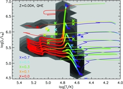
We do not follow rotational mixing in detail but rather adopt a simple parameterisation in which we assume a star is either not mixed or fully mixed depending on binary mass transfer (see next section). If the mass transfer from a companion exceeds 5% of a star’s initial mass, it is assumed to lead to either rejuvenation and/or quasi-chemically homogeneous evolution (QHE). Rejuvenation is the consequence of rapid mixing of new material into the stellar core, resetting its evolution to the zero-age main sequence, thereafter the star evolves normally. QHE follows if the rotational mixing continues after mass transfer ends, disrupting the formation of shell burning and other internal processes. We have calculated simple QHE models by assuming certain stars are fully mixed throughout their main-sequence lifetimes. They therefore evolve to higher temperatures during this time, going ‘the wrong way’ on the Hertzsprung–Russell diagram. We assume this evolution is only possible at Z ⩽ 0.004 and for masses above 20 M⊙ (Yoon, Langer, & Norman Reference Yoon, Langer and Norman2006).
The final detail of our single star models is the mass-loss scheme incorporated for stellar winds. There are two aspects of this scheme: first, the mass-loss rate to apply to a star during a certain phase of its evolution, and second, how the mass-loss rates scale with metallicity. In all our models, we apply the mass-loss rates of de Jager, Nieuwenhuijzen, & van der Hucht (Reference de Jager, Nieuwenhuijzen and van der Hucht1988), unless the star is an OB star where we use the mass loss rates of Vink, de Koter, & Lamers (Reference Vink, de Koter and Lamers2001). These are theoretical rates that do not include clumping but do match observed mass-loss rates (e.g. Shenar et al. Reference Shenar2015) and similar calculations including clumping do show that for the luminous O star the rates are unchanged (Muijres et al. Reference Muijres, Vink, de Koter, Müller and Langer2012). For Wolf–Rayet stars, when the surface hydrogen abundance is less than 40% and the surface temperature is above 104 K, we use the mass-loss rates of Nugis & Lamers (Reference Nugis and Lamers2000). At different metallicities, we scale these mass-loss rates by $\dot{M}(Z)=\dot{M}(\text{Z}_{\odot })(Z/\text{Z}_{\odot })^{\alpha }$
and typically use α = 0.5, except in the case of OB stars where α = 0.69 (Vink et al. Reference Vink, de Koter and Lamers2001). There is some evidence that the value should also be greater for Wolf–Rayet stars (Hainich et al. Reference Hainich, Pasemann, Todt, Shenar, Sander and Hamann2015) but this is currently not considered.
$\dot{M}(Z)=\dot{M}(\text{Z}_{\odot })(Z/\text{Z}_{\odot })^{\alpha }$
and typically use α = 0.5, except in the case of OB stars where α = 0.69 (Vink et al. Reference Vink, de Koter and Lamers2001). There is some evidence that the value should also be greater for Wolf–Rayet stars (Hainich et al. Reference Hainich, Pasemann, Todt, Shenar, Sander and Hamann2015) but this is currently not considered.
All our models evolve from the zero-age main sequence up to the end of core carbon burning, or neon ignition for our most massive star models. Less massive models either form carbon–oxygen or oxygen–neon cores and evolve up the Asymptotic Giant Branch (AGB). We do not model AGB thermal pulses in detail nor incorporate specific AGB mass-loss rates at the current time. To do so is difficult with the stars code and requires care to overcome numerical difficulties (Stancliffe, Tout, & Pols Reference Stancliffe, Tout and Pols2004). At the current time, we limit the spatial and temporal evolution of our AGB models and so we do not observe thermal pulses. We find that the cores then grow up to the Chandrasekhar mass and fail when carbon is ignited in the CO core. This is unphysical and leads to overly luminous AGB stars in our populations. In future, we will recalculate these models with realistic AGB mass-loss rates to terminate the evolution earlier or add a routine with in the population synthesis to use rapid synthetic model of AGB evolution (e.g. Izzard et al. Reference Izzard, Tout, Karakas and Pols2004). The latter option would allow us to investigate the importance of AGB stars in more detail.
Our lowest mass models (below approximately 0.8 M⊙) never ignite helium and end their evolution as helium white dwarfs. Models above this mass and up to approximately 2 M⊙ fail at the onset of core-helium burning due to the core being degenerate at this time. Due to the rapid increase of luminosity in degenerate material with the stars code, we are unable to evolve through this event and the models fail. Therefore, to model the further evolution of these stars, we follow the method of Stancliffe, Izzard, & Tout (Reference Stancliffe, Izzard and Tout2005) and create more massive models where helium ignites in only a slightly degenerate core, we then decrease the mass of the star and allow the helium core to grow out until our model matches the parameters of the last failed helium-flash model. We combine these tracks to make the evolution track complete the possible evolutionary paths of these intermediate mass stars. This is a reasonable approximation as recent more detailed calculations indicate that the helium flash does not explode the star nor cause significant structural changes (Mocák et al. Reference Mocák, Müller, Weiss and Kifonidis2008).
2.1.2. bpass binary star models
Our binary models are identical to our single star models in nearly every respect but we additionally allow for extra mass loss or gain via binary interactions. We assume the orbits of the binary are circular and thus described by Kepler’s third law such that (M 1 + M 2)/M⊙ ∝ (a/215R⊙)3/(P/yr)2, where a is the orbital separation and P is the orbital period. We assume mass lost in stellar winds removes orbital angular momentum in a spherically symmetric shell around the star losing the mass. Thus, the orbits widen over the evolution of the star. We only follow one star with detailed calculations during the evolution. This avoids wasting computational effort on calculating the evolution of a 1 M⊙ secondary star at the same time as a more rapidly evolving 10 M⊙ primary. During the evolution of the primary star models, we use the single star rapid evolution equations of Hurley et al. (Reference Hurley, Tout and Pols2002) to approximate the secondary’s evolution. When the end state of the primary’s evolution has been established, we then substitute the secondary’s evolution with a detailed model, either using a single star model or calculating a new detailed binary model with a compact remnant, depending on whether the binary is bound or unbound.
The grid of masses we use for primary evolution also ranges from 0.1 to 300 M⊙. We model every decimal mass from 0.1 to 2.1 M⊙, then 2.3, 2.5, 2.7, 3, 3.2, 3.5, 3.7 M⊙, every half M⊙ from 4 to 10 M⊙, then every integer mass to 25 M⊙, then every 5 to 40 M⊙ then 50, 60, 70, 80, 100, 120, 150, 200, and 300 M⊙. The grid of mass ratios, q = M 2/M 1, ranges uniformly from 0.1 to 0.9 in steps of 0.1. We establish initial binary periods with log (P/d) from 0 to 4 in steps of 0.2.
For the secondary models which have a compact companion, the grid of models we calculate is determined from the results of the population synthesis after the first supernova. The grid uses the same array of possible periods as for the primaries, however, the secondary masses are reduced to M 2 = 0.1, 0.2, 0.3, 0.4, 0.5, 0.6, 0.8 M⊙, every integer mass from 1 to 25 M⊙, 25, 30, 35, 40, 50, 60, 70, 80, 100, 120, 150, 200, 300, 400, 500 M⊙. The compact remnant masses are arranged in a grid of log (M rem, 1/M⊙) from −1 to 2 in steps of 0.1.
Our numerical method to account for binary evolution is inspired by the method of Hurley et al. (Reference Hurley, Tout and Pols2002) and was first described in detail in Eldridge et al. (Reference Eldridge, Izzard and Tout2008). However, we have had to modify some of the aspects as they are difficult to implement into a detailed stellar evolution code. The key point in our models when binary evolution becomes very different to that of our single star models is when the radius of the primary star increases and so it fills its Roche Lobe. This is the equipotential surface beyond which any material is no longer most strongly gravitationally attracted to the primary star, and Roche lobe overflow (RLOF) can occur. We allow for this in our models by using the effective Roche lobe radius defined by Eggleton (Reference Eggleton1983), where a star will have an equivalent volume to that of its Roche lobe. At radii beyond this, it will begin to overflow mass towards its companion star. The Roche lobe radius is given by
 $$\begin{equation}
\frac{R_{\rm L1}}{a} = \frac{0.49 q_1^{2/3}}{0.6 q_1^{2/3} + \ln (1+ q_1^{1/3})},
\end{equation}$$
$$\begin{equation}
\frac{R_{\rm L1}}{a} = \frac{0.49 q_1^{2/3}}{0.6 q_1^{2/3} + \ln (1+ q_1^{1/3})},
\end{equation}$$
where q 1 = M 1/M 2. When the star fills its Roche lobe, we determine a mass-loss rate due to overflow of
 $$\begin{equation}
\dot{M}_{R1}=F(M_1) \left[\ln \left(\frac{R_1}{R_{L1}}\right) \right]^3,
\end{equation}$$
$$\begin{equation}
\dot{M}_{R1}=F(M_1) \left[\ln \left(\frac{R_1}{R_{L1}}\right) \right]^3,
\end{equation}$$
where
 $$\begin{equation}
F(M_1)=3\times 10^{-6} [\min (M_1, 5.0)]^2.
\end{equation}$$
$$\begin{equation}
F(M_1)=3\times 10^{-6} [\min (M_1, 5.0)]^2.
\end{equation}$$
The value here was chosen by Hurley et al. (Reference Hurley, Tout and Pols2002) to ensure mass transfer is stable within their code. We also found this to be the case in applying their rate. There has been significant amount of work on the exact details of RLOF (e.g. Ritter Reference Ritter1988; Kolb & Ritter Reference Kolb and Ritter1990; Sepinsky, Willems, & Kalogera Reference Sepinsky, Willems and Kalogera2007) and our model is rather simple. However, upon the onset of RLOF, the stellar model will continue to expand until either CEE occurs or the mass transfer becomes stable. In future, we plan to calibrate the RLOF against observed systems undergoing mass transfer.
This mass is assumed to be transferred to the secondary star or lost from the system. We limit the accretion rate onto the secondary star by assuming it can only accept mass at a rate determined by its thermal timescale, such that $\dot{M_2} \le M_2/\tau _{\rm KH}$
. The rest of the material is assumed to be lost from the system, taking with it angular momentum from its orbit. In the case where the companion is a compact remnant with an initial mass less than 3 M⊙, the accretion rate is limited instead by the Eddington luminosity. Above this mass, we assume that super-Eddington accretion can occur due to the compact remnant being a black hole, where super-Eddington luminosities have been observed. In the Eddington-limited case, any excess material and its angular momentum is lost from the system. These limits are also approximate and a more detailed accretion model will be required in future.
$\dot{M_2} \le M_2/\tau _{\rm KH}$
. The rest of the material is assumed to be lost from the system, taking with it angular momentum from its orbit. In the case where the companion is a compact remnant with an initial mass less than 3 M⊙, the accretion rate is limited instead by the Eddington luminosity. Above this mass, we assume that super-Eddington accretion can occur due to the compact remnant being a black hole, where super-Eddington luminosities have been observed. In the Eddington-limited case, any excess material and its angular momentum is lost from the system. These limits are also approximate and a more detailed accretion model will be required in future.
We do follow the rotation rate of the stars in our code but this has no direct physical consequence in the code beyond QHE due to spin-up in mass transfer in binaries (see Section 2.2.2). We follow the rotation rate to keep track of the angular momentum held by the stars, since as stars approach CEE, the Darwin mechanism can cause CEE to occur (Darwin Reference Darwin1880). While we attempted to implement tidal models such as those in Hurley et al. (Reference Hurley, Tout and Pols2002) based on Hut (Reference Hut1981), we found that the most stable method was to only assume tidal synchronisation once a star fills its Roche lobe. Assuming that the stars synchronise their rotation with the orbit, transferring angular momentum from the stars to the orbit or vice-versa. In future, we will add in a more general model of tidal forces and also allow the rotation to induce extra mixing in the stellar interior.
If RLOF does not stop the increase of the donor star’s radius, or if too much angular momentum is required to spin-up the donor star, then CEE occurs. In our code, CEE is taken to occur in our models when the radius of the primary star is the same as the binary separation. At this point, we switch the orbital evolution to a formalism based on the typical population synthesis model where the result of CEE is determined from comparing the binding energy of the envelope with the orbital energy (Ivanova et al. Reference Ivanova2013). We continue to determine the mass-loss rate from Equation (2) but set an upper mass-loss rate limit of 0.1 M⊙ yr−1 to avoid numerical problems of having such a high mass-loss rate. This unfortunately means we overestimate the CEE timescale in our models. To compare to the typical CEE mechanism, it is assumed that the change in the orbital energy of the binary is equal to the binding energy of the envelope of the star that is lost in the interaction:
 $$\begin{equation}
E_{\rm bind}=\Delta E_{\rm orb}.
\end{equation}$$
$$\begin{equation}
E_{\rm bind}=\Delta E_{\rm orb}.
\end{equation}$$
This can be expressed as
 $$\begin{equation}
\frac{Gm_1 m_{\rm 1, envelope}}{\lambda R_1} = \alpha _{\rm CE} \left(-\frac{G m_1 m_2}{2a_i} +\frac{G m_{\rm 1, core} m_{2}}{2 a_{f}} \right),
\end{equation}$$
$$\begin{equation}
\frac{Gm_1 m_{\rm 1, envelope}}{\lambda R_1} = \alpha _{\rm CE} \left(-\frac{G m_1 m_2}{2a_i} +\frac{G m_{\rm 1, core} m_{2}}{2 a_{f}} \right),
\end{equation}$$
where m 1 and R 1 are the mass and radius of the primary, a i and a f are the initial and final orbital separation, αCE is a const representing the efficiency of the conversion from binding energy to orbital energy and λ is a constant representing how the structure of the star affects its binding energy (de Kool Reference de Kool1990; Dewi & Tauris Reference Dewi and Tauris2000).
In a detailed stellar model, it is difficult to remove the entire envelope in a single timestep. Therefore, we instead allow the mass-loss rate to increase as high as possible and relate the binding energy of the material lost to the change in the orbital energy. We do this by equating the binding energy of the lost material to the change in the orbital energy such that
 $$\begin{equation}
\frac{G(M_1+M_2) \delta M}{R_1} = \frac{G M_1 M_2}{a^2} \delta a,
\end{equation}$$
$$\begin{equation}
\frac{G(M_1+M_2) \delta M}{R_1} = \frac{G M_1 M_2}{a^2} \delta a,
\end{equation}$$
which can be rearranged to give
 $$\begin{equation}
\delta a = \frac{a^2}{R_1}\frac{M_1+M_2}{M_2}\frac{\delta M_1}{M_1},
\end{equation}$$
$$\begin{equation}
\delta a = \frac{a^2}{R_1}\frac{M_1+M_2}{M_2}\frac{\delta M_1}{M_1},
\end{equation}$$
where δa is the change in orbital separation and δM 1 is the mass loss of the surface. The advantage of this method is that the structure of the star is naturally taken account of as we integrate over the removal of the envelope. The disadvantage is that because our time for CEE is a few orders of magnitude too large, other sources of energy may limit how efficient CEE is. However, the efficiency of CEE is uncertain.
Our CEE mechanism is meant to reproduce the envelope ejection and the in-spiral simultaneously. Eventually, we find that CEE either results in removal of the stellar envelope or a merger. If the primary star eventually shrinks within the Roche lobe, the CEE is taken to have ended. Mergers are assumed to occur when the companion star begins to fill its own Roche lobe. At this point, the total mass of the secondary is added to the primary star. We typically find the stars that experience CEE on, or just after, the main sequence tend to merge, while post-main-sequence stars tend to only remove the hydrogen envelope. Also, even in systems that do merge, mass loss prior to the event of the merger means that the final stellar mass is less than the total pre-CEE mass of the binary.
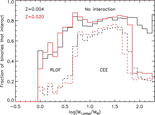
In Figure 1, we show for our fiducial population (as described in Table 1) the fraction of stars that interact, splitting this into those that experience RLOF or RLOF and CEE. We see that at masses of about 5 < M < 40 M⊙, 80% of binaries interact with around 90% of those interactions leading to CEE. We note that for smaller mass ratios, 100% of interactions lead to CEE, while for our largest mass ratios, only 80% lead to CEE. Outside this, mass range RLOF dominates the binary interactions. At high masses, the stellar wind mass loss is already significant and so once RLOF starts, only a little extra mass loss is required to avoid CEE, especially at higher metallicity where stellar winds reduce the number of systems that interact to 30%. Below 5 M⊙ down to approximately 1M⊙, the fraction of interacting systems decreases. This is due to the maximum radius of the stars decreasing so fewer stars fill their Roche lobe and interact. At the lowest masses, below 0.7 M⊙, the interaction fraction decreases to zero due to the stars being smaller than the orbital separation for their evolution within the age of the Universe. This is likely due to our minimum period for our binary models of 1 d, as well simple binary model that does not include processes that would allow for periods to shorten and drive interactions. As a result, with the exception of those in the closest binaries, such sources do not overfill their Roche lobes and so never interact. Stars below ~1 M⊙ never interact in our default model set as they remain compact during their main sequence lifetime, which is long compared to the age of the Universe.
The fraction of primary stars in our fiducial population that experience a binary interaction at two metallicities within the age of the Universe versus the initial mass of the primary star. The solid line represents the total fraction that experience Roche lobe overflow (RLOF). While the dashed line represents the number when RLOF progresses to common envelope evolution (CEE).
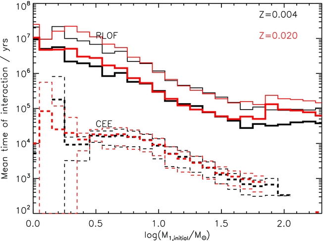
We show the mean duration over which RLOF and CEE episodes occur in our binary models in Figure 2. More massive stars interact on shorter timescales than low mass stars, with RLOF ranging from 105 up to 107 yrs, while CEE has much shorter timescales of 100 to 104 yrs. These times for our CEE events are much longer compared to the very short timescale of days or years that are predicted by dynamical simulations (see Ivanova et al. Reference Ivanova2013) as well as those found from observed events. However, they are significantly shorter than the thermal and nuclear timescales of the stars so they should have little impact on the eventual predictions of binary evolution.
The mean times that binary interactions last for in our fiducial simulation versus the initial mass of the primary star. The solid lines are for RLOF and the dashed lines for CEE. The thick lines are for the mean, the thin lines are at ±1σ. As discussed below, the CEE time are significantly overestimated due to our method of including CEE in our detailed evolution models.
2.1.3. Supernovae and remnants
At the end of the evolution of our models, we check to see what remnant may be produced. Currently, we assume that either a white dwarf, neutron star, black hole, or no remnant will be formed. We assume that a core-collapse supernova will occur if central carbon burning has taken place and the CO core mass is greater than 1.38 M⊙ and the total stellar mass is greater than 1.5 M⊙. If this condition is not met, then the remnant left will be a white dwarf with the mass of the helium core at the end of the stellar model, the secondary star will continue to evolve with a white dwarf in orbit around it.
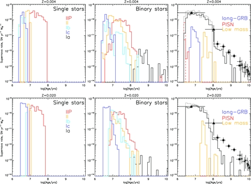
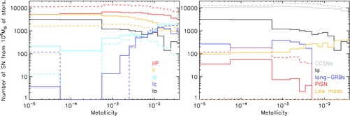
In the case that a supernova occurs the remnant mass is determined by calculating how much material can be ejected from the star given an energy input of 1051 ergs, a typical supernova energy. This method was first outlined in Eldridge & Tout (Reference Eldridge and Tout2004b) which provides more details. The mass that is not unbound goes into the remnant, thus providing a way to estimate the mass of any resultant black hole. This method is similar to others (e.g. Heger et al. Reference Heger, Fryer, Woosley, Langer and Hartmann2003; Ugliano et al. Reference Ugliano, Janka, Marek and Arcones2012; Sukhbold et al. Reference Sukhbold, Ertl, Woosley, Brown and Janka2015; Spera, Mapelli, & Bressan Reference Spera, Mapelli and Bressan2015). For simplicity, neutron star remnants are assumed to have a constant mass of 1.4 M⊙, while remnants more massive than 3 M⊙ are considered to form black holes. Finally, if the helium core mass at the end of evolution is between 64 and 133 M⊙, a pair-instability supernova (PISN) is assumed to occur which completely disrupts the star and leaves no remnant (Heger & Woosley Reference Heger and Woosley2002).
For any system with a core-collapse supernova, we estimate the supernova category as type IIP, II-other, Ib, and Ic. We identify the supernova types as described in Eldridge et al. (Reference Eldridge, Langer and Tout2011) and Eldridge et al. (Reference Eldridge, Fraser, Smartt, Maund and Crockett2013). If the mass of hydrogen in the star is greater than 10−3 M⊙, then we have a type II supernova. If the total mass of hydrogen is greater than 1.5 M⊙ and the ratio of hydrogen mass to helium mass in the progenitor is greater than 1.05, we have a type IIP. When the hydrogen mass is less than 10−3 M⊙, a type Ib/c supernova occurs. If more than 10% of the ejecta mass is helium, then the supernova is assumed to be a type Ib, otherwise it is Ic. This leads to roughly twice as many Ib as Ic supernovae which is in agreement with the most recent attempt to accurately determine this ratio (Shivvers et al. Reference Shivvers2017).
We also determine whether an event is likely to generate a Gamma-ray Burst (GRB) or PISN. For a long-GRB, the star must have experienced QHE and have a remnant mass greater than 3 M⊙. Note that this is only one possible pathway for GRBs and limits their presence in our rate estimates to lower metallicities. Some type Ic supernovae arising from non-QHE systems also likely generate GRBs but we do not account for these. For PISN, we apply mass limits from Heger & Woosley (Reference Heger and Woosley2002) as detailed above. Finally, any progenitor with a final mass between 1.5 and 2 M⊙ is identified as a low-mass progenitor with an uncertain outcome. These events may be faint and rapidly evolving, as described by Moriya & Eldridge (Reference Moriya and Eldridge2016).
We also estimate the type Ia thermonuclear supernova rate by two channels, first selecting out white dwarfs that begin with a mass below the Chandrasekhar limit but then reach or exceed this mass due to binary mass transfer. Second, we count double white-dwarf binaries that merge due to gravitational radiation with the merger time calculated assuming circular orbits and the analytic expressions of Peters (Reference Peters1964). Our resultant rates are highly approximate and we do not consider them rigorous or precise but include them for completeness. We caution that these should be used with care, and in future we may refine our type Ia models further for comparison with other predictions and observational data.
2.2. The population synthesis
2.2.1. Binary distribution parameters
In the population synthesis, the individual stellar models are combined together to make a synthetic stellar population which can be observed and compared to observations of the real Universe. Together with the models described above, we need to know the distribution of initial parameters required to create the population. The three main parameters are the initial mass function (IMF), the initial period distribution, and the initial mass-ratio distribution. Each population is generated at a single initial metallicity. For our fiducial models, we base our IMF on Kroupa, Tout, & Gilmore (Reference Kroupa, Tout and Gilmore1993) with a power-law slope from 0.1 to 0.5 M⊙ of −1.30 which increases to −2.35 above this. The power law slope extends to a maximum initial stellar mass of 300 M⊙, although we note that due to mergers stars, more massive than this can form in our binary populations. Our most massive stars have masses up to 570 M⊙, although these are very rare systems. In addition to this standard model, we also calculate models with two different upper IMF slopes of −2.00 and −2.70, as well as varying the upper maximum initial stellar mass to 100 M⊙. Finally, we calculate a model set with a constant IMF slope of −2.35 from 0.1 to 100 M⊙ [the standard (Salpeter Reference Salpeter1955) IMF], for comparison with previous work.
For the binary populations, we assume a flat distribution in initial mass ratio and log period in all our models. The result of this is that while all of our stars are technically part of a binary population, in many cases the stars evolve as isolated individuals and are never close enough to interact. The actual interacting binary fraction will depend on the physical size of stars at different ages relative to their Roche lobes, and thus on mass and metallicity. Our upper period limit of 10 000 days has been chosen so that about 80% of massive stars (M ≳ 5 M⊙) interact, as shown in Figure 1. From 5 to 0.7 M⊙, this fraction decreases to about 50%. At lower masses, the separation of the orbits with a 1 d minimum is too wide for stars to interact within the age of the Universe. At Solar metallicity, many of the most massive (M ~ 100 M⊙) stars also avoid interactions due to strong mass loss in stellar winds.
Observational constraints on these numbers are uncertain but our estimates of massive star interaction are comparable to the 70% estimated for O stars by Sana et al. (Reference Sana2012). On the other hand, the flat distributions are probably over-simplistic. As discussed by De Marco & Izzard (Reference De Marco and Izzard2017), binary parameters (including the binary fraction) vary with initial mass. While nearly every massive star is in a binary, the binary fraction drops to 20% at lower initial masses below a Solar mass, but the precise binary fraction as a function of stellar mass remains poorly constrained in the literature. In the Milky Way, Sana et al. (Reference Sana2012) found that the observed period distribution is slightly steeper than flat, with a bias towards more close binary systems for O stars. However, Kiminki & Kobulnicky (Reference Kiminki and Kobulnicky2012) found a flatter period distribution in the Cygnus OB2 association that is consistent with Öpik (Reference Öpik1924)’s law, although their results did also suggest a slight preference for short period systems as well. The most recent study by Moe & Di Stefano (Reference Moe and Di Stefano2017) has quantified the period and mass ratio distribution in an extensive compilation of previous works, and finds a slightly different period and mass ratio distribution to that we use. We intend to modify our input distributions accordingly in a future version of BPASS.
The uncertainty in assumed period distribution is degenerate with uncertainties in the assumed model to handle RLOF, common envelope evolution, tides, and other binary specific processes. Hence, we adopt this simple approach based on the well-studied massive star population (Sana et al. Reference Sana2012). If required, it is possible to simulate the effect of more complex populations and binary distributions by varying the mix between our single star and binary populations with age (since stars of different initial masses dominate in different time bins).
We note that, because we assume orbits are circular, our closest observational comparison will be with the semi-latus rectum distribution not the period distribution. As shown by Hurley et al. (Reference Hurley, Tout and Pols2002), the outcome of the interactions of systems with the same semi-latus rectum is almost independent of eccentricity. This is equivalent to assuming that systems are circularised by tidal forces before interactions occur. We only include tides in our evolution models when a star fills its Roche lobe as this can move the system into CEE if there is not enough angular momentum in the orbit to spin up the primary. We assume tidal forces are strong and the star’s rotation quickly synchronises with the orbit. This is of course an approximation and there are recent studies have begun to explore how mass transfer may be different in eccentric systems (e.g. Sepinsky et al. Reference Sepinsky, Willems and Kalogera2007; Bobrick, Davies, & Church Reference Bobrick, Davies and Church2017; Dosopoulou & Kalogera Reference Dosopoulou and Kalogera2016a, Reference Dosopoulou and Kalogera2016b). However, we note that the bpass stellar models have been successfully tested to see if they can reproduce an observed binary system with a slight eccentricity even after mass transfer (Eldridge Reference Eldridge2009).
2.2.2. Binary evolution treatment
We combine all the primary star models together according to these distributions. We then must consider how to account for the secondary stars. We pick out the stars that explode in supernovae by and estimate the remnant mass as described in Section 2.1.3. For remnants less than 3 M⊙, we assume that the remnant receives a kick taken at random from a Maxwell–Boltzmann distribution with σ = 265 km s−1 (see Hobbs et al. Reference Hobbs, Lorimer, Lyne and Kramer2005). For remnants more massive than 3 M⊙, we assume the star has a kick that is reduced by a factor of the remnant mass divided by 1.4 M⊙, assuming that the kicks track a momentum distribution rather than a velocity distribution. There is some observational evidence that black-hole kicks should be weaker than for neutron stars (Mandel Reference Mandel2016). We note that we have also investigated other models of neutron-star kicks but have not yet included these in the released bpass models (see Bray & Eldridge Reference Bray and Eldridge2016).
If the binary is disrupted, then the companion star is modelled as a single star in its further evolution. Conversely, if it remains bound, then the post-supernova orbit is calculated, circularised and a secondary model of a star orbiting a compact remnant is used to represent its future evolution. Eventually, if a second supernova occurs, the same process is repeated so that the parameters of double-compact remnant binaries can be estimated. Note that the secondary may still undergo supernova, even if the primary does not: this possibility is followed and these later events are also considered.
We also check in our models for rejuvenation of the secondary stars. If a secondary star accretes more than 5% of its initial mass and it is more massive than 2 M⊙, then the star is assumed to be spun-up to critical rotation and is rejuvenated due to strong rotational mixing. That is, it evolves from the time of mass transfer as a more massive, zero-age main-sequence star (this is similar to the method used by Vanbeveren, De Loore, & Van Rensbergen Reference Vanbeveren, De Loore and Van Rensbergen1998). At high metallicities, we assume that the star quickly spins down by losing angular momentum in its wind so that there are no further consequences for its evolution. However, with weaker winds at lower metallicity, Z ⩽ 0.004, we assume that the spin down occurs less rapidly and so the star remains fully mixed throughout the main sequence and burns all its hydrogen to helium. We assume the star must have an effective initial mass after accretion >20 M⊙ for this evolution for occur, based on the work of Yoon et al. (Reference Yoon, Langer and Norman2006). We note that we have discussed the importance of these quasi-homogeneously evolving (QHE) stars in greater detail in Eldridge et al. (Reference Eldridge, Langer and Tout2011), Eldridge & Stanway (Reference Eldridge and Stanway2012), and Stanway et al. (Reference Stanway, Eldridge and Becker2016) showing there is strong observational evidence that they exist. We only consider QHE that arises from mass transfer, however, and do not yet include it in tidal interactions as done by Mandel & de Mink (Reference Mandel and de Mink2016) and Marchant et al. (Reference Marchant, Langer, Podsiadlowski, Tauris and Moriya2016). In such a scenario, stars can be spun up by tidal forces acting between two stars in orbital periods of the order of a day, leading to both stars experiencing QHE, this is not yet implemented in bpass.
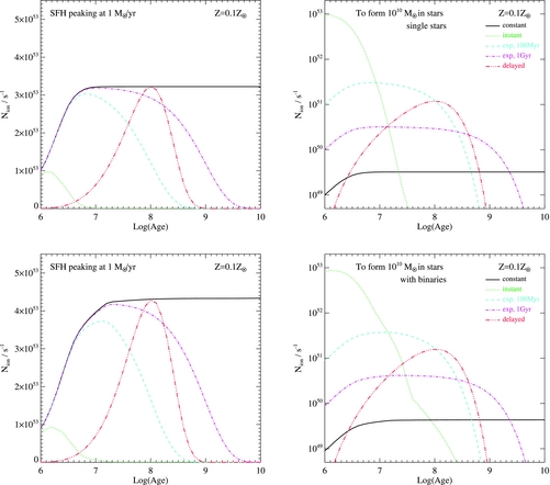
2.2.3. Binary mass function as a function of age
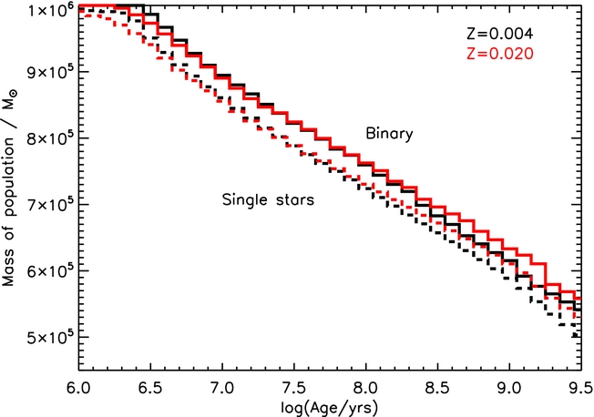
We present some fundamental results from our populations in Figures 3 and 4 which concern the mass in the stars at different different stellar population ages. Figure 3 shows that from an initial 106 M⊙, the total mass of stars in a co-eval binary population slowly decreases with time as stars die and lose mass in stellar winds. We see that the single star populations tend to decrease faster than the binary populations initially, while the binary populations retain more of their mass until the first SN occurs. This leads to an offset between the binary and single star populations which persists until late times. Higher metallicity populations retain more mass at late times. This is because the higher metallicity stars have longer lifetimes due to being less compact with lower central temperatures so burning through their nuclear fuel takes a longer time. Although at early times, the far stronger winds of high metallicity stars means more mass is lost at early times for the higher metallicity population. After this, the stars will evolve along the lower mass pathways at an appropriate rate. The net effect of this is to lead to longer total stellar lifetimes and so a delay in the death of the stars and formation of remnants. By the age of 1 Gyr, a Solar metallicity starburst will have lost 37% (39%) of its initial mass in the binary (single) star evolution case. This is towards the upper end of the ‘return fractions’ of material to the ISM of R ~ 0.4 for a Chabrier (Reference Chabrier2003) IMF and R ~ 0.3 for a Salpeter (Reference Salpeter1955) IMF found by Madau & Dickinson (Reference Madau and Dickinson2014). At 20% of Solar metallicity, both binary and single star return fractions increase by ~2%.
The evolution of the fiducial stellar population mass (the mass contained in stars only) with time. We assume formation of an initial population with total mass 106 M⊙ within the first Myr. Solid lines are for binary populations and dashed lines are for the single-star populations, and results are shown at two metallicities.
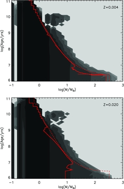
Contour plots showing how the stellar mass function evolves with age. The greyscale contours represent a binary population with each contour being a change in number by an order of magnitude. The lines represent the maximum mass at any given time, the solid line for the initial mass of the star, and the dashed line the final mass of the star with that lifetime.
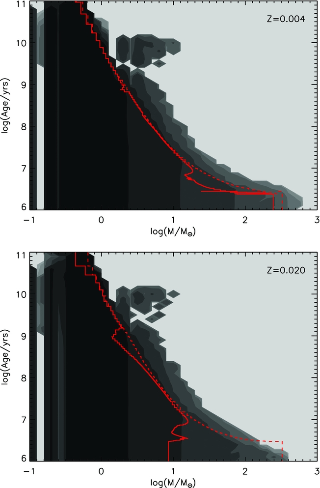
Figure 4 illustrates this effect in greater detail, showing how the stellar mass functions vary with age at the same two metallicities. In both cases, due to rapid mergers of the most massive members of a stellar population, binary populations can have more massive stars than were initially assumed and these can retain mass for longer. At late times, the most massive star is always beyond that expected from single-star populations: the phenomenon that leads to the observation of ‘blue stragglers’ in globular cluster populations. The mass of the most massive star is greater at late times in high metallicity populations, even though at early times the mass of individual stars rapidly decreases due to the stronger mass loss.
We note here that beyond approximately 3 Gyrs, our current models predict a population of more massive stars than would be expected. These are more than twice the maximum mass for a single star population at this age. These are systems where the primary evolved to a white dwarf after rejuvenating its companion star. Our simple method of estimating the rejuvenation age currently uses the age at the end of the model rather than the time of the mass transfer. While this is adequate if the primary explodes in a supernova, it is not for the case where our models include the time on the white-dwarf cooling track.
2.3. Stellar atmospheres and spectral synthesis
While the stellar models described above contain a large amount of detail about the structure, physical conditions (e.g. temperature, surface gravity), and evolution of stars in a population, they provide relatively limited information about their appearance. This is because the physics of stellar atmospheres comprises a second modelling challenge that can be as complex and difficult to calculate as a stellar evolution model. The computational time to calculate a model atmosphere for one set of surface conditions can be the same as the time to calculate the entire evolution of a single stellar model. Therefore, some compromise must be found in connecting the evolution and atmosphere models. Some authors (e.g. Rix et al. Reference Rix, Pettini, Leitherer, Bresolin, Kudritzki and Steidel2004; Groh et al. Reference Groh, Meynet, Ekström and Georgy2014; Topping & Shull Reference Topping and Shull2015) have calculated sets of atmosphere models for specific phases of evolution of their stellar models and interpolate between these. Our solution has been to use pre-calculated grids of atmospheres that we then match to our evolution models to predict their luminous output spectrum. The exception is for extreme cases where no appropriate atmosphere grid is extant: we have created a new set of atmosphere spectra for hot OB stars from existing tools. We detail these grids in Section 2.3.2 below.
2.3.1. Existing model grids
Our base atmosphere models are those of the BaSeL v3.1 library (Westera et al. Reference Westera, Lejeune, Buser, Cuisinier and Bruzual2002). This is a set of atmosphere models that extend over a large range of log g, log T eff, and metallicity. We interpolate between models to predict the spectrum of each star generated by our evolution code. This version only extends over metallicities from [Fe/H] = −2.0 to 0.5. We therefore at our lowest metallcities use the slightly older v2.2 grid of Lejeune, Cuisinier, & Buser (Reference Lejeune, Cuisinier and Buser1998) that extends down to [Fe/H] = −3.5.
We supplement these with Wolf–Rayet (WR) stellar atmosphere models from the Potsdam PoWR groupFootnote 3 (Hamann & Gräfener Reference Hamann and Gräfener2003; Sander et al. Reference Sander, Shenar, Hainich, Gímenez-García, Todt and Hamann2015). We only use WR spectra once the surface hydrogen abundance drops below 40% and the surface temperature is above log (T/K) = 4.45. A key change implemented in bpassv2.0 and v2.1 is that there are now different metallicity nitrogen-dominated (WN) WR atmospheres available (Todt et al. Reference Todt, Sander, Hainich, Hamann, Quade and Shenar2015). In our previous work (such as Eldridge & Stanway Reference Eldridge and Stanway2009), only Solar metallicity were available and we artificially reduced the line luminosities of these models at lower metallicites. We now use the closest metallicity WN models to the stellar models being considered. When Z ⩾ 0.0095, we use the Solar PoWR models, below this limit we use their LMC models and when Z < 0.0035, we use their SMC models. For WC (i.e. carbon-dominated) WR stars, there are still only Solar metallicity models available, but we have not altered these spectra in any way in our current models, using the Solar models at all metallicities. This may lead to slight overestimates in the strength of carbon WC features in low metallicity spectra but the abundances in the stellar atmospheres during the WR phase are relatively insensitive to the initial metallicity (which has a larger effect on mass-loss rate). This will be modified as further PoWR models become available. We switch to the WC models when there is no surface hydrogen and the helium mass fraction drops below 70%.
As in Eldridge & Stanway (Reference Eldridge and Stanway2009), we add in an excess He ii flux for massive of stars as suggested by Brinchmann, Pettini, & Charlot (Reference Brinchmann, Pettini and Charlot2008), since these are under-represented in atmosphere models. For non-WR stars with a surface temperature above 33 000 K and when log g ⩽ 3.676 log (T/K) − 13.253, we increase the He ii stellar wind lines at 1 640 and 4 686 Å by 520 and 33.8 L⊙, respectively. Due to the rarity of these cases, we find this has a minimal effect on the predicted population line fluxes. Interestingly, Crowther et al. (Reference Crowther, Barnard, Carpano, Clark, Dhillon and Pollock2010) have studied He ii emission from massive stars in the Tarantula Nebula and report a very high equivalent width for a young stellar population. We note that with our current prescription as described above, our v2.1 models produce a comparably high equivalent width at slightly older (but similar ages), see Section 6.1 and Figure 28 below.
2.3.2. New O star models
In previous distributions of bpass models, we supplemented the above with a set of O star models generated using the wm basic code by Smith, Norris, & Crowther (Reference Smith, Norris and Crowther2002). We have now recalculated this grid, and extended it, as summarised in Table 2 Footnote 4 .
wm-basic input parameter ranges for new O star grids.
Assumed parameters for identifying different stellar types in the number counts.
For bpass v2.1 models, we have created new wm-basic (Pauldrach et al. Reference Pauldrach, Lennon, Hoffmann, Sellmaier, Kudritzki, Puls and Howarth1998) models based upon the grid determined by Smith et al. (Reference Smith, Norris and Crowther2002). The key differences are that we have extended the metallicity coverage and also added a new sequence of models with a higher surface gravity to better match the evolution code predictions. We have kept the range of temperatures the same (25–50 kK) but now added a grid of high gravity stars with log g = 4.5 (c.f. 4.0 in the earlier grid). This is because we noticed that on the zero-age main sequence, many of our O stars had gravities higher than 4.0 which has a significant effect on the strength of some stellar lines. At low metallicities, our QHE models also increase their surface gravity as they evolve with the stars shrinking as helium is mixed to the surface and the mean-molecular weight increases. Therefore, these new models are important for predicting the correct spectrum.
We also calculate models at every metallicity we consider in bpass rather than simply interpolating between fixed points as before. The key benefit is that we now have spectra at the lowest metallicities when Z = 10−5 and 10−4, where the influence of these massive stars on the synthetic spectrum is strongest. These are beyond the range for which observational validation data is available for stellar atmospheres and so constitute a theoretical extrapolation from better constrained atmospheres at higher metallicity. However, incorporating these gives greater predicting power for stellar populations at these extreme metallicities.
We have made these models available on the bpass website and they have already been used in other published works (e.g. Byler et al. Reference Byler, Dalcanton, Conroy and Johnson2017). We note that only the inclusion of the higher gravity models leads to any significant differences in model outcomes. We find that the ionising flux predictions at low metallicites decrease by about 0.1 dex, but that the far-ultraviolet luminosity of a population increase by a similar amount (see Figure 35 later). This is because the QHE evolution models have more correct atmospheres. These stars evolve to hotter temperatures as they burn hydrogen to helium. These models also allow us to predict O V 1 039 Å lines at very young ages that are comparable to those found in observations (A. Runnholm, private communication).
2.4. bpass model outputs
2.4.1. Spectral energy distributions
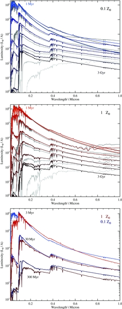
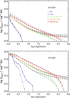
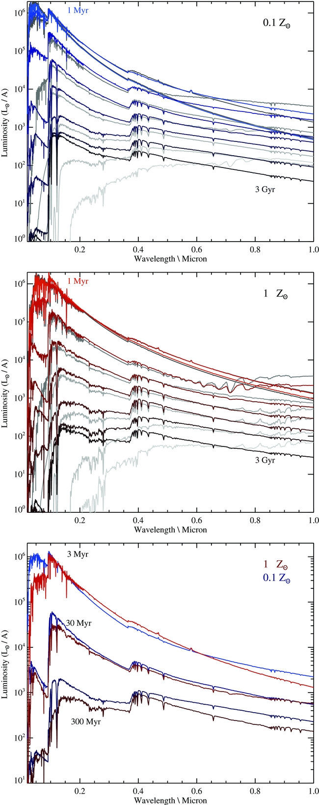
The basic output of bpass is a set of moderately high resolution model spectra, gridded from 1 to 100 000 Å in 1 Å bins and measuring total flux in each wavelength bin in units of L⊙ (i.e. producing a spectrum of F λ in L⊙/Å spanning from the extreme-ultraviolet to far-infrared wavelengths). These are generated for stellar population ages of 1 Myr to 100 GyrFootnote 5 in increments of Δ log (age/yr) = 0.1 where this age is taken relative to the onset of star formation, assuming a co-eval stellar population of total mass 106 M⊙. Examples are shown in Figures 5 and 6, illustrating the optical-infrared spectral energy distributions as a function of age and the extreme ultraviolet as a function of metallicity and binary evolution, respectively.
The synthetic spectra produced for a co-eval population (i.e. instantaneous starburst) at times of 1, 3, 10, 30, 100, 300, 1 000, and 3 000 Myr after star formation. Spectra are shown for binary populations (bold, coloured lines) and single stars (pale, greyscale line), and at metallicities of Z = 0.002 (top) and Z = 0.020 (centre). In the bottom panel, we compare bpass binary models at the two metallicities directly, at ages of 3, 30, and 300 Myr.
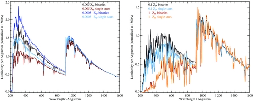
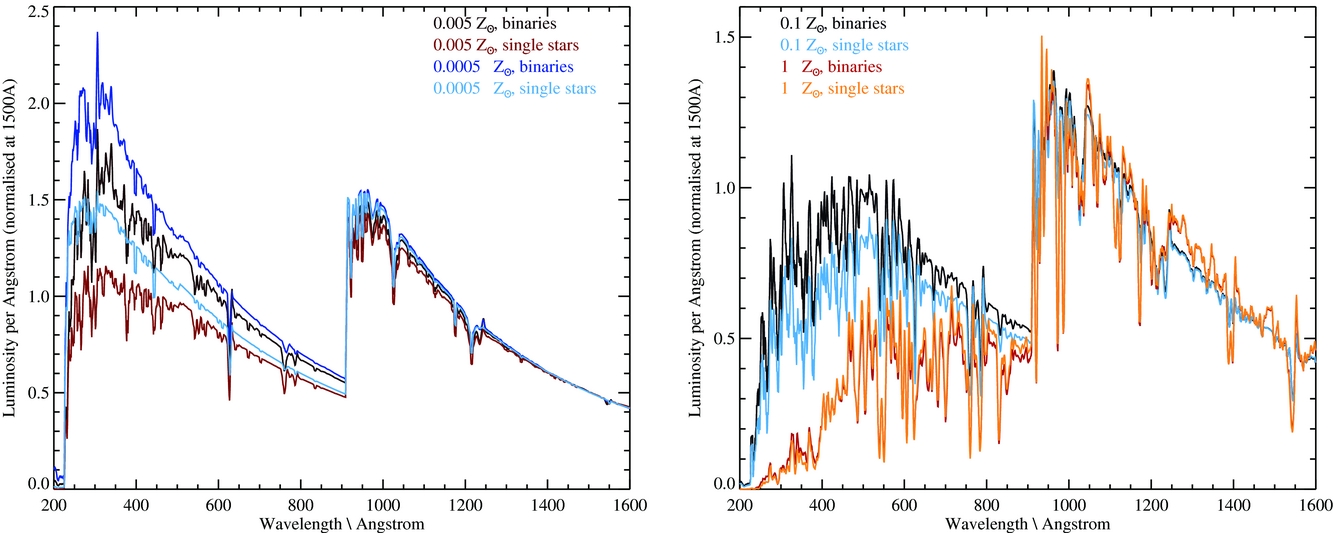
The extreme ultraviolet (200–1 600 Å) spectral region in synthetic spectra produced for a co-eval population (i.e. instantaneous starburst) at a time 30 Myr after star formation. The two panels show the spectra as a function of metallicity (0.05, 0.5% Z⊙ in the left-hand panel, 10 and 100% Z⊙ in the right-hand panel) and bpass single star vs. binary evolution for each metallicity. The effect of binary evolution is to increase the hardness of the spectrum, and hence the ionising photon output (total flux emerging short of 912 Å), particularly at very low metallicities. Synthetic spectra have been scaled to a common luminosity at 1 500 Å.
In Figure 7, we show a direct comparison between the simple stellar population models (i.e. co-eval starbursts) produced by different stellar population synthesis codes at Solar metallicity and allowed to evolve over time. In three panels, bpass single star models are compared to the closest available matching models in metallicity, age, and IMF from publicly available synthesis codes. Perhaps, the most direct comparison is between bpass and the starburst99 models (Leitherer et al. Reference Leitherer1999; Leitherer et al. Reference Leitherer, Ekström, Meynet, Schaerer, Agienko and Levesque2014, hereafter S99), both of which were originally designed and optimised for young starbursts. The S99 models shown here were generated using the non-rotating Geneva 2012/2013 stellar model set and a broken power law IMF with slopes matching our default IMF but with a maximum stellar mass of 100 M⊙.
A comparison between the simple stellar population models (i.e. instantaneous starbursts) produced by different stellar population synthesis codes at Solar metallicity. In three panels, bpass single star models are compared to the closest available match in metallicity, age, and initial mass function from publicly available synthesis codes. These are (top right) the galaxev models of Bruzual & Charlot (Reference Bruzual and Charlot2003), specifically the galaxy templates used to classify galaxies in the Sloan Digital Sky Survey by Tremonti et al. (Reference Tremonti2004), which use a Chabrier IMF; (bottom right) the Maraston (Reference Maraston2005) models, shown here using the Kroupa IMF; (top left) starburst99 models (Leitherer et al), generated with the non-rotating Geneva model set and an IMF matching our power law slopes, and (bottom left) bpass binary star models. Synthetic spectra have been scaled to a common luminosity at 5 000 Å.

We also compare against two SPS codes designed primarily for modelling galaxies. The galaxev models of Bruzual & Charlot (Reference Bruzual and Charlot2003, hereafter BC03) are widely used for modelling mature galaxies and specifically we compare against the galaxy templates used to classify galaxies in the Sloan Digital Sky Survey by Tremonti et al. (Reference Tremonti2004). These use a Chabrier (Reference Chabrier2003) IMF and are built on the Geneva and Padova single star stellar evolution models, combined with a large library of semi-empirical template spectra and additional atmosphere models from the BaSeL atmospheres (Westera et al. Reference Westera, Lejeune, Buser, Cuisinier and Bruzual2002). The Maraston (Reference Maraston2005, hereafter M05) models were designed to confront the thermally pulsating AGB stage in more detail than previous models and use a prescription for fuel consumption to determine the contribution of post-main-sequence stars and their role in determining the near-infrared colours of galaxies. They employ the Cassisi stellar evolution tracks (Cassisi & Salaris Reference Cassisi and Salaris1997; Cassisi et al. Reference Cassisi, Castellani, Ciarcelluti, Piotto and Zoccali2000), BaSeL atmospheres (Lejeune et al. Reference Lejeune, Cuisinier and Buser1998), and a Kroupa (Reference Kroupa2001) broken power law IMF similar to ours (with an upper power law slope of −2.30 where we use −2.35, and a maximum mass of 100 M⊙).
As the figure demonstrates, the bpass single star models are very similar to all three other synthesis models at ages of <1 Gyr and in the ultraviolet, where the models are dominated by massive stars. The BC03 models are slight outliers, appearing redder at very young ages (<10 Myr) than any of the other model sets. Our single star models remain similar to the output of other codes at a matching age through the blue optical bands, with subtle differences in the IMF and evolutionary timescales assumed for the most massive stars by different evolution codes leading to our single star models being slightly bluer than S99 and M05 models but redder than BC03 models at ages of ~10–100 Myr.
bpass models begin to diverge significantly from the other model sets in the red-optical and longwards at stellar population ages of more than a few times 100 Myr. At these ages, the light from our single star populations are dominated by evolved massive stars, primarily AGB stars, whose molecular line features are clearly visible in the composite SED. Perhaps unsurprisingly, our models are most similar in the infrared to the M05 models, which are also heavily influenced by the AGB phase, but we see a stronger effect still. Realistically, this comparison suggests that AGB stars are over-represented in our co-eval single star populations (either in terms of number or luminosity) at ages >1 Gyr. In our favoured binary models (shown in the fourth panel of Figure 7), the number of AGB stars in a population is suppressed by the effect of binary interactions, but these interactions also keep the spectra rather bluer than those seen in other stellar population synthesis models at late times. We note that extreme caution should be applied when using this version of bpass in the red at ages >1 Gyr as a result, we return to this point in Section 7.10.
2.4.2. Released data products
The spectral energy distributions described above for co-eval simple stellar populations form the core of the bpass v2.1 data release. Composite (i.e. non-co-eval) stellar populations are not provided as a part of our standard release but can be constructed by assuming a star formation history (see Section 6.2). The simplest case is a population forming stars continuously at a constant rate. Here, the only potential difficulty lies in dealing with logarithmically spaced time intervals in the models since the total number of stars to be added to the composite spectrum depends on the width of the interval. Stars contributing to the first time bin (at log(age/yrs) = 6.0) include all members of the population up to age 106.05, the second bin stars in the age range 106.05 to 106.15 yrs and so forth.
We calculate magnitudes for individual stellar models and for our synthetic populations in the standard UBVRIJHK filters, as well as ugriz SDSS filters, FUV(1 566Å), NUV(2 267Å) fluxes, and several HST optical filters at each step. Additionally, we calculate the production rate of ionising photons based on the extreme ultraviolet flux since this is strongly affected by both binary evolution and metallicity [see Figure 6 and Stanway et al. (Reference Stanway, Eldridge and Becker2016)].
Given that our population synthesis tracks all stages of stellar evolution, we are also able to produce corresponding rates of supernovae (separated by type) and information on the compact remnant population and stellar class distribution at each time step.
-
1. Stellar model outputs:
-
a. Binary stellar models with photometric colours.
-
b. New OB stars atmosphere models.
-
-
2. Stellar population outputs (all versus age):
-
a. Massive star type number counts.
-
b. Core collapse supernova rates.
-
c. Yields, energy output from winds and supernovae, and ejected yields of X, Y, and Z.
-
d. Stellar population mass remaining.
-
e. HR diagram (isochronal contours).
-
-
3. Spectral synthesis outputs (all versus age):
-
a. Spectral energy distributions.
-
b. Ionising flux predictions.
-
c. Broadband colours.
-
d. Colour–magnitude Diagram (CMD) making code.
-
-
4. Available on request due to unverified status:
-
a. Approximate accretion luminosities from X-ray binaries.
-
b. A limited set of nebula emission models.
-
All outputs of the current bpass v2.1 data release can be found at http://bpass.auckland.ac.nz and are mirrored at http://warwick.ac.uk/bpass. The results can also be found at the PASA datastore.
3 OBSERVATIONAL VALIDATION ON RESOLVED STARS AND STELLAR POPULATIONS
It is vital to test the accuracy and predictive power of our models as far as we can. Because the most basic component of bpass are the stellar models these are the first element we consider. In this section, we explore a number of observational constraints on individual stars and resolved stellar populations, and use these to validate our models, commenting on successes and limitations of the bpass stellar models.
3.1. Main-sequence stars and eclipsing binaries
A powerful validation test is the comparison of our models to double-lined spectroscopic eclipsing binaries. From these systems, it is possible to accurately determine the radius, luminosity, surface temperature, mass, and distance of the stars, making them amongst the best understood individual stars other than the Sun. We use the list compiled by Southworth (Reference Southworth, Rucinski, Torres and Zejda2015)Footnote 6 that builds upon that of Andersen (Reference Andersen1991) which listed systems with observational uncertainties less than 3%.
The scope of the Southworth (Reference Southworth, Rucinski, Torres and Zejda2015) catalogue is explicitly limited to stars which do not show clear evidence for evolution affected by mass transfer. In this paper, we supplement this sample with data on three additional (non-eclipsing) binary systems: VV Cephei (Wright Reference Wright1977; Bauer, Stencel, & Neff Reference Bauer, Stencel and Neff1991; Hack et al. Reference Hack, Engin, Yilmaz, Sedmak, Rusconi and Boehm1992; Bennett et al. Reference Bennett, Brown, Fawcett, Yang, Bauer, Hilditch, Hensberge and Pavlovski2004; Hagen Bauer, Gull, & Bennett Reference Hagen Bauer, Gull and Bennett2008; Bennett Reference Bennett, Leitherer, Bennett, Morris and Van Loon2010), WR20a (Rauw et al. Reference Rauw2005), and γ-Velorum (North et al. Reference North, Tuthill, Tango and Davis2007). We include these as they contain very masive stars, a WR star and a red supergiant (RSG). Since we are concerned with the effects of very massive stars, it is important to include these in our model tests. We have also supplemented the data with recent observations of white dwarfs in eclipsing binaries from Parsons et al. (Reference Parsons2017) to test the validity of modes in this evolutionary state.
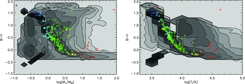
In Figure 8, we present contour plots of the density of stars expected from ongoing constant star formation for 10 Gyr at Solar metallicity for the Hertzsprung–Russell diagram, the spectroscopic HR diagram and the log g–log (T/K) diagram. Contours are defined as timescale and IMF weighted probabilities of a star occurring at a given point in parameter space. Each contour represents an order of magnitude difference in stellar number density. In each of these plots, representative stellar evolution tracks are shown, as well as the observed eclipsing binaries. Pairs of stars in a binary system are plotted linked by a thin line. Both tracks and observational data are colour-coded by stellar mass. In general, the agreement by eye is good. Most stars occur in the regions expected for main-sequence evolution, with a few objects consistent with identification as helium-burning giants. As expected, the white-dwarf sample of Parsons et al. (Reference Parsons2017) populates the white-dwarf cooling track in our models.
Eclipsing binaries overplotted on evolution tracks for our binary models (greyscale, indicating the range of outcomes for a given initial mass). The observed population of eclipsing binaries are overplotted as small symbols, with lines linking binary companions. We show representative tracks for the photometric Herzsprung–Russell diagram and its spectroscopic counterpart, together with the log g-log T plane. The representative tracks have masses of 1, 3, 5, 10, 20, 30, 50, and 80 M⊙ and both they and the observed data are colour coded by mass. The observational data is mainly taken from Southworth (Reference Southworth, Rucinski, Torres and Zejda2015) and supplemented by VV Cephei, WR20a, and γ-Velorum, as well as the white-dwarf sample of Parsons et al. (Reference Parsons2017) as detailed in the text.

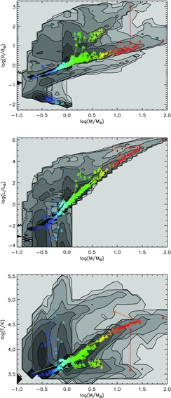
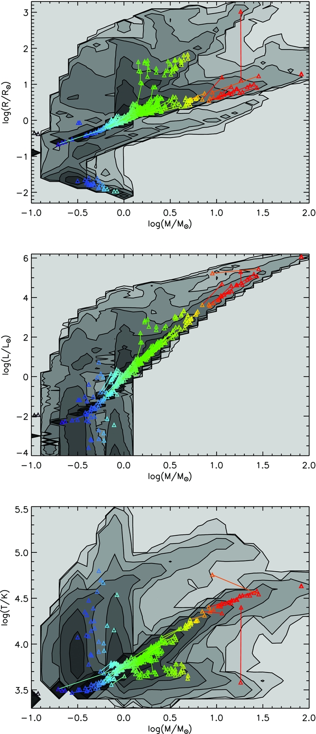
In Figure 9, we take the comparison slightly further and plot each derived parameter (radius, luminosity, and temperature) versus mass. Observational data shows a clear trend that relates mass to each of these parameters: these are derivable from stellar structure theory by homology assumptions. Again qualitative agreement with the bpass stellar models is generally excellent. The poorest agreement between models and data is for the WR binary star γ-Velorum. This is not an eclipsing binary and thus the radius estimate is dependent on calculation from a model atmosphere so over-interpretation of this discrepancy may be unwise. The radii of WR star models is uncertain due to the effect of clumping in the outer envelope. Models with this effect included increase the radii and decrease the temperature of WR stars, improving agreement (McClelland & Eldridge Reference McClelland and Eldridge2016). By contrast, both the highest mass star, WR20a, and the RSG, VV Cephei, show observational properties consistent with the predicted properties of these stars in our models.
Eclipsing binaries overplotted on evolution tracks for our binary models (greyscale, indicating the range of outcomes for a given initial mass). The observed population of eclipsing binaries are overplotted as small symbols, with lines linking binary companions, coloured by metallicity. We show distributions for key parameters. The observational data is mainly taken from Southworth (Reference Southworth, Rucinski, Torres and Zejda2015) and supplemented by VV Cephei, WR20a, and γ-Velorum, as well as the white dwarf sample of Parsons et al. (Reference Parsons2017) as detailed in the text.
Besides eclipsing binary stars, the observational samples with well-constrained physical properties suitable for testing our models become less clearly defined. For most stars, we do not have a precise estimate of distance, this of course will change with time as Gaia continues its mission. Instead we can use the work of Langer & Kudritzki (Reference Langer and Kudritzki2014) who defined the spectroscopic HR diagram, we have already shown an example of this in Figure 8. This diagnostic involves a gravity-weighted luminosity. Combining the Stefan–Boltzmann law, L = 4πR 2σT 4 eff, with the surface gravity, g = GM/R 2, it can be shown that
 $$\begin{equation*}
\log \left(\frac{T^4_{\rm eff}}{g}\right)=\log \left(\frac{T^4_{\rm eff} R^2}{\text{GM}}\right) = \log \left(\frac{L}{4\pi \sigma M}\right).
\end{equation*}$$
$$\begin{equation*}
\log \left(\frac{T^4_{\rm eff}}{g}\right)=\log \left(\frac{T^4_{\rm eff} R^2}{\text{GM}}\right) = \log \left(\frac{L}{4\pi \sigma M}\right).
\end{equation*}$$
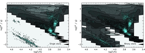
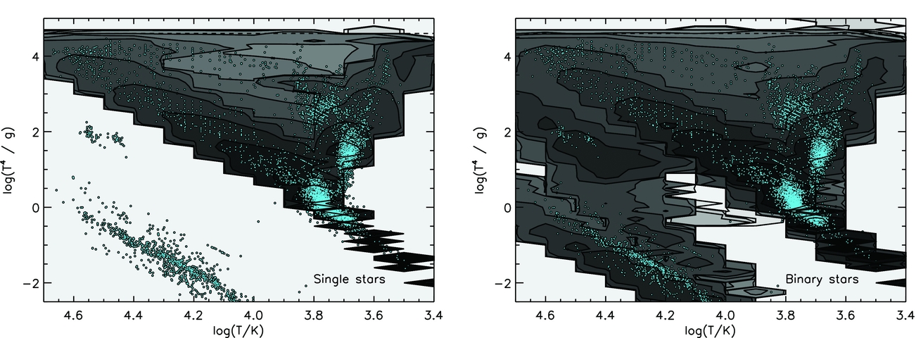
This is a luminosity-related variable that can be derived from the spectrum of a star alone, without needing to determine the precise distance to the object, and thus significantly expands the sample of objects against which models can be tested. Here, we consider the Galactic stellar catalogue of Castro et al. (Reference Castro, Fossati, Langer, Simón-Díaz, Schneider and Izzard2014) for massive stars with half-Solar metallicity and above as well as those that do not have metallicities. In Figure 10, we compare both bpass single and binary star predictions to the distribution of observed stars in this parameter space. In general, the agreement is good. In the binary populations, at Solar metallicity, we see only small differences in the hydrogen burning main sequence and the red giant branch relative to the single star models. The binary models predict more post-main-sequence stars, especially blue and yellow supergiants. We are additionally able to predict the number of helium burning sdB/O stars, as well as the position of the white-dwarf cooling track. The slight offset on the HR diagram between our white dwarf models and some of the observations is likely due to unknown white-dwarf metallicities and perhaps gravitational settling that will affect the surface appearance of these stars and is not included in our models.
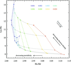
Spectroscopic HR diagrams for single (left) and binary (right) stellar populations. This diagram replaces bolometric luminosity with the gravity-weighted flux as described by Langer & Kudritzki (Reference Langer and Kudritzki2014). Here, we overplot the data from Castro et al. (Reference Castro, Fossati, Langer, Simón-Díaz, Schneider and Izzard2014) for Galactic stars near Solar metallicity as small blue points. Each contour represents an order of magnitude in number density of objects.
3.2. Post main-sequence, giant, and evolved stars
While stars spend most of their time on the main sequence, the evolution after this phase can have significant implications for the observational characteristics of a stellar population, particularly if the population is unresolved. In this subsection, we discuss how well we reproduce observed properties of RSGs, blue supergiants (BSGs), and WR stars.
The figures used in this section are made in a similar way to the figures in the previous section but focus on different sub regions of the HR diagram for comparison with different observational samples. We limit the upper age of the population to 100 Myrs for RSGs and 10 Gyr otherwise.
3.2.1. Red and blue supergiants
In Figure 11, we compare population density contour plots and 1 000-d period stellar tracks to observed RSGs in the SMC, LMC, M31, and M33 taken from Levesque et al. (Reference Levesque, Massey, Olsen, Plez, Josselin, Maeder and Meynet2005), Massey et al. (Reference Massey, Silva, Levesque, Plez, Olsen, Clayton, Meynet and Maeder2009), Neugent et al. (Reference Neugent, Massey, Skiff and Meynet2012), Drout et al. (Reference Drout, Massey and Meynet2012), and Massey & Evans (Reference Massey and Evans2016). The fit is qualitatively good. Based on the comparison between data and model contours, we infer that RSGs typically have masses ⩽25 M⊙. At higher masses, the number of observed supergiants decreases, especially in the SMC and LMC, which are at lower typical metallicities than the Milky Way. At all metallicities, the presence of relatively long period (~1 000 d) binaries appears to prevent RSGs from getting too cool. The details of the RLOF and CEE experienced by these stars is described in Section 2.1.2. Binary interactions tend to only occur for the higher mass tracks at this orbital period, with RSGs below 12 M⊙ largely unaffected by being in such a wide binary. The reason being that while the RSGs have similar temperatures, the more massive and luminous RSGs are larger in radius and thus more likely to experience a binary interaction.
HR diagrams focused on the red supergiant branch at three metallicities for single and binary stars. The observational data is from the samples taken from Levesque et al. (Reference Levesque, Massey, Olsen, Plez, Josselin, Maeder and Meynet2005), Massey et al. (Reference Massey, Silva, Levesque, Plez, Olsen, Clayton, Meynet and Maeder2009), Neugent et al. (Reference Neugent, Massey, Skiff and Meynet2012), Drout, Massey, & Meynet (Reference Drout, Massey and Meynet2012), and Massey & Evans (Reference Massey and Evans2016). For Z = 0.004, we use RSGs from the SMC, for Z = 0.008, we use those in the LMC and M33, for Z = 0.020, we use those from the Galaxy and M31. The tracks and observed WR stars are colour coded to show the surface hydrogen mass fraction. The tracks have masses of 8, 10, 12, 15, 20, 30, 40, and 60 M⊙, the binary star tracks shown have initial periods of 1 000 d and an initial mass ratio of 0.5, the section outlined in white indicates when a binary interaction is taking place. Each greyscale contour represents an order of magnitude in number density of objects.
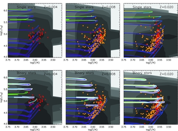
The next stars to consider are BSGs. These are post-main-sequence objects that lie just off the main sequence at high luminosities as the stars travel through the Hertzsprung gap. Meynet et al. (Reference Meynet, Kudritzki and Georgy2015) investigated these stars using rotating models; here, we investigate similar evolutionary tracks but for binary models. We demonstrate in Figure 12 that we reproduce the trend in bolometric luminosity versus flux weighted gravity for these sources. The BSG models contributing to contours are selected from stellar models that are initially more massive than 8 M⊙, have M bol ⩽ −4, 4.4 ⩾ log (T eff/K) ⩾ 3.9, X surf ⩾ 0.4, log g ⩽ 3.5, and have completed core hydrogen burning. The observed BSG sample (Kudritzki et al. Reference Kudritzki, Urbaneja, Bresolin, Przybilla, Gieren and Pietrzyński2008; Urbaneja et al. Reference Urbaneja, Kudritzki, Bresolin, Przybilla, Gieren and Pietrzyński2008; U et al. Reference U, Urbaneja, Kudritzki, Jacobs, Bresolin and Przybilla2009; Kudritzki et al. Reference Kudritzki, Urbaneja, Gazak, Bresolin, Przybilla, Gieren and Pietrzyński2012, Reference Kudritzki, Urbaneja, Gazak, Macri, Hosek, Bresolin and Przybilla2013; Hosek Jr. et al. Reference Hosek2014; Kudritzki et al. Reference Kudritzki, Urbaneja, Bresolin, Hosek and Przybilla2014) is split between the three plots at log (Z/Z⊙) ⩽ −0.55 for Z = 0.004 and log (Z/Z⊙) ⩾ −0.2 for Z = 0.020 and in between these limits for Z = 0.008. In general, the observed BSGs lie over the contours of greatest probability in our models. At the highest bolometric luminosities and at Z = 0.002, the data deviates to slightly higher flux-weighted gravity than our models predict. At Z = 0.020, this trend reverses, with the data suggesting slightly lower flux-weighted gravities. This may result from a small discrepancy in mass, or perhaps metallicity between models and data.
Flux-weighted gravity versus bolometric luminosity for blue supergiants. Observational data taken from the compilation of Meynet, Kudritzki, & Georgy (Reference Meynet, Kudritzki and Georgy2015). Left-hand panel is for Z = 0.004, central panel for Z = 0.008, and right-hand panel for Z = 0.020. The tracks have masses of 3, 5, 8, 10, 12, 15, 20, 30, 40, and 60 M⊙, and an initial binary period of 100 d.
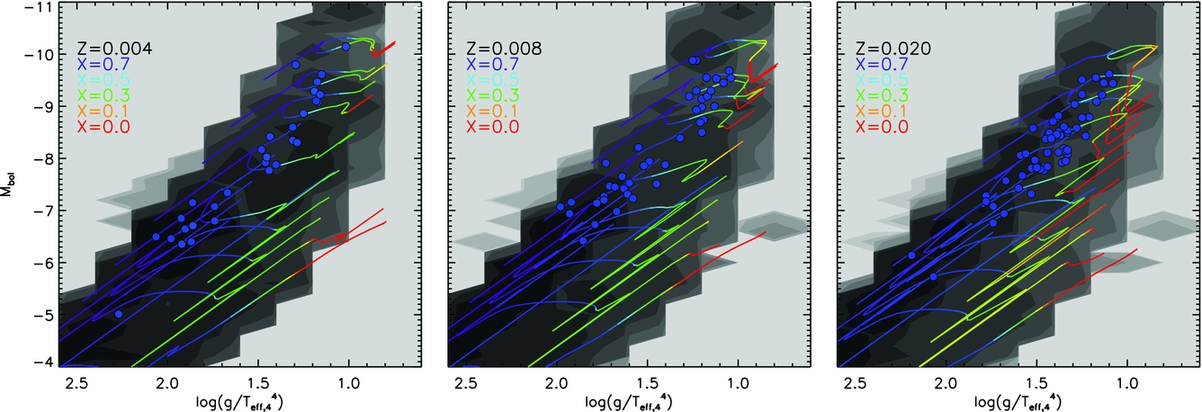
3.2.2. Wolf–Rayet stars
Further comparisons can be made to WR stars, especially those that are hydrogen-free. We show the HR diagrams for these stars in the panels of Figure 13 at three different metallicities and for single stars and binary populations. Here the contours represent where we expect to observe completely hydrogen-free stars which corresponds to when the tracks are red. The binary tracks in the right-hand panels now have an initial period of 100 d with a mass ratio of 0.5. These are compared against observed WR stars (Crowther et al. Reference Crowther, Dessart, Hillier, Abbott and Fullerton2002; Hamann, Gräfener, & Liermann Reference Hamann, Gräfener and Liermann2006; Sander et al. Reference Sander, Hamann and Todt2012; Tramper et al. Reference Tramper2013; Hainich et al. Reference Hainich2014; Hainich et al. Reference Hainich, Pasemann, Todt, Shenar, Sander and Hamann2015; Shenar et al. Reference Shenar2016). Figure 13 illustrates a known outstanding problem in that many WC stars and WN stars have cooler surface temperatures than predicted by stellar evolution models (Hamann & Gräfener Reference Hamann and Gräfener2003; Sander et al. Reference Sander, Hamann and Todt2012). One possible explanation is that clumping in the outer convective zone of the star may inflate the envelope (Gräfener, Owocki, & Vink Reference Gräfener, Owocki and Vink2012; McClelland & Eldridge Reference McClelland and Eldridge2016). When we look at the comparison between our stellar models and observed WR stars, especially for hydrogen-free objects, in Figure 13, we see the luminosity distribution is reproduced, but we see the expected temperature offset at LMC and Galactic metallicities, especially for the hydrogen-free WC stars (shown as triangles). Interestingly, we do not see so large an offset in the SMC where the abundances of the observed sources are similar to those of nearby stellar tracks.
HR diagrams with contours plots showing the expected location of hydrogen-free Wolf–Rayet stars in the SMC (top), LMC (middle), and Galaxy (bottom) panels. The left-hand panels are for the single star populations and the right-hand panels for binary populations. The tracks and observed WR stars are colour coded to show the surface hydrogen mass fraction. The observations are taken from Hamann & Gräfener (Reference Hamann and Gräfener2003), Sander, Hamann, & Todt (Reference Sander, Hamann and Todt2012), Hainich et al. (Reference Hainich, Pasemann, Todt, Shenar, Sander and Hamann2015), and Shenar et al. (Reference Shenar2016). Triangles indicate WC/WO stars, crossed WN stars, diamonds indicate the WN3/O3 stars from Neugent et al. (Reference Neugent, Massey, Hillier and Morrell2017). The tracks have masses of 15, 20, 25, 30, 40, 60, 100, and 300 M⊙, and an initial binary period of 100 d.
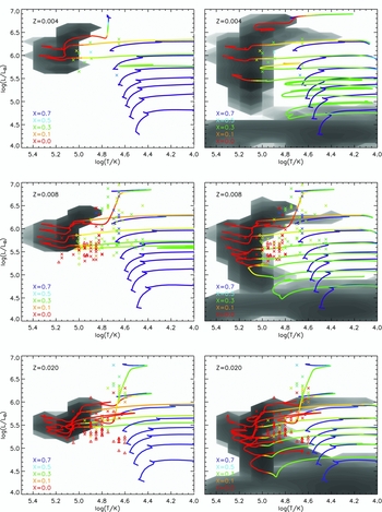
McClelland & Eldridge (Reference McClelland and Eldridge2016) found that inflation can decrease the surface temperature of a WR stars by about 0.2 dex. As can be seen, this is roughly the temperature decrease required to secure better agreement between the models and the observed WR stars. We do not include this effect in our current bpass models as the physics is uncertain and we are still unclear whether the fitting method of the atmosphere models is entirely correct. If inflation effects are metallicity dependent, this may explain why the offset is less pronounced at LMC metallicities. The relatively minor difference in temperature has little effect on the integrated spectrum of a stellar population, but we note that caution is needed when evaluating the properties of an individual WR star through model fitting.
Recently, Neugent et al. (Reference Neugent, Massey, Hillier and Morrell2017) discovered a new class of WR stars, WN3/O3 stars. We have included them in the LMC panels in Figure 13 as diamond symbols. We see that the models agree well with the observed luminosity, temperature, and surface composition of both binary and single star stellar tracks. This suggests therefore that these are typical WR stars, however their reported mass-loss rates indicate that the rates used in our models may be too high for such stars. We note that it has been suggested by Smith, Gotberg, & de Mink (Reference Smith, Gotberg and de Mink2017) that these may be less massive helium stars rather than WR, which would also be consistent with our binary models. However, the projected distance from O stars they find of a few hundred parsecs could be understood if these objects are also runaway stars. The results of Eldridge et al. (Reference Eldridge, Langer and Tout2011) for type Ib/c SN progenitors suggest that 10 to 20% of WR stars could travel 100 parsecs, and further, away from their birth places (see their Figure A3).
3.2.3. Quasi-chemically homogenous evolution
As discussed in Section 2.1, a small subset of evolved stars are expected to undergo quasi-homogenous evolution and these models too require observational verification. QHE stars for the most part should look identical to more normal WR stars so will be difficult to separate out, and indeed there are no clearly unambiguous examples known. However, their chemical composition may aid identification. Most typical WR stars form helium cores and then lose their hydrogen envelopes. By comparison, QHE stars, when hydrogen rich, are still core-hydrogen burning so will exist for a longer period of time and also have different compositions at locations on the HR diagram close to the traditional hydrogen-burning main sequence.
In Figure 14, we compare the QHE tracks (shown with bold lines and evolving towards higher temperatures) to standard binary evolution tracks (thin lines, evolving first towards lower temperatures). Contours give the probability distribution of all models in our population synthesis which experience QHE. We see that in general the WR stars are in better agreement with the standard evolution tracks than with QHE models. As noted by Hainich et al. (Reference Hainich, Pasemann, Todt, Shenar, Sander and Hamann2015) and Shenar et al. (Reference Shenar2016), it appears that mass-loss rates may have been slightly overestimated in current models. We see however that the lowest luminosity WR star in this sample is much cooler and more hydrogen rich than the other stars. Its location matches quite closely that of our 40 M⊙ QHE track. This star, AB2, is perhaps the best candidate for a QHE (by mass transfer) star in the nearby Universe and deserves further study (Martins et al. Reference Martins, Hillier, Bouret, Depagne, Foellmi, Marchenko and Moffat2009; Hainich et al. Reference Hainich, Pasemann, Todt, Shenar, Sander and Hamann2015).
HR diagram showing the evolution of QHE models at Z = 0.004 compared to the properties of WR stars in the SMC. Crosses indicate WR stars, asterisks are the O star companions from Shenar et al. (Reference Shenar2016). Colour coding is the surface hydrogen abundance. The thicker tracks are for QHE stars, while thinner tracks are standard binary models. The tracks have masses of 20, 25, 30, 40, 60, 100, 300 M⊙ and an initial binary period of 100 d.

3.2.4. Stellar-type ratios
An important validation test to consider is not just whether we reproduce the location of these stars in the HR diagram but whether we reproduce the correct relative numbers. We show in Figure 15 the predicted numbers of massive stellar types (log(L/L⊙) > 4.9), specifically O stars, BSG, YSG, RSG, WR (total), WN, and WC stars as a function of metallicity for constant star formation and also with age assuming an instantaneous starburst. We define the surface parameters of each stellar type in Table 3. O stars and BSGs are the most populous classes at all metallicities, as expected for the stars that exist when stars burn hydrogen to helium. The numbers of the remaining subtypes vary smoothly with metallicity. In general, the WR stars decrease in number at lower metallicities since the formation of these requires mass loss and the action of stellar winds is less efficient in the absence of metals. We note that binary populations, which provide another avenue for mass loss, exhibit a weaker metallicity trend than the single star population.
Number of massive stars with log (L/L⊙) > 4.9 of different stellar types from our fiducial populations. The stellar types are defined in Table 3. Dashed lines are for single stars, solid binary populations. The dot-dashed line for the WR population includes lower luminosity, lower mass stars which otherwise satisfy the temperature and surface abundance criteria for WR stars. Top panel shows the metallicity variation of stellar type ratios assuming a population undergoing continuous star formation at a rate of 1 M⊙ yr−1. Lower panels show time evolution of an instantaneous burst (i.e. a single-aged stellar population) at two different metallicities. Where lines are interrupted, zero stars in that type category remain in the (finite-sized) population in a given time bin.
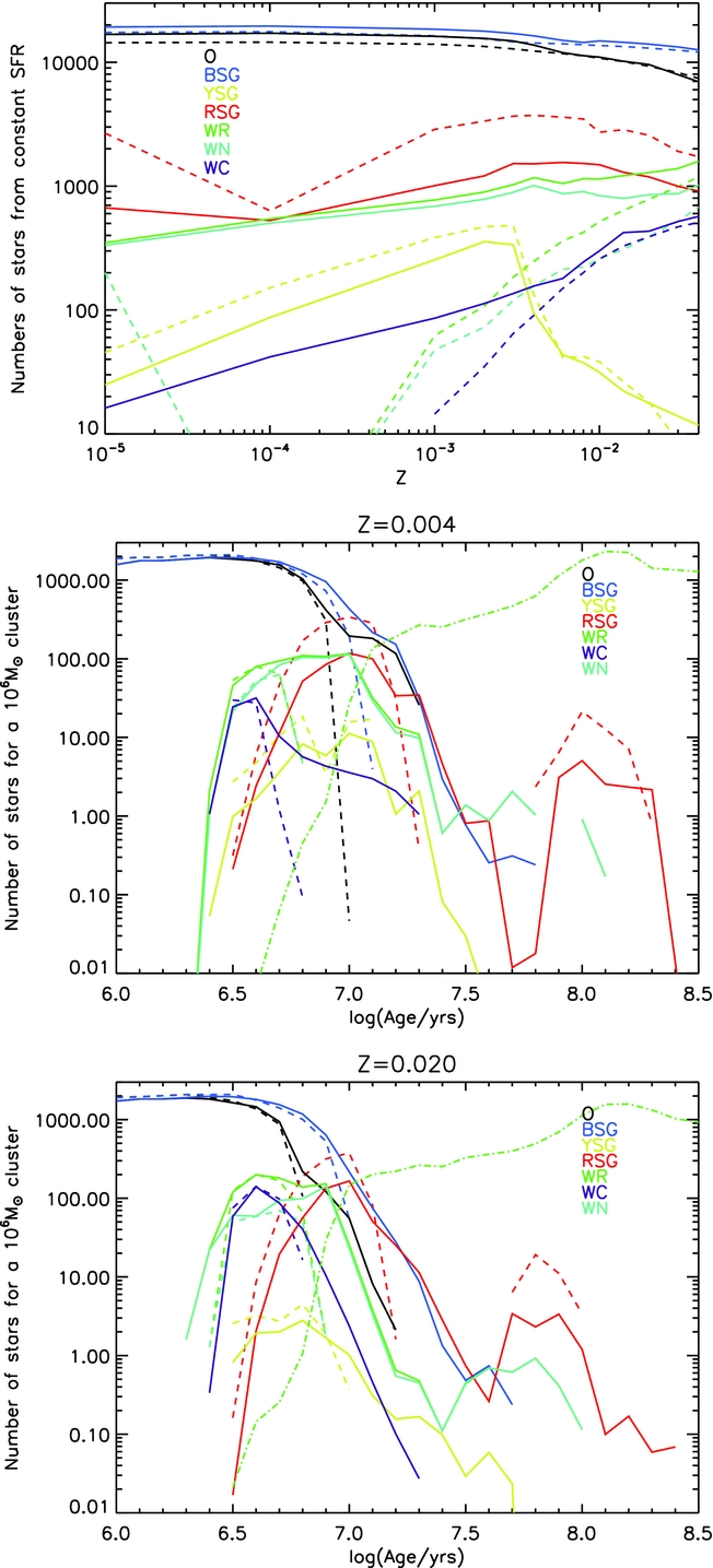
Considering the evolution of an instantaneous burst, we see that the different stellar types appear at different stellar population ages. Binary interactions extend the lifetime of the WR stars, especially WC stars, to later times. This highlights the difficulty of precisely aging a stellar population from the fact that WR stars exist alone. In our RSG numbers, we see a late time peak at around 100 Myrs in both metallicities shown in the figure. This is due to a small contribution of AGB stars at these ages which meet the temperature and luminosity constraints for selection as RSGs in our model. Observationally, they would also be difficult to distinguish.
Similar predictions to these have been used for many years to constrain stellar models by comparing the model to the number of different stellar types observed in an entire galaxy, ideally at known metallicity (e.g. Maeder & Meynet Reference Maeder and Meynet1994). Here, we perform a similar test, comparing bpass predictions of the WR to O, BSG to RSG, WR to RSG, and WC to observed WN ratios in nearby galaxies (see figure caption for data sources). One problem with such comparisons is uncertainty in how complete each observational sample is, especially for the WR to O star ratio where both stellar types are hot and difficult to find in optical surveys. The comparison will also be somewhat dependent on the star formation history and here we assume continuous star formation at a constant rate.
The panels in Figure 16 show the current bpass v2.1 predictions (black and blue lines given two IMF mass limits, M max = 100 or 300 M⊙) for these ratio in comparison to the observed ratios which exist and also previous bpass v1.0 predictions (red line). For all these number and stellar type number ratios, we only include stars with log (L/L⊙) > 4.9, since Massey & Olsen (Reference Massey and Olsen2003) used this as a luminosity cut-off to make sure that AGB stars are not included in their sample (although we note that a small number of our AGB models do indeed satisfy this criterion). WR stars do not typically have luminosities below this value (McClelland & Eldridge Reference McClelland and Eldridge2016). It is consistent to also apply this to our O star number predictions for comparison to the data, but we note that this excludes the many O stars that lie just below this limit in our models. In the upper left panel of Figure 16, we include predictions for the WR/O ratio that include all O stars as well as only those above our luminosity limit (dotted and dot-dashed lines for binary and single stars, respectively).
Stellar-type number ratios for massive star populations. Solid lines show bpass binary models and dashed lines show single models. Points with error bars show observational constraints taken from the literature. All ratios include only stars with log (L/L⊙) > 4.9, except the WR/O star ratio where the dotted (binary) and dash-dotted (single) lines include all O stars. The red lines show results for constant star formation from bpass v1.0, while the blue and black lines show similar results from BPASS v2.1 with two different IMFs (M max = 300 and M max = 100 M⊙, respectively). WR/O ratio data is taken from Maeder & Meynet (Reference Maeder and Meynet1994), the BSG/RSG ratio data is from Massey & Olsen (Reference Massey and Olsen2003) and the WR/RSG data comes from P. Massey (private communication). The WC/WN ratio data plotted in blue and red and is taken from Rosslowe & Crowther (Reference Rosslowe and Crowther2015) with the blue points omitting the dusty WC stars. The WC/WN ratios plotted in black are from Meynet & Maeder (Reference Meynet and Maeder2005).
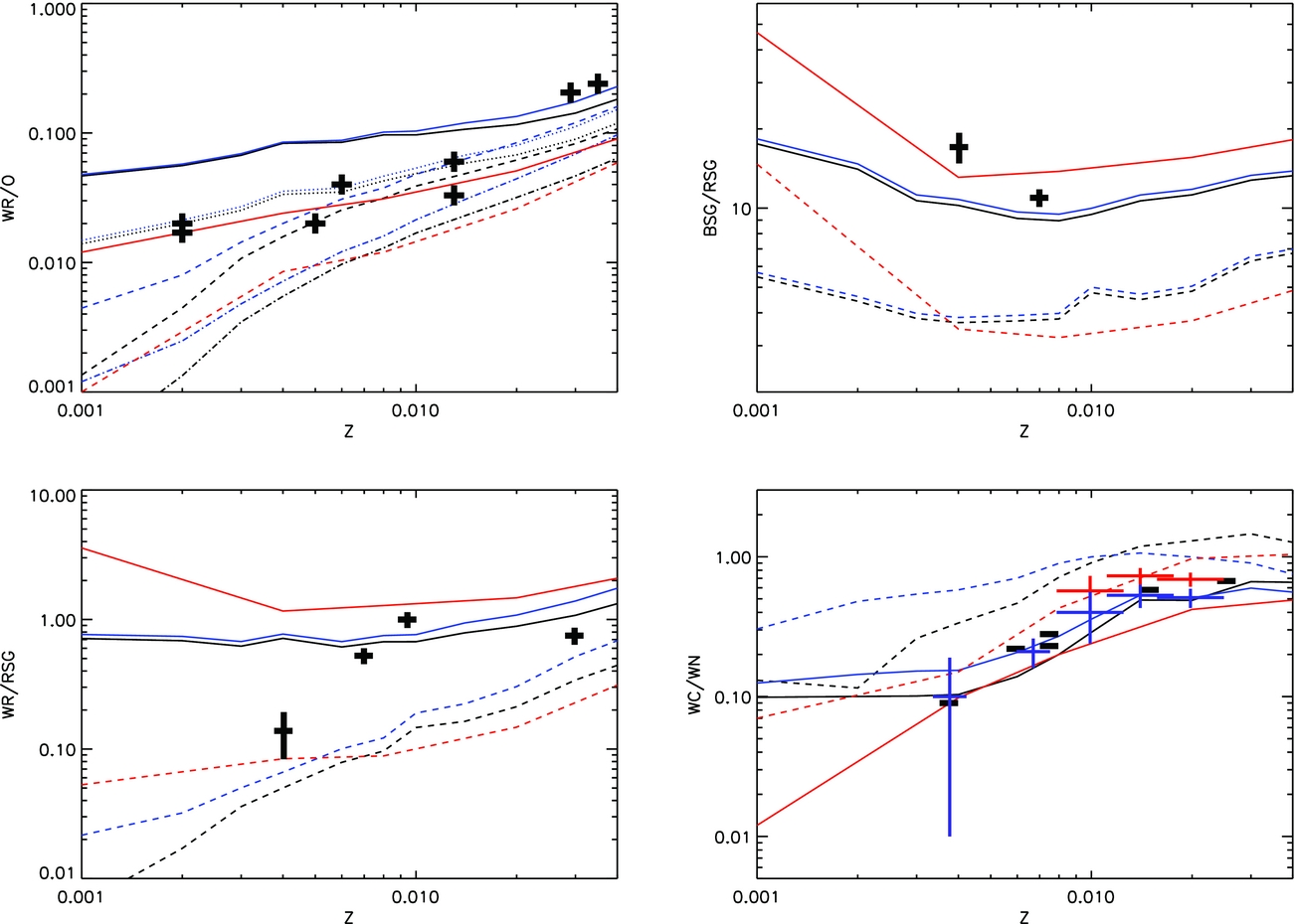
At Solar metallicity, the effect of binaries, and of omitting the lower luminosity O stars, is small. These effects grow at decreasing metallicity, since stars at low metallicity have hotter effective temperatures for the same mass, and thus more O stars are present in the population. Comparison to the observed ratios suggests that models including all main-sequence O stars provide a good agreement to the data, except in the highest metallicity cases. The reason for this is probably related to the fact that the observed sample is old and may suffer from significant incompleteness. Modern, more complete, surveys may find quite different results, but it is encouraging that bpass models reproduce the observed trend in the observed ratios.
The BSG/RSG ratio observational sample (Massey & Olsen Reference Massey and Olsen2003) only contains ratios for the SMC and LMC. Again binary evolution predicts values within a factor of a few of the observed ratios, but somewhat underpredicts the observed BSG fraction, likely due to the lack of rotational mixing in our models. More rotational mixing would lead to more BSGs (Castro et al. Reference Castro, Fossati, Langer, Simón-Díaz, Schneider and Izzard2014) and so we would expect their inclusion to boost our predicted ratio in future and consider the fraction in bpass v2.1 to be a lower limit. We note that the mist models (Choi et al. Reference Choi, Dotter, Conroy, Cantiello, Paxton and Johnson2016) predict a higher BSG/RSG ratio than bpass.
The WR/RSG ratio was presented in our first study with the bpass stellar models (Eldridge et al. Reference Eldridge, Izzard and Tout2008). In v1.0, it was our worst fit of the stellar population ratios since the observational data showed a pronounced trend in ratio with metallicity which the models did not reproduce. Here we compare our models to updated observational numbers (P. Massey, private communication). We see that our binary populations are far closer to the new observed ratios which show a significantly weaker trend. The observational data now shows very little variation in population ratio with metallicity above ~0.3 Z⊙, consistent with the ratios in our models. In the bpass v2.1 model population, the ratio continues to remain flat at lower metallicities. In the observational data set, the SMC is an outlier. However, this ratio is based on only 13 WR stars, suggesting a considerable uncertainty in small number statistics, and potential incompleteness. Alternatively, as the observed data point lies between the single star and binary population predictions from bpass, it is possible that in the case of the SMC, the effective binary fraction could be smaller.
Finally, the WC/WN ratio is the focus of our final comparison between stellar populations and is primarily determined by the WR mass-loss rates. In this figure, we show the latest observations from Rosslowe & Crowther (Reference Rosslowe and Crowther2015) as well as the older sample from Meynet & Maeder (Reference Meynet and Maeder2005). In Eldridge et al. (Reference Eldridge, Izzard and Tout2008), we found that bpass binary WC/WN ratio predictions lay below what was then thought to be the observed ratio. Vanbeveren, Van Bever, & Belkus (Reference Vanbeveren, Van Bever and Belkus2007) discussed in detail how binary populations affect this ratio: binary interactions produce WR stars from low-mass stars which would not otherwise evolve into the WR phase in the single star evolution case. The products of such evolutionary pathways tend to be WN stars rather than WC stars and hence more interacting binaries in a model set causes a drop in the WC/WN ratio. Recent observational surveys presented here show that the ratio is indeed lower than previously thought, in closer agreement to the binary populations predictions. The excellent agreement shown in the bottom right panel of Figure 16 is strong circumstantial evidence that binary interactions are responsible for a good number of WR stars and that single-star stellar winds are not strong enough to create every WR star we see in the sky.
In summary, our population models are consistent with the observed location of post-main sequence massive stars on the HR diagram, as well as the relative numbers of stars we see in galactic stellar populations. This is important as RSG and WR stars have unique spectral signatures in the emergent spectrum from a stellar population. RSGs dominate the longer redder wavelengths, while WR stars are bright in the UV, produce hard ionising radiation, and also strong broad stellar emission lines. The ability of our models to reproduce the stars in resolved populations is good evidence that we likely predict these spectral features accurately.
3.3. Stellar remnants
Compact stellar remnants are the end states of virtually all stars. Since their formation depends primarily on core mass and composition at the end of nuclear burning, their populations can be affected by binary interactions during and after the main sequence lifetime of their progenitors. Thus, the white dwarfs, neutron stars, and black holes in a stellar population present a test of models such as bpass.
The best extant observational data on remnants is on white dwarfs where observers have been able to calculate the observed mass of the white dwarf as well as its initial mass. This is only possible when the white dwarf is part of a stellar cluster from which the age can be estimated, together with the elapsed cooling time of the white dwarf since it was formed. This provides an opportunity to test our initial to final mass relation against these observations. We show in Figure 17 the observed relations (Ferrario et al. Reference Ferrario, Wickramasinghe, Liebert and Williams2005; Kalirai et al. Reference Kalirai, Saul Davis, Richer, Bergeron, Catelan, Hansen and Rich2009) compared to our model predictions at two metallicities.
Initial to final mass relations for compact remnants at two metallicities in the bpass models. The solid central line is the mean remnant mass for that initial mass, dashed lines are the 1 σ lines and the upper solid line is the maximum remnant mass for that initial mass. This can exceed the initial mass due to binary interaction. The left and central panel show white-dwarf data from Ferrario et al. (Reference Ferrario, Wickramasinghe, Liebert and Williams2005) and Kalirai et al. (Reference Kalirai, Saul Davis, Richer, Bergeron, Catelan, Hansen and Rich2009) with the two panels scaled to show different mass ranges for clarity. The horizontal lines indicate the 1.4 and 3.0 M⊙ limiting masses above which we presume neutron stars and black holes to form, respectively. The right-hand panels show the cumulative distribution of observed masses for compact remnants, i.e. the known population sorted by mass and plotted against an arbitrary index number. These are derived from gravitational microlensing within the Galaxy (black, Wyrzykowski et al. Reference Wyrzykowski2016), the observed mass of black holes in X-ray binaries (blue, compiled by Crowther et al. Reference Crowther, Barnard, Carpano, Clark, Dhillon and Pollock2010) and the 10 black holes identified as the sources in candidate gravitational wave transients to date (red, Abbott et al. Reference Abbott2016b, Reference Abbotta, Reference Abbott2017; The LIGO Scientific Collaboration et al. 2017). These demonstrate the range of observed final masses, but their initial masses are unconstrained.
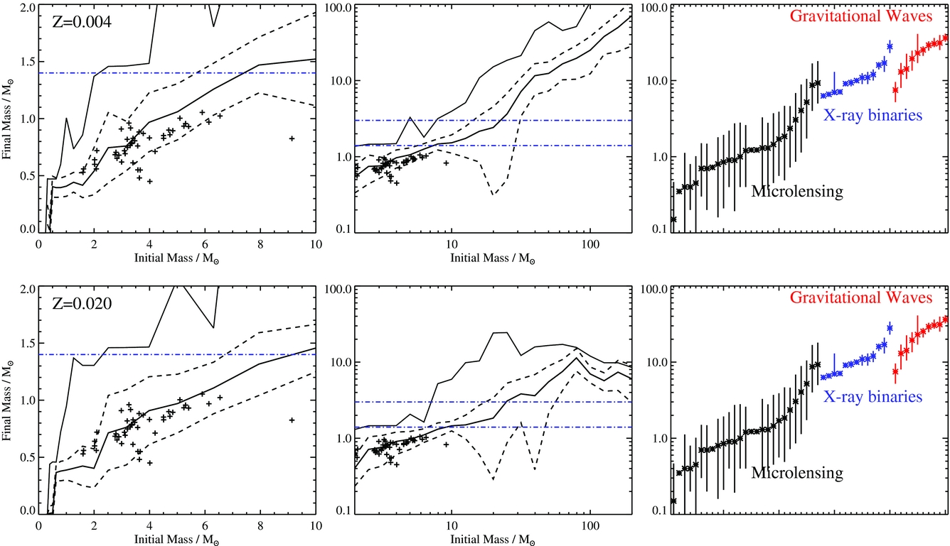
It is important to stress that with the introduction of binary models, the relation between these two parameters is no longer single-valued, there is now a range of possible final masses for any given initial mass. This may naturally explain some of the scatter that is seen in the relation in observed datasets—a result that is difficult to explain in the absence of binary interactions.
The final to initial mass relation for neutron stars and black holes is more difficult to estimate both observationally and in population synthesis models. As yet no black hole has been convincingly associated with a specific initial mass. This may be possible in future if one or more black hole binaries are located in co-eval stellar clusters of a known age, but has yet to be achieved observationally. In Figure 18, instead we compare the range of remnant masses to three different observed data sets: the sample of Wyrzykowski et al. (Reference Wyrzykowski2016) from gravitational microlensing within the Galaxy, the observed mass of black holes in X-ray binaries (compiled by Crowther et al. Reference Crowther, Barnard, Carpano, Clark, Dhillon and Pollock2010), and last, the 10 black holes identified as the sources in gravitational wave transients to date (Abbott et al. Reference Abbott2016b, Reference Abbotta, Reference Abbott2017; The LIGO Scientific Collaboration et al. 2017). This sample remains too small to statistically recover the observed mass distribution, but it does provide constraints on the range of masses for black holes which can compared to the range of final masses in our models. As discussed in Eldridge & Stanway (Reference Eldridge and Stanway2016), formation of the most massive black holes requires very low metallicity stellar populations.
The predicted masses and merger rate for black hole binaries as a function of metallicity, assuming continuous star formation at a rate of 3 M⊙ yr−1 over a 10-Gyr period. The primary is defined as the more massive star at formation (rather than merger). The masses of the black hole progenitors of the five detected gravitational wave transients (four confirmed events, one lower significance candidate) are indicated (LIGO Scientific Collaboration et al. 2015; Abbott et al. Reference Abbott2016b, Reference Abbotta, Reference Abbott2017; The LIGO Scientific Collaboration et al. 2017)—each appears twice depending on the evolutionary history. Lines indicate mass ratios of unity, 0.5 and 2.0.

Compact object binaries lose energy through gravitational radiation. As a result, the binary orbit hardens until eventually the compact objects come into contact and merge, emitting a gravitational wave transient in the process. We have looked at the merger times of compact remnant mergers, and made predictions based on our baseline v2.0 models, in Eldridge & Stanway (Reference Eldridge and Stanway2016). Our rough volume average rate estimate for neutron star–neutron star mergers is 210 to 1 600 Gpc−3 yr−1, for black hole–neutron star mergers 0.07 to 62 Gpc−3 yr−1, and for black hole to black hole mergers 8 to 120 Gpc−3 yr−1. These predictions are compared against the gravitational wave transients reported to date in Figure 18—all five events are consistent with emerging from environments at <0.5 Z⊙, with the two most massive events most likely arising at significantly lower metallicities, in good agreement with our earlier work. Interestingly, all events are consistent with a final mass ratio <2, suggesting that the parameter space for detectable mergers may be a little narrower than the population in our models. We note here that a number of uncertainties remain in making such predictions. Key amongst these are the remnant lifetimes and merger timescales. These are dependent on uncertainties such as supernova kicks, the resulting orbital eccentricity and CEE, all of which introduce associated uncertainty into predictions of event rates, even if the age distribution and star formation history of potential sources are known. As discussed in Section 7.7, we are currently investigating a new model for supernova kicks (Bray & Eldridge Reference Bray and Eldridge2016) but this is still largely unconstrained by observations. Until we have a stronger constraint on the distribution of such kicks, and a larger observational sample for comparison and verification, we choose not to refine our predictions further here.
4 SUPERNOVAE AND TRANSIENTS
Massive stars can be defined as those that end their lives in a core-collapse supernova. Here we outline some of the outputs from our populations that concern supernovae; namely, the delay time distribution, the relative rates and the predicted location of SN progenitors on the HR diagram.
In Figure 19, we show the delay time distribution for different core-collapse event types for our single star and binary populations at two different metallicities. We compare our predictions to observed delay-time distributions in a similar method to that performed by Zapartas et al. (Reference Zapartas2017). The left-hand panels show the predictions for single star populations. We see that, at Solar metallicity, the oldest supernovae occur at stellar population ages no older than 80 Myrs, and there is a clear progression of supernova types from Ic to Ib, then II and IIP. At lower metallicity, this sequence is less clearly defined.
Supernova rate distributions with stellar population age. In the left-hand panels, we show single star models at two metallicities, while in the central panels we show the equivalent rates for a binary population. The right-hand panels consider the total supernova rate (including type Ia events, black) with the solid line giving binary models and the dotted single star models. The triangle points are the observed core-collapse supernova rates reported by Maoz & Badenes (Reference Maoz and Badenes2010). The data points indicate type Ia SN rates from Maoz, Sharon, & Gal-Yam (Reference Maoz, Sharon and Gal-Yam2010, crosses) and Totani et al. (Reference Totani, Morokuma, Oda, Doi and Yasuda2008, squares).
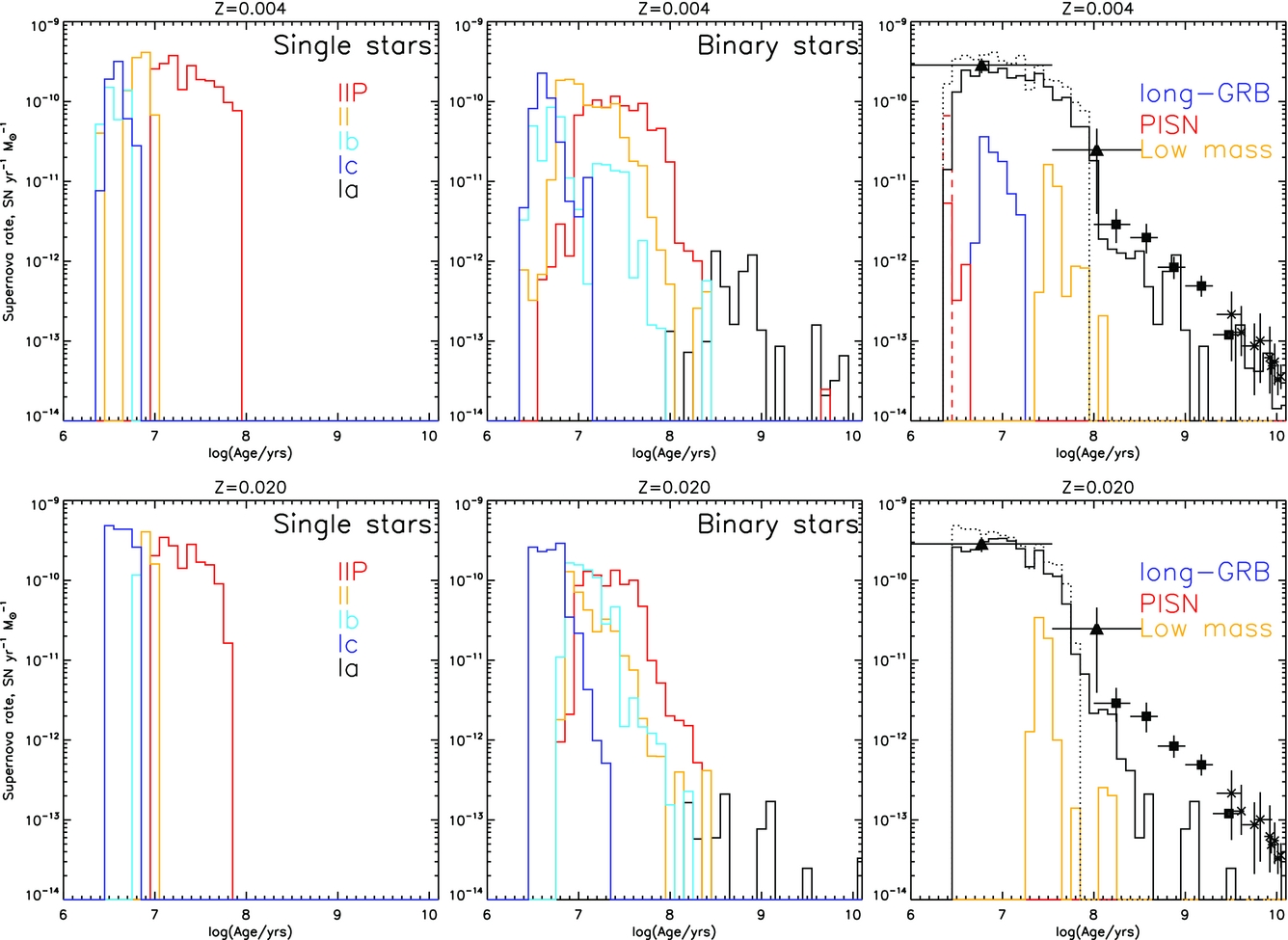
We consider binary populations in the central panels of Figure 19. With the presence of binaries, the core-collapse SNe extend over a much broader rate of ages, continuing to occur up to a stellar population age of a few times 100 Myrs. This is a common prediction from binary population synthesis as recently highlighted by Zapartas et al. (Reference Zapartas2017). There is still a general trend of SN types from Ic, Ib, II to IIP at both metallicities, but there is also now much more overlap. This is due to the existence of a variety of evolutionary pathways with different strengths of interactions, rather than a single pathway for each stellar mass. The binary predictions also show estimates for type Ia SNe, which become possible at late times as core-collapse SNe decline. The rate of type Ia events increases as the metallicity of the stellar population drops below Solar in our models. There may be some observational support for this; Quimby et al. (Reference Quimby, Yuan, Akerlof, Wheeler and Warren2012) identified a tendency for white dwarfs to be observed more commonly in low luminosity dwarf host galaxies, which tend to be sub-Solar in metallicity in the local Universe. We stress again that our type Ia rates are currently highly approximate and do not include much of the detailed physics required (see Section 2.1.3). However, it is encouraging that our estimated delay times for these event are consistent with when other population synthesis models suggest they should occur (Maoz, Mannucci, & Nelemans Reference Maoz, Mannucci and Nelemans2014, and references therein).
The final pair of panels in Figure 19 (right) show rarer transient event types. They indicate that PISN and long-GRBs form by pathways considered in bpass only occur at low metallicities and at the younger ages. It should be noted that our long-GRB rates represent a lower limit since there are certainly higher metallicity pathways to forming GRBs, which are seen up to Solar metallicity. These events likely appear in our models as a subset of the type Ic supernovae. We also show where low-mass type explosions may occur. These sources have progenitors between 1.5 and 2.0 M⊙—the observational appearance of any transient resulting from these remains uncertain (Moriya & Eldridge Reference Moriya and Eldridge2016). However, we have included them for completeness and we note that their total rate is low relative to core-collapse, or even type Ia events. Future work will attempt to simulate explosions in these stellar models, yielding a better idea of whether they should be included in the population synthesis of SN rates.
We now take the total number of core-collapse SNe arising over the first 10 Gyr after the formation of 106 M⊙ of stars at each metallicity, and compare them in Figure 20. We see the expected trend with metallicity as a consequence of the metal dependence of stellar winds driving mass loss. For example, there are more IIP SN at lower metallicity at the expense of the type Ib and Ic SNe, since fewer stars lose their hydrogen envelope before supernova. We also see the rate of type Ia SNe increasing at lower metallicity for the same reason. Binary interactions weaken this trend by providing alternate mechanisms for mass loss at lowest metallicities, but do not remove it.
Total number of supernovae arising from a 106 M⊙ stellar population within 10 Gyr of its formation, shown as a function of metallicity. Solid lines indicate binary populations, while dashed lines give equivalent single star populations.
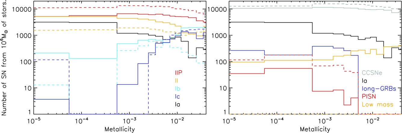
Our predicted long-GRB and PISN rates are relatively stable below a metallicity of Z = 0.004, at which they start to occur. Our predicted rates are, of course, subject to uncertainties, for example, whether we include the low-mass events in our sample, or whether we include SNe where a black hole is formed rather than a neutron star remnant since for some of these the explosion may be concealed within the event horizon. Graur et al. (Reference Graur, Bianco, Huang, Modjaz, Shivvers, Filippenko, Li and Eldridge2017) compared our predicted ratios of type Ib/c and II SNe to the observed SN type ratios and found good agreement. However, we caution that relative rates determined from observations are still somewhat dependent on sample completeness and observational bias and often have poor metallicity constraints.
We can also test our models by considering the observed progenitors of SNe. If an SN occurs within about 20 to 30 Mpcs of the Sun, and the host galaxy has been imaged by the Hubble Space Telescope before the transient event, there is a very good chance that the progenitor star could be detected in a pre-explosion image. We show in Figure 21 the observed locations in the HR diagram for a sample of well-constrained progenitors, as well as the predictions from our stellar models as to where the SN should be. Here the underlying greyscale contour map represents the locations of all supernova events expected in a stellar population with our IMF regardless of type and when they occur, while the line contours on each panel select only those expected to produce a given SN subtype. For the observed datapoints, use the sample of Smartt (Reference Smartt2015) supplemented by SNe 1987A (Walborn et al. Reference Walborn, Lasker, Laidler and Chu1987) and 1993J (Aldering, Humphreys, & Richmond Reference Aldering, Humphreys and Richmond1994), as well as the recent ‘failed supernova’ event in NGC 6946 (Adams et al. Reference Adams, Kochanek, Gerke and Stanek2017).
Prediction of the final location of SN progenitors on the HR diagram. The blue asterisk is the RSG that vanished (i.e. the candidate black hole formation event Adams et al. Reference Adams, Kochanek, Gerke and Stanek2017), diamonds indicate pre-explosion upper limits on luminosity from (Smartt Reference Smartt2015), the X in the IIP panel is the progenitor of SN1987A (Walborn et al. Reference Walborn, Lasker, Laidler and Chu1987), and in the IIb panel is SN1993J (Aldering et al. Reference Aldering, Humphreys and Richmond1994). Underlying greyscale contours give the total core-collapse SN progenitor distribution from a 106 M⊙ stellar population given our assumed IMF, while overlying line contours indicate expected progenitors for each subclass. We average the populations from Z = 0.008 to 0.020 to allow for metallicity spread in the observational data.

As Figure 21 shows, type IIP progenitor stars are both predicted to be and observed to be primarily RSGs. The one exception is the progenitor of SN1987A which is a BSG. The type IIb SN progenitors detected to date all appear to be YSGs or RSGs. Here there is overlap with our models but it is interesting that we also predict some progenitors that should be substantially hotter than we have observed to date. When the hydrogen envelope drops below about 1 M⊙ in mass, the surface temperature in our models can change rapidly for small amounts of further mass loss and so is very sensitive to time step and exact conditions. The discrepency between models and observations for these stars may thus arise from the difficulty of predicting the correct surface temperature. Our models favour BSG or RSG rather than YSG progenitors.
For the type Ib/c SNe, only one progenitor has been observed, iPTF13bvn (Cao et al. Reference Cao2013; Eldridge & Maund Reference Eldridge and Maund2016). As described by Eldridge et al. (Reference Eldridge, Fraser, Smartt, Maund and Crockett2013), we also have a large number of non-detections consistent with the prediction that the progenitors are all hot and faint in the optical (although UV-bright). The Ib progenitors while fainter than those of type Ic events, are cooler and thus brighter optically and so were the first to be observed (as predicted by Yoon et al. Reference Yoon, Gräfener, Vink, Kozyreva and Izzard2012).
Finally, we note that the progenitor of the only-known candidate black hole forming event (Adams et al. Reference Adams, Kochanek, Gerke and Stanek2017) was identified through the disappearance of a luminous star in the well-studied galaxy NGC 6946. This star was expected to go supernova and thus it has been suggested that any explosion energy was contained within the event horizon of a forming black hole at the star’s core. The progenitor star was the most luminous RSG in the sample which fits with our understanding that more massive RSGs should form black holes and not have visible supernovae. This provides a test of our prescriptions for when black holes are formed as remnants within our model set.
5 SPECTRAL SYNTHESIS VALIDATION: RESOLVED AND UNRESOLVED STELLAR POPULATIONS
Population synthesis models such as ours are used to interpret the integrated spectral appearance of unresolved stellar populations. However, both stellar binaries and resolved stellar clusters provide an opportunity to explore the colours and spectral properties of individual stars within the context of a co-eval stellar population.
In Figure 22, we revisit the sample of eclipsing binaries discussed in Section 3. We compare the B − V colours of these sources to the synthetic colours predicted by our spectral synthesis models. The observed colours are broadly consistent with the expected behaviour in both temperature and mass for these well-constrained systems, with the models successfully reproducing the stellar main sequence and also accounting for much of the scatter in colour at intermediate masses. There are, however, a few notable failures. In particular, the highest mass system in the observed sample (WR20a) shows colours considerably redder than predicted for its temperature and mass, while other massive stars are also a few tenths of a magnitude redder than might be expected. This likely reflects the fact that massive stars are typically found in young star-forming regions behind large amounts of dust. In fact, WR20a is at distance of nearly 8 kpc towards the Galactic centre and thus the colours are significantly reddened. Lower mass stars are typically in older regions with less dust attenuation, so it is unsurprising that these show better agreement with our models.
The eclipsing binary star sample presented in Figure 9, but now showing the B − V colour of the binary versus both the mass and surface temperature of the primary star. Observational data points are colour coded by mass, while the underlying contours indicate the parameter space accessed by the same binary population as in Figure 9.
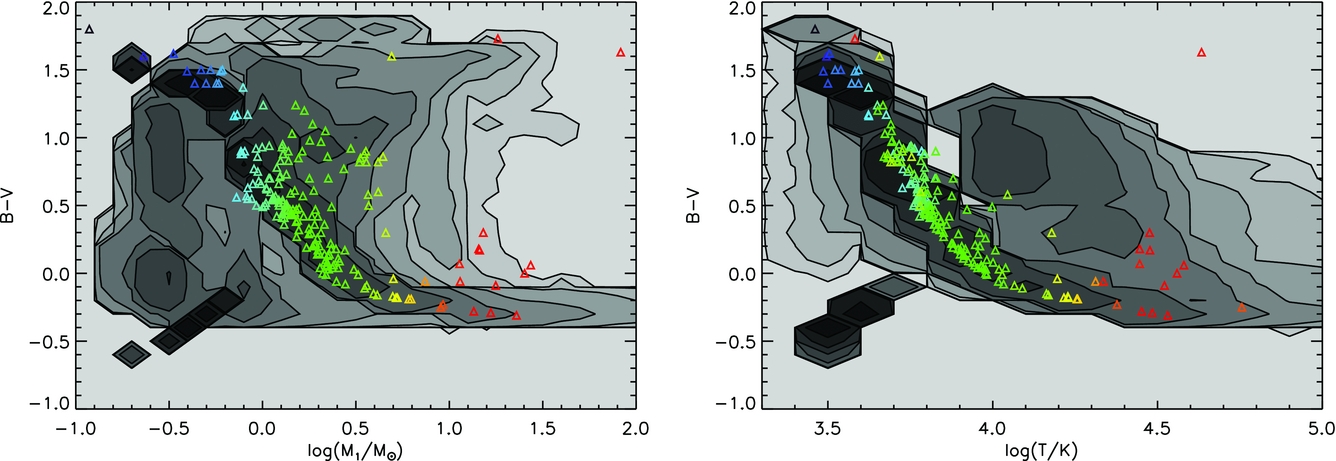
In Figures 23 and 24, we compare the theoretical HR diagrams and the observational cCMDs for the same three clusters. Any incompatibility between our population synthesis (based on evolutionary models) and spectral synthesis (which combines these with atmosphere models) should be revealed by the comparison. Age estimates for each cluster are based on a determination by eye and by comparing to earlier literature of the ages of the clusters. We typically use the binary star models. Fits by single-star populations are also possible if blue-straggler stars are ignored.
Comparison of predictions of the HR diagrams for the clusters Cygnus OB2 (top), Upper Scorpius (middle) and NGC6067 (lower, spectroscopic HR diagram) and the location of observed stars in these clusters. The left panels are for single-star population and the right-hand panels include interacting binaries. The ages are chosen such that the binary star population has qualitatively the best fit.
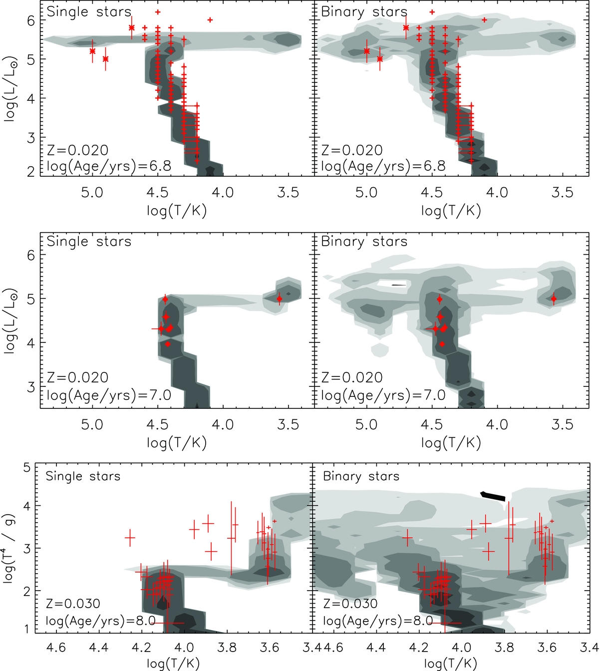
Comparison of predictions of stellar locations on the CMDs for the clusters Cygnus OB2, Upper Scorpius, and NGC6067.
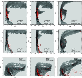
The Cygnus OB2 association (Wright, Drew, & Mohr-Smith Reference Wright, Drew and Mohr-Smith2015) and Upper Scorpius (Pecaut, Mamajek, & Bubar Reference Pecaut, Mamajek and Bubar2012) are best fit in our models at stellar population ages log(age/yrs) = 6.8 and 7.0, respectively, while NGC 6067 (Alonso-Santiago et al. Reference Alonso-Santiago, Negueruela, Marco, Tabernero, González-Fernández and Castro2017) is fit at log(age/yrs) = 8.0. This age for Cygnus OB2 is at the higher end of the range suggested by previous studies, as we would expect with a binary population. For Upper Sco, the strongest constraint is given by the existence of Antares, and this fixes our models to an approximate age of 10 Myr, very similar to the 11 Myr found by Pecaut et al. (Reference Pecaut, Mamajek and Bubar2012). Our age for NGC 6067 agrees with previous estimates. The HR diagrams for single star models are presented on the left of Figure 23 and binaries on the right. Interacting binaries broaden the range of properties (and hence colours) expected for cluster members. If we used single star models for these comparisons, we would have to use a much younger population to fit the bulk of stars, but we would not be able to match the luminosity of the WR stars. The binary population spreads out the most luminous stars significantly in temperature at late ages. In older clusters, blue stragglers typically form a very clear group above the main-sequence turn-off; in younger clusters, it is difficult to separate these out and identify the true, non-interacting, main-sequence stars. CMDs for these clusters extending from the optical to the near-infrared are shown in Figure 24. The stellar main sequences predicted from the HR diagrams are coincident with the location of stars in their CMDs albeit subject to some uncertainties in extinction effects (which may be present in the blue bands, particularly for Upper Sco), providing a verification test for the atmosphere models which dominate in young stellar populations.
In Figure 25, we present CMDs for three additional old stellar clusters, compared to photometric data for cluster members drawn from the WEBDA databaseFootnote 7 . In each case, the appropriate age has been drawn from our models by eye for comparison. We estimate log(age/yrs) of 7.9, 8.6, and 9.1 for IC2602, NGC3532, and NGC752, respectively. These compare to log(age/yrs) of 7.5, 8.5, and 9.05 from the WEBDA database. Again a single star (at the top of the main sequence) drives the fit for IC2602, and the existence of this star is possible at an older age in BPASS models than in typical single star models since binary models permit the existence of blue stragglers.
Colour–magnitude diagrams for three additional old stellar clusters, IC2602, NGC3532, and NGC752, compared to photometric data drawn from the WEBDA database (see text). In each case, the approximate age has been estimated.

As the figure demonstrates, bpass binary models simultaneously reproduce the locations in colour–magnitude space of the main sequence and red giant branch for these clusters. While some scatter remains which cannot be explained by binaries, we cannot rule out the presence of non-cluster interlopers in the available available catalogue data particularly at faint absolute magnitudes.
A final strong test of simple stellar populations can be obtained by comparing the colours derived from our models to those of unresolved but (likely) single-aged stellar clusters in a nearby galaxy. In Figure 26, we do so, making use of the M33 star cluster population identified by San Roman, Sarajedini, & Aparicio (Reference San Roman, Sarajedini and Aparicio2010). The colour of an unresolved population evolves rapidly in the first ~10 Myr after the onset of star formation and thereafter more slowly, and with relatively little dependence on stellar metallicity. In Figure 26, we do not plot tracks with ages <5 Myr since these are likely to be severely affected by nebular emission and potentially enshrouded by natal dust clouds. With the exception of the youngest sources then, bpass models appear to qualitatively reproduce the range of colours observed in the star clusters of M33, particularly if moderate reddening (with E(B − V) up to 1) is permitted.
The photometric colours of unresolved star clusters in the M33 system, overplotted with evolution tracks at four different metallicities. Solid lines show the evolution with age of bpass models for a single-aged starburst from 5 Myr (bluest colours) to 1 Gyr. Dashed lines indicate the same but for a population continuously forming stars at a constant rate of 1 M⊙ yr−1. The thick lines indicate a population without dust reddening, while the offset tracks shown in thin lines have a dust extinction of E(B − V) = 1, assuming the Calzetti dust law. Data points are drawn from the photometric catalogue of San Roman et al. (Reference San Roman, Sarajedini and Aparicio2010) and include only their ‘highly probable’ or ‘confirmed’ clusters with m g < 19.5.

In summary, by testing our evolution models against observational data on Hertzsprung–Russell diagrams, their respective CMDs and colour–colour diagrams, we have shown that the evolutionary models and atmosphere models can be used with confidence, especially when studying unresolved clusters.
6 COMPLEX STELLAR POPULATIONS
By their nature, the integrated light from most galaxies is challenging to simulate. The stellar component of a galaxy typically consists of a number of low mass individual stellar populations, not necessarily co-eval and each embedded in the interstellar medium. Their light is modified by the interstellar gas and by scattering, absorption and re-emission from dust grains. Nonetheless, the underlying spectral energy distribution of a galaxy, together with the gas excitation and dust temperature, is fundamentally shaped by its stellar population. The nebular continuum and emission lines are primarily driven by Lyman continuum photons and hence by the youngest stars. Thus, the interpretation of integrated light from galaxies is also largely dependent on stellar population synthesis models and the range of observed galaxy properties provides a constraint on those models. Here we present observational constraints on the performance of our models in galaxy-scale stellar systems.
6.1. Wolf–Rayet galaxies
A straightforward observational verification test of our bpass models in extragalactic stellar populations is provided by so called ‘WR’ galaxies, classified through strong emission in regions of the spectrum in which the WR stars provide the dominant flux contribution, primarily centred on the He ii 4 686 Å line (the ‘WR blue bump’) and C IV5808Å (the ‘WR red bump’). The presence of these massive, stripped-envelope stars is taken to indicate a recent, massive starburst which should thus be possible to match against our single-age starburst models.
Observational samples of WR-dominated stellar populations, particularly those with follow-up spectroscopy, have improved since we presented an initial analysis of these systems with our v1.0 model set (Eldridge & Stanway Reference Eldridge and Stanway2009). López-Sánchez & Esteban (Reference López-Sánchez and Esteban2008, Reference López-Sánchez and Esteban2010a, Reference López-Sánchez and Esteban2010b) analysed a sample 20 nearby WR galaxies, determining the photometric colours of both the integrated galaxy and distinct star-forming regions within it. In Figure 27, we compare the predictions of our models to the photometric colours measured for that sample. We omit the photometry for underlying stellar populations (which are typically old) and for companion galaxies and compare against data for which an estimated nebular gas emission component has previously been subtracted. Given the photometric scatter in the data, the observed colours of WR-dominated star-forming regions are consistent with both single and binary star models. Although neither set of tracks precisely reproduces the data, the observations are arguably more consistent with our binary models than our single star models, particularly in Johnson B − V − R colour space, although they tend to be ~0.2 mag redder in B − V than binary tracks, perhaps suggesting that the nebular contribution to the B band has been over-estimated. Unfortunately, the broad band colours are only weakly sensitive to metallicity and the uncertainties on the photometric data do not allow a more quantitative study of this sample.
The photometric colours (in the Johnson–Vega system) for measured star-forming regions in the López-Sánchez & Esteban (Reference López-Sánchez and Esteban2008) sample of Wolf–Rayet galaxies. Tracks show the evolution in colour with age for single-age starbursts comprised of single stars (dashed) and binary stars (solid lines), at three different metallicities. The catalogue photometry was adjusted by López-Sánchez & Esteban to remove an estimated nebular contribution (typically Δmag ~ 0.05 − 0.10) and is compared to stellar tracks without nebular emission. The median photometric uncertainties of the datapoints in each colour is indicated in the lower right of each panel.
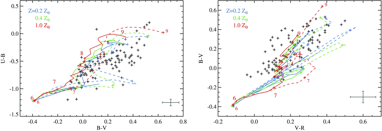
To assess our model predictions for the strength of the WR stellar features in the spectra of galaxies or their resolved star-forming regions, we supplement the López-Sánchez & Esteban (Reference López-Sánchez and Esteban2010a) spectroscopic sample with two further studies. The first, presented here for comparison with our own earlier work is the Brinchmann et al. (Reference Brinchmann, Pettini and Charlot2008) sample of WR galaxies selected from SDSS. These were selected through use of a virtual narrowband filter to identify archival spectra with a flux excess at the expected wavelengths, before the broad spectral lines were individually measured. The second is a sample selected for spectroscopic follow-up by Sokal et al. (Reference Sokal, Johnson, Indebetouw and Massey2016) as individual WR-hosting star clusters in six nearby galaxies. In common with the López-Sánchez & Esteban (Reference López-Sánchez and Esteban2010a) selection, while the galaxies themselves are resolved, the individual star forming regions are not. In each of the samples discussed here, the original authors corrected their spectra for an inferred nebular flux contamination and determined a metallicity (either from the ‘direct temperature’ or through empirical strong line indicator methods), before estimating the flux or equivalent width in the WR red and blue bumps.
bpass stellar population models have evolved since the early results were presented in Eldridge & Stanway (Reference Eldridge and Stanway2009). We predict comparable blue bump equivalent widths from binary populations to our earlier models at twice Solar metallicity. Our predictions at lower metallicities have risen from ~0.5 Å (at 0.05 Z⊙) to almost 4 Å. Our predictions for single star models have also changed, with the new populations generating less emission in the blue bump at late ages than the earlier models (primarily due to an improved treatment of O- and Of-stars). Similarly, our new models predict stronger emission in the red bump than before, particularly at low metallicities and early times. Interestingly, we see a strong metallicity dependence on the line strengths in both WR features. Both bumps show two peaks in line production with stellar population age, one at ~3 Myr and attributable primarily to the ionising flux from short-lived massive WO stars, and the second at ~10 Myr due to formation of late-WN and WC stars. Evolution into these stellar classes, and the ratio between them, is strongly dependent on metallicity (see McClelland & Eldridge Reference McClelland and Eldridge2016). At low metallicities, the WC phase is never reached as a result of low mass loss rates, the surviving WN stars remain luminous in the Helium-dominated blue bump, but do not contribute strongly to the carbon-dominated red bump. At high metallicities, WC stars form and thus a strong peak is seen in the red bump at late times.
The v2.1 models do well at recovering the broad distribution of spectroscopic properties, with models at near-Solar metallicity and ages of ~3–10 Myr simultaneously reproducing the observed strengths of both WR bumps in most cases. Having said that, the comparison is not without tension. Younger ages are preferred by fits to the blue bump as opposed to slightly older ages in the red bump. There are also a number of sources for which none of our single-age, single metallicity models reproduce the observed lines, these are found predominantly in the Brinchmann et al. (Reference Brinchmann, Pettini and Charlot2008) sample. Unlike the other two samples shown in Figure 28, in which individual star-forming regions have been identified (if not resolved), this sample comprises entirely unresolved galaxies. The nebular correction for these sources, as well as the underlying old stellar continuum, has been determined by comparison with earlier population synthesis models and so is somewhat dependent both on the stellar models in that code (which did not incorporate binary interactions or rotation) and the presumed star-formation history. Given the extremely prominent red and blue bumps in this sample, and their inconsistency with both the semi-resolved samples and our single age starburst models, two possibilities present themselves: the nebular contribution may have been underestimated in the catalogue correction (i.e. approximately one-third of the reported line flux has a nebular emission origin), or there is a significant contribution from diffuse interstellar medium between individual star-forming regions. The latter appears unlikely, given the high ionisation potentials required to excite the emission lines dominating each bump.
The predicted strengths of the Wolf–Rayet ‘red’ and ‘blue’ bumps, centred on He ii 4 686 Å and C iv 5 808 Å, respectively. All line strengths are given as equivalent widths in angstroms, with positive values indicating emission. Tracks show the evolution in colour with age for single-age starbursts comprised of single stars (dashed) and binary stars (solid lines). The top panels show the time evolution of the line strengths as a function of metallicity. The centre panels compare the strengths of starbursts of equal ages (labelled as log(age/years) in the upper left) at different metallicities. These are compared with the combined catalogue data of López-Sánchez & Esteban (Reference López-Sánchez and Esteban2010a, LE10), Sokal et al. (Reference Sokal, Johnson, Indebetouw and Massey2016, S16), and Brinchmann et al. (Reference Brinchmann, Pettini and Charlot2008, B08) in grey scale, with dark regions indicating a higher density of sources. Catalogue photometry was adjusted by the original authors to remove estimated nebular contribution and is compared to stellar tracks without nebular emission. In the bottom panels, the strengths of the two bumps are compared simultaneously with tracks at equal age (left) or metallicity (right). Note that model agreement is far better with the LE10 and S16 data than that of B08.

6.2. Star-formation history
The default bpass models produce the stellar output spectrum for a burst of stars formed at a given time before present. From these, it is possible, and often necessary, to construct integrated spectra representing more complex star-formation histories such as exponentially rising or falling, or multiple burst histories. Inevitably, this results in the addition of free parameters describing this history, in addition to those associated with the stellar models. Our preferred approach therefore is to explore as limiting cases the evolution of an instantaneous, rapid burst of star formation and of a continuous moderate (1 M⊙ yr−1) star-formation episode as a function of time, while noting that neither case may be appropriate to any given galaxy.
We present an illustration of the resulting uncertainties in Figure 29. The figure indicates the time evolution of the ionising flux from stellar populations which either peak at the same star-formation rate (left-hand panels) or produce the same total mass of stars (right-hand panels), but which display a range of star-formation histories and either neglect (upper panels) or incorporate (lower panels) the effects of binary evolution. The models shown are at a metallicity of 0.1 Z⊙ since the effects discussed are strongest at lower metallicities and weakest around Solar metallicity. The clearest, most distinctive difference is that the binary population incorporates a higher fraction of hot stars, and so produces higher fluxes at a fixed star-formation rate. However, careful inspection reveals a second, also significant factor which is partly obscured by the necessity for logarithmic scaling in the figure. Populations incorporating binaries produce ionising flux for longer and thus the continuous star-formation history does not reach a steady state until later in the binary population starburst, while the more complex star-formation histories also peak somewhat later than in the single star evolution case.
The ionising photon flux (i.e. Lyman continuum emission in photons per second) from a stellar population given five different star-forming histories. Upper panels show the results for our single star models. Lower panels illustrate the same but for a population incorporating binaries. The solid line indicates continuous star formation at a constant rate, the dotted line a single, instantaneous starburst at the onset of star formation. The dashed and dot-dashed lines indicate exponentially decaying star-formation histories in which the rate varies with time as exp(−t/τ), with τ = 100 Myr and 1 Gyr, respectively. The dot–dot-dashed line indicates a ‘delayed exponential’ star-formation history, in which the rate varies as t/τ exp(−t/τ). In the left-hand figure, the maximum star-formation rate is scaled to 1 M⊙ yr−1 (106 M⊙ in stars in the first Myr for the instantaneous burst), while in the right-hand figure, the populations are scaled to produce the same mass, 1010 M⊙ by stellar population age 10 Gyr.
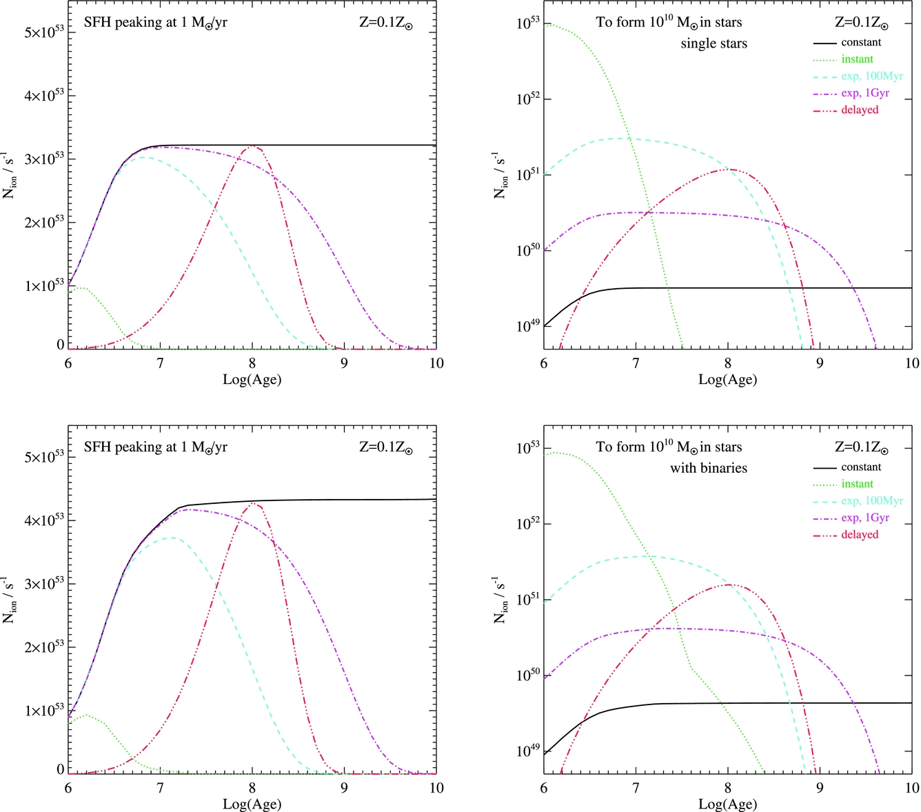
As the figure makes clear, any simple prescription which assumes a fixed conversion from ionising flux, or its proxy Hα line emission in the optical, to an ‘instantaneous’ star-formation rate neglects rather significant uncertainties on the origin of the ionising photons and the past star-formation history, which are increased in a binary stellar evolution scenario due to the range of possible stellar lifetimes for ionising sources. Care will also be required in interpreting the colours of composite stellar populations due to contributions from both nebular continuum and emission line reprocessing of this ionising flux.
A similar stellar lifetime effect is seen in the photometric colours of composite stellar populations. Figure 30 compares the colour evolution of the populations (using the SDSS ugriz filter system and neglecting the effects of nebular continuum, see below). For both single and binary evolution models, the instantaneous starburst shows more stochastic variation in colour, as different mass populations reach the end of their main sequence or post-main-sequence lifetimes and a dramatic colour change appears. In the composite stellar populations, this variation is smoothed out by stars which formed slightly later, reducing the variability in photometric colour of the population. The colour differences between the single and binary models are relatively small (Δ mag~0.1) in the visible bands (gri), and at early ages (~108 yrs). The behaviour with age in the two populations is similar. The binary population is consistently bluer than its single star counterpart with the colour difference most pronounced in the SDSS u − g colour, and at ages >1 Gyr, where the binary models are as much as 0.8 mag bluer than the single star models. It is notable, if unsurprising, that the shortest wavelength of the standard SDSS colours also most clearly shows the impact of the star-formation history, with old instantaneous bursts redder than populations forming stars over a more extended time period. Delayed and exponentially declining starbursts begin their lives approximating the colour of a continuous starburst, before converging with the colours of an instantaneous starburst at a time comparable to their exponential timescales, τ.
The photometric colours (in the SDSS ugriz system) for a stellar population given five different star-forming histories. Left panels show the results for our single star models. Right panels illustrate the same but for a population incorporating binaries. Note that nebular emission is not included (see Figure 31). Star-formation histories are shown defined in Figure 29.
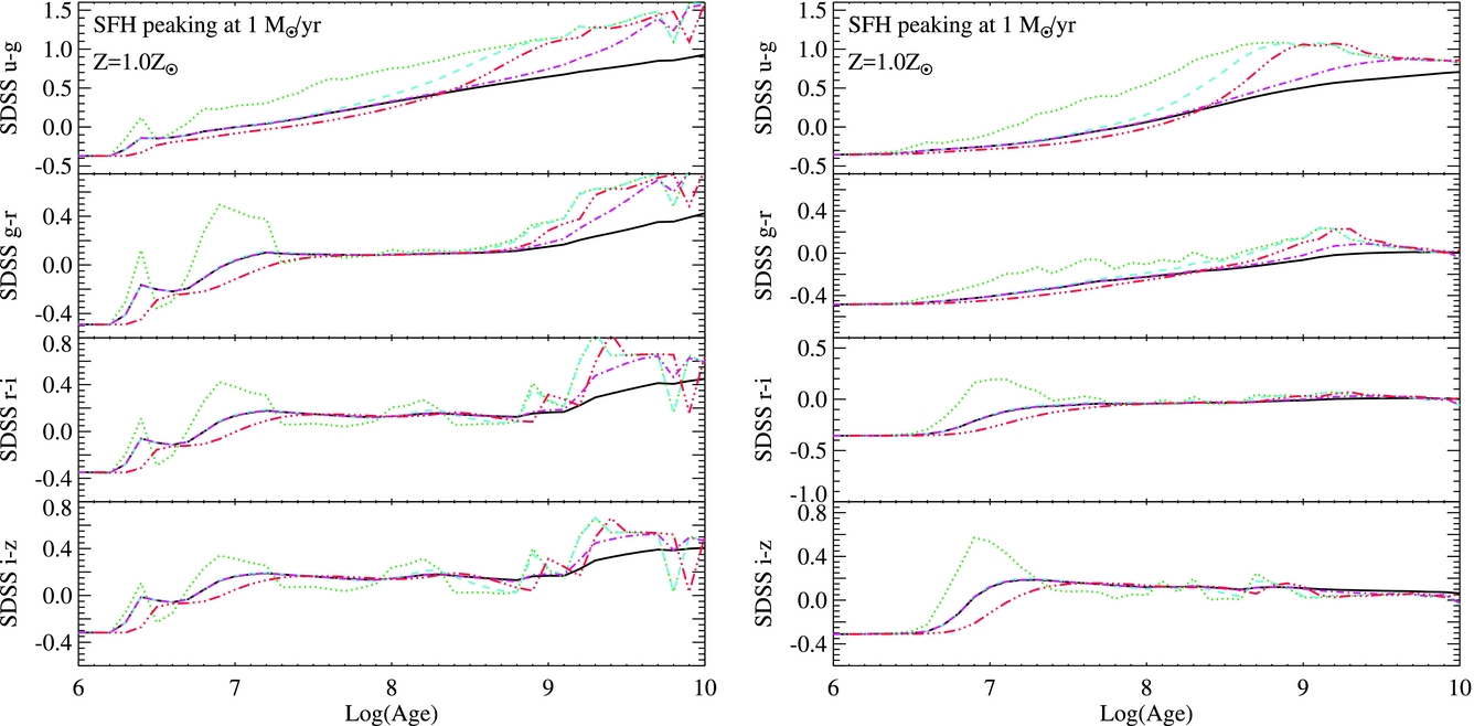
6.3. Nebular emission
The radiative transfer of this stellar emission through nebular gas screen within the source galaxy is beyond the scope of bpass itself, but can be modelled in detail using a radiative transfer code such as cloudy (Ferland et al. Reference Ferland, Korista, Verner, Ferguson, Kingdon and Verner1998) or mappings (see Dopita et al. Reference Dopita, Sutherland, Nicholls, Kewley and Vogt2013, and references therein) to assess the contribution of nebular continuum and line emission. Again, this adds degrees of freedom to any model that attempts to explain observed galaxies, in the form of the interstellar gas density and its geometry, or alternatively in the form of the ionisation parameter. This measures the ratio of the number of ionising photons to the local gas density, and is thus constructed through the combination of appropriate stellar atmosphere models and a choice of gas distribution (e.g. Byler et al. Reference Byler, Dalcanton, Conroy and Johnson2017). As Figure 6 makes clear, however, the extreme ultraviolet is a spectral region severely affected by the presence of absence of binary evolution. These hard photons are seldom observed, but instead reprocessed by the interstellar medium and thus nebular emission cannot be ignored in any complex stellar population.
Detailed comparison with observed extragalactic spectra requires a grid of models with different gas density and geometry since self-shielding and collisional excitation or de-excitation of ions can alter the transition probabilities in either very sparse or very dense gas. Such a grid is explored in Xiao et al. (Reference Xiao2017). Here we present a single model for clarity. Our baseline model for nebular emission is constructed using cloudy v13.03. It assumes an electron density of 102 cm−3, distributed in a sphere around the stellar population. In previous work, we have used a gas distribution with an inner radius of 10 parsec, corresponding to an ionisation parameter of −2.26 for an established population forming stars with a constant rate of 1 M⊙ yr−1 at Z⊙ in our binary models, and −2.59 for our single star models, assuming a typical electron fraction of 10−3. An inner radius of 3 pc yields equivalent ionisation parameters of −1.21 and −1.55.
We assume that the nebular emission is radiation bounded, allowing for absorption through the diffuse interstellar medium between individual star-forming clusters. Our selected gas density is a typical value for extragalactic star forming H ii regions in the local Universe, although we note that these range over several orders of magnitude in density (see e.g. Hunt & Hirashita Reference Hunt and Hirashita2009), and there are indications that a slightly higher nebular gas density ~250 cm3 may be more typical of galaxies in the distant Universe (e.g. Sanders et al. Reference Sanders2016). Similarly, it is possible to identify nebular clouds with inner radii both closer and more distant than in our previous baseline nebular model, and here we opt to show results for an inner gas radius of 3 pc, consistent with other work in the field (e.g. Byler et al. Reference Byler, Dalcanton, Conroy and Johnson2017; Sanders et al. Reference Sanders2016).
In Figure 31, we calculate the colours for the same complex stellar populations shown in Figure 30 but this time with nebular emission included using cloudy for post-processing. A constant gas density of 102 cm−3 is assumed. We caution that the gas density is unlikely to be this high in the vicinity of old stellar populations (which tend to disperse their natal clouds and whose flux is instead intercepted by the cool diffuse ISM), and that this might thus be considered an unphysical model except in the case where an old population and a young one are co-located. The effect of nebular gas processing varies both with age and with wavelength. For simple, single-age starburst populations built from single star models, the effects of nebular gas are only significant at young ages (<107 yrs), while a complex star-formation history extends the duration of nebular effects to ~108 yrs, depending on the details of the star-sformation timescale. The star-formation histories considered here approximate the behaviour of a continuous star-formation epoch at early times before converging towards the behaviour of the single age population after the star-formation rate has declined, consistent with the behaviour seen in the ionising photon flux (see Figure 29). In the SDSS u − g colour, the single star models are redder by Δmag ~ 0.5 at early times as the hard blue photons are reprocessed into a cooler nebular continuum, while the reddest optical colour sees a larger shift (Δmag ~ 0.8 in i − z). The behaviour in the intermediate colours is modified by the presence of strong nebular emission lines, primarily Hα which lies in the SDSS r-band. As Figure 31 shows, this leads to very blue colours in r − i at early times, while Hβ and O iii occur in the g-band, mitigating variation in the g − r colour.
The photometric colours (in the SDSS ugriz system) for a stellar population with nebular gas effects included at a fixed electron density of 102 cm−3, given five different star-forming histories. Left panels show the results for our single star models. Right panels illustrate the same but for a population incorporating binaries. Star-formation histories are shown as defined in Figure 29.
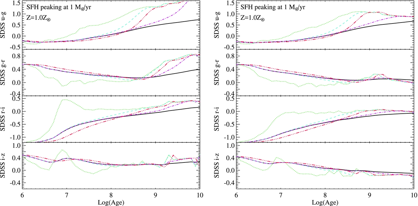
The presence of binary evolution models in a population modifies this behaviour. We can see the source of this difference in Figure 23 by comparing the single star to binary star populations. In the latter, blue stragglers and stars that have lost their hydrogen envelope to become hot helium stars appear at ages later than 10 Myrs that are not possible from a single star population. These prolong the period over which nebular emission is significant, smoothing out some of the variation in the single star models with time. Again, populations with nebular emission show redder colours at young population ages than those without, except where nebular emission lines strongly contaminate a photometric band. However, binary populations never reach the reddest colours observed in the single star models.
6.4. The local star-forming galaxy population
To provide an observational validation and test of our bpass spectral synthesis, we consider the Sloan Digital Sky Survey Data Release 7 (SDSS DR7, Abazajian et al. Reference Abazajian2009) emission line galaxy sample first explored by Brinchmann et al. (Reference Brinchmann, Charlot, White, Tremonti, Kauffmann, Heckman and Brinkmann2004) and Brinchmann et al. (Reference Brinchmann, Pettini and Charlot2008), and which has been classified by the JHU–MPA collaboration using a combination of SED fitting and strong emission line calibrations for age and metallicity. We select galaxies automatically classified as star forming rather than powered by emission from active galactic nuclei. While the caveats regarding nebular emission uncertainties discussed above apply equally to the strong line metallicity and type classifications, this sample nonetheless provides a useful point of comparison for our models.
In Figure 32, we illustrate the colours of our single-age starburst stellar models, overplotted on this SDSS galaxy data, as a function of stellar population age and metallicity. Given that in this case, no correction has been made for dust or nebular emission, the broad agreement, in terms of range of colours probed by star-forming galaxies and their trends, is good. The models sweep out much of the colour–colour space occupied by the galaxy population during their lifetime. There is evidence, however, that the simple single-age stellar models are not sufficient. The gradient of the galaxy colour–colour relation in the u − g − r plane is steeper than that of the models, while there appears to be an offset of approximately 0.2 mag in r − i, the effects of which become more apparent with increasing metallicity. There are likely several components adding to an explanation for these offsets: the role of nebular emission in modifying the continuum flux, the role of dust extinction in individual galaxies and the role of complex star-formation histories, as well as the over-representation of AGB stars in our single star models at late times. With increasing present-day metallicity, the number of permutations of these factors rises. The well-established mass–metallicity relation in the local Universe (Tremonti et al. Reference Tremonti2004) means that such galaxies are typically larger, older, and thus have been through more interactions, starbursts, and stages of galactic evolution than low-metallicity galaxies.
The photometric colours of star-forming galaxies in the SDSS survey (shown as a density map in greyscale), overplotted with the colour evolution of our models with age, assuming no effect from dust or nebular emission, and plotted as a function of metallicity. Single star tracks are plotted in red, while binary tracks are shown in blue. Tracks are plotted at ages from 1 Myr (bluest colours, i.e. lowest numerical values in u − g on each track) to 1 Gyr with 1 dex increments in age marked by crosses on the tracks.

Exploring the full parameter space of complex galaxy models is beyond the scope of this paper; the number of free parameters grows rapidly with the complexity of the model and quickly exceeds the number of constraints unless a full spectral and emission line analysis of each comparison source is undertaken. Nevertheless, to provide a slightly more realistic galaxy model for comparison with observed galaxy populations, we consider a toy stellar population that incorporates a subset of the effects discussed above. In this model, we consider an underlying old stellar population which formed its stars in a short lived exponentially decaying starburst between 3 and 1 Gyr before the present. On top of this, we impose a young starburst contributing either 1 or 50% of the stellar mass of the galaxy, with an exponentially decaying star-formation rate and a decay constant, τ = 100 Myr. Both bursts are at the current gas phase metallicity, although varying this by one bin has little effect on the galaxy colours except at the lowest metallicities. Stars are assumed to be embedded in dense nebular gas (at the same metallicity) for the first 15 Myr, and thereafter not to be modified by gas absorption or emission. We refer to this as our ‘late burst’ model. We take a minimal approach to modelling dust extinction, correcting each observed data point for internal extinction as estimated by the JHU–MPA database, and then allowing the models to vary slightly according to an additional internal dust absorption component using the Calzetti et al. (Reference Calzetti, Armus, Bohlin, Kinney, Koornneef and Storchi-Bergmann2000) dust law and an E(B − V) = 0.0, 0.05, or 0.10, before comparison with the data.
As Figure 33 demonstrates, this more complex star-formation history improves the agreement between model colours and observed data for our binary models, but worsens it for our single star models. Most of the variation in colour of the SDSS population is accounted for by fairly minor differences in dust extinction, or perhaps in appropriate extinction law, with elapsed time since the late starburst producing a spread of colours away from the dust reddening vector. Notably, when modelling this complex star-formation history, our single star models perform significantly worse, and are unable to reproduce the observed colours at most metallicities. Relatively simple star-formation histories are favoured by the single star models, but these do show the very red colours associated with over-represented AGB stars in our single star models at late times.
The photometric colours of star-forming galaxies in the SDSS survey, overplotted with the colour evolution of our complex ‘late burst’ star-formation model with age and dust extinction. Models shown incorporate an old underlying stellar population, with either 1 (solid line) or 50% of mass (dashed line) contributed by a new starburst ranging from 1 to 30 Myr in age (age along tracks). cloudy radiative transfer is used to model the nebular emission in populations up to 15 Myr in age, but this is neglected in older populations. An initial correction for internal extinction as calculated by the JHU–MPA collaboration is applied to the SDSS photometric data. Additional extinctions of E(B − V) = 0.0, 0.05, or 0.1 are applied to the models using the Calzetti dust extinction law and are shown as different tracks with the more extincted tracks moving redwards. Our single star models are shown in red and often lie off the plots, binary models are shown in blue.

6.5. Star-formation rate indicators (SFRIs)
The presence of massive stars in a population leads to distinctive emission characteristics which scale with the size of the recent star-formation event, and which are therefore used as star-formation rate indicators for unresolved stellar populations. Amongst those widely used in both the local and distant Universe are the rest-frame far-ultraviolet continuum luminosity and the luminosity of the Hα recombination line (see Kennicutt & Evans Reference Kennicutt and Evans2012, for a recent review).
Conventionally, star-formation rates are calibrated by comparing observational data to the predicted emission strength from stellar population synthesis models forming stars at a constant rate, with adjustments applied for metallicity, dust extinction, and to ensure that different star-formation rate indicators produce a consistent star-formation rate estimate for a given stellar population. Inevitably, calibration efforts focus on the well-established ongoing star-formation episodes in relatively local galaxies, and at near-Solar metallicities, with extrapolations to other environments based on a combination of empirical data and analytic projections drawn from stellar population synthesis and nebular gas modelling (e.g. Kewley, Geller, & Jansen Reference Kewley, Geller and Jansen2004).
In Figure 34, we illustrate the variation in the luminosity per stellar mass of star formation within bpass models with stellar population age, metallicity, and the presence or absence of binaries, using our standard model for nebular gas conditions as discussed in Section 6.3. We also compare these to a pair of widely used SFRI calibrations for the same observational signatures (Kennicutt & Evans Reference Kennicutt and Evans2012; Murphy et al. Reference Murphy2011). In the case of both the 1 500 Å rest-frame continuum and the Hα line, our calibrations are in good agreement with previous estimates at Solar metallicity. In the case of Hα line luminosity, the factor of 1.45 between the Kennicutt and Evans calibration and that from bpass is entirely accounted for by the adopted IMF. As discussed in Stanway et al. (Reference Stanway, Eldridge and Becker2016), the choice of 300 M⊙ for an upper mass limit leads to a 45% increase in the ionising photon production (and hence Hydrogen recombination line flux) relative to an IMF with a maximum of stellar mass of 100 M⊙, while the effect of the most massive stars on the rest-frame ultraviolet continuum (which is built up from a broader range of stellar masses) is less dramatic.
The evolution of key star-formation rate indicators for young stellar populations. We show values for three metallicities (corresponding to 0.05, 0.5, and 1 Z⊙) and for populations incorporating binaries (colour) and without binaries (greyscale with matching linestyle). The solid horizontal line in each case indicates the calibrations recommended by Kennicutt & Evans (Reference Kennicutt and Evans2012).
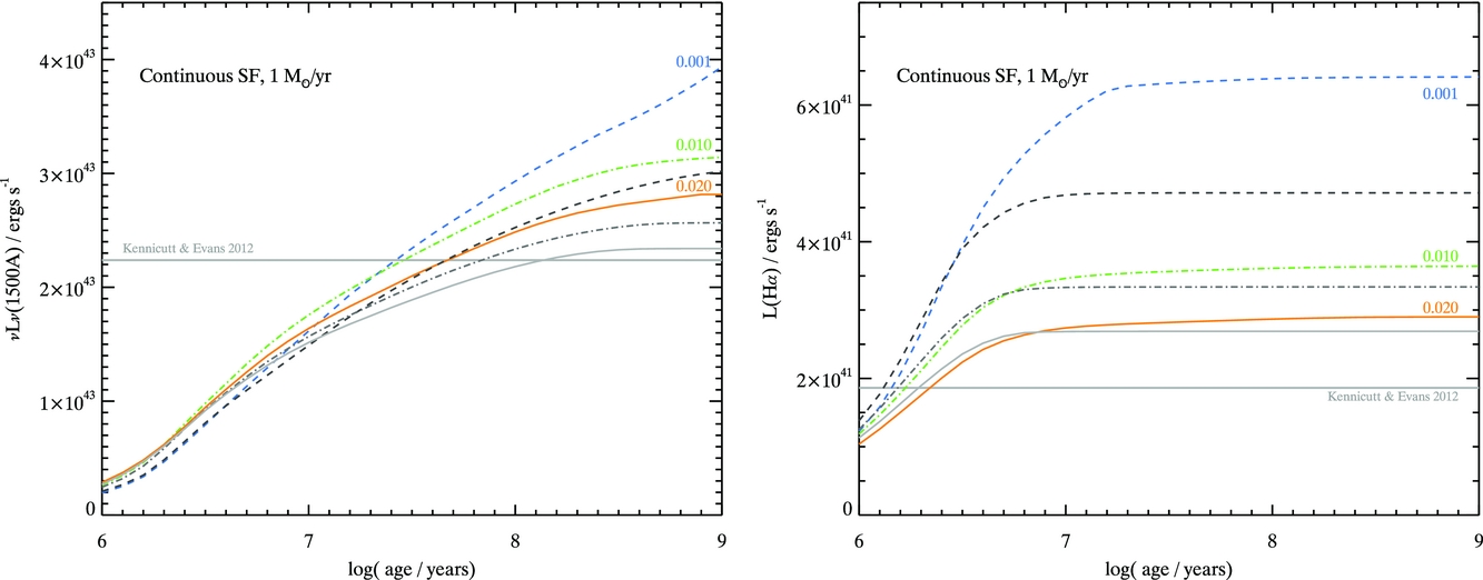
When deviating from near-Solar metallicities, bpass typically predicts a higher luminosity for a given star-formation rate (or, alternately, fewer stars being formed for a given observed flux) than previous calibrations. This is particularly true when binaries are incorporated into the population synthesis. Quantitative results as a function of metallicity and binary/single star model are given in Table 4, where these values are quoted at an age of 108.5 yrs after the onset of constant star formation. Values in this table can be utilised as star-formation rate conversions using the prescription:
 $$\begin{equation}
\log (\dot{\mathrm{M}} / \mathrm{M}_\odot \,\mathrm{yr}^{-1}) = \log (L / \mathrm{erg\,s}^{-1}) - C(Z),
\end{equation}$$
$$\begin{equation}
\log (\dot{\mathrm{M}} / \mathrm{M}_\odot \,\mathrm{yr}^{-1}) = \log (L / \mathrm{erg\,s}^{-1}) - C(Z),
\end{equation}$$
where L is the relevant observed luminosity and C(Z) is the metallicity-dependent value given in the table.
The predicted luminosity corresponding to a constant star-formation rate of 1 M⊙ yr−1, i.e. values of C(Z).
a, b log10(luminosity/ergs s−1) at log(age/yrs) = 8.5.
c For an IMF truncated at a stellar mass of 100 M⊙.
d The recommended calibration of Kennicutt & Evans (Reference Kennicutt and Evans2012).
It should be noted that Figure 34 also demonstrates the key importance of understanding star-formation timescale when attempting to apply a star-formation calibration to an unresolved star-forming system, particularly in the distant Universe where stellar populations are typically younger. Single star populations forming stars at a continuous rate reach a stable calibration for Hα by about 5 Myr after the onset of star formation, and in the UV after about 100 Myr. By contrast, binary populations take longer to establish a constant star-formation rate to luminosity relation and in some cases, as for the rest-frame ultraviolet continuum at the lowest metallicities, it is not clear that this ever occurs. This time-dependent conversion factor needs to be considered when assigning star-formation rates to galaxies or unresolved stellar clusters at stellar ages of less than a few hundred Myr (see also Greis et al. Reference Greis, Stanway, Levan, Davies and Eldridge2017).
6.6. The distant galaxy population
A number of recent publications have suggested that star-forming galaxies in the distant (z > 2) Universe may show signs of a harder typical ultraviolet radiation field than is common in the local Universe (e.g. Steidel et al. Reference Steidel, Strom, Pettini, Rudie, Reddy and Trainor2016; Stark et al. Reference Stark2015; Stanway et al. Reference Stanway, Eldridge, Greis, Davies, Wilkins and Bremer2014). These galaxies are selected primarily on the presence of a Lyman break in their rest-frame ultraviolet continuum (Lyman break galaxies or LBGs, Steidel & Hamilton Reference Steidel and Hamilton1992) or strong Lyman alpha emission (LAEs, e.g. Cowie & Hu Reference Cowie and Hu1998). The galaxies are typically younger and have simpler stellar populations than in local star forming populations, and they are also likely at significantly sub-Solar (<0.5 Z⊙) metallicities. As Figure 6 made clear, the role of binaries on extreme ultraviolet emission is a strong function of metallicity.
This is an active and rapidly developing area of research that will likely be revolutionised by the imminent launch of the James Webb Space Telescope (JWST). The NIRSPEC instrument will enable deep spectroscopy of hundreds (if not thousands) of star-forming galaxies at 3 < z < 8, from the rest-frame ultraviolet through to the rest-optical (see e.g. Giardino et al. Reference Giardino, Skillen, Barcells and Trager2016). As discussed in Stanway (Reference Stanway2016), the use of binary evolution models such as bpass may well be necessary to model such galaxies and a number of papers have already been published exploring this area, notably Steidel et al. (Reference Steidel, Strom, Pettini, Rudie, Reddy and Trainor2016) on applications to galaxies at Cosmic Noon (z ~ 2 − 3), Stanway et al. (Reference Stanway, Eldridge and Becker2016) and Ma et al. (Reference Ma, Hopkins, Kasen, Quataert, Faucher-Giguère, Kereš, Murray and Strom2016) on implications for reionisation and Wilkins et al. (Reference Wilkins, Feng, Di-Matteo, Croft, Stanway, Bouwens and Thomas2016) for application to semi-analytic galaxy evolution modelling. Here we summarise some key observational tests and applications of bpass in this regime and the key differences between version 2.1 and our earlier v2.0 models.
6.6.1. Ionising photon production efficiency
A key parameter for constraining the reionisation history of the Universe, and one of the most significant to change behaviour between bpass v2.0 and v2.1, is the ionising photon production efficiency $\xi _{\mathrm{ion}} = \dot{N}_\mathrm{ion}/f_\mathrm{esc}\,L_\mathrm{UV}$
, i.e. the ratio between the ionising photon production rate and the rest-frame ultraviolet continuum luminosity for a given fraction of such photons which escape their host galaxy. While the luminosity can be directly observed in the distant Universe, the ionising photon production rate must be inferred from either models or indirect observations of the strong nebular emission lines generated from the galaxy in question, assuming that a fraction (1 − f
esc) of the ionising continuum is absorbed by the interstellar medium.
$\xi _{\mathrm{ion}} = \dot{N}_\mathrm{ion}/f_\mathrm{esc}\,L_\mathrm{UV}$
, i.e. the ratio between the ionising photon production rate and the rest-frame ultraviolet continuum luminosity for a given fraction of such photons which escape their host galaxy. While the luminosity can be directly observed in the distant Universe, the ionising photon production rate must be inferred from either models or indirect observations of the strong nebular emission lines generated from the galaxy in question, assuming that a fraction (1 − f
esc) of the ionising continuum is absorbed by the interstellar medium.
For simplicity, an escape fraction f esc = 0 is often assumed, yielding ξ0,ion, but in practice the paradigm that the intergalactic medium is ionised by early star formation, and that ionisation state is maintained over cosmic time, requires a much higher escape fraction. Observations aimed at constraining that escape fraction compare measured luminosities at wavelengths shortwards of the ionisation edge of hydrogen at λ(rest) = 912 Å with models of what flux the stellar population is expected to produce, given the observed 1 500 Å luminosity. ξ0,ion is thus a crucial parameter both for estimation of escape fraction and for interpretation of the effects of star-forming galaxies on the reionisation epoch.
Between v2.0 and v2.1, we have made two important changes to the models that affect this parameter: we have extended our models to still lower metallicities, and we have improved the stellar atmosphere models in use for the highest gravity O stars (see Section 2.3.2). These models are particularly important at low metallicities (where mass loss is lowest and stars can thus remain more massive), and in the rotationally mixed stars which dominate the ionising photon production.
In Figure 35, we present a direct comparison between our previous estimates of ionising photon production rate, ultraviolet luminosity, and thus ξ0,ion and new estimates from v2.1 for the case of continuous star formation observed at 100 Myr after the onset of the star-formation epoch. There are three clear differences in behaviour between our improved v2.1 models and the older v2.0 models. First, v2.1 does not show the dramatic increase in ionising photon production rate at metallicities below Z = 0.004, which was associated with the onset of quasi-homogenous chemical evolution—while this still leads to increased photon production, it is moderated by the new atmosphere models. Second, the v2.1 models are more luminous in the rest-frame ultraviolet than the v2.0 models and the difference between single and binary models has narrowed due to a more rapid build up of continuum flux than in our previous models. Third, as a result of these behaviours, the metallicity evolution of the ionising photon production efficiency has become less clear cut. In v2.0, the binary population always exceeded the single star population in ξ0,ion at a given metallicity. In v2.1, we see lower photon production efficiencies in the binary population than in single stars at metallicities above ~0.3 Z⊙ in our standard IMF, and near-equal efficiencies in IMFs excluding the most massive stars. This behaviour reverses at lower metallicities, where the binary population continues to dominate.
A comparison between the ionisation characteristics of bpass v2.0 and v2.1 models for a population which has been continuously forming stars at a rate of 1 M⊙ yr−1 over a 100 Myr period, shown as a function of metallicity. In the top panel, we show the small effect of our improved atmosphere models on the ionising photon production rate. By contrast, the centre panel shows a strong change in rest-ultraviolet luminosity between v2.0 and v2.1. As a result, the lower panel shows a change in the behaviour in ξ0,ion. Single star models are shown with dashed lines, while binary models are shown with solid lines. Our standard IMF is shown (labelled imf300), with an identical IMF with M max = 100 M⊙ also given for comparison.
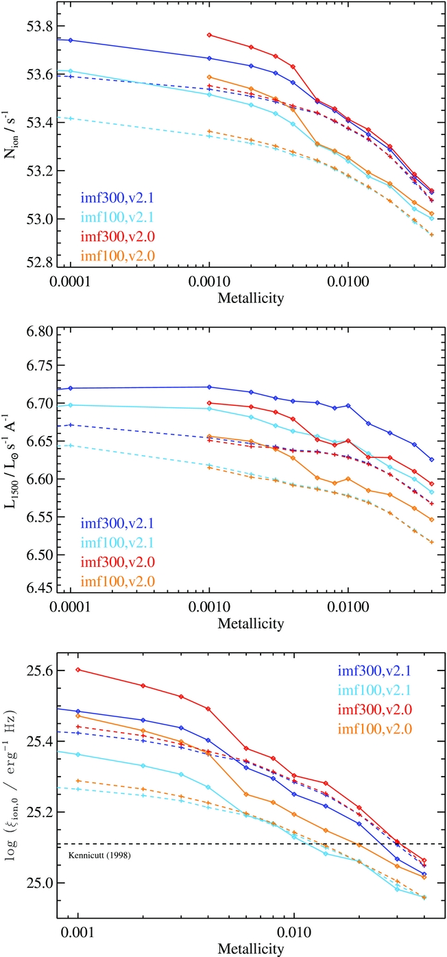
This behaviour is entirely driven by the behaviour of the youngest stars in a given population. As Figure 36 demonstrates, the ionising photon production output of a single-aged, instantaneous-starburst binary population exceeds that of the single star population at all metallicities for ages >3 Myr but the stars below this age produce photons with a far higher efficiency. In the low metallicity populations, the longer ionising photon production lifetime of the binary stars leads to the binary population overtaking the single stars at late ages for any ongoing or evolving starburst, while at near-Solar metallicity the rapid mass loss due to stellar winds dominates over binary effects.
The time evolution of ionising photon production efficiency as a function of star-formation history shown for metallicities of ~Z⊙ and 0.1 Z⊙. Single star models are shown in greyscale, with dashed lines, while binary models are shown in colour with solid lines. The star-formation histories shown are those defined in Figure 29.
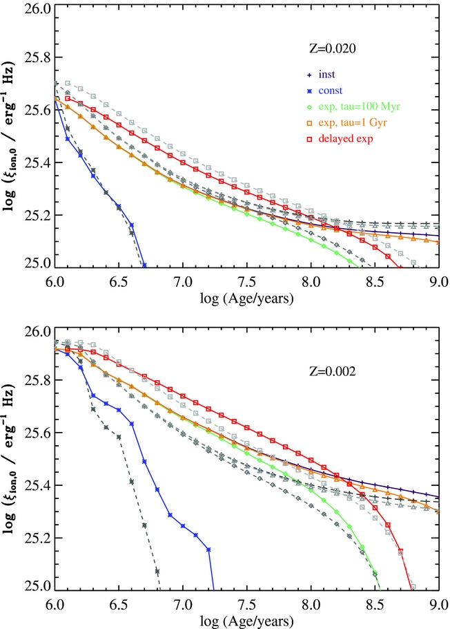
The decrease in overall ionising photon efficiency in bpass v2.1 relative to v2.0 reflects an improvement in stellar atmosphere modelling, but also emphasises the significant uncertainties in the stellar models, particularly in the low metallicity regime, and thus the difficulty of interpreting distant galaxies. We note that an improved treatment of rotation (see Section 7.2) could reverse the shift seen in this version.
In Figure 37, we compare our current predictions for ionising photon efficiency with observational constraints. These are drawn from the literature and based on a standard analytic conversion from Hα emission line flux to ionising photon production rate (which itself is somewhat model dependent). Distant galaxies are shown as shaded regions indicating the mean and standard deviation of the (often small) measured sample in ξ0,ion. The metallicity is poorly constrained in these observations and samples are shown offset to indicate a plausible range in metallicity mass fraction. We also show data for a sample of extreme local starburst galaxies identified as analoguous to the z ~ 5 galaxy population for which metallicity information can be inferred from the optical spectra and allows the data to be binned (Greis et al. Reference Greis, Stanway, Davies and Levan2016). In previous versions of this comparison, we have considered a model population continuously forming stars at 1 M⊙ yr−1 over 100 Myr; now we compare with models at 10 Myr after the onset of star formation although, as Figure 29 demonstrated, an alternative approach would be to assume a more bursty and less constant star formation history.
The ionising photon production efficiency as a function of metallicity and star-formation history for an ongoing star-formation event which has formed stars continuously over the previous 10 Myr. Grey regions indicate measured values of ξ0,ion in the distant Universe together with their uncertainties. These samples are unconstrained in metallicity and are shown offset to indicate plausible metallicity ranges given BPASS population synthesis models. Data points show results for a sample of local extreme star-forming galaxies (Lyman Break analogues) from Greis et al. (Reference Greis, Stanway, Davies and Levan2016), binned by optical emission line metallicity. Star-formation histories are colour-coded as in Figure 36.
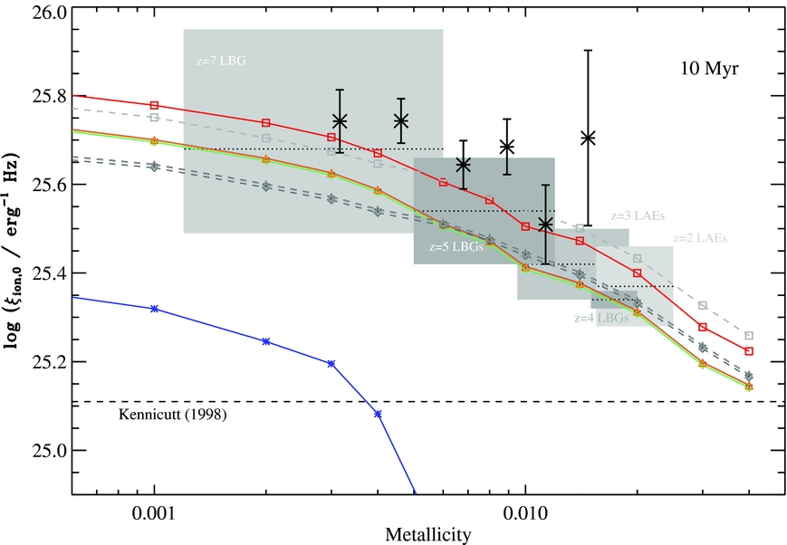
As can be seen, a single age starburst would struggle to reproduce the high ξ0,ion values inferred from both distant and local extreme starburst observations, unless captured in the very first few million years. By contrast, an ongoing or rising starburst history provides a reasonable match to the observed data at ages of order ~10 Myr.
6.6.2. Optical recombination line ratios
In Stanway et al. (Reference Stanway, Eldridge, Greis, Davies, Wilkins and Bremer2014), we demonstrated that, subject to the usual uncertainties in nebular gas conditions, our v1.1 single age starburst models were capable of reproducing the optical strong line ratios seen in the z ~ 2 − 3 galaxy population. In Figure 38, we update this comparison incorporating our newer v2.1 models. For consistency, we use the same nebular emission model as in the above work, with a fixed electron density (100 cm−3) and cloud geometry (spherical, 10 pc inner radius), and allow stellar population age to vary along tracks. We confirm our earlier finding that young stellar populations incorporating binary evolution pathways can reproduce both the strong line ratios and the Hβ equivalent widths seen in the distant population, while single star models struggle to do so.
The evolution in Balmer emission line strength and [O iii]/Hβ line ratio with stellar population age. Age increases along the tracks from high equivalent width to low. Tracks for binary models are shown in colour and those for single star models in greyscale, with different line styles. Overplotted are the data for star-forming galaxies at z = 2 − 3 reported by Holden et al. (Reference Holden2016, triangles) and Schenker et al. (Reference Schenker, Ellis, Konidaris and Stark2013, squares). Greyscale indicates the measured properties of the local SDSS star-forming galaxy population.
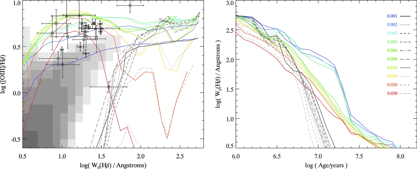
We also show the measured properties of the SDSS star-forming galaxy population, as defined above. Interestingly, these show an offset from both the binary and single star model populations, lying between the two but more consistent with the binary tracks. We note that these have not been corrected for internal dust extinction (which may affect lines more strongly than continuum in some extinction models, and so would push the data towards the single star tracks in equivalent width) but are corrected for fibre losses. We consider only a simple star-formation history in this case, since the line emission spectrum is heavily dominated by the youngest starburst. A more complex star-formation history will tend to slightly reduce the model Hβ equivalent width, again pushing the data towards the single star models. However, as Figure 38 also demonstrates, the evolution of the single star models in line equivalent width is extremely rapid, and so the SDSS population would have to be caught in a very narrow time window some 10 Myr after the onset of star formation. By contrast, the binary models provide high Hβ equivalent width over a more extended time period increasing the probability of populating the parameter space occupied by the SDSS sources. If binary evolution models are preferred, there are two likely explanations for the offset of the SDSS galaxies from our models. The first may be use of an inappropriate gas density or cloud geometry for the local population—adjusting these will tend to reduce the model [O iii]/Hβ ratio at a given Hβ equivalent width, bringing the binary models better in line with the data (see Stanway et al. Reference Stanway, Eldridge, Greis, Davies, Wilkins and Bremer2014). Alternately, the binary distribution parameters assumed (see Table 1), which appear to reproduce those in the distant Universe and simple massive stellar populations, may overestimate the interacting binary fraction in high metallicity galaxies in the local Universe with more complex star-formation histories and old underlying stellar populations. The result of assuming a lower binary fraction in low mass stars would be to move the binary models towards the local galaxy data, as further discussed in Section 7.10.
In Figure 39, we show an alternate ionisation diagnostic—the Baldwin, Phillips, & Terlevich (Reference Baldwin, Phillips and Terlevich1981, BPT) diagram widely used to distinguish emission powered by star-forming regions from that powered by accretion onto an AGN. We show the locus occupied both by local star-forming galaxies (greyscale) and the distant galaxy population reported by Steidel et al. (Reference Steidel, Strom, Pettini, Rudie, Reddy and Trainor2016, data points). Overlaid are evolutionary tracks for a co-eval simple stellar population with age, at a range of metallicities, assuming the same simple nebular model as above. At ages of ~10 Myr, the tracks cross the Kauffmann et al. (Reference Kauffmann2003) boundary for separating local star-forming galaxies, and, as before, more complex star-formation histories are required to overlay the SDSS galaxy population, which typically lies somewhere between the ratios expected for a single age starburst and constant, ongoing star formation. A full exploration of the BPT parameter space occupied by bpass models with different assumed nebular gas conditions will be presented in Xiao et al. (Reference Xiao2017).
The evolution of strong optical emission line ratios with stellar population age. Age increases along the tracks from 1 Myr to 30 Myr for instantaneous burst models. Small circles are data for star-forming galaxies at z = 2 − 3 reported by (Steidel et al. Reference Steidel, Strom, Pettini, Rudie, Reddy and Trainor2016). An indicative typical error bar for the data is shown at the bottom right. Greyscale indicates the measured properties of the local SDSS star-forming galaxy population. The solid grey line shows the Kauffmann et al. (Reference Kauffmann2003) condition for distinguishing regions ionised by AGN from star forming galaxies. Triangles indicate the line ratios expected for a binary stellar population with constant star formation over the last 100 Myr.

An additional validation test for our models, and an important demonstration of the ambiguity that arises from nebular gas parameters, is their ability to reproduce the line ratios seen in GRB host galaxies. The presence of a GRB requires these galaxies to have formed massive stars recently, and thus (as with the WR-galaxies discussed above) their nebular emission tend to be dominated by a young stellar population. We consider here the TOUGH sample, observed spectroscopically by Krühler et al. (Reference Krühler2015) with X-SHOOTER on the ESO VLT, for which metallicity and extinction estimates are available. In Figure 40, we consider a third diagnostic line ratio, [OII] λ3726,3729 Å/[OIII]λ5007 Å. The evolution of this line ratio is not entirely smooth in either stellar population age or nebular electron density, with both playing an important role in exciting these forbidden lines. Nonetheless, considering a range of plausible ages (1 to 100 Myr) and electron densities (0.1 to 1000 cm−3) makes clear the locus of permitted line ratios relative to [OIII]/Hβ and their good agreement with the observed properties of GRB hosts (upper panel). Solid lines indicate a polynomial fit to the variation with age at each metallicity and demonstrates the relative insensitivity of this parameter space to metallicity in the range Z ~ 0.5–0.7 Z⊙, but also the significant scatter around the mean locus given a range of assumptions regarding age and nebular gas conditions. This point is perhaps still clearer in Figure 40 (right-hand panel), which shows the evolution in [OII]/[OIII] as a function of metallicity at three stellar population ages and three gas densities. There is significant degeneracy between different plausible models. If interpreted at fixed age and electron densities, the distribution of [OII]/[OIII] line ratios seen in the GRB hosts of Krühler et al. (Reference Krühler2015) is consistent with a metallicity sequence. However, a variation in stellar population age, or electron density, or both, at fixed metallicity could also provide a good fit to the observations. Given that the metallicities shown for the data points were themselves derived from the optical recombination line spectrum, and thus ultimately derive from a photoionisation model and stellar population fit to a calibration data set, the correct interpretation is unclear, and likely involves some evolution in all three parameters.
The emission line properties of GRB host galaxies compared to BPASS v2.1 models. Both panels consider the [OII]/[OIII] excitation diagnostic. In the left-hand panel small coloured points indicate the predicted line fluxes for models with ages from 1 Myr to 100 Myr, and at electron densities ranging from 0.1 to 1000 cm−3. Solid lines are a polynomial fit to all models with n e = 100 cm−3 as a function of metallicity and indicate the general trend in the permitted parameter space. The right-hand panel shows the [OII]/[OIII] ratio explicitly as a function of metallicity at three stellar population ages, and three electron densities, showing the ambiguity between an older population and a sparser ISM at any given metallicity. GRB host galaxy data are taken from Krühler et al. (Reference Krühler2015) and are shown in black for hosts at z > 1 and in grey for hosts at z < 1, metallicities for data points are those derived from optical strong line ratios by Krühler et al. (Reference Krühler2015). Only objects with measurements in all relevant quantities, and an estimated E(B − V) < 0.2 are shown. Line ratios have been corrected for internal extinction using the Calzetti dust law.
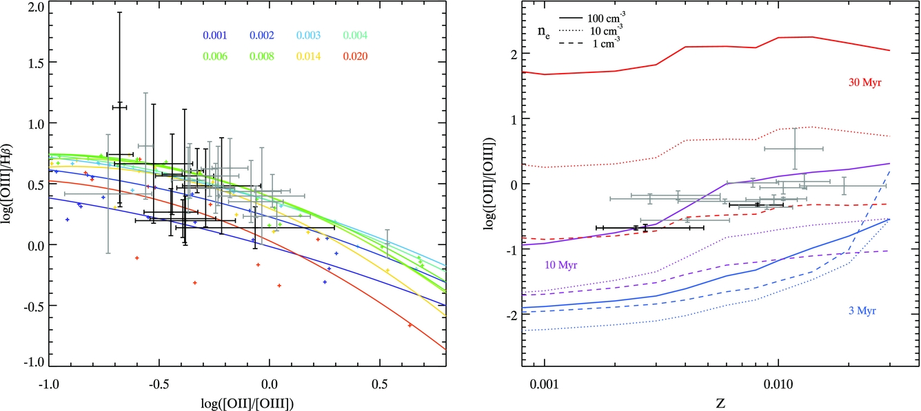
6.6.3. Ultraviolet spectral features
Ultraviolet emission lines, redshifted into the observed frame optical and near-infrared are crucial evidence for the stellar populations and properties of distant galaxies. A recent study by Bowler et al. (Reference Bowler, McLure, Dunlop, McLeod, Stanway, Eldridge and Jarvis2016) has already made use of beta versions of our lowest metallicity v2.1 models to explore the interpretation of the anomalous source CR7 (Sobral et al. Reference Sobral, Matthee, Darvish, Schaerer, Mobasher, Röttgering, Santos and Hemmati2015) which has been proposed as either a Population III starburst or, potentially, a direct collapse black hole. While none of the model sets explored in that work provide an unambiguous interpretation for CR7, bpass low metallicity, young starburst models are broadly consistent with the colours of the source in question (particularly if some degree of enhancement in α-elements is assumed) suggesting a stellar origin for the light. The extreme properties of CR7 (specifically its He ii line strength) have recently been challenged (Shibuya et al. Reference Shibuya2017). Nonetheless, this source and the similar high redshift emission line sources now being identified provide one of the very few constraints on our models at the lowest metallicities. Crucially, they are representative of a regime that may soon be more widely explored by JWST.
As is the case for optical lines, interpretation of the ultraviolet spectrum of a complex stellar population requires an assumption regarding the nebular gas conditions, which are largely unconstrained by observations. Steidel et al. (Reference Steidel, Strom, Pettini, Rudie, Reddy and Trainor2016) have suggested that the spectra of galaxies at z ~ 2 − 3 are best fit by combining very low metallicity stellar spectra (the observed properties of which are most strongly influenced by the iron abundance) with somewhat higher metallicity nebular gas (the properties of which are dominated by oxygen abundance). Again, this may be indicative of strong α-element enhancement, as would be expected in the young stellar populations at this redshift.
The difficulty in evaluating nebular effects is particularly true of resonantly scattered lines such as the Lyman-α feature, the ratio of which to the Balmer series is shown in Figure 41 for a continuously star-forming population, assuming our usual gas geometry and local electron densities ranging from 1 to 104 cm−3. In Figure 42, we simply assume n e = 102 cm−3 and Z(nebular) = Z(stellar), in order to demonstrate emission line strengths as a function of age and metallicity for our standard cloudy models, normalised relative to the Lyman-α line strength in the same galaxy. Perhaps, the most striking effect of decreasing metallicity is the increase in strength of rest-frame ultraviolet emission lines that are seldom seen in normal stellar populations in the local Universe, and which are usually associated with emission from AGN when observed. These lines are not significantly excited in nebular gas irradiated by our equivalent single star models.
The ratio of intrinsic Lyman-α emission to optical Balmer line ratio assuming a range of metallicities and gas parameters. While the Balmer line ratio is only weakly sensitive to the environment, Lyman-α is strongly affected by the metallicity and physical conditions of the nebular gas. Electron densities increase from 1 cm−3 to 104 cm−3 along coloured (fixed metallicity) lines and are marked at 1 dex intervals. We assume constant star formation, observed at age 108 years.
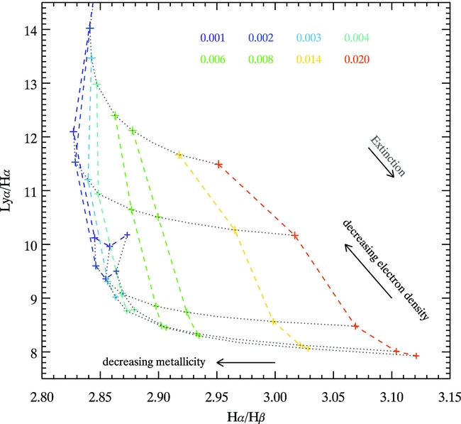
The evolution in rest-frame ultraviolet emission line flux ratios for a single-aged simple stellar population at four representative metallicities. Line strengths shown are normalised relative to the Hydrogen Lyman-α λ1216 Å feature, and are He ii λ1640 Å, C iii] λ1909Å, and O iii] λ1665 Å. For doublets, the total flux is given.
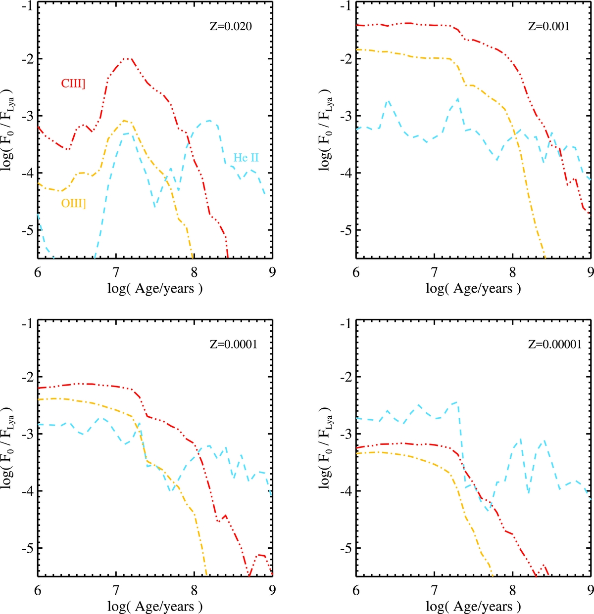
At the lowest metallicity in our models (Z = 1 × 10−5 = 0.05% Z⊙), He ii λ1640 Å is the strongest emission line in the rest-UV longwards of the Lyman-α line. At the low to moderate metallicities, more typical of the distant Universe (0.5 to 10% Z⊙), the semi-forbidden doublets of C iii] λ1909 Å and O iii] λ1665 Å increasingly exceed the helium line in line flux. All three species decline in strength towards Solar metallicity due to the decline in ionising photon strength emitted by stellar populations.
The [C iii] λ1907Å, Ciii] λ1909 Å doublet has attracted particular attention of late as the result of its detection in a handful of very distant (z > 6) star-forming galaxies (Stark et al. Reference Stark2015, Reference Stark2017), and its position in the rest-frame ultraviolet, which means it is observable in the optical in the distant Universe. This line may arise from the atmospheres and winds of massive stars (in which case it will typically be broad) and from ionised nebular gas in H ii regions (in which it is typically narrow). Both of these are seen locally in the environs of WR stars and planetary nebulae (e.g. Guerrero & De Marco Reference Guerrero and De Marco2013). Observed lines in distant sources tend to be narrow, suggesting a nebular origin, but the constraints on its velocity width are relatively poor in most cases. In Figure 43, we show the predicted total equivalent width of this doublet as a function of stellar population age and metallicity for a population continuously forming stars at 1 M⊙ yr−1, after passing through nebular gas. These are compared to the distribution of measured rest-frame equivalent widths in this doublet arising from star-forming galaxies at z = 0–8 (Stark et al. Reference Stark2014; Rigby et al. Reference Rigby, Bayliss, Gladders, Sharon, Wuyts, Dahle, Johnson and Peña-Guerrero2015; Vanzella et al. Reference Vanzella2016; Patrício et al. Reference Patrício2016; Du et al. Reference Du, Shapley, Martin and Coil2017, Maseda et al. Reference Maseda2017). We also indicate the rest-frame equivalent widths measured for four stacks of z ~ 3 LBGs, sorted into quartiles by Lyman-α equivalent width and each containing ~200 galaxies, by Shapley et al. (Reference Shapley, Steidel, Pettini and Adelberger2003). Unsurprisingly, the bulk of the observed measurements are consistent with the very low equivalent widths we expect for mature stellar populations at moderate metallicities. It is notable however that, at both z < 3 and z > 3, there exists a tail of sources extending to $W_{\rm {0,C {\rm iii]}}}>10$
Å. Comparison with our standard cloudy models suggest that these are most naturally explained by stellar populations with significantly sub-Solar metallicities, Z < 0.2 Z⊙, or very young dominant stellar populations (<10 Myr). In the most extreme observed cases, both of these conditions may be necessary. At the very lowest metallicities in the bpass model set (Z < 0.05% Z⊙), the hard stellar ionising spectrum excites very little C iii] emission simply because of the scarcity of carbon atoms in the nebular gas. As observations approach this regime in the very distant Universe, it is worth noting that, in the presence of a carbon-enriched ISM, the irradiating spectrum will likely excite strong line emission and that such enrichment may result from massive stellar explosions very rapidly after the onset of star formation. As discussed before, there is scope for further populating this parameter space by varying electron density, local ionisation parameter, and potentially the α-element enhancement of the nebular gas. However, the C iii] doublet is of particular interest since its line ratio is itself sensitive to electron density and thus potentially allows some such degeneracies to be broken. As samples of deep rest-frame ultraviolet spectra grow, it will likely be possible to break many such degeneracies with observations of both the doublet line ratio and further emission lines in future.
$W_{\rm {0,C {\rm iii]}}}>10$
Å. Comparison with our standard cloudy models suggest that these are most naturally explained by stellar populations with significantly sub-Solar metallicities, Z < 0.2 Z⊙, or very young dominant stellar populations (<10 Myr). In the most extreme observed cases, both of these conditions may be necessary. At the very lowest metallicities in the bpass model set (Z < 0.05% Z⊙), the hard stellar ionising spectrum excites very little C iii] emission simply because of the scarcity of carbon atoms in the nebular gas. As observations approach this regime in the very distant Universe, it is worth noting that, in the presence of a carbon-enriched ISM, the irradiating spectrum will likely excite strong line emission and that such enrichment may result from massive stellar explosions very rapidly after the onset of star formation. As discussed before, there is scope for further populating this parameter space by varying electron density, local ionisation parameter, and potentially the α-element enhancement of the nebular gas. However, the C iii] doublet is of particular interest since its line ratio is itself sensitive to electron density and thus potentially allows some such degeneracies to be broken. As samples of deep rest-frame ultraviolet spectra grow, it will likely be possible to break many such degeneracies with observations of both the doublet line ratio and further emission lines in future.
The rest-frame equivalent width of the (unresolved) [C iii] λ1907 Å, C iii λ1909 Å doublet, as a function of stellar population age and metallicity for a population continuously forming stars at the rate of 1 M⊙ yr−1. In the right-hand panel, we compare these predictions to the distribution of measured C iii 1909 lines in star-forming galaxies compiled from the literature (see Section 6.6.3). Measurements from sources at z > 3 are highlighted in red, while arrows indicate the measurements obtained from stacks of z ~ 3 Lyman break galaxies differing in Lyman-α line strength (Shapley et al. Reference Shapley, Steidel, Pettini and Adelberger2003).
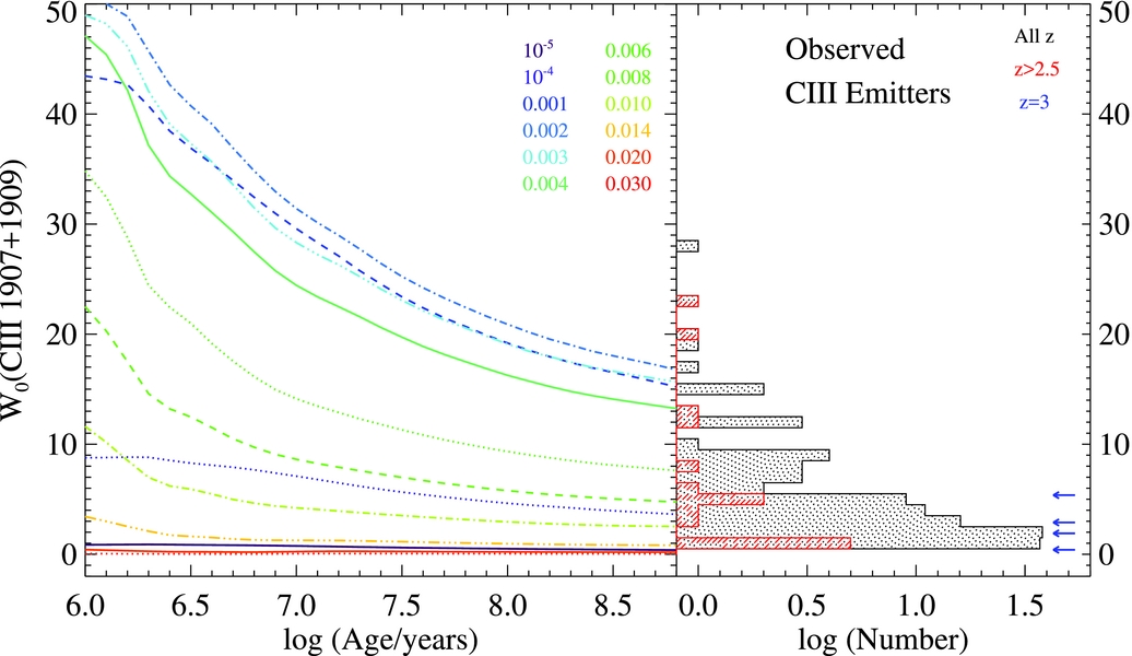
A fuller exploration of the limited observational data on nebular line emission at high redshift is deferred to later work.
7 FUTURE WORK AND UNCERTAINTIES
Any numerical model, no matter how much effort is expended in its creation, will always be subject to limitations. It is vital to make important caveats clear, as well as their impact on any predictions from that model. Here we outline these for the bpass code and highlight how we aim to resolve them in future versions of the code.
7.1. Secondary stars
A key feature of the bpass models that sets them apart from others, except the Brussels code (Vanbeveren et al. Reference Vanbeveren, De Loore and Van Rensbergen1998; Mennekens & Vanbeveren Reference Mennekens and Vanbeveren2016), is that all the interacting binary evolution models are evolved in a full detailed stellar evolution code. This is in contrast to the approximation methods employed by rapid population synthesis codes (e.g. Hurley et al. Reference Hurley, Tout and Pols2002). The rapid method allows for the uncertainties of binary evolution and their impact on predictions to be explored; this would be too computationally intensive for detailed stellar models. The use of detailed models, on the other hand, allow us to accurately follow how the stellar envelope responds to mass loss—key to determining the eventual mass and fate of the star.
This impacts on our treatment of the secondary stars. In a binary system after the first supernova, the future evolutionary pathways are varied. The system can be unbound so the secondary continues its evolution as a single star, or the binary can remain bound in a range of possible orbits. For rapid population synthesis, it is straightforward to simply calculate each possibility as they occur, but in a detailed code, this becomes more numerically intensive. Our current solution is to use single star models to represent the evolution when systems are unbound. The range of bound systems is also determined and a range of secondary models calculated in which one of the stars is a compact remnant.
However, a complication arises with how to deal with mass transfer. If the secondary star accretes material (mostly hydrogen) from the primary, we use its final accreted mass at the end of mass transfer as its effective initial mass when selecting a model to represent its subsequent evolution. If this effective initial mass is greater than 105% of the actual initial mass, then we treat the model as rejuvenated. We use the age of the primary model as an estimate of the rejuvenation age, this is a reasonable approximation for stars that end in a core-collapse supernova but as noted above an overestimate when a white dwarf is formed. Our secondary model contribution to the whole population is split into models that have not interacted but have simply increased in mass and those that have been rejuvenated, and their contribution is offset in time so that their zero-age is at the post-rejuvenation age.
The disadvantage of this approach is that we do not model the intricacies of mass accretion onto the secondary stars in detail, and thus do not accurately trace the post-accretion evolution. We simply assume these secondary stars become fully mixed, more massive, main-sequence stars. There is observational evidence that such stars can actually appear very different (e.g. Smith & Tombleson Reference Smith and Tombleson2015). The way to improve this is to calculate the accretion onto the secondary in more detail and then calculate its evolution after that accretion. We aim to do this in future but the computational demands are beyond the scope of bpass v2.1 models. The practical outcome of this is that we may underestimate the number of BSGs and related objects in our simulations.
7.2. Rotation and quasi-chemically homogeneous evolution
We currently only consider rotation in two contexts. One is to follow the transfer of angular momentum between the stars and orbit during RLOF and allow for this to instigate common-envelope evolution. The second is in our model of rejuvenation. We assume that if more than 5% of a star’s initial mass is accreted, the star rotates rapidly enough to be fully mixed. Furthermore, at low metallicites, Z ⩽ 0.004, if this occurs for stars more massive than 20 M⊙, it is assumed to be fully mixed during its entire main-sequence lifetime, experiencing QHE, and the model is replaced by a model that is fully mixed until it loses all hydrogen. In nature, it is more likely there is a continuum of behaviour that we are unable to reproduce without a more sophisticated implementation of rotation in our evolution code. Again this is a factor we will return to and improve in future. We also note that QHE may occur due to tidal forces in binary stars at the relatively high metallicity of the LMC (Shenar et al. Reference Shenar2017) as well as lower metallicities. This is not currently included in any bpass models but is potentially important for gravitational wave sources (de Mink et al. Reference de Mink, Langer, Izzard, Sana and de Koter2013; Marchant et al. Reference Marchant, Langer, Podsiadlowski, Tauris and Moriya2016).
There is some evidence that such a simple model can work, however. de Mink et al. (Reference de Mink, Langer, Izzard, Sana and de Koter2013) included a model of rotation in a rapid population synthesis code and found that mass transfer mainly leads to creating rapidly rotating stars during break up, and furthermore that the predicted rotational distribution is similar to that observed in nearby star-forming regions. Our current prescription behaves similarly. Thus, while some refinements may be required in specific contexts, we must already reproduce the broad range of behaviour. We note that the primary effect of increasing the number of rotating stars is likely to be boosting the ionising photon flux from a population.
7.3. Roche lobe overflow, common envelope evolution, and mergers
Our model of RLOF is relatively unsophisticated and we may update it in future with more realistic models (e.g. Ritter Reference Ritter1988; Kolb & Ritter Reference Kolb and Ritter1990; Sepinsky et al. Reference Sepinsky, Willems and Kalogera2007). The complexities of CEE are less uncertain than they used to be, as a result of extensive hydrodynamic simulations in recent years (e.g. Passy et al. Reference Passy2012; Ricker & Taam Reference Ricker and Taam2012; Nandez & Ivanova Reference Nandez and Ivanova2016; Ohlmann et al. Reference Ohlmann, Röpke, Pakmor and Springel2016; Staff et al. Reference Staff, De Marco, Macdonald, Galaviz, Passy, Iaconi and Low2016; Iaconi et al. Reference Iaconi, Reichardt, Staff, De Marco, Passy, Price, Wurster and Herwig2017), although this work focuses on low mass (~1–2 M⊙) giants. However, while our straight-forward binding/orbital energy prescription for CEE provides results in line with current thinking, how best to model the CEE phase within a 1D hydrostatic evolution code is still unclear (Ivanova et al. Reference Ivanova2013).
The only way to improve this model is for more CEE events to be observed and their properties used to refine models: this may include recently observed examples such as those detailed by Blagorodnova et al. (Reference Blagorodnova2017) and MacLeod et al. (Reference MacLeod, Macias, Ramirez-Ruiz, Grindlay, Batta and Montes2017). Work to unify such observations with simulations is ongoing (e.g. Galaviz et al. Reference Galaviz, De Marco, Passy, Staff and Iaconi2017). It may also be necessary in future to model post-CEE systems such as white-dwarf binaries (e.g. Toonen & Nelemans Reference Toonen and Nelemans2013). The best strategy for model CEE involving a compact remnant remains obscure. This will be resolved by future studies of X-ray binaries as detailed below.
The process of CEE is the one aspect of population synthesis that has the greatest effect on predictions that concern how close two stars reach at the end of the evolution, such as the type Ia supernova rate or the gravitational wave merger rate. By using different models or assumptions, very different results can be found. While our CEE model does have the advantage of being able to calculate the binding energy of the star exactly as we have the full detailed stellar structure, we have the disadvantage we cannot remove the envelope on timescales similar to those observed in CEE events and hydrodynamic simulations. For CEE in our code, we have calculated the approximate values of αCEλ, the constant reflecting the efficiency of conversion of orbital energy into energy to unbind the envelope. We find that the values range from 100 for the smallest mass ratio systems up to of the order of 2 when the mass ratio is unity before CEE. Most CEE events have values in the range 2 to 30. Thus, we find results of a similar magnitude to others despite our quite different implementation.
Our way forward with inclusion of CEE in our stellar models will be comparing our models to known post-CEE binaries as well as compact remnant merger events that give rise to gravitational wave signals. Thus, enabling us to study the nature of CEE over the full stellar mass range.
7.4. Composition
Certain aspects of the chemical composition of our models can introduce uncertainty in their interpretation. In particular, we wish to highlight the question of Solar metallicity, the importance of CNO versus iron elements and alpha-enhancement at lower metallicities. As discussed in Section 2.1, there is little consensus on the numerical value of Solar metallicity. Our standard compositions, determined by the Iglesias & Rogers (Reference Iglesias and Rogers1996) opacity tables we employ, are listed in Table 5 and illustrated in Figure 44. These are slightly oxygen-rich at a given total metallicity mass fraction compared to some Solar abundance estimates. However, this has little impact on the evolution of the stars other than slightly changing the efficiency of the CNO cycle during hydrogen burning. As Figure 44 demonstrates, the [N/O] ratio in bpass models is comparable to most estimates of Solar metallicity, and to the local mean abundance determined from B stars in the Solar neighbourhood (Nieva & Przybilla Reference Nieva and Przybilla2012), but is a little high compared to observations of lower metallicity systems in both the local and more distant Universe. However, the figure also demonstrates the very significant scatter seen in this line ratio in observational data, suggesting models with a range of abundance ratios are required. It should also be noted that the abundances by number are also somewhat dependent on the initial hydrogen mass fraction abundance assumed. We use X = 0.7 as our initial hydrogen mass fraction abundance. This is consistent with the abundances used to calculate our OB star mass-loss rates by Vink et al. (Reference Vink, de Koter and Lamers2001), but even if we vary our hydrogen abundance by allowable amounts our [O/Fe] value will be slightly too rich.
The abundance ratios adopted in our models, shown as large red crosses, together with observational constraints from the literature. Yellow squares indicate the ‘Solar’ abundance ratios compiled in Table 5, while the green diamond indicates the mean abundance in the Solar neighbourhood estimated by Nieva & Przybilla (Reference Nieva and Przybilla2012). Black points indicate high redshift galaxies drawn from the compilation in Table 6. SDSS metal-poor extreme emission line galaxies are shown with small blue symbols (Izotov et al. Reference Izotov, Stasińska, Meynet, Guseva and Thuan2006), while small green squares indicate H ii regions observed in local blue compact dwarf galaxies (Izotov & Thuan Reference Izotov and Thuan1999). Nitrogen abundances for GRB (blue asterisk) and SN (orange plus) host galaxies were reported by Contini (Reference Contini2017), while Iron abundances for metal-rich damped lyman alpha absorption systems at z = 0.6–4.8 (small grey crosses) are drawn from Berg et al. (Reference Berg, Ellison, Prochaska, Venn and Dessauges-Zavadsky2015).
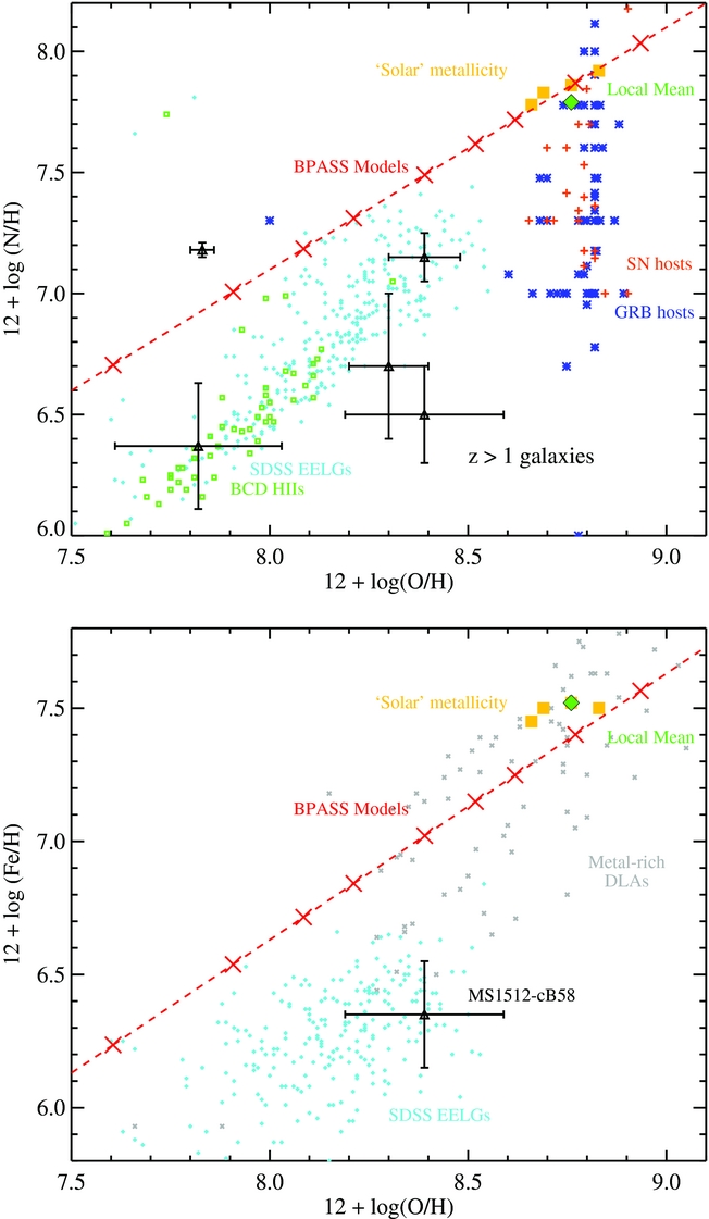
Elemental abundances at ‘Solar’ metallicity.
Abundances are given in the form of 12+log(X n /H) where X n is the atomic species in question. NP12 indicates the mean abundances of B type stars in the Solar neighbourhood measured by Nieva & Przybilla (Reference Nieva and Przybilla2012). The last three lines give the values corresponding to Solar in our stellar models and the corresponding atmosphere models. Sources: GS98—Grevesse & Sauval (Reference Grevesse and Sauval1998), GAS07—Grevesse, Asplund, & Sauval (Reference Grevesse, Asplund and Sauval2007), AGSS09—Asplund et al. (Reference Asplund, Grevesse, Sauval and Scott2009), CLSFB10—Caffau et al. (Reference Caffau, Ludwig, Steffen, Freytag and Bonifacio2011).
Abundances of distant galaxies and galaxy composites.
Values are reported in the form 12+log(X n /H) where X n is the atomic species in question. Sources: a BX418, Erb et al. (Reference Erb, Pettini, Shapley, Steidel, Law and Reddy2010), b Lynx arc, Villar-Martín, Cerviño, & González Delgado (Reference Villar-Martín, Cerviño and González Delgado2004), c 8 o’clock arc, Dessauges-Zavadsky et al. (Reference Dessauges-Zavadsky, D’Odorico, Schaerer, Modigliani, Tapken and Vernet2010), d SGAS J105039.6+001730, Bayliss et al. (Reference Bayliss, Rigby, Sharon, Wuyts, Florian, Gladders, Johnson and Oguri2014), e MS 1512-cB58, Pettini et al. (Reference Pettini, Rix, Steidel, Adelberger, Hunt and Shapley2002), f the KBSS-LM1 composite galaxy template of Steidel et al. (Reference Steidel, Strom, Pettini, Rudie, Reddy and Trainor2016)—we use the nebular gas metallicities; g CASSOWARY20, James et al. (Reference James2014), h GRB 130606A afterglow, Hartoog et al. (Reference Hartoog2015), i GRB 120327A afterglow, D’Elia et al. (Reference D’Elia2014).
Of more significance is the role of iron, as this is the element which is responsible for most opacity in a stellar interior and for driving the surface stellar winds. In our models, the true Solar metallicity can be considered to be represented by either our Z = 0.014 and 0.020 models, which we define as having 12+log[O/H] values of 8.7 to 8.8, with the higher metallicity model having a Solar iron abundance, while the lower metallicity models have a composition more similar to the local Cosmic abundances defined by Nieva & Przybilla (Reference Nieva and Przybilla2012) but are slightly less iron rich. Simultaneous observations of oxygen and iron abundances for galaxies are difficult to obtain in the distant Universe, since iron measurements are typically obtained from weak absorption features in the rest-ultraviolet, while oxygen is typically measured from the strong rest-frame optical gas phase emission lines. Nonetheless, measurements from damped lyman-alpha absorption systems suggest that our [Fe/O] abundances track those in the intergalactic medium at high redshifts over a range of metallicities. Agreement with extreme low metallicity star-forming galaxies in the local Universe (derived from SDSS) is less clear, and suggests that we may slightly overestimate iron abundance relative to oxygen at low metallicities.
The composition employed by bpass is consistent with all the atmosphere model spectra we use during the hydrogen-rich phase of evolution. For WR stars, this issue is not quite as important since the light element composition reflects the progress of nuclear burning rather the initial composition. We choose to scale mass-loss rates by metallicity from Z = 0.020 again to be consistent with previous work.
A final uncertainty regarding the role of stellar composition extends to whether the alpha-element to iron-group elements ratio is constant with total metallicity mass fraction. Alpha elements (which are released by core-collapse supernovae) are formed earlier in the lifetime of a stellar population than iron and other metals (which are formed in type Ia supernovae and massive star winds). A higher abundance of alpha-elements might be expected in lower metallicity systems due to their younger typical stellar populations. At the current time, we do not adjust for this as the relative abundance evolution with metallicity is poorly constrained, and is likely heavily dependent on the star-formation history in individual cases, thus showing significant scatter in the baseline relation (e.g. Woodley & Gómez Reference Woodley and Gómez2010). Although metallicities of extragalactic systems are typically measured and quoted in terms of [O/H], this does not always relate directly to [Fe/H] which is what drives the greatest changes in stellar evolution. Therefore, an approach similar to that of Steidel et al. (Reference Steidel, Strom, Pettini, Rudie, Reddy and Trainor2016) and Bowler et al. (Reference Bowler, McLure, Dunlop, McLeod, Stanway, Eldridge and Jarvis2016), whereby diagnostic emission lines are modelled with an alpha-enriched nebular gas emission component, while the stellar population is modelled at the associated iron abundance, should be considered.
We aim to calculate future model sets with more varied compositions, including α-element enhancement, both to more accurately reproduce Galactic composition and those in the high-redshift Universe, but our v2.1 model set provides a single standard abundance model that can be applied across cosmic time and against which variation can be compared.
7.5. Nebula emission, accretion physics, and X-ray binaries
It should be clearly stated that the baseline BPASS models do not include nebula emission from surrounding gas as a default. The response of diffuse interstellar, or even intergalactic, gas to stellar radiation, together with its reprocessing and emission as nebular lines, is a complex topic which has been explored in detail by other authors (e.g. Ferland et al. Reference Ferland, Korista, Verner, Ferguson, Kingdon and Verner1998; Kewley et al. Reference Kewley, Geller and Jansen2004) and in Section 6.3. The introduction of nebular emission is accompanied by a wealth of free parameters defining the gas geometry, density, abundance ratios, temperatures, and thus ionisation state, and depletion onto dust grains. These must be fixed on a case by case basis by analysis of resolved data or emission line ratios, or alternatively a full grid of models, exploring all these free parameters must be compared to the data. We recommend that our stellar population models be reprocessed by a radiative transfer code such as cloudy or mappings before comparison with observed data in contexts where the nebular effects are expected to be significant (see Section 6.3 above, Xiao & Eldridge Reference Xiao and Eldridge2015, and Xiao et al. Reference Xiao2017). Stanway et al. (Reference Stanway, Eldridge, Greis, Davies, Wilkins and Bremer2014) also explores this issue in more detail.
We also currently do not include the accretion luminosity from X-ray binaries in our model populations since accretion physics is beyond the scope of our models. This can be significant at lower metallicities as the typical black hole mass in our populations increases; therefore, our predictions for ionising fluxes should be considered as a lower bound without this included. While accretion events are short lived, they are also extremely luminous and so may have an appreciable effect on the integrated spectrum of a stellar population in any given time bin. We would thus expect that once an accurate model of accretion onto compact remnants is included, there will be an extra source of hard ionising radiation within our models. This will lead to models with recently formed black holes possibly taking on some of the observational characteristics of very-low luminosity AGN. We note that our omission of accretion-powered emission includes that of cataclysmic variables and similar sources from our integrated spectra, however CV accretion power would be important only in older population where white dwarfs have had time to form. In those older population, there could be other, possibly more pressing, issues if the lower mass stars, such as post-RGB and post-AGB stars (including binaries in these categories), are not well modelled.
7.6. Wolf–Rayet star inflation
It has been known for some time that matching the hydrostatic stellar models of WR stars to the observed parameters is problematic (see Gräfener et al. Reference Gräfener, Owocki and Vink2012, and references therein). This is mainly due to the star having optically thick stellar winds so it is impossible to see the stellar surface, from where the wind is launched in most cases. Here we use the recommended method outlined by the PoWR team to match our WR models to their atmosphere models (Gräfener et al. Reference Gräfener, Owocki and Vink2012). In addition to this, there is growing evidence that the envelopes of WR stars may be still more inflated than predicted by evolutionary calculations (Sander et al. Reference Sander, Hamann and Todt2012; McClelland & Eldridge Reference McClelland and Eldridge2016). It appears this is only important at near-Solar metallicities but can lead to rather lower stellar temperatures by 0.2 dex. This will impact on predicted line emission from our WR populations, specifically the blue and the red WR bumps, in our spectra and require the use of lower surface gravity models than those currently selected. It is impossible at the current time to evaluate the importance of this effect but future work on modelling resolved and unresolved WR populations may provide the necessary constraints and lead to its implementation in future bpass versions.
7.7. Neutron star and black-hole kicks
In these v2.1 models, we have continued to use our kick model based on the Hobbs et al. (Reference Hobbs, Lorimer, Lyne and Kramer2005) observations of Galactic neutron-star velocities. We determine a velocity at random from Maxwell–Boltzmann distribution with σ = 265 km s−1. For black holes, we assume the same method but reduce the strength of the kick by a factor of 1.4 M⊙/M rem, assuming the distribution represents a momentum distribution for black holes. While there is some evidence to suggest, this is the case (e.g. Mandel Reference Mandel2016) the true scaling is still uncertain.
We have recently been investigating a new model for neutron-star kicks where the kick velocity is related to the ejecta mass of the exploding star (Bray & Eldridge Reference Bray and Eldridge2016). There is some evidence from simulations of core-collapse that this model may be the correct one to apply (Janka Reference Janka2012). Once we obtain better constraints on whether the kick is a match to nature or not, we may switch to this new kick model in future versions of bpass. We are still considering how to extend this kick model to black holes.
An important uncertainty in neutron star and black hole formation is how we estimate the remnant masses. Ours is a relatively simple method but does produce similar island of stability to that found by other authors (Ugliano et al. Reference Ugliano, Janka, Marek and Arcones2012; Sukhbold & Woosley Reference Sukhbold and Woosley2014; Ertl et al. Reference Ertl, Janka, Woosley, Sukhbold and Ugliano2016). This can be seen in Figure 6 of Eldridge & Tout (Reference Eldridge and Tout2004a) where contours of remnant masses for given initial mass and metallicity were predicted. The only way to gain insight into the accuracy of our method will be to study future events where the massive stars are observed to disappear without supernovae as found by Adams et al. (Reference Adams, Kochanek, Gerke and Stanek2017). Further insights will come from modelling the black hole mass distribution arising from future gravitational wave sources (see Eldridge & Stanway Reference Eldridge and Stanway2016), while also using results from gravitational microlensing to determine the black hole mass distribution of single free-floating black holes in the Galaxy (Wyrzykowski et al. Reference Wyrzykowski2016).
7.8. Un- and under-represented stellar types
Certain stars may be missing within our populations. One important class are luminous-blue variable (LBV) stars. There are two reasons we do not have these in our populations. One is that we do not know which models will be observed as LBVs. The evolutionary state of these stars is still somewhat uncertain (Smith et al. Reference Smith, Li, Silverman, Ganeshalingam and Filippenko2011; Smith & Owocki Reference Smith and Owocki2006; Humphreys & Davidson Reference Humphreys and Davidson1994; Humphreys et al. Reference Humphreys, Gordon, Martin, Weis and Hahn2017). Additionally, if they are the result of transient and irregular mass transfer in a binary system, they may not exist within our set of models as discussed above. This is of course something that will be fruitful to study in future.
For lower mass stars, there are limitations in our modelling of AGB stars and the helium flash. In both cases within the evolution code used, it is difficult to evolve through these phases. Therefore, in our single star models, AGB models never form white dwarfs. The models end once the core has grown to the Chandrasekhar mass. In future, we will replace these models with synthetic AGB models (Izzard et al. Reference Izzard, Tout, Karakas and Pols2004) or recalculate the models with more realistic mass-loss rates after second dredge-up. We note however that in our binary populations, many stars do not evolve to the AGB phase due to binary interactions before second dredge-up.
To get around the core helium flash, we have had to make pseudo-evolution models to circumvent this for stars below about 2 M⊙ for our single-star populations. Because of the large number of binary models, we have not yet searched in detail for failed models due to the core helium flash. Most of our efforts have been concentrated on massive stars within our model populations. However in future we will be able to extend the evolution of these low mass stars.
7.9. Low-mass clusters and IMF sampling
Motivated by recent observations, particularly those of the Tarantula Nebula (Sana et al. Reference Sana2012; Doran et al. Reference Doran2013), we have favoured models of a stellar population drawn from an IMF that extends to an upper mass limit of 300 M⊙. However, as discussed by Eldridge (Reference Eldridge2012) and references therein, a fully populated IMF requires a very large initial molecular cloud, a gas cloud with a total mass of only 1000 M⊙, for example, is unlikely to generate even a single 300 M⊙ star, although evidence for a relation between the most massive star in a cluster and its total mass remains unclear (e.g. Andrews et al. Reference Andrews2014; Popescu & Hanson Reference Popescu and Hanson2014). The result is potentially a strong stochasticity in the high-mass stellar population of low mass star-forming regions (i.e. a star of given mass either forms or does not in any given molecular cloud). Since these most massive stars dominate the light at early ages, this can alter the observable properties of the integrated light measured from the population (e.g. Haas & Anders Reference Haas and Anders2010; Doran et al. Reference Doran2013). In common with other stellar population synthesis models, bpass assumes a sufficiently large population of stars is formed that the IMF is fully sampled, and outputs are normalised to a total mass of 106 M⊙. While these should comfortably scale up to larger mass starbursts, we note that caution should be used when studying star-forming regions of significantly lower total mass. For such systems, our equivalent set of data products including an IMF which only samples up to 100 M⊙ may be more appropriate. Note that we do not provide IMFs generated with stochastic sampling since these are heavily dependent on initial presumed total mass.
7.10. Old stellar populations
The majority of observational tests presented in this paper have been for relatively young stellar populations (<1 Gyr). At older ages, bpass binary models remain relatively blue compared to single star populations, and do not reach full quiescence until later (see Figure 5). The reasons why bpass stays blue are two-fold:
The first effect is due to the width of the time bins at late ages and relatively sparse sampling of stellar masses—since each bin is very broad, working with a single age starburst is going to result in all stars in a certain mass range undergoing the bulk of their dramatic evolution in one bin, and not necessarily in adjacent bins. Since there is not an infinite mass resolution in the stellar models, and since stars of different masses die in different ways, that leads to instability in the models at late times—i.e. the behaviour at log(age) = 9.3 might be very different from log(age) = 9.2 or 9.4—this is inherent in the stellar population but also something of a modelling resolution issue and is one we plan to address in future by addition of further stellar models. Some of these fluctuations are also due to our poor estimate of rejuvenation ages for secondary stars where the primary did not explode in a core-collapse supernova. An interim approach is to average several age bins at late ages (effectively degrading the age resolution further, but averaging over some of this stochastic variation). We could also interpolate between initial stellar masses but stellar evolution is non-linear and binary evolution even more so. The best solution to this problem is to increase the number of low-mass stellar models in our grid.
The second issue that needs to be considered is the binary fraction as a function of mass. Since our models were originally tuned to young populations, our focus was on the massive stars, and their binary interaction fraction. This is fixed using a binary period distribution matched to observations (i.e. all the stars in our binary models are technically in binaries, but in many of them the binary is too wide to have any effect on their evolution so they behave like single stars, with the right interacting fraction). However, one thing we have not accounted for systematically (because until recently it has been very poorly constrained by observations, especially as a function of metallicity) is the binary fraction in lower mass stars. The blue colours in our binary models at late ages result to a large extent from interactions between fairly low (~ a few Solar) mass stars and their companions rejuvenating the population. Again, the large time bins are going to make this rather stochastic with some bins more affected than their neighbours. It appears likely our binary models are overestimating the interacting binary fraction in these low mass stars. One reason we also provide the single star models is to provide some capacity to vary the binary fraction by combining the two in proportion, reducing the interaction fraction overall and it might be appropriate to do this incrementally as a function of age (i.e. mass range of dominant stars). Recent work by Moe & Di Stefano (Reference Moe and Di Stefano2017) has provided much tighter constraints on these parameters, although still at Solar metallicity and we are likely to modify our initial binary parameter distributions in future work.
Our single star models perform generally better at late ages, particularly in the ultraviolet and optical but the excess of AGB stars identified in Section 2.4.1 and Figure 7 at late times remains an issue to be explored in future work. Treatment of the pulsating phases of AGB stars is currently neglected, and may have a substantial impact on the survival of such stars and their radii (and hence interactions). While these results are features of the models, rather than necessarily problems in them, we recognise that this can cause significant issues for SED fitting and for measurement of absorption line features such as the Lick indices (Worthey et al. Reference Worthey, Faber, Gonzalez and Burstein1994; Worthey & Ottaviani Reference Worthey and Ottaviani1997). As Figure 45 demonstrates, our binary models fail to reproduce the absorption line indexes observed in old globular clusters within the Milky Way, while these are well fit by our single star populations—as might be expected if the binary fraction in low-mass stars is overestimated. This is not an unambiguous interpretation: the binary fraction in globular clusters may differ from that in the field or extragalactic environments, and more work is needed to clarify the situation. Improved treatment of white-dwarf atmospheres is also likely to improve performance here in future versions, since these can have a pronounced effect on the Balmer line indices.
Lick indices calculated from bpass models at stellar population ages between 1 and 12 Gyr in age, at a variety of metallicities. Data points indicate the indices measured for Galactic globular clusters by Kim et al. (Reference Kim, Cho, Sharples, Vazdekis, Beasley and Yoon2016), adjusted to the original (Worthey et al. Reference Worthey, Faber, Gonzalez and Burstein1994) index scale using the zeropoints given by Schiavon (Reference Schiavon2007). The MgFe50 index was defined by Kuntschner et al. (Reference Kuntschner2010) as insensitive to abundance ratios. In all cases, the single star models perform better than the binary models for these very old stellar populations, as discussed in Section 7.10.
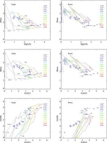
Nonetheless, binary models do offer some interesting prospects for understanding old stellar populations that currently challenge interpretations. An example is the UV-upturn phenomenon in elliptical galaxies with >10-Gyr-old stellar populations (e.g. Dorman, O’Connell, & Rood Reference Dorman, O’Connell and Rood1995). The origin of the ultraviolet emission in these sources is unclear, but is likely associated with a substantial population of helium-rich stars. While it is possible that these systems were formed in regions with helium enhancement (e.g. Chung, Yoon, & Lee Reference Chung, Yoon and Lee2011), that raises questions regarding the origin of such enhancement. An alternative is that they host stars whose atmospheres have been stripped through binary interactions, and a binary model such as bpass is essential for exploring this possibility.
In future, it may be possible to use Lick indices, observations of UV-upturn galaxies and similar data to further constrain the binary model and explore α-enhancement in these models, but at present we do not recommend using our v2.1 binary models to fit populations more than a few gigayears old without due caution.
7.11. Dust and radio components
In common with most other spectral synthesis codes, we do not account for re-emission of extincted light processed into thermal black-body radiation by dust grains (or indeed polyaromatic hydrocarbons). We recommend the use of an energy-balance formalism such as that applied by MAGPHYS (da Cunha, Charlot, & Elbaz Reference da Cunha, Charlot and Elbaz2008) to predict stellar population effects on emission in the infrared and submillimetre (see Stanway et al. Reference Stanway, Levan, Tanvir, Wiersema, Mundell and Guidorzi2015, for an example of this approach). The detailed physics of how binary interactions affect dust must consider supernova and stellar wind dust yields, as well as the destruction of dust grains by energetic events such as supernovae or intense local radiation fields.
Given that bpass is a full stellar population synthesis code, able to make predictions for all phases of stellar evolution and rates of stellar death, it should be possible to implement a dust yield model at a later date, but this is beyond the scope of the current version, and will rely on future resourcing.
Similarly, emission in the radio continuum arises from a combination of thermal and non-thermal components, with the latter believed to track the supernova rate in a stellar population (see e.g. Condon Reference Condon1992; Tabatabaei et al. Reference Tabatabaei2017). While a crude estimate of the time evolution in radio emission can therefore be constructed from the rate of supernovae in current models (see Greis et al. Reference Greis, Stanway, Levan, Davies and Eldridge2017, for preliminary work on this), a detailed treatment again awaits future work.
8 CONCLUSION
In this paper, we have presented the numerical methodology, input models and primary outputs of version 2.1 of the bpass stellar population modelling code. This code builds composite stellar populations from a set of detailed stellar evolution models spanning masses from 0.1–300 M⊙ and at metallicities from 0.05 to 200% of Solar. It combines these with publically available stellar atmosphere models to predict the spectral properties of simple stellar populations at ages from 1 Myr to 100 Gyr. We have addressed its performance in different regimes and presented observational validation tests demonstrating its efficacy, and its limitations, in a wide variety of contexts.
These include the following:
-
1. The physical characteristics and evolutionary state of well-constrained eclipsing binary stars, which are well matched by model predictions.
-
2. The population ratios of different massive stellar types, including massive stars, as a function of metallicity, which are generally consistent with observed ratios across a range of metallicities.
-
3. The Hertzsprung–Russell diagrams and photometric colours of single-aged stellar clusters, which are generally well fit in our models, but suggest caution is needed in fitting old stellar populations, or those dominated by certain rare stellar categories.
-
4. The distribution and properties of compact stellar remnants, which show good agreement between observations and models.
-
5. The rates, progenitors, and characteristics of astrophysical transients, which agree well with observational constraints, but hint that those sources collapsing to black holes may be under-represented in supernova surveys.
-
6. The colours and diagnostic line strengths of WR galaxies, which can be simultaneously fit at moderate stellar population ages. These are somewhat older in our binary models than single star models would suggest.
-
7. The colours of the local star forming galaxy population, which show the difficulty and degeneracy in modelling systems with complex star formation histories and substantial gas nebular or dust components. Models can be found which provide a good fit to the data, but these introduce a large number of tunable free parameters.
-
8. The properties of distant galaxies, including their ionising photon production, optical line ratios, and ultraviolet emission lines, which are generally significantly better fit in our binary models than single star models, and which may be older than single star models suggest, but in which nebular gas again plays an important role.
In the interests of transparency and clarity, we have also discussed key caveats and uncertainties in the models. Some of these, particularly those relating to under-represented rare populations, composition, inflation, and non-stellar components, are present in all stellar population synthesis codes. Others, including period distributions, mass transfer, kicks, and rotational mixing, arise from the increased complexity that is inevitable in the modelling of stellar binary interactions. In particular, we identify several aspects of old stellar populations (>1 Gyr) as problematic in our current model set and a target for future development.
Despite the presence of these uncertainties, the tests described above indicate that our physically motivated minimal assumptions result in a spectral synthesis model set which provides a good description of the extant stellar populations in a broad range of environments, to an extent comparable to, or exceeding, existing single star spectral synthesis models. Given the ever-growing number of observational constraints on extreme stellar populations, and the expected impact of JWST on the observation of low metallicity systems in the distant Universe, the need for such models is likely to grow rather than diminish over coming years, and we aim to continue to develop the bpass model infrastructure in response to improvements both in stellar modelling and observational constraints.
All outputs of the current bpass v2.1 data release can be found at http://bpass.auckland.ac.nz, and are mirrored at http://warwick.ac.uk/bpass.
ACKNOWLEDGEMENTS
This work would not have been possible without use of the NeSI Pan Cluster, part of the NeSI high-performance computing facilities. New Zealand’s national facilities are provided by the NZ eScience Infrastructure and funded jointly by NeSI’s collaborator institutions and through the Ministry of Business, Innovation & Employment’s Research Infrastructure programme. URL: https://www.nesi.org.nz.
JJE acknowledges travel funding and support from the University of Auckland. ERS acknowledges travel funding and support from the University of Warwick. We thank Robert Izzard for helping us to obtain atmosphere models. We acknowledge very many useful and interesting discussions with bpass users and collaborators past, present, and future, too numerous to name. We also thank the referee of this paper for their hard work and constructive input. We note that bpass development began when the PIs were post-doctoral researchers and we thank our previous employers (University of Bristol, University of Cambridge, Queen’s University Belfast, and the Institute d’Astrophysique de Paris) for supporting our use of time on this work. bpass is human-resource limited and further iterations will be dependent on the PIs securing research funding in future years.