


1. Introduction
At its rapidly warming margins (Shepherd and others, Reference Shepherd2020), the Greenland ice sheet (GrIS) is surrounded by (semi-) detached glaciated areas, commonly referred to in the literature as peripheral glaciers (PGs) and ice caps (Rastner and others, Reference Rastner2012; Bjørk and others, Reference Bjørk2018). These are bodies of ice that have different levels of connectivity with the ice sheet: they are dynamically connected, entirely detached, or separated from the ice sheet by well-defined ice divides (Rastner and others, Reference Rastner2012). All PGs in Greenland including those strongly connected to the ice sheet cover an ice area of 89 720±2781 km2 (Rastner and others, Reference Rastner2012), ~12% of the world's total glaciated area (excluding the ice sheets), playing an important role in Greenland's freshwater export. According to Bolch and others (Reference Bolch2013), all glaciers and ice caps (including those with strong but hydrologically separable connections) lost 40.9±16.5 Gta−1 (0.12±0.05 mm SLE) between 2003 and 2008. This is a significant fraction (up to 14 or 20%) of the reported overall mass loss of Greenland and up to 10% of the estimated contribution from the world's glaciers and ice caps to sea-level rise (Bolch and others, Reference Bolch2013). For the same period, Noël and others (Reference Noël2017) estimated a mass loss of 40±16 Gta−1. In a scenario of continued global warming, Greenland's PGs may lose 19–28% (7.5–11 mm) of their volume by 2100 (Machguth and others, Reference Machguth2013).
Despite this significant contribution to global mean sea level, their mass balance (MB) variability and overall thickness distribution have been difficult to quantify on multi-decal timescales, due to an absence of long-term data (Bjørk and others, Reference Bjørk2018). In general, most studies of the GrIS do not separate sea-level rise contributions between PGs and the ice sheet (e.g. gravimetry-based studies, Shepherd and others, Reference Shepherd2020), making it difficult to differentiate if the PGs have already been included in reported global mean sea-level rise estimates (Bolch and others, Reference Bolch2013). This is probably related to issues of the ice-sheet model grid scale and the size of the PGs. Noël and others (Reference Noël2017) addressed this issue, separating the GrIS and all glaciers and ice caps mass loss contribution by using a 1 km surface mass balance (SMB) product, evaluated against in situ and remote-sensing data, and quantify the mass loss of all Greenland's glaciers and ice caps. However, in the study changes in solid ice discharge are assumed to be negligible. The loss of mass from tidewater glaciers to the ocean through frontal ablation (i.e. calving, subaerial and subaqueous frontal melting) is a major component of the mass budget of the GrIS (Cowton and others, Reference Cowton, Sole, Nienow, Slater and Christoffersen2018; King and others, Reference King2018; Mankoff and others, Reference Mankoff2019; King and others, Reference King2020). The 2010 through 2019 average ice discharge through flux gates as estimated by Mankoff and others (Reference Mankoff2019) is nearly 487±49 Gta−1 with King and others (Reference King2020) reporting similar values. Therefore, it is reasonable to assume that frontal ablation will also be a major component of the mass budget of PGs. Frontal ablation fluxes will strongly affect the ice dynamics of PGs and thus are substantial to assess the amount of ice stored in such glaciers and their potential contribution to sea-level rise.
Most regional studies (e.g. Mankoff and others, Reference Mankoff2019; King and others, Reference King2020) estimate ice-sheet wide discharge focusing on outlet glaciers of the ice sheet. Here, we focus on tidewater PGs that are weakly or not connected to the ice sheet (also referred to as just PGs in this study) for which there are no comprehensive regional observations or individual estimates of frontal ablation, and little is known about their calving front geometry. Without comprehensive regional observations or sufficient individual estimates of frontal ablation, constraining model parameters remains a challenging task in this region.
There are volume and ice thickness distribution estimates for PGs that are weakly or not connected to the ice sheet from Farinotti and others (Reference Farinotti2019), where an ensemble of up to five models provided a consensus estimate for the ice thickness distribution of these glaciers (in Greenland only two models participated). Typically, these models use principles of ice flow dynamics to invert for ice thickness from surface characteristics, and some need to estimate ice fluxes from the assumption that they balance the surface mass budget (mass conservation approaches). Recinos and others (Reference Recinos, Maussion, Rothenpieler and Marzeion2019) showed that when ignoring frontal ablation in ice thickness inversion methods based on mass conservation (as listed in Farinotti and others, Reference Farinotti2017), most glacier models may underestimate the regional ice mass stored in tidewater glaciers by ~11–19% in the Alaska region. For individual glaciers, ice volume may be underestimated by up to 30% when ignoring the impact of frontal ablation, independently of the size of the glacier. Only one model in the consensus estimate accounted for frontal ablation of tidewater glaciers (i.e. Huss and Farinotti, Reference Huss and Farinotti2012; Huss and Hock, Reference Huss and Hock2015). However, this model, along with the rest of the ice thickness inversion methods, still suffers from considerable uncertainty associated with the uncertainty about the true frontal ablation values (Recinos and others, Reference Recinos, Maussion, Rothenpieler and Marzeion2019). In projections of glacier mass loss on global and regional scales, the relative importance of glacier model uncertainty decreases over time, but it is the greatest source of uncertainty until the middle of this century (Marzeion and others, Reference Marzeion2020). It is estimated by Huss and Hock (Reference Huss and Hock2015) that frontal ablation accounts for 10% of total global glacier estimates of ablation, but with only one study in the literature accounting for this process at a global scale, more regional and global estimates are needed. Consequently, it is important to investigate not only the ice sheet but also these local tidewater PGs, which cover 25% of the total glaciated area in the region outside the main ice sheet, as shown in Figure 1.
Study area overview. (a) Map with the PG distribution; the different colours indicate the outlines of the PGs classified as land-terminating (grey outlines) and marine-terminating glaciers (dark and light blue outlines) in the Randolph Glacier Inventory (RGI v6.0). Dark blue outlines indicate tidewater glaciers with connectivity level 2 and light blue outlines indicate tidewater glaciers with connectivity levels 0 and 1, which are the focus of this study. Connectivity levels are defined according to the RGIv6.0 connectivity attribute. (b) Fraction of the ice-sheet area covered by each glacier category in percent. (c) Percentage of the study area (light blue in (b)) that can and cannot be modelled by OGGM due to preprocessing errors (brown), gaps in observational data (green, red and pink), or for which no calving value can be determined by the parameterisation (yellow, more details in Section 5).

In this study, we present a regional estimate of mass loss through frontal ablation for most PGs (see study area in Figs 1b, c). We use the Open Global Glacier Model (OGGM v1.3.2, Maussion and others, Reference Maussion2019) updated with the calving parameterisation described in Recinos and others (Reference Recinos, Maussion, Rothenpieler and Marzeion2019) to simulate frontal ablation fluxes for Greenland's tidewater PGs and compute their volume and ice thickness distribution. By accounting for frontal ablation estimates of each individual PG, we not only improve the thickness and volume estimated by OGGM, but also the bedrock topography estimated at the calving front. This allows us to assess how including frontal ablation processes in the model will impact OGGM's estimate of ice stored in PGs. By comparing our estimates to Farinotti and others (Reference Farinotti2019), we then quantify the uncertainty in the PGs volumes when this parameterisation is not included in the glacier models or is poorly constrained.
We do this by calibrating the calving parameterisation in OGGM with three model-independent datasets and via two different methods. The first method calibrates the parameterisation using surface velocity fields derived from satellite observations. For this method we use and compare two different datasets: surface velocities from the MEaSUREs Multi-year Greenland Ice Sheet Velocity Mosaic (MEaSUREs v1.0, Joughin and others, Reference Joughin, Smith, Howat and Scambos2016) and from the ITS_LIVE Regional Glacier and Ice Sheet Surface Velocities Mosaic (Gardner and others, Reference Gardner, Fahnestock and Scambos2019, ITS_LIVE). The second method uses SMB estimates from the monthly output of the polar Regional Atmospheric Climate Model version 2.3p2 (RACMO2.3p2, Noël and others, Reference Noël, van de Berg, Lhermitte and van den Broeke2019), statistically downscaled to 1 km resolution following Noël and others (Reference Noël2016).
Both calibration methods make equilibrium assumptions for the ice dynamics and MB processes. We assume that the average amount of ice that passes through the glacier terminus in a MB year (average frontal ablation flux estimated by the calving law) must be equal to the amount of ice delivered to the terminus (ice flux estimated from the distribution of the mass). By assuming such equilibrium conditions, we estimate parameter values for each individual PG. We (1) compare the difference of parameter values, frontal ablation and calving rate estimates between both calibration methods and all three datasets (MEaSUREs v1.0, ITS_LIVE and RACMO2.3p2) and (2) quantify the effect of accounting for frontal ablation on the first ice thickness estimation of OGGM and on the ice volume and volume below sea level estimates for PGs. By using two different methods of calibrating the model and comparing the output after calibration, we determine at which degree PGs have an equilibrium between their climatic MB and the dynamic discharge of ice into the ocean. If the results of both calibration methods were to be the same for a particular PG, we could assume that the glacier's solid ice discharge (best represented by calibrating the model with velocity observations) is in equilibrium with the glacier's climatic MB (best represented by the second method and the RACMO SMB data).
2. Input data and pre-processing
2.1. Glacier outlines and local topography
We use the glacier outlines defined in the region 5 of the Randolph Glacier Inventory (RGI v6.0, Pfeffer and others, Reference Pfeffer2014). We only include in our simulations glaciers that are classified as marine-terminating glaciers (also referred to as tidewater glaciers in this study) with a weak or no connection to the ice sheet (see map in Fig. 1). Those are glaciers with a level of connectivity 0 and 1 in the RGI attributes (Rastner and others, Reference Rastner2012). From these outlines, only one entity has been manually modified. Flade Isblink Ice Cap (RGI ID no. RGI60-05.10315) is located in North-East Greenland (see Fig. 2a). In the RGI v6.0, this ice cap is a single glacier entity not subdivided into basins and is classified as a whole as marine-terminating (Fig. 2a). An improved outline was provided by Philipp Rastner (pers. comm.), containing individual drainage basins. It was processed using the ArcticDEM topographic data (Porter and others, Reference Porter2018) resampled to 25 m resolution (Fig. 2b). We manually identified the tidewater basins using a combination of different velocity fields from the MEaSUREs Multi-year Greenland Ice Sheet Velocity Mosaic, v1.0 (Joughin and others, Reference Joughin, Smith, Howat and Scambos2016) and the ITS_LIVE Regional Glacier and Ice Sheet Surface Velocities Mosaic (Gardner and others, Reference Gardner, Fahnestock and Scambos2019, ITS_LIVE). Flade Isblink Ice Cap features several water-terminating basins but according to velocity observations only six are active calving basins shown as red outlines in Figure 2c.
Flade Isblink Ice Cap outlines (black and red lines), topography and surface velocity (colour maps). (a) Original outline from the RGIv6.0. (ID RGI60-05.10315). (b) Subdivided outline processed using ArticDEM data and velocity fields from the Greenland 250 m velocity mosaic (Joughin and others, Reference Joughin, Smith, Howat and Scambos2016). (c) Velocity fields over the ice cap. The active tidewater basin outlines are highlighted in red.

In OGGM, a local map projection is defined for each glacier entity in the inventory following the methods described in Maussion and others (Reference Maussion2019). We use a Transverse Mercator projection centred on the glacier. Then, topographical data are selected automatically and interpolated to the local grid. All DEMs are re-sampled to a resolution depending on the glacier size (Maussion and others, Reference Maussion2019) and smoothed with a Gaussian filter of 250 m radius.
For Greenland, OGGM uses the Greenland Mapping Project (GIMP) DEM (data acquisition: 2003–09, resolution: 90 m, Howat and others, Reference Howat, Negrete and Smith2014) as default. However, in this study, for most of the glaciers we use the ArcticDEM (data acquisition: 2007–18, resolution: 100 m, Porter and others, Reference Porter2018) since the GIMP DEM quality imposed errors in some of the automated glacier centreline identification and therefore errors in the calving front geometry estimation (more details in Section 2.2). For those glaciers where there are gaps in the ArcticDEM, we use GIMP to increase area coverage.
2.2. Glacier flowlines, catchment areas and widths
The glacier centrelines are computed following an automated method based on the approach of Kienholz and others (Reference Kienholz, Rich, Arendt and Hock2014). The centrelines are then filtered and interpolated to a constant grid spacing (see Fig. 3a). The geometrical widths along the flowlines are obtained by intersecting the normals at each gridpoint with the glacier outlines and the tributaries’ catchment areas. Each tributary and the main flowline has a catchment area, which is then used to correct the geometrical widths (see Fig. 3b). This process assures that the flowline representation of the glacier is in close agreement with the actual altitude-area distribution of the glacier. The width of the calving front, therefore, is obtained from a geometric first guess, which may lead to uncertainties in the frontal ablation computations as shown in Recinos and others (Reference Recinos, Maussion, Rothenpieler and Marzeion2019). Uncertainties in the terminus geometry can in this case be compensated by calibrating the calving constant of proportionality k with observations (see Sections 3.3 and 4).
Input data and preprocessing steps using the glacier with ID RGI60-05.00800 as an example (red dot in the Greenland map). (a) OGGM topographical data preprocessing and computation of the flowlines. (b) Flowlines width correction according to the glacier catchment areas and altitude-area distribution. (c) OGGM thickness distribution differences between accounting and not accounting for frontal ablation in the MB model (e.g. q calving = 0.24 Gta−1). (d) MEaSUREs Greenland 250 m velocity mosaic. (e) ITS_LIVE Greenland 120 m velocity mosaic. (f) SMB mean over 1960–90, from the Regional Atmospheric Climate Model RACMO2.3p2, downscaled to 1 km. (g and h) Velocity data re-projected to the glacier grid. (i) SMB mean over 1960–90, from the Regional Atmospheric Climate Model RACMO2.3p2, downscaled to 1 km and re-projected to the glacier grid.

2.3. OGGM climate data and SMB observations
The MB model implemented in OGGM (Section 3.2) uses monthly time series of temperature and precipitation. The current default is to use the gridded time-series dataset CRU TS v4.01 (Harris and others, Reference Harris, Jones, Osborn and Lister2014), which covers the period of 1901–2015 with a 0.5° resolution. In OGGM we take this raw, coarse dataset and downscale it to a higher resolution grid (CRU CL v2.0 at 10′ resolution, New and others, Reference New, Lister, Hulme and Makin2002), following the anomaly mapping approach described in Maussion and others (Reference Maussion2019). This provides OGGM with an elevation-dependent climate dataset from which the temperature and precipitation at each elevation of the glacier are computed, and then converted to the local temperature according to a temperature gradient (default: 6.5 K km−1). No vertical gradient is applied to precipitation, but a correction factor p f = 2.5 is applied to the original CRU time series (Maussion and others, Reference Maussion2019; Recinos and others, Reference Recinos, Maussion, Rothenpieler and Marzeion2019). This correction factor can be seen as a large-scale correction for orographic precipitation, avalanches and wind-blown snow. It must be noted that this factor has little (if any) impact on the MB model performance in terms of bias but might lead to larger uncertainties on MB profiles, mass-turnover in the glacier and therefore also frontal ablation. The MB model (including the p f, see Section 3.2) is calibrated with direct observations of the annual SMB. For this, OGGM uses reference SMB data from the World Glacier Monitoring Service (WGMS, 2017).
2.4. Surface velocity observations
We use two different satellite-derived velocity products to calibrate the calving parameterisation. We use surface velocity fields derived from the MEaSUREs Multi-year Greenland Ice Sheet Velocity Mosaic, v1.0 (Joughin and others, Reference Joughin, Smith, Howat and Scambos2016) at 250 m resolution. These data were collected between 1995 and 2015 and cover most of Greenland as shown in Figure 3d, only 3% of the study area (1007.41 km2) has no data coverage (see Fig. 1c). We also use surface velocity fields derived from the ITS_LIVE Regional Glacier and Ice Sheet Surface Velocities Mosaic (Gardner and others, Reference Gardner, Fahnestock and Scambos2019, ITS_LIVE) at 120 m resolution. These data were collected between 1985 and 2019 and cover most of Greenland (see Fig. 3e), only 5% of the study area has no data coverage (1786.08 km2). According to the ITS_LIVE data documentation, velocities are given in ground units (i.e. absolute velocities). Therefore, we use bilinear interpolation to re-project the velocities to the local glacier map by re-projecting the vector distances (see Fig. 3h).
For each glacier and for each dataset (MEaSUREs and ITS_LIVE), a subset of velocity estimates and their errors are computed by interpolating the main flowline coordinates onto the glacier velocity raster grid (shown in Figs 3g, h) using the nearest-neighbour method. We calculate the mean surface velocity at the lowest one third section of the main flowline and use this value to compare with model-derived velocities (see more in Section 4.1). We also extract from the uncertainty mosaics the mean velocity error for the same section of the flowline. We focus on the last one third of the flowline to ensure that even if there are data gaps right at the calving front, we still obtain a reasonable estimate of average velocity close to the front.
2.5. SMB from RACMO
We use output of RACMO2.3p2 at 5.5 km (Noël and others, Reference Noël, van de Berg, Lhermitte and van den Broeke2019), statistically downscaled to 1 km resolution following Noël and others (Reference Noël2016), to calibrate and validate the model. In brief, the model covers the period 1958–2018, and incorporates the dynamical core of the High Resolution Limited Area Model and the physics from the European Centre for Medium-Range Weather Forecast-Integrated Forecast System (ECMWF-IFS cycle CY33r1). RACMO2.3p2 includes a multilayer snow module that simulates melt, water percolation and retention in snow, refreezing and runoff. The model also accounts for dry snow densification, and drifting snow erosion and sublimation. Snow albedo is calculated on the basis of snow grain size, cloud optical thickness, solar zenith angle and impurity concentration in snow (Noël and others, Reference Noël, van de Berg, Lhermitte and van den Broeke2019). RACMO2.3p2 is described in Noël and others (Reference Noël2018), no model physics has been changed. However, increased horizontal resolution of the host model, i.e. 5.5 km instead of 11 km previously, better resolves gradients in SMB components over the topographically complex ice-sheet margins and neighbouring PGs and ice caps (Noël and others, Reference Noël, van de Berg, Lhermitte and van den Broeke2019). RACMO does not estimate frontal ablation but provides an independent estimate of the PG's SMB. RACMO SMB has been extensively evaluated in Noël and others (Reference Noël, van de Berg, Lhermitte and van den Broeke2019), by using accumulation measurements from stakes, firn pits, cores and airborne radar campaigns in the GrIS accumulation zone, as well as 1073 ablation measurements from 213 stake sites (for more details see Noël and others, Reference Noël, van de Berg, Lhermitte and van den Broeke2019). According to Noël and others (Reference Noël, van de Berg, Lhermitte and van den Broeke2019), RACMO at 1 km resolution resolves SMB patterns over narrow glaciers and marginal ablation zones. As shown in Figures 3f, i, the data cover the majority of PGs and its time resolution allows us to compute a glacier-wide SMB mean over several decades (e.g. 1960–90). Only 0.3% of the study area (104.68 km2) has no data coverage (see Fig. 1c). For each RGI entity, a glacier-wide SMB mean is estimated by generating a region of interest; all gridpoints outside the glacier outline are masked out (as shown in Fig. 3i) and a mean over all the pixels inside the glacier outline is computed. This SMB estimate is then used to calibrate the calving parameterisation as explained in Section 4.2. In this study we use the state-of-the-art RACMO SMB for model calibration and evaluation.
3. Open Global Glacier Model (OGGM)
The mathematical framework of the Open Global Glacier Model (OGGM v1.3.2, Maussion and others, Reference Maussion2019) and the frontal ablation parameterisation have been explained in detail by Maussion and others (Reference Maussion2019) and Recinos and others (Reference Recinos, Maussion, Rothenpieler and Marzeion2019). However, in order to understand the calibration methods described in Section 4, we hereby summarise the ice thickness inversion, MB and frontal ablation modules.
3.1. Ice thickness
The ice thickness inversion scheme relies on a mass-conservation approach similar to that of Farinotti and others (Reference Farinotti, Huss, Bauder, Funk and Truffer2009), and is fully automated. The ice thickness is computed from mass turnover and the shallow ice approximation along multiple flowlines.
The flux of ice q (m3 s−1) through a glacier cross section of area S (m2) is defined as:

with $\bar {u}$ being the average cross-sectional velocity (m s−1). Following the approach described in Maussion and others (Reference Maussion2019), q can be estimated from the MB field of a glacier. If u and q are known, S and the local ice thickness h (m) can also be computed by making some assumptions about the geometry of the bed and by solving Eqn (1). The default in OGGM is to assume a parabolic bed shape (S = (2/3) hw) for valley glaciers (unless the section touches a neighbouring catchment or neighbouring glacier via ice divides, computed from the RGI) and a rectangular bed shape (S = hw, with w being the glacier width) for ice caps. For the last five gridpoints of tidewater glaciers, the bed shape is assumed to be rectangular.
By applying the well-known shallow-ice approximation (Hutter, Reference Hutter1981, Reference Hutter1983; Oerlemans, Reference Oerlemans1997; Cuffey and Paterson, Reference Cuffey and Paterson2010) and making use of the Glen's ice flow law, u can be computed as:

with A being the ice creep parameter (which has a default value of 2.4×10⁻²⁴ s−1 Pa−3), n the exponent of Glen's flow law (default: n = 3) and τ the basal shear stress defined in OGGM as:

with ρ the ice density (900 kg m−3), g the gravitational acceleration (9.81 m s−2) and α the surface slope (computed along the flowline). Optionally, a sliding velocity u b can be added to the deformation velocity (u) to account for basal sliding, using the following parameterisation (Budd and others, Reference Budd, Keage and Blundy1979; Oerlemans, Reference Oerlemans1997):

with f s a sliding parameter (default: 5.7×10⁻²⁰ s−1 Pa−3).
Equation (1) becomes a polynomial in h of degree 5 with only one root in R +, easily computable for each gridpoint. The equation varies with a factor 2/3 depending on whether one assumes a parabolic (S = (2/3) hw) or rectangular (S = hw) bed shape (see Maussion and others, Reference Maussion2019; Recinos and others, Reference Recinos, Maussion, Rothenpieler and Marzeion2019, for more details).
3.2. Mass balance
OGGM's MB model is an extension of the model proposed by Marzeion and others (Reference Marzeion, Jarosch and Hofer2012) and adapted in Maussion and others (Reference Maussion2019), to calculate the MB of each flowline gridpoint for every month, using the CRU climatological series as boundary condition. The equation governing the MB is that of a traditional temperature index melt model. The monthly MB m i at elevation z and time-step i is computed as:

where $P_i^{\rm {solid}}$ is the monthly solid precipitation, p f a global precipitation correction factor, T i the monthly temperature and T melt is the monthly mean air temperature above which ice melt is assumed to occur (default: − 1°C). Solid precipitation is computed as a fraction of the total precipitation: 100% solid if T i ≤ T solid (default: 0 °C), 0% if T i ≥ T liquid (default: 2°C), and linearly interpolated in between. The parameter μ* indicates the temperature sensitivity of the glacier, and it needs to be calibrated.
The μ* calibration consists of searching a 31 year climate period in the past, during which the glacier would have been in equilibrium while keeping its modern-time geometry (a geometry fixed at the RGI outline's date), implying that the MB of the glacier during that period in time m 31(t) is equal to zero.
By assuming that m 31(t) = 0, OGGM calculates hypothetical μ candidates for each year t, following Eqn (5). For each μ(t) candidate, the model compares the MB observations (WGMS SMB time series from Section 2.3) and the model-derived MB (m 31(t)). A climatic period, centred at a year t*, is determined where the bias of m 31(t) relative to observations is the smallest. t* is then interpolated to nearby glaciers with no MB observations, to estimate their μ* = μ(t*).
During OGGM MB calibration of μ*, only land-terminating glaciers are considered to find the correct climatic period t*, since the approximation of a closed surface mass budget (m 31(t*) = 0) cannot be extended to tidewater glaciers. For such glaciers, a steady state implies that:

with m 31(t*) being the glacier-integrated MB computed for a 31 year period centred around the year t* (e.g. t* = 1973 for some glaciers in Greenland) and for a constant glacier geometry fixed at the RGI outline's date. q calving is the average amount of ice that passes through the glacier terminus in a year, for a glacier in equilibrium with the climate forcing. ρ is the ice density and A RGI is the RGI glacier area. The steady state assumption of Eqn (6) has direct consequences for the calibration of the temperature sensitivity parameter μ* (for more information see section 3.3 or refer to Recinos and others, Reference Recinos, Maussion, Rothenpieler and Marzeion2019).
3.3. Calving law
The annual mean frontal ablation flux q calving (km3a−1) is computed as a function of the height (h f), width (w) and estimated water depth (d) of the calving front, following the approach of Oerlemans and Nick (Reference Oerlemans and Nick2005) and Huss and Hock (Reference Huss and Hock2015):

where k is a proportionality constant (which needs to be calibrated, see Section 4) with a default value of 0.6a−1 after the results from Recinos and others (Reference Recinos, Maussion, Rothenpieler and Marzeion2019). The water depth (d) is estimated from the free-board, using elevation of the glacier surface at the terminus (E t), and ice thickness (h f) data obtained from the model output:

where z w is the elevation of the water body with respect to sea level. The water depth (d) is estimated using the terminus elevation (E t) obtained by projecting the RGI outline onto the DEM (i.e. the terminus elevation is assumed to be the top of the calving front). d is the bed elevation with respect to sea level and for tidewater glaciers, z w is set to 0 m a.s.l. (for lake-terminating glaciers, it would be the level of the lake surface). However, sometimes there are problems with the DEM's quality at the calving front and the glacier terminus elevation has unrealistic heights. Ma and others (Reference Ma, Tripathy and Bassis2017) showed that shear failure at the calving front limits the ice thickness at the terminus to be $\lesssim$ 150 m above the water line. These bounds compare well with observed water depth and ice thickness combinations detected in Greenland glaciers and deduced theoretically by Bassis and Walker (Reference Bassis and Walker2012), showing that there is a limit of allowed ice thickness and water depth combinations for specific glaciers. Thick glaciers must terminate in deep water to stabilise the calving front, yielding a predicted maximum ice cliff height that increases with increasing water depth (Bassis and Walker, Reference Bassis and Walker2012). Therefore, based on these limits and arbitrary considerations, we impose a minimum of 10 m and a maximum of 50 m height for the glacier freeboard during the thickness inversion. This choice is a compromise between physical plausibility and manual correction of erroneous outlines and DEMs.
We solve for the ice thickness by prescribing that the amount of ice calved (q calving) must be equal to the amount of ice delivered by ice deformation to the terminus calculated in Eqn (1), now referred to as q deformation (see Recinos and others, Reference Recinos, Maussion, Rothenpieler and Marzeion2019, for more details about the implementation and limits of the calving parameterisation in OGGM):

q calving varies with h f as a polynomial of degree 2. q deformation is a polynomial in h f of degree 5 (with Glen's flow law exponential constant n = 3), with an extra term in degree 3 if we account for a sliding velocity (see Section 3.1). Equation (9) is therefore a polynomial that can be solved for h f:

We solve the polynomial in Eqn (10) numerically, via bound-constrained minimisation methods (algorithm provided by SciPy, Virtanen and others, Reference Virtanen2020), which leads to a quick convergence. After finding the solution for the frontal ice thickness (h f) and the corresponding frontal ablation flux (q calving with Eqn (7)), we re-calibrate the temperature sensitivity of the glacier μ* with this new flux (see Eqn (5)) and invert for a new ice thickness distribution for the entire glacier. This always results in an adjustment of μ* towards lower values, thus lowering the equilibrium line altitude (ELA) and unbalancing the surface mass-budget, allowing a positive frontal ablation flux. Note that this re-calibration of OGGM MB (m 31) is always necessary (regardless of the choice of model parameters such as k or Glen's A) in order to reconcile mass-conservation and upstream ice thickness with frontal ablation: a problem that presents itself in any glacier model. If no k value satisfies the mass conservation condition of Eqn (9), μ* is fixed to zero and the frontal ablation flux q calving is obtained by closing the mass budget instead of using the calving law (Recinos and others, Reference Recinos, Maussion, Rothenpieler and Marzeion2019). In most cases it is possible to find μ* > 0 compatible with a frontal ablation flux, by calibrating a glacier-specific k value (see Supplementary S2 for more information on the cases where there is no solution to Eqn (9)). This process results always in a larger glacier volume and with a thicker glacier at the terminus as shown in Figure 3c.
4. Calibration of the calving parameterisation
The simple calving law described in Section 3.3 and implemented in OGGM by Recinos and others (Reference Recinos, Maussion, Rothenpieler and Marzeion2019) was calibrated for Alaskan marine-terminating glaciers using regional and individual estimates of frontal ablation of 27 glaciers. However, these types of regional scale estimates do not exist for Greenland.
In the following sections, we present three independent ways to calibrate the calving parameterisation implemented in OGGM via two different methods. We do this by using OGGM-independent data products that focus on very different glacier processes: (1) the ice dynamics and (2) the SMB. We apply OGGM to all glaciers and ice caps in our study region (see Fig. 1) and simulate frontal ablation fluxes and surface velocities (see Section 4.1) by varying the k parameter (see Eqn (7)) within a large range of values (0.01–3.0 a−1). For each k value, we compare the output of the model to (1) satellite velocity observations (from MEaSUREs and ITS_LIVE) and (2) frontal ablation fluxes derived from RACMO2.3p2 SMB means over a reference period (see Section 4.2). This allows us to obtain a calibrated k and associated frontal ablation value per data input for most PGs.
The first method constrains the calving parameterisation using velocity observations, thus frontal ablation fluxes will be consistent with satellite surface velocity observations and their uncertainty. Although the second method uses frontal ablation fluxes derived from RACMO2.3p2 SMB means over an equilibrium reference period, and is based on the strong assumption that most PGs during that time have a balanced budget (i.e. did not experience any mass loss or gain).
According to Fettweis and others (Reference Fettweis2017) the period between 1961 and 1990 has been considered as a period when the total MB of the GrIS was stable (Rignot and Kanagaratnam, Reference Rignot and Kanagaratnam2006) and near zero. Results from all Modèle Atmosphérique Régional simulations (MAR, v3.5.2, Fettweis and others, Reference Fettweis2017) indicate that the years from 1961 to 1990, commonly chosen as a stable reference period for Greenland SMB and ice dynamics, is actually a period of anomalously positive SMB (~ +40 Gta−1) compared to 1900–2010. Reconstructions show that the SMB was particularly positive during those years (SMB was most positive from the 1970s to the middle of the 1990s), suggesting that a mass gain may well have occurred during this period, in agreement with results from Colgan and others (Reference Colgan2015). Noël and others (Reference Noël2017) also estimate for the period of 1958–96 a positive SMB trend (~ +1.11 ±1.62 Gta−2). The mass gain, according to Colgan and others (Reference Colgan2015), might have been only at a certain altitude a.s.l. due to mass being deposited there via ice dynamics (not directly gained via snowfall/accumulation).
Here we assume that most PGs also experienced the same equilibrium conditions and that their SMB should have also been positive, something that we can verify using RACMO SMB estimates (see Section 4.2). More recent studies (e.g. Mouginot and others, Reference Mouginot2019) suggest that PGs were in balance at the beginning of the seventies, and that the SMB of most of the GrIS was positive up until the year 2000. With the exceptions of the Northwest (NW) and Northeast (NE) sections where the SMB becomes slightly negative from 1972. Based on this literature research, we also consider the period from 1961 to 1990 as a stable reference period where we assume that the PGs in our study region were in equilibrium.
Considering an equilibrium between what the glacier gained and calved might not reflect real frontal ablation fluxes but such estimates serve as a base to estimate the dynamic mass loss of glaciers when combined with frontal ablation estimates constrained from velocity observations.
4.1. Method I: constraining k using velocity observations
For this calibration method we compute modelled surface velocities along the main flowline after estimating a glacier thickness distribution per k value. OGGM relies on the shallow ice approximation (as stated in Section 3.1), thus assuming that the ice moves as a laminar flow, meaning that the z-component of the velocity equals zero. The creep relation can be written as Cuffey and Paterson (Reference Cuffey and Paterson2010):

For a constant ice density ρ, the driving stress τ acting on a depth h − h(z) within the glacier, increases linearly from zero at the surface to τbasal at the base. Following the concepts defined in Section 3.1, Eqn (11) can be then written as:

For velocities at the surface, Eqn (12) becomes:

where u b is the basal sliding velocity, estimated in OGGM with Eqn (4) (see Section 3.1). We then estimate surface velocities following Eqn (13), for all the resultant glacier thicknesses h obtained with each k value (see Sections 3.1 and 3.3 for detailed description of h estimation). Similar to the satellite observations, we calculate the model mean surface velocity u s at the lowest one third section of the main flowline and use this value to compare with the satellite velocity estimate described in Section 2.4. Our first calibration step is to select modelled surface velocities (u s) that fall close or within the lower and upper limit of the observations. We then apply a linear fit (purple line in Figs 4a, b) to this selected model data (blue and green dots in Figs 4a, b) and choose the k values that intercept the velocity observations (dash black lines in Figs 4a, b) including the intercepts to the lower and upper errors as shown in Figure 4.
Illustration of the different ways to calibrate the calving constant of proportionality k for the glacier with ID RGI60-05.00800, shown in Figure 3 as an example. (a and b) OGGM surface velocities computed with different k values (blue and green dots). The dashed black lines indicates surface velocity from MEaSUREsv1.0 (a) and from ITS_LIVE (b), with the light grey shading indicating the standard errors as provided on each data product. (c) OGGM frontal ablation fluxes computed with different k values (orange dots). The dashed black line indicates the RACMO-derived frontal ablation estimate and the light grey shading its uncertainty. Crosses in all plots represent the intercepts to velocity observations and RACMO-derived frontal ablation estimate.

4.2. Method II: constraining k values using SMB from RACMO
For this calibration method we compute model frontal ablation fluxes for each k value and compare them with RACMO-derived frontal ablation fluxes. As explained at the beginning of this section, we consider the period from 1961 to 1990 as a stable reference period where the net mass change of the PGs was zero or close to zero and the PG SMB would have been positive. In a tidewater glacier, a closed mass budget will imply that the amount of ice being discharged from the glacier (q calving in Eqn (7)) equals the amount of ice moved downhill via ice dynamic processes (q deformation in Eqn (1)). According to the principles of mass conservation (Eqns (9) and (6)), we can make the following assumption:

where $\bar {m}_{( 1961\rm {-}90) }$ is the RACMO SMB mean over the reference period, converted to flux units (km3a−1) by multiplying by the RGI glacier area (A RGI) and dividing by the ice density (ρ). We use RACMO-derived frontal ablation fluxes ($q_{{\rm calving}, \, \ {\rm RACMO}}$
 ) as a reference and compare them with OGGM-derived frontal ablation fluxes (q calving) computed while varying the k parameter (orange dots in Fig. 4c). Our first calibration step is to select q calving fluxes that fall close or within the lower and upper limit of the $q_{{\rm calving}, \, \ {\rm RACMO}}$
 estimates and only if such values are positive. A RACMO-derived frontal ablation flux can then be estimated, only if this glacier's $\bar {m}_{( 1961\rm {-}90) }$
 is positive. We then apply a linear fit (purple line in Fig. 4c) to these selected q calving and choose the k values that intercept $q_{{\rm calving}, \, \ {\rm RACMO}}$
 fluxes (dashed black line in Fig. 4c), including the intercepts to the lower and upper error of this estimate as shown in Figure 4c. The uncertainty in RACMO $\bar {m}_{( 1961\rm {-}90) }$
 is calculated as the SD of yearly means from the entire time series of the dataset (1958–2018).
Assuming that RACMO $\bar {m}_{( 1961\rm {-}90) }$ equals the glacier mean frontal ablation flux is a meaningless approach if not compared with frontal ablation fluxes derived from constraining the calving parameterisation with velocity observations. The difference between the results from both calibration methods serves as an indication of how strong the dynamic imbalance might have been for PGs during that period in time.
5. Results
We adjust the calving constant of proportionality k in OGGM's calving parameterisation to match satellite velocity observations (from MEaSUREs and ITS_LIVE) and RACMO-derived frontal ablation fluxes ($q_{{\rm calving}, \, \ {\rm RACMO}}$ ) following the calibration methods described in Section 4. After adjusting the k parameter, we obtain a k value and its uncertainty for each PG and data input used for calibration. We then simulate mean frontal ablation fluxes for tidewater glaciers in an equilibrium setting and compute their volume and ice thickness distribution. We are able to simulate between 71 and 84% of the glacierised area of interest (depending on the data input used for the calibration), ~0.3% of the glacierised area has data gaps in RACMO2.3p2, 3% in MEaSUREs v1.0 and 5% in the ITS_LIVE dataset. Another 3% of the study area present errors in the preprocessing stages of OGGM. Approximately 11% of the remaining area has no calving solution for Eqn (9) (see Fig. 1c and Supplementary S2 for an extended discussion regarding these glaciers). Additionally, 12% of the study area has a RACMO $\bar {m}_{( 1961\rm {-}90) }$
 that is below zero, for such glaciers the assumptions in Eqn (14) no longer holds, hence we specify for these PGs a k RACMO and $q_{{\rm calving}, \, \ {\rm RACMO}} = 0$
 .
.
In the following sections we describe the results of (1) comparing k values, frontal ablation fluxes and calving rates obtained by using the different calibration methods and input data and (2) quantify the impact of accounting for frontal ablation on the estimated ice volume and volume below sea level for PGs when using the different calibration methods.
5.1. Comparison between calibration methods
In this section, we only compare results of glaciers that have a valid k parameter when using both calibration methods and glaciers for which the RACMO $\bar {m}_{( 1961\rm {-}90) }$ was not negative.
The frontal ablation fluxes (computed after calibration) obtained using the velocity method (blue and green box plots in Fig. 5b) are on average larger in magnitude than those found using the RACMO method (orange box plots in Fig. 5b). This finding is also true for the calving constants of proportionality (k) but only for glaciers which the area is larger than 50 km2. For the frontal ablation fluxes this result is independent of the glacier size as shown in Figure 5b. However, the difference in fluxes is less significant for smaller glaciers (areas ranging from 0 to 15 km2) and when comparing ITS_LIVE vs RACMO-derived estimates. Figure 5a shows large differences between MEaSUREs-derived k values and the rest. This is probably due to large uncertainties present in the MEaSUREs observed velocities, which poorly constrain this parameter in comparison with the ITS_LIVE data (see Figs 4a, b). For some glaciers, the relationship between the calving constant of proportionality k and model estimates is not perfectly linear (as shown in Fig. 4a). Therefore, it is for such glaciers where the uncertainty on each dataset (and the difference of the time periods they cover) plays an important role during our first calibration step, where we select model data that falls between the upper and lower bounds of the observation (or reference value), before estimating the linear fit shown in Figure 4.
Difference between k values (a), frontal ablation fluxes (b) and calving rates (c) obtained by calibrating OGGM's calving parameterisation with three independent datasets: (1) MEaSUREs v1.0 (blue), (2) ITS_LIVE (green) and (3) RACMO (orange). The x-axis is broken into different glacier size categories. The width of the boxes represents the inter quartile range (IQR) of the data values. The line dividing the boxes represents the median. The whiskers represent the range of values for 99.3% of the data. Points outside this range only contain 0.7% of the values distribution.

Considering that fjord width is known to have a strong influence on the glacier dynamics (Benn and others, Reference Benn, Warren and Mottram2007; Jamieson and others, Reference Jamieson, Vieli, Livingstone, Cofaigh, Stokes, Hillenbrand and Dowdeswell2012; Enderlin and others, Reference Enderlin, Howat and Vieli2013; Carr and others, Reference Carr, Stokes and Vieli2014, Reference Carr2015) we also estimate calving rates (which are independent of the width) for a better comparison between the output of both calibration methods and data input. Calving rates estimated after calibrating the parameterisation with velocity observations from MEaSUREs (blue box plots in Fig. 5c) are significantly larger in magnitude than those found using the rest of the methods. However, on average calving rates constrained using MEaSUREs and ITS_LIVE velocity observations are larger in magnitude than those found using the RACMO method for glaciers which the area is larger than 15 km2.
When comparing the output glacier-by-glacier (see Fig. 6), we find that there is no strong correlation between k values obtained by the different calibration methods (Figs 6a to c), although the correlation between k values constrained by only using velocity observations is slightly stronger (MEaSUREs vs ITS_LIVE, see Fig. 6c) than the correlations shown in Figures 6a, b. However, this correlation coefficient is also affected by the large difference in velocity uncertainty between MEaSUREs and ITS_LIVE (see error bars in Fig. 6c).
Comparison of k values (a–c) and frontal ablation fluxes (d–f) obtained by calibrating OGGM's calving parameterisation with three independent datasets: (1) using MEaSUREs v1.0 surface velocities, (2) ITS_LIVE surface velocities and (3) RACMO-derived frontal ablation fluxes. (a–c) Scatter plot of k parameters. (d–f) Scatter plot of frontal ablation fluxes. Correlation coefficient are also given, all correlations are highly significant at the p < 1 × 10⁻⁵ level. The grey error bars represent each parameters uncertainty.

Frontal ablation fluxes derived after constraining the calving parameterisation with the different methods and datasets present slightly higher correlation coefficients (see Figs 6d to f). There is a strong correlation between frontal ablation fluxes obtained by only calibrating the parameterisation with velocity observations (MEaSUREs vs ITS_LIVE, see Fig. 6f). This shows that q calving estimates after constraining the calving parameterisation with velocity observations are significantly different from those derived with the RACMO method. The ‘real’ calving rate and frontal ablation flux of each glacier is probably best represented by the velocity calibration method. Satellite velocity measurements provide an insight into ice dynamics and reflect the ocean influence over the movement of the ice at the calving front, whereas the second calibration method is based on climatic MB data and the assumption that this climatic MB is exactly stabilised by frontal ablation. This assumption appears not to be true for most of the PGs, where fluxes derived with the velocity method are significantly larger than those fluxes derived with the RACMO method. The differences shown in Figures 5, 6 demonstrate that all tidewater PGs have considerable dynamic mass loss and there is a significant imbalance between their climatic MB and ice dynamics.
5.2. PGs frontal ablation, thickness and volume
We compute the average regional frontal ablation flux after calibrating the calving parameterisation with both methods, and found an average flux of 8.05±3.77 km3a−1 (7.38±3.45 Gta−1) when the parameterisation is constrained by velocity observations and 0.76±0.54 km3a−1 (0.69±0.49 Gta−1) if it is constrained using RACMO-derived frontal ablation fluxes. The uncertainties presented here are SDs of the different model configurations for the k parameter (k values found with the velocity method and RACMO method) including the configurations estimated by finding the intercepts to the lower and upper errors of each data input used for calibration as shown in Figure 4. The RACMO calibration method underestimates the amount of ice passing through the glacier terminus, consequently affecting the glacier volume estimation as shown in Figure 7 (see the difference between the blue, green and orange bars).
Total volume of Greenland's tidewater PGs before (brown) and after accounting for frontal ablation (blue, green and orange), when calibrating the calving parameterisation with three independent datasets: (1) using MEaSUREs v1.0 surface velocities (blue), (2) ITS_LIVE surface velocities (green) and (3) RACMO-derived frontal ablation fluxes (orange). For these three model configurations, we have included error bars for each method. The red bar represents the consensus estimate for these glaciers obtained by Farinotti and others (Reference Farinotti2019). The purple bar represents Huss and Farinotti (Reference Huss and Farinotti2012) contribution to the consensus estimate (red bar). The grey bars represent the total volume below sea level for each volume estimate. The percentage in the top left is the percentage of the study area that has a valid k parameter in all calibration methods. The line pattern in the bars represents the volume and volume below sea level contribution of Flade Isblink Ice Cap.

The data used to constrain the calving parameterisation cover different percentages of the study area as shown in Figure 1c. Therefore, for a better comparison between methods, we only compare in Figure 7 results for glaciers that have a valid k parameter in both calibration methods and among all datasets used in the calibration, that is k values for 347 glaciers covering 78.7% of the study area (here we only report final numbers for this group of glaciers). The coloured bars in Figure 7 correspond to different model configurations, one setting q calving = 0 (brown bars) and three more accounting for frontal ablation and adjusting the k parameter according to the values found by each calibration method (blue, green and orange bars). For these different model configurations, we have included error bars for each method. Additionally we added another two bars to Figure 7, showing the model consensus estimate from Farinotti and others (Reference Farinotti2019) (red bar) and the model result of Huss and Farinotti (Reference Huss and Farinotti2012) (purple bar) for the same 349 glaciers modelled. Results show that by including frontal ablation to the model and calibrating the calving parameterisation, volume estimates for Greenland's PGs increased from 14.47 to 15.84±0.32 mm SLE when using the velocity calibration method and to 14.64±0.12 mm SLE when using the RACMO calibration method. Regional volumes are underestimated by 12% if frontal ablation is ignored and/or if the model only relies on SMB estimates and the assumption of a closed budget to calibrate the calving parameterisation. The consensus estimate from all models compared in Farinotti and others (Reference Farinotti2019) for these glaciers is 16.45 and 16.56 mm SLE for Huss and Farinotti (Reference Huss and Farinotti2012) model contribution, that is 2–11% higher than OGGM results for all model configurations. The difference between the consensus volume and OGGM's model configurations (blue, green and orange bars in Fig. 7) becomes smaller if we remove a single glacier entity from the results: Flade Isblink Ice Cap, represented in Figure 7 by the line pattern in each bar plot. In Farinotti and others (Reference Farinotti2019) and Huss and Farinotti (Reference Huss and Farinotti2012) Flade Isblink Ice Cap remained as a single outline (as shown in Fig. 2a), but subdividing the ice cap can contribute to significant differences in the final ice-cap volume. Model volume estimates tend to follow the well-known volume area scaling rule (see Maussion and others, Reference Maussion2019, Fig. 10 for an example), and the subdivision of this ice cap has a very strong influence as shown in Figure 7, where it is responsible for most of the regional volume (see hashed area). If we remove the ice cap from our analysis, we find that the consensus glacier volumes (red bar) for the remaining glaciers are underestimated by 4% when compared to OGGM results that account for a frontal ablation and use the RACMO calibration method and up to 12% when compared to OGGM results using the velocity method to constrain the frontal ablation parameterisation. Note that the consensus estimate for Greenland's PGs is a composite mean of two models: Huss and Farinotti (Reference Huss and Farinotti2012) (purple bar in Fig. 7) and Frey and others (Reference Frey2014). Only Huss and Farinotti (Reference Huss and Farinotti2012) prescribe a positive net flux at the glacier terminus by reducing the ELA that yields a balanced surface mass budget by a value ΔELAcalving which is separately defined for each RGI region and is not glacier-specific. Therefore, frontal ablation was not explicitly accounted for individual glaciers when estimating the glacier thickness distribution and volume (see Huss and Farinotti (Reference Huss and Farinotti2012) for more details). Thus the model consensus volume estimate for these glaciers still suffers from considerable uncertainties related to (1) the implemented frontal ablation parameterisation or (2) not accounting for frontal ablation at all in the glacier model as in the case of Frey and others (Reference Frey2014) model contribution. Additionally, we also calculate the regional ice volume below sea level for all model configurations (grey bars in Fig. 7) and estimate the sea-level rise contribution for PGs from the glacier mass loss using the same equation described in Farinotti and others (Reference Farinotti2019). We found that by including frontal ablation (and if we remove Flade Isblink Ice Cap in Fig. 7), this contribution increases from 7.71 to 7.77±0.05 mm SLE when using the RACMO calibration method and to 8.13±0.18 mm SLE when using velocity observations to constrain the calving parameterisation. The sea-level rise contributions for these glaciers reported by Farinotti and others (Reference Farinotti2019) and Huss and Farinotti (Reference Huss and Farinotti2012) is 7.16 and 7.45 mm SLE respectively without accounting for Flade Isblink Ice Cap, which makes the exact comparison problematic. Regardless of the ice-cap contribution, these results imply that not accounting for frontal ablation and/or only constraining the parameterisation with SMB estimates and a closed budget assumption will directly impact the estimate of these glacier's potential contribution to sea-level rise.
6. Discussion
In the following section we compare modelled surface velocities computed after the calving parameterisation calibration to surface velocity observations from the MEaSUREs v1.0 and ITS_LIVE datasets.
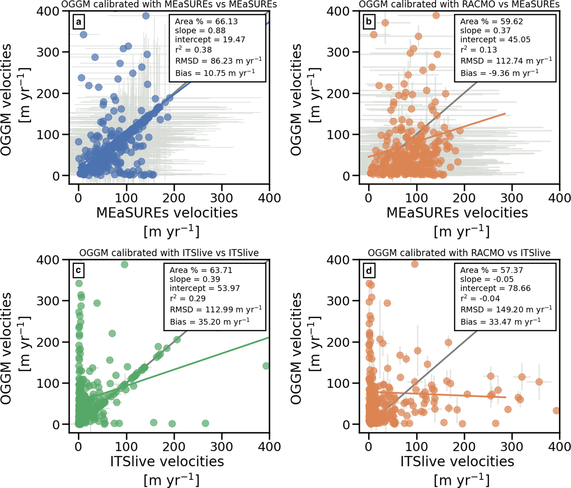
The correlation (r 2) between OGGM velocities and MEaSUREs velocity observations is 0.39, when the calving parameterisation is constrained using that same data input (see Fig. 8a). Figure 8c shows the same analysis but for the ITS_LIVE data. Here, OGGM velocities correlates with the ITS_LIVE velocity observations with a r 2 = 0.29 (the p-values of both correlations are <0.05). These coefficients of determination (r 2) are affected by two aspects: (1) the uncertainty found in the velocity observations (grey error bars in Fig. 8a) which weakly constrained the model in the case of MEaSUREs, and (2) by glaciers which do not present a frontal ablation flux (q calving = 0) after calibrating the k parameter (this occurs in both MEaSUREs and ITS_LIVE results). For a frontal ablation flux to exist (independently of the k value found during the calibration), the model must adjust the SMB and the amount of melt produced along the glacier in order to comply with mass conservation. This is done by modifying the only free unknown parameter in the MB equation: the temperature sensitivity μ* (see Eqn (5)). If even without surface melt (μ* = 0) the total accumulation over the glacier is too small to close the frontal mass budget, the only solution for Eqn (9) for is to have a frontal ablation flux of zero. This can be explained by different factors, generally speaking either that frontal ablation is overestimated (in all k values including those constrained by observations), or that solid precipitation is underestimated. The frontal ablation can be overestimated, e.g. if k and/or the calving law does not represent the dynamics of that particular glacier well, or if h f is overestimated. The discrepancy between acquisition dates among the different input data for the model (e.g. RGI outlines dates, DEM date and velocity observations time span) also contributes to the uncertainty and limitations of our methods to compute a valid k and a realistic frontal ablation flux. By removing glaciers which do not calve after the k calibration, the coefficient of determination (r 2) increases to 0.72 and 0.71 for both datasets (see Supplementary S1 for a detailed explanation regarding non-calving glaciers after the calving parameterisation calibration). As a result of having a q calving = 0 after the calibration, OGGM overestimates the surface velocity for such glaciers as shown in Figures 8a, c. However, for most of the glaciers OGGM is able to estimate a model surface velocity within the uncertainty limit of both observational datasets. Figures 8b, d show the same comparison between modelled and velocity observations from MEaSUREs and ITS_LIVE, but for modelled surface velocities estimated after calibrating the calving parameterisation with the RACMO method, The correlation (r 2) between OGGM velocities and MEaSUREs velocity observations in this case is 0.14 and just 0.04 for the ITS_LIVE data, with this last correlation resulting in a negative r 2. The discrepancy between the results among the two calibration methods (velocity-derived and RACMO-derived estimates), when compared to satellite observations, imply that the model fails to represent individual tidewater glacier dynamics by only constraining the calving parameterisation with SMB estimates and the assumption of a closed budget. Otherwise there should be a better correspondence between velocities derived with both calibration methods and the satellite observations. Note that in Figures 8b, d the percentage of the study area coverage is less (56–58%) than in Figures 8a, c. When using the RACMO method, 12% of the study area has a RACMO $\bar {m}_{( 1961\rm {-} 90) }$ that is below zero. For such glaciers the assumptions in Eqn (14) no longer hold, implying a q calving = 0 for these PGs. Those glaciers (12% of the study area) have been removed from the statistics in Figures 8b, d.
Model performance. (a and c) Comparison of modelled (after calibrating k with the velocity method) and observed surface velocities from (a) MEaSUREs and (c) ITS_LIVE. (b and d) Comparison of modelled (after calibrating k with the RACMO method) and observed surface velocities from (b) MEaSUREs and (d) ITS_LIVE. Regression lines (solid lines) and statistics are shown in the upper right corner, i.e. % of study area represented in the graph, regression slope, intercept, coefficient of determination (r 2), RMSD and bias. The p-values are all <0.05. Grey solid lines represent slopes equal to 1 and intercepts equal to zero and in all scatter plots uncertainty bars are plotted in light grey.
7. Conclusions
We have implemented three independent ways to calibrate the calving constant of proportionality k in OGGM's calving parameterisation and are able to simulate average frontal ablation fluxes for the majority of Greenland PGs that terminate in the ocean. By comparing the model output after applying both calibration methods and constraining the calving parameterisation with three OGGM-independent datasets, we find that the model is not able to predict individual tidewater glacier dynamics if it relies only on RACMO SMB estimates and the assumption of a closed budget to constrain the calving parameterisation. Velocity observations are essential to constrain the model and estimate the dynamic mass loss of PGs. We estimate an average regional frontal ablation flux of 7.38±3.45 Gta−1 after calibrating the model with two different satellite velocity products, and of 0.69±0.49 Gta−1 if the calving parameterisation is constrained using RACMO-derived frontal ablation fluxes. The RACMO calibration method, which is based on climatic MB data and the assumption that this climatic MB is exactly stabilised by frontal ablation, underestimates the amount of ice passing through the glacier terminus, consequently affecting the regional glacier volume estimation and the models capacity to simulate the variance of the velocity observations. Results show that by including frontal ablation to the model and calibrating the calving parameterisation for each individual glacier, volume estimates for Greenland's PGs, increased from 14.47 to 15.84±0.32 mm SLE when using the velocity calibration method and to 14.64±0.12 mm SLE when using the RACMO calibration method. Regional volumes are underestimated by 12% if frontal ablation is ignored and/or if the model only relies on SMB estimates and the assumption of a closed budget to calibrate the calving parameterisation. This change in volume is also reflected on the ice thickness distribution of PGs and hence the regional volume below sea level. Including frontal ablation (if the contribution of Flade Isblink Ice Cap is ignored) increases the sea-level rise contribution for these glaciers, from 7.71 to 7.77±0.05 mm SLE when using the RACMO calibration method and to 8.13±0.18 mm SLE when using velocity observations to constrain the frontal ablation parameterisation. Ignoring frontal ablation and the choice of calibration method will impact the estimate of these glaciers potential contribution to sea-level rise. Velocity observations provide a different insight into the ice dynamic processes of each glacier, and to some extent the influence that the ocean has over the movement of the ice at the calving front. RACMO SMB averaged over a reference period (1961–90) provides an insight into the energy balance of the glacier which is the result of long-term climatic forcing. The discrepancy between the results among the two calibration methods imply that the simulated PGs are losing mass and there is a significant imbalance between their climatic MB and ice dynamics. Additionally our results highlight the importance of subdividing large glacier entities like Flade Isblink Ice Cap into their correct basins to avoid large uncertainties in the regional volume estimate for Greenland PGs.
Supplementary material
The supplementary material for this article can be found at https://doi.org/10.1017/jog.2021.63.
Acknowledgements
BR was supported by the DFG through the International Research Training Group IRTG 1904 ArcTrain. The computations were realised on the computing facilities of the Institute of Geography, University of Bremen. MM acknowledges support of the German Federal Ministry of Education and Research (BMBF) via grant no. 03F0778D. BN is funded by NWO VENI grant VI.Veni.192.019. The OGGM software together with the frontal ablation parameterisation module are coded in the Python language and licensed under the BSD-3-Clause license. The latest version of the OGGM code is available on Github (https://github.com/OGGM/oggm), the documentation is hosted on ReadTheDocs (https://docs.oggm.org/), and the project webpage for communication and dissemination can be found at http://oggm.org. The code and data used to generate all figures and analyses of this paper is available in a permanent DOI repository (https://doi.org/10.5281/zenodo.4757137) as well as the OGGM version used for this study (https://doi.org/10.5281/zenodo.4588404).


 Open access