


1. Introduction
Improved projections of future sea level rise are crucial for adaptation and mitigation efforts. However, mass loss from glaciers and ice sheets is difficult to project due to the complexity of the involved processes (Siegert and others, Reference Siegert, Alley, Rignot, Englander and Corell2020). During the years 2000–2019, glaciers worldwide lost ca. 267 ± 16 gigatons of ice per year, contributing to ca. 20 % of observed global mean sea level rise (Nerem and others, Reference Nerem2018; Hugonnet and others, Reference Hugonnet2021). About 15 % of this mass loss is attributed to frontal ablation (mass loss due to calving, submarine and subaerial frontal melting, and sublimation, as defined by Cogley and others (Reference Cogley2011)) of marine-terminating Northern Hemisphere glaciers (Kochtitzky and others, Reference Kochtitzky2022). Predictions of their future mass loss are afflicted with uncertainties (Edwards and others, Reference Edwards2021) because frontal ablation has hitherto been insufficiently represented in numerical models but is now receiving increased attention (Holmes and others, Reference Holmes, van Dongen and Kirchner2023; Malles and others, Reference Malles2023). While in-situ observations of frontal ablation alongside the development of improved parameterisations of related processes are desirable, remoteness and harshness of the environment in which frontal ablation occurs often limit the collection of relevant data, albeit with notable exceptions (Köhler and others, Reference Köhler2016; How and others, Reference How2019; Holmes and others, Reference Holmes, Kirchner, Kuttenkeuler, Krützfeldt and Noormets2019; Sutherland and others, Reference Sutherland2019).
In recent years, uncrewed aerial vehicles (UAVs) have been used increasingly for glaciological applications in general (Bhardwaj and others, Reference Bhardwaj, Sam, Akanksha, Martín-Torres and Kumar2016), and specifically also for investigations of calving dynamics at marine- as well as freshwater-terminating glaciers (Ryan and others, Reference Ryan2015; Jouvet and others, Reference Jouvet2017; Chudley and others, Reference Chudley, Christoffersen, Doyle, Abellan and Snooke2019; Watson and others, Reference Watson2020; Baurley and others, Reference Baurley, Tomsett and Hart2022; Taylor and others, Reference Taylor, Quincey and Smith2023). This is because UAVs can repeatedly acquire optical imagery, which, when combined with a well-established structure-from-motion photogrammetry process (James and Robson, Reference James and Robson2012; Westoby and others, Reference Westoby, Brasington, Glasser, Hambrey and Reynolds2012), allows for 3D reconstructions of glacier surfaces over time, potentially allowing to detect spatio-temporal changes in frontal geometry. At the same time, UAV missions are commonly limited by short battery lifetimes (reduced further in cold environments) and weight constraints on the scientific payload onboard the UAV. These issues, among others, spur continuous technological development (Jouvet and others, Reference Jouvet2019).
Along calving glacier fronts, some of these limitations may be overcome using uncrewed maritime robots, or, uncrewed surface vehicles (USVs) operating at the sea- or lake surface. For a USV, the operating time and weight of the scientific payload can substantially exceed what is possible for UAVs, implying that USV mapping missions may be expanded beyond their primary typical missions, such as mapping the glacier-proximal sea- or lake floors, the submerged parts of a glacier terminus, and water temperature and salinity profiling (Neal and others, Reference Neal2012; Rignot and others, Reference Rignot, Fenty, Xu, Cai and Kemp2015; Kirchner and others, Reference Kirchner2019; Jackson and others, Reference Jackson2020).
Here, we describe the integration of a photogrammetry payload module into an existing USV, with which mapping missions were conducted at the freshwater calving front of Sálajiegna, Northern Sweden, in September 2022. The work was guided by the hypothesis that USVs represent versatile platforms from which high-resolution photogrammetric products can be derived that will help answer glaciological questions related to changes in frontal geometry and associated volumetric mass loss. Besides describing the advantages and disadvantages of the method, we combine the USV- and UAV-obtained data to get indications of the short-term calving front dynamics at Sálajiegna during its calving season in 2022.
2. Field site
Sálajiegna, a mountain glacier situated on the Swedish-Norwegian border just above the Arctic Circle at about 67°6′ N and 16°25′ E, is the field site for the USV and UAV missions (Figs. 1a–d). In the east, west, and north, Sálajiegna is encompassed by mountains of the Sulitelma massif (also hosting other glaciers, collectively referred to as Sulitjelmaisen). Sálajiegna has an approximate surface area of 24.8 km2 (as deduced from Sentinel 2 optical imagery acquired on 4 September 2022) and ranges in elevation between 869 m and 1750 m a.s.l. The southern margin of Sálajiegna is comprised of two separate glacier tongues, of which the western (Norwegian) is land-terminating, whereas the eastern (Swedish) presently terminates in a proglacial lake at 869 m a.s.l. with an over 1 km long calving front. The lake is not officially named in the Swedish Register of Lakes and Dams (https://vattenwebb.smhi.se/svarwebb), but here it is referred to as Lake Sulitelma. At its highest point, the calving front's western part rises up to 38 m above the lake surface and is hence significantly taller than the eastern part of the front (10-20 m above lake surface). The lake bathymetry along the calving front has been mapped in September 2022 with depths up to 23 m.
(a) and (b) Location of Sulitjelmaisen and Sálajiegna in northern Scandinavia. Glacier areas (blue) are retrieved from the GLIMS database (GLIMS Consortium, 2005). (c) Sálajiegna's glacier front seen on the 0.4 m aerial RGB image by © Lantmöteriet, the Land Survey of Sweden, 24 August 2022. Waypoints for the USV photogrammetric survey along the calving front are indicated with red and blue markers. The black solid line marks the calving front position as of 29 July 2022. (d) Sálajiegna's outline based on Copernicus Sentinel 2 imagery from 4 September 2022, processed by ESA, and legend for (c).
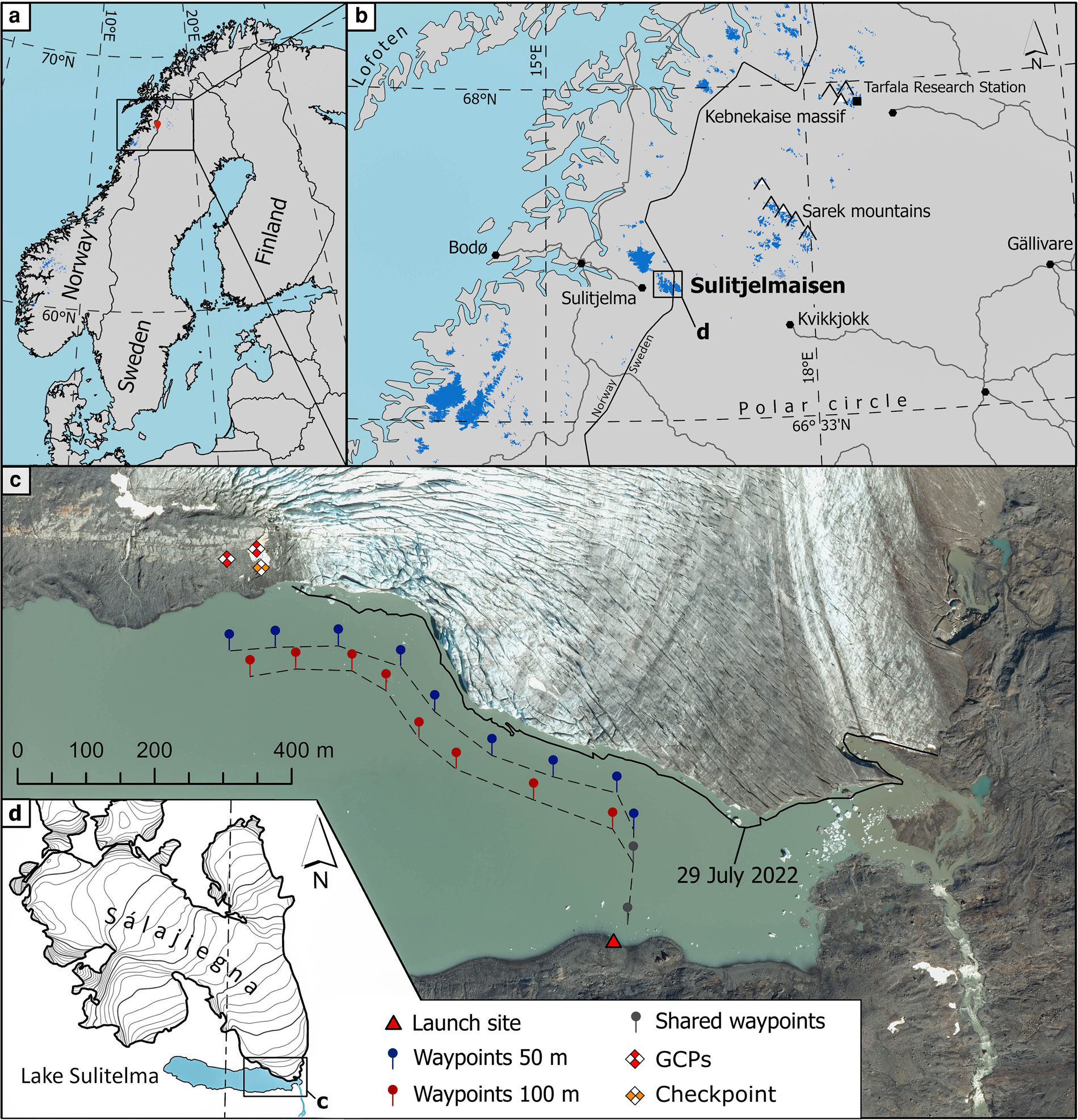
Sálajiegna was one of the first Swedish glaciers for which front position variations were recorded (Westman, Reference Westman1899, Reference Westman1910). From the mid-1960s, front variations of a larger number of Swedish glaciers, including Sálajiegna, were conducted from Tarfala Research Station, Kebnekaise massif (Fig. 1b), in response to a request by the Commission of Snow and Ice (Schytt and others, Reference Schytt, Jonsson and Cederstrand1963). These measurements resulted in a sequence of maps and regular reports to the World Glacier Monitoring Service (Østrem, Reference Østrem1983; Klingbjer and others, Reference Klingbjer, Brown and Holmlund2005; WGMS, 2021). In recent years, Sálajiegna's calving front has appeared to be highly dynamic: In August 2013, for instance, a rapid retreat of its eastern part from its position at the southern lakeshore opened a new drainage path for Lake Sulitelma, leading to an abrupt drainage which lowered the lake level by approximately 10 m (see Appendix A). Knowledge of the event spread mainly in the mountain hiking community, but to our knowledge, not widely beyond (Holmlund, Reference Holmlund2017). This, and an apparent overall rapid retreat has spurred renewed interest in dynamic processes at Sálajiegna, recently investigated in more detail by Hill (Reference Hill2021) and Houssais (Reference Houssais2023).
3. Methods
3.1 USV platform, photogrammetric payload, route planning, and field missions
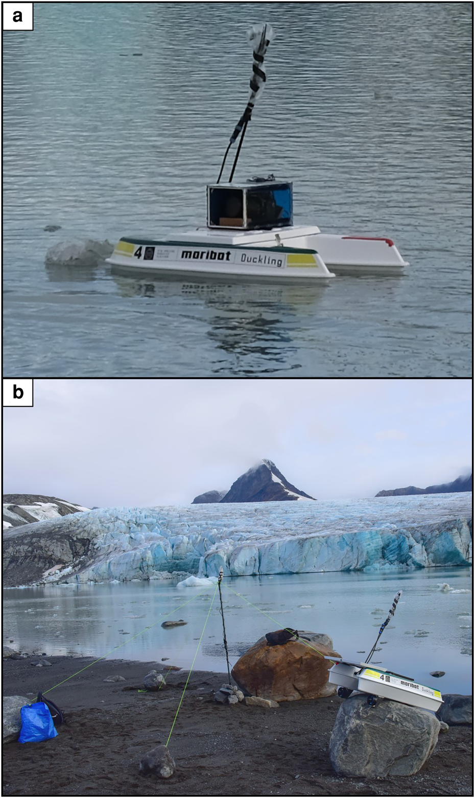
The USV used in this study has been developed at the Centre for Naval Architecture at the KTH Royal Institute of Technology as part of a fleet of maritime robots. The USV is a catamaran with approximate dimensions of 1.12 m (length), 0.73 m (width), and 0.35 m (height) (Fig. 2a). Powered by up to two lithium polymer batteries (each 20 A h at 22.2 V), the USV has an endurance in excess of 6 h, depending on operating conditions and payload. The vehicle is equipped with two thrusters (one on each hull), enabling operation at speeds up to 2.5 m s−1. The vehicle pose, i.e. location and attitude, is provided by a GPS receiver and a motion sensor (attitude and heading reference system, AHRS). The operator can communicate with the USV via radio frequency (RF) at a centre frequency of 900 MHz and radio control (RC) at 2.4 GHz. The standard payload suite consists of an EchoRange Smart SS510 single beam echo sounder for bathymetric mapping of shallow waters. For this study, we have extended the payload suite by a digital single-lens reflex camera and instructed the USV to follow a series of waypoints along Sálajiegna's calving front (Fig. 1c).
(a) The USV in Lake Sulitelma with the photogrammetry setup on top and at (b) the launch site with the antennas, at the shore of Lake Sulitelma (see location in Fig. 1c).
The USV can also be operated in autonomous mode, in which, for example, bathymetric mapping can be performed on a horizontal grid with user-defined mesh sizes. However, in order to accommodate the objective of glacier front photogrammetry and to avoid icebergs and growlers, waypoint-following in combination with manual steering was preferred. For a description of a similar USV from the same above-mentioned fleet of maritime robots operating in autonomous mode during bathymetric mapping of Lake Tarfala, northern Sweden, see Kirchner and others (Reference Kirchner2019).
For the photogrammetric USV survey payload, a waterproof setup including the camera and a Global Navigation Satellite System (GNSS) receiver was developed (Fig. 2). The basis of the setup is a standard acrylic glass box sealed with epoxy. Within the box, a Nikon D810 camera was mounted with the help of velcro tape and kept in place with cork blocks, ensuring a slight upward tilt of the camera such that pictures capture the entire height of the calving front when the USV is in close proximity to the latter. The lens was dialled to 50 mm focal length, and the camera was set to an automatic image capture interval of three seconds. To perform GNSS-assisted triangulation, an Emlid reach M+ single frequency GNSS receiver was directly connected to the camera via the hot shoe adapter. The antenna of the GNSS receiver was mounted on a 12 × 12 cm metal plate on top of the enclosure for better reception. Further, a Raspberry Pi 4 was integrated, enabling remote control of the camera after sealing the watertight enclosure. The GNSS receiver and the Raspberry Pi were powered by a lithium-ion power bank.
USV survey trajectories were planned as a series of waypoints at an approximate distance of 50 m and 100 m from the calving front, based on the terminus position as of 29 July 2022 (Fig. 1c). The pre-planned path could not always be strictly followed due to icebergs obstructing the camera's field of view or the planned track of the USV. With the camera's 35.9 × 24 mm full frame sensor, image dimensions of 7380 × 4928 pixels, and a 50 mm focal length, a theoretical ground sampling distance of 0.48 cm for the 50 m route, and 0.97 cm for the 100 m route, was achieved.
Daily USV photogrammetric surveys of Sálajiegna's calving front were conducted on four consecutive days, 16–19 September 2022, acquiring 559, 454, 476 and 488 images, respectively (Appendix B, Table 4). During all missions, the USV operated at a default speed of 1.25 m s−1 and bathymetric lakefloor mapping was carried out simultaneously.
3.2 UAV photogrammetry field missions
A first UAV photogrammetric survey of Sálajiegna's front was carried out on 29 July 2022 with a DJI Mavic 3, featuring a 1.3 inch camera sensor, image dimensions of 5280 × 3956 pixels, and a 12.29 mm focal length. Because no flight planning software was compatible with this model at the time of the survey, the UAV was flown manually at an altitude of 120 m above the starting point (no terrain follow; approximately 90 to 120 m above the glacier). The camera was set to automatic mode, with a shutter interval of 3 s, while maintaining a cruise speed of 5 m s−1. The chosen parameters result in an overlap of consecutive images of approximately 85 % in the direction of flight. An overlap of images from consecutive flight lines of 66 % was achieved by visually overlapping flight lines with the help of a grid on the controller screen. The combination of the camera and route parameters results in a theoretical ground sampling distance of 3.2 cm. A total of 3093 images were acquired during the survey on 29 July 2022, shortly after the ice on lake Sulitelma had broken up, aiming to capture Sálajiegna's frontal geometry before the onset of the calving season.
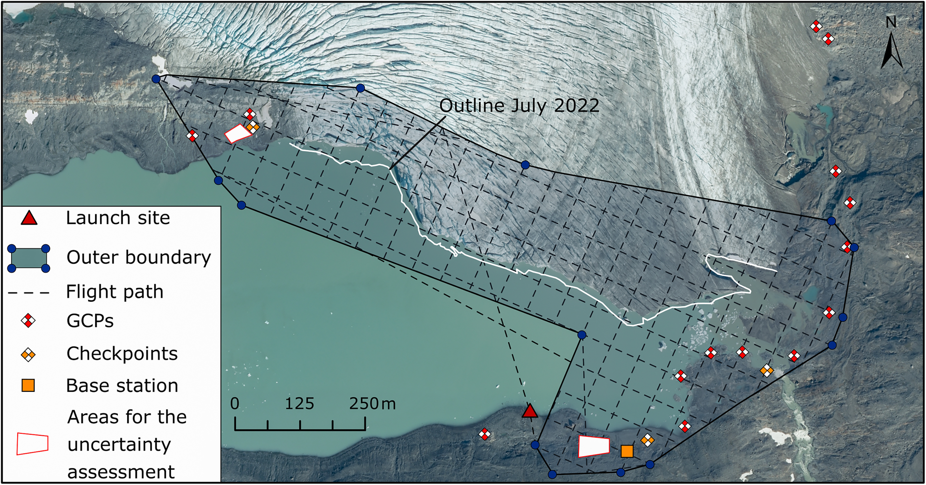
Further UAV surveys were later flown with a DJI Mavic Air 2S for five consecutive days, on 15 September 2022 (860 images acquired) and 16–19 September 2022 (967, 860, 959 and 452 images acquired, respectively), the latter coinciding with USV surveys (Appendix B, Table 4). The UAV's flight path was planned using Dronelink flight planning software. A double grid with 70 % front and side overlap was flown at an altitude of 120 m above the starting point. For each survey, four fully charged batteries (effective battery life during surveys: 22 minutes) were available of which more than three were consumed by the automated flight route, depending on wind conditions. With the remaining battery time, oblique images of the calving front were taken manually. Additional nadir images were taken to ensure all ground control points (GCPs) and checkpoints were covered (Fig. 3). With the UAV's one-inch camera sensor, image dimensions of 5472 × 3648 pixels, and a focal length of 8.38 mm, an approximate ground sampling distance of 3.45 cm was achieved.
Planned UAV flight path of the surveys in September and the resulting coverage area at Sálejiegna terminus. The UAV survey in July had approximately the same southern, eastern, and western extent; however, it expanded northward so that all GCPs on the eastern side were included. The white solid line marks the position of the glacier front as of 29 July 2022 against the background image (0.4 m aerial RGB image by © Lantmäteriet, the Land Survey of Sweden) taken on 14 August 2022. Symbols denoting survey auxiliaries (GCPs), Base station, etc.) are explained in the legend and detailed in section Georeferencing.
3.3 Georeferencing
Two different methods were used to georeference the USV and UAV photogrammetric products. The USV products, on the one hand, were georeferenced by directly geotagging the images with an onboard GNSS receiver. By providing precise camera locations to the photogrammetry software, the need for GCPs is theoretically eliminated. This method is referred to as GNSS-supported aerial triangulation (GNSS-AT) (Benassi and others, Reference Benassi2017; Chudley and others, Reference Chudley, Christoffersen, Doyle, Abellan and Snooke2019). To georeference the UAV products, on the other hand, GCPs were established.
3.3.1 Image geotagging
Due to the difficulty of placing vertical GCPs for the USV in an already challenging proglacial environment, we relied on directly recording precise camera positions, amended by only a few GCPs. We used two Emlid Reach differential carrier-phase GNSS receivers (https://emlid.com/reach), one as a local base station and one as a rover, directly connected to the onboard camera via the hot shoe adapter. The onboard GNSS rover unit was triggered by the camera to record the position at exactly the time of image acquisition. Both the rover and the base station were placed on a 12 × 12 cm metal plate to reduce signal noise. In a post-processing workflow, the collection of GNSS position events was then corrected in RTKLIB (https://rtklib.com) using correction data from the local base station. Finally, the corrected events were matched with the corresponding image using the geotagging tool in Emlid Studio.
The local base station was established by placing one of the GNSS receivers on a bedrock spot, avoiding any topographical barriers that could interfere with signal reception (Fig. 3). Once placed, the device was set to record raw satellite observations from all available satellite systems in the Receiver Independent Exchange Format (RINEX 3.03) at an interval of one second for more than six hours. These were then corrected and averaged in RTKLIB using RINEX 3.03 observations from the Swedish reference station network's (SWEPOS) station in Kvikkjokk, which is nearest to Sálajiegna (approximately 60 km distance), rendering the most accurate position possible of the local base station.
3.3.2 Ground control points and checkpoints
To georeference the UAV surveys, 14 GCPs were established (Fig. 3). Circles with a cross marking the centre were spray-painted onto debris-free bedrock, as close as possible to Sálajegna's calving front. The centre positions were then measured with the same GNSS receiver used as a rover on the USV and further corrected using the local base station in a post-processing workflow in RTKLIB. Additionally, two GCPs were established for the USV surveys (Fig. 1) because it was shown that introducing even just one GCP into a workflow with direct image geotagging can increase georeferencing accuracy (Benassi and others, Reference Benassi2017). These GCPs were placed on near vertical spots to ensure good visibility from the USV.
Further, four checkpoints were established (three for use in the UAV surveys, one for the USV surveys). By revealing possible spatial differences between the location of the checkpoints in the georeferenced model (point cloud) and their measured location, georeferencing and model accuracy can be assessed.
3.4 Structure-from-motion photogrammetry
To create three-dimensional point clouds of Sálajegna's front, a Structure-from-Motion (SfM) and multi-view stereo (MVS) process was applied to all imagery acquired, using the photogrammetry software Agisoft Metashape (version 1.7.6, https://www.agisoft.com). The SfM workflow consists of an image-matching process followed by the estimation of camera locations and camera parameters based on a set of images from different viewing angles (Smith and others, Reference Smith, Carrivick and Quincey2016), resulting in a sparse 3D point cloud for each survey. For georeferencing of the point clouds, the surveyed GCPs were identified and marked on as many images as possible in Agisoft Metashape. All sparse point clouds from UAV and USV surveys were then transformed into dense point clouds by an MVS algorithm, operating directly on pixel scale and hence enabling highly detailed 3D reconstructions (Verhoeven, Reference Verhoeven2011).
Further, the point clouds were filtered based on Agisoft Metashape's point confidence (ignoring all points with a confidence value of less than 4) and also subjected to manual cleaning, especially at the edges and glacier-water interface, as the software fails to produce a level water surface (Bandini and others, Reference Bandini2020).
Finally, the 3D point clouds were subsampled to the same point density and cut to the same extent. The subsampling was performed in MATLAB with the pcdowsample function, which produces 3D grid boxes and averages the location and the normals of all points within this box. The box dimensions were chosen as 5 x 5 x 5 cm. After the subsampling process, the point clouds were imported to CloudCompare, where they were cut to the same extent. Furthermore, any distance between two point clouds caused by georeferencing errors or glacier movement was reduced using the Iterative Closest Point (ICP) algorithm in CloudCompare. From the cleaned dense point cloud, orthomosaics and digital elevation models (DEMs) with a spatial resolution of 10 cm were produced in Agisoft Metashape.
We assess the relative uncertainty of the UAV products by calculating inter-DEM changes in the elevation of bedrock areas, for which no actual change between surveys was assumed, as it has been previously done with UAV products (Chudley and others, Reference Chudley, Christoffersen, Doyle, Abellan and Snooke2019; Jouvet and others, Reference Jouvet2019). The UAV-based DEMs ’ vertical accuracy σ z is calculated as the mean per-pixel standard deviation from the mean elevation of all DEMs. Horizontal accuracy σ xy is given by the root mean square error (RMSE) of velocity fields between 15 and 19 September 2022.
3.5 Detection of calved volumes
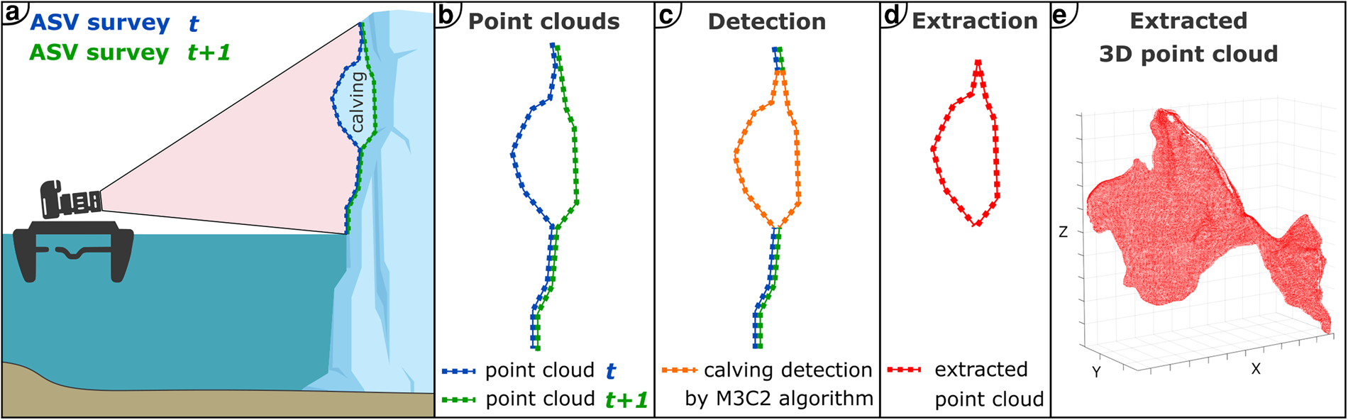
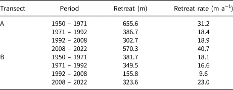
With the USV-obtained data, a detection of geometrical changes along the terminus of Sálajiegna, caused by calving events, was carried out as a change detection between two dense point clouds from consecutive surveys (Fig. 4). For simplicity, we refer to this as calving detection henceforth. The change detection was conducted by applying the Multiscale Model to Model Cloud Comparison (M3C2) algorithm (Lague and others, Reference Lague, Brodu and Leroux2013), implemented in CloudCompare. M3C2 does not rely on meshing or gridding; instead, it operates directly on the point clouds, which makes it especially suitable for photogrammetry or laser scanning products (DiFrancesco and others, Reference DiFrancesco, Bonneau and Hutchinson2020). M3C2 calculates local distances between point clouds while considering surface orientation, implying that change can be detected not only along a specific axis but also in the direction orthogonal to a local surface. This allows a change detection, for instance, in overhanging parts of the glacier front, and makes M3C2 an interesting alternative to DEM of difference (DoD) approaches (Williams, Reference Williams2012). The M3C2 calculations result in a point cloud with distance values to the respective reference point cloud. Positive changes (the glacier front is farther away from the USV than previously) are associated with calving activity, while negative changes (the glacier front is closer to the USV than previously) are associated with glacier advance. Following the M3C2 distance calculation, distinct calving areas were isolated from the rest of the point cloud by extracting all points with a positive distance greater than 0.2 m that were also not connected to any other patch of detected change (Fig. 4). This threshold was chosen to avoid possible erroneous calving detections, as frontal changes can, for example, also be induced by glacier flow. Areas with distance changes below the threshold value are not considered calving areas. Following the calving detection, we categorised calving events based on their location on the calving front. The front was divided into four sectors (I-IV) based on front height, degree of crevassing, and flow velocities.
2D schematics illustrating the extraction of points indicating a calving event. (a) Consecutive USV surveys capture pre- and post-calving conditions. (b) The resulting consecutive point clouds. (c) Detection of areas where calving has taken place. (d) Extraction of points encompassing the calved volume from the point cloud. (e) Example of an extracted 3D point cloud.
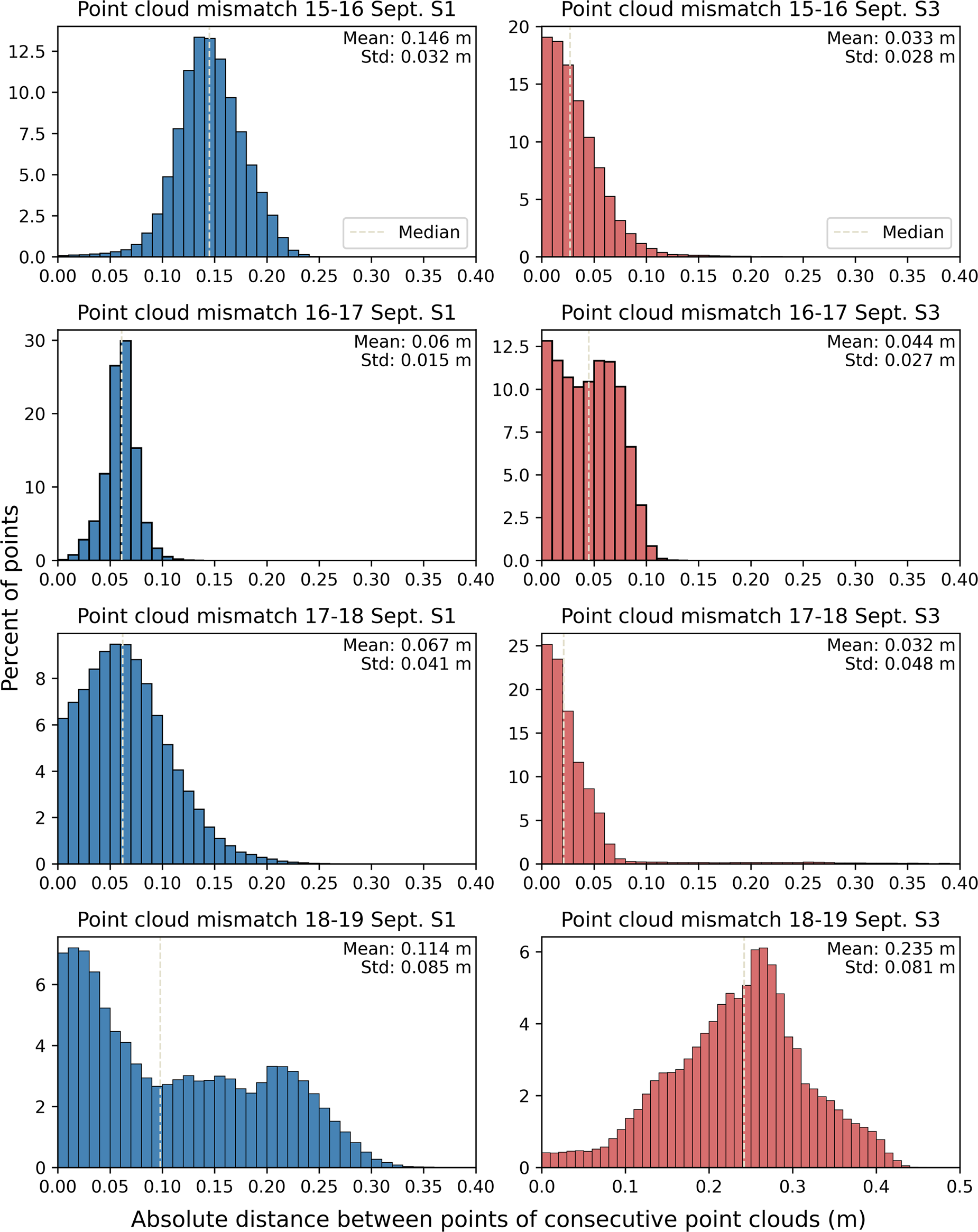
To estimate the uncertainty of the calving detection and, consequently, the volume estimation, we calculate the misfit of consecutive point clouds in areas where no calving was observed throughout the measurement period (15–18 September 2022). For this analysis, we chose two areas, one close to the GCPs in sector I and one further away from the GCPs in sector III of the calving front (indicated in Fig. 4). For both areas and each point cloud pair, we show the distribution of absolute point distances of all points within the non-calving areas and calculate the arithmetic mean and standard deviation.
3.6 Quantification of calved volumes
For the quantification of ice volumes calved from Sálajiegna's front, we apply, to our knowledge for the first time in a glaciological setting, a surface reconstruction method that has previously been successfully used in quantifying rockfall volumes (van Veen and others, Reference van Veen, Hutchinson, Kromer, Lato and Edwards2017; Bonneau and others, Reference Bonneau, DiFrancesco and Hutchinson2019; DiFrancesco and others, Reference DiFrancesco, Bonneau and Hutchinson2020, Reference DiFrancesco, Bonneau and Hutchinson2021; Walton and Weidner, Reference Walton and Weidner2023). Each point cloud associated with an individual detected calving event (Fig. 4e) is first imported to MATLAB. There, the surface reconstruction (and associated subsequent straightforward volume calculation, attained by filling the domain enclosed by the surface with a finite number of tetrahedrons of known volume) is performed, based on the alpha shape algorithm introduced by Edelsbrunner and Mücke (Reference Edelsbrunner and Mücke1994). From the point cloud, this algorithm produces a triangle-based surface mesh with elements controlled by a parameter α that is allowed to range between α = 0 (in which case the triangle-shaped mesh element is just a point) and α = ∞ (in which case the convex hull of the point cloud is rendered) (Edelsbrunner and others, Reference Edelsbrunner, Kirkpatrick and Seidel1983). To achieve the best possible volume estimation (surface reconstruction), an optimal value of α needs to be determined that neither overgeneralises the shape of the calved volume (overestimating the volume) nor fits it too tightly (underestimating the volume). The optimal α value is identified visually by plotting all possible α-values that generate a unique shape (surface and associated volume) against their volumes. With increasing α, volumes will increase towards an asymptotic limit. The optimal α is the smallest α after the volume change rate suddenly decreases (Carrea and others, Reference Carrea, Abellan, Derron, Gauvin and Jaboyedoff2021).
For the UAV-based surveys, calved volumes were quantified using a DoD method. We do so to compare the surface reconstruction results to a better-established method previously successfully applied to calving events (e.g. Jouvet and others, Reference Jouvet2019). For this, two consecutive DEMs were subtracted in Esri ArcPro, after which single calving events were outlined manually based on the UAV-derived hillshades and orthoimages. To retrieve the final calving volume, all pixels within each outlined calving zone were summed.
3.7 Ice surface velocities in the wider Sálajiegna terminus area
High-resolution ice flow velocities were calculated by template matching using the image georectification and feature tracking toolbox (ImGraft) (Messerli and Grinsted, Reference Messerli and Grinsted2015) in MATLAB. For the template matching, we use orthoimages with a spatial resolution of 10 cm from UAV surveys on 15 and 19 September 2022, a grid spacing of 2 m, a template size of 40 pixels (4 m), and a search window size of 120 pixels (12 m). The template matching process results in absolute displacement values of template points between two surveys, hence velocity. We recalculate the measured movement within four days to a daily average for better interpretation.
4. Results
4.1 USV-based photogrammetry and terminus morphology
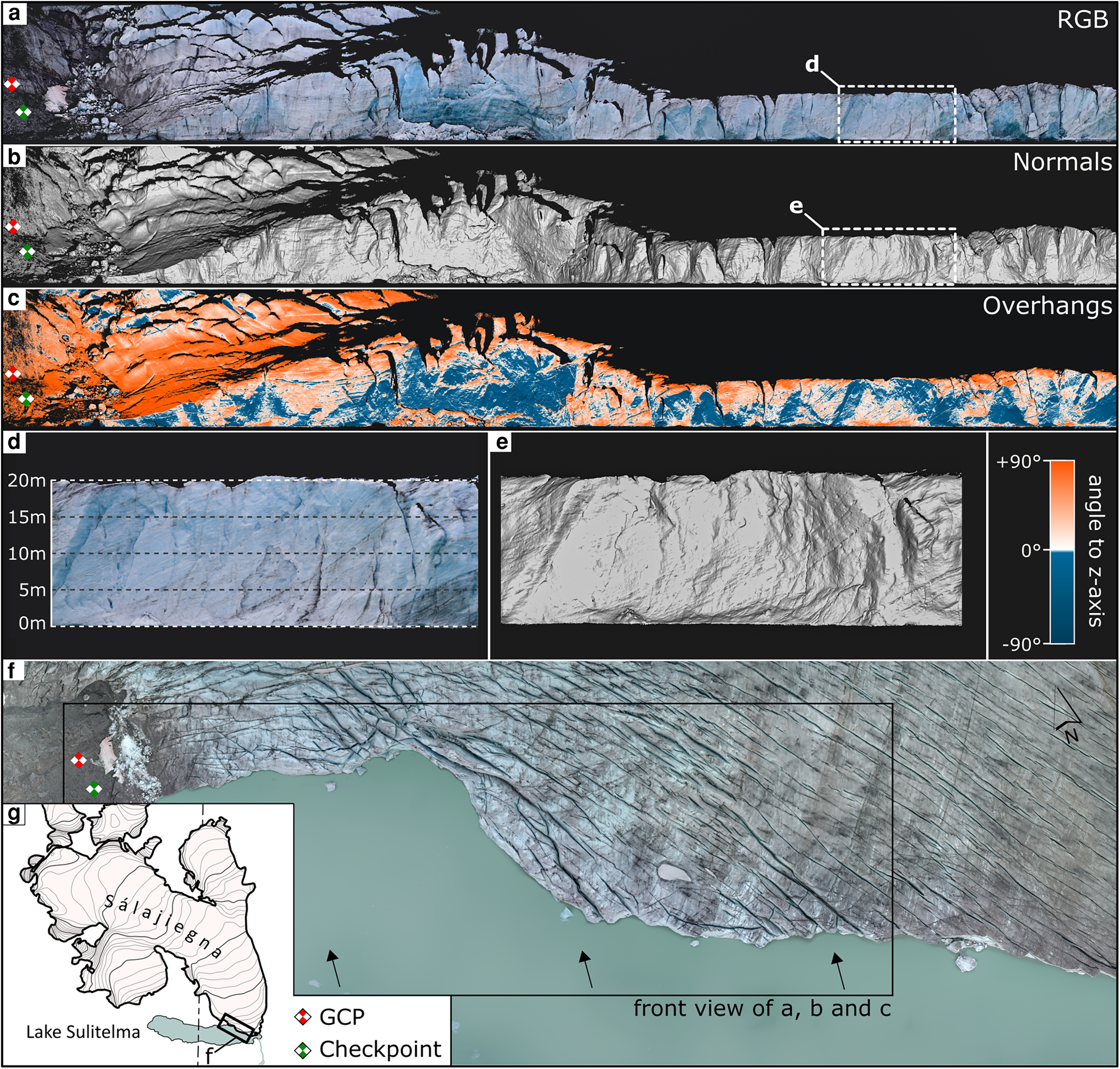
Four USV-photogrammetric surveys were successfully completed, providing high-resolution point clouds of the glacier front for four consecutive days. Results from the survey conducted on 16 September 2022 are exemplified in Figure 5. Panels a and b display the calving front (western part) using RGB values and point normals, rendering a shaded relief, respectively. In panel c, the angle between the surface normal and the z-axis is plotted, visualising the location of glacier terminus overhangs (characterised by negative such angles). Panels d and e provide a close-up of the calving front, revealing local surface structure, showing cracks in the ice, and indicating a calving front height of 20 m in this part of the glacier. A maximum calving front height of 38 m in the western part was measured in the USV-based point clouds. Contrary to the UAV surveys, only one checkpoint could be established to assess the georeferencing error, which resulted in an error of 0.07 m. However, we additionally provide the misfit between two consecutive point clouds (after ICP correction). Details of the assessment are found in Appendix C, Figure 12. We find a mean misfit of point clouds of 0.096 m in sector I and 0.086 m in sector III of the calving front. We identify the largest misfit between the last point cloud pair (18–19 September) with 0.114 m in sector I and 0.235 m in sector III.
Sálajiegna's calving front as captured by the USV on 16 September 2022. (a) Rendered from a 3D point cloud with RGB colour values. (b) Calculated normals to the local surface model of the point cloud, hillshading the front so that surface structures become apparent. (c) Identification of overhanging parts of the glacier front (blue), based on the angle between surface normals and the z-axis. (d) and (e) Close-up details of the calving front, showing the front height, surface structure, and cracks. (f) and (g) The location of the above-shown photogrammetric products in relation to the glacier.
4.2 UAV-based photogrammetry of the wider Sálajiegna terminus region
Six UAV-photogrammetric surveys, conducted between 29 July and 19 September 2022, rendered six orthomosaics and six DEMs over Sálajiegna's calving front and the glacier's wider terminus area. These were used to calculate ice flow velocities and to assess mass loss, and also serve as background images in Figures 6, 7, 8. Uncertainty of the photogrammetric products was assessed by GNSS-measured points and resulted in a mean checkpoint error of 0.06 m for the UAV surveys. Additionally, vertical accuracy was assessed over bedrock areas, and the vertical mean per pixel standard deviation from the mean elevation resulted in an error of σ z = ±0.07 m (~2 times the GSD). It is noted that the vertical error is relatively evenly distributed but also that it is largest in steep areas. Horizontal accuracy is based on displacement fields of assumed static bedrock areas and resulted in an error of σ xy = ±0.10 m (~3 GSD).
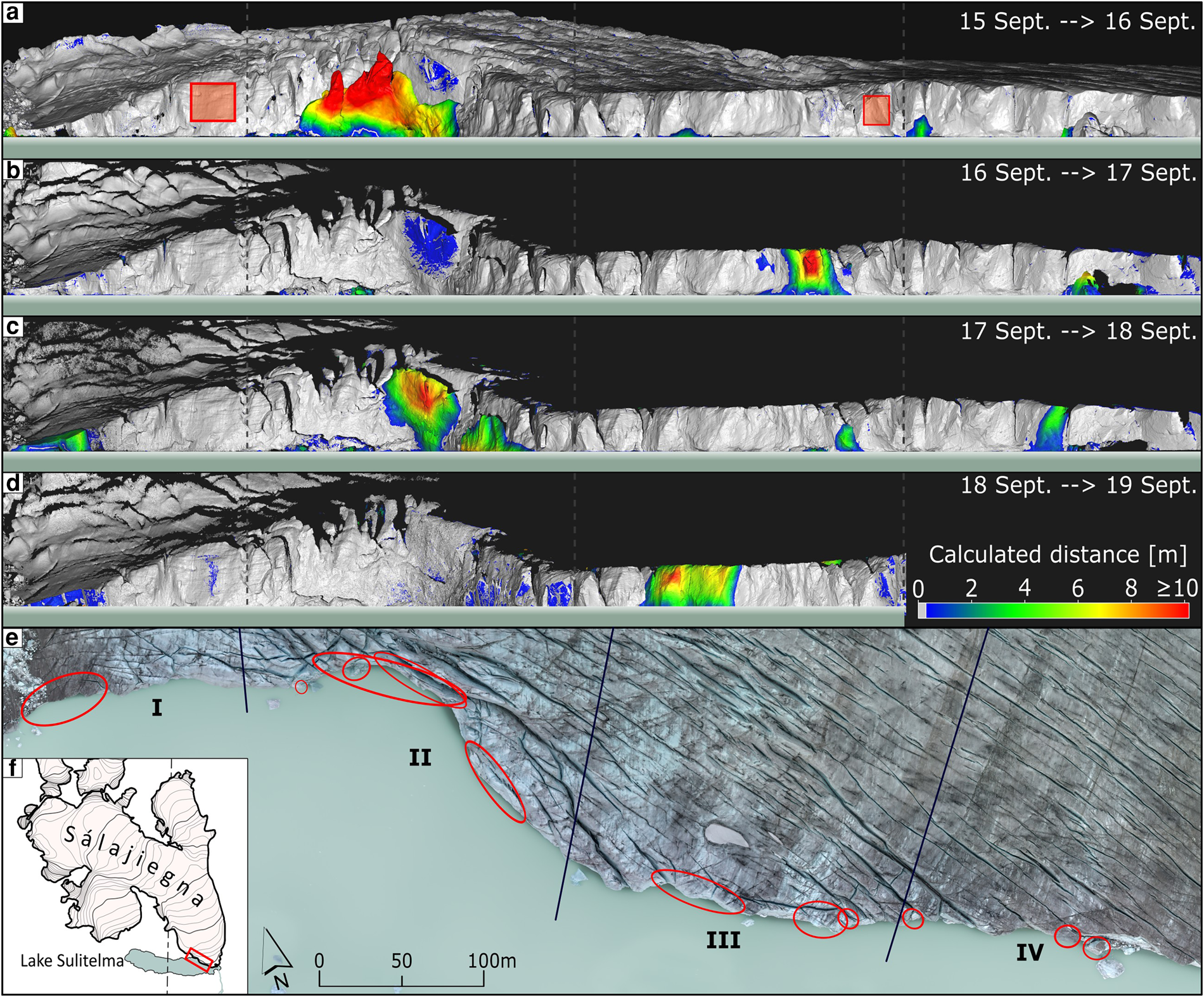
Calving detection using the M3C2 distance calculation. Panels (a) to (d) show detected calving events between consecutive surveys. Panels (e) and (f) show the location of the detection results along the glacier front, which, for reasons of easier characterisation of calving events, has been partitioned into sectors I, II, III and IV as indicated by the dashed (in panel e solid) lines. Red rectangles in (a) indicate the non-calving areas used for assessment of point cloud misfit. Image in (e) from 16 September 2022.
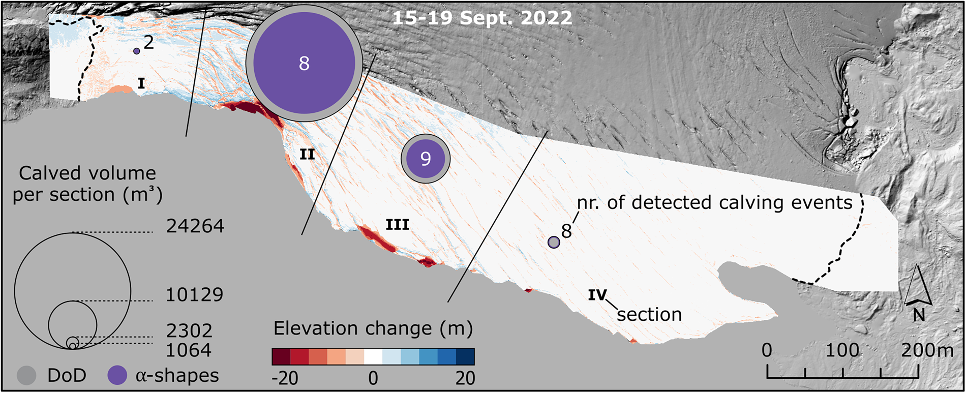
Calving characteristics between 15 and 19 September 2022 are represented by circles of various size and colour fillings for each sector (I–IV). Note that volumes given in the legend correspond to the bigger volume estimate (either DoD or alpha-shape, Table 1). Elevation change is calculated from UAV-derived DEMs (on 15 and 19 September 2022). The Background hillshade.
Salajiegna's glacier front dynamics. (a) Ice surface velocities between 15 and 19 September 2022 and USV-derived lake bathymetry. (b) Elevation change and terminus retreat between 29 July and 15 September 2022 based on UAV-derived DEMs. (c) Collapes feature seen on orthoimage from UAV survey (16 September 2022). Background in (a) and (b): DEM from UAV survey on 29 July 2022.

Detected calving events, their timing, location, estimated volume, and style
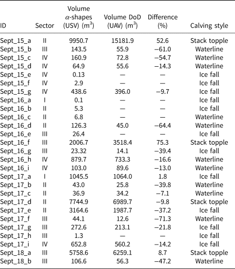
“ID” in column 1 specifies the date of the reference survey (the first of two consecutive surveys), and includes a letter counter for individual calving events. Sector (column 2) refers to the partitioning of the glacier front, as in Fig. 6. Difference (in percentage, column 5) is based on subtracting the α-shape volume (column 3) from the DoD volume (column 4) and dividing by the α-shape volume. Column five contains a classification of calving style according to How and others (Reference How2019) and Holmes and others (Reference Holmes2021). The total volume of all calving events is 32810.7 m3 for the α-shape surface reconstruction approach and 37366.2 m3 for the DoD approach - a difference of 13.8 %
4.3 Short-term calving dynamics at Sálajiegna glacier
Between 15 and 19 September 2022, a total of 27 calving events could be detected along Sálajiegna's front with volume estimates ranging from 0.1 m3 to 9950.7 m3 (Table 1). Most events were in the range of 100 to 1000 m3. The cumulative calved ice volume, calculated by surface reconstruction, is 32810.7 m3. For comparison, volumes were also estimated by a DoD approach, rendering a range of 12.6 to 15181.9 m3, with most calving events being in the range of 10 to 100 m3. The cumulative calved ice volume, calculated by DoD, is 37366.2 m3 (Table 1). The calved volumes are discussed further below.
In Figure 6, the calving source areas are indicated with a blue-green-yellow-red colour spectrum corresponding to the calculated local distance between point clouds. Areas of no change (<0.2 m) are displayed in grey. Note that the first calving detection (Fig. 6a) relies on a comparison of a USV survey conducted on 16 September 2022, to a UAV survey performed on 15 September 2022, because no USV survey could be conducted on that day. Some areas (e.g. Fig. 6b, sector II, blue area) indicate a calving event, however, a closer inspection reveals that only the beginning of a calving event is seen, e.g when an overhanging sérac tilted forward one day and collapsed the next day. Once detected, the 3D points corresponding to a calving event could be used for a surface reconstruction based volume estimation (Table 1).
An alternative representation of the calved volumes is presented in Figure 7, showing that most of the calving events were detected in sector III (nine events) and that sectors II and IV are almost as active with regard to calving (eight events each). In sector I, only two calving events were detected. In terms of calved volume, more than 75 % could be attributed to sector II, with losses clearly dominated by stack topple calvings (78 %), and complemented by ice fall (17 %) and waterline (5 %) calvings.
Between 15 and 19 September 2022, the glacier front retreated as much as 17.5 m in areas with active calving. The biggest retreat was measured in sector II, however, sector III also retreated up to 15.3 m. In the same time period the glacier front, where no calving took place, advanced about 0.5 m in the west while being close to static in the east. During the USV surveys, lakefloor bathymetry along the calving front was mapped, and is displayed in Figure 8a. Maximum depths of 23 m were recorded along the front, implying that - given the height of the calving front above water - Sálajiegna's terminus is grounded. In parts of sectors III and IV, the terminus appears to be located on a retrograde slope, i.e., lakefloor deepening towards the present glacier front position. Locally, exceptions are observed, such as along the eastern edge of sector II and centrally in sector III, where very shallow depths have been recorded by the USV.
4.4 Short-term ice surface velocities
Glacier surface velocities in Sálajiegna's terminus regions were calculated between 15 and 19 September 2022, based on the UAV-derived orthomosaics, and are shown in Figure 8a. Generally, flow velocities are highest in the west (sectors I, II and parts of sector III), and lowest in the east (parts of sector III, and in sector IV). Even though the glacier is laterally in contact with bedrock in its western terminus region, flow velocities average to 12 cm d−1 in sector I. The maximum ice surface velocity of 22 cm d−1 is reached in sector II (averaging at 14 cm d−1). Contrarily, in sector IV, flow velocities are lowest, averaging at 3 cm d−1. Sector III represents a transition zone between slow flow in the east and fast flow in the west and averages at 10 cm d−1. Between July and September, flow velocities could not be calculated, as the deformation of the ice and the change of the front positions were too large.
4.5 Seasonal frontal retreat, surface elevation changes, and mass loss at Sálajiegna glacier
To assess the glacier front dynamics during the calving season of 2022, UAV-derived aerial images and digital elevation models from 29 July and 15 September 2022 were compared. A maximum terminus position retreat of 56 m was revealed by outlining the glacier fronts (Fig. 8b). Note that the northwest-southeast oriented part of the glacier front (sectors I-III, and parts of sector IV) shows high retreat, while the east-west oriented part in sector IV shows almost no change over the calving season 2022.
Seasonal surface elevation changes in the immediate calving region of Sálajiegna, derived from a DoD approach using DEMs acquired on 29 July and 15 September 2022, are shown in Figure 8b. Given the area over which the elevation change occurs, a volume loss (above the waterline only) of 330211 m3 is derived for the immediate calving area. In the wider terminus region upstream of the calving region (coloured area in Fig. 8b), a mean surface lowering of 2.6 m was calculated, translating to a thinning rate of 5.4 cm d−1 during the 48-day period. This corresponds to a volume loss of 582462 m3 over the given area.
From adding the volume losses in the immediate calving region to those in the wider terminus region and the volume of ice calved during 15 to 19 September 2022 (Table 1) it is suggested that a minimum of 945484 m3 (surface reconstruction based on α shapes) to 950039 m3 (DoD) of ice was lost from 29 July to 19 September 2022. Note that this is a lower bound for the total volume loss because only ice loss above the waterline is accounted for and ice flow is neglected. Assuming an ice flow velocity similar to the velocity as it was measured in September, the glacier could have advanced several metres, resulting in even higher numbers of ice lost due to calving.
Besides calving, a specifically high mass loss occurred at Sálajiegna's terrestrial eastern margin in the form of a collapse feature with an approximate areal footprint of 5000 m2, which formed in a region with suspected high subglacial hydrological activity (In the field and on aerial images, discharge was observed to exit the glacier in that region and a few tens of metres downstream to enter the glacier again.).
5. Discussion
5.1 Uncrewed vehicles for assessing calving front dynamics
At Sálajiegna, both a UAV and a USV were used to assess short-term calving front dynamics and mass loss during the calving season 2022. We attribute both platforms with individual capabilities and limitations (Table 2), which we discuss in the following:
Capabilities and limitations of uncrewed surface and aerial vehicles
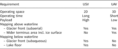
Photogrammetric surveys are best conducted not only with an along-track overlap but also with a side overlap/across-track overlap (Lopes Bento and others, Reference Lopes Bento2022). However, unlike UAVs, USVs can, in principle, only produce image sequences with an overlap in the along-track direction (along the glacier front). Nonetheless, the image matching during the SfM-MVS process posed no problem and four 3D point clouds of Sálajiegna's glacier front were created purely from the USV surveys. Despite challenges encountered during image acquisition (such as icebergs blocking either the in-between-waypoint route of the USV or the camera view from the USV to the glacier front), and despite the lack of across-track overlap, the resulting photogrammetric products show little noise. The 3D point clouds generated from the USV surveys during the SfM-MVS process show high levels of detail of the calving front with a point cloud density of 11 172 points per m3. This is approximately 15 times higher than the point cloud density of the UAV products (739 points per m3). This high resolution could be achieved mainly because the USV is capable of carrying a larger and heavier payload (in this case, a camera with a larger, higher resolution sensor and a higher-quality lens) than the UAV. Thus, we argue that a prominent capability (carrying high scientific, and also mission-enabling payload, e.g. larger batteries implying longer operating time) can compensate for a perceived limitation (restricted operating space).
A limitation of the USV, when mapping glacier parts above the waterline, concerns the camera's field of view. Operating on the 2D lake surface, the USV only captures the glacier's near-vertical terminus. Moreover, the USV's viewpoint implies that upward-facing parts of the calving front (as well as the wider terminus area) remain blind spots as they cannot be seen from a lake-level perspective. This implies that UAV surveys are needed if information regarding e.g. ice surface velocity in the wider terminus area is to be acquired because these remain elusive to USV surveys. However, we found that USV-based surveys yield better results at the contact line between ice and the lake surface than the UAV-based surveys, because point clouds from the latter show significant noise levels and hence made it difficult to identify a sharp edge defining the ice-water interface. However, with careful mission planning a UAV could be flown sideways along the glacier front, taking oblique images and achieving similar accuracy at ice-water intersection.
Depending on their size, payload and operational profile, USVs can achieve operating ranges of more than 200 km, which is significantly larger than that of most off-the-shelf UAVs, although the increased range is traded off against increased survey time. However, with additional engineering effort, UAVs are capable of similar distances (e.g. Jouvet and others Reference Jouvet2019). In the end, the operational range for both platforms comes down to financial and engineering investment.
Regardless, perhaps the most important advantages of USVs over UAVs are the extended payload options. Not only can USVs carry larger payloads (e.g. a full-frame digital camera), but their payload suite is also highly customisable, allowing, for example, the use of underwater acoustic imaging sensors for mapping seafloor and lake floor bathymetry. Ongoing developments aim at improved mapping capabilities for USVs (see Section Perspectives).
At larger glaciers, challenges associated with an ice mélange in front of the terminus could hinder the manoeuvring of the USV. This limitation can only be partially overcome through dedicated hull design and increased propeller thrust. Furthermore, the operation of UAVs (and, to some extent, USVs) can also be restricted by atmospheric conditions, particularly strong glacier winds or a low cloud base.
Solely USV-based assessments of calving behaviour are likely limited to slow-flowing glaciers, as for fast-flowing glaciers, knowledge of and compensation for flow velocities would be necessary. Furthermore, the volume estimation of full-thickness calving events based on USV data is not advisable, as only the glacier front is within the USV's field of view. Nonetheless, the deployment of USVs at larger, fast-flowing glaciers can be advocated to acquire information about glacier front properties or bathymetry.
Both USVs and UAVs are available as commercial products, even though USVs are niche products and manufactured only by a few highly-specialised companies (e.g. BlueRobotics, SeaFloor Systems, EvoLogics, Maritime Robotics), whereas UAVs have been available on the consumer electronics market for several years. The prices for entry-level UAVs are significantly lower than those of commercial USVs. It is, however, difficult to quantify the research- and development costs for a scientific prototype as was used in this study.
5.2 Calving detection
A detection of calving events at Sálajiegna's front has been accomplished by a point cloud based distance calculation (M3C2 algorithm, cf. Section Methods) with photogrammetric products obtained by the USV, which by design is a moving platform. This advances previously reported point cloud based glaciological applications that focus mainly on static-position, repeat scan, or LiDAR-acquired datasets to characterise calving glacier fronts (Pe¸tlicki and Kinnard, Reference Pętlicki and Kinnard2016; Mallalieu and others, Reference Mallalieu, Carrivick, QUINCEY, Smith and James2017; Podgórski and others, Reference Podgórski, Pe¸tlicki and Kinnard2018; Köhler and others, Reference Köhler2019).
Operating from a moving platform can, on the one hand, be considered advantageous because a USV can be manoeuvred to positions that enable views of the glacier front that may not be in the line of sight of a statically placed system. On the other hand, drifting lake ice, calved ice, and wind may make surveys from a moving platform more difficult compared to surveys carried out from static systems.
At Sálajiegna, we found the mobility of the USV in combination with the application of the M3C2 algorithm to the survey data advantageous, as it provided more detail compared to a DoD approach: 27 calvings were detected by M3C2, while only 20 were captured by DoD. This is likely attributed to the fact that with the M3C2 approach, changes in the overhanging parts of the glacier front can be detected, while this is not the case for the DoD approach. The calving detection process is fairly efficient, as it operates directly on the point clouds without the need to create secondary products like DEMs. However, as the generation of the point cloud is relatively computationally demanding, overall computational demands remain comparable between the two approaches, rendering neither one less costly than the other.
Also, irrespective of whether M3C2 or DoD are applied, it is emphasised that all detected calving events represent the change between surveys on consecutive days. Therefore, detected change does not necessarily correspond to a single calving event. Rather, a specific calving event may be of cumulative nature, namely when it is composed of several smaller consecutive calving events in essentially the same location. An example of this was observed on 15 September, when a series of at least eight calving events were noted, all taking place within approximately one hour in sector II of Sálajiegna's front (Fig. 6a).
When using the M3C2 algorithm on the USV-survey point clouds with the primary goal of detecting calving events between consecutive days, it must be recalled that glacier flow over this period also contributes to mapped frontal changes. This issue can be addressed in two ways: First, a detection limit can be set, below which any observed changes are not regarded as calving events but are attributed to glacier flow. As this detection limit must not be too large (it was set to 0.2 m here), it is suggested that such an approach is only applied to slow-flowing glaciers, and where the threshold is determined in situ to yield the best possible results. Second, the time between consecutive surveys could be reduced in order to allow for small threshold detection values, however, this might not always be practically possible in the field.
5.3 Volume estimation
Following the calving detection, calved volumes were derived from a DoD (for the UAV-based surveys) and an α-shape (for the USV-based surveys) approach, respectively.
The α-shape based approach allowed for the reconstruction of a range of different calving event sizes. The DoD approach did not detect some of the events, especially smaller and medium-sized events. This is likely attributed to the fact that the change detection in the DoD approach is in vertical (z) direction only and misses calving events beneath overhanging parts of the glacier front (Figs. 9a,b). Hence, the DoD approach could be expected to underestimate total calved volumes. However, this reasoning changes when looking at large calving events: their volume (cf. the stack topple style calvings on 15, 16, 18 September in Table 1) is overestimated in the DoD approach because it includes the often ice-free area underneath an overhang (Fig. 9c). Hence, because the large calving events are the largest contributors to the cumulative calved volume, the total calved volume is likely overestimated when the DoD method is used. The same applies for estimations of total calved volume derived by using the α-shape based approach, because the algorithm, by construction, interpolates the 3D points and generalises the actual shape of the point cloud (Edelsbrunner and Mücke, Reference Edelsbrunner and Mücke1994). However, the degree of generalisation strongly depends on the point cloud's quality: for low-quality clouds, high α values have to be chosen, leading to a stronger generalisation and, hence, overestimation of volumes. Bonneau and others (Reference Bonneau, DiFrancesco and Hutchinson2019) report an overestimation of rockfall volumes of approximately 10 % with a point distance of 10 cm (which is approximately twice the distance between points in the USV-based point clouds used for the calculation in this study). Overestimation of calved volume based on the α-shape approach is particularly obvious for the waterline and ice fall calvings (Table 1) for which the DoD volumes are smaller in all but one observed calvings (exception for ice fall calving on 17 September, in sector I). An error reducing the estimated amount of the α-shape volumes is introduced by the detection threshold, as areas below (in this case) 20 cm are not included. A quantitative error estimation of the calving events is difficult as many different error sources create a complex overall error. However, the mean point cloud misfit of less than 10 cm shows that after applying the ICP correction, the remaining georeferencing and flow velocity errors are within a reasonable range to perform the volume estimation.
DoD volume estimation errors. (a) No estimation is possible because the calving event is entirely underneath the overhang. (b) Underestimation of the actual volume due to the calving event being partly underneath the overhang. (c) Overestimation of the actual volume because the volume underneath the overhang is included.

In conclusion, both approaches seem to overestimate the total calved volume. However, because the α-shape based approach is more versatile (for high-resolution studies like here), especially with regards to detecting changes in overhanging areas and hence rendering a smaller overestimation than the DoD-based approach (in numbers: 13.8 %), it is suggested that the estimated calved volume of 32810.7 m3 (from the α-shape approach) is seen as the best possible approximation of actual volume calved above the waterline. Based on the discussion above, we argue that the high-resolution point clouds, in combination with the α-shape approach, reduce the volume estimation error for small, medium, and large calving events. Both estimates are, however, likely underestimates of total calved volume because calving from the submerged parts of the glacier front is not yet quantified and hence not included in estimates of total calved volume.
5.4 Short-term calving front dynamics at Sálajiegna glacier
During 15–19 September 2022, an average of 5.4 calving events per day were detected. Most events occurred in sector III, but the largest ice volume calved from sector II, where it amounts to 2, 10, and 20 times that of sectors III, IV, and I, respectively (Fig. 7). Most of the calved volume stems from two big calving events in sector II (Table 1). Since the observational period was not only limited in time but also the first during which Sálajiegna's calving processes were studied in detail, no conclusions can be drawn regarding how representative the observed short-term calving is with respect to the overall calving behaviour during an entire season, or how calving behaviour varies between years. Nonetheless, we note that the high calving activity in sector II coincides with higher flow velocities measured in this sector and deeper water depths compared to other sectors. Flow velocities can be the cause or effect of high calving rates as discussed by Benn and others (Reference Benn, Warren and Mottram2007). Water depth at a glacier terminus has long been empirically related to the calving rate, in the sense that the calving rate is higher for termini grounding in greater water depths than those grounding in shallower waters (Brown and othres, Reference Brown, Meier and Post1982; Pelto and Warren, Reference Pelto and Warren1991). However, proper identification of the drivers of calving at Sálajiegna is impossible based on the data presently available. With respect to calving activity, the roles of bathymetry, the thermal state of Lake Sulitelma, and climatological conditions remain to be investigated - preferably on multi-annual time scales.
5.5 Seasonal frontal retreat and mass loss at Sálajiegna glacier
Lake Sulitelma is ice-covered for most of the year, and the backstress exerted by the ice cover is likely to reduce or even suppress calving activity at Sálajiegna glacier, as observed and modelled for other glaciers (Todd and Christoffersen, Reference Todd and Christoffersen2014; Otero and others, Reference Otero2017; Barnett and others, Reference Barnett, Holmes and Kirchner2022). Satellite imagery provides approximate ice-off (fully ice free) and ice-on (full ice cover) dates at Lake Sulitelma, suggesting that the lake was ice-free from mid-July 2022 (ice-off) to the end of September 2022 (ice-on). Hence, the period between the first (29 July 2022) and last (19 September 2022) survey spans nearly the entire calving season. However, calving at Sálajiegna's terminus does not immediately start after ice-off: Both during 2022 and during previous fieldwork at the same site in 2020 (when ice-off however took place in mid-August), the onset of calving was observed to lag behind ice-off at Lake Sulitelma. However, this lag is not yet systematically quantified - this would require the use of e.g. satellite imagery to determine dates (or date ranges) for ice-off as well as the onset of calving over a longer time period and may be investigated in the future. During Lake Sulitema's ice-free period in the summer of 2022, Sálajiegna's freshwater-terminating front retreated up to 56 m in the central part of sector III.
This summer retreat is larger than average annual retreat rates from the 20th century inferred from Østrem (Reference Østrem1983) and Klingbjer and others (Reference Klingbjer, Brown and Holmlund2005), cf. also Appendix A. This is partially expected, as any potential winter advance modulating the net annual retreat to lower numbers has not been included. Also, it is noted that the comparison to earlier observed retreat rates is very rough, because the former were calculated along transects which do not include the location where the largest retreat during the summer 2022 was observed. Retreat rates are not spatio-temporally homogeneous: the eastern part of sector IV appears rather static since 2020, in contrast to the rapid retreat observed in sector III (Fig. 8).
Besides frontal retreat, Sálajiegna glacier has shown an average thinning amounting to 2.6 m or 5.4 cm d−1 in the wider terminus region (cf. Fig. 8b, coloured area upstream of glacier front position on 15 September), during the summer of 2022. This is in a similar magnitude as the annual average thinning of 2.3 m for the period 1950–1992, based on contemporary and previously published maps (Østrem, Reference Østrem1983; Klingbjer and others, Reference Klingbjer, Brown and Holmlund2005). While these comparisons provide a glimpse of Sálajiegna's overall dynamic evolution over the past decades, they do not reveal much detail as previously available data is temporally sparse (mainly in the form of maps from 1950, 1957, 1971, 1983 and 1992), non-digital with unspecified accuracy, and coarser spatial resolution. While the continuing overall frontal retreat at Sálajiegna is undisputed (Østrem, Reference Østrem1983; Klingbjer and others, Reference Klingbjer, Brown and Holmlund2005; Hill, Reference Hill2021), investigating rates of retreat and mass loss on timescales that allow for attribution of drivers of change, and for assessment of current and future mass loss rates, remains an ongoing challenge.
6. Perspectives
In this study, the main purpose of the USV was to investigate the feasibility of a USV-based calving detection with simultaneous echosounder-based mapping of the lake floor bathymetry, taking advantage of the payload capacity of the USV. However, given the financial and technical resources, USVs can be equipped to perform a variety of glaciological and oceanographic measurements.
An example of this development is the successor of the USV used in this study, called Kuninganna, which was also developed at the KTH Royal Institute of Technology in Stockholm. This USV has been equipped with a multibeam echosounder instead of a single beam echosounder, providing high-resolution bathymetry products, which, in combination with bedrock data, are crucial for glacier modelling. Furthermore, the multibeam sonar can be used to scan the submarine part of the glacier front.
Additionally, USVs are capable of collecting in-situ oceanographic data (e.g. with CTD winches and turbidity sensors) to provide insights into meltwater plumes and submarine melt, which are especially valuable for glacier models regarding ice-ocean interactions. Other additional sensors can, for example, include LiDARs and towed acoustic arrays.
One could envision a future in which higher grades of autonomy (both in terms of energy capacity and intelligent behaviour) will enable the long-term presence of USVs at calving glacier fronts and allow for continuous measurements and mapping. However, such a vision will face technological and operational challenges, as discussed (see Section Discussion).
7. Conclusions
Results were presented from combined USV- and UAV-based photogrammetric surveys conducted at Sálajiegna, northern Sweden. The novelty of the presented approach, on one hand, lies in integrating a photogrammetric payload suite into the USV and, on the other hand, in conducting a point cloud based calving detection and surface-reconstruction based volume quantification of ice lost due to calving. Based on an initial survey in July 2022, at the beginning of Sálajiegna's calving season, and four consecutive surveys in September 2022, we find that:
USVs are well-suited to perform photogrammetric surveys of calving glacier fronts, while the ability to perform a change detection is limited to slow-flowing glaciers. Because of their ability to collect data above and below the water surface and because they can carry high scientific payloads, USVs are versatile platforms for glaciological research.
Calving events at Sálajiegna glacier were successfully detected using the M3C2 algorithm operating directly on the high-resolution point clouds from the USV surveys. This approach is a promising alternative to DEM of Difference approaches.
The short measurement period and the lack of previous research at this glacier limit the interpretation of glaciological findings. Nonetheless, we find a thinning rate in the terminus region of 5.4 cm d−1 and a maximum terminus retreat of 56 m during the summer of 2022 and identify a region of higher flow velocities and higher calving activity during the 5-day period in September.
Acknowledgements
We would like to thank Ann-Kathrin Wild and Daniel Wilhelmsson for their support in the field and Niklas Rolleberg, KTH Royal Institute of Technology, for his technical support. Tovo Spiral, Arctic Guides Abisko, is thanked for providing invaluable logistical support in connection with the field work period at Sálajiegna in September 2022. Funding from The Göran Gustafsson Foundation (awarded to Kirchner) and the research unit Geomorphology and Glaciology at the Department of Physical Geography at Stockholm University (awarded to Vacek) is gratefully acknowledged.
Appendix A
This Appendix contains Figure 10 and Table 3, and provides additional information concerning the recent evolution of Lake Sulitelma, and Sálajiegna's calving front dynamics.
Outlines of Sálajiegna's eastern and western terminus in the years 1950, 1957, 1971, 1983 Østrem (Reference Østrem1983), 1992, 2008 and 2022, based on maps by Østrem (Reference Østrem1983); Klingbjer and others (Reference Klingbjer, Brown and Holmlund2005) and, for 2008 and 2022, on aerial images from the Land Survey of Sweden (Lantmäteriet). Changes on frontal geometry over time induced changes in the extent of Lake Sulitelma, and its drainage pathways. Background image is from a 1 m Digital Elevation Model by Lantmäteriet, used to identify moraines suggesting Sálajiegna's maximal extent at the peak of the Little Ice Age (LIA), occurring ca. 1910 in this region. Frontal retreat is exemplified along transects A and B in Table 3.
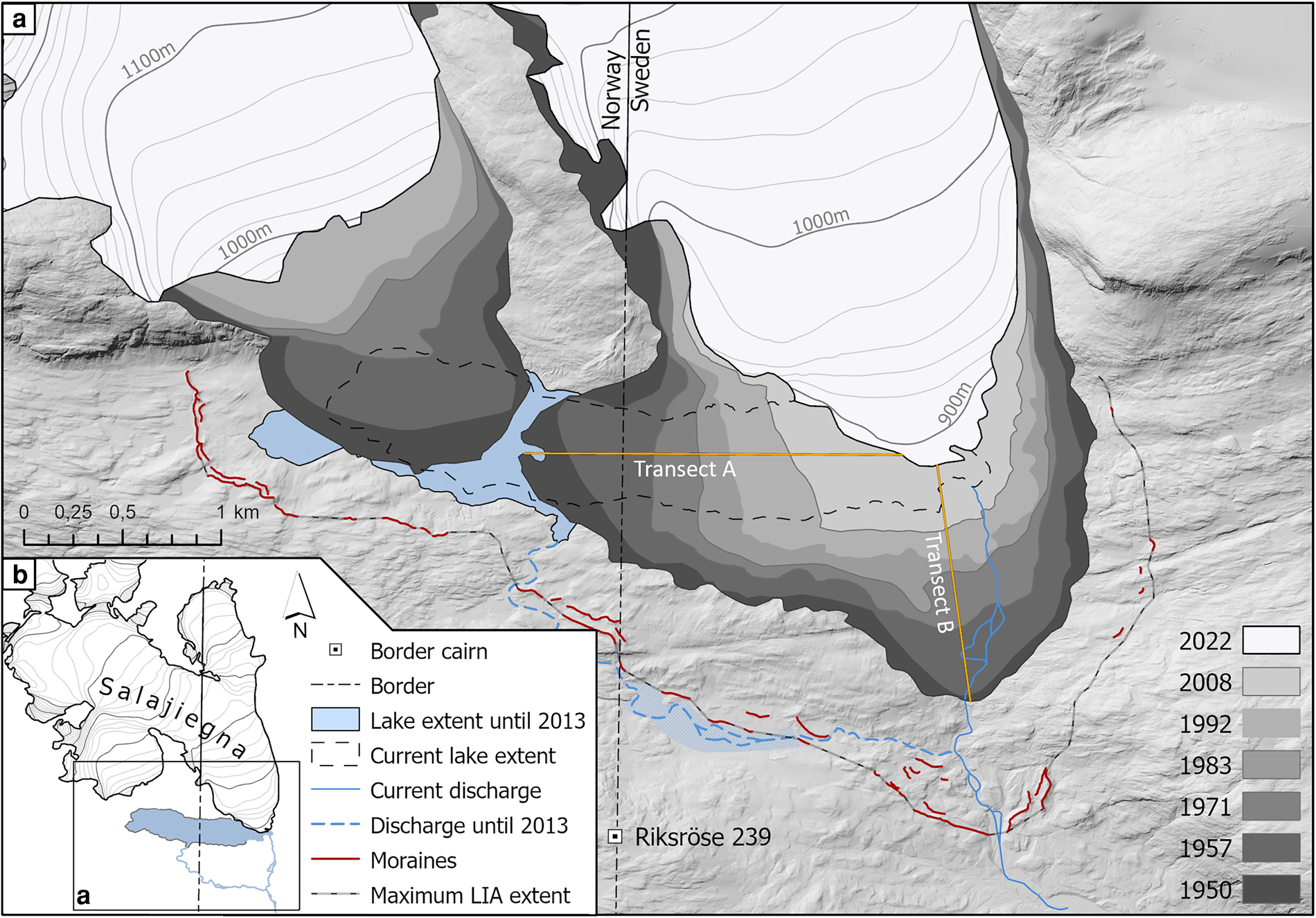
Retreat rates along the transects shown in Figure 10, based on maps by Østrem (Reference Østrem1983); Klingbjer and others (Reference Klingbjer, Brown and Holmlund2005) and aerial images by Läteriet (2008 and 2022)
Appendix B
This Appendix contains Table 4 and provides a summary of USV and UAV survey details.
Summary of USV and UAV surveys as well as characteristics of their resulting point clouds

Appendix C
This Appendix contains Figure 11 to showcase the visual verification of a calving event with a complex outline and Figure 12 showing the point cloud misfit histograms of each point cloud pair and for two non-calving areas as indicated in Figure 6.
Visual verification of calving event Sept_16_e and parts of Sept_16_f (bottom) (a) Image before calving event on 16 September (b) Image after calving event on 17 September (c) Detection result.
Statistics showing the misfit between consecutive point clouds as the absolute distance between points of non-calving areas indicated in Figure 6. Blue corresponds to the non-calving area in sector I, and red corresponds to the non-calving area in sector II. The first row shows distances between the first and second surveys, the second row between the second and third surveys, and so forth. Note the different x-axis for the bottom right plot, which shows higher distances than all other areas.


 Open access