





1 Introduction
The focus of our research is the spectrum of discrete multidimensional quasi-periodic Schrödinger operators on
$\ell ^2({\mathbb Z}^d)$
 , given by

where
$|\boldsymbol {m}-\boldsymbol {n}|=\sum _{i=1}^d |m_i-n_i|$
 , and
$\lambda \in {\mathbb R}$
, and
$\lambda \in {\mathbb R}$
 is the coupling constant. Here, we assume that the potential
$V: {\mathbb T}^d \rightarrow {\mathbb R}$
is the coupling constant. Here, we assume that the potential
$V: {\mathbb T}^d \rightarrow {\mathbb R}$
 is continuous, and
$\vec {\alpha }=(\alpha _1,\cdots ,\alpha _d)$
is continuous, and
$\vec {\alpha }=(\alpha _1,\cdots ,\alpha _d)$
 with
$(1,\vec {\alpha })$
with
$(1,\vec {\alpha })$
 rationally independent is the frequency, and we denote
$\boldsymbol {n} \vec { \alpha }=(n_1\alpha _1,\cdots ,n_d\alpha _d).$
rationally independent is the frequency, and we denote
$\boldsymbol {n} \vec { \alpha }=(n_1\alpha _1,\cdots ,n_d\alpha _d).$
 Our main interest lies in determining whether (1.1) possesses Cantor spectrum.
1.1 Cantor spectrum for 1D Schrödinger operators
When
$ d=1 $
 , the most prominent example of the operator defined in (1.1) with a Cantor spectrum is the Almost Mathieu Operator (AMO)
$H_{\lambda ,\alpha ,\theta }$
, the most prominent example of the operator defined in (1.1) with a Cantor spectrum is the Almost Mathieu Operator (AMO)
$H_{\lambda ,\alpha ,\theta }$
 , defined on
$\ell ^2(\mathbb {Z})$
, defined on
$\ell ^2(\mathbb {Z})$
 as follows:

The AMO was originally introduced by Peierls [Reference Peierls62] as a model for an electron on a two-dimensional lattice subjected to a homogeneous magnetic field [Reference Harper40, Reference Rauh65]. The famous “Ten Martini Problem” [Reference Kac52, Reference Simon66] asserts that
$ H_{\lambda ,\alpha ,\theta } $
 has a Cantor spectrum for any
$ \lambda \neq 0 $
has a Cantor spectrum for any
$ \lambda \neq 0 $
 and
$ \alpha \in \mathbb {R} \setminus \mathbb {Q} $
and
$ \alpha \in \mathbb {R} \setminus \mathbb {Q} $
 . This was ultimately proved by Avila and Jitomirskaya [Reference Avila and Jitomirskaya8], building on earlier contributions [Reference Avila and Krikorian10, Reference Bellissard and Simon16, Reference Choi, Elliott and Yui21, Reference Helffer and Sjöstrand45, Reference Last57, Reference Puig63]. Building on methods developed for the quantitative aspects of Avila’s global theory [Reference Avila5, Reference Ge, Jitomirskaya, You and Zhou33], it was recently shown that any Type-1 operator with a triorthogonal potential has Cantor spectrum [Reference Ge, Jitomirskaya and You31, Reference Ge, Jitomirskaya and You32]. Meanwhile, Argentieri and Avila [Reference Argentieri and Avila3] proved that there exist analytic perturbations of subcritical AMO that exhibit interval spectrum. For the critical almost Mathieu operator, the “Dry Ten Martini Problem”—whether all spectral gaps are open—remains open [Reference Avila and Jitomirskaya8, Reference Avila, You and Zhou12, Reference Kac52, Reference Simon66]. A recent result by Li-Xu-Zhou [Reference Li, Xu and Zhou59] shows that any Type-1 operator with a supercritical triorthogonal potential has all gaps open, thereby partially confirming the conjecture in [Reference Ge, Jitomirskaya and You31, Reference You76].
For more general potentials
$ V $
 , Simon [Reference Simon66] conjectured that the operator defined in (1.1) generically exhibits a Cantor spectrum. The first foundational result establishing the existence of a Cantor spectrum was obtained by Sinai [Reference Sinai68] for large
$C^2$
, Simon [Reference Simon66] conjectured that the operator defined in (1.1) generically exhibits a Cantor spectrum. The first foundational result establishing the existence of a Cantor spectrum was obtained by Sinai [Reference Sinai68] for large
$C^2$
 cosine-type potentials; this result was later reproved using different methods in [Reference Forman and VandenBoom29, Reference Wang and Zhang74]. Eliasson [Reference Eliasson25] proved that for any fixed Diophantine frequency
$ \alpha \in \mathbb {R} \backslash \mathbb {Q} $
cosine-type potentials; this result was later reproved using different methods in [Reference Forman and VandenBoom29, Reference Wang and Zhang74]. Eliasson [Reference Eliasson25] proved that for any fixed Diophantine frequency
$ \alpha \in \mathbb {R} \backslash \mathbb {Q} $
 and for generic small analytic potentials, (1.1) possesses a Cantor spectrum. This result was subsequently extended to the entire subcritical regime and any irrational
$ \alpha \in \mathbb {R} \backslash \mathbb {Q} $
and for generic small analytic potentials, (1.1) possesses a Cantor spectrum. This result was subsequently extended to the entire subcritical regime and any irrational
$ \alpha \in \mathbb {R} \backslash \mathbb {Q} $
 [Reference Li and Zhou60, Reference Puig64], via global-to-local reduction [Reference Avila4, Reference Avila6, Reference Avila and Jitomirskaya9, Reference Ge30, Reference Han and Schlag39]. Goldstein and Schlag [Reference Goldstein and Schlag35] established that for generic
$ \alpha \in \mathbb {R} \setminus \mathbb {Q} $
[Reference Li and Zhou60, Reference Puig64], via global-to-local reduction [Reference Avila4, Reference Avila6, Reference Avila and Jitomirskaya9, Reference Ge30, Reference Han and Schlag39]. Goldstein and Schlag [Reference Goldstein and Schlag35] established that for generic
$ \alpha \in \mathbb {R} \setminus \mathbb {Q} $
 in the region of positive Lyapunov exponents, the spectrum forms a Cantor set. Avila-Bochi-Damanik [Reference Avila, Bochi and Damanik7] showed that for any fixed
$ \alpha \in \mathbb {R} \setminus \mathbb {Q} $
in the region of positive Lyapunov exponents, the spectrum forms a Cantor set. Avila-Bochi-Damanik [Reference Avila, Bochi and Damanik7] showed that for any fixed
$ \alpha \in \mathbb {R} \setminus \mathbb {Q} $
 and any generic
$ V \in C^0(\mathbb {T},\mathbb {R}) $
and any generic
$ V \in C^0(\mathbb {T},\mathbb {R}) $
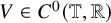 in the
$ C^0 $
in the
$ C^0 $
 -topology, the spectrum is also a Cantor set [Reference Avila, Bochi and Damanik7]. In the
$ C^k $
-topology, the spectrum is also a Cantor set [Reference Avila, Bochi and Damanik7]. In the
$ C^k $
 -topology (for
$ 1 \leq k \leq \infty $
-topology (for
$ 1 \leq k \leq \infty $
 or even in the analytic category), it has been proven that for generic
$ \alpha \in \mathbb {R} \setminus \mathbb {Q} $
or even in the analytic category), it has been proven that for generic
$ \alpha \in \mathbb {R} \setminus \mathbb {Q} $
 and generic
$ V \in C^k(\mathbb {T},\mathbb {R}) $
and generic
$ V \in C^k(\mathbb {T},\mathbb {R}) $
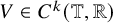 , the spectrum of (1.1) is a Cantor set. For an outline of the proof, we refer to footnote 1 in [Reference Wang, Zhou and Jäger73].
1.2 Cantor spectrum for multidimensional Schrödinger operators
Historically, it was widely anticipated that the Cantor spectrum is predominantly a one-dimensional phenomenon, rarely appearing when
$d \ge 2$
 . A related conjecture, known as the Bethe-Sommerfeld conjecture, posits that for
$ d \geq 2 $
. A related conjecture, known as the Bethe-Sommerfeld conjecture, posits that for
$ d \geq 2 $
 and any periodic function
$ V: \mathbb {R}^d \rightarrow \mathbb {R} $
and any periodic function
$ V: \mathbb {R}^d \rightarrow \mathbb {R} $
 , the spectrum of the continuous Schrödinger operator
$ -\Delta + V $
, the spectrum of the continuous Schrödinger operator
$ -\Delta + V $
 contains only finitely many gaps; that is, there are no gaps at high energy levels. This conjecture has received extensive studies over the years and was proved by Parnovski [Reference Parnovski61]. For a more detailed discussion, please refer to [Reference Kuchment56, Reference Parnovski61] and their references. Additionally, the discrete version of the Bethe-Sommerfeld conjecture has also been resolved recently [Reference Embree and Fillman26, Reference Han and Jitomirskaya38]. More recently, the resolution of the Bethe-Sommerfeld conjecture has been extended to quasiperiodic (not necessarily separable) multidimensional continuous Schrödinger operators for almost all frequencies [Reference Karpeshina, Parnovski and Shterenberg53, Reference Karpeshina and Shterenberg54].
In high-energy regimes, continuous Schrödinger operators can be treated as perturbations of the free Laplacian. Thus, in the discrete framework, it is plausible to expect that when
$ \lambda $
 is small, the spectrum of (1.1) forms an interval. This was recently proved by Takase [Reference Takase70] under the assumption that
$ V(\vec \theta ) $
is small, the spectrum of (1.1) forms an interval. This was recently proved by Takase [Reference Takase70] under the assumption that
$ V(\vec \theta ) $
 is separable (i.e.,
$ V(\vec \theta ) = V_1(\theta _1) + \cdots + V_d(\theta _d) $
is separable (i.e.,
$ V(\vec \theta ) = V_1(\theta _1) + \cdots + V_d(\theta _d) $
 ). These findings elucidate the behavior under conditions of small potential.
However, if
$ \lambda $
 is large (or if the potential is large), one would still expect that the spectrum contains an interval. The first result concerning the interval spectrum was obtained by Chulaevsky and Sinai [Reference Chulaevsky and Sinai20], later reinforced by Goldstein-Schlag-Voda [Reference Goldstein, Schlag and Voda36], who constructed a class of real-analytic functions
$ W $
is large (or if the potential is large), one would still expect that the spectrum contains an interval. The first result concerning the interval spectrum was obtained by Chulaevsky and Sinai [Reference Chulaevsky and Sinai20], later reinforced by Goldstein-Schlag-Voda [Reference Goldstein, Schlag and Voda36], who constructed a class of real-analytic functions
$ W $
 on
$ \mathbb {T}^d $
on
$ \mathbb {T}^d $
 (considered to represent a generic condition) in which, if the frequency is Diophantine and
$ \lambda $
(considered to represent a generic condition) in which, if the frequency is Diophantine and
$ \lambda $
 is sufficiently large, the spectrum of the one-dimensional operator

comprises a single interval. This indicates that in high-dimensional cases, if
$ V(\vec \theta ) $
 is degenerate or separable and
$ \lambda $
is degenerate or separable and
$ \lambda $
 is large, then the spectrum of (1.1) is likely an interval.
Based on these discussions, one might conclude that the Cantor spectrum is predominantly a one-dimensional phenomenon. However, Damanik-Fillman-Gorodetski [Reference Damanik, Fillman and Gorodetski24] constructed a class of multidimensional limit-periodic Schrödinger operators whose spectrum is a Cantor set, spurring interest in identifying a quasiperiodic example. This task is not trivial; the spectral behavior of limit-periodic Schrödinger operators diverges significantly from that of quasiperiodic operators [Reference Damanik and Fillman23], making the direct application of [Reference Damanik, Fillman and Gorodetski24]’s methods to quasiperiodic settings challenging. Nonetheless, through Aubry duality [Reference Aubry and André2] and Eliasson’s results [Reference Eliasson25], one can readily construct the long-range operator

which possesses a Cantor spectrum when
$ V_{\boldsymbol {k}} $
 decays exponentially fast. However, the challenge remains in the Schrödinger case. Indeed, as expressed by Damanik, Fillman, and Gorodetski [Reference Damanik, Fillman and Gorodetski24]:
“It would be interesting to construct examples of this type having zero-measure Cantor spectrum in which
$ L $
 is the
$ d $
is the
$ d $
 -dimensional discrete Laplacian and
$ V $
-dimensional discrete Laplacian and
$ V $
 is multiplication by a suitable quasiperiodic function.”
In this paper, we aim to address this question by analyzing the multidimensional Almost Mathieu Operator (AMO):

as studied by Bourgain [Reference Bourgain18]. This operator is also referred to as the multidimensional Aubry-André model in the physical literature, and it has attracted significant interest due to its localization properties, which are found to be substantially more complex compared to the one-dimensional case [Reference Bordia, Lüschen, Hodgman, Schreiber, Bloch and Schneider17, Reference Johnstone, Öhberg and Duncan51, Reference Szabó and Schneider69]. Below, we present our main result:
Theorem 1.1. For a dense and positive Hausdorff dimension set of
$\vec {\alpha }=(\alpha _1,\cdots , \alpha _d) \in {\mathbb T}^d$
 , the spectrum of
$M_{\cos ,\vec {\alpha }}$
, the spectrum of
$M_{\cos ,\vec {\alpha }}$
 is a Cantor set of zero Lebesgue measure.
Remark 1.2. Before delving into the idea of proofs, we provide some remarks regarding Theorem 1.1.
-
1. To the best knowledge of the authors, Theorem 1.1 presents the first example of multidimensional discrete quasiperiodic Schrödinger operators exhibiting Cantor spectra.
-
2. If $\lambda \neq 1$
 , then the spectrum of the operator
$H_{\lambda , \alpha ,\theta }$
has positive Lebesgue measure [Reference Avron, van Mouche and Simon14]. Consequently, Steinhaus’s Theorem asserts that the spectrum of
$M_{\lambda \cos , \vec {\alpha }}$
possesses a dense interior. However, Theorem 1.1 indicates that this dense interior disappears suddenly when
$\lambda = 1$
.
, then the spectrum of the operator
$H_{\lambda , \alpha ,\theta }$
has positive Lebesgue measure [Reference Avron, van Mouche and Simon14]. Consequently, Steinhaus’s Theorem asserts that the spectrum of
$M_{\lambda \cos , \vec {\alpha }}$
possesses a dense interior. However, Theorem 1.1 indicates that this dense interior disappears suddenly when
$\lambda = 1$
. -
3. Bourgain [Reference Bourgain18] proved the existence of a positive measure set $\vec {\alpha } \in \mathbb {T}^d$
such that for any
$\lambda \neq 0$
, the operator
$M_{\lambda \cos , \vec {\alpha }}$
possesses spectral gaps. Theorem 1.1 implies that for a dense subset of
$\vec {\alpha } \in \mathbb {T}^d$
, the spectral gaps are also dense if
$\lambda =1$
. -
4. Takase [Reference Takase70] established that if $\lambda $
is sufficiently small and
$\vec {\alpha }$
is Diophantine, then the spectrum of
$M_{\lambda \cos , \vec {\alpha }}$
constitutes a single interval. This leads to an intriguing question: does there exist a value
$\lambda _*$
such that for
$\lambda < \lambda _*$
, the spectrum forms an interval, while for
$\lambda _* < \lambda < 1$
, the spectrum becomes a Cantorval? Here, a Cantorval is defined as a nonempty compact subset
$\Sigma $
of
$\mathbb {R}$
that lacks isolated connected components and contains a dense interior.


1.3 Fractal dimensions of the spectrum of the critical AMO
Now we consider the critical AMO:

which is also known as Harper or Azbel-Hofstadter model in physical literature [Reference Avron, Osadchy and Seiler13, Reference Harper40]. When
$\alpha $
 is irrational, the spectrum does not depend on
$\theta $
is irrational, the spectrum does not depend on
$\theta $
 and we denote the spectrum as
$\Sigma _{\alpha }$
and we denote the spectrum as
$\Sigma _{\alpha }$
 . The spectrum is beautifully described via the Hofstadter butterfly [Reference Hofstadter48].
Regarding the finer fractal properties of
$\Sigma _{\alpha }$
 , it was widely believed until the mid-1990s that the box dimension
$\dim _B\Sigma _{\alpha }$
, it was widely believed until the mid-1990s that the box dimension
$\dim _B\Sigma _{\alpha }$
 is equal to
$\frac {1}{2}$
is equal to
$\frac {1}{2}$
 for almost all
$\alpha $
for almost all
$\alpha $
 . Numerical and heuristic evidence supporting this conjecture can be found in [Reference Bell and Stinchcombe15, Reference Geisel, Ketzmerick and Petshel34, Reference Tang and Kohmoto71]. The upper (resp. lower) box dimension, denoted
$\overline {\dim }_{B}S$
. Numerical and heuristic evidence supporting this conjecture can be found in [Reference Bell and Stinchcombe15, Reference Geisel, Ketzmerick and Petshel34, Reference Tang and Kohmoto71]. The upper (resp. lower) box dimension, denoted
$\overline {\dim }_{B}S$
 (resp.
$\underline {\dim }_ BS$
(resp.
$\underline {\dim }_ BS$
 ), of a bounded set
$S \subseteq \mathbb {R}$
), of a bounded set
$S \subseteq \mathbb {R}$
 is defined as follows:

where
$N_r(S)$
 represents the minimum number of intervals of length r required to cover S. When
$\overline {\dim }_{ B}S=\underline {\dim }_{ B}S$
represents the minimum number of intervals of length r required to cover S. When
$\overline {\dim }_{ B}S=\underline {\dim }_{ B}S$
 , we call the common value the box dimension of S and denote by
$\dim _B S.$
, we call the common value the box dimension of S and denote by
$\dim _B S.$
 In 1994, Wilkinson and Austin [Reference Wilkinson and Austin75] provided numerical evidence that
$\dim _B\Sigma _{\alpha } = 0.498$
In 1994, Wilkinson and Austin [Reference Wilkinson and Austin75] provided numerical evidence that
$\dim _B\Sigma _{\alpha } = 0.498$
 for
$\alpha = \frac {\sqrt {5}-1}{2}$
for
$\alpha = \frac {\sqrt {5}-1}{2}$
 , thereby conjecturing that
$\overline {\dim }_B\Sigma _{\alpha } < \frac {1}{2}$
, thereby conjecturing that
$\overline {\dim }_B\Sigma _{\alpha } < \frac {1}{2}$
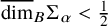 for every irrational
$\alpha $
for every irrational
$\alpha $
 . However, Jitomirskaya and Zhang [Reference Jitomirskaya and Zhang50] disproved this conjecture by demonstrating that if
$\beta (\alpha )> 0$
. However, Jitomirskaya and Zhang [Reference Jitomirskaya and Zhang50] disproved this conjecture by demonstrating that if
$\beta (\alpha )> 0$
 , then
$\overline {\dim }_B\Sigma _{\alpha } = 1$
, then
$\overline {\dim }_B\Sigma _{\alpha } = 1$
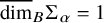 . Here,
$\beta (\alpha )$
. Here,
$\beta (\alpha )$
 measures the Liouvillean property of
$\alpha $
measures the Liouvillean property of
$\alpha $
 and is defined as follows:

where
$q_n(\alpha )$
 denotes the denominator of the n-th convergent of
$\alpha $
denotes the denominator of the n-th convergent of
$\alpha $
 . Note that
$\beta (\alpha ) = 0$
. Note that
$\beta (\alpha ) = 0$
 for every Diophantine
$\alpha $
for every Diophantine
$\alpha $
 , so in particular,
$\beta =0$
, so in particular,
$\beta =0$
 for a.e.
$\alpha $
for a.e.
$\alpha $
 .
.
Considering these results, a natural question arises:
If
$\beta (\alpha ) = 0$
 , what is the box dimension of the spectrum of the critical AMO?
In this paper, we answer this question as follows:
Theorem 1.3. For any
$\delta \in (0,1)$
 , there exists a dense and positive Hausdorff dimension set of
$\alpha \in {\mathbb R}\backslash {\mathbb Q}$
, there exists a dense and positive Hausdorff dimension set of
$\alpha \in {\mathbb R}\backslash {\mathbb Q}$
 with
$\beta (\alpha )=0$
with
$\beta (\alpha )=0$
 , such that the spectrum
$\Sigma _\alpha $
, such that the spectrum
$\Sigma _\alpha $
 of
$H_{1,\alpha ,\theta }$
of
$H_{1,\alpha ,\theta }$
 satisfies

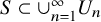
Here the Hausdorff dimension of a set
$S \subset \mathbb {R}$
 is defined as follows:

where an
$\epsilon $
 -cover of S is a family
$(U_n)_n$
-cover of S is a family
$(U_n)_n$
 such that
$S \subset \cup _{n=1}^{\infty } U_n$
such that
$S \subset \cup _{n=1}^{\infty } U_n$
 , and each
$U_n$
, and each
$U_n$
 is an interval of length smaller than
$\epsilon $
is an interval of length smaller than
$\epsilon $
 ;
$|A|$
;
$|A|$
 denotes the Lebesgue measure of
$A\subset {\mathbb R}$
denotes the Lebesgue measure of
$A\subset {\mathbb R}$
 . Indeed, in recent years, there has been an increasing interest in determining the Hausdorff dimension of
$\Sigma _{\alpha }$
. Indeed, in recent years, there has been an increasing interest in determining the Hausdorff dimension of
$\Sigma _{\alpha }$
 . Around 1995, J. BellissardFootnote
1
conjectured that there exists some
$\kappa \in (0, 1/2]$
. Around 1995, J. BellissardFootnote
1
conjectured that there exists some
$\kappa \in (0, 1/2]$
 such that
$\dim _H \Sigma _{\alpha } = \kappa $
such that
$\dim _H \Sigma _{\alpha } = \kappa $
 for almost every
$\alpha $
for almost every
$\alpha $
 . Recently, B. Simon included the problem of determining the Hausdorff dimension of the spectrum of the critical almost Mathieu operator in his new list of significant unsolved problems [Reference Simon67].
Let us review the advances related to these conjectures and provide comments on Theorem 1.3. We introduce the set

In 1994, Last proved that for a dense subset containing
$\mathcal {L}$
 , the Hausdorff dimension of
$\Sigma _{\alpha }$
, the Hausdorff dimension of
$\Sigma _{\alpha }$
 satisfies
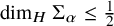
$\dim _H \Sigma _{\alpha } \leq \frac {1}{2}$
satisfies
$\dim _H \Sigma _{\alpha } \leq \frac {1}{2}$
 . This conclusion was recently strengthened by Jitomirskaya and Krasovsky [Reference Jitomirskaya and Krasovsky49] to include all
$\alpha $
. This conclusion was recently strengthened by Jitomirskaya and Krasovsky [Reference Jitomirskaya and Krasovsky49] to include all
$\alpha $
 . Last and Shamis [Reference Last and Shamis58] showed that there exists a dense subset of
$\mathcal {L}$
. Last and Shamis [Reference Last and Shamis58] showed that there exists a dense subset of
$\mathcal {L}$
 for which
$\dim _H \Sigma _{\alpha } = 0$
for which
$\dim _H \Sigma _{\alpha } = 0$
 . The results in [Reference Last and Shamis58] were further enhanced by Avila, Last, Shamis, and Zhou [Reference Avila, Last, Shamis and Zhou11], who established that for any
$\alpha \in \mathcal {L}$
. The results in [Reference Last and Shamis58] were further enhanced by Avila, Last, Shamis, and Zhou [Reference Avila, Last, Shamis and Zhou11], who established that for any
$\alpha \in \mathcal {L}$
 ,
$\dim _H \Sigma _{\alpha } = 0$
,
$\dim _H \Sigma _{\alpha } = 0$
 . However, the box (resp. Hausdorff) dimension may depend sensitively on the arithmetic properties of
$\alpha $
. However, the box (resp. Hausdorff) dimension may depend sensitively on the arithmetic properties of
$\alpha $
 . To illustrate this, let us fix any
$\delta \in (0,1)$
. To illustrate this, let us fix any
$\delta \in (0,1)$
 and define two sets of frequencies as follows:

It is evident that
$\mathscr {F}_B(\delta ) \subset \mathscr {F}_H(\delta )$
 , since for any set
$A \subset [0,1]$
, since for any set
$A \subset [0,1]$
 , it holds that
$\dim _H A \leq \overline {\dim }_B A$
, it holds that
$\dim _H A \leq \overline {\dim }_B A$
 . Moreover, we have
$\mathscr {F}_B(\delta ) \subsetneq \mathscr {F}_H(\delta )$
. Moreover, we have
$\mathscr {F}_B(\delta ) \subsetneq \mathscr {F}_H(\delta )$
 , as [Reference Avila, Last, Shamis and Zhou11] implies that
$\mathcal {L} \subset \mathscr {F}_H(\delta )$
, as [Reference Avila, Last, Shamis and Zhou11] implies that
$\mathcal {L} \subset \mathscr {F}_H(\delta )$
 , while [Reference Jitomirskaya and Zhang50] indicates that
$\mathscr {F}_B(\delta ) \cap \mathcal {L} = \emptyset $
, while [Reference Jitomirskaya and Zhang50] indicates that
$\mathscr {F}_B(\delta ) \cap \mathcal {L} = \emptyset $
 . On the other hand, Helffer-Liu-Qu-Zhou [Reference Helffer, Liu, Qu and Zhou42] illustrated the existence of dense frequencies (with positive Hausdorff dimension) in the set
$\mathbb {R} \setminus \mathcal {L}$
. On the other hand, Helffer-Liu-Qu-Zhou [Reference Helffer, Liu, Qu and Zhou42] illustrated the existence of dense frequencies (with positive Hausdorff dimension) in the set
$\mathbb {R} \setminus \mathcal {L}$
 , such that
$\dim _H \Sigma _{\alpha }> 0$
, such that
$\dim _H \Sigma _{\alpha }> 0$
 . Theorem 1.3 is a consequence of the following:
Theorem 1.4. For any
$\delta> 0$
 , the sets
$\mathscr {F}_B(\delta )$
, the sets
$\mathscr {F}_B(\delta )$
 and
$\mathscr {F}_H(\delta )$
and
$\mathscr {F}_H(\delta )$
 are dense in
${\mathbb R}$
are dense in
${\mathbb R}$
 and of positive Hausdorff dimension.
1.4 Ideas of the proof
The semiclassical analysis of
$M_{\cos ,\vec {\alpha }}$
 was established in [Reference Assel1]; however, the estimates provided there are too crude to yield precise spectral information. For multidimensional Schrödinger operators with separable potentials as defined in (1.5), their spectra can be expressed as Minkowski sums of one-dimensional spectra. In the limit-periodic case, Damanik, Fillman, and Gorodetski [Reference Damanik, Fillman and Gorodetski24] constructed a Cantor spectrum by analyzing a one-dimensional limit-periodic Schrödinger operator with a spectrum of lower box dimension zero; then the result follows from standard arguments about Minkowski sums of fractal sets. Their methodology, however, fails in our context due to the positivity of the Hausdorff dimension. To address this, we explicitly prove that the upper box dimension can be made arbitrarily small (Theorem 1.4), which forces the Minkowski sum to have Lebesgue measure zero (Theorem 1.1). The crux of the proof lies in Theorem 1.4, whose analysis relies on the semiclassical analysis of the almost Mathieu operator (AMO) developed by Helffer and Sjöstrand [Reference Helffer and Sjöstrand43, Reference Helffer and Sjöstrand44, Reference Helffer and Sjöstrand45], which will be shortly recalled in the appendices.
1.4.1 Structure of the spectrum
In our previous work [Reference Helffer, Liu, Qu and Zhou42], we established a lower bound for the Hausdorff dimension of the spectrum for frequencies
$\alpha = [a_1, a_2, \ldots ]$
 where
$a_n$
where
$a_n$
 is eventually sufficiently large. Our work is based on the fine covering structure of the spectrum established in [Reference Helffer and Sjöstrand43, Reference Helffer and Sjöstrand44]. In [Reference Helffer and Sjöstrand43], Helffer and Sjöstrand inductively constructed a family of nested coverings
$\{\mathcal {B}_n: n \in \mathbb {N}\}$
is eventually sufficiently large. Our work is based on the fine covering structure of the spectrum established in [Reference Helffer and Sjöstrand43, Reference Helffer and Sjöstrand44]. In [Reference Helffer and Sjöstrand43], Helffer and Sjöstrand inductively constructed a family of nested coverings
$\{\mathcal {B}_n: n \in \mathbb {N}\}$
 of the spectrum. Let us fix a small
$\epsilon> 0$
of the spectrum. Let us fix a small
$\epsilon> 0$
 . The covering
$\mathcal {B}_0$
. The covering
$\mathcal {B}_0$
 consists of a single interval (or band)
$B_\emptyset $
consists of a single interval (or band)
$B_\emptyset $
 , which is approximately
$[-4, 4]$
, which is approximately
$[-4, 4]$
 . The covering
$\mathcal {B}_1$
. The covering
$\mathcal {B}_1$
 is a disjoint family of subintervals of
$B_\emptyset $
is a disjoint family of subintervals of
$B_\emptyset $
 defined as follows:

where
$B_0 = [-\epsilon , \epsilon ]$
 and
and

(Here and later in the introduction,
$a \sim b$
 roughly means that a and b have the same order. However we warn that it is not so precise and we make it vague on purpose for the moment; the exact meaning will be made precise, see especially Definition 3.2.) See Figure 1 for an illustration. Here,
$B_0$
roughly means that a and b have the same order. However we warn that it is not so precise and we make it vague on purpose for the moment; the exact meaning will be made precise, see especially Definition 3.2.) See Figure 1 for an illustration. Here,
$B_0$
 is considered a “black box” in the sense that complete information about its internal structure is unavailable. The construction of
$\mathcal {B}_2$
is considered a “black box” in the sense that complete information about its internal structure is unavailable. The construction of
$\mathcal {B}_2$
 proceeds as follows: for each
$i \neq 0$
proceeds as follows: for each
$i \neq 0$
 , there exists a disjoint family of subintervals of
$B_i$
, there exists a disjoint family of subintervals of
$B_i$
 given by

with
$B_{i0}$
 positioned in the “middle” of
$B_i$
positioned in the “middle” of
$B_i$
 and satisfying
$|B_{i0}|/|B_i| \sim \epsilon $
and satisfying
$|B_{i0}|/|B_i| \sim \epsilon $
 , such that

Again,
$B_{i0}$
 is treated as a black box. The second-order covering is then defined as

For each interval in
$\mathcal {B}_2$
 that is not a black box, the above construction can be repeated. By aggregating all resulting intervals, we obtain
$\mathcal {B}_3$
that is not a black box, the above construction can be repeated. By aggregating all resulting intervals, we obtain
$\mathcal {B}_3$
 , and so forth.
The covering
${\mathcal B}_1$
 and zoom-in of
$B_i$
and zoom-in of
$B_i$
 .
.

Figure 1 Long description
The diagram consists of two parallel horizontal sequences. The upper sequence, labeled B sub empty set, starts at B sub negative p on the far left, followed by B sub negative 2, B sub negative 1, minus epsilon, B sub 0, epsilon, B sub 1, B sub 2, B sub i, and ends at B sub q on the far right. Red squares mark each node, and two thick black rectangles are positioned at minus epsilon and epsilon. Dashed red arrows connect B sub i on the upper sequence to B sub i q i on the lower sequence, and from B sub negative p to B sub i negative p i. The lower sequence, starting at B sub i negative p i, continues with B sub i negative 2, B sub i negative 1, B sub i 0, B sub i 1, B sub i 2, and ends at B sub i q i. Each node in the lower sequence is also marked by a red square. Dashed red lines indicate correspondence between specific nodes in the upper and lower sequences.
For each n, if we disregard all black boxes in
$\mathcal {B}_n$
 and denote the new family as
$\mathcal {B}_n^*$
and denote the new family as
$\mathcal {B}_n^*$
 , we establish a nested covering structure
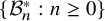
$\{\mathcal {B}_n^*: n \geq 0\}$
, we establish a nested covering structure
$\{\mathcal {B}_n^*: n \geq 0\}$
 . The limit set X of this covering structure satisfies

Using the precise information given by (1.8) and (1.9), we can estimate the lower bound of the Hausdorff dimension of the spectrum.
However, to derive an upper bound for the upper box dimension of the spectrum, partial information about the structure of the spectrum
$\Sigma _\alpha $
 is not sufficient; one must understand how the black boxes evolve during each semiclassical approximation procedure. This is precisely what Helffer and Sjöstrand accomplished in [Reference Helffer and Sjöstrand45]. We will elucidate the situation concerning the first black box
$B_0 = [-\epsilon , \epsilon ]$
is not sufficient; one must understand how the black boxes evolve during each semiclassical approximation procedure. This is precisely what Helffer and Sjöstrand accomplished in [Reference Helffer and Sjöstrand45]. We will elucidate the situation concerning the first black box
$B_0 = [-\epsilon , \epsilon ]$
 , see Figure 2 for an illustration. In [Reference Helffer and Sjöstrand45], Helffer and Sjöstrand replaced the black box
$B_0$
, see Figure 2 for an illustration. In [Reference Helffer and Sjöstrand45], Helffer and Sjöstrand replaced the black box
$B_0$
 with a family of subintervals
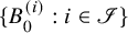
$\{B_0^{(i)}: i \in \mathscr {I}\}$
with a family of subintervals
$\{B_0^{(i)}: i \in \mathscr {I}\}$
 , for which they maintained exact control over
$\# \mathscr {I}$
, for which they maintained exact control over
$\# \mathscr {I}$
 and the ratios
$|B_0^{(i)}|/|B_\emptyset |$
and the ratios
$|B_0^{(i)}|/|B_\emptyset |$
 , similar to (1.8) and (1.9). More specifically, we introduce
$ h \sim 1/a_1$
, similar to (1.8) and (1.9). More specifically, we introduce
$ h \sim 1/a_1$
 and fix a constant
$M> 1$
and fix a constant
$M> 1$
 . Define

Then
$0\in \mathscr I_{in}$
 and
$B_0^{(0)}$
and
$B_0^{(0)}$
 is at the center of
$B_0$
is at the center of
$B_0$
 , of size h, and is the largest subinterval. For
$i\in \mathscr I_{in}\setminus \{0\}$
, of size h, and is the largest subinterval. For
$i\in \mathscr I_{in}\setminus \{0\}$
 ,
,

For the bands in
$B_0 \setminus [-Mh, Mh]$
 , the lengths decrease progressively, ranging roughly from
$-h/\log h$
, the lengths decrease progressively, ranging roughly from
$-h/\log h$
 to
$e^{-1/h}$
to
$e^{-1/h}$
 . The exact description is a bit complex, we refer the reader to Definition 3.2 (vi). It is in this part that the bands exhibit typical multiscale nature. Consequently, we obtain an upgraded covering

such that for the pair
$(B_\emptyset , \tilde {\mathcal {B}}_1)$
 , we possess complete information regarding the cardinality of
$\tilde {\mathcal {B}}_1$
, we possess complete information regarding the cardinality of
$\tilde {\mathcal {B}}_1$
 and the ratios
$|B|/|B_\emptyset |$
and the ratios
$|B|/|B_\emptyset |$
 for all
$B \in \tilde {\mathcal {B}}_1$
for all
$B \in \tilde {\mathcal {B}}_1$
 . This motivates our definition of a special type of configuration, which will be explicitly detailed in Section 3.
The black box
$B_0$
 .
.

Figure 2 Long description
From left to right, the horizontal axis is bounded by minus epsilon and epsilon. Green blocks represent j in I sub mid, grouped on both sides of the central region. The central region, labeled I sub in, contains yellow blocks between minus M h and M h, with boundaries B zero super i and B zero super zero. The entire interval is denoted B zero, spanning all regions. Dashed lines above the axis indicate corresponding intervals for each block. Labels B zero super j and B zero super j prime mark the boundaries of the green regions. The arrangement visually separates the mid and in sets, with color and bracket annotations clarifying group membership.
The strength of [Reference Helffer and Sjöstrand45] lies in the ability to iterate this process. The authors introduce two types. Specifically, starting from any band B in
$\tilde {\mathcal {B}}_1$
 with a certain type, one can repeat the aforementioned construction to obtain another pair
$(B, \tilde {\mathcal {B}}_B)$
with a certain type, one can repeat the aforementioned construction to obtain another pair
$(B, \tilde {\mathcal {B}}_B)$
 , which either behaves essentially the same as
$(B_\emptyset , \tilde {\mathcal {B}}_1)$
, which either behaves essentially the same as
$(B_\emptyset , \tilde {\mathcal {B}}_1)$
 if B has type
$\mathbf {1}$
if B has type
$\mathbf {1}$
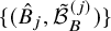
 , or can be decomposed into finitely many (with uniform upper bound) pairs
$\{(\hat {B}_j, \tilde {\mathcal {B}}_B^{(j)})\}$
, or can be decomposed into finitely many (with uniform upper bound) pairs
$\{(\hat {B}_j, \tilde {\mathcal {B}}_B^{(j)})\}$
 , each of which behaves similarly to
$(B_\emptyset , \tilde {\mathcal {B}}_1)$
, each of which behaves similarly to
$(B_\emptyset , \tilde {\mathcal {B}}_1)$
 if B has type
$\mathbf {2}$
if B has type
$\mathbf {2}$
 (see also Definitions B.2 and B.4). In this manner, we can construct
$\tilde {{\mathcal B}}_2$
(see also Definitions B.2 and B.4). In this manner, we can construct
$\tilde {{\mathcal B}}_2$
 , ensuring a precise control over the cardinality of
$\tilde {{\mathcal B}}_2$
, ensuring a precise control over the cardinality of
$\tilde {{\mathcal B}}_2$
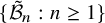
 and the ratios of lengths between any band and its sub-bands. This process can be continued to construct the entire family
$\{\tilde {\mathcal {B}}_n: n \geq 1\}$
and the ratios of lengths between any band and its sub-bands. This process can be continued to construct the entire family
$\{\tilde {\mathcal {B}}_n: n \geq 1\}$
 . With this family established, we can ultimately estimate the upper bound of the upper box dimension of the spectrum.
1.4.2 Estimate the fractal dimensions
In [Reference Helffer and Sjöstrand44, Reference Helffer and Sjöstrand45], it was established that the spectrum
$\Sigma _\alpha $
 is a Cantor set. Furthermore, [Reference Helffer and Sjöstrand45] suggested that this result might enable a detailed analysis of the Hausdorff dimension of
$\Sigma _\alpha $
is a Cantor set. Furthermore, [Reference Helffer and Sjöstrand45] suggested that this result might enable a detailed analysis of the Hausdorff dimension of
$\Sigma _\alpha $
 . The present work realizes this suggestion by providing a concrete study of the Hausdorff dimension, even its box dimension.
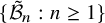
To estimate the fractal dimensions of
$\Sigma _\alpha $
 , we analyze the nested covering structure
$\{\tilde {\mathcal {B}}_n : n \geq 1\}$
, we analyze the nested covering structure
$\{\tilde {\mathcal {B}}_n : n \geq 1\}$
 . While this structure shares similarities with the Moran sets studied in [Reference Feng, Wen and Wu28], it exhibits greater complexity. Specifically, the spectrum can be interpreted as a nonlinear, graph-directed, and highly nonhomogeneous variant of a Moran set.
Estimating the upper bound for the Hausdorff dimension is relatively straightforward due to the natural covering of the spectrum provided by each
$\tilde {\mathcal {B}}_n$
 . Given the precise metrical information encoded in these coverings, deriving this bound requires only standard arguments. In contrast, the upper box dimension poses significant challenges. For fixed
$r> 0$
. Given the precise metrical information encoded in these coverings, deriving this bound requires only standard arguments. In contrast, the upper box dimension poses significant challenges. For fixed
$r> 0$
 , one has to estimate
$N_r(\Sigma _\alpha )$
, one has to estimate
$N_r(\Sigma _\alpha )$
 , the minimal number of intervals of length r needed to cover
$\Sigma _\alpha $
, the minimal number of intervals of length r needed to cover
$\Sigma _\alpha $
 . The difficulty arises from the multiscale structure of the bands in
$\tilde {\mathcal {B}}_B$
. The difficulty arises from the multiscale structure of the bands in
$\tilde {\mathcal {B}}_B$
 : the configuration
$(B, \tilde {\mathcal {B}}_B)$
: the configuration
$(B, \tilde {\mathcal {B}}_B)$
 exhibits pronounced nonhomogeneity in band lengths.
A critical insight resolves this issue: by imposing an upper bound on the coefficients
$a_n$
 , we ensure a lower bound on the length ratio between the shortest band in
$\tilde {\mathcal B}_B$
, we ensure a lower bound on the length ratio between the shortest band in
$\tilde {\mathcal B}_B$
 and
$B.$
and
$B.$
 This constraint allows us to effectively control
$N_r(\Sigma _\alpha )$
This constraint allows us to effectively control
$N_r(\Sigma _\alpha )$
 , thereby bounding the upper box dimension.
Finally, let us explain why the upper box dimension of the spectrum can be made arbitrarily small. Recall that for a self-similar set S with open set condition, the Hausdorff and box dimensions are equal and the common value s is determined through
$\sum _{i=1}^k c_i^s=1$
 , where
$c_i$
, where
$c_i$
 is the i-th contraction ratio. By analogy with this, if for any small
$\delta \in (0,1)$
is the i-th contraction ratio. By analogy with this, if for any small
$\delta \in (0,1)$
 and a typical configuration like
$(B_\emptyset , \tilde {\mathcal B}_1)$
and a typical configuration like
$(B_\emptyset , \tilde {\mathcal B}_1)$
 , we have

then we can use a similar argument to show that the Hausdorff dimension of the spectrum is less than
$\delta $
 . If in addition,
$\{a_n:n\in {\mathbb N}\}$
. If in addition,
$\{a_n:n\in {\mathbb N}\}$
 is bounded from above, then the upper box dimension of the spectrum is also less than
$\delta $
is bounded from above, then the upper box dimension of the spectrum is also less than
$\delta $
 . By the definition of
$\tilde {\mathcal B}_1$
. By the definition of
$\tilde {\mathcal B}_1$
 , we can write

By (1.8) and (1.10), it is seen that for
$a_1$
 large enough (equivalent, for h small enough), we have
$S_{out}(\delta )<1/3$
large enough (equivalent, for h small enough), we have
$S_{out}(\delta )<1/3$
 and
$S_{in }(\delta )<1/3$
and
$S_{in }(\delta )<1/3$
 . But for
$S_{mid}(\delta )$
. But for
$S_{mid}(\delta )$
 , there is no easy path to get the estimate. We need to decompose the sum according to the different scales and estimate them separately. Although quite tricky, it turns out that one can choose suitable h such that
$S_{mid}(\delta )<1/3.$
, there is no easy path to get the estimate. We need to decompose the sum according to the different scales and estimate them separately. Although quite tricky, it turns out that one can choose suitable h such that
$S_{mid}(\delta )<1/3.$
 Consequently, we obtain the desired estimates.
The above argument assumes
$a_n$
 is large for all
$n \geq 1$
is large for all
$n \geq 1$
 . To extend these fractal dimension estimates to a dense set of frequencies
$\alpha $
. To extend these fractal dimension estimates to a dense set of frequencies
$\alpha $
 , we relax this condition: it suffices for them that there exists
$m \in \mathbb {N}$
, we relax this condition: it suffices for them that there exists
$m \in \mathbb {N}$
 such that
$a_n$
such that
$a_n$
 is sufficiently large for all
$n \geq m$
is sufficiently large for all
$n \geq m$
 . To achieve this, we need the full strength of [Reference Helffer and Sjöstrand44] and to extend slightly [Reference Helffer and Sjöstrand45]. For details, we refer the reader to Appendix C.
1.5 Outline of the paper
The rest of the paper is organized as follows. In Section 2, we prove Theorem 1.1 by assuming Theorem 1.4. In Section 3, we define certain abstract configurations and study their basic properties. In Section 4, we define an abstract nested covering structure and obtain the upper bound estimates of the Hausdorff and upper box dimensions of the limit set. In Section 5, we apply the result established in Section 4 to the critical AMO and prove Theorem 1.4 and Theorem 1.3. In Appendices A, B, and C we extract from [Reference Helffer and Sjöstrand43, Reference Helffer and Sjöstrand44, Reference Helffer and Sjöstrand45] what we need for the description of the nested covering structure.
2 Proof of Theorem 1.1
In this section, we prove Theorem 1.1, which is a direct consequence of Theorem 1.4. The proof of Theorem 1.4 is considerably more involved and will be given in Section 5.
Let us recall some known facts from fractal geometry.
Lemma 2.1 [Reference Falconer27].
Assume
$A_1,\cdots , A_d\subset {\mathbb R}$
 are nonempty. Then
(1)
$\sum _{i=1}^{d}\dim _H A_i\le \dim _H \Big (\prod _{i=1}^{d}A_i\Big ).$

(2) If
$A_i, 1\le i\le d$
 are bounded, then

Proof. (1) See [Reference Falconer27] Product Formula 7.2.
(2) See [Reference Falconer27] Product Formula 7.5 for the second inequality. Define the map
$P:{\mathbb R}^d\to {\mathbb R}$
 as
$P(x_1,\cdots ,x_d):=\sum _{i=1}^{d}x_i$
as
$P(x_1,\cdots ,x_d):=\sum _{i=1}^{d}x_i$
 . Then P is Lipschitz. By [Reference Falconer27] Section 3.2(iv), we have

So (2) holds.
In the following discussion, when considering any self-adjoint operator
$ H $
 defined on a Hilbert space
$ \mathcal {H} $
defined on a Hilbert space
$ \mathcal {H} $
 (
$ \mathcal {H}$
(
$ \mathcal {H}$
 usually denotes
$\ell ^2(\mathbb {Z}^d) $
usually denotes
$\ell ^2(\mathbb {Z}^d) $
 or
$ L^2(\mathbb {R}) $
or
$ L^2(\mathbb {R}) $
 ), we denote the spectrum of
$ H $
), we denote the spectrum of
$ H $
 by
$ \mathrm {Sp}(H) $
by
$ \mathrm {Sp}(H) $
 and continue to use
$ \Sigma _{\alpha } $
and continue to use
$ \Sigma _{\alpha } $
 to represent the spectrum of the critical AMO.
Proof of Theorem 1.1.
Fix
$\delta =1/(d+1)$
 . Define

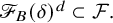
We claim that:
$\mathscr F_B(\delta )^d\subset \mathcal F.$
 Indeed, for any
$\vec \alpha =(\alpha _1,\cdots ,\alpha _d)\in \mathscr F_B(\delta )^d,$
Indeed, for any
$\vec \alpha =(\alpha _1,\cdots ,\alpha _d)\in \mathscr F_B(\delta )^d,$
 by [Reference Damanik and Gorodetski22] Proposition 6.1 (a), we have

Since
$\alpha _i\in \mathscr F_B(\delta )$
 , by Lemma 2.1(2),

Consequently
$|\mathrm {Sp}(M_{\cos ,\vec \alpha })|=0.$
 So the claim holds.
By Theorem 1.4,
$\mathscr F_B(\delta )$
 is dense in
${\mathbb R}$
is dense in
${\mathbb R}$
 and
$\dim _H \mathscr F_B(\delta )>0$
and
$\dim _H \mathscr F_B(\delta )>0$
 . So we conclude that
$\mathscr F_B(\delta )^d$
. So we conclude that
$\mathscr F_B(\delta )^d$
 is dense in
${\mathbb R}^d$
is dense in
${\mathbb R}^d$
 . By Lemma 2.1(1), we have
$\dim _H \Big ( \mathscr F_B(\delta )^d\Big ) \ge d \dim _H\mathscr F_B(\delta )>0.$
. By Lemma 2.1(1), we have
$\dim _H \Big ( \mathscr F_B(\delta )^d\Big ) \ge d \dim _H\mathscr F_B(\delta )>0.$
 Then by the claim,
$\mathcal F$
Then by the claim,
$\mathcal F$
 is dense in
${\mathbb R}^d$
is dense in
${\mathbb R}^d$
 and has positive Hausdorff dimension. So
$\mathcal F+{\mathbb Z}^d\subset {\mathbb T}^d$
and has positive Hausdorff dimension. So
$\mathcal F+{\mathbb Z}^d\subset {\mathbb T}^d$
 is dense in
${\mathbb T}^d$
is dense in
${\mathbb T}^d$
 and has positive Hausdorff dimension.
3 Configurations and their basic properties
In this section, we define several configurations related to an interval and a family of its subintervals. They are abstractions from the covering structure of the spectrum via one step of semiclassical approximation, as we explained in Paragraph 1.4.1. We also study its basic properties, which will be useful later for estimating the dimensions of the spectrum.
3.1 Primitive configuration
At first, we introduce some notation.
Given two intervals
$I=[a,b]$
 and
$J=[c,d]$
and
$J=[c,d]$
 , we write
$I<J$
, we write
$I<J$
 if
$b<c.$
if
$b<c.$
 Assuming that
$\mathcal J$
Assuming that
$\mathcal J$
 is a finite family of compact intervals, we write:

Definition 3.1. If I is a compact interval and
$\mathcal J$
 is a finite class of disjoint subintervals of I, we call
$(I,\mathcal J)$
is a finite class of disjoint subintervals of I, we call
$(I,\mathcal J)$
 a configuration. If moreover,
$\#\mathcal J\ge 3$
a configuration. If moreover,
$\#\mathcal J\ge 3$
 and we index
$\mathcal J$
and we index
$\mathcal J$
 as
as

such that
$J_i< J_{i+1}$
 for any
$-r\le i<s$
for any
$-r\le i<s$
 , then we call
$(I,\mathcal J)$
, then we call
$(I,\mathcal J)$
 a
$[r,s]$
a
$[r,s]$
 -configuration.
Assume
$(I,\mathcal J)$
 is a
$[r,s]$
is a
$[r,s]$
 -configuration. For any
$1\le i\le s$
-configuration. For any
$1\le i\le s$
 , we denote the gap between
$J_{i-1}$
, we denote the gap between
$J_{i-1}$
 and
$J_i$
and
$J_i$
 by
$G_i$
by
$G_i$
 . For any
$1\le i\le r$
. For any
$1\le i\le r$
 , we denote the gap between
$J_{-i}$
, we denote the gap between
$J_{-i}$
 and
$J_{-i+1}$
and
$J_{-i+1}$
 by
$G_{-i}$
by
$G_{-i}$
 . See Figure 3 for an illustration.
A
$[r,s]$
 -configuration.

Figure 3 Long description
The diagram consists of a horizontal blue line with evenly spaced red rectangular blocks. Below each block, labels run from left to right as J sub minus r, J sub minus r plus 1, J sub minus 2, J sub minus 1, J sub 0, J sub 1, J sub 2, J sub s minus 1, and J sub s. Above each pair or group of blocks, curly brackets indicate groupings labeled G sub minus r, G sub minus 2, G sub minus 1, G sub 1, G sub 2, and G sub s, corresponding to the blocks below. A large blue bracket labeled I spans the entire sequence from J sub minus r to J sub s. Dashed red lines indicate omitted or skipped segments between J sub minus r plus 1 and J sub minus 2, and between J sub 2 and J sub s minus 1.
3.2 Configurations with metrical control
The following definition is strongly motivated by the pair
$(B_\emptyset , \tilde {\mathcal B}_1)$
 mentioned in Paragraph 1.4.1. See Figure 4 for an illustration of the definition.
Definition 3.2. Given a
$[r,s]$
 -configuration
$(I,\mathcal J)$
-configuration
$(I,\mathcal J)$
 . Write
$\mathscr I:=\{i\in {\mathbb Z}:-r\le i\le s\}$
. Write
$\mathscr I:=\{i\in {\mathbb Z}:-r\le i\le s\}$
 and
and

Given the following parameters:

$(I,\mathcal J)$
 is called a standard
$(\varsigma ,\epsilon , M, C,h)$
is called a standard
$(\varsigma ,\epsilon , M, C,h)$
 -configuration if the following hold:
A standard configuration from far away.

Figure 4 Long description
Starting at the far left, the axis begins at negative four, eta with a blue dashed line and red vertical bars marking the out region, labeled out in italic above. The next segment, mid, is indicated by green brackets and green vertical bars, spanning from negative epsilon to negative M h. The central in region, highlighted in yellow, extends from negative M h to M h and contains yellow vertical bars and rectangles. To the right, another mid region mirrors the left, marked by green brackets and bars, from M h to epsilon. The final out region, again marked in red, extends from epsilon to xi, four. Above the entire sequence, a blue bracket labeled I spans all five regions. All region labels are in italic. The axis is annotated with negative four, eta negative epsilon, negative M h, M h, epsilon, and xi, four at key transitions.
(i) I satisfies

(ii) The numbers
$r,s$
 satisfy

(iii) The “central,” leftmost, and rightmost subintervals satisfy

(iv) Write
$r_1:=-\min \mathscr I_{in}, s_1=\max \mathscr I_{in}$
 , where

We have

Moreover, for any
$i\in \mathscr I_{in}\setminus \{0\}$
 , we have

(v) Write
$\mathscr I_{out}:=\mathscr I_{out}^-\bigsqcup \mathscr I_{out}^+$
 , where

Then for any
$i\in \mathscr I_{out}$
 , we have

(vi) For any
$i\in \mathscr I_{mid}:=\mathscr I\setminus (\mathscr I_{in}\cup \mathscr I_{out})$
 , we have

where
$c_i$
 and
$g_i$
and
$g_i$
 are the centers of
$J_i$
are the centers of
$J_i$
 and
$G_i$
and
$G_i$
 , respectively.
See Figures 5, 6, 7 for geometric illustrations of
$(iv), (v), (vi),$
 respectively.
Zoom-in of the inside part.

Figure 5 Long description
From the far left, the diagram begins with minus M h above a bracket that spans leftward segments labeled G sub minus r sub 1 and J sub minus r sub 1. Moving right, the next segments are G sub minus 2, G sub minus 1, J sub minus 2, and J sub minus 1, each paired with a yellow square. At the center is J zero, a longer yellow rectangle. To the right of center, the sequence continues with J sub 1, J sub 2, G sub 1, and G sub 2, each with corresponding yellow squares. The far right segment is labeled G sub s sub 1 and J sub s sub 1, under a bracket labeled M h. Above the central region, a large bracket labeled i n spans from minus M h to M h. Dashed yellow lines connect the outermost yellow squares to the central region.
Zoom-in of the right outside part, where
$s_2=\min \mathscr I_{out}^+$
 .
.

Zoom-in of the right middle part.

Let us first make some simple observations that will be useful later.
Lemma 3.3. Assume
$\varsigma ,\epsilon , M,C$
 satisfy (3.1). Then there exists
$\hat h=\hat h(C)>0$
satisfy (3.1). Then there exists
$\hat h=\hat h(C)>0$
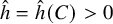 such that if
$h\in (0,\hat h]$
such that if
$h\in (0,\hat h]$
 and
$(I,\mathcal J) $
and
$(I,\mathcal J) $
 is a standard
$(\varsigma ,\epsilon , M,C,h)$
is a standard
$(\varsigma ,\epsilon , M,C,h)$
 -configuration, then

Proof. Choose
$\hat h=\hat h(C)>0$
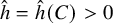 such that for any
$h\in (0,\hat h]$
such that for any
$h\in (0,\hat h]$
 , we have

Notice that if
$i\in \mathscr I_{mid}$
 , then

So if
$h\in (0,\hat h]$
 , by Definition 3.2 and (3.3),

So (3.2) holds.
To model the more general pair
$(B,\tilde {\mathcal B}_B)$
 which is mentioned in Paragraph 1.4.1, we introduce two more configurations as follows:
Definition 3.4. Assume
$(I,\mathcal J)$
 is a
$[r,s]$
is a
$[r,s]$
 -configuration and
$\varsigma ,\epsilon , M,C, h$
-configuration and
$\varsigma ,\epsilon , M,C, h$
 satisfy (3.1). We call
$(I,\mathcal J)$
satisfy (3.1). We call
$(I,\mathcal J)$
 an
$(\varsigma ,\epsilon , M,C,h)$
an
$(\varsigma ,\epsilon , M,C,h)$
 -configuration if there exists an affine map T such that
$(T(I),T(\mathcal J))$
-configuration if there exists an affine map T such that
$(T(I),T(\mathcal J))$
 is a standard
$(\varsigma ,\epsilon , M, C,h)$
is a standard
$(\varsigma ,\epsilon , M, C,h)$
 -configuration, where
$ T(\mathcal J):=\{T(J): J\in \mathcal J\}. $
-configuration, where
$ T(\mathcal J):=\{T(J): J\in \mathcal J\}. $

Definition 3.5. Assume
$(I,\mathcal J)$
 is a configuration and
$\varsigma ,\epsilon , M,C, h$
is a configuration and
$\varsigma ,\epsilon , M,C, h$
 satisfy (3.1). Assume
$k\in {\mathbb N}$
satisfy (3.1). Assume
$k\in {\mathbb N}$
 and
$\rho \in (0,1)$
and
$\rho \in (0,1)$
 . We call
$(I,\mathcal J)$
. We call
$(I,\mathcal J)$
 a
$(k,\rho ;\varsigma ,\epsilon , M, C,h)$
a
$(k,\rho ;\varsigma ,\epsilon , M, C,h)$
 -configuration if the following hold:
(i) There exists a disjoint family
$\{I_1,\cdots , I_k\}$
 of subintervals of I such that

and for any
$J\in \mathcal J$
 , there exists some i (hence unique) such that
$J\subset I_i$
, there exists some i (hence unique) such that
$J\subset I_i$
 .
.
(ii) For any i, define
$ \mathcal J_i:=\{J\in \mathcal J: J\subset I_i\}. $
 Then
$(I_i,\mathcal J_i)$
Then
$(I_i,\mathcal J_i)$
 is a
$(\varsigma ,\epsilon , M,C,h)$
is a
$(\varsigma ,\epsilon , M,C,h)$
 -configuration.
See Figure 8 for an example of a
$(3,\rho ;\varsigma ,\epsilon , M, C,h)$
 -configuration.
Remark 3.6. (i) We call the family
$\{(I_i,\mathcal J_i):1\le i\le k\}$
 the sub-
$(\varsigma ,\epsilon , M,C,h)$
the sub-
$(\varsigma ,\epsilon , M,C,h)$
 -configurations of
$(I,\mathcal J).$
-configurations of
$(I,\mathcal J).$

A
$(3,\rho ;\varsigma ,\epsilon , M, C,h)$
 -configuration.

(ii) If
$k=1$
 , then a
$(k,\rho ;\varsigma ,\epsilon , M,C,h)$
, then a
$(k,\rho ;\varsigma ,\epsilon , M,C,h)$
 -configuration is just a
$(\varsigma ,\epsilon , M,C,h)$
-configuration is just a
$(\varsigma ,\epsilon , M,C,h)$
 -configuration.
We have the following observation, which is crucial later for estimating the dimensions of the spectrum.
Lemma 3.7. Given
$k\in {\mathbb N}$
 ,
$\rho \in (0,1)$
,
$\rho \in (0,1)$
 . Assume
$\varsigma ,\epsilon , M, C, h$
. Assume
$\varsigma ,\epsilon , M, C, h$
 satisfy (3.1). Assume
$(I,\mathcal J)$
satisfy (3.1). Assume
$(I,\mathcal J)$
 is a
$(k,\rho; \varsigma ,\epsilon ,M,C,h)$
is a
$(k,\rho; \varsigma ,\epsilon ,M,C,h)$
 -configuration. Let
$\hat h$
-configuration. Let
$\hat h$
 be the constant in Lemma 3.3. Then
(1) There exists
$\tilde h=\tilde h(C,\varsigma ,\rho )\in (0,\hat h]$
 such that if
$h\in (0,\tilde h] $
such that if
$h\in (0,\tilde h] $
 , then for any
$J\in \mathcal J$
, then for any
$J\in \mathcal J$
 ,
,

(2) Assume
$h\in (0,\tilde h]$
 . Assume
$r>0$
. Assume
$r>0$
 satisfies
$\mathcal J_{\min }\le r<|I|$
satisfies
$\mathcal J_{\min }\le r<|I|$
 . Then

(3) Fix
$\kappa \in {\mathbb N}.$
 Then for any
$\delta \in (0,1)$
Then for any
$\delta \in (0,1)$
 there exists
$h(\delta )\in (0,\tilde h]$
there exists
$h(\delta )\in (0,\tilde h]$
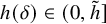 such that if
$h\in (0,h(\delta )]$
such that if
$h\in (0,h(\delta )]$
 and
$1\le k\le \kappa $
and
$1\le k\le \kappa $
 , then

Proof. (1) Define
$\tilde h$
 as
as

Fix any
$h\in (0,\tilde h]$
 . Assume
$J_\ast \in \mathcal J_i$
. Assume
$J_\ast \in \mathcal J_i$
 is such that
$|J_\ast |=\mathcal J_{\min }.$
is such that
$|J_\ast |=\mathcal J_{\min }.$
 By Definition 3.5,
$(I_i,\mathcal J_i)$
By Definition 3.5,
$(I_i,\mathcal J_i)$
 is a
$( \varsigma ,\epsilon ,M,C,h)$
is a
$( \varsigma ,\epsilon ,M,C,h)$
 -configuration and
$|I_i|/|I|\ge \rho /k$
-configuration and
$|I_i|/|I|\ge \rho /k$
 . So by Lemma 3.3,

Similarly, assume
$J^\ast \in \mathcal J_j$
 is such that
$|J^\ast |=\mathcal J_{\max }.$
is such that
$|J^\ast |=\mathcal J_{\max }.$
 By Definition 3.5,
$(I_j,\mathcal J_j)$
By Definition 3.5,
$(I_j,\mathcal J_j)$
 is a
$( \varsigma ,\epsilon ,M,C,h)$
is a
$( \varsigma ,\epsilon ,M,C,h)$
 -configuration and
$|I_j|/|I|\le 1/k\rho $
-configuration and
$|I_j|/|I|\le 1/k\rho $
 . So by Lemma 3.3,

So the result follows.
(2) By (1), we have

(3) Assume
$\{I_1,\cdots ,I_k\}$
 are the subintervals in Definition 3.5(i). Since
$k\le \kappa $
are the subintervals in Definition 3.5(i). Since
$k\le \kappa $
 , we have

By Definition 3.5(ii), each
$(I_i, \mathcal J_i)$
 is a
$(\varsigma ,\epsilon ,M,C,h)$
is a
$(\varsigma ,\epsilon ,M,C,h)$
 -configuration. Thus to get (3.4), we only need to show that for a standard
$(\varsigma ,\epsilon , M, C,h)$
-configuration. Thus to get (3.4), we only need to show that for a standard
$(\varsigma ,\epsilon , M, C,h)$
 -configuration
$(I,\mathcal J)$
-configuration
$(I,\mathcal J)$
 , we have

Now assume
$(I,\mathcal J)$
 is a standard
$(\varsigma ,\epsilon , M, C,h)$
is a standard
$(\varsigma ,\epsilon , M, C,h)$
 -configuration. By Definition 3.2(i), we have
$|I|\ge 2\varsigma $
-configuration. By Definition 3.2(i), we have
$|I|\ge 2\varsigma $
 . To show (3.6), we only need to show that

We split the sum in (3.7) into three parts and estimate them separately. Write

By Definition 3.2(iii) and (iv), we have

By Definition 3.2(ii) and (v), we have

By (3.8) and (3.9) it is seen that there exists
$h_1\in (0,\tilde h]$
 such that for any
$h\in (0,h_1]$
such that for any
$h\in (0,h_1]$
 we have

The estimate of
$S_{mid}(\delta )$
 is more complex. We need to split the sum further according to different scales. We proceed as follows. Assume
$L=L(h)\in {\mathbb N}$
is more complex. We need to split the sum further according to different scales. We proceed as follows. Assume
$L=L(h)\in {\mathbb N}$
 is such that

Recall that
$c_i$
 is the center of
$J_i.$
is the center of
$J_i.$
 For any
$1\le l\le L$
For any
$1\le l\le L$
 , define

Since
$e^{-L-1}<h< Mh\le |c_i|\le \epsilon <e^{-1}$
 , we have

By Definition 3.2(vi), if
$i\in \mathscr I_{mid}^l$
 , we have

Now we estimate the cardinality of
$\mathscr I_{mid}^l$
 . If
$i-1,i\in \mathscr I_{mid}^l$
. If
$i-1,i\in \mathscr I_{mid}^l$
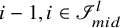 , then

By Definition 3.2(vi), we have

From this we conclude that

Consequently, we have

If
$1\le l\le L(1-\delta /2)$
 , then

If
$ l> L(1-\delta /2)$
 , then

From these, it is seen that there exists
$h(\delta )\in (0,h_1)$
 such that for any
$h\in (0,h(\delta )]$
such that for any
$h\in (0,h(\delta )]$
 and any
$1\le l\le L$
and any
$1\le l\le L$
 we have

Consequently, we have

4 Dimension estimates for the limit set of a nested covering structure
Motivated by the covering structure of the spectrum
$\Sigma _\alpha $
 obtained in [Reference Helffer and Sjöstrand43, Reference Helffer and Sjöstrand44, Reference Helffer and Sjöstrand45], in this section, we define an abstract nested covering structure with the special configurations as their building blocks. This nested covering structure naturally determines a limit set. Due to the fine metrical control of the configurations, we can obtain the upper bounds for the fractal dimensions of the limit set. In the next section, we will apply the result to the spectrum of critical AMO.
4.1 An abstract language
At first we define an abstract language, which will be used as the index set for the abstract nested coverings. It is good to keep in mind that the following definitions are intended to give a coding for a
$(k,\rho; \varsigma ,\epsilon ,M,C,h)$
 -configuration. The types are related to the types of bands in
$\tilde {\mathcal B}_n$
-configuration. The types are related to the types of bands in
$\tilde {\mathcal B}_n$
 (see Paragraph 1.4.1).
We define the alphabet for the types as

Fix some
$\mathbf t\in \{\mathbf {1},\mathbf {2}\}$
 . Define
$\Omega _0$
. Define
$\Omega _0$
 as
as

We call
$\mathbf t$
 the type of the word
$\emptyset _{\mathbf t}$
the type of the word
$\emptyset _{\mathbf t}$
 .
.
Next, we define
$\Omega _1$
 as follows. We fix the only word
$w=\emptyset _{\mathbf t}\in \Omega _0$
as follows. We fix the only word
$w=\emptyset _{\mathbf t}\in \Omega _0$
 . Choose
$k_w\in {\mathbb N}$
. Choose
$k_w\in {\mathbb N}$
 , and for any
$1\le k\le k_w$
, and for any
$1\le k\le k_w$
 , choose
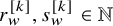
$r_w^{[k]}, s_w^{[k]}\in {\mathbb N}$
, choose
$r_w^{[k]}, s_w^{[k]}\in {\mathbb N}$
 and write

Define the alphabets

Then define

Assume
$\Omega _n$
 has been defined. We define
$\Omega _{n+1}$
has been defined. We define
$\Omega _{n+1}$
 as follows. Fix any
$w\in \Omega _n$
as follows. Fix any
$w\in \Omega _n$
 , choose
$k_w\in {\mathbb N}$
, choose
$k_w\in {\mathbb N}$
 , and for any
$1\le k\le k_w$
, and for any
$1\le k\le k_w$
 , choose
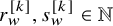
$r_w^{[k]}, s_w^{[k]}\in {\mathbb N}$
, choose
$r_w^{[k]}, s_w^{[k]}\in {\mathbb N}$
 . We write

and define the alphabets

We define
$\Omega _{n+1}$
 as
as

By induction, we have defined a set
$\Omega _n$
 for any
$n\in {\mathbb Z}_+$
for any
$n\in {\mathbb Z}_+$
 . Finally we write

We call
$\Omega _\ast $
 a language and call any
$w\in \Omega _\ast $
a language and call any
$w\in \Omega _\ast $
 a word.
Remark 4.1. In the above definition, the choices of
$k_w, r_w^{[k]}, s_w^{[k]}$
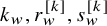 are arbitrary. Meanwhile, as we mentioned, the language serves as the index set for the configurations introduced in Section 3, so natural conditions will be proposed when applying to real situation. One can think
$k_w$
are arbitrary. Meanwhile, as we mentioned, the language serves as the index set for the configurations introduced in Section 3, so natural conditions will be proposed when applying to real situation. One can think
$k_w$
 as the number k in Definition 3.5 and think
$r_w^{[k]}, s_w^{[k]}$
as the number k in Definition 3.5 and think
$r_w^{[k]}, s_w^{[k]}$
 as the numbers
$r,s$
as the numbers
$r,s$
 in Definition 3.2.
For any
$w\in \Omega _\ast $
 and any
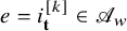
$e=i^{[k]}_{\mathbf t}\in \mathscr A_w$
and any
$e=i^{[k]}_{\mathbf t}\in \mathscr A_w$
 , we call
$\mathbf t, k, i$
, we call
$\mathbf t, k, i$
 the type, the global index, the local index of e, respectively and will use the notations

For any
$w\in \Omega _\ast $
 , we also introduce an order on
$\mathscr A_w$
, we also introduce an order on
$\mathscr A_w$
 as follows: for
$e,\hat e\in \mathscr A_w$
as follows: for
$e,\hat e\in \mathscr A_w$
 and
$e\ne \hat e$
and
$e\ne \hat e$
 ,
,

For any
$w=w_0\cdots w_n\in \Omega _n$
 , we define
$T_w:=T_{w_n}$
, we define
$T_w:=T_{w_n}$
 and say that w has type
$T_{w_n}.$
and say that w has type
$T_{w_n}.$
 We also write
$|w|=n$
We also write
$|w|=n$
 and say that w is a word of length
$n.$
and say that w is a word of length
$n.$
 For any
$0\le i\le n$
For any
$0\le i\le n$
 , we write
$w|_i:=w_0\cdots w_i$
, we write
$w|_i:=w_0\cdots w_i$
 and call it the i-th prefix of
$w.$
and call it the i-th prefix of
$w.$

4.2 A nested covering structure coded by
$\Omega _\ast $

Assuming
$\Omega _\ast $
 is a language defined in the previous subsection, we now describe a nested covering structure indexed by
$\Omega _\ast $
is a language defined in the previous subsection, we now describe a nested covering structure indexed by
$\Omega _\ast $
 .
.
Definition 4.2. Given a language
$\Omega _\ast $
 . Assume
$\mathcal I(\Omega _\ast ):=\{I_w: w\in \Omega _\ast \}$
. Assume
$\mathcal I(\Omega _\ast ):=\{I_w: w\in \Omega _\ast \}$
 is a class of compact intervals in
${\mathbb R}$
is a class of compact intervals in
${\mathbb R}$
 . We say that
$\mathcal I(\Omega _\ast )$
. We say that
$\mathcal I(\Omega _\ast )$
 is a nested covering structure if the following hold:
(i) For any
$w\in \Omega _*$
 , the pair
$(I_w,\mathcal J_w)$
, the pair
$(I_w,\mathcal J_w)$
 is a configuration, where
$\mathcal J_w:=\{I_{we}: e\in \mathscr A_w\}.$
is a configuration, where
$\mathcal J_w:=\{I_{we}: e\in \mathscr A_w\}.$
 Moreover, for different
$e,\hat e\in \mathscr A_w,$
Moreover, for different
$e,\hat e\in \mathscr A_w,$


(ii)
$\max \{|I_w|: w\in \Omega _n\}\to 0$
 as
$n\to \infty $
as
$n\to \infty $
 .
.
Finally, if
$\mathcal I(\Omega _\ast )$
 is a nested covering structure, we define the limit set of
$\mathcal I(\Omega _\ast )$
is a nested covering structure, we define the limit set of
$\mathcal I(\Omega _\ast )$
 as
as

Assume
$\mathcal I(\Omega _\ast )$
 is a nested covering structure. For each
$w\in \Omega _*$
is a nested covering structure. For each
$w\in \Omega _*$
 and
$1\le k\le k_w$
and
$1\le k\le k_w$
 , we write

where
$\mathrm {Co}(A)$
 denotes the convex hull of A. Then
$(I_w^{[k]}, \mathcal J_w^{[k]}), \ 1\le k\le k_w$
denotes the convex hull of A. Then
$(I_w^{[k]}, \mathcal J_w^{[k]}), \ 1\le k\le k_w$
 are all configurations and

4.3 Upper bounds of the dimensions for limit sets
We can now state the main result of this section:
Theorem 4.3. Assume
$\kappa \in {\mathbb N}$
 and
$\rho \in (0,1)$
and
$\rho \in (0,1)$
 . Assume
$\varsigma , \epsilon , M, C$
. Assume
$\varsigma , \epsilon , M, C$
 satisfy (3.1). Fix any
$\delta \in (0,1)$
satisfy (3.1). Fix any
$\delta \in (0,1)$
 , let
$h(\delta )$
, let
$h(\delta )$
 be the constant given by Lemma 3.7(3). Assume
$\Omega _\ast $
be the constant given by Lemma 3.7(3). Assume
$\Omega _\ast $
 is a language and
$\mathcal I(\Omega _\ast )$
is a language and
$\mathcal I(\Omega _\ast )$
 is a nested covering structure such that for any
$w\in \Omega _\ast $
is a nested covering structure such that for any
$w\in \Omega _\ast $
 , there exists
$h_w>0$
, there exists
$h_w>0$
 such that
$(I_w, \mathcal J_w)$
such that
$(I_w, \mathcal J_w)$
 is a
$(k_w,\rho; \varsigma ,\epsilon ,M, C,h_w)$
is a
$(k_w,\rho; \varsigma ,\epsilon ,M, C,h_w)$
 -configuration with
$(I_w^{[k]}, \mathcal J_w^{[k]}), \ 1\le k\le k_w$
-configuration with
$(I_w^{[k]}, \mathcal J_w^{[k]}), \ 1\le k\le k_w$
 as the related sub-
$(\varsigma ,\epsilon ,M,C,h_w)$
as the related sub-
$(\varsigma ,\epsilon ,M,C,h_w)$
 -configurations.
(1) If
$k_w\le \kappa $
 and
$h_w\in (0,h(\delta )]$
and
$h_w\in (0,h(\delta )]$
 for any
$w\in \Omega _\ast $
for any
$w\in \Omega _\ast $
 , then

(2) Fix any
$h'(\delta )\in (0,h(\delta )]$
 . If
$k_w\le \kappa $
. If
$k_w\le \kappa $
 and
$h_w\in [h'(\delta ),h(\delta )]$
and
$h_w\in [h'(\delta ),h(\delta )]$
 for any
$w\in \Omega _\ast $
for any
$w\in \Omega _\ast $
 , then

Proof. (1) For any n,
$\{I_w: w\in \Omega _n\}$
 forms a covering of
$X(\Omega _\ast )$
forms a covering of
$X(\Omega _\ast )$
 . Moreover, by Lemma 3.7(1) we have

We claim that for any
$n\in {\mathbb N},$


We show it by induction. When
$n=0,$
 it is trivially true.
Now assume the statement is true for
$n-1$
 . We have

By the assumption, the pair
$(I_w,\{I_{we}:e\in \mathscr A_w\})$
 is a
$(k_w,\rho ;\varsigma ,\epsilon ,M,C,h_w)$
is a
$(k_w,\rho ;\varsigma ,\epsilon ,M,C,h_w)$
 -configuration with
$k_w\le \kappa $
-configuration with
$k_w\le \kappa $
 and
$h_w\le h(\delta )$
and
$h_w\le h(\delta )$
 . By Lemma 3.7(3), we have

So by induction hypothesis, we have

By induction, the claim holds.
Then by the definition of Hausdorff measure, we have

where
$\mathscr H^\delta $
 denotes
$\delta $
denotes
$\delta $
 -dimensional Hausdorff measure. Consequently,
$\dim _H X(\Omega _\ast )\le \delta .$
-dimensional Hausdorff measure. Consequently,
$\dim _H X(\Omega _\ast )\le \delta .$

(2) Assume
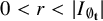
$0<r<|I_{\emptyset _{\mathbf t}}|$
 . Let us estimate
$N_r(X(\Omega _\ast ))$
. Let us estimate
$N_r(X(\Omega _\ast ))$
 . Our strategy is the following: we construct an interval covering of
$X(\Omega _\ast )$
. Our strategy is the following: we construct an interval covering of
$X(\Omega _\ast )$
 such that each interval in this covering is approximately of size r, then we estimate the number of intervals.
First, we define a subset of
$\Omega _\ast $
 as follows. By (4.2), for any
$w\in \Omega _n$
as follows. By (4.2), for any
$w\in \Omega _n$
 we have

Take
$N\in {\mathbb N}$
 such that
$|I_{\emptyset _{\mathbf t}}|/10^N<r.$
such that
$|I_{\emptyset _{\mathbf t}}|/10^N<r.$
 For each
$w\in \Omega _N$
For each
$w\in \Omega _N$
 , let
$0\le m_w\le N$
, let
$0\le m_w\le N$
 be the integer such that

Since
$|I_{\emptyset _{\mathbf t}}|>r$
 and
$|I_w|<r$
and
$|I_w|<r$
 , the number
$m_w$
, the number
$m_w$
 is well-defined and unique. Now define

We claim that:
$\{I_u: u\in \mathcal U\}$
 is a covering of
$X(\Omega _\ast )$
is a covering of
$X(\Omega _\ast )$
 and
$\sum _{u\in \mathcal U}|I_u|^\delta \le |I_{\emptyset _{\mathbf t}}|^\delta .$
and
$\sum _{u\in \mathcal U}|I_u|^\delta \le |I_{\emptyset _{\mathbf t}}|^\delta .$

Indeed, by (4.1),
$\{I_w: w\in \Omega _N\}$
 is a covering of
$X(\Omega _\ast )$
is a covering of
$X(\Omega _\ast )$
 . Since for each
$w\in \Omega _N$
. Since for each
$w\in \Omega _N$
 , we have
$u=w|_{m_w}\in \mathcal U$
, we have
$u=w|_{m_w}\in \mathcal U$
 and
$I_w\subset I_u$
and
$I_w\subset I_u$
 , so the first statement holds.
Notice that if
$u,\hat u\in \mathcal U$
 and
$u\ne \hat u$
and
$u\ne \hat u$
 , then u and
$\hat u$
, then u and
$\hat u$
 are noncompatible, that is, neither
$u\lhd \hat u$
are noncompatible, that is, neither
$u\lhd \hat u$
 nor
$\hat u\lhd u$
nor
$\hat u\lhd u$
 (where
$u\lhd v$
(where
$u\lhd v$
 means that u is a prefix of v). This is due to the uniqueness of
$m_w$
means that u is a prefix of v). This is due to the uniqueness of
$m_w$
 in (4.4). Now write

Then
$0\le m_\ast \le m^\ast \le N.$
 For any
$m_\ast \le k\le m^\ast $
For any
$m_\ast \le k\le m^\ast $
 , write

Then
$\mathcal U=\bigsqcup _{k=m_\ast }^{m^\ast } \mathcal U_k.$
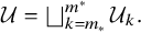 By (4.3) and Lemma 3.7(3), we have

where
$\mathcal V_{m_\ast +1}:=\{ue: u\in \Omega _{m_\ast }\setminus \mathcal U_{m_\ast },e\in \mathscr A_u\}$
 . Since words in
$\mathcal U_{m_\ast +1}$
. Since words in
$\mathcal U_{m_\ast +1}$
 and
$\mathcal U_{m_\ast }$
and
$\mathcal U_{m_\ast }$
 are noncompatible, we must have
$\mathcal U_{m_\ast +1}\subset \mathcal V_{m_\ast +1}.$
are noncompatible, we must have
$\mathcal U_{m_\ast +1}\subset \mathcal V_{m_\ast +1}.$
 Consequently,

We can iterate this process. Finally we get

Hence the second statement of the claim holds.
By (4.4) and the claim, we have

For each
$u\in \mathcal U$
 , since
$(I_u, \mathcal J_u)$
, since
$(I_u, \mathcal J_u)$
 is a
$(k_u,\rho; \varsigma ,\epsilon ,M,C,h_u)$
is a
$(k_u,\rho; \varsigma ,\epsilon ,M,C,h_u)$
 -configuration with
$k_u\le \kappa $
-configuration with
$k_u\le \kappa $
 and
$h'(\delta )\le h_u\le h(\delta )$
and
$h'(\delta )\le h_u\le h(\delta )$
 , by Lemma 3.7(2), we have

Since
$\{I_u: u\in \mathcal U\}$
 is a covering of
$X(\Omega _\ast )$
is a covering of
$X(\Omega _\ast )$
 , we have

Then we have

So the result follows.
5 The fractal dimensions of the spectrum of the critical AMO
In this section, we apply Theorem 4.3 to the critical AMO, thereby completing the proofs of Theorems 1.4 and 1.3.
5.1 The nested covering structure of the spectrum
In this part, the nested covering structure of the spectrum established in [Reference Helffer and Sjöstrand43, Reference Helffer and Sjöstrand44, Reference Helffer and Sjöstrand45] is essential. We summarize the related results in Theorem 5.2. We extract and unify statements from these three works into a form suitable for our application. We will make some remarks on the connection between the result and the works [Reference Helffer and Sjöstrand43, Reference Helffer and Sjöstrand44, Reference Helffer and Sjöstrand45].
Remark 5.1. Note that for
$\alpha ,\beta \in {\mathbb R}\setminus {\mathbb Q}$
 with
$\alpha -\beta \in {\mathbb Z}$
with
$\alpha -\beta \in {\mathbb Z}$
 , we have
$\Sigma _\alpha =\Sigma _\beta $
, we have
$\Sigma _\alpha =\Sigma _\beta $
 . Consequently, both
$\mathscr F_B(\delta )$
. Consequently, both
$\mathscr F_B(\delta )$
 and
$\mathscr F_H(\delta )$
and
$\mathscr F_H(\delta )$
 are
${\mathbb Z}$
are
${\mathbb Z}$
 -invariant. Hence in the rest of this section we will restrict
$\alpha \in [0,1]\setminus {\mathbb Q}.$
-invariant. Hence in the rest of this section we will restrict
$\alpha \in [0,1]\setminus {\mathbb Q}.$

Assume that
$\alpha \in [0,1]\setminus \mathbb {Q}$
 and that it has a continued fraction expansion

Let
$G:[0,1]\setminus \mathbb {Q}\to [0,1] \setminus \mathbb {Q}$
 be the Gauss map defined by

For any
$n\in {\mathbb N}$
 , define

Theorem 5.2 [Reference Helffer and Sjöstrand43, Reference Helffer and Sjöstrand44, Reference Helffer and Sjöstrand45].
Let
$\hat m \in {\mathbb Z}_+$
 and
$\hat M \geq 2$
and
$\hat M \geq 2$
 . Then there exist
$\epsilon _0>0$
. Then there exist
$\epsilon _0>0$
 ,
$ \varsigma \in (0,4)$
,
$ \varsigma \in (0,4)$
 and
$\kappa \in {\mathbb N}$
and
$\kappa \in {\mathbb N}$
 such that, for any
$\epsilon \in (0,\epsilon _0]$
such that, for any
$\epsilon \in (0,\epsilon _0]$
 , there exist
$h_0>0$
, there exist
$h_0>0$
 ,
$M> C> 1$
,
$M> C> 1$
 ,
$\rho \in (0,1)$
,
$\rho \in (0,1)$
 such that if
$\alpha =[a_1,a_2,\cdots ] \in [0,1]\setminus {\mathbb Q}$
such that if
$\alpha =[a_1,a_2,\cdots ] \in [0,1]\setminus {\mathbb Q}$
 satisfies

$q_{\hat m}(\alpha ) $
 is odd, where

is the
$\hat m$
 -th convergent of
$\alpha ,$
-th convergent of
$\alpha ,$
 and
and

then the following hold:
(1) There exists a family of disjoint intervals
$\{I_1,\cdots , I_{q_{\hat m}(\alpha )}\}$
 such that

(2) For each
$1\le i\le q_{\hat m}(\alpha )$
 , there exists a language
$\Omega _\ast ^{(i)}$
, there exists a language
$\Omega _\ast ^{(i)}$
 and a related nested covering structure
$\mathcal I(\Omega _\ast ^{(i)})$
and a related nested covering structure
$\mathcal I(\Omega _\ast ^{(i)})$
 such that the following hold:
(2-1) The limit set of
$\mathcal I(\Omega _\ast ^{(i)})$
 is exactly
$\Sigma _\alpha ^{(i)}$
is exactly
$\Sigma _\alpha ^{(i)}$
 , that is,

(2-2) For each
$n\ge 1$
 and
$w\in \Omega _{n-1}^{(i)}$
and
$w\in \Omega _{n-1}^{(i)}$
 , the pair
$(I_w,\mathcal J_w)$
, the pair
$(I_w,\mathcal J_w)$
 is a
$(k_w,\rho ;\varsigma ,\epsilon ,M,C,h_{n+\hat m}(\alpha ))$
is a
$(k_w,\rho ;\varsigma ,\epsilon ,M,C,h_{n+\hat m}(\alpha ))$
 -configuration with
$k_w\le \kappa $
-configuration with
$k_w\le \kappa $
 , and with

as the related sub-
$(\varsigma ,\epsilon ,M,C,h_{n+\hat m}(\alpha ))$
 -configurations.
(2-3) If
$T_w=\mathbf {1}$
 , then
$k_w=1.$
, then
$k_w=1.$

Proof. We only have to verify that the statement is a direct consequence of the results given in the appendices. This link was already announced in Paragraph 1.4.1. Let us consider step 1 corresponding to the construction of
$\Omega _1$
 . When
$\hat m =0$
. When
$\hat m =0$
 the statement corresponding to the properties of
$\Omega _1$
the statement corresponding to the properties of
$\Omega _1$
 is given in Proposition B.6. For
$a_1$
is given in Proposition B.6. For
$a_1$
 large the semi-classical parameter
$h= 2\pi \alpha $
large the semi-classical parameter
$h= 2\pi \alpha $
 is close to
$2\pi /a_1$
is close to
$2\pi /a_1$
 . The Harper model we are starting from is a type 1f operator and we indeed get a configuration as introduced in Definition 3.2. Theorem B.5 then explains what we shall do in each of the intervals with the new semi-classical parameter
$h'$
. The Harper model we are starting from is a type 1f operator and we indeed get a configuration as introduced in Definition 3.2. Theorem B.5 then explains what we shall do in each of the intervals with the new semi-classical parameter
$h'$
 close to
$2\pi /a_2$
close to
$2\pi /a_2$
 . When
$\hat m>0$
. When
$\hat m>0$
 , the first step is different since we do not start from a type 1 operator but from an h-pseudo-differential system. The analysis performed in [Reference Helffer and Sjöstrand44] (see also Appendices A and B) leads us to a
$(k,\rho ;\varsigma ,\epsilon ,M, C,h)$
, the first step is different since we do not start from a type 1 operator but from an h-pseudo-differential system. The analysis performed in [Reference Helffer and Sjöstrand44] (see also Appendices A and B) leads us to a
$(k,\rho ;\varsigma ,\epsilon ,M, C,h)$
 configuration with
$k= q_{\hat m}(\alpha )$
configuration with
$k= q_{\hat m}(\alpha )$
 (see Figure 8 for an illustration of the configuration when
$\alpha $
(see Figure 8 for an illustration of the configuration when
$\alpha $
 is close to the rational
$1/3$
is close to the rational
$1/3$
 (with
$\hat m=1$
(with
$\hat m=1$
 )). According to the statements in the appendices, we are at step 2 in each interval with a configuration with a new semi-classical parameter
$h'$
)). According to the statements in the appendices, we are at step 2 in each interval with a configuration with a new semi-classical parameter
$h'$
 . Note that k also appears when using Theorem B.7 relative to type
$2$
. Note that k also appears when using Theorem B.7 relative to type
$2$
 operators. We can then iterate at any step.
Remark 5.3. The assumption that
$q_{\hat m}(\alpha )$
 is odd is unessential but permits to assume that the bands corresponding to the spectrum of the Harper model for
$p_{\hat m}(\alpha )/q_{\hat m}(\alpha )$
is odd is unessential but permits to assume that the bands corresponding to the spectrum of the Harper model for
$p_{\hat m}(\alpha )/q_{\hat m}(\alpha )$
 do not touch according to the result of [Reference van Mouche72]. Without this assumption, we should use [Reference Helffer and Sjöstrand44] for the description of the spectrum near the touching point (see the last line in (A.2)) and would require us to change at the first step the definition of
$\tilde {\mathcal B}_1$
do not touch according to the result of [Reference van Mouche72]. Without this assumption, we should use [Reference Helffer and Sjöstrand44] for the description of the spectrum near the touching point (see the last line in (A.2)) and would require us to change at the first step the definition of
$\tilde {\mathcal B}_1$
 (see Paragraph 1.4.1 for the definition of
$\tilde {\mathcal B}_1$
(see Paragraph 1.4.1 for the definition of
$\tilde {\mathcal B}_1$
 ).
).
5.2 Arbitrarily small Hausdorff and upper box dimensions of the spectrum
As an application of Theorem 4.3 and Lemma 3.7, we have the following estimates.
Proposition 5.4. Let
$\hat m \in {\mathbb Z}_+$
 and
$\hat M \geq 2$
and
$\hat M \geq 2$
 . Then for any
$\delta>0$
. Then for any
$\delta>0$
 , there exists a constant
$L:=L(\delta ,\hat m, \hat M)>0$
, there exists a constant
$L:=L(\delta ,\hat m, \hat M)>0$
 such that the following hold:
(1) If
$\alpha =[a_1,a_2,\cdots ,a_{\hat m},a_{\hat m+1},\cdots ]$
 is such that
$q_{\hat m}(\alpha )$
is such that
$q_{\hat m}(\alpha )$
 is odd and

then
$\dim _H\Sigma _\alpha \le \delta $
 .
.
(2) Fix any
$\gamma>1$
 . If
$\alpha =[a_1,a_2,\cdots ,a_{\hat m},a_{\hat m+1},\cdots ]$
. If
$\alpha =[a_1,a_2,\cdots ,a_{\hat m},a_{\hat m+1},\cdots ]$
 is such that
$q_{\hat m}(\alpha )$
is such that
$q_{\hat m}(\alpha )$
 is odd and

then
$\overline {\dim }_B\Sigma _\alpha \le \delta $
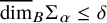 .
.
Proof. (1) Let
$\epsilon _0,\varsigma ,\kappa $
 be the constants in Theorem 5.2. Fix

Let
$h_0>0,M> C>1,\rho \in (0,1)$
 be the constants determined by Theorem 5.2.
Now fix any
$\delta>0$
 . Choose
$h(\delta ,\hat m,\hat M)\in (0,h_0)$
. Choose
$h(\delta ,\hat m,\hat M)\in (0,h_0)$
 such that Lemma 3.7 holds. Choose

Now fix any
$\alpha =[a_1,a_2,\cdots ]$
 such that (5.1) holds. Then for any
$n\ge \hat m+1$
such that (5.1) holds. Then for any
$n\ge \hat m+1$
 , we have

By Theorem 5.2, there exists
$\{I_i: 1\le i\le q_{\hat m}(\alpha )\}$
 and, for any
$1\le i\le q_{\hat m}(\alpha ),$
and, for any
$1\le i\le q_{\hat m}(\alpha ),$
 there exist
$\Omega _\ast ^{(i)}$
there exist
$\Omega _\ast ^{(i)}$
 and
$\mathcal I(\Omega _\ast ^{(i)})$
and
$\mathcal I(\Omega _\ast ^{(i)})$
 such that Theorem 5.2 (2-1) and (2-2) hold. Then by Theorem 4.3(1), we have

(2) By the assumption, for any
$n\ge \hat m+1$
 we also have

Then by Theorem 4.3(2), we have

5.3 Proofs of Theorems 1.4 and 1.3
Given Proposition 5.4, the proofs are essentially the same as those of Theorem 1.1 in [Reference Helffer, Liu, Qu and Zhou42]. The only extra issue is the parity of
$q_{\hat m}(\alpha )$
 . To deal with this, we need the following well-known fact. We also include a very short proof.
Lemma 5.5. Given
$\alpha \in [0,1]\setminus {\mathbb Q}$
 , assume
$p_n(\alpha )/q_n(\alpha )$
, assume
$p_n(\alpha )/q_n(\alpha )$
 is the n-th convergent of
$\alpha $
is the n-th convergent of
$\alpha $
 . Then for any
$n\in {\mathbb N}$
. Then for any
$n\in {\mathbb N}$
 , at least one of
$q_n(\alpha ), q_{n+1}(\alpha )$
, at least one of
$q_n(\alpha ), q_{n+1}(\alpha )$
 is odd.
Proof. By [Reference Khinchin55, Theorem 2],
$q_np_{n-1} - q_{n-1}p_n = (-1)^n$
 . Thus
$q_n$
. Thus
$q_n$
 and
$q_{n-1}$
and
$q_{n-1}$
 are coprime and hence not both even.
Proof of Theorem 1.4.
By Remark 5.1, we only need to show that
$\mathscr F_B(\delta )\cap [0,1]$
 is dense in
$[0,1]$
is dense in
$[0,1]$
 and has positive Hausdorff dimension.
First, we show that
$\mathscr F_B(\delta )\cap [0,1]$
 has positive Hausdorff dimension. Take
$L=L(\delta , 2,2)$
has positive Hausdorff dimension. Take
$L=L(\delta , 2,2)$
 as in Proposition 5.4. Define

Then for any
$\alpha \in \mathscr F$
 , we have
$q_2(\alpha )=3.$
, we have
$q_2(\alpha )=3.$
 By Proposition 5.4, we have
$\overline \dim _B \Sigma _\alpha \le \delta .$
By Proposition 5.4, we have
$\overline \dim _B \Sigma _\alpha \le \delta .$
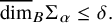 So
$\mathscr F\subset \mathscr F_B(\delta )\cap [0,1]$
So
$\mathscr F\subset \mathscr F_B(\delta )\cap [0,1]$
 . By [Reference Good37, Lemma B.1],
$\dim _H G^2(\mathscr F)>0.$
. By [Reference Good37, Lemma B.1],
$\dim _H G^2(\mathscr F)>0.$
 By a simple computation, we know that
$G^2: \mathscr F\to G^2(\mathscr F)$
By a simple computation, we know that
$G^2: \mathscr F\to G^2(\mathscr F)$
 is a bi-Lipschitz map. So
$\dim _H \mathscr F=\dim _H G^2(\mathscr F)>0$
is a bi-Lipschitz map. So
$\dim _H \mathscr F=\dim _H G^2(\mathscr F)>0$
 . Hence
$\dim _H\mathscr F_B(\delta )\cap [0,1]>0.$
. Hence
$\dim _H\mathscr F_B(\delta )\cap [0,1]>0.$

Next we show that
$\mathscr F_B(\delta )\cap [0,1]$
 is dense in
$[0,1]$
is dense in
$[0,1]$
 . Fix any
$N\ge 2$
. Fix any
$N\ge 2$
 and take

Define
$\mathscr F_N:=\mathscr F_N^o\cup \mathscr F_N^e$
 , where

By Proposition 5.4,
$\mathscr F_N^o\subset \mathscr F_B(\delta )\cap [0,1]$
 . If
$\alpha \in \mathscr F_N^e$
. If
$\alpha \in \mathscr F_N^e$
 , then by Lemma 5.5,
$q_{N+1}(\alpha )$
, then by Lemma 5.5,
$q_{N+1}(\alpha )$
 is odd. Then by Proposition 5.4 again,
$\mathscr F_N^e\subset \mathscr F_B(\delta )\cap [0,1]$
is odd. Then by Proposition 5.4 again,
$\mathscr F_N^e\subset \mathscr F_B(\delta )\cap [0,1]$
 . So
$\mathscr F_N\subset \mathscr F_B(\delta )\cap [0,1]$
. So
$\mathscr F_N\subset \mathscr F_B(\delta )\cap [0,1]$
 . Now define

Then
$\widehat {\mathscr F}\subset \mathscr F_B(\delta )\cap [0,1]$
 and by the same argument as Section 4.4 of [Reference Helffer, Liu, Qu and Zhou42],
$\widehat {\mathscr F}$
and by the same argument as Section 4.4 of [Reference Helffer, Liu, Qu and Zhou42],
$\widehat {\mathscr F}$
 is dense in
$[0,1]$
is dense in
$[0,1]$
 . So
$\mathscr F_B(\delta )\cap [0,1]$
. So
$\mathscr F_B(\delta )\cap [0,1]$
 is also dense in
$[0,1]$
is also dense in
$[0,1]$
 .
.
Proof of Theorem 1.3.
Let
$\mathscr F$
 and
$\widehat {\mathscr F}$
and
$\widehat {\mathscr F}$
 be defined as above. Then
$\widetilde {\mathscr F}:={\mathscr F}\cup \widehat {\mathscr F}$
be defined as above. Then
$\widetilde {\mathscr F}:={\mathscr F}\cup \widehat {\mathscr F}$
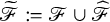 is dense in
$[0,1]$
is dense in
$[0,1]$
 and of positive Hausdorff dimension. For any
$\alpha \in \widetilde {\mathscr F}$
and of positive Hausdorff dimension. For any
$\alpha \in \widetilde {\mathscr F}$
 , we have shown that
$\overline {\dim }_B\Sigma _\alpha \le \delta <1$
, we have shown that
$\overline {\dim }_B\Sigma _\alpha \le \delta <1$
 . Consequently,
$\beta (\alpha )=0$
. Consequently,
$\beta (\alpha )=0$
 by [Reference Jitomirskaya and Zhang50]. By [Reference Helffer, Liu, Qu and Zhou42] Theorem 1.3, we have
$\dim _H \Sigma _\alpha>0.$
by [Reference Jitomirskaya and Zhang50]. By [Reference Helffer, Liu, Qu and Zhou42] Theorem 1.3, we have
$\dim _H \Sigma _\alpha>0.$

A A short reminder on the results in [Reference Helffer and Sjöstrand44]
The following theorem was proved in [Reference Helffer and Sjöstrand44] and is sufficient for the results given in [Reference Helffer, Liu, Qu and Zhou42].
Theorem A.1. Let
$\hat m \in {\mathbb Z}_+$
 and
$M \geq 2$
and
$M \geq 2$
 . There exist
$\eta _0>0$
. There exist
$\eta _0>0$
 and, for
$\eta _1 \in (0,\eta _0 )$
and, for
$\eta _1 \in (0,\eta _0 )$
 , constants
${C=C(\hat m, M,\eta _1)>0}$
, constants
${C=C(\hat m, M,\eta _1)>0}$
 and
$C'=C'(\hat m, M,\eta _1)>0$
and
$C'=C'(\hat m, M,\eta _1)>0$
 such that if

is irrational and satisfies for some
$m\leq \hat m$


then
$\Sigma _{\alpha }$
 is contained in the union of
$q_m(\alpha )$
is contained in the union of
$q_m(\alpha )$
 intervals
$I_\ell (h)$
intervals
$I_\ell (h)$
 (
$\ell =1,\cdots , q_m(\alpha ))$
(
$\ell =1,\cdots , q_m(\alpha ))$
 in the form
$[\gamma _\ell (h), \delta _\ell (h)]$
in the form
$[\gamma _\ell (h), \delta _\ell (h)]$
 with
with

where


For each interval
$I_\ell (h)$
 ,
$\Sigma _{\alpha }\cap I_\ell (h)$
,
$\Sigma _{\alpha }\cap I_\ell (h)$
 can be described as living in a union of closed intervals
$J_j^{(\ell )}$
can be described as living in a union of closed intervals
$J_j^{(\ell )}$
 of length
$\neq 0$
of length
$\neq 0$
 with
$\partial J_{j}^{(\ell )} \subset \Sigma _{\alpha }\,$
with
$\partial J_{j}^{(\ell )} \subset \Sigma _{\alpha }\,$
 ,
$J_{j+1}^{(\ell )}$
,
$J_{j+1}^{(\ell )}$
 on the right of
$J_j^{(\ell )}$
on the right of
$J_j^{(\ell )}$
 and
and


The other bands have size

For
$j\neq 0$
 , if
$\kappa _j^{(\ell )} $
, if
$\kappa _j^{(\ell )} $
 is the affine function sending
$J_j^{(\ell )}$
is the affine function sending
$J_j^{(\ell )}$
 into
$[-2,+2]$
into
$[-2,+2]$
 , then

where the
$J_{j,k}^{(\ell )}$
 have analogous properties to the
$J_j^{(\ell )} $
have analogous properties to the
$J_j^{(\ell )} $
 with
$a_{m+1}$
with
$a_{m+1}$
 replaced by
$a_{m+2}$
replaced by
$a_{m+2}$
 and (A.7) can be improved in the form

One can then iterate indefinitely.
Remark A.2.
$\eta _1$
 corresponds to the exclusion in each interval and at each step of the renormalization of a small interval of size
$\approx 2\eta _1$
corresponds to the exclusion in each interval and at each step of the renormalization of a small interval of size
$\approx 2\eta _1$
 for which another analysis has to be done and which was the object of [Reference Helffer and Sjöstrand45]. This corresponds to the energy
$0$
for which another analysis has to be done and which was the object of [Reference Helffer and Sjöstrand45]. This corresponds to the energy
$0$
 for the map
$(x,\xi ) \mapsto 2( \cos x + \cos \xi $
for the map
$(x,\xi ) \mapsto 2( \cos x + \cos \xi $
 ). This refined analysis was not needed in [Reference Helffer, Liu, Qu and Zhou42].
Remark A.3. The possibility of having
$\delta _\ell =\gamma _{\ell +1}$
 is due to the occurrence of touching bands. van Mouche [Reference van Mouche72] has proven that it occurs only when
$q_m$
is due to the occurrence of touching bands. van Mouche [Reference van Mouche72] has proven that it occurs only when
$q_m$
 is even and for
$\ell = \frac { q_m} {2}$
is even and for
$\ell = \frac { q_m} {2}$
 . These two touching bands lead to the lower bound (A.6) and the weaker estimate in (A.7).
In the next appendix, we will give more precise information on the excluded intervals appearing in the above theorem.
B Extracts of Harper III
We mainly follow the talk of presentation [Reference Helffer and Sjöstrand46], which was announcing [Reference Helffer and Sjöstrand45]. Note that, concerning the first step, the paper of Helffer–Kerdelhue [Reference Helffer and Kerdelhue41] can be useful for more explicit computations.
We warn that in this section,
${\alpha }\in {\mathbb Z}^2$
 denotes an integer vector to match the notation in [Reference Helffer and Sjöstrand45], while the frequency is related to
$h/2\pi $
denotes an integer vector to match the notation in [Reference Helffer and Sjöstrand45], while the frequency is related to
$h/2\pi $
 .
.
B.1 Introduction
As in [Reference Helffer and Sjöstrand43] we are considering the Harper model

together with perturbations of this operator under the condition that

where
$a_j\in \mathbb N$
 ,
$a_j\geq C_0$
,
$a_j\geq C_0$
 . Here
$C_0$
. Here
$C_0$
 is a sufficiently large constant. In [Reference Helffer and Sjöstrand43], as recalled in Appendix A, a partial description of the spectrum of
$P_0$
is a sufficiently large constant. In [Reference Helffer and Sjöstrand43], as recalled in Appendix A, a partial description of the spectrum of
$P_0$
 has been obtained by an infinite procedure of localizations in subintervals associated with affine dilations. Notice that

where
$\tau _h$
 is the translation operator
$(\tau _h u )(x)= u(x-h)\,,$
is the translation operator
$(\tau _h u )(x)= u(x-h)\,,$
 which can also be understood as an h-pseudo-differential operator of symbol
$\cos \xi + \cos x$
which can also be understood as an h-pseudo-differential operator of symbol
$\cos \xi + \cos x$
 . See footnote 4 for the definition.
Unfortunately, each time that an isolated part of the spectrum was localized in a fixed interval, the methods which were developed in [Reference Helffer and Sjöstrand43] do not permit the procedure to continue in a small neighborhood of the middle of this interval. In [Reference Helffer and Sjöstrand44] the results were generalized to the case when
$\frac {h}{2\pi }$
 is “close” to a rational, but this did not solve the previous problem. Hence, the goal of [Reference Helffer and Sjöstrand46, Reference Helffer and Sjöstrand45] was to complete this description. If we associate with
$P_0$
is “close” to a rational, but this did not solve the previous problem. Hence, the goal of [Reference Helffer and Sjöstrand46, Reference Helffer and Sjöstrand45] was to complete this description. If we associate with
$P_0$
 the symbol

then, for
$0 < \mu \leq 2$
 , the surface of real energy
$\mu $
, the surface of real energy
$\mu $
 , that is, the set
$ \{(x,\xi )\in \mathbb R^2| p_0(x,\xi )=\mu \}$
, that is, the set
$ \{(x,\xi )\in \mathbb R^2| p_0(x,\xi )=\mu \}$
 is decomposed as
$\cup _{\alpha \in \mathbb Z^2} U_{\alpha }(\mu )$
is decomposed as
$\cup _{\alpha \in \mathbb Z^2} U_{\alpha }(\mu )$
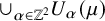 , where
$U_\alpha (\mu )$
, where
$U_\alpha (\mu )$
 is a closed curve surrounding
$2\pi \alpha $
is a closed curve surrounding
$2\pi \alpha $
 for
$0 < \mu < 2$
for
$0 < \mu < 2$
 and which becomes
$\{2\pi \alpha \}$
and which becomes
$\{2\pi \alpha \}$
 for
$\mu =2$
for
$\mu =2$
 . For
$-2 \leq \mu < 0$
. For
$-2 \leq \mu < 0$
 , we have the same type of decomposition (by just replacing
$2\pi \alpha $
, we have the same type of decomposition (by just replacing
$2\pi \alpha $
 by
$2\pi \alpha + (\pi ,\pi )$
by
$2\pi \alpha + (\pi ,\pi )$
 ).
).
Following ideas of Wilkinson, [Reference Helffer and Sjöstrand43] gives a localization of the spectrum of
$P_0$
 in
$[-2,2] \setminus [-\epsilon _0,\epsilon _0]$
in
$[-2,2] \setminus [-\epsilon _0,\epsilon _0]$
 (for small positive
$\epsilon _0$
(for small positive
$\epsilon _0$
 ) in a union of closed intervals of size
$e^{- 1/(C h)}$
) in a union of closed intervals of size
$e^{- 1/(C h)}$
 , which are separated by open intervals of size
$\sim h$
, which are separated by open intervals of size
$\sim h$
 . Each interval corresponds modulo
$\mathcal O(e^{-1/C h})$
. Each interval corresponds modulo
$\mathcal O(e^{-1/C h})$
 to an eigenvalue of a reference problem obtained by “filling” all the “wells”
$U_\alpha $
to an eigenvalue of a reference problem obtained by “filling” all the “wells”
$U_\alpha $
 except one. Analyzing then the tunneling effect between the wells it can be proved that the study of the spectrum in each of these intervals can be reduced to the analysis of the spectrum of an infinite matrix
$W=(w_{\alpha ,\beta })_{(\alpha ,\beta )\in \mathbb Z^2\times {\mathbb Z}^2}$
except one. Analyzing then the tunneling effect between the wells it can be proved that the study of the spectrum in each of these intervals can be reduced to the analysis of the spectrum of an infinite matrix
$W=(w_{\alpha ,\beta })_{(\alpha ,\beta )\in \mathbb Z^2\times {\mathbb Z}^2}$
 , for which the principal contribution can be computed.
Using the symmetry properties of
$w_{\alpha ,\beta }$
 , W is isospectral (up to a multiplicative positive constant) to the
$h'$
, W is isospectral (up to a multiplicative positive constant) to the
$h'$
 -Weyl quantification of some symbol
$p(x,\xi )$
-Weyl quantification of some symbol
$p(x,\xi )$
 which is close to
$p_0$
which is close to
$p_0$
 . Here
$h'\in (0,2\pi ]$
. Here
$h'\in (0,2\pi ]$
 is given by

This implies that

For the spectrum near
$0$
 we do not have a natural localization in wells. Actually, when
$\mu $
we do not have a natural localization in wells. Actually, when
$\mu $
 is close to
$0$
is close to
$0$
 , the energy surface
$p_0=\mu $
, the energy surface
$p_0=\mu $
 is close to the union of the lines

and the difficulty is that
$p_0$
 has critical points at
$(k\pi ,\ell \pi )$
has critical points at
$(k\pi ,\ell \pi )$
 with
$ k + \ell -1\in 2 \mathbb Z$
with
$ k + \ell -1\in 2 \mathbb Z$
 . One is led to analyze the microlocal solutionFootnote
2
of
$(P_0-\mu ) u=0$
. One is led to analyze the microlocal solutionFootnote
2
of
$(P_0-\mu ) u=0$
 near these points.
Let
$s(0,1)$
 be the segment
$[(0,\pi ),(\pi ,0)]$
be the segment
$[(0,\pi ),(\pi ,0)]$
 , and
$s(0,j)=\mathcal H^{1-j}(s(0,1))$
, and
$s(0,j)=\mathcal H^{1-j}(s(0,1))$
 , where

and
$s(\alpha ,j) = s(0,j) + \{ 2\pi \alpha \}$
 . Near the middle of
$s(0,1)$
. Near the middle of
$s(0,1)$
 , the microlocal solution of
$(P_0-\mu )u=0$
, the microlocal solution of
$(P_0-\mu )u=0$
 is unique up to a multiplicative constant. Let us denote by
$u_{0,1}$
is unique up to a multiplicative constant. Let us denote by
$u_{0,1}$
 such a solution. Using the symmetries of
$P_0$
such a solution. Using the symmetries of
$P_0$
 , we can define
$u_{\alpha ,j}$
, we can define
$u_{\alpha ,j}$
 as a microlocal solution near
$s(\alpha ,j)$
as a microlocal solution near
$s(\alpha ,j)$
 . Near a branching point (say, for example,
$(0,\pi )$
. Near a branching point (say, for example,
$(0,\pi )$
 ) the microlocal kernel of
$(P_0-\mu )$
) the microlocal kernel of
$(P_0-\mu )$
 has dimension
$2$
has dimension
$2$
 and an element of the kernel can be written as

Here the parameters are
$(x_1,x_3)$
 and
$(y_2,y_4)$
and
$(y_2,y_4)$
 is then determined by

where U is a
$\mu $
 -dependent unitary matrix whose behavior can be analyzed asymptotically. Now we choose a suitable family
$\{f_{\alpha ,j}\}$
-dependent unitary matrix whose behavior can be analyzed asymptotically. Now we choose a suitable family
$\{f_{\alpha ,j}\}$
 of
$L^2$
of
$L^2$
 functions, such that
$f_{\alpha ,j}$
functions, such that
$f_{\alpha ,j}$
 is microlocalized in the middle of
$s(\alpha ,j)$
is microlocalized in the middle of
$s(\alpha ,j)$
 and such that
$\langle u_{\alpha ,j}|f_{\alpha ,j}\rangle =1$
and such that
$\langle u_{\alpha ,j}|f_{\alpha ,j}\rangle =1$
 . Then one introduces what is called in other contexts a Grushin problem. By introduction of

One obtains a bijective operator

from
$L^2(\mathbb R)\times \ell ^2(\mathbb Z^2;\mathbb C^2_p)$
 onto
$L^2(\mathbb R)\times \ell ^2(\mathbb Z^2;\mathbb C^2_i)$
onto
$L^2(\mathbb R)\times \ell ^2(\mathbb Z^2;\mathbb C^2_i)$
 , where
$\mathbb C^2_i$
, where
$\mathbb C^2_i$
 and
$\mathbb C^2_p$
and
$\mathbb C^2_p$
 are copies of
$\mathbb C^2$
are copies of
$\mathbb C^2$
 indexed respectively by
$1,3$
indexed respectively by
$1,3$
 and
$2,4$
and
$2,4$
 .
.
If the inverse is denoted by
$\left (\begin {array}{cc} E&E_+\\E_-&E_{-+}\end {array}\right )$
 , then
$\mu \in Sp(P_0)$
, then
$\mu \in Sp(P_0)$
 if and only if
$0\in Sp(E_{-+}(\mu ))$
if and only if
$0\in Sp(E_{-+}(\mu ))$
 . As with W, one can see
$E_{-+}$
. As with W, one can see
$E_{-+}$
 as an infinite matrix
$(E_{-+}(\alpha ,\beta ))$
as an infinite matrix
$(E_{-+}(\alpha ,\beta ))$
 where
$E_{-+}(\alpha ,\beta )$
where
$E_{-+}(\alpha ,\beta )$
 is now a
$2\times 2$
is now a
$2\times 2$
 matrix. It can be shown that
$0\in Sp(E_{-+})$
matrix. It can be shown that
$0\in Sp(E_{-+})$
 if and only if
$0\in Sp (P)$
if and only if
$0\in Sp (P)$
 , where P is the
$h'$
, where P is the
$h'$
 -quantification of a matrix-valued symbol.
Fortunately, the analysis of these
$2\times 2$
 systems is rather similar to the analysis of perturbed Harper models, and rather often, one can indeed reduce the analysis to the scalar case. Nevertheless note that the linear dependence of the spectral parameter is lost and that P is no more selfadjoint. But it can be found
$h'$
systems is rather similar to the analysis of perturbed Harper models, and rather often, one can indeed reduce the analysis to the scalar case. Nevertheless note that the linear dependence of the spectral parameter is lost and that P is no more selfadjoint. But it can be found
$h'$
 -pseudodifferential operators
$P_1,P_2$
-pseudodifferential operators
$P_1,P_2$
 , which are elliptic near the characteristic set of P, such that
$P_1^*P$
, which are elliptic near the characteristic set of P, such that
$P_1^*P$
 and
$P P_2^*$
and
$P P_2^*$
 are selfadjoint.
B.2 Main results
For
$h>0$
 we introduce the following operators initially defined on
$\mathcal S(\mathbb R)$
we introduce the following operators initially defined on
$\mathcal S(\mathbb R)$
 :
:
-
1. $ \mathcal F_h u (\xi ) := \frac {1}{2\pi h} \int e^{-i\xi /h} u(x)\, dx$
. -
2. $ \tau _1u(x)= u(x-2\pi )$
,
$\tau _2 u (x)= e^{2i\pi / h} u(x)$
. -
3. $T_\alpha =\tau _1^{\alpha _1} \tau _2^{\alpha _2}$
for
$\alpha \in \mathbb Z^2$
.



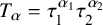

We denote by V the antilinear quantification of the antisymplectic reflection
$(x,\xi ) \mapsto \mathfrak S (x,\xi )= (\xi ,x)$
 . Note that
$V^2=I$
. Note that
$V^2=I$
 . and that

where
$ U_t = e^{it ((hD)^2+x^2-h)/h}$
 and
$\Gamma $
and
$\Gamma $
 is the complex conjugation.
In the iteration (“renormalization”) procedure we will meet two types of operators.
Definition B.1. We say that the triple
$(P,P_1,P_2)$
 of h-pseudodifferential operators is of type
$1$
of h-pseudodifferential operators is of type
$1$
 if
$P_1^*P$
if
$P_1^*P$
 and
$P P_2^*$
and
$P P_2^*$
 are selfadjoint and
-
1. $[P,T_\alpha ]=0\,,\, [P_j, T_\alpha ]=0\,,\, \forall \alpha \in \mathbb Z^2\,,$
-
2. $[P,V]=0\,,\, [P_j,V]=0\,,$
-
3. $P \mathcal F =\mathcal F P^*$
,
$P_1 \mathcal F =\mathcal F P_2^*$
,
$P_2 \mathcal F =\mathcal F P_1^*$
.




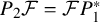
This is an extension of the notion of invariant self-adjoint operators which corresponds to the case
$P_1=I$
 and
$P_2=I$
and
$P_2=I$
 .
.
Definition B.2. We say that the triple
$(P,P_1,P_2)$
 of h-pseudodifferential operators depending on a complex parameter
$\mu $
of h-pseudodifferential operators depending on a complex parameter
$\mu $
 with
$|\mu | < 4$
with
$|\mu | < 4$
 is of typeFootnote
3
$\textbf {1f}$
is of typeFootnote
3
$\textbf {1f}$
 if it is of type
$1$
if it is of type
$1$
 for
$\mu $
for
$\mu $
 -real and if there exists
$\epsilon>0$
-real and if there exists
$\epsilon>0$
 such that the associated Weyl symbolsFootnote
4
$p(\mu ,x,\xi )$
such that the associated Weyl symbolsFootnote
4
$p(\mu ,x,\xi )$
 ,
$p_j(\mu ,x,\xi )$
,
$p_j(\mu ,x,\xi )$
 are holomorphic in
$\mu ,x,\xi $
are holomorphic in
$\mu ,x,\xi $
 for
$|\mu | <4$
for
$|\mu | <4$
 ,
$|\Im (x,\xi )| < \frac 1 \epsilon $
,
$|\Im (x,\xi )| < \frac 1 \epsilon $
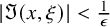 and satisfy there

Note that the Harper model (whose symbol is
$\cos \xi + \cos x$
 ) which is the first operator in the iteration procedure, is of this type.
In this context we can define
$\epsilon (P)=\epsilon (P,P_1,P_2)$
 as the infimum over the
$\epsilon>0$
as the infimum over the
$\epsilon>0$
 such that the above holds.
Definition B.3. We say that the triple
$(P,P_1,P_2)$
 of
$2\times 2$
of
$2\times 2$
 matrix-valued h-pseudodifferential operators
$L^2(\mathbb R;\mathbb C_i^2)\mapsto L^2(\mathbb R;\mathbb C_p^2)$
matrix-valued h-pseudodifferential operators
$L^2(\mathbb R;\mathbb C_i^2)\mapsto L^2(\mathbb R;\mathbb C_p^2)$
 is of type
$2$
is of type
$2$
 if
$P_1^* P$
if
$P_1^* P$
 and
$P P_2^*$
and
$P P_2^*$
 are selfadjoint and
-
1. $[P,T_\alpha ]=0\,,\, [P_j, T_\alpha ]=0\,,\, \forall \alpha \in \mathbb Z^2\,,$
-
2. $VP= PV T^2 $
,
$VP_j= P_jVT^2\,,$
-
3. $P \mathcal F T=\mathcal F T P^*$
,
$P_1 \mathcal F T=\mathcal F T P_2^*$
,
$P_2 \mathcal FT =\mathcal F T P_1^*$
.


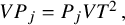



Definition B.4. We say that the triple
$(P,P_1,P_2)$
 of
$2\times 2$
of
$2\times 2$
 matrix-valued h-pseudodifferential operators depending on a complex parameter
$\mu $
matrix-valued h-pseudodifferential operators depending on a complex parameter
$\mu $
 with
$|\mu | < 4$
with
$|\mu | < 4$
 is of type
$\textbf {2f}$
is of type
$\textbf {2f}$
 if it is of type
$2$
if it is of type
$2$
 for
$\mu $
for
$\mu $
 -real and if there exists
$\epsilon>0$
-real and if there exists
$\epsilon>0$
 such that the associated Weyl symbols
$p(\mu ,x,\xi )$
such that the associated Weyl symbols
$p(\mu ,x,\xi )$
 ,
$p_j(\mu ,x,\xi )$
,
$p_j(\mu ,x,\xi )$
 are holomorphic in
$\mu ,x,\xi $
are holomorphic in
$\mu ,x,\xi $
 for
$|\mu | <4$
for
$|\mu | <4$
 ,
$|\Im (x,\xi )| < \frac 1 \epsilon $
,
$|\Im (x,\xi )| < \frac 1 \epsilon $
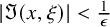 and satisfy there

Here

where
$a,b\neq 0$
 depend holomorphically on
$\mu $
depend holomorphically on
$\mu $
 ,
,

where the
$\beta _j$
 are holomorphic,
$|\beta _j|\leq \epsilon $
are holomorphic,
$|\beta _j|\leq \epsilon $
 ,
$\beta _j$
,
$\beta _j$
 is real for
$\mu $
is real for
$\mu $
 real.
real.
Moreover, for
$\mu \in \mathbb R$


In this context we can define
$\epsilon (P)=\epsilon (P,P_1,P_2)$
 as the infimum over the
$\epsilon>0$
as the infimum over the
$\epsilon>0$
 such that the above holds and

For
$\mu $
 real, we get with the help of (B.4),

As
$\frac {i}{b\bar a}$
 is real, this is a good indication that the operators of type
$\textbf {2f}$
is real, this is a good indication that the operators of type
$\textbf {2f}$
 should behave like the operators of type
$\textbf {1f}$
should behave like the operators of type
$\textbf {1f}$
 . To be shorter we say that P is of type
$ \textbf {1f}$
. To be shorter we say that P is of type
$ \textbf {1f}$
 (or
$\textbf {2f}$
(or
$\textbf {2f}$
 ) if there exist
$P_1,P_2$
) if there exist
$P_1,P_2$
 s.t. the corresponding triple
$(P,P_1,P_2)$
s.t. the corresponding triple
$(P,P_1,P_2)$
 is of type
$\textbf {1f}$
is of type
$\textbf {1f}$
 (or
$\textbf {2f}$
(or
$\textbf {2f}$
 ).
).
Finally, we define the
$\mu $
 -spectrum of
$P(\mu ) $
-spectrum of
$P(\mu ) $
 and denote it by
$\mu -Sp(P)$
and denote it by
$\mu -Sp(P)$
 as the following set:

Of course, if
$P(\mu )= P-\mu $
 , we recover the usual notion of spectrum of P.
Theorem B.5. There exist
$\epsilon _0>0$
 and functions
$F: (0,1]\mapsto [1,+\infty )$
and functions
$F: (0,1]\mapsto [1,+\infty )$
 ,
$h_0: (0,1]\mapsto (0,1]$
,
$h_0: (0,1]\mapsto (0,1]$
 ,
$\alpha : (0,1]^2 \mapsto (0,1]$
,
$\alpha : (0,1]^2 \mapsto (0,1]$
 with
$\alpha (\epsilon ,h)$
with
$\alpha (\epsilon ,h)$
 tending to zero as h tends to zero, such that if
$\epsilon \in (0,1]$
tending to zero as h tends to zero, such that if
$\epsilon \in (0,1]$
 and if P is of type
$\textbf {1f}$
and if P is of type
$\textbf {1f}$
 with
$\epsilon (P)\leq \epsilon _0$
with
$\epsilon (P)\leq \epsilon _0$
 ,
$0 < h \leq h_0(\epsilon )$
,
$0 < h \leq h_0(\epsilon )$
 , then

where the
$ J_j$
 are disjoint closed intervals (placed in increasing order) such that, for each j, there exists a real affine map
$\mathcal H_j: \mu \mapsto \mu '$
are disjoint closed intervals (placed in increasing order) such that, for each j, there exists a real affine map
$\mathcal H_j: \mu \mapsto \mu '$
 , such that:
-
1. For $j\neq 0$
, $$ \begin{align*}\mathcal H_j( J_j \cap \mu-Sp(P))=\mu'-Sp(Q)\end{align*} $$where Q is an operator of type $\mathbf {1f}$
with
$(\mu ,h)$
replaced by
$(\mu ',h')$
and with
$\epsilon (Q) \leq \epsilon $
.
-
2.
$$ \begin{align*}\mathcal H_0(J_0 \cap \,\mu-Sp(P))= \mu'-Sp(Q)\,,\end{align*} $$where, for each $\mu ^{\prime }_0\in \mathcal H_0( J_0)$
, Q is an operator of type
$\mathbf {2f}$
with
$(\mu ,h)$
replaced by
$(\mu '',h')$
, where
$\mu '=\mu ^{\prime }_0 + \mu ''$
, and with $$ \begin{align*}\epsilon (Q)\leq \alpha (\epsilon,h)\,,\, C(Q)\leq F(\epsilon)\,.\end{align*} $$For each fixed $\epsilon>0$
, the width of
$J_0$
satisfies $$ \begin{align*}\frac 1C h \leq |J_0| \leq Ch\end{align*} $$and
$$ \begin{align*}\frac 1C \frac{\log(\frac 1h)}{h}\leq \frac{d \mathcal H_0}{d\mu} \leq C \frac{\log(\frac 1h)}{h}\,. \end{align*} $$
The length of $J_j$
for
$j\neq 0$
is in
$[\frac 1C e^{-1/Ch}, C \frac {h} {\log (\frac 1h)}]$
and the separation between
$ J_j$
and
$ J_{j+1}$
belongs to
$[\frac {h}{C\log (\frac 1h)}, Ch]$
.


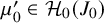


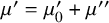


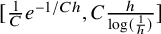


We denote the gaps between the intervals by
$ \{ G_i: i\ne 0\}. $
 We denote the center of
$J_i$
We denote the center of
$J_i$
 by
$c_i$
by
$c_i$
 and the center of
$G_i$
and the center of
$G_i$
 by
$g_i$
by
$g_i$
 . Then, based on our previous discussion, we summarize the results related to the lengths of bands and gaps appearing in Theorem B.5 as follows (assume
$h\sim 1/a_n$
. Then, based on our previous discussion, we summarize the results related to the lengths of bands and gaps appearing in Theorem B.5 as follows (assume
$h\sim 1/a_n$
 ):
):
Proposition B.6. Assume the hypotheses of Theorem B.5
Footnote
5
. Then there exist
$\eta _0>0$
 and, for any
$\eta _1\in (0,\eta _0]$
and, for any
$\eta _1\in (0,\eta _0]$
 ,
$h_0>0$
,
$h_0>0$
 ,
$\hat C>1$
,
$\hat C>1$
 and
$M>0$
and
$M>0$
 such that, if
$0 < h \leq h_0$
such that, if
$0 < h \leq h_0$
 , one has with
$\hat c =\frac {1}{\hat C}$
, one has with
$\hat c =\frac {1}{\hat C}$
 ,
,
1) If
$J_i, G_j\subset [-4,-\eta _1 ]\cup [\eta _1 ,4]$
 , then

Moreover

2) If
$J_i, G_j\subset [-Mh,Mh]$
 and
$i\ne 0$
and
$i\ne 0$
 , then

Moreover

3) If
$J_i, G_j\subset [-\eta _1 ,-Mh]\cup [M h,\eta _1 ]$
 , thenFootnote
6
, thenFootnote
6

Theorem B.7. There exist functions
$\tilde \epsilon _0: [1,\infty )\mapsto (0,1]$
 ,
$F: (0,1]\mapsto [1,+\infty )$
,
$F: (0,1]\mapsto [1,+\infty )$
 ,
$\tilde h_0: (0,1]\times [1,\infty )\mapsto (0,1]$
,
$\tilde h_0: (0,1]\times [1,\infty )\mapsto (0,1]$
 ,
$\tilde \alpha : (0,1]\times [1,\infty )\times (0,1]\mapsto (0,1]$
,
$\tilde \alpha : (0,1]\times [1,\infty )\times (0,1]\mapsto (0,1]$
 with
$\tilde \alpha (\epsilon ,C,h)$
with
$\tilde \alpha (\epsilon ,C,h)$
 tending to
$0$
tending to
$0$
 as
$h\rightarrow 0$
as
$h\rightarrow 0$
 for fixed
$(\epsilon , C)$
for fixed
$(\epsilon , C)$
 , s.t. if
$0< \epsilon \leq 1$
, s.t. if
$0< \epsilon \leq 1$
 ,
$C\geq 1$
,
$C\geq 1$
 and P is of type
$\textbf {2f}$
and P is of type
$\textbf {2f}$
 with
$C(P) \leq C$
with
$C(P) \leq C$
 ,
$\epsilon (P)\leq \tilde \epsilon _0(C)$
,
$\epsilon (P)\leq \tilde \epsilon _0(C)$
 ,
$0 < h < \tilde h_0(\epsilon ,C))$
,
$0 < h < \tilde h_0(\epsilon ,C))$
 , then

where the
$J_j$
 are closed disjoint intervals (placed in increasing order), and for each j there exists an affine application
$\mathcal H_j:\mu \mapsto \mu '$
are closed disjoint intervals (placed in increasing order), and for each j there exists an affine application
$\mathcal H_j:\mu \mapsto \mu '$
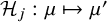 such that we have either
$(a)$
such that we have either
$(a)$
 or
$(b)$
or
$(b)$
 (with the same change of parameters as in the previous theorem):
-
(a)
$$ \begin{align*}\mathcal H_j(J_j \cap \mu-Sp(P))=\mu'-Sp(Q)\end{align*} $$where Q is an operator of type $\textbf {1f}$
with
$\epsilon (Q) \leq \epsilon $
.
-
(b)
$$ \begin{align*}\mathcal H_j(J_j \cap \,\mu-Sp(P))= \mu'-Sp(Q)\,,\end{align*} $$where Q is an operator of type $\textbf {2f}$
with $$ \begin{align*}\epsilon (Q)\leq \tilde \alpha (\epsilon,C, h)\,,\, C(Q)\leq F(\epsilon)\,.\end{align*} $$


For each fixed
$(\epsilon ,C)$
 there exists
$E>1$
there exists
$E>1$
 such that:
-
○ In case (b) the width of $J_j$
satisfies $$ \begin{align*}0 < \frac 1E h \leq | J_j| \leq E h \end{align*} $$and
$$ \begin{align*}0 < \frac 1E \frac{\log(\frac 1h)}{h} \leq \frac{d \mathcal H_j}{d\mu} \leq E \frac{\log(\frac 1h)}{h}\,. \end{align*} $$
-
○ In case (a), the width of $J_j$
belongs to
$[\frac 1{E} e^{-E/h}, E \frac {h} {\log (\frac 1h)}]$
and the separation between
$J_j$
and
$J_{j+1}$
belongs to
$[\frac {h}{E\log (\frac 1h)},Eh]$
.The separation between two intervals of type (b) is larger than $\frac {1}{E}$
.


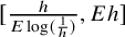

There are essentially no differences in the statements. Here are the small differences:
-
○ We have a finite number of “critical values”. In the (1f) case, we only had one close to zero. The last statement of the theorem gives a uniform bound for the intervals of type (b). The theorem also gives that the different intervals of type (b) have uniformly comparable size.
-
○ For each of these critical values, we have an interval of type (b).
-
○ Outside the h-neighborhoods of these “critical values” which are determined by $\sin (2 \arg b(\mu ))\sim 0$
(see (B.5) and the explanations around) the statements for type (a) intervals are identical to the (1f) statement. We only have to replace the
$c_i$
by the distance of the middle to the critical values.


Let
$\epsilon _0>0$
 as in Theorem B.5 and let

small enough so that if
$h\in (0,h_1]$
 , we have

(note that we can take the same F in the two statements). Let P be an h-pseudo-differential operator with
$0<h \leq h_1$
 satisfying one of the assumptions
$(I)$
satisfying one of the assumptions
$(I)$
 or
$(II)$
or
$(II)$

-
(I) P is of type $\textbf {1f}$
with
$\epsilon (P)\leq \epsilon _0$
, -
(II) P is of type $\textbf {2f}$
with
$\epsilon (P) \leq \tilde \epsilon _0(F(\epsilon _0))$
,
$C(P) \leq F(\epsilon _0)$
.




Then according to the above theorems, the
$\mu $
 -spectrum is localized in the union of closed disjoint intervals and the analysis of the
$\mu $
-spectrum is localized in the union of closed disjoint intervals and the analysis of the
$\mu $
 -spectrum in each interval can be reduced, after an affine transformation
$\mu \mapsto \mu '$
-spectrum in each interval can be reduced, after an affine transformation
$\mu \mapsto \mu '$
 to the analysis of the
$\mu '$
to the analysis of the
$\mu '$
 -spectrum of Q, where Q is an
$h'$
-spectrum of Q, where Q is an
$h'$
 -pseudodifferential operator (with
$h'$
-pseudodifferential operator (with
$h'$
 satisfying (B.3)) satisfying either
$(I)$
satisfying (B.3)) satisfying either
$(I)$
 or
$(II)$
or
$(II)$
 . If
$0 <h' \leq h_1$
. If
$0 <h' \leq h_1$
 , we can then iterate. Taking into account the length of the intervals and their separation, we get
Corollary B.8. There exist
$\epsilon _0>0$
 ,
$C_0>0$
,
$C_0>0$
 such that if

and if P is an h-pseudodifferential operator of type
$\textbf {1f}$
 , with
$\epsilon (P) \leq \epsilon _0$
, with
$\epsilon (P) \leq \epsilon _0$
 , then
$\mu -Sp(P)$
, then
$\mu -Sp(P)$
 has measure
$0$
has measure
$0$
 and its complement is dense in
$\mathbb R$
and its complement is dense in
$\mathbb R$
 .
.
C A slight extension
In [Reference Helffer and Sjöstrand45] we have solved the question of the excluded middle interval appearing in [Reference Helffer and Sjöstrand43] but we were only considering irrational
$\alpha $
 sufficiently close to
$0$
sufficiently close to
$0$
 . We show in this appendix how one should proceed when starting from an irrational sufficiently close to a rational
$\frac pq$
. We show in this appendix how one should proceed when starting from an irrational sufficiently close to a rational
$\frac pq$
 .
.
The question is then to treat the middle interval at each step in order to have the same conclusion obtained in [Reference Helffer and Sjöstrand45] under the stronger condition that
$\hat m =0$
 . This extension is announced at the end of the introduction of [Reference Helffer and Sjöstrand45] in the following way:
In [Reference Helffer and Sjöstrand44], the results of [Reference Helffer and Sjöstrand43] were extended to the case in which, for some N, we have
${|a_j| \geq C_N(a_1,..., a_N,\epsilon _0)}$
 for
$j\geq N+1$
for
$j\geq N+1$
 , but still with the same incompleteness as in [Reference Helffer and Sjöstrand43]. We believe that the techniques in the present paper rather automatically lead to a more complete Cantor structure result also in that case.
The aim of this appendix is to give a few more details about what was meant by “automatically”. We recall that in the case considered in [Reference Helffer and Sjöstrand45] we were starting from
$ \cos x+\cos hD_x $
 and that in [Reference Helffer and Sjöstrand44], given some rational
$\frac p q =[a_1,\cdots , a_m]$
and that in [Reference Helffer and Sjöstrand44], given some rational
$\frac p q =[a_1,\cdots , a_m]$
 we were starting from
$M_{p,q} (x,hD_x)$
we were starting from
$M_{p,q} (x,hD_x)$
 where
$M_{p,q}(x,\xi )$
where
$M_{p,q}(x,\xi )$
 was a
$q \times q$
was a
$q \times q$
 matrix with nice properties. In particular the spectrum consists of q bands, with at most two of them touching in the middle defined as the image of q eigenvalues
$\lambda _\ell (x,\xi ,p,q)$
matrix with nice properties. In particular the spectrum consists of q bands, with at most two of them touching in the middle defined as the image of q eigenvalues
$\lambda _\ell (x,\xi ,p,q)$
 . It has been proven by van Mouche [Reference van Mouche72] that there are no touching bands when q is odd. Each of them has a unique critical value (in its middle)
$\mu _\ell (p,q)$
. It has been proven by van Mouche [Reference van Mouche72] that there are no touching bands when q is odd. Each of them has a unique critical value (in its middle)
$\mu _\ell (p,q)$
 with saddle point structure. In [Reference Helffer and Sjöstrand44] (see Proposition 5.4.1 and the reminder in Appendix A), we show that outside arbitrarily small neighborhoods
$(\gamma _\ell -\epsilon _\ell ,\gamma _\ell +\epsilon _\ell )$
with saddle point structure. In [Reference Helffer and Sjöstrand44] (see Proposition 5.4.1 and the reminder in Appendix A), we show that outside arbitrarily small neighborhoods
$(\gamma _\ell -\epsilon _\ell ,\gamma _\ell +\epsilon _\ell )$
 the spectrum is contained in a union of intervals for which the spectrum is an
$h'$
the spectrum is contained in a union of intervals for which the spectrum is an
$h'$
 -operator of type 1f.
What remains is to get the conclusion of Proposition 4.4 in [Reference Helffer and Sjöstrand45] in
$(\gamma _\ell -\epsilon _\ell ,\gamma _\ell +\epsilon _\ell )$
 starting from
$M_{p,q} (x,hD_x)$
starting from
$M_{p,q} (x,hD_x)$
 instead of a general operator of type 1f.
Once this is proven, the proof is identical since we are now working either with type 1 or type 2 operators. The main remark is that for this proposition we do not need the holomorphic extension in
$|\Im (x,\xi )| < 1/\epsilon $
 but only (by choosing
$\epsilon _\ell $
but only (by choosing
$\epsilon _\ell $
 small enough) the analyticity in a small neighborhood of the saddle point together with the symmetries with respect to
$(x,\xi )\mapsto (-\xi ,x)$
small enough) the analyticity in a small neighborhood of the saddle point together with the symmetries with respect to
$(x,\xi )\mapsto (-\xi ,x)$
 and
$(x,\xi )\mapsto (x,-\xi )$
and
$(x,\xi )\mapsto (x,-\xi )$
 . Once this is observed, we can find in [Reference Helffer and Sjöstrand44] the statement that there exists an analytic function
$f(t) = f_0(t)+ h f_1(t)$
. Once this is observed, we can find in [Reference Helffer and Sjöstrand44] the statement that there exists an analytic function
$f(t) = f_0(t)+ h f_1(t)$
 such that the symbol of
$f(M_{p,q}(x,hD_x),h)$
such that the symbol of
$f(M_{p,q}(x,hD_x),h)$
 can be diagonalized by block modulo an exponentially small contribution and the
$\ell $
can be diagonalized by block modulo an exponentially small contribution and the
$\ell $
 -th eigenvalue is close to
$\cos q\xi + \cos qx $
-th eigenvalue is close to
$\cos q\xi + \cos qx $
 . Here the main point is that

a formula due to Chambers [Reference Chambers19]. This implies

Remark C.1. We observe that what we get, after a diagonalization (modulo exponentially small terms), is a reduction to a h-perturbation of

Note that this operator is unitarily equivalent to

Hence at the price of a change of initial semiclassical parameter, we are in the situation considered in [Reference Helffer and Sjöstrand43, Reference Helffer and Sjöstrand44].
Once proven, the variant of Proposition 4.4, the results from Sections 5 and 6 in [Reference Helffer and Sjöstrand45] only use the conclusion of this proposition. So the only difference is that we have to consider q (instead of
$1$
 ) critical values corresponding to the saddle points of the
$\lambda _{\ell ,p,q} (x,\xi )$
) critical values corresponding to the saddle points of the
$\lambda _{\ell ,p,q} (x,\xi )$
 (
$\ell =1,\cdots ,q$
(
$\ell =1,\cdots ,q$
 ).
).
We insist on the fact that this is only at the first step that we have a (small) difference in the description of the spectrum.
Acknowledgments
The authors would like to thank the referees for many valuable suggestions.
Competing interests
The authors have no competing interests to declare.
Funding support
Y.-H. Qu was supported by the NSFC grant (12371090, 12571097). Q.-H. Liu was supported by NSFC grant (11871098, 12571095). Q. Zhou was supported by NSFC grant (12531006, 12526201) and Nankai Zhide Foundation.


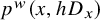


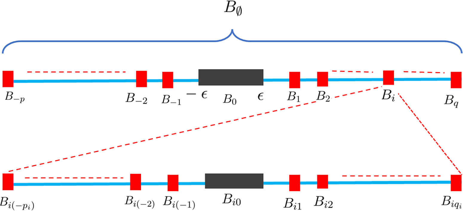


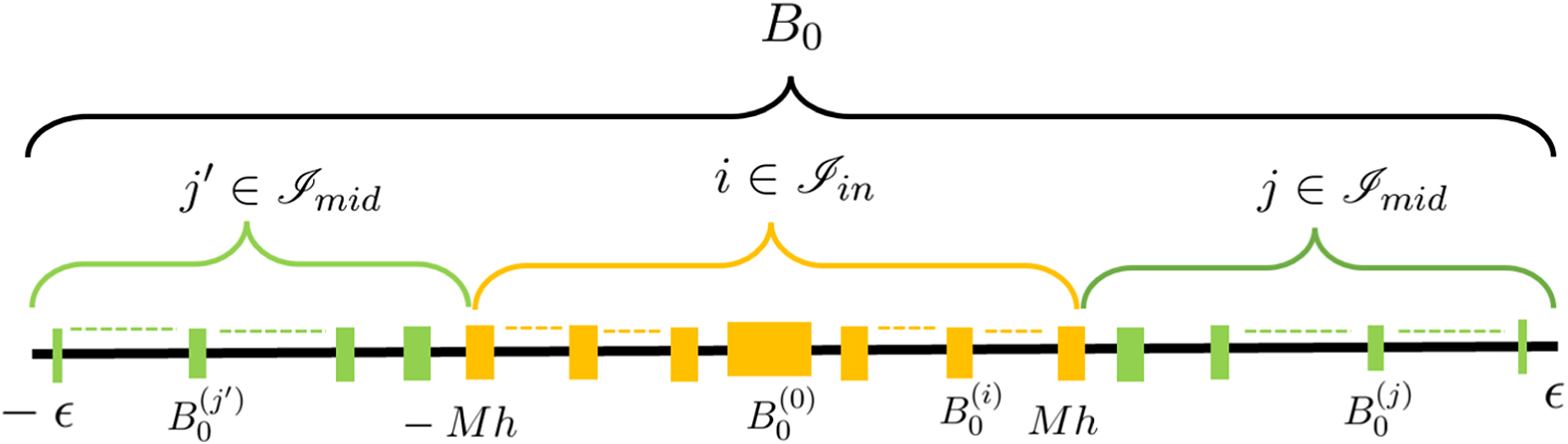

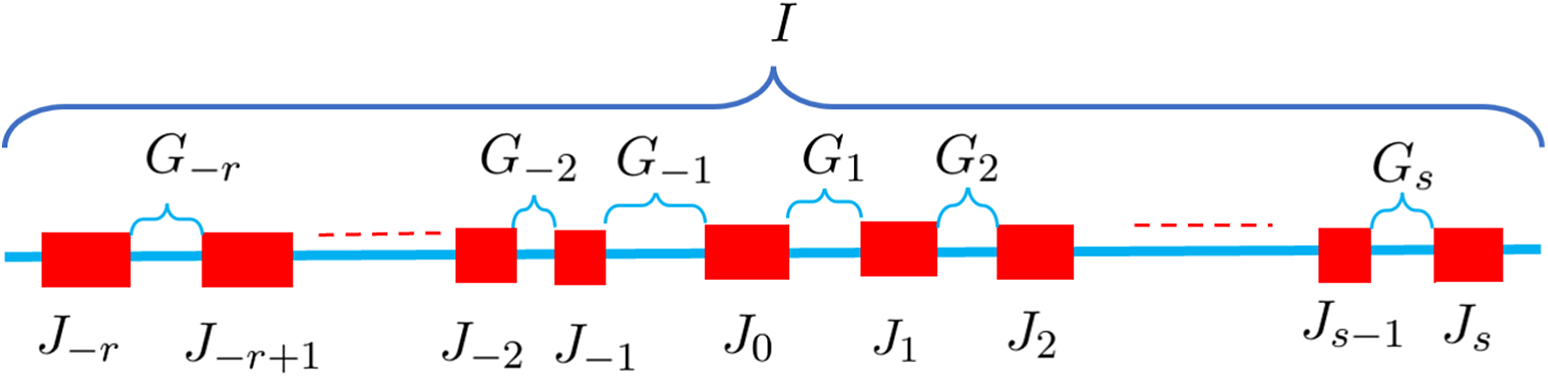

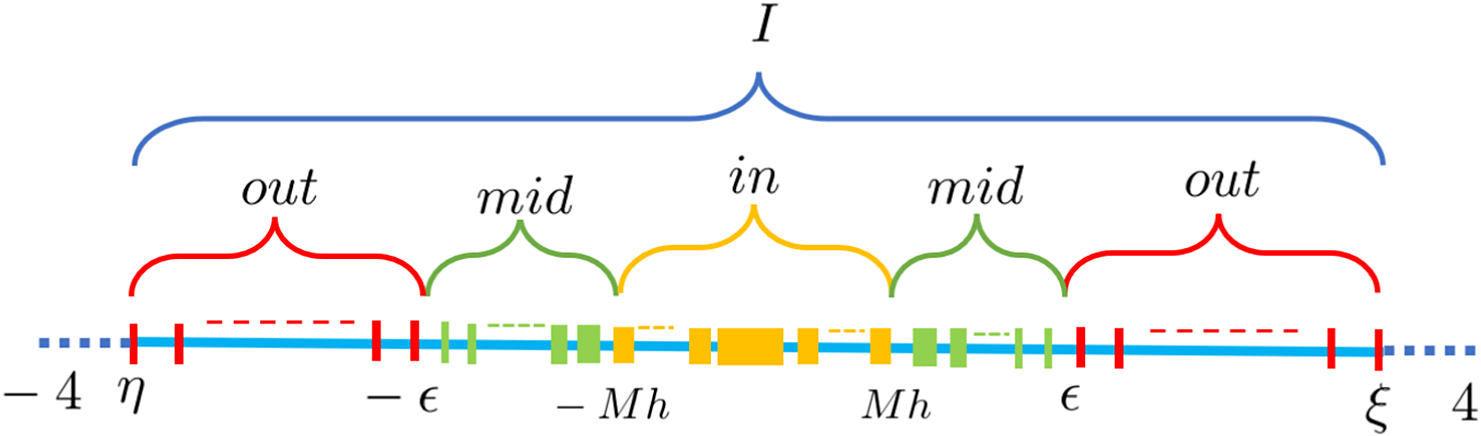
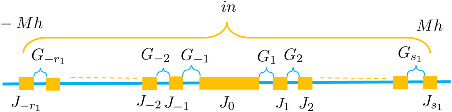
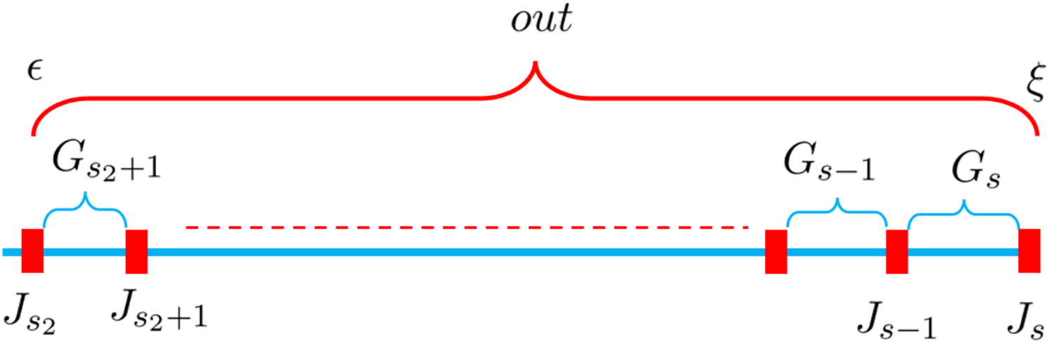

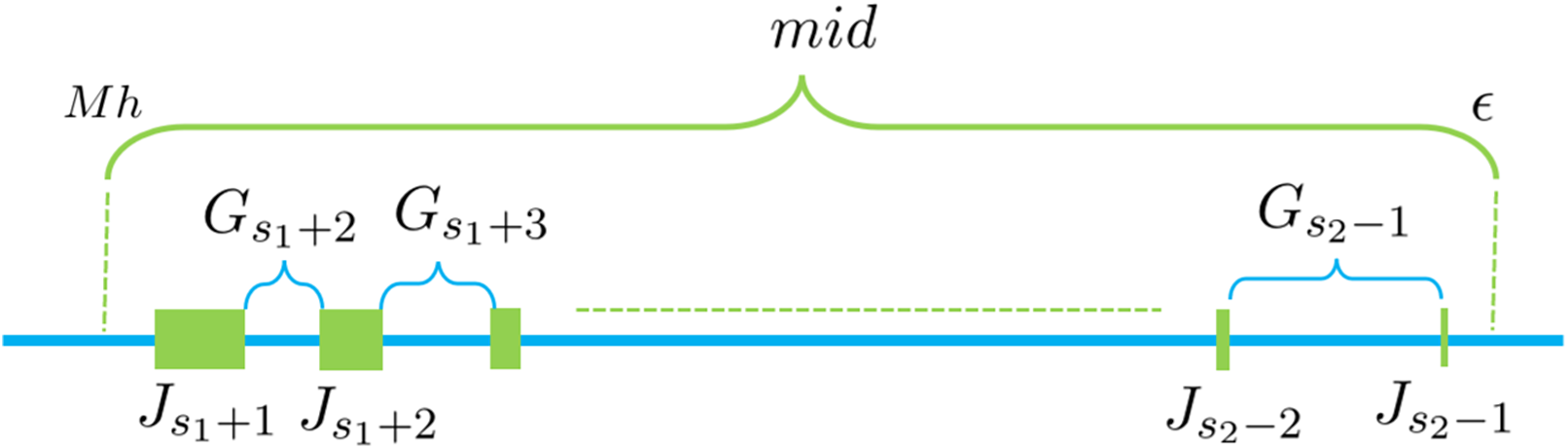
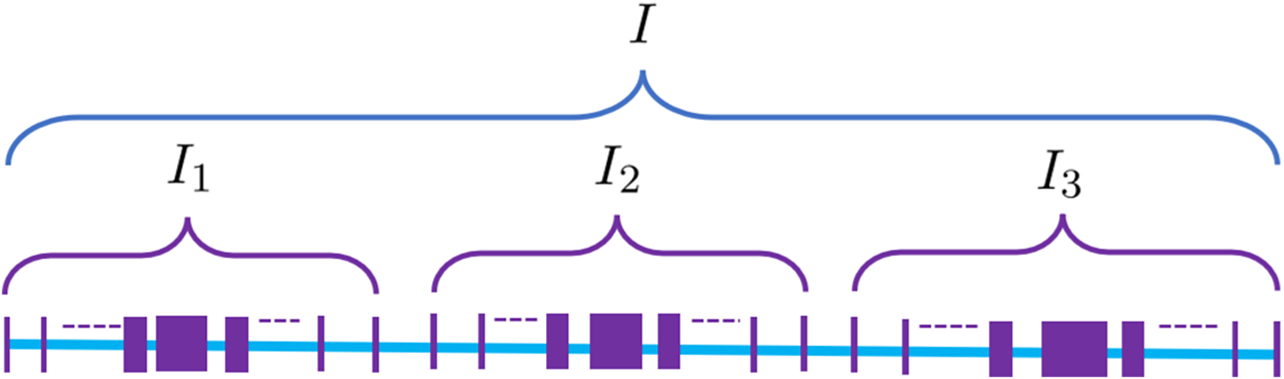


 Open access

