2.1 Ice flow

We consider a steady-state marine ice sheet flowing in the x-direction in a channel of constant width W (Fig. 1). At the grounding line, x = x _g, the ice sheet starts to float, forming an ice shelf of length L _s which terminates at the calving front x = x _c. We use a vertically and laterally integrated flow model of an ice-stream/ice-shelf system. This model has been widely used in the glaciological literature, e.g. Morland (Reference Morland, Van der Veen and Oerlemans1987); MacAyeal (Reference MacAyeal1989); Dupont and Alley (Reference Dupont and Alley2005); Pattyn and others (Reference Pattyn, Huyghe, De Brabander and De Smedt2006); Nick and others (Reference Nick, Vieli, Howat and Joughin2009); Hindmarsh (Reference Hindmarsh2012); Pegler (Reference Pegler2016):

(1a)$$\eqalign{0 = & {\kern 1pt} 2\displaystyle{\partial \over {\partial x}}\left( {A^{ - 1/n}h{\left \vert {\displaystyle{{\partial u} \over {\partial x}}} \right \vert} ^{1/n - 1}\displaystyle{{\partial u} \over {\partial x}}} \right) - \Lambda h \vert u \vert ^{\,p - 1}u - C \vert u \vert ^{m - 1}u \cr & - \rho gh\displaystyle{{\partial (h + b)} \over {\partial x}},\quad {\rm if}\;0 \le x \le x_{\rm g},{\kern 1pt} h \ge \displaystyle{{\rho _{\rm w}} \over \rho} b,} $$

(1b)$$\eqalign{0 = & {\kern 1pt} 2\displaystyle{\partial \over {\partial x}}\left( {A^{ - 1/n}h{\left \vert {\displaystyle{{\partial u} \over {\partial x}}} \right \vert} ^{1/n - 1}\displaystyle{{\partial u} \over {\partial x}}} \right) - \Lambda h \vert u \vert ^{\,p - 1}u \cr & - \rho \left( {1 - \displaystyle{\rho \over {\rho _{\rm w}}}} \right)gh\displaystyle{{\partial h} \over {\partial x}}\quad {\rm if}\;x_{\rm g} \lt x \lt x_{\rm c},{\kern 1pt} h \lt \displaystyle{{\rho _{\rm w}} \over \rho} b.} $$

u(x) is the ice velocity, h(x) is the ice thickness, b(x) is the bed elevation (negative below sea level and positive above sea level), A ^−1/n is the temperature-dependent part of the viscosity, here taken to be constant, ρ and ρ _w are the densities of ice and water, respectively, g is the acceleration due to gravity, C and m are basal sliding parameters, and Λ and $p \in (0,{\kern 1pt} 1)$ are lateral drag parameters.

Fig. 1.

Geometry of the model. (a) Plan view and (b) cross-section. We consider a marine ice sheet of constant width W flowing in the positive x-direction. An ice shelf forms at the grounding line x _g, the calving front is located at x _c = x _g + L _s, with L _s the length of the ice shelf.

A number of different formulations have been proposed to parameterise lateral drag:

(2)$$\Lambda = \left\{ {\matrix{ {\displaystyle{{2(n + {1)}^{1/n}} \over {A^{1/n}W^{1/n + 1}}}} \hfill & \matrix{{\rm with}\;p = \displaystyle{1 \over n} \hfill \cr \quad ({\rm Hindmarsh},{\rm 2012)}, \hfill} \hfill \cr {\displaystyle{{2{\left( {1 + n/2} \right)}^{1/n}} \over {A^{1/n}W^{1/n + 1}}}} \hfill & \matrix{{\rm with}\;p = \displaystyle{1 \over n} \hfill \cr \quad ({\rm Pegler},{\rm 2016)}, \hfill} \hfill \cr {\displaystyle{{c_{\rm l}} \over W}} \hfill & \matrix{{\rm with}\;p = 1 \hfill \cr \quad (\hbox{Sergienko and others, } 20{\rm 13)}. \hfill} \hfill \cr}} \right.$$

Hindmarsh (Reference Hindmarsh2012) derived his expression for the centre-line velocity u(x) assuming that the lateral shear stress increases linearly from the ice-shelf centre to its margin. Using similar assumptions Pegler (Reference Pegler2016) obtained a qualitatively similar expression, but for u(x) the width-integrated velocity. Sergienko and others (Reference Sergienko, Goldberg and Little2013), in contrast, use p = 1 and Λ ~ W ⁻¹ to account for the possibility of sliding along the ice-shelf side walls. We do not choose a specific expression for Λ and p at this point, but leave them in their general form for now. Where we explicitly give values, we use Hindmarsh's formula (2)₁ to calculate Λ.

The steady-state form of mass conservation is

(3)$$\displaystyle{{\partial (uh)} \over {\partial x}} = \left\{ {\matrix{ {\dot a} \hfill & {{\rm if}\;0 \le x \le x_{\rm g}} \hfill \cr {\dot m} \hfill & {{\rm if}\;x_{\rm g} \lt x \le x_{\rm c},} \hfill \cr}} \right.$$

where $\dot a$ is the net surface and basal mass balance of the ice sheet (positive for accumulation), and $\dot m$ the net surface and basal mass balance of the ice shelf (positive for accumulation/freeze-on). For simplicity, we assume $\dot m$ to be constant. However, all derivations can be straightforwardly extended to spatially variable $\dot a$ and $\dot m$.

Boundary conditions are specified at the ice divide at x = 0 and at the calving front x = x _c

(4a)$$\displaystyle{{\partial (h + b)} \over {\partial x}} = u = 0,\quad \quad {\rm at}\;x = 0,$$

(4b)$$h = \displaystyle{\rho \over {\rho _{\rm w}}}b,\quad \quad {\rm at}\;x = x_{\rm g},$$

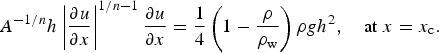(4c)$$A^{ - 1/n}h\left \vert {\displaystyle{{\partial u} \over {\partial x}}} \right \vert ^{1/n - 1}\displaystyle{{\partial u} \over {\partial x}} = \displaystyle{1 \over 4}\left( {1 - \displaystyle{\rho \over {\rho _{\rm w}}}} \right)\rho gh^2,\quad {\rm at}\;x = x_{\rm c}.$$

Additionally, we require the ice thickness, velocity and extensional stress to be continuous across the grounding line at x _g. Note that this model is only well-posed if the calving front position is directly or indirectly specified, for example through an extra condition on the ice-shelf length or ice thickness at the calving front. Since we are interested in steady-state ice shelves, the calving front position is constant in either scenario.

In the analysis described below, we first consider the dynamics of the ice shelf separately from the grounded ice sheet. We then use these results together with the continuity conditions on stress and ice thickness at the ice-stream/ice-shelf junction – the grounding line – to determine the steady-state behaviour of a confined ice-stream/ice-shelf system. This approach allows us to explicitly determine the backstress and ice flux at the grounding line, and to investigate grounding line stability for different geometric configurations and lateral-shear conditions.

3.1 Non-dimensionalisation of the ice shelf

By non-dimensionalising (1a)–(4c), we aim to simplify these equations as much as possible and reduce the number of free parameters to a minimum. We choose as characteristic length scale [x]_s the ice-shelf length L _s = x _c − x _g and set x = [x]_sx* + x _g. This leads to non-dimensional ice-shelf domain reaching from x* = 0 (the grounding line) to x* = 1 (the calving front). Moreover, we consider the ice thickness h _g and the ice flux q _g at the grounding line as given scales and identify [h]_s = h _g and [u]_s[h]_s = q _g with u _g = q _g/h _g the velocity at the grounding line. We set x = [x]_sx* + x _g, u = [u]_su*, h = [h]_sh*, as well as 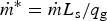$\dot m^* = \dot mL_{\rm s}/q_{\rm g}$. This leads to two non-dimensional parameters

(6)$$\eta = \displaystyle{{4A^{ - 1/n}h_{\rm g}u_{\rm g}^{1/n} L_{\rm s}^{ - 1/n}} \over {\rho g(1 - \rho /\rho _{\rm w})h_{\rm g}^2}}, \quad \beta = 2\displaystyle{{\Lambda h_{\rm g}u_{\rm g}^p L_{\rm s}} \over {\rho g(1 - \rho /\rho _{\rm w})h_{\rm g}^2}} $$

which describe the entire dynamics of the system. The parameter η is the ratio between the scale of the extensional stress at the grounding line and the scale of the driving stress at the grounding line and β is the ratio between the scale of the lateral shear stress at the grounding line and the scale of the driving stress at the grounding line. Characteristic values of these parameters for Petermann glacier (North-West Greenland), with L _s = 65 km, W = 15 km, h _g = 500 m, u _g = 1000 m/year, and the parameters listed in table 1, are η ≈ 0.8 and β ≈ 3.6. For Pine Island (West Antarctica), with L _s = 55 km, W = 40 km, h _g = 750 m and u _g = 1500 m/year, they are η ≈ β ≈ 0.6. It is important to note that this non-dimensionalisation does not change the dynamics of the ice-shelf system (see, e.g. Holmes, Reference Holmes2009; Fowler, Reference Fowler2011), it merely reformulates the mathematical problem in a way that is convenient for a solution with matched asymptotic expansions.

Table 1.

List of parameters with their value, where applicable

The non-dimensional versions of the ice-shelf stress balance (1b) and the mass balance (3) are (with the asterisks discarded)

(7a)$$\displaystyle{\partial \over {\partial x}}\left( {\eta h{\left \vert {\displaystyle{{\partial u} \over {\partial x}}} \right \vert} ^{1/n - 1}\displaystyle{{\partial u} \over {\partial x}}} \right) - \beta h \vert u \vert ^{\,p - 1}u - 2h\displaystyle{{\partial h} \over {\partial x}} = 0,$$

(7b)$$\displaystyle{{\partial (uh)} \over {\partial x}} = \dot m.$$

The boundary conditions (4b) and (4c) are

(8a)$$h = 1\quad {\rm and}\quad u = 1\quad {\rm at}\;x = 0,$$

(8b)$$\eta h\left \vert {\displaystyle{{\partial u} \over {\partial x}}} \right \vert ^{1/n - 1}\displaystyle{{\partial u} \over {\partial x}} = h^2\quad {\rm at}\;x = 1.$$

With these boundary conditions, (7b) can be easily integrated:

(9)$$uh = 1 + \dot mx.$$

One advantage of the scaling introduced here is a considerable simplification of the boundary conditions and dimensions of the domain. All information about the ice-shelf length, thickness and flux at the grounding line is now contained in the non-dimensional parameters β and η. The ratio β/η equals the ratio between the scales of the lateral shear stress and the extensional stress (6), so η ≪ β corresponds to the parameter regime where we expect lateral shear stresses to balance most of the driving stress. Therefore, we refer to this parameter regime (η ≪ β) as the limit of strong buttressing.

3.2. Exact solution

To illustrate the general idea underlying the derivations in this paper, we start by considering the linear parameterisation of the lateral shear term with p = 1 and (2)₃. In this case, it is possible to obtain an expression for the stress at the grounding line by integrating (7a) with (9) (Pegler, Reference Pegler2016)

(10)$$\tau _0 = 1 - \beta \int\limits_0^1 {hu{\rm d}x = 1 - \beta} \left( {1 + \displaystyle{{\dot m} \over 2}} \right)\quad {\rm for}\;p = 1.$$

This expression is valid for 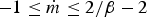$ - 1 \le \dot m \le 2/\beta - 2$. The lower bound arises from the requirement that the ice flux is non-negative. The upper bound on $\dot m$ (or alternatively β) is a requirement that the backstress at the grounding line has to be non-negative as well.

In dimensional form, the stress (10) can be written as

(11)$$\tau _{\rm g} = \tau _{{\rm g},0} \times \Theta, $$

with

(12)$$\tau _{{\rm g},0} = \displaystyle{1 \over 2}\rho g\left( {1 - \displaystyle{\rho \over {\rho _{\rm w}}}} \right)h_{\rm g}^2 $$

the grounding line stress of unbuttressed marine ice sheets and

(13)$$\Theta = \tau _0 = 1 - \displaystyle{{2\Lambda L_{\rm s}(q_{\rm g} + 1/2\dot mL_{\rm s})} \over {\rho g(1 - \rho /\rho _{\rm w})h_{\rm g}^2}}. $$

Schoof (Reference Schoof:2007b) states that if buttressing changes the unbuttressed stress at the grounding line by a factor of Θ < 1, i.e. τ _g = τ _g,0 × Θ, then this changes the flux at the grounding line by a factor of Θ^n/(m+1), i.e.

(14)$$q_{\rm g} = q_{{\rm g},0} \times \Theta ^{n/(m + 1)}$$

where

(15)$$q_{{\rm g},0} = \left( {\displaystyle{{A{(\rho g)}^{n + 1}(1 - \rho /\rho _w)} \over {4^nC}}} \right)^{1/(m + 1)}h_{\rm g}^{(3 + m + n)/(m + 1)} $$

is the ice flux of unconfined and hence unbuttressed marine ice sheets (Schoof, Reference Schoof2007a). For the linear case considered here, this means that the ice flux at the grounding line can be written as

(16)$$\eqalign{q_{\rm g} = & \left( {\displaystyle{{A{(\rho g)}^{n + 1}(1 - \rho /\rho _w)} \over {4^nC}}} \right)^{1/(m + 1)}h_{\rm g}^{(3 + m + n)/(m + 1)} \cr & \times \left( {1 - \displaystyle{{2\Lambda L_{\rm s}(q_{\rm g} + 1/2\dot mL_{\rm s})} \over {\rho g(1 - \rho /\rho _{\rm w})h_{\rm g}^2}}} \right)^{n/(m + 1)}.} $$

There are several important things we can learn from this simple solution. First, Θ ≤ 1, so buttressing always reduces the ice flux through the grounding line. Secondly, the amount by which the ice flux is reduced depends itself on the ice flux through the grounding line, and finally, the ice flux also depends on the ice-shelf geometry through the ice-shelf length L _s and width W (hidden in Λ (2)). We discuss these properties in detail in Section 5.

For p = 1/n < 1, it is not straightforward to integrate h|u|^1/n−1u. To derive Θ, we therefore construct an approximate solution using matched asymptotic expansions (Hinch, Reference Hinch1991; Holmes, Reference Holmes2013) based on the assumption that η ≪ β. This corresponds to the limit of strong buttressing where the extensional stresses are small compared to the lateral shear stresses in the ice shelf (see (6)).

3.3. Asymptotic solutions

In this section, we construct solutions for the velocity field in strongly buttressed ice shelves by using matched asymptotic expansions (see for example chapter 5 of Hinch (Reference Hinch1991) or chapter 2 of Holmes (Reference Holmes2013)). In this approach, we assume the perturbation parameter η to be small (for a discussion of this assumption see Section 3.4). If η ≪ 1, then the solutions u and h can be expanded in terms of η, e.g. u = u ⁽⁰⁾ + ηu ⁽¹⁾ + O(η ²). This allows us to neglect terms of O(η) in the main part of the ice shelf, termed the ‘outer’ region, and we can derive a simplified ‘outer’ solution in this part of the ice shelf. However, this outer solution cannot satisfy the boundary conditions at the grounding line, where the extensional stress becomes non-negligible. To satisfy these boundary conditions, we introduce a boundary layer at the grounding line in which we rescale the ice-shelf equations. Solution of these rescaled boundary layer equations leads to the so-called ‘inner’ solution. Finally, by matching the inner and outer solution, we can then construct an approximate solution (called a ‘composite solution’ in the literature on matched asymptotic expansions) valid in the entire shelf. We can use this composite solution to determine the stress at the grounding line τ _g. The remainder of this section describes the construction of the composite velocity solution for ice shelves that exhibit a boundary layer structure. Readers not interested in technical details of the derivation can proceed to Section 3.4 where the main results are summarised.

We start by deriving the outer solution (h ⁽⁰⁾ and u ⁽⁰⁾), obtained by neglecting terms of O(η) in the momentum balance (7a) and assuming that η ≪ β ~ 1:

(17a)$$- \beta h^{(0)} \vert u^{(0)} \vert ^{\,p - 1}u^{(0)} - 2h^{(0)}\displaystyle{{\partial h^{(0)}} \over {\partial x}} = 0$$

with the boundary conditions

(17b)$$h^{(0)} = 1\quad {\rm and}\quad u^{(0)} = 1\quad {\rm at}\;x = 0,$$

(17c)$$h^{(0)} = 0\quad {\rm at}\;x = 1.$$

Keeping in mind that 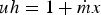$uh = 1 + \dot mx$, (17a) is really just a first-order equation in either u ⁽⁰⁾ or h ⁽⁰⁾, and we proceed by solving for the velocity u ⁽⁰⁾. Note that we have two boundary conditions for u ⁽⁰⁾ (h ⁽⁰⁾ = 0 is the same as requiring u ⁽⁰⁾ → ∞), but (17a) is only a first-order differential equation. Therefore, we can only expect to satisfy one of the boundary conditions.

The velocity and flux should be non-negative ($u^{(0)} \ge 0,1 + \dot mx \ge 0)$, so that (17a) can be integrated to obtain (Pegler, Reference Pegler2016)

(18)$$u^{(0)}(x) = \displaystyle{{1 + \dot mx} \over {{\left( {h_{1,{\rm butt}}^{\,p + 1} + \beta /(2\dot m)\left[ {{(1 + \dot m)}^{\,p + 1} - {(1 + \dot mx)}^{\,p + 1}} \right]} \right)}^{1/(p + 1)}}},$$

which satisfies the calving front boundary condition (17c) if h _1,butt = 0. This leads to an infinite leading order velocity at the calving front at x = 1. However, this excludes the possibility of later investigating the effect of ice-thickness-based calving laws (e.g. Nick and others, Reference Nick, Vieli, Howat and Joughin2009). One way to include a non-zero ice thickness at the calving front is to follow Pegler (Reference Pegler2016), who determines h _1,butt by applying the boundary condition (8b) instead of (17c). This leads to (Pegler, Reference Pegler2016)

(19)$$h_{1,{\rm butt}} = \left[ {\eta ^n\displaystyle{\beta \over 2}{(1 + \dot m)}^{\,p + 1}} \right]^{1/(2 + n + p)}.$$

As discussed in Pegler (Reference Pegler2016), this matches the ice thickness at the calving front obtained by numerical solution of (7a) and (8b) to an error of < 2%, and leads to a better match between numerically calculated velocity fields in the main part of the ice shelf and (18). We show in the Supplementary material (Section S1) that this approach is consistent with the introduction of a boundary layer at the calving front.

The outer solution (18) does not satisfy the boundary conditions (8a) at x = 0, which requires us to introduce a boundary layer by rescaling of the downstream coordinate with x = η ⁿX (e.g. Holmes, Reference Holmes2013). To distinguish the ice thickness and velocity in the boundary layer from the outer variables we denote these with H and U, respectively. With these definitions, we obtain from (7) and (8) the boundary layer equations (neglecting terms of O(η ⁿ) as we again assume that a series expansion of u and h in terms of η is possible):

(20a)$$\displaystyle{\partial \over {\partial X}}\left( {H{\left \vert {\displaystyle{{\partial U} \over {\partial X}}} \right \vert} ^{1/n - 1}\displaystyle{{\partial U} \over {\partial X}}} \right) - 2H\displaystyle{{\partial H} \over {\partial X}} = 0,$$

(20b)$$UH = 1$$

with the boundary conditions

(20c)$$U = H = 1\quad {\rm at}\quad X = 0,$$

and the matching conditions

(20d)$$\left. {\matrix{ {U{\rm \sim} u^{(0)}} \hfill \cr {H{\rm \sim} h^{(0)}} \hfill \cr}} \right\}\quad {\rm as}\;X \to \infty, {\kern 1pt} x \to 0.$$

We can integrate (20a) to obtain

(21)$$\tau _0 - H\left \vert {\displaystyle{{\partial U} \over {\partial X}}} \right \vert ^{1/n - 1}\displaystyle{{\partial U} \over {\partial X}} = 1 - H^2,$$

where τ ₀ is the non-dimensional version of the extensional stress at the grounding line τ _g:

(22)$$\tau _0 = H\left \vert {\displaystyle{{\partial U} \over {\partial X}}} \right \vert ^{1/n - 1}\displaystyle{{\partial U} \over {\partial X}} = \eta h\left \vert {\displaystyle{{\partial u} \over {\partial x}}} \right \vert ^{1/n - 1}\displaystyle{{\partial u} \over {\partial x}}\quad {\rm at}\;X = x = 0,$$

which we aim to determine here. Using H = 1/U (20b), we can rewrite (21) as

(23)$$\left \vert {\displaystyle{{\partial U} \over {\partial X}}} \right \vert ^{1/n - 1}\displaystyle{{\partial U} \over {\partial X}} = \displaystyle{1 \over U} - U(1 - \tau _0).$$

This leads to the integral equation

(24)$$\int\limits_0^X {{\rm d}{X}^{\prime} = \int\limits_1^U {\displaystyle{{V^n{\rm d}V} \over {{[1 - (1 - \tau _0)V^2]}^n}},}} $$

which determines the boundary layer velocity U implicitly.

For n > 0, the solution of (24) can be written as

(25)$$X = \displaystyle{1 \over {(n + 1)}}\left[ {U^{1 + n}{\kern 1pt} _2F_1\left( {n,\displaystyle{{n + 1} \over 2};\displaystyle{{n + 3} \over 2};(1 - \tau _0)U^2} \right)} \right]_1^U, $$

where ₂ F ₁(a, b;c;x) is the hypergeometric function, and the subscript and superscript denote the lower and upper integration limits. There is no closed form expression for the inverse of the hypergeometric function for an arbitrary value of n, which would allow us to explicitly give U = f ⁻¹(X). However, for the typically assumed value of n = 3, we can write U = f ⁻¹(X) as (Abramowitz and Stegun, Reference Abramowitz and Stegun1964)

(26)$$U = \displaystyle{1 \over {\sqrt {1 - \tau _0}}} \left[ {\left( {\displaystyle{{1 + Y} \over Y}} \right)\left( {1 + \sqrt {\displaystyle{1 \over {1 + Y}}}} \right)} \right]^{1/2}$$

with $Y = 4(1 - \tau _0)^2X + (1 - 2\tau _0)/\tau _0^2 $.

The extensional stress at the grounding line (τ ₀) must be determined by matching the solutions for the boundary layer velocity U and the outer solution u ⁽⁰⁾ (18), i.e. from the condition U ~ u ⁽⁰⁾ for X → ∞, x → 0, (20d)₁ (Holmes, Reference Holmes2013). For n = 3, we can use (26) to determine U ~ (1 − τ ₀)^−1/2 for X → ∞. For an arbitrary n, we can exploit the fact that the right-hand side of (24) has a pole at U = (1 − τ ₀)^−1/2, which determines the limiting behaviour for X → ∞ (a vertical pole in the inverse function turns into a horizontal pole in the forward function). Thus,

$$U \to (1 - \tau _0)^{ - 1/2}\quad {\rm as}\;X \to \infty, $$

which has to match the asymptotic behaviour of the outer solution u ⁽⁰⁾ (18) as x → 0:

$$u^{(0)} \to \left( {h_{1,{\rm butt}}^{\,p + 1} + \displaystyle{\beta \over {2\dot m}}[(1 + \dot m)^{\,p + 1} - 1]} \right)^{ - 1/(\,p + 1)}\quad {\rm as}\;x \to 0.$$

Hence, the matching condition (20d)₁ becomes

(27)$$\eqalign{(1 -& \tau _0)^{ - 1/2}{\rm \sim} \left( {h_{1,{\rm butt}}^{\,p + 1} + \displaystyle{\beta \over {2\dot m}}[(1 + \dot m)^{\,p + 1} - 1]} \right)^{ - 1/(\,p + 1)} \cr & {\rm as}\;X \to \infty, x \to 0,}$$

which provides us with an expression for the stress at the grounding line τ ₀

(28)$$\tau _0 = 1 - \left( {h_{1,{\rm butt}}^{\,p + 1} + \displaystyle{\beta \over {2\dot m}}[(1 + \dot m)^{\,p + 1} - 1]} \right)^{2/(\,p + 1)}$$

with h _1,butt given by (19). At this point, we have all the information we need to determine the ice flux at the grounding line.

Finally, it is possible to obtain the composite velocity field through the superposition of the inner solution U (25) and the outer solution u ⁽⁰⁾ (18) minus the overlap term (1 − τ ₀)^−1/2 shared by both solutions (e.g. Holmes, Reference Holmes2013):

(29)$$u = u^{(0)} + U - (1 - \tau _0)^{ - 1/2}.$$

For n = 3, this yields

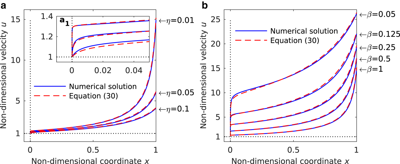
(30)$$\eqalign{u = & \displaystyle{{(1 + \dot mx)} \over {{\left( {h_{1,{\rm butt}}^{\,p + 1} + \beta /(2\dot m)\left[ {{(1 + \dot m)}^{\,p + 1} - {(1 + \dot mx)}^{\,p + 1}} \right]} \right)}^{1/(p + 1)}}} \cr & + \left[ {\displaystyle{1 \over {1 - \tau _0}}\left( {\displaystyle{{1 + Y} \over Y}} \right)\left( {1 + \sqrt {\displaystyle{1 \over {1 + Y}}}} \right)} \right]^{1/2} \cr & - \displaystyle{1 \over {{(1 - \tau _0)}^{1/2}}}} $$

with $Y = 4\eta ^{ - 3}(1 - \tau _0)^2x + (1 - 2\tau _0)/\tau _0^2. $ In Fig. 2, we compare the composite solution (30) with numerical solutions obtained by solving the unsimplified non-dimensional ice-shelf equations (7a) and (8b) for either different values of η and β fixed, or η fixed and β varying. In both cases, the match between the composite and numerical solutions improves as the ratio β/η increases. This is not surprising since β/η ≫ 1 is the limit for which the solutions derived here are valid. As η is reduced, the boundary layer at the grounding line becomes more pronounced (see inset a ₁). Conversely, increasing β leads to steeper velocity gradients towards the calving front (see panel (b)).

Fig. 2.

Velocity profiles in the ice shelf. Panel (a) shows a comparison of numerical solutions and composite solutions u (30) in the ice shelf for different η as indicated, and $n = 1/p = 3,\dot m = 0,\beta = 1$. The grounding line is located at x = 0, the calving front is located at x = 1. Note that the boundary layer at the grounding line becomes more pronounced as η decreases and that the match between numerical and composite solution improves as η decreases (see inset panel a ₁). Panel (b) shows a comparison of numerical solutions and composite solutions in the ice shelf for different β as indicated, and $n = 1/p = 3,\dot m = 0,\eta = 10^{ - 2}$. Numerical solutions are obtained by direct solution of the unsimplified equations (7a) and (8b) with Matlab ODE solvers and a shooting method.

3.4 Analysis of the ice-shelf solution

In the last section, we have exploited the boundary layer structure of strongly buttressed ice shelves to derive solutions for the velocity (30) and the stress at the grounding line (28) for a non-linear lateral shear stress term (p < 1 in (2)). The flow in the main part of the ice shelf can be described by a leading order balance between the lateral shear stress and driving stress (Hindmarsh, Reference Hindmarsh2012), and its solution (18) has previously been derived in Pegler (Reference Pegler2016). The main difference between our ice-shelf solution and the solutions considered in Pegler (Reference Pegler2016) and Hindmarsh (Reference Hindmarsh2012) is that we explicitly introduce a boundary layer at the grounding line which ensures that the boundary conditions at the grounding line are satisfied. The existence of this boundary layer is noted in Pegler (Reference Pegler2016), who also discusses its properties. Solution of the leading order equations in this boundary layer allows us to determine the backstress at the grounding line τ ₀ by using matched asymptotic expansions (Hinch, Reference Hinch1991; Holmes, Reference Holmes2013), which provides us with an avenue to determine the ice flux at the grounding line through (14).

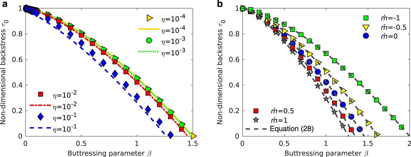
The boundary layer treatment of the ice-shelf equations at the grounding line and the derivation of the backstress τ ₀ relies on the assumption that η is small and that terms of O(η) can be neglected in the main part of the ice shelf. The size of η is determined by the ice-shelf properties (see (6)) and it is not guaranteed that η ≪ 1. We therefore validate our equation for the grounding line stress (28) by comparing it with numerical solutions of the unsimplified non-dimensional ice-shelf equations (7a) to (8b) obtained with Matlab ODE solvers together with a shooting method to determine the correct grounding line stress τ ₀. Figure 3 shows numerical and asymptotic solutions of the grounding line stress τ ₀ (28) for different values of the non-dimensional viscosity η (panel a) and accumulation rate $\dot m$ (panel (b)). There is good agreement between the asymptotic and the numerical solutions for η ≤ 10⁻². Note that there is a viscosity-dependence of τ ₀ which decreases for η → 0, i.e. τ ₀ converges to a viscosity-independent value as η → 0, the limit where lateral shear stresses balance most of the driving stress. Note also that the asymptotic solutions appear to remain valid all the way up to β = 0.

Fig. 3.

Comparison of asymptotic solutions and numerical solutions of the stress at the grounding line. Markers are numerical solutions obtained by solving the unsimplified non-dimensional problem (7a) to (8b) with Matlab ODE solvers and a shooting method, lines are the asymptotic solution (28). (a) Non-dimensional backstress τ ₀ vs the buttressing parameter β for $\dot m = 0$ and different values of η, as indicated in the legend. Note that $[(1 + \dot m)^{p + 1} - 1]/\dot m = p + 1$ at $\dot m = 0$. (b) Non-dimensional backstress τ ₀ vs the buttressing parameter β, for different accumulation rates and η = 10⁻². p = 1/n = 1/3 for all calculations.

The asymptotic solution captures this viscosity dependence via the expression for the ice thickness at the calving front h _1,butt (19). This is qualitatively different from the linearised case for p = 1, where the exact formula (10) predicts that the stress τ ₀ is independent of the viscosity and the ice thickness at the calving front. However, this also implies that the boundary layer solution (28) agrees with the exact solution for p = 1 (10) in the limit of η → 0 (where h _1,butt → 0) only.

We have explicitly included the term h _1,butt (19) in our expression of the grounding line stress (28) in order to later test calving laws that are based on the ice thickness at the calving front. However, we expect h _1,butt (19) to provide a valid approximation for the ice thickness at the calving front for η ≪ β ~ 1 only, as this is the limit in which the outer solution was derived. This is confirmed by a comparison of (19) with numerical solutions of (7) and (8) for constant η but different values of β and either $\dot m = 0$ or $\dot m = 1$ in Fig. 4 (for $\dot m = - 1$ the ice thickness at the calving front is zero: h _c = h _c,butt = 0). Figure 4 illustrates that h _1,butt and the numerical solution of the ice thickness at the calving front only agree for $\beta /\eta \mathop \gt \limits_ \approx 1.$. For $\beta /\eta \mathop \lt \limits_ \approx 1, {h_{1,{\rm butt}}}$ decreases with decreasing β, while the numerical solution converges towards the value for the calving front ice thickness of unbuttressed ice shelves (Van der Veen, Reference Van der Veen1983, referenced as (32) below).

Fig. 4.

Comparison of the different solutions for the non-dimensional ice thickness at the calving front, plotted against the buttressing strength β/η for non-dimensional accumulation $\dot m = 0$ and $\dot m = 1$. h _1,butt is the asymptotic solution for buttressed ice shelves (19), h _1,unbutt is the exact solution for unconfined ice shelves (32), h ₁ is the approximate solution (31), and numerical results are obtained by solving the unsimplified non-dimensional ice shelf Eqns (7a) to (8b). η = 10⁻², n = 1/p = 3.

This deviation does not affect the prediction of the backstress at the grounding line and the flux at the grounding line unless the ice thickness at the grounding line is explicitly set by a calving law. In this case, we approximate the ice thickness at the calving front with

(31)$$h_1^{2 + n + p} = h_{1,{\rm butt}}^{2 + n + p} {\rm erf}\left( {\displaystyle{\beta \over \eta}} \right) + h_{1,{\rm unbutt}}^{2 + n + p} {\rm erfc}\left( {\displaystyle{\beta \over \eta}} \right),$$

where h _1,butt is given by (19) and h _1,unbutt is given by (Van der Veen, Reference Van der Veen1983)

(32)$$h_{1,{\rm unbutt}} = \displaystyle{{(1 + \dot m)} \over {{(1 + 1/(\eta ^n\dot m)[{(1 + \dot m)}^{n + 1} - 1])}^{1/(n + 1)}}}.$$

Note that (31) is an approximation which is chosen purely heuristically because of its simplicity and because it correctly reproduces the asymptotic behaviour for β/η ≫ 1 and β/η ≪ 1. Therefore, we cannot expect to correctly match the transition between these two asymptotic limits, which is apparent for the solutions plotted in Fig. 4. However, as we will see in Section 5, h ₁ is a useful tool for interpreting grounding line positions. In the Supplementary material, we compare (31) with an exact solution for the special case of n = p = 1 and $\dot m = 0$, which is derived in Pegler (Reference Pegler2016).

Requiring the stress at the grounding line (28) to be positive constraints β:

(33)$$\eta {\rm \ll} \beta \le \left( {1 - h_1^{\,p + 1}} \right)\displaystyle{{2\dot m} \over {{(1 + \dot m)}^{\,p + 1} - 1}}.$$

Two other conditions – a positive ice-shelf length, and a positive ice thickness at the calving front, which should also be less than the ice thickness at the grounding line (0 ≤ h ₁ < 1) – provide constraints on the maximum net mass loss over the ice shelf $ - \dot mL_{\rm s}$. This mass loss must be equal or less than the ice flux at the grounding line:

$$- \dot mL_{\rm s} \le q_{\rm g}\quad {\rm if}\;\dot m \lt 0\quad {\rm and}\quad L_{\rm s} \gt 0.$$

The dimensional forms of the derived expressions are the following: the extensional stress τ _g is

(34a)$$\tau _{\rm g} = \tau _{{\rm g},0} \times \Theta _{{\rm general}}$$

with τ _g,0 given by (12) and

(34b)$$\Theta _{{\rm general}} = \left( {1 - {\left[ {\displaystyle{{h_{{\rm c},{\rm butt}}^{\,p + 1}} \over {h_{\rm g}^{\,p + 1}}} + \Lambda \displaystyle{{{(q_{\rm g} + \dot mL_{\rm s})}^{\,p + 1} - q_{\rm g}^{\,p + 1}} \over {\rho g(1 - \rho /\rho _{\rm w})\dot mh_{\rm g}^{\,p + 1}}}} \right]}^{2/(p + 1)}} \right)$$

(note that for $\dot m = 0$ we have $[(q_{\rm g} + \dot mL_{\rm s})^{p + 1} - q_{\rm g}^{p + 1} ]/ \dot m = (p + 1)q_{\rm g}^p L_{\rm s} $). In contrast to the unbuttressed case, where the grounding line stress τ _g,0 (12) depends only on the ice thickness at the grounding line h _g and local ice and bed properties, the buttressed stress also depends on the length of the ice shelf L _s, the ice flux at the grounding line q _g, the accumulation/melt rate on the shelf $\dot m$ and the width of the ice shelf W through Λ (Eqn (2)). Additionally, the grounding line stress depends on h _c,butt, given by (19)

(35)$$h_{{\rm c},{\rm butt}} = \left[ {\Lambda \displaystyle{{{(4A^{ - 1/n})}^n} \over {{((1 - \rho /\rho _{\rm w})\rho g)}^{n + 1}}}{(q_{\rm g} + \dot mL_{\rm s})}^{\,p + 1}} \right]^{1/(2 + n + p)}.$$

In the limit of strong buttressing, h _c,butt corresponds to the ice thickness at the calving front h _c (Pegler, Reference Pegler2016), which we approximate by (31)

(36)$$\eqalign{h_{\rm c} = & \left[ {h_{{\rm c},{\rm butt}}^{2 + n + p} {\rm erf}\left( {\displaystyle{1 \over 2}\Lambda u_{\rm g}^{\,p - 1/n} L_{\rm s}^{1 + 1/n} A^{1/n}} \right)} \right. \cr & + \left. {h_{{\rm c},{\rm unbutt}}^{2 + n + p} {\rm erfc}\left( {\displaystyle{1 \over 2}\Lambda u_{\rm g}^{\,p - 1/n} L_{\rm s}^{1 + 1/n} A^{1/n}} \right)} \right]^{1/(2 + n + p)},} $$

with h _c,unbutt the calving front ice thickness of an unconfined ice shelf from (32):

(37)$$\eqalign{h_{{\rm c},{\rm unbutt}} = & \left( {q_{\rm g} + \dot mL_{\rm s}} \right) \times \bigg[\left( {\displaystyle{{q_{\rm g}} \over {h_{\rm g}}}} \right)^{n + 1} + A\left( {\displaystyle{{\rho g} \over 4}\left( {1 - \displaystyle{\rho \over {\rho _{\rm w}}}} \right)} \right)^n \cr & \times \left. {\displaystyle{1 \over {\dot m}}\left( {{(q_{\rm g} + \dot mL_{\rm s})}^{n + 1} - q_{\rm g}^{n + 1}} \right)} \right]^{ - 1/(n + 1)}.} $$

Note that the ice thickness at the calving front h _c,butt (35) directly depends on the flux at the grounding line. If the net accumulation over the shelf is zero $(\dot m = 0)$ the calving front ice thickness and the flux at the grounding line appear to be explicitly linked: $h_{{\rm c},{\rm butt}}{\rm \sim} q_{\rm g}^{(1 + p)/(2 + n + p)} $. We will discuss the implications of this in Section 5.

As outlined in Section 3.2, we can now use (34b) to determine the ice flux at the grounding line from (14), i.e.

(38)$$q_{\rm g} = q_{q,0} \times \Theta _{{\rm general}}^{n/(m + 1)} $$

without having to solve the grounding line problem considered in (Schoof, Reference Schoof2007a). This accomplishes the goal of this section, even though the resulting expression for q _g is relatively complicated (we explicitly write it out in (44)).

5.1 Simplified marine ice-sheet model

Using the results of the previous sections, a simplified model for steady-state marine ice sheets can be considered in lieu of the full problem (1)–(4c). The momentum balance (1a) and mass balance (3) of the grounded ice sheet are simplified per (42a) (see also Schoof, Reference Schoof2007a)

(43a)$$\hskip-4pt \left. {\matrix{ { - C \vert u \vert ^{m - 1}u - \Lambda h \vert u \vert ^{\,p - 1}u - \rho gh\displaystyle{{\partial (h + b)} \over {\partial x}} = 0} \hfill \cr {\displaystyle{{\partial (uh)} \over {\partial x}} = \dot a} \hfill \cr {h \ge - \displaystyle{{\rho _{\rm w}} \over \rho} b} \hfill \cr}}\!\! \right\}x \in (0,x_{\rm g})$$

with the boundary conditions at ice divide and grounding line from (42b)and (42c):

(43b)$$\displaystyle{{\partial (h + b)} \over {\partial x}} = q = 0\quad {\rm at}\;x = 0,$$

(43c)$$h = h_{\rm g} = - \displaystyle{{\rho _{\rm w}} \over \rho} b\quad {\rm and}\quad q = q_{\rm g}\quad {\rm at}\;x = x_g.$$

The effect of an ice shelf is captured by the implicit expression for the ice flux at the grounding line q _g (38) with (34b):

(44)$$\eqalign{q_{\rm g} = & \left( {\displaystyle{{A{(\rho g)}^{n + 1}{\left( {1 - \rho /\rho _{\rm w}} \right)}^n} \over {4^nC}}} \right)^{1/(m + 1)}h_{\rm g}^{(3 + m + n)/(m + 1)} \cr & \times \left( {1 - {\left[ {\displaystyle{{h_{{\rm c},{\rm butt}}^{\,p + 1}} \over {h_{\rm g}^{\,p + 1}}} + \Lambda \displaystyle{{{(q_{\rm g} + \dot mL_{\rm s})}^{\,p + 1} - q_{\rm g}^{\,p + 1}} \over {\rho g\left( {1 - \rho /\rho _{\rm w}} \right)\dot mh_{\rm g}^{\,p + 1}}}} \right]}^{2/(p + 1)}} \right)^{n/(m + 1)}} $$

q _g now depends not only on the ice thickness at the grounding line, but also on the length of the ice shelf L _s, the width W of the ice shelf through Λ in (2), and h _c,butt (35).

For strongly buttressed ice shelves, we can replace (44) with the dimensional version of (42c):

(45)$$\displaystyle{{{(q_{\rm g} + \dot mL_{\rm s})}^{\,p + 1} - q_{\rm g}^{\,p + 1}} \over {\dot m}} = \displaystyle{{\rho g(1 - \rho /\rho _{\rm w})} \over \Lambda} h_{\rm g}^{\,p + 1}. $$

There are two noteworthy special cases of (45): if there is zero net accumulation, we get

(46a)$$q_{\rm g} = \left( {\displaystyle{{\rho g(1 - \rho /\rho _{\rm w})} \over {(\,p + 1)\Lambda L_{\rm s}}}} \right)^{1/p}h_{\rm g}^{1 + 1/p}, \quad {\rm if}\;\dot m = 0$$

as $[(q_{\rm g} + \dot mL_{\rm s})^{p + 1} - q_{\rm g}^{p + 1} ]/\dot m = (p + 1)q_{\rm g}^p L_s$ at $\dot m = 0$. Alternatively, if all the mass of the ice shelf is lost through melting, that is in the absence of calving, we have $L_{\rm s} = q_{\rm g}/( - \dot m)$ and obtain

(46b)$$q_{\rm g} = \left[ {\rho g\left( {1 - \displaystyle{\rho \over {\rho _{\rm w}}}} \right)\displaystyle{{ - \dot m} \over \Lambda}} \right]^{1/(p + 1)}h_{\rm g},\quad {\rm if}\left\{ {\matrix{ {\dot m \lt 0,} \hfill \cr {L_{\rm s} = \displaystyle{{q_{\rm g}} \over {( - \dot m)}}.} \hfill \cr}} \right.$$

We write (46a) and (46b) out here as these explicit expressions for the ice flux are easier to understand than their more complicated implicit counterparts. In particular, we can see from (46a) and (46b) that in the limit of strong buttressing, the ice flux at the grounding line is again a function of the ice thickness at the grounding line, and that the exponent on the ice thickness strongly depends on the mechanism through which the ice shelf loses its mass (i.e. q _g ∝ h ^1+1/p for calving only, q _g ∝ h _g for melting only). In contrast to the unbuttressed case (compare (15)), q _g is independent of the properties of the ice sheet, which are represented by the sliding parameters C and m in the unbuttressed flux (15). Instead, the strongly buttressed flux (46) depends only on the ice-shelf width W (which is somewhat hidden in the expression of Λ), the ice-shelf length L _s and/or net accumulation term $\dot m$. This is also true for the more general case of mixed ice-shelf calving and melting, see (45). We therefore expect the dynamics of strongly buttressed marine ice sheets to be governed by the ice-shelf properties, as also suggested from the analysis of laboratory studies in Pegler and others (Reference Pegler, Kowal, Hasenclever and Worster2013) and Kowal and others (Reference Kowal, Pegler and Worster2016).

In the next section, we use (43)–(45) to confirm these initial observations and to investigate how buttressing affects the position of the grounding line. As a test case, we choose a laterally confined version of the MISMIP experiment 1a (Pattyn and others, Reference Pattyn2012) with the ice-stream/ice-shelf system flowing in a channel of constant width W and the bed elevation given by

$$b(x) = \left( {720 - 778.5 \times \displaystyle{x \over {750\;{\rm km}}}} \right){\rm m}{\rm.} $$

In the case of a constant accumulation rate $\dot a$, we can solve (43a)₂ to obtain

(47)$$q_{\rm g} = \dot ax_{\rm g}.$$

Together with the flux expressions (44) or (45), this allows us to directly determine the grounding line position x _g. Additionally, we assume that the rate of mass gain of the ice shelf $(\dot m)$ equals the rate of mass gain of the ice sheet $(\dot m = \dot a)$. All other parameters are listed in table 1.

With the flux expressions (44) and (45), we now have three different methods to determine steady-state grounding line positions of buttressed marine ice sheets:

1. (i) semi-analytically by use of (44) in (47),

2. (ii) semi-analytically by use of (45) in (47), and

3. (iii) numerically by solution of the unsimplified system (1)–(4c).

For the numerical solution, we use the finite element solver Comsol at a resolution that is sufficiently high such that further refinement of the numerical grid does not change the numerical results. To obtain the semi-analytical solutions with (44) or (45), we have to solve the algebraic Eqn (47). While this is significantly faster than solving the system of differential Eqns (1)–(4c), a numerical algorithm is still necessary to solve these non-linear equations. We use a Newton method to determine x _g up to a relative accuracy of 10⁻⁸.

5.2 The effect of calving on the grounding line position

In the unbuttressed MISMIP experiments, it is not necessary to prescribe a calving law as the ice shelf can be excluded from the momentum balance in accordance with (15). In the buttressed case, however, computing the grounding line flux q _g from (44) or (45) requires a condition on either L _s (length of the ice shelf), x _c (position of the calving front), or h _c (ice thickness at the calving front), and prescription of the lateral drag term Λ. Here, we determine Λ from the ice-shelf width W with the formula provided by Hindmarsh (Reference Hindmarsh2012), Eqn (3)₁.

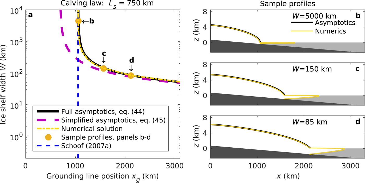
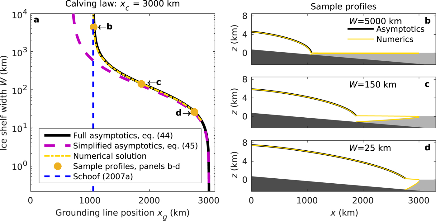
Figures 5–7 illustrate how different calving laws affect steady-state grounding line position as the ice-shelf width is reduced and buttressing increases. Figure 5 shows steady-state grounding line positions for different ice-shelf widths with a prescribed ice-shelf length L _s = 750 km. Figure 6 shows results with a prescribed calving front x _c = 3000 km, i.e. we use L _s = x _c − x _g in (44) and (45). Figure 7 shows results with a prescribed calving front thickness h _c = 250 m.

Fig. 5.

Comparison of asymptotic and numerical results for MISMIP experiment 1a (Pattyn and others, Reference Pattyn2012) with additional buttressing. Panel (a) shows ice-shelf width W vs grounding line position x _g for a fixed ice-shelf length of L _s = 750 km, and panels (b) and (d) show corresponding ice-sheet profiles. Numerical results are obtained by solving the unsimplified model (1)–(4c) numerically with Comsol. The asymptotic grounding line positions are obtained by solving $\dot ax_{\rm g} = q_{\rm g}$ (47) with q _g given by (44) and (45), respectively. The asymptotic profiles are calculated by additionally integrating (43a)–(43c). Note that the ice shelf is only plotted for the numerical solutions, as it can be excluded from the asymptotics.

Fig. 6.

Same as Fig. 5 but for a fixed calving front position at x _c = 3000 km: panel a shows ice-shelf width W vs grounding line position x _g, and panels (b) and (d) show corresponding ice-sheet profiles. Numerical results are obtained by solving the unsimplified model (1)–(4c) numerically with Comsol. The asymptotic grounding line positions are obtained by solving $\dot ax_g = q_g$ (47) with q _g given by (44) and (45), respectively. The asymptotic profiles are calculated by additionally integrating (43a)–(43c). Note that the ice shelf is only plotted for the numerical solutions, as it can be excluded from the asymptotics.

Fig. 7.

Same as Fig. 5 but with calving if ice thickness at the calving front h _c is below 250 m. Panel a shows ice-shelf width W vs grounding line position x _g, and panels (b)–(d) show corresponding ice-sheet profiles. Numerical results are obtained by solving the unsimplified model (1)–(4c) numerically with Comsol. The asymptotic grounding line positions are obtained by solving $\dot ax_{\rm g} = q_{\rm g}$ (47) with q _g given by (44) and (49), respectively. The asymptotic profiles are calculated by additionally integrating (43a)–(43c). Note that the ice shelf is only plotted for the numerical solutions, as it can be excluded from the asymptotics, and that no numerical solution exists for the profile with a grounding line at x _g ≈ 2100 km, as this solution is unstable (see Fig. 8).

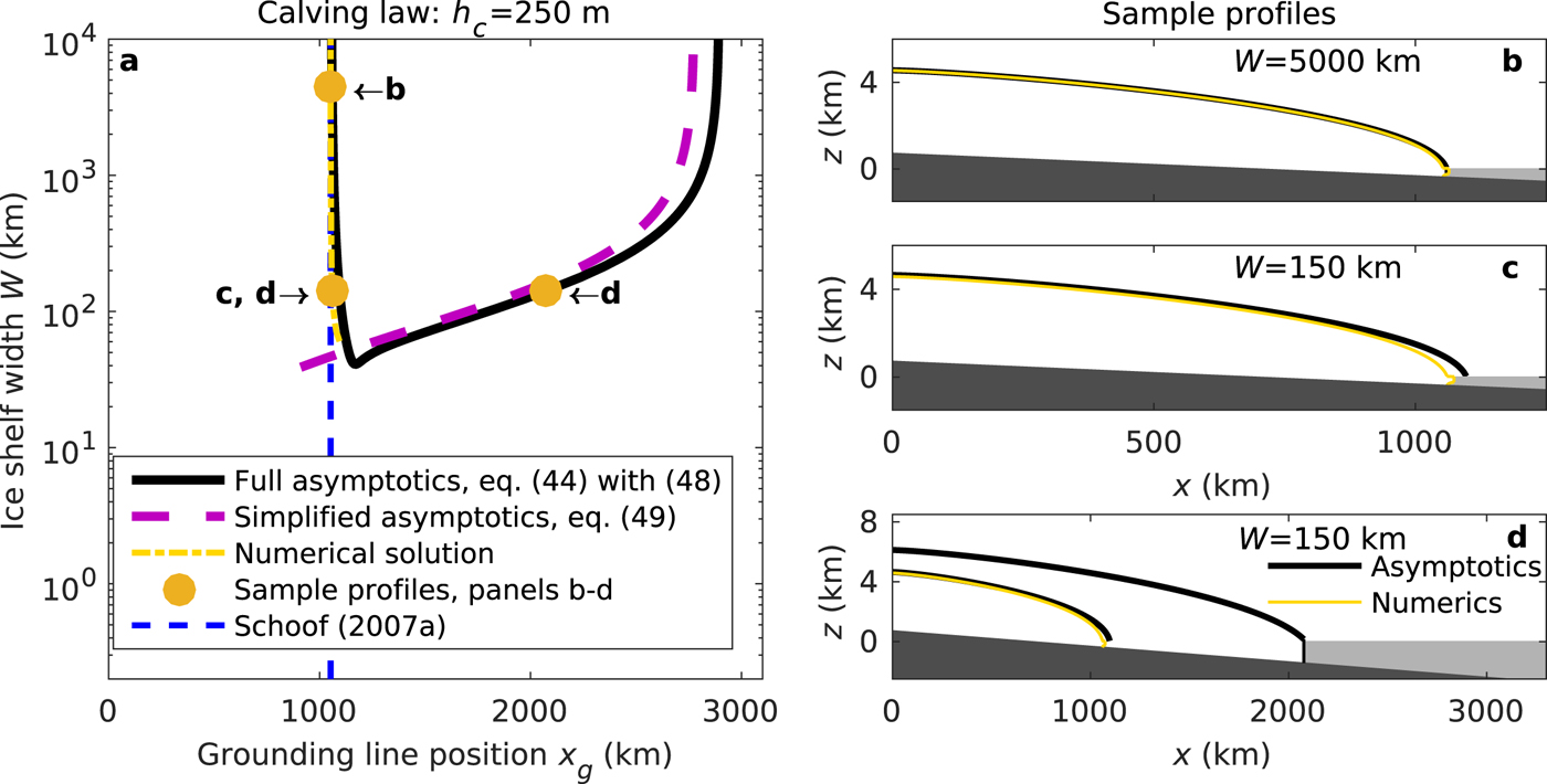
For an infinitely wide marine ice sheet (W → ∞) the solutions of the asymptotic model (44) with a fixed ice-shelf length (Fig. 5a) and with a fixed calving front position (Fig. 6a) converge to the solution for unbuttressed marine ice sheets by Schoof (Reference Schoof2007a). Decreasing the width leads to grounding line advance, which continues indefinitely for the case of a fixed ice-shelf length. Conversely, the fixed calving front position leads to the grounding line asymptotically approaching the calving front position as the ice-shelf width decreases. Comparison of the full asymptotic solutions (44) with numerical solutions of the unsimplified model (1a)–(4c) obtained with the finite-element solver Comsol shows < 2% difference of grounding line positions at any computed point (yellow dashed lines in Figs 5a, 6a, respectively).

For these two cases (x _c = const. and L _s = const., Figs 5, 6, respectively), the grounding line positions predicted by the simplified asymptotic model (45) qualitatively follow the results of the full asymptotic model, but deviate significantly towards the unbuttressed limit (for W → ∞). Results with the simplified flux converge to the full asymptotic solution and the numerical solution for $W\mathop \lt \limits_ \approx 50$, which is consistent with the limit of strong buttressing, the limit for which we derived the simplified flux expression. As (45) only depends on ice-shelf properties, these results confirm that in the limit of strong buttressing, the position of the grounding line is determined by the ice-shelf dynamics only.

Use of a calving model that prescribes calving when the ice thickness at the calving front is below a certain threshold requires us to solve (47) with (44) and (36), as we apply the boundary condition by prescribing h _c. With (2)₁, (36) can be written as

(48)$$\eqalign{h_{\rm c} = & \left[ {h_{{\rm c},{\rm unbutt}}^{2 + n + p} {\rm erfc}\left( {{(n + 1)}^{1/n}L_{\rm s}^{1 + 1/n} /W^{1 + 1/n}} \right)} \right. \cr & + \left. {h_{{\rm c},{\rm butt}}^{2 + n + p} {\rm erf}\left( {{(n + 1)}^{1/n}L_{\rm s}^{1 + 1/n} /W^{1 + 1/n}} \right)} \right]^{1/(2 + n + p)},} $$

which converges to h _c,unbutt (37) for W → ∞ and to h _c,butt (35) for W ≪ L _s.

Equation (44) with (47) and (48) implicitly provides the ice flux at the grounding line. In the limit of strong buttressing, we can again obtain an explicit equation for the grounding line flux by combining (45) with (35):

(49)$$\eqalign{q_{\rm g} = & \left( {\displaystyle{{\rho g(1 - \rho /\rho _{\rm w})} \over \Lambda}} \right)^{1/(p + 1)} \cr & \times \left[ {{\left( {\displaystyle{{\rho g} \over 4}\left( {1 - \displaystyle{\rho \over {\rho _{\rm w}}}} \right)} \right)}^nAh_{{\rm c},{\rm butt}}^{2 + n + p} - \dot mh_{\rm g}^{\,p + 1}} \right]^{1/(p + 1)}} $$

and applying the boundary condition directly to h _c,butt, i.e. h _c,butt = 250 m. As we discuss in Section 3.4, h _c,butt (35) is the ice thickness at the calving front of strongly buttressed ice shelves. To obtain physically plausible solutions from (49), we also require that the ice thickness at the grounding line is greater or equal to the ice thickness at the calving front (h _g ≥ h _c) and that the ice-shelf length remains non-negative (L _s ≥ 0). In writing (49), we have eliminated the ice-shelf length, but it can be calculated from (45).

Note that (49) predicts that the ice flux at the grounding line decreases with increasing ice thickness at the grounding line if there is net accumulation on the ice shelf $(\dot m \gt 0)$, the case we consider here, and we discuss the implications of this for the stability of grounding line positions below. Conversely, for net melting on the ice shelf $(\dot m \lt 0)$, (49) predicts that the ice flux at the grounding line increases with increasing ice thickness. This suggests that melting can directly alter the stability of grounding lines, at least when a thickness-based calving law is used. We will explore these dynamics in future publications.

In the case of a prescribed ice thickness at the calving front (h _c = 250 m), the grounding line positions predicted by the asymptotic solutions (44) and (48) are qualitatively different from the two examples discussed above. We now find two branches, which connect at a minimum width W _min below which no steady-state positions are possible. On one of these branches, grounding line positions converge to the position of an unbuttressed marine ice sheet by Schoof (Reference Schoof2007a) for W → ∞, and grounding line positions slightly advance downstream for decreasing ice-shelf widths. On the second branch, grounding line positions retreat for decreasing ice-shelf widths. The simplified asymptotic model (49) only reproduces the behaviour of the second branch. Conversely, numerically we only find steady-state positions along the first branch on which grounding lines advance for decreasing ice-shelf widths. If we decrease W beyond W _min in the numerical model, the grounding line advances to the end of the computational domain, which confirms that no solutions exist for W < W _min.

To capture both branches in Fig. 7a, we have to rely on the ice thickness approximation (48), which we have given in an ad hoc manner in Section 3.4. In the Supplementary material (Section S2), we therefore consider the special case of $m = n = p = 1,\dot m = 0$. In this limit, an exact solution for the ice thickness at the calving front exists (Pegler, Reference Pegler2016), and we can use this exact expression for h _c to confirm the robustness of the results observed here. Note that we were able to capture the dynamics of the other two calving laws considered above with our derived expression for the ice flux alone even in the limit of W → ∞. These two cases converge to the unbuttressed limit by Schoof (Reference Schoof2007a) because Λ ∝ W ^−(1+1/n) appears in both terms that reduce the unbuttressed flux through the grounding line in (44) (h _c,butt ∝ Λ, see (35)). Consequently, these terms vanish for W → ∞. However, if we directly set the calving front ice thickness through h _c,butt, then we retain a non-zero flux reduction at the grounding line, which prevents us from reproducing the unbuttressed limit. This is also the reason why the simplified flux expression (49) only predicts grounding line positions along one of the branches in Fig. 7.

The fact that the numerical model only confirms the existence of grounding line positions on one of the branches in Fig. 7 motivates us to consider the stability of the solutions in Fig. 7 next. Steady states are possible where the ice flux q _g matches the integrated accumulation $\dot ax$ (47) and this condition is satisfied by all solutions plotted in Figs 5–7. If we do not impose this condition, then we can plot the grounding line flux q _g for all potential steady-state positions x _g. The stability of a steady state can then be inferred from comparison of the flux gradient with the accumulation rate (Schoof, Reference Schoof2012):

(50)$$\eqalign{& {\rm if}\displaystyle{{\partial q_{\rm g}} \over {\partial x}}\; \gt \dot a:\;\hbox{stable steady state} \cr & {\rm if}\displaystyle{{\partial q_{\rm g}} \over {\partial x}}\; \lt \dot a:\;\hbox{unstable steady state}.} $$

At a stable steady state, the flux increases more than the net accumulation in the downstream direction. Therefore a downstream perturbation of the grounding line position leads to a net mass deficit. This causes the ice sheet to thin and the grounding line to retreat back to its original position. Conversely, at an unstable steady state, the net accumulation increases in a downstream direction while the flux decreases so that a downstream perturbation from this steady state leads to a mass surplus and a runaway advance.

For W = 150 km (the width of the steady states marked with (c) and (d) in Fig. 7a), two intersections of the integrated flux (yellow dashed line in Fig. 8) with the boundary layer solution (black line) exist; these are marked with yellow circles. According to (50), the state at x _g ≈ 1100 km is stable, while the state at x _g ≈ 2100 km is unstable. This is confirmed by our numerical results, which only find the stable steady state. If we initialise time-dependent calculations from the unstable branch, grounding lines either advance to the end of the computational domain or retreat to the stable branch. The existence of two branches in Fig. 7a, one stable and one unstable, is typical for a saddle-node bifurcation (Strogatz, Reference Strogatz2014).

Fig. 8.

Ice flux at the grounding line flux q _g vs downstream position x for W = 150 km and a fixed calving front thickness of h _c = 250 m. Plotted are the ice flux predicted by the full flux expression (45) (black line) and the integrated accumulation $\dot ax_{\rm g}$ (dash-dotted yellow line). Possible steady states are at the intersection of the integrated accumulation $\dot ax$ and the grounding line flux (yellow dots). The steady state at x ≈ 1100 km is stable, the steady state at x ≈ 2100 km is unstable (compare Eqn (50)).

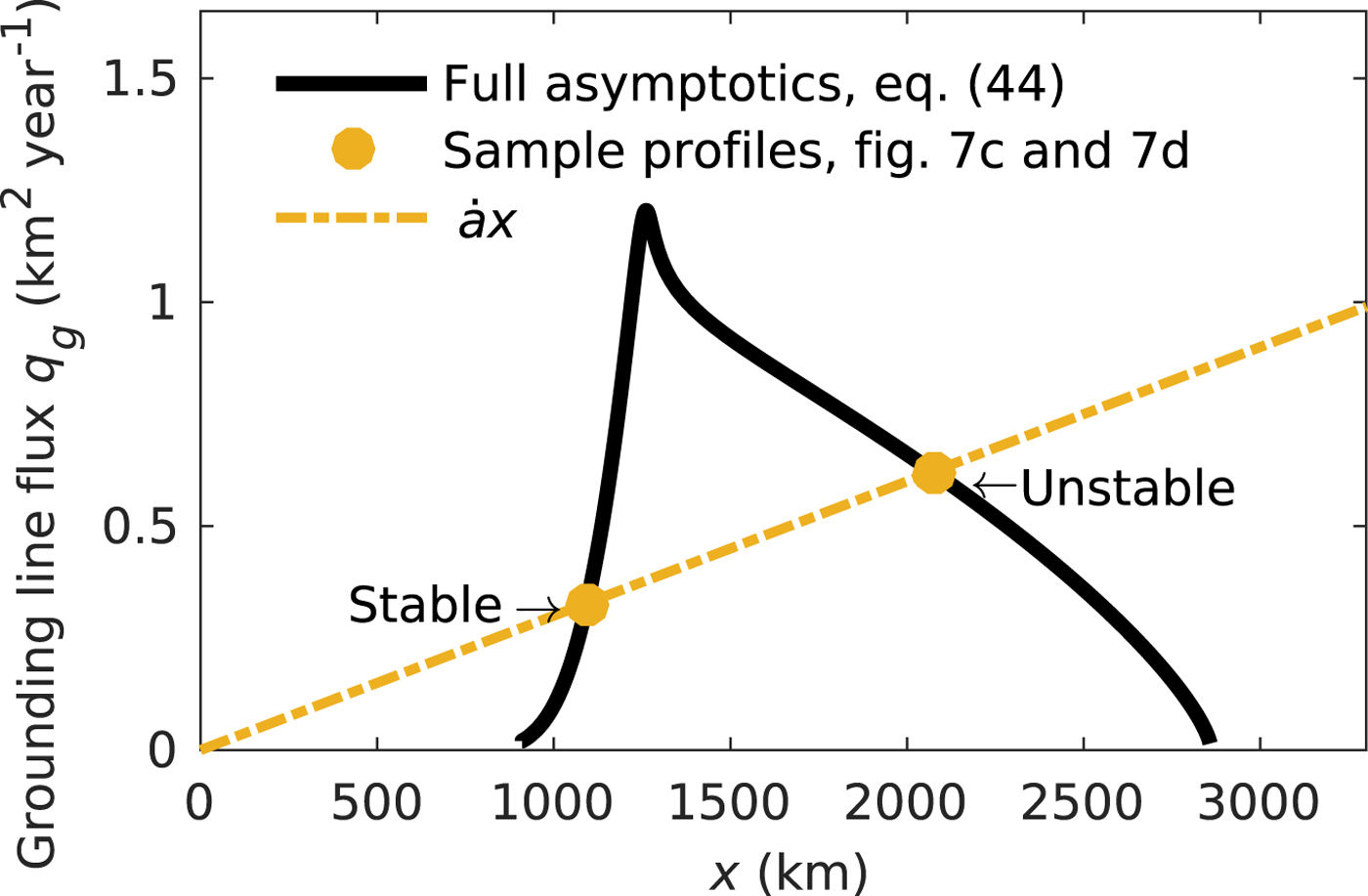
Comparison of Fig. 7d with Figs 5c, 6c illustrates that in the presence of buttressing, different calving laws lead to very different grounding line dynamics. Each of these panels shows ice-sheet profiles at an ice-shelf width of W = 150 km, with stable grounding line positions located at x _g ≈ 1000, x _g ≈ 2000, and x _g ≈ 2800 km, and an unstable grounding line position located at x _g ≈ 2100 km.