


1 Introduction
1.1 Motivation
The theory of the classical theta operator was instrumental in the proof of the weight part of Serre’s modularity conjecture of [Reference Edixhoven14]. Edixhoven’s proof relied, in particular, on the study of the
 $\theta $
-cycles of Tate and Jochnowitz, introduced in [Reference Jochnowitz26]. Since then, much work has been devoted to extending the construction of this operator to other Shimura varieties, with an eye toward generalizations of Serre’s conjecture, or to gain insight in the Langlands programme
$\theta $
-cycles of Tate and Jochnowitz, introduced in [Reference Jochnowitz26]. Since then, much work has been devoted to extending the construction of this operator to other Shimura varieties, with an eye toward generalizations of Serre’s conjecture, or to gain insight in the Langlands programme
 $({\mathrm {mod}}\,p)$
in a broader sense.
$({\mathrm {mod}}\,p)$
in a broader sense.
Interesting results have been obtained in the case of Hilbert modular varieties, starting with the work of Katz, in [Reference Katz31]. Following Katz’s construction of partial Hasse invariants, Andreatta and Goren, in [Reference Andreatta and Goren2], constructed partial theta operators and described their kernels and effects on the weight filtration. These results have subsequently been improved upon and generalized further (see, for instance, [Reference Diamond13]).
In [Reference Yamauchi40], Yamauchi constructed theta operators for Siegel modular forms, in degree
 $2$
, and managed to study their theta cycles.
$2$
, and managed to study their theta cycles.
In [Reference de Shalit and Goren9], de Shalit and Goren, building on their previous work [Reference de Shalit and Goren7], constructed
 $({\mathrm {mod}}\, p)$
and p-adic theta operators on certain unitary Shimura varieties.
$({\mathrm {mod}}\, p)$
and p-adic theta operators on certain unitary Shimura varieties.
At the same time, Eischen, Mantovan, and others, in a series of papers, [Reference Eischen, Flander, Ghitza, Mantovan and McAndrew15–Reference Eischen and Mantovan17], constructed theta operators on PEL Shimura varieties of types A and C. Their approach is independent from that of de Shalit and Goren and it uses geometric techniques which, unlike the more classical theory, do not rely on q-expansions, or more general Fourier–Jacobi and Serre–Tate expansions.
Most of these works leave the problem of studying theta cycles largely open and, where results are obtained, they seem to depend on the specific context. We believe that, in order to understand theta cycles in greater generality, one could benefit from considering new theta or “theta-like” operators, which produce more general weight shifts. Our goal is to present the construction of a new class of generalized theta operators that seem to produce exactly the weight shifts that one would expect from a representation-theoretic viewpoint. Our theory of generalized theta operators ties in neatly with the theory of generalized Hasse invariants of [Reference Boxer5, Reference Goldring and Koskivirta21].
1.2 Notations and conventions
We fix E a quadratic imaginary extension of
 ${\mathbb Q}$
and p an odd, rational prime, split in E. We write
${\mathbb Q}$
and p an odd, rational prime, split in E. We write
 ${\mathbb {F}}$
for a given algebraic closure of
${\mathbb {F}}$
for a given algebraic closure of
 ${\mathbb {F}}_p$
. We choose, once and for all, a preferred embedding
${\mathbb {F}}_p$
. We choose, once and for all, a preferred embedding
 $\sigma \colon E \to {\mathbb C}$
, so that
$\sigma \colon E \to {\mathbb C}$
, so that
 ${\mathrm {Hom}}(E, {\mathbb C}) = \{\sigma , \overline {\sigma }\}$
, and an element
${\mathrm {Hom}}(E, {\mathbb C}) = \{\sigma , \overline {\sigma }\}$
, and an element
 $i = \sqrt {-1} \in {\mathbb C}$
. Let
$i = \sqrt {-1} \in {\mathbb C}$
. Let
 $\delta _{E/{\mathbb Q}}$
denote the unique generator of the different ideal
$\delta _{E/{\mathbb Q}}$
denote the unique generator of the different ideal
 $\mathfrak {D}_{E/{\mathbb Q}}$
with positive imaginary part (with respect to our choices of
$\mathfrak {D}_{E/{\mathbb Q}}$
with positive imaginary part (with respect to our choices of
 $\sigma $
and i). In particular, we have the discriminant
$\sigma $
and i). In particular, we have the discriminant
 $D = D_{E/{\mathbb Q}} = -{\mathrm {N}}_{E/{\mathbb Q}}(\delta _{E/{\mathbb Q}}) = -\delta _{E/{\mathbb Q}} \overline {\delta }_{E/{\mathbb Q}} = -\lvert \delta _{E/{\mathbb Q}} \rvert ^2$
. If we also fix an isomorphism
$D = D_{E/{\mathbb Q}} = -{\mathrm {N}}_{E/{\mathbb Q}}(\delta _{E/{\mathbb Q}}) = -\delta _{E/{\mathbb Q}} \overline {\delta }_{E/{\mathbb Q}} = -\lvert \delta _{E/{\mathbb Q}} \rvert ^2$
. If we also fix an isomorphism
 ${\mathbb C} \cong \overline {{\mathbb Q}}_p$
, we obtain
${\mathbb C} \cong \overline {{\mathbb Q}}_p$
, we obtain
 $$\begin{align*}{\mathrm{Hom}}(E, {\mathbb C}) \cong {\mathrm{Hom}}(E, \overline{{\mathbb Q}}_p) \cong {\mathrm{Hom}}({\mathcal O_E}, {\mathcal{O}}^{\mathrm{ur}}_{\overline{{\mathbb Q}}_p}) \cong {\mathrm{Hom}}({\mathcal O_E}/(p), {\mathbb{F}}), \end{align*}$$
the last two isomorphisms depending on the fact that p is unramified in
 ${\mathcal O_E}$
. The last identification induces on
${\mathcal O_E}$
. The last identification induces on
 $\{\sigma , \overline {\sigma }\}$
an action of the Frobenius automorphism
$\{\sigma , \overline {\sigma }\}$
an action of the Frobenius automorphism
 ${\mathbb {F}}\to {\mathbb {F}}$
by post-composition. Since p is split, this action is trivial. We also write
${\mathbb {F}}\to {\mathbb {F}}$
by post-composition. Since p is split, this action is trivial. We also write
 ${\mathcal {O}}_{E, {\mathrm {ur}}} {:=}q {\mathcal O_E}[1/2D]$
. We fix
${\mathcal {O}}_{E, {\mathrm {ur}}} {:=}q {\mathcal O_E}[1/2D]$
. We fix
 $n\geq 3$
an integer, which will denote throughout the article the relative dimension of the abelian schemes parameterized by the moduli spaces under consideration.
$n\geq 3$
an integer, which will denote throughout the article the relative dimension of the abelian schemes parameterized by the moduli spaces under consideration.
Unless otherwise specified, we assume that all the schemes we work with are locally Noetherian.
1.3 The elliptic case
We sketch here the construction of the theta operator in the classical case of modular curves, following [Reference Katz30]. This construction is the prototype on which most generalizations are based.
Let
 $N \geq 5$
be an integer prime to p. Let
$N \geq 5$
be an integer prime to p. Let
 $Y_1(N)$
, or simply Y, be the modular curve of level
$Y_1(N)$
, or simply Y, be the modular curve of level
 $\Gamma _1(N)$
over
$\Gamma _1(N)$
over
 ${\mathbb {F}}$
. It is a smooth, affine, connected curve over
${\mathbb {F}}$
. It is a smooth, affine, connected curve over
 ${\mathbb {F}}$
, which comes equipped with a universal elliptic curve
${\mathbb {F}}$
, which comes equipped with a universal elliptic curve
 $\pi \colon {\mathcal {E}} \to Y_1(N)$
. From this universal object, we obtain the invertible sheaf
$\pi \colon {\mathcal {E}} \to Y_1(N)$
. From this universal object, we obtain the invertible sheaf
 ${\underline {\omega }} = \pi _\ast \big ( \Omega ^1_{{{\mathcal {E}}}/Y} \big )$
, the so-called Hodge sheaf. One can consider a projective compactification
${\underline {\omega }} = \pi _\ast \big ( \Omega ^1_{{{\mathcal {E}}}/Y} \big )$
, the so-called Hodge sheaf. One can consider a projective compactification
 $Y_1(N) \subset X_1(N)$
, which we simply denote by X, and extend
$Y_1(N) \subset X_1(N)$
, which we simply denote by X, and extend
 ${\underline {\omega }}$
to X (see, for instance, [Reference Deligne and Rapoport12]).
${\underline {\omega }}$
to X (see, for instance, [Reference Deligne and Rapoport12]).
In this setting, modular forms with coefficients in
 ${\mathbb {F}}$
are the elements of the graded
${\mathbb {F}}$
are the elements of the graded
 ${\mathbb {F}}$
-algebra
${\mathbb {F}}$
-algebra
 ${\mathrm {M}}(N)=\oplus _k {\mathrm {M}}_k(N)$
, with
${\mathrm {M}}(N)=\oplus _k {\mathrm {M}}_k(N)$
, with
 ${\mathrm {M}}_k(N) {:=}q H^0(X, {\underline {\omega }}^k)$
. The space of cusp forms of weight k is
${\mathrm {M}}_k(N) {:=}q H^0(X, {\underline {\omega }}^k)$
. The space of cusp forms of weight k is
 ${\mathrm {S}}_k(N) {:=}q H^0(X, {\underline {\omega }}^k(-C)) \subseteq M_k(N)$
, where
${\mathrm {S}}_k(N) {:=}q H^0(X, {\underline {\omega }}^k(-C)) \subseteq M_k(N)$
, where
 $C = X \setminus Y$
is the cuspidal divisor. On this algebra, one can define as usual an action of the Hecke operators
$C = X \setminus Y$
is the cuspidal divisor. On this algebra, one can define as usual an action of the Hecke operators
 $T_l$
, for
$T_l$
, for
 $l \neq p$
any prime, and hence an action of the Hecke algebra they generate.
$l \neq p$
any prime, and hence an action of the Hecke algebra they generate.
Since we are working in characteristic p, over Y, we can consider the Verschiebung morphism
 $V \colon {\mathcal {E}}^{(p)} \to {\mathcal {E}}$
, which by pullback defines
$V \colon {\mathcal {E}}^{(p)} \to {\mathcal {E}}$
, which by pullback defines
 $V \colon {\underline {\omega }} \to {\underline {\omega }}^{(p)} \cong {\underline {\omega }}^p$
and hence a section
$V \colon {\underline {\omega }} \to {\underline {\omega }}^{(p)} \cong {\underline {\omega }}^p$
and hence a section
 $h \in H^0(Y, {\underline {\omega }}^{p-1})$
. This section extends to a form
$h \in H^0(Y, {\underline {\omega }}^{p-1})$
. This section extends to a form
 $h \in M_{p-1}(N)$
, which is called the Hasse invariant. It vanishes with simple zeros precisely at the supersingular points
$h \in M_{p-1}(N)$
, which is called the Hasse invariant. It vanishes with simple zeros precisely at the supersingular points
 $Y^{\mathrm {ss}} \subset Y \subset X$
and its q-expansion at the cusps is identically
$Y^{\mathrm {ss}} \subset Y \subset X$
and its q-expansion at the cusps is identically
 $1$
. The complement
$1$
. The complement
 $Y^{\mathrm {ord}} = Y \setminus Y^{\mathrm {ss}}$
, called the ordinary locus, is a dense open subset of Y.
$Y^{\mathrm {ord}} = Y \setminus Y^{\mathrm {ss}}$
, called the ordinary locus, is a dense open subset of Y.
A key observation in Katz’s geometric construction of the classical theta operator is that, over the ordinary locus, there is a natural splitting of the Hodge filtration
 $$ \begin{align} 0 \longrightarrow {\underline{\omega}} \longrightarrow H^1_{\mathrm{dR}}({\mathcal{E}}/Y) \longrightarrow {\underline{\omega}}^\vee \longrightarrow 0. \end{align} $$
Write
 $H = H^1_{\mathrm {dR}}({\mathcal {E}}/Y) = R^1\pi _\ast \Omega ^{\bullet }_{{\mathcal {E}}/Y}$
for the (relative) de Rham cohomology of
$H = H^1_{\mathrm {dR}}({\mathcal {E}}/Y) = R^1\pi _\ast \Omega ^{\bullet }_{{\mathcal {E}}/Y}$
for the (relative) de Rham cohomology of
 $\pi $
. Let
$\pi $
. Let
 $F \colon H^{(p)} \to H$
be the morphism obtained by pulling back via the relative Frobenius
$F \colon H^{(p)} \to H$
be the morphism obtained by pulling back via the relative Frobenius
 $F \colon {\mathcal {E}} \to {\mathcal {E}}^{(p)}$
. Katz shows that, over
$F \colon {\mathcal {E}} \to {\mathcal {E}}^{(p)}$
. Katz shows that, over
 $Y^{\mathrm {ord}}$
,
$Y^{\mathrm {ord}}$
,
 ${\mathcal {U}} = {{\mathrm {im}}}(F)$
is a complement of the subsheaf
${\mathcal {U}} = {{\mathrm {im}}}(F)$
is a complement of the subsheaf
 ${\underline {\omega }} \subset H$
, providing
${\underline {\omega }} \subset H$
, providing
 $H \cong {\underline {\omega }} \oplus {\mathcal {U}},$
which is called the unit-root splitting (of (H)). While this splitting cannot be naturally extended to Y, the projection parallel to it,
$H \cong {\underline {\omega }} \oplus {\mathcal {U}},$
which is called the unit-root splitting (of (H)). While this splitting cannot be naturally extended to Y, the projection parallel to it,
 $p_{\mathrm {ur}} \colon H \to {\underline {\omega }},$
does extend to Y upon multiplication by the Hasse invariant. This underlies Katz’s construction of the theta operator. We present here a reformulation of these facts which leads naturally to the generalizations we want to discuss. The open
$p_{\mathrm {ur}} \colon H \to {\underline {\omega }},$
does extend to Y upon multiplication by the Hasse invariant. This underlies Katz’s construction of the theta operator. We present here a reformulation of these facts which leads naturally to the generalizations we want to discuss. The open
 $Y^{\mathrm {ord}}$
is the locus where
$Y^{\mathrm {ord}}$
is the locus where
 $V|_{\underline {\omega }} \colon {\underline {\omega }} \to {\underline {\omega }}^{(p)}$
is an isomorphism. Thus, on
$V|_{\underline {\omega }} \colon {\underline {\omega }} \to {\underline {\omega }}^{(p)}$
is an isomorphism. Thus, on
 $Y^{\mathrm {ord}}$
, we may consider the composition
$Y^{\mathrm {ord}}$
, we may consider the composition
 $$ \begin{align} H \overset{V}{\longrightarrow} {\underline{\omega}}^{(p)} \overset{V|_{{\underline{\omega}}}^{-1}}{\longrightarrow} {\underline{\omega}}. \end{align} $$
It is easy to see that the map
 $H \to {\underline {\omega }}$
from (P) is precisely
$H \to {\underline {\omega }}$
from (P) is precisely
 $p_{\mathrm {ur}}$
. In particular, the morphism
$p_{\mathrm {ur}}$
. In particular, the morphism
 $h \cdot p_{\mathrm {ur}} \colon H \to {\underline {\omega }}^p$
can be written as
$h \cdot p_{\mathrm {ur}} \colon H \to {\underline {\omega }}^p$
can be written as
 $$ \begin{align} H \overset{V}{\longrightarrow} {\underline{\omega}}^{p} \overset{V|_{{\underline{\omega}}}^{-1}}{\longrightarrow} {\underline{\omega}} \overset{h = V|_{{\underline{\omega}}}}{\longrightarrow} {\underline{\omega}}^p, \end{align} $$
which is simply the surjection
 $V \colon H \to {\underline {\omega }}^p$
and extends from
$V \colon H \to {\underline {\omega }}^p$
and extends from
 $Y^{\mathrm {ord}}$
to the entire modular curve. More generally, one can look at
$Y^{\mathrm {ord}}$
to the entire modular curve. More generally, one can look at
 ${\mathrm {Sym}}^k(p_{\mathrm {ur}}),$
where
${\mathrm {Sym}}^k(p_{\mathrm {ur}}),$
where
 ${\mathrm {Sym}}^k$
is the k-th symmetric power. The locally free sheaf
${\mathrm {Sym}}^k$
is the k-th symmetric power. The locally free sheaf
 ${\mathrm {Sym}}^k(H)$
admits a descending filtration
${\mathrm {Sym}}^k(H)$
admits a descending filtration
 $F^i({\mathrm {Sym}}^k(H))$
, afforded by (H), and one can show that the morphism
$F^i({\mathrm {Sym}}^k(H))$
, afforded by (H), and one can show that the morphism
 $$ \begin{align*} h \cdot {\mathrm{Sym}}^k(p_{\mathrm{ur}})|_{F^{k-1}({\mathrm{Sym}}^k H)} \colon F^{k-1}({\mathrm{Sym}}^k H) \to {\underline{\omega}}^{k+p-1} \end{align*} $$
extends from
 $Y^{\mathrm {ord}}$
to Y. This is important, because on
$Y^{\mathrm {ord}}$
to Y. This is important, because on
 ${\mathrm {Sym}}^k(H)$
and over Y, one can define the Gauss–Manin connection
${\mathrm {Sym}}^k(H)$
and over Y, one can define the Gauss–Manin connection
 $$ \begin{align*} \nabla \colon {\mathrm{Sym}}^k(H) \longrightarrow {\mathrm{Sym}}^k(H) \otimes \Omega^1_{Y/{\mathbb{F}}}, \end{align*} $$
which satisfies a general transversality property that implies
 $\nabla ({\underline {\omega }}^k) \subseteq F^{k-1}({\mathrm {Sym}}^k(H)) \otimes \Omega ^1_{Y/{\mathbb {F}}}.$
All of this is used by Katz to define the theta operator as the composition
$\nabla ({\underline {\omega }}^k) \subseteq F^{k-1}({\mathrm {Sym}}^k(H)) \otimes \Omega ^1_{Y/{\mathbb {F}}}.$
All of this is used by Katz to define the theta operator as the composition
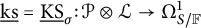
 $$ \begin{align*} \theta \colon {\underline{\omega}}^k \xrightarrow{\nabla} F^{k-1}({\mathrm{Sym}}^k(H)) \otimes \Omega^1_{Y/{\mathbb{F}}} \xrightarrow{(h \cdot {\mathrm{Sym}}^k(p_{\mathrm{ur}})) \otimes {\underline{{\mathrm{ks}}}}^{-1}} {\underline{\omega}}^{k+p+1}, \end{align*} $$
where
 ${\underline {{\mathrm {ks}}}} \colon {\underline {\omega }}^2 \to \Omega ^1_{Y/{\mathbb {F}}} $
is the Kodaira–Spencer isomorphism. A more detailed inspection of
${\underline {{\mathrm {ks}}}} \colon {\underline {\omega }}^2 \to \Omega ^1_{Y/{\mathbb {F}}} $
is the Kodaira–Spencer isomorphism. A more detailed inspection of
 $\theta $
, for instance, via q-expansions and the q-expansion principle, shows that it extends to an operator over X. Taking global sections gives rise to
$\theta $
, for instance, via q-expansions and the q-expansion principle, shows that it extends to an operator over X. Taking global sections gives rise to
 $\theta \colon {\mathrm {M}}_k(N) \to {\mathrm {S}}_{k+p+1}(N), $
the theta operator on modular forms. This is a derivation of the algebra
$\theta \colon {\mathrm {M}}_k(N) \to {\mathrm {S}}_{k+p+1}(N), $
the theta operator on modular forms. This is a derivation of the algebra
 ${\mathrm {M}}(N)$
of modular forms of degree
${\mathrm {M}}(N)$
of modular forms of degree
 $p+1$
. By this, we mean that for two modular forms
$p+1$
. By this, we mean that for two modular forms
 $f, g$
, we have
$f, g$
, we have
 $\theta (fg) = f\theta (g) + \theta (f)g$
, which is a cusp form of degree
$\theta (fg) = f\theta (g) + \theta (f)g$
, which is a cusp form of degree
 $p+1+\deg (fg)$
. The operator
$p+1+\deg (fg)$
. The operator
 $\theta $
is h-linear, in the sense that
$\theta $
is h-linear, in the sense that
 $\theta (h) = 0$
. Moreover, one can show that
$\theta (h) = 0$
. Moreover, one can show that
 $T_l \, \theta = l\, \theta \, T_l.$
In particular, if f is an eigenform, so is
$T_l \, \theta = l\, \theta \, T_l.$
In particular, if f is an eigenform, so is
 $\theta (f)$
.
$\theta (f)$
.
1.4 The Picard case
We briefly sketch the construction of ordinary and generalized theta operators in the special case of Picard modular surfaces to illustrate the main ideas involved.
First, let us set up some notation. Write S for the geometric special fiber of the Picard modular surface over
 ${\mathbb {F}}$
with some neat, p-hyperspecial level. Roughly speaking, this is a moduli space of polarized abelian schemes of relative dimension
${\mathbb {F}}$
with some neat, p-hyperspecial level. Roughly speaking, this is a moduli space of polarized abelian schemes of relative dimension
 $3$
endowed with an action of
$3$
endowed with an action of
 $\mathcal {O}_E$
, the ring of integers of E. For more details on the moduli problem, see the next section. We have a universal object
$\mathcal {O}_E$
, the ring of integers of E. For more details on the moduli problem, see the next section. We have a universal object
 $\pi \colon A \to S$
and, as before, we can consider the Hodge sheaf
$\pi \colon A \to S$
and, as before, we can consider the Hodge sheaf
 ${\underline {\omega }} = \pi _\ast (\Omega ^1_{A/S})$
. In this case,
${\underline {\omega }} = \pi _\ast (\Omega ^1_{A/S})$
. In this case,
 ${\underline {\omega }}$
is locally free of rank
${\underline {\omega }}$
is locally free of rank
 $3$
and, under the induced action of
$3$
and, under the induced action of
 ${\mathcal {O}}_E$
, it decomposes into the direct sum of two locally free sheaves
${\mathcal {O}}_E$
, it decomposes into the direct sum of two locally free sheaves
 $\mathcal {P} = {\underline {\omega }}_\sigma $
and
$\mathcal {P} = {\underline {\omega }}_\sigma $
and
 $\mathcal {L} = {\underline {\omega }}_{\overline {\sigma }}$
, the subscripts indicating that
$\mathcal {L} = {\underline {\omega }}_{\overline {\sigma }}$
, the subscripts indicating that
 ${\mathcal {O}}_E$
acts on
${\mathcal {O}}_E$
acts on
 ${\underline {\omega }}_\tau $
via
${\underline {\omega }}_\tau $
via
 $\tau \in \{\sigma , \overline {\sigma }\}$
. We assume that
$\tau \in \{\sigma , \overline {\sigma }\}$
. We assume that
 ${\mathcal {P}}$
and
${\mathcal {P}}$
and
 ${\mathcal {L}}$
have ranks
${\mathcal {L}}$
have ranks
 $2$
and
$2$
and
 $1$
, respectively. We also consider the sheaf
$1$
, respectively. We also consider the sheaf
 $\delta = \delta _\sigma \cong \det {\mathcal {P}} \otimes {\mathcal {L}}^{-1}$
. We write
$\delta = \delta _\sigma \cong \det {\mathcal {P}} \otimes {\mathcal {L}}^{-1}$
. We write
 $S^\mu \subseteq S$
for the ordinary locus, the maximal stratum in the Ekedahl–Oort stratification of S, which is a dense open in S. The complement
$S^\mu \subseteq S$
for the ordinary locus, the maximal stratum in the Ekedahl–Oort stratification of S, which is a dense open in S. The complement
 $S^{\mathrm {no}} = S \setminus S^\mu $
is called the non-ordinary locus and is given by the disjoint union of the almost ordinary locus
$S^{\mathrm {no}} = S \setminus S^\mu $
is called the non-ordinary locus and is given by the disjoint union of the almost ordinary locus
 $S^{\mathrm {ao}}$
, the EO stratum of dimension 1, and the core locus
$S^{\mathrm {ao}}$
, the EO stratum of dimension 1, and the core locus
 $S^{\mathrm {core}}$
, the EO stratum of dimension
$S^{\mathrm {core}}$
, the EO stratum of dimension
 $0$
. We define an automorphic weight to be a couple
$0$
. We define an automorphic weight to be a couple
 $({\underline {k}}, w)$
, where
$({\underline {k}}, w)$
, where
 ${\underline {k}}=(k_1 \geq k_2) \in {\mathbb Z}^2$
,
${\underline {k}}=(k_1 \geq k_2) \in {\mathbb Z}^2$
,
 $w \in {\mathbb Z}$
, and the corresponding automorphic sheaf to be
$w \in {\mathbb Z}$
, and the corresponding automorphic sheaf to be
 $$\begin{align*}{\underline{\omega}}^{{\underline{k}}, w} {:=}q {\mathrm{Sym}}^{k_1-k_2}({\mathcal{P}}) \otimes \det({\mathcal{P}})^{k_2} \otimes \delta^w. \end{align*}$$
Analogously to (H), we have a Hodge filtration on
 $H = H^1_{\mathrm {dR}}(A/S)$
, of which we can take components according to the action of E:
$H = H^1_{\mathrm {dR}}(A/S)$
, of which we can take components according to the action of E:
 $$ \begin{align} 0 \longrightarrow {\mathcal{P}} \longrightarrow &H_\sigma \longrightarrow {\mathcal{L}}^\vee \longrightarrow 0, \end{align} $$
 $$ \begin{align} 0 \longrightarrow {\mathcal{L}} \longrightarrow &H_{\overline{\sigma}} \longrightarrow {\mathcal{P}}^\vee \longrightarrow 0. \end{align} $$
Katz’s explicit construction of the unit-root splitting in the elliptic case carries over and provides a natural splitting of (HP) and (HL) over
 $S^\mu $
. Like in Section 1.3, we may reinterpret this unit-root splitting in terms of the Verschiebung morphism. Let
$S^\mu $
. Like in Section 1.3, we may reinterpret this unit-root splitting in terms of the Verschiebung morphism. Let
 $V \colon H \to H^{(p)}$
be the pullback of the Verschiebung morphism of the universal abelian scheme
$V \colon H \to H^{(p)}$
be the pullback of the Verschiebung morphism of the universal abelian scheme
 $A \to S$
. We consider its CM components
$A \to S$
. We consider its CM components
 $V_\sigma \colon H_\sigma \to H_\sigma ^{(p)}, V_{\overline {\sigma }} \colon H_{\overline {\sigma }} \to H_{\overline {\sigma }}^{(p)}$
, whose images are
$V_\sigma \colon H_\sigma \to H_\sigma ^{(p)}, V_{\overline {\sigma }} \colon H_{\overline {\sigma }} \to H_{\overline {\sigma }}^{(p)}$
, whose images are
 ${\mathcal {P}}^{(p)}, {\mathcal {L}}^p$
, respectively. Over
${\mathcal {P}}^{(p)}, {\mathcal {L}}^p$
, respectively. Over
 $S^\mu $
, the restrictions
$S^\mu $
, the restrictions
 $V_\sigma |_{\mathcal {P}} \colon {\mathcal {P}} \to {\mathcal {P}}^{(p)}$
,
$V_\sigma |_{\mathcal {P}} \colon {\mathcal {P}} \to {\mathcal {P}}^{(p)}$
,
 $V_{\overline {\sigma }}|_{\mathcal {L}} \colon {\mathcal {L}} \to {\mathcal {L}}^p$
are isomorphisms and we can use them to define
$V_{\overline {\sigma }}|_{\mathcal {L}} \colon {\mathcal {L}} \to {\mathcal {L}}^p$
are isomorphisms and we can use them to define
 $$\begin{align*}p_{{\mathrm{ur}}, \sigma}\colon {H}_\sigma \xrightarrow{V_\sigma} {\mathcal{P}}^{(p)} \xrightarrow{V_\sigma|_{{\mathcal{P}}}^{-1}} {\mathcal{P}}, \,p_{{\mathrm{ur}}, {\overline{\sigma}}}\colon {H}_{\overline \sigma} \xrightarrow{V_{\overline{\sigma}}} {\mathcal{L}}^{p} \xrightarrow{V_{\overline{\sigma}}|_{{\mathcal{L}}}^{-1}} {\mathcal{L}}. \end{align*}$$
These morphisms give the unit-root splitting in this case. Like in the classical case, we cannot extend this splitting naturally to the non-ordinary locus
 $S^{\mathrm {no}} = S \setminus S^\mu $
, essentially because
$S^{\mathrm {no}} = S \setminus S^\mu $
, essentially because
 $V \colon {\underline {\omega }} \to {\underline {\omega }}^{(p)}$
is not invertible on
$V \colon {\underline {\omega }} \to {\underline {\omega }}^{(p)}$
is not invertible on
 $S^{\mathrm {no}}$
, but we can use the Hasse invariant to clear this obstruction. In this case, the Hasse invariant is the section
$S^{\mathrm {no}}$
, but we can use the Hasse invariant to clear this obstruction. In this case, the Hasse invariant is the section
 $h \in H^0(S, (\det {\underline {\omega }})^{p-1})$
, which is obtained as the determinant of the morphism
$h \in H^0(S, (\det {\underline {\omega }})^{p-1})$
, which is obtained as the determinant of the morphism
 $V\colon {\underline {\omega }} \to {\underline {\omega }}^{(p)}$
. The section h is nowhere-vanishing on
$V\colon {\underline {\omega }} \to {\underline {\omega }}^{(p)}$
. The section h is nowhere-vanishing on
 $S^\mu $
, identically
$S^\mu $
, identically
 $0$
on
$0$
on
 $S^{\mathrm {no}}$
and it splits as the product
$S^{\mathrm {no}}$
and it splits as the product
 $h = h_\sigma \cdot h_{\overline {\sigma }}$
, where
$h = h_\sigma \cdot h_{\overline {\sigma }}$
, where
 $h_\sigma \in H^0(S, (\det {\mathcal {P}})^{p-1}), h_{\overline {\sigma }} \in H^0(S, {\mathcal {L}}^{p-1}),$
are obtained from
$h_\sigma \in H^0(S, (\det {\mathcal {P}})^{p-1}), h_{\overline {\sigma }} \in H^0(S, {\mathcal {L}}^{p-1}),$
are obtained from
 $\det V_\sigma $
and
$\det V_\sigma $
and
 $V_{\overline {\sigma }}$
, respectively. Both
$V_{\overline {\sigma }}$
, respectively. Both
 $h_\sigma $
and
$h_\sigma $
and
 $h_{\overline {\sigma }}$
vanish with simple zeros on
$h_{\overline {\sigma }}$
vanish with simple zeros on
 $S^{\mathrm {no}}$
. Just like in the elliptic case, the morphism
$S^{\mathrm {no}}$
. Just like in the elliptic case, the morphism
 $h_{\overline {\sigma }} \cdot p_{{\mathrm {ur}}, \overline {\sigma }} \colon H_{\overline {\sigma }} \to {\mathcal {L}}^p$
can be extended from
$h_{\overline {\sigma }} \cdot p_{{\mathrm {ur}}, \overline {\sigma }} \colon H_{\overline {\sigma }} \to {\mathcal {L}}^p$
can be extended from
 $S^\mu $
to S, since it simply coincides with
$S^\mu $
to S, since it simply coincides with
 $V\colon H_{\overline {\sigma }} \to {\mathcal {L}}^p$
. We can also extend
$V\colon H_{\overline {\sigma }} \to {\mathcal {L}}^p$
. We can also extend
 $$\begin{align*}h_\sigma \cdot p_{{\mathrm{ur}}, \sigma} \colon H_\sigma \to {\mathcal{P}} \otimes (\det {\mathcal{P}})^{p-1} \end{align*}$$
from
 $S^\mu $
to S, even if the rank of
$S^\mu $
to S, even if the rank of
 ${\mathcal {P}}$
is greater than
${\mathcal {P}}$
is greater than
 $1$
. In fact, the product
$1$
. In fact, the product
 $h_\sigma \cdot V^{-1} \colon {\mathcal {P}}^{(p)} \to {\mathcal {P}} \otimes (\det {\mathcal {P}})^{p-1}$
is the adjugate
$h_\sigma \cdot V^{-1} \colon {\mathcal {P}}^{(p)} \to {\mathcal {P}} \otimes (\det {\mathcal {P}})^{p-1}$
is the adjugate
 $V^{\mathrm {adj}}$
, of the morphism
$V^{\mathrm {adj}}$
, of the morphism
 $V \colon {\mathcal {P}} \to {\mathcal {P}}^{(p)}$
which, like V, is defined on the whole of S. As a result, the extension of
$V \colon {\mathcal {P}} \to {\mathcal {P}}^{(p)}$
which, like V, is defined on the whole of S. As a result, the extension of
 $h_\sigma \cdot p_{{\mathrm {ur}}, \sigma }$
is the composition
$h_\sigma \cdot p_{{\mathrm {ur}}, \sigma }$
is the composition
 $V|_{{\mathcal {P}}}^{\mathrm {adj}} \circ V \colon H_\sigma \to {\mathcal {P}} \otimes (\det {\mathcal {P}})^{p-1}.$
Considering
$V|_{{\mathcal {P}}}^{\mathrm {adj}} \circ V \colon H_\sigma \to {\mathcal {P}} \otimes (\det {\mathcal {P}})^{p-1}.$
Considering
 $V^{\mathrm {adj}}$
is a key idea of [Reference Eischen, Flander, Ghitza, Mantovan and McAndrew15]. In Lemma 6.1, we prove a general result for extending morphisms from
$V^{\mathrm {adj}}$
is a key idea of [Reference Eischen, Flander, Ghitza, Mantovan and McAndrew15]. In Lemma 6.1, we prove a general result for extending morphisms from
 $S^\mu $
to S, which allows us to consider the correct analog of the above construction to define the theta operator on
$S^\mu $
to S, which allows us to consider the correct analog of the above construction to define the theta operator on
 ${\underline {\omega }}^{{\underline {k}}, w}$
, for a general weight
${\underline {\omega }}^{{\underline {k}}, w}$
, for a general weight
 $({\underline {k}}, w)$
. Lemma 6.1 is also used crucially in our definition of generalized theta operators. In the Picard case, we define, for
$({\underline {k}}, w)$
. Lemma 6.1 is also used crucially in our definition of generalized theta operators. In the Picard case, we define, for
 $({\underline {k}}, w)$
with
$({\underline {k}}, w)$
with
 $k_2 \geq 0$
, a morphism
$k_2 \geq 0$
, a morphism
 $h_\sigma \cdot (p_{{\mathrm {ur}}})^{{\underline {k}}, w} \colon H^{{\underline {k}}, w} \to {\underline {\omega }}^{{\underline {k}}, w} \otimes (\det {\mathcal {P}})^{p-1}$
, where
$h_\sigma \cdot (p_{{\mathrm {ur}}})^{{\underline {k}}, w} \colon H^{{\underline {k}}, w} \to {\underline {\omega }}^{{\underline {k}}, w} \otimes (\det {\mathcal {P}})^{p-1}$
, where
 $$ \begin{align*} h_\sigma \cdot (p_{{\mathrm{ur}}})^{{\underline{k}}, w} &= h_\sigma \cdot {\mathrm{Sym}}^{k_1-k_2}(p_{{\mathrm{ur}}, \sigma}) \otimes {\mathrm{Sym}}^{k_2}(\wedge^2(p_{{\mathrm{ur}}, \sigma})) \otimes {\mathrm{id}}_\delta, \\ H^{{\underline{k}}, w} &= {\mathrm{Sym}}^{k_1-k_2}(H_\sigma) \otimes {\mathrm{Sym}}^{k_2}(\wedge^2(H_\sigma)) \otimes \delta. \end{align*} $$
While
 $h_\sigma \cdot (p_{{\mathrm {ur}}})^{{\underline {k}}, w}$
itself does not extend from
$h_\sigma \cdot (p_{{\mathrm {ur}}})^{{\underline {k}}, w}$
itself does not extend from
 $S^\mu $
to S, a relevant restriction of this morphism does, by Lemma 6.1.
$S^\mu $
to S, a relevant restriction of this morphism does, by Lemma 6.1.
As in the elliptic case, we have natural filtrations
 ${\mathcal {P}} \subset H_\sigma $
and
${\mathcal {P}} \subset H_\sigma $
and
 ${\mathcal {L}} \subset H_{\overline {\sigma }}$
, with respect to which the Gauss–Manin connection
${\mathcal {L}} \subset H_{\overline {\sigma }}$
, with respect to which the Gauss–Manin connection
 $\nabla \colon H \to H \otimes \Omega ^1_{S/{\mathbb {F}}}$
satisfies a natural transversality property. Unlike in the classical case, the Kodaira–Spencer morphism
$\nabla \colon H \to H \otimes \Omega ^1_{S/{\mathbb {F}}}$
satisfies a natural transversality property. Unlike in the classical case, the Kodaira–Spencer morphism
 ${\underline {{\mathrm {KS}}}} \colon {\underline {\omega }} \otimes {\underline {\omega }} \to \Omega ^1$
is not an isomorphism, but its restriction
${\underline {{\mathrm {KS}}}} \colon {\underline {\omega }} \otimes {\underline {\omega }} \to \Omega ^1$
is not an isomorphism, but its restriction
 ${\underline {{\mathrm {ks}}}} = {\underline {{\mathrm {KS}}}}_\sigma \colon {\mathcal {P}} \otimes {\mathcal {L}} \to \Omega ^1_{S/{\mathbb {F}}}$
is. With our conventions for the automorphic sheaves, this becomes the isomorphism
${\underline {{\mathrm {ks}}}} = {\underline {{\mathrm {KS}}}}_\sigma \colon {\mathcal {P}} \otimes {\mathcal {L}} \to \Omega ^1_{S/{\mathbb {F}}}$
is. With our conventions for the automorphic sheaves, this becomes the isomorphism
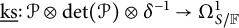 ${\underline {{\mathrm {ks}}}} \colon {\mathcal {P}} \otimes \det ({\mathcal {P}}) \otimes \delta ^{-1} \to \Omega ^1_{S/{\mathbb {F}}}$
. We can use all of this to define the operator
${\underline {{\mathrm {ks}}}} \colon {\mathcal {P}} \otimes \det ({\mathcal {P}}) \otimes \delta ^{-1} \to \Omega ^1_{S/{\mathbb {F}}}$
. We can use all of this to define the operator
 $\theta _1 $
as the following composition:
$\theta _1 $
as the following composition:
 $$ \begin{align*} \theta_1 \colon {\underline{\omega}}^{{\underline{k}}, w} \overset{\nabla}{\longrightarrow}H^{{\underline{k}}, w} \otimes \Omega^1_{S/{\mathbb{F}}} \xrightarrow{{\underline{{\mathrm{ks}}}}^{-1}} &H^{{\underline{k}}, w} \otimes {\mathcal{P}} \otimes \det({\mathcal{P}}) \otimes \delta^{-1}\\ \xrightarrow{h_\sigma \cdot (p_{{\mathrm{ur}}})^{{\underline{k}}, w} \otimes {\mathrm{id}}} &{\underline{\omega}} ^{{\underline{k}}, w} \otimes {\mathcal{P}} \otimes \det({\mathcal{P}})^p \otimes \delta^{-1} \longrightarrow {\underline{\omega}}^{{\underline{k}}+(p+1, p), w-1}. \end{align*} $$
This produces a weight shift of the form
 $((p+1, p), -1)$
, that is, mostly in the direction of
$((p+1, p), -1)$
, that is, mostly in the direction of
 $\det {\mathcal {P}} \cong {\mathcal {L}}$
. To obtain a different weight shift, we have to generalize the projection
$\det {\mathcal {P}} \cong {\mathcal {L}}$
. To obtain a different weight shift, we have to generalize the projection
 $h_\sigma \cdot (p_{{\mathrm {ur}}})^{{\underline {k}}, w}$
. This does not seem to be possible on S. To remedy this, in this work, we use the structure theory of the Ekedahl–Oort stratification to obtain such generalizations and construct theta operators on lower strata. Let us discuss some of the ingredients involved in this new construction.
$h_\sigma \cdot (p_{{\mathrm {ur}}})^{{\underline {k}}, w}$
. This does not seem to be possible on S. To remedy this, in this work, we use the structure theory of the Ekedahl–Oort stratification to obtain such generalizations and construct theta operators on lower strata. Let us discuss some of the ingredients involved in this new construction.
On
 $S^{\mathrm {no}}$
, we have a short exact sequence
$S^{\mathrm {no}}$
, we have a short exact sequence
 $$ \begin{align} 0 \longrightarrow \mathcal{P}_0 \longrightarrow \mathcal{P} \longrightarrow \mathcal{P}_\mu \longrightarrow 0, \end{align} $$
where
 ${\mathcal {P}}_0 {:=}q \ker (V_\sigma \colon {\mathcal {P}} \to {\mathcal {P}}^{(p)})$
and the quotient
${\mathcal {P}}_0 {:=}q \ker (V_\sigma \colon {\mathcal {P}} \to {\mathcal {P}}^{(p)})$
and the quotient
 ${\mathcal {P}}_\mu $
are invertible sheaves. Setting
${\mathcal {P}}_\mu $
are invertible sheaves. Setting
 $H_\mu = H_\sigma /{\mathcal {P}}_0$
, we have a short exact sequence on
$H_\mu = H_\sigma /{\mathcal {P}}_0$
, we have a short exact sequence on
 $S^{\mathrm {no}}$
 $$ \begin{align} 0 \longrightarrow {\mathcal{P}}_\mu \longrightarrow H_\mu \longrightarrow {\mathcal{L}}^\vee \longrightarrow 0, \end{align} $$
which is analogous to (HP). By general properties of the GM connection, we have that
 $\nabla ({\mathcal {P}}_0) \subseteq {\mathcal {P}}_0 \otimes \Omega ^1_{S^{\mathrm {no}}/{\mathbb {F}}}$
, which implies that
$\nabla ({\mathcal {P}}_0) \subseteq {\mathcal {P}}_0 \otimes \Omega ^1_{S^{\mathrm {no}}/{\mathbb {F}}}$
, which implies that
 $\nabla $
induces a connection
$\nabla $
induces a connection
 $\nabla \colon H_\mu \to H_\mu \otimes \Omega ^1_{S/{\mathbb {F}}}$
. The Verschiebung morphism induces a map
$\nabla \colon H_\mu \to H_\mu \otimes \Omega ^1_{S/{\mathbb {F}}}$
. The Verschiebung morphism induces a map
 $V \colon H_\mu \to H_\mu ^{(p)}$
, the image of which is
$V \colon H_\mu \to H_\mu ^{(p)}$
, the image of which is
 ${\mathcal {P}}_\mu ^p$
. The almost-ordinary locus
${\mathcal {P}}_\mu ^p$
. The almost-ordinary locus
 $S^{\mathrm {ao}}$
can be characterized as the locus in
$S^{\mathrm {ao}}$
can be characterized as the locus in
 $S^{\mathrm {no}}$
where the restriction
$S^{\mathrm {no}}$
where the restriction
 $V|_{{\mathcal {P}}_\mu } \colon {\mathcal {P}}_\mu \to {\mathcal {P}}_\mu ^p$
is an isomorphism. Hence, we can use an idea similar to our reinterpretation of the unit-root splitting to construct a splitting of (HP'), by defining
$V|_{{\mathcal {P}}_\mu } \colon {\mathcal {P}}_\mu \to {\mathcal {P}}_\mu ^p$
is an isomorphism. Hence, we can use an idea similar to our reinterpretation of the unit-root splitting to construct a splitting of (HP'), by defining
 $$\begin{align*}p_{{\mathrm{ur}}, 2} \colon H_\mu \xrightarrow{V} {\mathcal{P}}_\mu^p \xrightarrow{V|_{{\mathcal{P}}_\mu}^{-1}} {\mathcal{P}}_\mu. \end{align*}$$
We can also consider a partial generalized Hasse invariant
 $A_{2} \in H^0(S^{\mathrm {no}}, {\mathcal {P}}_\mu ^{p-1})$
, corresponding to
$A_{2} \in H^0(S^{\mathrm {no}}, {\mathcal {P}}_\mu ^{p-1})$
, corresponding to
 $V \colon {\mathcal {P}}_\mu \to {\mathcal {P}}_\mu ^p$
. The vanishing locus of
$V \colon {\mathcal {P}}_\mu \to {\mathcal {P}}_\mu ^p$
. The vanishing locus of
 $A_{2}$
is precisely
$A_{2}$
is precisely
 $S^{\mathrm {no}} \setminus S^{\mathrm {ao}}$
, the core locus of S. We can show that while the morphism
$S^{\mathrm {no}} \setminus S^{\mathrm {ao}}$
, the core locus of S. We can show that while the morphism
 $p_{{\mathrm {ur}}, 2}$
does not extend from
$p_{{\mathrm {ur}}, 2}$
does not extend from
 $S^{\mathrm {ao}}$
to
$S^{\mathrm {ao}}$
to
 $S^{\mathrm {no}}$
, the map
$S^{\mathrm {no}}$
, the map
 $A_{2} \cdot p_{{\mathrm {ur}}, 2} \colon H_\mu \to {\mathcal {P}}_\mu ^p$
does. More generally, the morphisms
$A_{2} \cdot p_{{\mathrm {ur}}, 2} \colon H_\mu \to {\mathcal {P}}_\mu ^p$
does. More generally, the morphisms
 $ A_{2} \cdot {\mathrm {Sym}}^k(p_{{\mathrm {ur}}, 2}) \colon {\mathrm {Sym}}^k(H_\mu ) \to {\mathcal {P}}_\mu ^{k+p-1}, $
for
$ A_{2} \cdot {\mathrm {Sym}}^k(p_{{\mathrm {ur}}, 2}) \colon {\mathrm {Sym}}^k(H_\mu ) \to {\mathcal {P}}_\mu ^{k+p-1}, $
for
 $k \geq 0$
, extend to
$k \geq 0$
, extend to
 $S^{\mathrm {no}}$
when restricted to a relevant subsheaf of
$S^{\mathrm {no}}$
when restricted to a relevant subsheaf of
 ${\mathrm {Sym}}^k(H_\mu )$
. With this partial unit-root splitting, we can define a new differential operator on the graded sheaves
${\mathrm {Sym}}^k(H_\mu )$
. With this partial unit-root splitting, we can define a new differential operator on the graded sheaves
 $$\begin{align*}{\mathrm{gr}}^{\bullet}({\underline{\omega}}^{{\underline{k}}, w}) = {\mathrm{Sym}}^{k_1-k_2}({\mathcal{P}}_0 \oplus {\mathcal{P}}_\mu) \otimes ({\mathcal{P}}_0 \otimes {\mathcal{P}}_\mu)^{k_2} \otimes \delta^w, \end{align*}$$
which correspond to a filtration on
 ${\underline {\omega }}^{{\underline {k}}, w}$
induced by (F). This generalized theta operator will have the form
${\underline {\omega }}^{{\underline {k}}, w}$
induced by (F). This generalized theta operator will have the form
 $$\begin{align*}\theta_2 \colon {\mathrm{gr}}^{\bullet}({\underline{\omega}}^{{\underline{k}}, w}) \longrightarrow {\mathrm{gr}}^{\bullet}({\underline{\omega}}^{{\underline{k}}+(p+1,1), w-1}), \end{align*}$$
thus producing the weight shift
 $(p+1, 1)$
, mostly in the direction of
$(p+1, 1)$
, mostly in the direction of
 ${\mathcal {P}}$
, we were looking for.
${\mathcal {P}}$
, we were looking for.
This construction works more generally on unitary Shimura varieties of signature
 $(n-1, 1)$
,
$(n-1, 1)$
,
 $n \geq 3$
, where it gives rise to a family of generalized theta operators defined on various EO strata of the Shimura variety. In future work, we plan to extend these results to even more general Shimura varieties. The main result is as follows.
$n \geq 3$
, where it gives rise to a family of generalized theta operators defined on various EO strata of the Shimura variety. In future work, we plan to extend these results to even more general Shimura varieties. The main result is as follows.
Theorem 1.1 Let
 $1 \leq r < n$
be an integer and
$1 \leq r < n$
be an integer and
 $({\underline {k}}, w)$
an automorphic weight with
$({\underline {k}}, w)$
an automorphic weight with
 $k_{n-1}\geq 0$
. There exists a differential operator
$k_{n-1}\geq 0$
. There exists a differential operator
 $$\begin{align*}\theta_r \colon {\mathrm{gr}}^{\bullet, r}({\underline{\omega}}^{{\underline{k}}, w}) \longrightarrow {\mathrm{gr}}^{\bullet, r}({\underline{\omega}}^{{\underline{k}}+{\underline{\Delta}}_r, w-1}), \end{align*}$$
defined on the (closure of the) Ekedahl–Oort stratum
 $\overline {S}_{K, w_r}$
, see Section 5, with
$\overline {S}_{K, w_r}$
, see Section 5, with
 $$\begin{align*}{\underline{\Delta}}_r = (p+1, p, \ldots, p, 1, \ldots, 1), \end{align*}$$
where exactly the last
 $r-1$
entries are
$r-1$
entries are
 $1$
. The operator
$1$
. The operator
 $\theta _r$
satisfies the following properties:
$\theta _r$
satisfies the following properties:
-
(1) The operator
 $\theta _r$
is
$A_{r}$
-linear, that is,
$\theta _r(A_{r}) = 0$
, where
$A_{r}$
is the partial Hasse invariant defined in Section 5.2.
$\theta _r$
is
$A_{r}$
-linear, that is,
$\theta _r(A_{r}) = 0$
, where
$A_{r}$
is the partial Hasse invariant defined in Section 5.2. -
(2) The operator
$\theta _r$
commutes with the action of prime-to-p Hecke operators. -
(3) Let
$f \in H^0(\overline {S}_{K, w_r}, \mathrm {gr}^{\bullet , r}({\underline {\omega }}^{{\underline {k}}, w}))$
and write it as
$f = \sum _{{\underline {a}}} f_{{\underline {a}}}$
, for the decomposition described in Section 6.2. If
$r = n-1, n-2$
, then
$\theta _r(f)$
is divisible by the Hasse invariant
$A_r$
if and only if for each component
$f_{{\underline {a}}}$
either
$A_r \mid f_{{\underline {a}}}$
or
$p \mid a_1$
.


2 Unitary Shimura varieties of signature
$(n-1,1)$

We keep here the notations and conventions adopted in Section 1.2. In particular, E is a fixed quadratic imaginary extension of
 ${\mathbb Q}$
and
${\mathbb Q}$
and
 $n\geq 3$
an integer.
$n\geq 3$
an integer.
2.1 The PEL datum
We work with the integral PEL datum, in the sense of [Reference Kottwitz33, Chapter 5], defined as follows:
-
(1) The simple
${\mathbb Q}$
-algebra B is E, with
${\mathcal O_E}$
as its maximal
${\mathbb Z}$
-order. -
(2) The positive involution
${}^\ast $
on E is the complex conjugation. The fixed field
$F_0$
is
${\mathbb Q}$
. -
(3) We let
$V \cong E^n$
and
$\Lambda = \mathcal {O}_E^n$
, the canonical
${\mathcal O_E}$
-lattice, with canonical basis
$\{e_1, e_2, \dots , e_n\} \subset \Lambda $
. -
(4) Take the Hermitian pairing
$\left (\cdot , \cdot \right ) \colon V \times V \to E$
of signature
$(n-1, 1)$
given by the diagonal matrix
$I_{n-1,1}= {\mathrm {diag}}(1, \dots , 1, -1)$
, with respect to the canonical basis on V. It restricts to a perfect pairing
$\left (\cdot , \cdot \right ) \colon \Lambda \times \Lambda \to {\mathcal O_E}$
. Then,
$ \left < \cdot , \cdot \right> {:=}q {\mathrm {T}}_{E/{\mathbb Q}}(\delta _{E/{\mathbb Q}}^{-1}(\cdot , \cdot ))$
is a perfect alternating
${\mathbb Q}$
-linear pairing such that
$\left <\alpha u, v\right> =\left <u, \overline {\alpha }v\right>,\, u, v \in V, \alpha \in {\mathcal O_E}$
, whose restriction to
$\Lambda $
induces a perfect
${\mathbb Z}$
-linear pairing
$\Lambda \times \Lambda \to {\mathbb Z}$
. By adjunction,
$\left ( \cdot , \cdot \right )$
defines an involution
${}^\ast $
of
$\operatorname {\mathrm {End}}_E(V)$
, which restricts to an involution of
$\operatorname {\mathrm {End}}_{\mathcal O_E}(\Lambda )$
, compatible with the conjugation on
$E \subset \operatorname {\mathrm {End}}_E(V)$
. With respect to the canonical basis, this involution is given by
$M \mapsto I_{n-1,1}{}^t\overline {M}I_{n-1,1}$
. -
(5) We have isomorphisms
$\operatorname {\mathrm {End}}_E(V) \otimes _{\mathbb Q} {\mathbb R} \cong \operatorname {\mathrm {End}}_{E\otimes _{\mathbb Q} {\mathbb R}}(V\otimes _{\mathbb Q} {\mathbb R}) \cong {\mathrm {M}}_n({\mathbb C}),$
afforded by the canonical basis and
$\sigma $
. We take
$h \colon {\mathbb C} \to \operatorname {\mathrm {End}}_E(V) \otimes _{\mathbb Q} {\mathbb R}$
, via these isomorphisms, to be the map of
${\mathbb R}$
-algebras defined by
$z \mapsto {\mathrm {diag}}(z, \dots , z, \overline {z})$
. Then,
$(\Lambda , h, \left <\cdot , \cdot \right>)$
is an integral polarized Hodge structure.


These data satisfy some properties which we now recall. The Hodge structure on
 ${V_{\mathbb C} = V \otimes _{\mathbb Q} {\mathbb C} = V_1 \oplus V_2}$
induced by h can be described explicitly. Consider the primitive idempotents
${V_{\mathbb C} = V \otimes _{\mathbb Q} {\mathbb C} = V_1 \oplus V_2}$
induced by h can be described explicitly. Consider the primitive idempotents
 $$\begin{align*}e_\sigma = \frac{1}{2}( 1\otimes 1 + \delta_{E/{\mathbb Q}} \otimes \delta_{E/{\mathbb Q}}^{-1}), \quad e_{\overline{\sigma}} = \frac{1}{2}( 1 \otimes 1 - \delta_{E/{\mathbb Q}} \otimes \delta_{E/{\mathbb Q}}^{-1}), \end{align*}$$
in the ring
 $E \otimes _{\mathbb Q} E \subset E \otimes _{\mathbb Q} {\mathbb C}$
. Then
$E \otimes _{\mathbb Q} E \subset E \otimes _{\mathbb Q} {\mathbb C}$
. Then
 $$ \begin{align*} V_1 = {\mathrm{Span}}_{\mathbb C}\left < e_\sigma\cdot e_1, \dots, e_\sigma\cdot e_{n-1}, e_{\overline{\sigma}}\cdot e_n \right>, V_2 = {\mathrm{Span}}_{\mathbb C}\left < e_{\overline{\sigma}}\cdot e_1, \dots, e_{\overline{\sigma}}\cdot e_{n-1}, e_\sigma \cdot e_n \right>. \end{align*} $$
Both
 $V_1$
and
$V_1$
and
 $V_2$
are defined over E, in the sense of [Reference Lan34, Definition 1.1.2.7]. In fact, they are integral:
$V_2$
are defined over E, in the sense of [Reference Lan34, Definition 1.1.2.7]. In fact, they are integral:
 $e_\sigma , e_{\overline {\sigma }} \in {\mathcal O_E} \otimes _{\mathbb Z} {\mathcal {O}}_{E, {\mathrm {ur}}}$
and we can decompose
$e_\sigma , e_{\overline {\sigma }} \in {\mathcal O_E} \otimes _{\mathbb Z} {\mathcal {O}}_{E, {\mathrm {ur}}}$
and we can decompose
 $\Lambda \otimes _{{\mathbb Z}} {\mathcal {O}}_{E, {\mathrm {ur}}} \cong \Lambda _1 \oplus \Lambda _2$
, with
$\Lambda \otimes _{{\mathbb Z}} {\mathcal {O}}_{E, {\mathrm {ur}}} \cong \Lambda _1 \oplus \Lambda _2$
, with
 $\Lambda _i \otimes _{{\mathcal {O}}_{E, {\mathrm {ur}}}} E \cong V_i, \,i=1,2$
. This shows that E is reflex field of the datum
$\Lambda _i \otimes _{{\mathcal {O}}_{E, {\mathrm {ur}}}} E \cong V_i, \,i=1,2$
. This shows that E is reflex field of the datum
 $(E, {}^\ast , V, \left <\cdot ,\cdot \right>, h)$
(see [Reference Kottwitz33, Chapter 5]).
$(E, {}^\ast , V, \left <\cdot ,\cdot \right>, h)$
(see [Reference Kottwitz33, Chapter 5]).
Consider the action of any
 $\alpha \in {\mathcal O_E}$
on
$\alpha \in {\mathcal O_E}$
on
 $\Lambda _1$
and
$\Lambda _1$
and
 $V_1$
. We have the characteristic polynomial
$V_1$
. We have the characteristic polynomial
 $$\begin{align*}p_\alpha(X) {:=}q \det(X-\alpha|_{V_1}) = (X - \sigma(\alpha))^{n-1} (X - \overline{\sigma}(\alpha)) \in {\mathcal O_E}[X]. \end{align*}$$
These polynomials are necessary to express Kottwitz’s determinant condition (see [Reference Kottwitz33, Chapter 5] and [Reference Lan34, Section 1.3.4]).
Remark 2.1 (CM decomposition)
We have decompositions of
 $V \otimes _{\mathbb Q} E$
and
$V \otimes _{\mathbb Q} E$
and
 $\Lambda \otimes _{\mathbb Z} {{\mathcal {O}}_{E, {\mathrm {ur}}}}$
given by
$\Lambda \otimes _{\mathbb Z} {{\mathcal {O}}_{E, {\mathrm {ur}}}}$
given by
 $e_\sigma , e_{\overline {\sigma }}$
,
$e_\sigma , e_{\overline {\sigma }}$
,
 $$ \begin{align*} V \otimes_{\mathbb Q} E &\cong V_\sigma \oplus V_{\overline{\sigma}} {:=}q e_\sigma (V \otimes_{\mathbb Q} E) \oplus e_{\overline{\sigma}} (V \otimes_{\mathbb Q} E),\\ \Lambda \otimes_{\mathbb Z} {{\mathcal{O}}_{E, {\mathrm{ur}}}} &\cong \Lambda_\sigma \oplus \Lambda_{\overline{\sigma}} {:=}q e_\sigma(\Lambda \otimes_{\mathbb Z} {{\mathcal{O}}_{E, {\mathrm{ur}}}}) \oplus e_{\overline{\sigma}}(\Lambda \otimes_{\mathbb Z} {{\mathcal{O}}_{E, {\mathrm{ur}}}}). \end{align*} $$
We call this the CM decomposition of V and
 $\Lambda $
. More generally, we have CM decompositions for
$\Lambda $
. More generally, we have CM decompositions for
 ${\mathcal O_E} \otimes _{\mathbb Z} {\mathcal {O}}_{E, {\mathrm {ur}}}$
-module or sheaves over
${\mathcal O_E} \otimes _{\mathbb Z} {\mathcal {O}}_{E, {\mathrm {ur}}}$
-module or sheaves over
 ${\mathcal {O}}_{E, {\mathrm {ur}}}$
-schemes with a linear
${\mathcal {O}}_{E, {\mathrm {ur}}}$
-schemes with a linear
 ${\mathcal O_E}$
-action.
${\mathcal O_E}$
-action.
2.2 The reductive group
From
 $({\mathcal O_E}, \overline {\cdot }, \Lambda , \left <\cdot , \cdot \right>, h)$
, we obtain a group scheme
$({\mathcal O_E}, \overline {\cdot }, \Lambda , \left <\cdot , \cdot \right>, h)$
, we obtain a group scheme
 $\mathbf {G}$
over
$\mathbf {G}$
over
 ${\mathbb Z}$
whose R-points, for R a commutative ring, are
${\mathbb Z}$
whose R-points, for R a commutative ring, are
 $$ \begin{align*} \mathbf{G}(R) &= \mathbf{GU}(\Lambda, \left(\cdot, \cdot\right))(R) {:=}q \{g \in \operatorname{\mathrm{End}}_{{\mathcal{O}}_{E} \otimes R}(\Lambda \otimes_{{\mathbb Z}} R) \mid gg^\ast = \nu(g) \in R^\times \} \\ &= \{(g, \nu(g)) \in \operatorname{\mathrm{End}}_{{\mathcal{O}}_{E} \otimes R}(\Lambda_R) \times R^\times \mid \left(gu, gv\right) = \nu(g) \left(u, v\right),\, \forall u, v \in \Lambda_R\}. \end{align*} $$
The morphism
 $\nu \colon \mathbf {G} \to {\mathbb {G}}_m$
is the similitude factor. The kernel of
$\nu \colon \mathbf {G} \to {\mathbb {G}}_m$
is the similitude factor. The kernel of
 $\nu $
is denoted
$\nu $
is denoted
 $\mathbf {G}_1$
. We have the following.
$\mathbf {G}_1$
. We have the following.
Lemma 2.2 Let
 $s \colon \operatorname {\mathrm {Spec}} k \to \operatorname {\mathrm {Spec}} {{\mathbb Z}[1/2D]}$
be a morphism with k an algebraically closed field. We have natural isomorphisms of group schemes:
$s \colon \operatorname {\mathrm {Spec}} k \to \operatorname {\mathrm {Spec}} {{\mathbb Z}[1/2D]}$
be a morphism with k an algebraically closed field. We have natural isomorphisms of group schemes:
 $$\begin{align*}\mathbf{G}_{{\mathcal{O}}_{E, {\mathrm{ur}}}} \cong {\mathrm{GL}}_{n} \times_{{\mathcal{O}}_{E, {\mathrm{ur}}}} \mathbb{G}_{m}, \, \mathbf{G}_{1, {\mathcal{O}}_{E, {\mathrm{ur}}}} \cong {\mathrm{GL}}_{n} \end{align*}$$
and similarly for
 $\mathbf {G}_s$
and
$\mathbf {G}_s$
and
 $\mathbf {G}_{1,s}$
. In particular,
$\mathbf {G}_{1,s}$
. In particular,
 $\mathbf {G}$
and
$\mathbf {G}$
and
 $\mathbf {G}_1$
are reductive over
$\mathbf {G}_1$
are reductive over
 $\operatorname {\mathrm {Spec}} {{\mathbb Z}[1/2D]}$
.
$\operatorname {\mathrm {Spec}} {{\mathbb Z}[1/2D]}$
.
Moreover, under the isomorphism
 $\mathbf {G}_{{\mathcal {O}}_{E, {\mathrm {ur}}}} \cong {\mathrm {GL}}_{n} \times \mathbb {G}_{m}$
, the Levi subgroup H of the parabolic fixing the filtration
$\mathbf {G}_{{\mathcal {O}}_{E, {\mathrm {ur}}}} \cong {\mathrm {GL}}_{n} \times \mathbb {G}_{m}$
, the Levi subgroup H of the parabolic fixing the filtration
 $\Lambda _1 \subseteq \Lambda \otimes _{\mathbb Z} {\mathcal {O}}_{E, {\mathrm {ur}}} \cong \Lambda _1 \oplus \Lambda _2$
corresponds to
$\Lambda _1 \subseteq \Lambda \otimes _{\mathbb Z} {\mathcal {O}}_{E, {\mathrm {ur}}} \cong \Lambda _1 \oplus \Lambda _2$
corresponds to
 ${\mathrm {GL}}_{n-1} \times {\mathrm {GL}}_1 \times \mathbb {G}_{m}$
. The similarly defined Levi
${\mathrm {GL}}_{n-1} \times {\mathrm {GL}}_1 \times \mathbb {G}_{m}$
. The similarly defined Levi
 $H_1$
of
$H_1$
of
 $\mathbf {G}_1$
is isomorphic after base change to
$\mathbf {G}_1$
is isomorphic after base change to
 ${\mathrm {GL}}_{n-1} \times {\mathrm {GL}}_1$
.
${\mathrm {GL}}_{n-1} \times {\mathrm {GL}}_1$
.
Proof This follows from standard arguments.
The real points of
 $\mathbf {G}, \mathbf {G}_1$
give the classical unitary groups
$\mathbf {G}, \mathbf {G}_1$
give the classical unitary groups
 $\mathbf {G}({\mathbb R}) = {\mathrm {GU}}(n-1, 1), \mathbf {G}_1({\mathbb R}) = {\mathrm {U}}(n-1,1)$
and one can see that
$\mathbf {G}({\mathbb R}) = {\mathrm {GU}}(n-1, 1), \mathbf {G}_1({\mathbb R}) = {\mathrm {U}}(n-1,1)$
and one can see that
 $H({\mathbb R}) = G(U(n-1) \times U(1)), H_1({\mathbb R}) = U(n-1) \times U(1)$
.
$H({\mathbb R}) = G(U(n-1) \times U(1)), H_1({\mathbb R}) = U(n-1) \times U(1)$
.
We can restrict h to a morphism of algebraic groups
 $h \colon {\mathbb {S}} \to \mathbf {G}_{\mathbb R}$
, denoted again by h. Then,
$h \colon {\mathbb {S}} \to \mathbf {G}_{\mathbb R}$
, denoted again by h. Then,
 $(\mathbf {G}_{\mathbb Q}, h)$
is a Shimura datum, as defined in [Reference Deligne10, Section 1.5] and [Reference Deligne11, Section 2.1.1].
$(\mathbf {G}_{\mathbb Q}, h)$
is a Shimura datum, as defined in [Reference Deligne10, Section 1.5] and [Reference Deligne11, Section 2.1.1].
2.3 The moduli problem
We formulate the PEL moduli problem we are interested in. We work with a neat, p-hyperspecial level
 $K \subseteq \mathbf {G}({\mathbb {A}}^\infty )$
(see [Reference Lan34, Definition 1.4.1.8, Theorem 1.4.1.12]).
$K \subseteq \mathbf {G}({\mathbb {A}}^\infty )$
(see [Reference Lan34, Definition 1.4.1.8, Theorem 1.4.1.12]).
Let S be a scheme defined over
 $\mathcal {O}_{E, (p)} {:=}q {\mathcal O_E} \otimes _{\mathbb Z} {\mathbb Z}_{(p)}$
. We denote the category of such schemes by
$\mathcal {O}_{E, (p)} {:=}q {\mathcal O_E} \otimes _{\mathbb Z} {\mathbb Z}_{(p)}$
. We denote the category of such schemes by
 ${\underline {{\mathrm {Sch}}}}_{\mathcal {O}_{E, (p)}}$
. Recall that we assume all schemes to be locally Noetherian. To
${\underline {{\mathrm {Sch}}}}_{\mathcal {O}_{E, (p)}}$
. Recall that we assume all schemes to be locally Noetherian. To
 $S,$
we associate a quadruple
$S,$
we associate a quadruple
 ${\underline {A}} = (A, \lambda , \iota , \eta _K)$
:
${\underline {A}} = (A, \lambda , \iota , \eta _K)$
:
-
(1)
$A \to S$
is an abelian scheme. -
(2)
$\lambda \colon A \to A^\vee $
is a prime-to-p polarization. -
(3)
$\iota \colon {\mathcal O_E} \to \operatorname {\mathrm {End}}_S(A)$
is a ring homomorphism such that:-
(a) The Rosati relation
$\lambda \iota (\overline {\alpha }) = \iota (\alpha )^\vee \lambda , \, \alpha \in {\mathcal O_E} $
holds. -
(b) For any
$\alpha \in {\mathcal O_E}$
, we have
$\det (X-\iota (\alpha )|_{{\mathrm {Lie}}(A/S)}) = p_\alpha (X) \in {\mathcal O_E}[X] \subset \mathcal {O}_S[X].$
-
-
(4)
$\eta _K$
is an
${\mathcal O_E}$
-linear integral level K-structure (see [Reference Lan34, Section 1.3.7, Definition 1.3.7.8]).


An isomorphism of two such quadruples is an isomorphism of the underlying abelian schemes compatible with the remaining data in the natural way. Under our assumptions on K, the functor
 $$ \begin{align*} {\underline{{\mathrm{Sch}}}}_{\mathcal{O}_{E, (p)}} & \longrightarrow {\underline{{\mathrm{Set}}}},\\ S & \longmapsto \{( A, \lambda, \iota, \eta_K )\}/_{\cong}, \end{align*} $$
is represented by a smooth, quasi-projective scheme
 $\mathcal {S}_K \in {\underline {{\mathrm {Sch}}}}_{\mathcal {O}_{E, (p)}}$
of relative dimension
$\mathcal {S}_K \in {\underline {{\mathrm {Sch}}}}_{\mathcal {O}_{E, (p)}}$
of relative dimension
 $n-1$
(see [Reference Lan34, Chapter 2]).
$n-1$
(see [Reference Lan34, Chapter 2]).
2.4 Hodge and determinant sheaves
For
 $f \colon G \to S$
a group scheme, we write
$f \colon G \to S$
a group scheme, we write
 $$\begin{align*}{\underline{\omega}}_{G/S} {:=}q e^\ast(\Omega^1_{G/S}), \end{align*}$$
where e is the identity of G. We call the sheaf
 ${\underline {\omega }}_{G/S}$
the Hodge sheaf of
${\underline {\omega }}_{G/S}$
the Hodge sheaf of
 $G/S$
. If G and S are clear from the context, we simply write
$G/S$
. If G and S are clear from the context, we simply write
 ${\underline {\omega }}$
. If
${\underline {\omega }}$
. If
 $G=A$
is an abelian scheme, then
$G=A$
is an abelian scheme, then
 ${\underline {\omega }}_{A/S} \cong f_\ast (\Omega ^1_{A/S})$
.
${\underline {\omega }}_{A/S} \cong f_\ast (\Omega ^1_{A/S})$
.
Let
 ${\underline {A}} = (A, \lambda , \iota , \eta _{N}) \in \mathcal {S}_K(S)$
, for
${\underline {A}} = (A, \lambda , \iota , \eta _{N}) \in \mathcal {S}_K(S)$
, for
 $S \in {\underline {{\mathrm {Sch}}}}_{{\mathcal {O}}_{E,(p)}}$
. Then,
$S \in {\underline {{\mathrm {Sch}}}}_{{\mathcal {O}}_{E,(p)}}$
. Then,
 ${\underline {\omega }}_{A/S}$
is locally free of rank n with an action of
${\underline {\omega }}_{A/S}$
is locally free of rank n with an action of
 ${\mathcal O_E}$
of signature
${\mathcal O_E}$
of signature
 $(n-1, 1)$
, by which we mean that
$(n-1, 1)$
, by which we mean that
 $$\begin{align*}{\underline{\omega}}_{A/S, \sigma} {:=}q e_\sigma \cdot {\underline{\omega}}_{A/S}, \quad {\underline{\omega}}_{A/S, \overline{\sigma}} {:=}q e_{\overline{\sigma}} \cdot {\underline{\omega}}_{A/S}, \end{align*}$$
are locally free
 $\mathcal {O}_{\mathcal {S}_K}$
-sheaves of ranks
$\mathcal {O}_{\mathcal {S}_K}$
-sheaves of ranks
 $n-1$
and
$n-1$
and
 $1$
, respectively. This is the CM decomposition of
$1$
, respectively. This is the CM decomposition of
 ${\underline {\omega }}_{A/S}$
(see Remark 2.1). We call
${\underline {\omega }}_{A/S}$
(see Remark 2.1). We call
 ${\underline {\omega }}_{A/S, \sigma }$
,
${\underline {\omega }}_{A/S, \sigma }$
,
 ${\underline {\omega }}_{A/S, \overline {\sigma }}$
the
${\underline {\omega }}_{A/S, \overline {\sigma }}$
the
 $\sigma $
,
$\sigma $
,
 ${\overline {\sigma }}$
-components of the Hodge sheaf, respectively.
${\overline {\sigma }}$
-components of the Hodge sheaf, respectively.
We recall some basic facts concerning the de Rham cohomology of abelian schemes, following [Reference Berthelot, Breen and Messing4, 2.5.1]. For
 $f \colon X \to S$
a smooth morphism of schemes of relative dimension g, we have the de Rham complex
$f \colon X \to S$
a smooth morphism of schemes of relative dimension g, we have the de Rham complex
 $(\Omega _{X/S}^{\bullet }, d).$
The i-th de Rham cohomology of
$(\Omega _{X/S}^{\bullet }, d).$
The i-th de Rham cohomology of
 $X/S$
is defined as
$X/S$
is defined as
 $H^i_{\mathrm {dR}}(X/S) {:=}q R^i f_\ast \Omega _{X/S}^{\bullet }$
. We have the following.
$H^i_{\mathrm {dR}}(X/S) {:=}q R^i f_\ast \Omega _{X/S}^{\bullet }$
. We have the following.
Proposition 2.3 [Reference Berthelot, Breen and Messing4, Proposition 2.5.2]
Let
 $A/S$
be as above. Then:
$A/S$
be as above. Then:
-
(1) For
$i \geq 0,$
the sheaves
$H^i_{\mathrm {dR}}(A/S)$
are locally free and their formation commutes with base change. -
(2) The natural morphism
$\bigwedge ^i H^1_{\mathrm {dR}}(A/S) \to H^i_{\mathrm {dR}}(A/S)$
is an isomorphism for all
$i \geq 0$
. -
(3) The Hodge–de Rham spectral sequence of
$A/S$
degenerates on the first page.


We are interested in the case
 $p+q=1$
of Proposition 2.3(2) (see [Reference Berthelot, Breen and Messing4, Lemma 2.5.3]). By [Reference Berthelot, Breen and Messing4, Section 5.1.1],
$p+q=1$
of Proposition 2.3(2) (see [Reference Berthelot, Breen and Messing4, Lemma 2.5.3]). By [Reference Berthelot, Breen and Messing4, Section 5.1.1],
 $R^1f_\ast {\mathcal {O}}_A \cong {\underline {\omega }}_{A^\vee /S}^\vee {:=}q {\underline {{\mathrm {Hom}}}}_{{\mathcal {O}}_S}({\underline {\omega }}_{A^\vee /S}, {\mathcal {O}}_S).$
In particular, we have the short exact sequence
$R^1f_\ast {\mathcal {O}}_A \cong {\underline {\omega }}_{A^\vee /S}^\vee {:=}q {\underline {{\mathrm {Hom}}}}_{{\mathcal {O}}_S}({\underline {\omega }}_{A^\vee /S}, {\mathcal {O}}_S).$
In particular, we have the short exact sequence
 $$ \begin{align} 0 \longrightarrow {\underline{\omega}}_{A/S} \longrightarrow H^1_{\mathrm{dR}}(A/S) \longrightarrow {\underline{\omega}}_{A^\vee/S}^\vee \longrightarrow 0. \end{align} $$
From this and Proposition 2.3(1), we deduce that
 $H^1_{\mathrm {dR}}(A/S)$
has rank
$H^1_{\mathrm {dR}}(A/S)$
has rank
 $2n$
. Using the prime-to-p polarization
$2n$
. Using the prime-to-p polarization
 $\lambda $
, we can identify
$\lambda $
, we can identify
 $\omega _{A^\vee /S}^\vee $
with
$\omega _{A^\vee /S}^\vee $
with
 $\omega _{A/S}^\vee $
to get
$\omega _{A/S}^\vee $
to get
 $$ \begin{align} 0 \longrightarrow {\underline{\omega}}_{A/S} \longrightarrow H^1_{\mathrm{dR}}(A/S) \longrightarrow {\underline{\omega}}_{A/S}^\vee \longrightarrow 0. \end{align} $$
We call (2.1) the natural Hodge filtration, as opposed to (2.2), which we call the polarized Hodge filtration. We simply call the short exact sequences (2.1) and (2.2) the Hodge filtration when it is clear from the context to which one we are referring. The action of
 ${\mathcal O_E}$
splits the Hodge filtration according to the CM decomposition of its terms, giving
${\mathcal O_E}$
splits the Hodge filtration according to the CM decomposition of its terms, giving
 $$ \begin{align} 0 \longrightarrow {\underline{\omega}}_{A/S, \sigma} \longrightarrow H^1_{\mathrm{dR}}(A/S)_{\sigma} \longrightarrow{\underline{\omega}}_{A^\vee/S,{\sigma}}^\vee \longrightarrow 0, \end{align} $$
 $$ \begin{align} 0 \longrightarrow {\underline{\omega}}_{A/S, \overline{\sigma}} \longrightarrow H^1_{\mathrm{dR}}(A/S)_{\overline{\sigma}} \longrightarrow {\underline{\omega}}_{A^\vee/S, {\overline{\sigma}}}^\vee \longrightarrow 0, \end{align} $$
where the action of
 ${\mathcal O_E}$
on
${\mathcal O_E}$
on
 ${\underline {\omega }}_{A^\vee /S}$
is induced by the action of
${\underline {\omega }}_{A^\vee /S}$
is induced by the action of
 ${\mathcal O_E}$
on
${\mathcal O_E}$
on
 $A^\vee $
given by
$A^\vee $
given by
 $a \mapsto \iota (a)^\vee $
. By the Rosati relation,
$a \mapsto \iota (a)^\vee $
. By the Rosati relation,
 $\lambda $
gives isomorphisms
$\lambda $
gives isomorphisms
 ${\underline {\omega }}_{A^\vee /S, \sigma } \cong {\underline {\omega }}_{A/S, \overline {\sigma }}, {\underline {\omega }}_{A^\vee /S, \overline {\sigma }} \cong {\underline {\omega }}_{A/S, {\sigma }}$
. In particular, splitting (2.2) according to the
${\underline {\omega }}_{A^\vee /S, \sigma } \cong {\underline {\omega }}_{A/S, \overline {\sigma }}, {\underline {\omega }}_{A^\vee /S, \overline {\sigma }} \cong {\underline {\omega }}_{A/S, {\sigma }}$
. In particular, splitting (2.2) according to the
 ${\mathcal O_E}$
-action, we obtain
${\mathcal O_E}$
-action, we obtain
 $$ \begin{align} 0 \longrightarrow {\underline{\omega}}_{A/S, \sigma} \longrightarrow H^1_{\mathrm{dR}}(A/S)_\sigma \longrightarrow {\underline{\omega}}_{A/S,\overline{\sigma}}^\vee \longrightarrow 0, \end{align} $$
 $$ \begin{align} 0 \longrightarrow {\underline{\omega}}_{A/S, \overline{\sigma}} \longrightarrow H^1_{\mathrm{dR}}(A/S)_{\overline{\sigma}} \longrightarrow {\underline{\omega}}_{A/S, {\sigma}}^\vee \longrightarrow 0. \end{align} $$
We call (2.3) and (2.4) the
 $\sigma $
and
$\sigma $
and
 $\overline {\sigma }$
-components, respectively, of the natural Hodge filtration. Similarly, we call (2.5) and (2.6) the
$\overline {\sigma }$
-components, respectively, of the natural Hodge filtration. Similarly, we call (2.5) and (2.6) the
 $\sigma $
and
$\sigma $
and
 $\overline {\sigma }$
-components, respectively, of the polarized Hodge filtration. From (2.5) and (2.6), given that
$\overline {\sigma }$
-components, respectively, of the polarized Hodge filtration. From (2.5) and (2.6), given that
 ${\underline {\omega }}_{A/S, \sigma }$
and
${\underline {\omega }}_{A/S, \sigma }$
and
 ${\underline {\omega }}_{A/S, \overline {\sigma }}$
have ranks
${\underline {\omega }}_{A/S, \overline {\sigma }}$
have ranks
 $n-1$
and
$n-1$
and
 $1$
, respectively, we can deduce that
$1$
, respectively, we can deduce that
 $H^1_{\mathrm {dR}}(A/S)_\sigma $
and
$H^1_{\mathrm {dR}}(A/S)_\sigma $
and
 $H^1_{\mathrm {dR}}(A/S)_{\overline {\sigma }}$
both have rank n. From the Hodge filtration (2.2), we deduce the isomorphism
$H^1_{\mathrm {dR}}(A/S)_{\overline {\sigma }}$
both have rank n. From the Hodge filtration (2.2), we deduce the isomorphism
 $\det H^1_{\mathrm {dR}}(A/S) \cong {\mathcal {O}}_S$
, which depends on the choice of the polarization
$\det H^1_{\mathrm {dR}}(A/S) \cong {\mathcal {O}}_S$
, which depends on the choice of the polarization
 $\lambda $
. We call
$\lambda $
. We call
 $\delta _{A/S} {:=}q \det H^1_{\mathrm {dR}}(A/S)$
the determinant sheaf. Write
$\delta _{A/S} {:=}q \det H^1_{\mathrm {dR}}(A/S)$
the determinant sheaf. Write
 $\delta _{A/S, \sigma } {:=}q \det (H^1_{\mathrm {dR}}(A/S)_\sigma ), \delta _{A/S, \overline {\sigma }} {:=}q \det (H^1_{\mathrm {dR}}(A/S)_{\overline {\sigma }}).$
Notice that
$\delta _{A/S, \sigma } {:=}q \det (H^1_{\mathrm {dR}}(A/S)_\sigma ), \delta _{A/S, \overline {\sigma }} {:=}q \det (H^1_{\mathrm {dR}}(A/S)_{\overline {\sigma }}).$
Notice that
 $\delta _{A/S, \sigma } \otimes \delta _{A/S, \overline {\sigma }} \cong \delta _{A/S}$
. In particular, the choice of a polarization will induce an isomorphism
$\delta _{A/S, \sigma } \otimes \delta _{A/S, \overline {\sigma }} \cong \delta _{A/S}$
. In particular, the choice of a polarization will induce an isomorphism
 $\delta _{A/S, \sigma }^{-1} \cong \delta _{A/S, \overline {\sigma }}$
. Taking determinants of (2.3) and (2.4), we deduce
$\delta _{A/S, \sigma }^{-1} \cong \delta _{A/S, \overline {\sigma }}$
. Taking determinants of (2.3) and (2.4), we deduce
 $$ \begin{align} \det {\underline{\omega}}_{A/S, \sigma} \cong \delta_{A/S,\sigma} \otimes {\underline{\omega}}_{A^\vee/S, \sigma}, \quad {\underline{\omega}}_{A/S, \overline{\sigma}} \cong \delta_{A/S,\overline{\sigma}} \otimes \det {\underline{\omega}}_{A^\vee/S, \overline{\sigma}}, \end{align} $$
identifications which do not involve the polarization. By making use of
 $\lambda $
instead, one can deduce similar isomorphisms from (2.5) and (2.6). We call
$\lambda $
instead, one can deduce similar isomorphisms from (2.5) and (2.6). We call
 $\delta _{A/S, \sigma }$
and
$\delta _{A/S, \sigma }$
and
 $\delta _{A/S, \overline {\sigma }}$
the
$\delta _{A/S, \overline {\sigma }}$
the
 $\sigma $
and
$\sigma $
and
 $\overline {\sigma }$
-determinant sheaf, respectively.
$\overline {\sigma }$
-determinant sheaf, respectively.
Remark 2.4 The non-canonicity of the isomorphism
 $\det H^1_{\mathrm {dR}}(A/S) \cong {\mathcal {O}}_S$
is relevant when one considers the action of Hecke operators. In fact, the isomorphism in question is not Hecke-equivariant and the invertible sheaf
$\det H^1_{\mathrm {dR}}(A/S) \cong {\mathcal {O}}_S$
is relevant when one considers the action of Hecke operators. In fact, the isomorphism in question is not Hecke-equivariant and the invertible sheaf
 $\delta _{A/S}$
is not trivial as a Hecke module.
$\delta _{A/S}$
is not trivial as a Hecke module.
2.5 The Weyl modules of
${\mathrm {GL}}_m$

We recall the description of a natural class of algebraic representations
 ${\underline {{\mathrm {Re}}}}{\mathrm {p}}_R({\mathrm {GL}}_m)$
of
${\underline {{\mathrm {Re}}}}{\mathrm {p}}_R({\mathrm {GL}}_m)$
of
 ${\mathrm {GL}}_{m, R}$
,
${\mathrm {GL}}_{m, R}$
,
 $m \geq 2$
, into locally free finite rank R-modules, for R a Dedekind domain. Our main reference will be [Reference Jantzen25]. Until the end of this discussion, we write
$m \geq 2$
, into locally free finite rank R-modules, for R a Dedekind domain. Our main reference will be [Reference Jantzen25]. Until the end of this discussion, we write
 $G = {\mathrm {GL}}_{m, R}$
, to ease notations.
$G = {\mathrm {GL}}_{m, R}$
, to ease notations.
Let
 $B \subset G$
be the Borel subgroup of upper-triangular matrices,
$B \subset G$
be the Borel subgroup of upper-triangular matrices,
 $T \subset B$
the diagonal torus, and
$T \subset B$
the diagonal torus, and
 $U \subset B$
the unipotent radical of B. We denote by
$U \subset B$
the unipotent radical of B. We denote by
 ${B}^- \supset {U}^-$
the Borel of G opposite to B with respect to T, with its unipotent radical. Write
${B}^- \supset {U}^-$
the Borel of G opposite to B with respect to T, with its unipotent radical. Write
 $X(T) {:=}q {\mathrm {Hom}}(T, {\mathbb {G}}_m)$
for the group of characters of T. We are interested in representations associated with dominant weights of G with respect to
$X(T) {:=}q {\mathrm {Hom}}(T, {\mathbb {G}}_m)$
for the group of characters of T. We are interested in representations associated with dominant weights of G with respect to
 $B \supset T$
, which form the submonoid
$B \supset T$
, which form the submonoid
 $X(T)_+ \subset X(T)$
. Through the usual isomorphism
$X(T)_+ \subset X(T)$
. Through the usual isomorphism
 $X(T) \cong {\mathbb Z}^m$
, dominant weights correspond to tuples
$X(T) \cong {\mathbb Z}^m$
, dominant weights correspond to tuples
 $(k_1, k_2, \dots , k_m) \in {\mathbb Z}^m$
such that
$(k_1, k_2, \dots , k_m) \in {\mathbb Z}^m$
such that
 $k_i \geq k_{i+1}$
. We write
$k_i \geq k_{i+1}$
. We write
 ${\underline {k}} = (k_1, k_2, \dots , k_m) \in X(T)$
for short. The projection
${\underline {k}} = (k_1, k_2, \dots , k_m) \in X(T)$
for short. The projection
 $B^- \to T$
allows us to consider
$B^- \to T$
allows us to consider
 ${\underline {k}}$
a degree one representation of
${\underline {k}}$
a degree one representation of
 $B^-$
.
$B^-$
.
By [Reference Jantzen25, Section I.5.8], we can associate to any
 $B^-$
-module M a sheaf
$B^-$
-module M a sheaf
 ${\mathcal {L}}(M)$
on the quotient
${\mathcal {L}}(M)$
on the quotient
 $G/B^-$
. In particular, we can apply this construction to any
$G/B^-$
. In particular, we can apply this construction to any
 ${\underline {k}} \in X(T)$
. By [Reference Jantzen25, Proposition I.5.12],
${\underline {k}} \in X(T)$
. By [Reference Jantzen25, Proposition I.5.12],
 $H^0({G}/B^-, {\mathcal {L}}_{{\underline {k}}}) \cong {\mathrm {ind}}_{B^-}^{G}({\underline {k}})$
. To ease notations, like [Reference Jantzen25], we write
$H^0({G}/B^-, {\mathcal {L}}_{{\underline {k}}}) \cong {\mathrm {ind}}_{B^-}^{G}({\underline {k}})$
. To ease notations, like [Reference Jantzen25], we write
 $H^i({\underline {k}}) {:=}q H^i(G/B^-, {\mathcal {L}}_{{\underline {k}}})$
. For
$H^i({\underline {k}}) {:=}q H^i(G/B^-, {\mathcal {L}}_{{\underline {k}}})$
. For
 ${\underline {k}}$
dominant with
${\underline {k}}$
dominant with
 $k_m \geq 0$
, we define a Schur functor
$k_m \geq 0$
, we define a Schur functor
 $$\begin{align*}\mathbb{S}^{{\underline{k}}} \colon {\underline{{\mathrm{Mod}}}}_R \to {\underline{{\mathrm{Mod}}}}_R \end{align*}$$
from the category of R-modules to itself (or, more generally, the category of quasi-coherent sheaves over a scheme S). See, for instance, [Reference Akin, Buchsbaum and Weyman1] or [Reference Fulton20, Chapter 8]. Let
 ${\underline {l}}$
denote the partition of
${\underline {l}}$
denote the partition of
 $\lvert {\underline {k}} \rvert = \sum _i k_i$
conjugate to
$\lvert {\underline {k}} \rvert = \sum _i k_i$
conjugate to
 ${\underline {k}}$
, that is,
${\underline {k}}$
, that is,
 $l_j {:=}q \# \{ i \mid k_i \geq j \}$
, for
$l_j {:=}q \# \{ i \mid k_i \geq j \}$
, for
 $j \geq 1$
. For
$j \geq 1$
. For
 $M \in {\underline {{\mathrm {Mod}}}}_R$
, we have
$M \in {\underline {{\mathrm {Mod}}}}_R$
, we have
 $$\begin{align*}\mathbb{S}^{{\underline{k}}}(M) = {{\mathrm{im}}}( \otimes_j \wedge^{l_j}(M) \to \otimes_j M^{\otimes l_j} \to M^{\otimes \lvert k \rvert} \to \otimes_i M^{\otimes k_i} \to \otimes_i {\mathrm{Sym}}^{k_i}(M)), \end{align*}$$
where the first map is induced by
 $\wedge ^l M \to M^{\otimes l}, m_1 \wedge m_2 \wedge \cdots \wedge m_l \mapsto \sum _{\nu \in {\mathrm {S}}_l} {\mathrm {sgn}}(\nu ) m_{\nu (1)} \otimes m_{\nu (2)} \otimes \dots m_{\nu (l)}$
, the maps in the middle are identifications of
$\wedge ^l M \to M^{\otimes l}, m_1 \wedge m_2 \wedge \cdots \wedge m_l \mapsto \sum _{\nu \in {\mathrm {S}}_l} {\mathrm {sgn}}(\nu ) m_{\nu (1)} \otimes m_{\nu (2)} \otimes \dots m_{\nu (l)}$
, the maps in the middle are identifications of
 $M^{\otimes \lvert k \rvert }$
, grouping its factors first in terms of the columns and then in terms of the rows of the Young diagram for
$M^{\otimes \lvert k \rvert }$
, grouping its factors first in terms of the columns and then in terms of the rows of the Young diagram for
 ${\underline {k}}$
, and the last map is the natural quotient. In particular, if M is free of rank r with ordered basis
${\underline {k}}$
, and the last map is the natural quotient. In particular, if M is free of rank r with ordered basis
 $m_1, m_2, \dots , m_r \in M$
, so is
$m_1, m_2, \dots , m_r \in M$
, so is
 $\mathbb {S}^{{\underline {k}}}(M)$
, with basis elements corresponding with semi-standard Young tableaux of diagram
$\mathbb {S}^{{\underline {k}}}(M)$
, with basis elements corresponding with semi-standard Young tableaux of diagram
 ${\underline {k}}$
and entries in
${\underline {k}}$
and entries in
 $\{1, 2, \dots , r\}$
.
$\{1, 2, \dots , r\}$
.
Example 2.5 Let
 $M \in {\underline {{\mathrm {Mod}}}}_R$
be locally free of constant rank r. Then, for
$M \in {\underline {{\mathrm {Mod}}}}_R$
be locally free of constant rank r. Then, for
 ${\underline {k}} = (k, 0, \dots , 0)$
, we get
${\underline {k}} = (k, 0, \dots , 0)$
, we get
 ${\mathbb {S}}^{{\underline {k}}}(M) = {\mathrm {Sym}}^k(M)$
. For
${\mathbb {S}}^{{\underline {k}}}(M) = {\mathrm {Sym}}^k(M)$
. For
 ${\underline {k}} = (1, 1, \dots , 1)$
, instead, we have
${\underline {k}} = (1, 1, \dots , 1)$
, instead, we have
 ${\mathbb {S}}^{{\underline {k}}}(M) = \wedge ^m (M)$
(which is
${\mathbb {S}}^{{\underline {k}}}(M) = \wedge ^m (M)$
(which is
 $0$
, if
$0$
, if
 $r < m$
).
$r < m$
).
More generally, for
 $n \geq 1$
, consider
$n \geq 1$
, consider
 ${\underline {k}} = (k_1, k_2, \ldots , k_{n-1}, 0)$
. The morphism defining
${\underline {k}} = (k_1, k_2, \ldots , k_{n-1}, 0)$
. The morphism defining
 ${\mathbb {S}}^{{\underline {k}}}(M)$
factors through a natural surjection
${\mathbb {S}}^{{\underline {k}}}(M)$
factors through a natural surjection
 $\otimes _{i = 1}^{n-1} {\mathrm {Sym}}^{k_i - k_{i+1}}(\wedge ^i M) \to {\mathbb {S}}^{{\underline {k}}}(M),$
which is not injective in general, but gives an isomorphism when
$\otimes _{i = 1}^{n-1} {\mathrm {Sym}}^{k_i - k_{i+1}}(\wedge ^i M) \to {\mathbb {S}}^{{\underline {k}}}(M),$
which is not injective in general, but gives an isomorphism when
 $n = 2, 3$
and
$n = 2, 3$
and
 $r = n-1$
.
$r = n-1$
.
Proposition 2.6 We have the following:
-
(1) The G-module
$H^0({\underline {k}})$
is finite locally free over R and, for a dominant weight
${\underline {k}}$
, nonzero. Moreover,
$H^i({\underline {k}})=0$
, for
$i>0$
, for
${\underline {k}}$
dominant. -
(2) If
$k_m \geq 0$
, we have a natural isomorphism
$\mathbb {S}^{{\underline {k}}}({\mathrm {st}}) \cong H^0({\underline {k}})$
in
${\underline {{\mathrm {Re}}}}{\mathrm {p}}_R(G)$
, where
${\mathrm {st}} = R^m$
denotes the standard representation of G.


Proof The first statement follows, by standard base change arguments, from the case in which R is a field. See [Reference Jantzen25, Section II.1.10(2), Section I.5.16(2), Proposition II.4.4] and Kempf’s vanishing theorem, [Reference Jantzen25, Proposition II.4.5].
We recall the definition of the map
 $\phi \colon {\mathbb {S}}^{{\underline {k}}}({\mathrm {st}}) \to H^0({\underline {k}})$
from the last point. Let
$\phi \colon {\mathbb {S}}^{{\underline {k}}}({\mathrm {st}}) \to H^0({\underline {k}})$
from the last point. Let
 ${\underline {k}}$
be a dominant weight such that
${\underline {k}}$
be a dominant weight such that
 $k_m \geq 0$
and let I be a semi-standard Young tableaux of diagram
$k_m \geq 0$
and let I be a semi-standard Young tableaux of diagram
 ${\underline {k}}$
. Let
${\underline {k}}$
. Let
 $e_I \in {\mathbb {S}}^{{\underline {k}}}({\mathrm {st}})$
denote the corresponding basis element, obtained from the standard basis of
$e_I \in {\mathbb {S}}^{{\underline {k}}}({\mathrm {st}})$
denote the corresponding basis element, obtained from the standard basis of
 ${\mathrm {st}}$
. Given I, we can also construct an element
${\mathrm {st}}$
. Given I, we can also construct an element
 $f_I$
of
$f_I$
of
 $H^0({\underline {k}}) \subseteq R[X_{i, j}, (\det X)^{-1}]$
. For each column of
$H^0({\underline {k}}) \subseteq R[X_{i, j}, (\det X)^{-1}]$
. For each column of
 ${\underline {k}}$
, say the j-th one, consider the minor determinant
${\underline {k}}$
, say the j-th one, consider the minor determinant
 $M_{I, j}$
of the sub-matrix of
$M_{I, j}$
of the sub-matrix of
 $X =( X_{i, j} )$
obtained removing the first
$X =( X_{i, j} )$
obtained removing the first
 $l_j$
columns of X and the rows corresponding to the entries in the j-th column of the tableau I; if
$l_j$
columns of X and the rows corresponding to the entries in the j-th column of the tableau I; if
 $l_1 = m$
, we set
$l_1 = m$
, we set
 $M_{I, j} = 1$
. We take
$M_{I, j} = 1$
. We take
 $f_I = \det (X)^{-k_1} \prod _{j} M_{I, j}$
. We define the map
$f_I = \det (X)^{-k_1} \prod _{j} M_{I, j}$
. We define the map
 $\phi \colon {\mathbb {S}}^{{\underline {k}}}({\mathrm {st}}) \to H^0({\underline {k}})$
sending
$\phi \colon {\mathbb {S}}^{{\underline {k}}}({\mathrm {st}}) \to H^0({\underline {k}})$
sending
 $e_I$
to
$e_I$
to
 $f_I$
. That
$f_I$
. That
 $\phi $
is an isomorphism follows from base change and Nakayama’s lemma. We omit the details.
$\phi $
is an isomorphism follows from base change and Nakayama’s lemma. We omit the details.
We call the G-module
 $H^0({\underline {k}})$
the (dual) Weyl module associated with the dominant weight
$H^0({\underline {k}})$
the (dual) Weyl module associated with the dominant weight
 ${\underline {k}}$
. Let
${\underline {k}}$
. Let
 ${\underline {k}}, {\underline {k}}' \in X(T)_+$
. Then
${\underline {k}}, {\underline {k}}' \in X(T)_+$
. Then
 ${\underline {k}} + {\underline {k}}' \in X(T)_+$
and we have a morphism of G-representations
${\underline {k}} + {\underline {k}}' \in X(T)_+$
and we have a morphism of G-representations
 $$ \begin{align} H^0({\underline{k}}) \otimes_R H^0({\underline{k}}') \longrightarrow H^0({\underline{k}}+{\underline{k}}') \end{align} $$
defined by multiplication of global sections. This lets us define corresponding morphisms of twisted modules.
2.6 Twist of a sheaf by a representation
Let R be a Dedekind domain,
 $S \in {\underline {{\mathrm {Sch}}}}_R$
,
$S \in {\underline {{\mathrm {Sch}}}}_R$
,
 $\rho \in {\underline {{\mathrm {Re}}}}{\mathrm {p}}_R({\mathrm {GL}}_m)$
and take
$\rho \in {\underline {{\mathrm {Re}}}}{\mathrm {p}}_R({\mathrm {GL}}_m)$
and take
 ${\mathcal {F}}$
a locally free
${\mathcal {F}}$
a locally free
 ${\mathcal {O}}_S$
-sheaf of rank m over S. Consider the contracted product
${\mathcal {O}}_S$
-sheaf of rank m over S. Consider the contracted product
 $$\begin{align*}F^{\rho} = {\underline{{\mathrm{Isom}}}}({\mathcal{O}}_S^m, {\mathcal{F}}) \times^{{\mathrm{GL}}_m} \rho. \end{align*}$$
This is a vector bundle
 $F^\rho \to S$
(see [Reference Grothendieck and Raynaud23, Exposé XI, Section 4]). The sheaf of sections
$F^\rho \to S$
(see [Reference Grothendieck and Raynaud23, Exposé XI, Section 4]). The sheaf of sections
 ${\mathcal {F}}^\rho $
of
${\mathcal {F}}^\rho $
of
 $F^\rho $
is the twist of
$F^\rho $
is the twist of
 ${\mathcal {F}}$
by
${\mathcal {F}}$
by
 $\rho $
.
$\rho $
.
Example 2.7 Take
 $\rho = {\mathbb {S}}^{{\underline {k}}}({\mathrm {st}})$
, for
$\rho = {\mathbb {S}}^{{\underline {k}}}({\mathrm {st}})$
, for
 ${\underline {k}}$
dominant,
${\underline {k}}$
dominant,
 $k_m \geq 0$
. Then
$k_m \geq 0$
. Then
 ${\mathcal {F}}^{\mathrm {\rho }} = {\mathbb {S}}^{\underline {k}}({\mathcal {F}})$
. We denote this sheaf by
${\mathcal {F}}^{\mathrm {\rho }} = {\mathbb {S}}^{\underline {k}}({\mathcal {F}})$
. We denote this sheaf by
 ${\mathcal {F}}^{{\underline {k}}}$
.
${\mathcal {F}}^{{\underline {k}}}$
.
The construction
 ${\mathcal {F}} \mapsto {\mathcal {F}}^\rho $
, for a fixed
${\mathcal {F}} \mapsto {\mathcal {F}}^\rho $
, for a fixed
 $\rho $
, is compatible with isomorphisms
$\rho $
, is compatible with isomorphisms
 ${\mathcal {F}} \cong {\mathcal {F}}'$
: from every isomorphism
${\mathcal {F}} \cong {\mathcal {F}}'$
: from every isomorphism
 $\phi \colon {\mathcal {F}} \to {\mathcal {F}}'$
of locally free sheaves of rank m over S, we obtain an isomorphism
$\phi \colon {\mathcal {F}} \to {\mathcal {F}}'$
of locally free sheaves of rank m over S, we obtain an isomorphism
 $\phi ^\rho \colon {\mathcal {F}}^\rho \to {\mathcal {F}}^{\prime \rho }$
. Similarly,
$\phi ^\rho \colon {\mathcal {F}}^\rho \to {\mathcal {F}}^{\prime \rho }$
. Similarly,
 ${\mathcal {F}} \mapsto {\mathcal {F}}^\rho $
is compatible with twists by Frobenius, when S has positive characteristic.
${\mathcal {F}} \mapsto {\mathcal {F}}^\rho $
is compatible with twists by Frobenius, when S has positive characteristic.
The twist
 ${\mathcal {F}}^\rho $
is functorial in
${\mathcal {F}}^\rho $
is functorial in
 $\rho $
and gives rise to a tensor functor
$\rho $
and gives rise to a tensor functor
 $\rho \otimes \rho ' \rightsquigarrow {\mathcal {F}}^{\rho } \otimes {\mathcal {F}}^{\rho '}.$
In particular, from Equation (2.8), for
$\rho \otimes \rho ' \rightsquigarrow {\mathcal {F}}^{\rho } \otimes {\mathcal {F}}^{\rho '}.$
In particular, from Equation (2.8), for
 ${\underline {k}}, {\underline {k}}' \in X(T)_+$
, we obtain a morphism of sheaves
${\underline {k}}, {\underline {k}}' \in X(T)_+$
, we obtain a morphism of sheaves
 ${\mathcal {F}}^{{\underline {k}}} \otimes {\mathcal {F}}^{{\underline {k}}'} \longrightarrow {\mathcal {F}}^{{\underline {k}}+{\underline {k}}'}$
. We often use this morphism implicitly in our constructions.
${\mathcal {F}}^{{\underline {k}}} \otimes {\mathcal {F}}^{{\underline {k}}'} \longrightarrow {\mathcal {F}}^{{\underline {k}}+{\underline {k}}'}$
. We often use this morphism implicitly in our constructions.
2.7 The automorphic sheaves
Take
 $R = {\mathcal {O}}_{E, (p)}$
. By Lemma 2.2, we have
$R = {\mathcal {O}}_{E, (p)}$
. By Lemma 2.2, we have
 $\mathbf {G}_{1,R} \cong {\mathrm {GL}}_{n, R}$
and
$\mathbf {G}_{1,R} \cong {\mathrm {GL}}_{n, R}$
and
 $H_{1, R} \cong {\mathrm {GL}}_{n-1} \times {\mathrm {GL}}_1$
. Let
$H_{1, R} \cong {\mathrm {GL}}_{n-1} \times {\mathrm {GL}}_1$
. Let
 $S \in {\underline {{\mathrm {Sch}}}}_R$
and consider
$S \in {\underline {{\mathrm {Sch}}}}_R$
and consider
 ${\underline {A}} = (A, \lambda , \iota , \eta _K) \in {\mathcal {S}}_K(S)$
. For
${\underline {A}} = (A, \lambda , \iota , \eta _K) \in {\mathcal {S}}_K(S)$
. For
 ${\underline {k}}$
a dominant weight for
${\underline {k}}$
a dominant weight for
 ${\mathrm {GL}}_{n-1}$
and
${\mathrm {GL}}_{n-1}$
and
 $w \in {\mathbb Z}$
, we define the sheaves
$w \in {\mathbb Z}$
, we define the sheaves
 $$\begin{align*}{\underline{\omega}}_{A/S}^{{\underline{k}}, w} {:=}q {\underline{\omega}}_{A/S, \sigma}^{{\underline{k}}} \otimes \delta_{A/S, {\sigma}}^{ w}. \end{align*}$$
Definition 2.1 (Automorphic sheaves)
Let
 ${\underline {k}}$
be a dominant weight for
${\underline {k}}$
be a dominant weight for
 ${\mathrm {GL}}_{n-1}$
and
${\mathrm {GL}}_{n-1}$
and
 $w \in {\mathbb Z}$
. We call
$w \in {\mathbb Z}$
. We call
 ${\underline {\omega }}_{A/S}^{{\underline {k}}, w}$
the automorphic sheaf of weight
${\underline {\omega }}_{A/S}^{{\underline {k}}, w}$
the automorphic sheaf of weight
 $({\underline {k}}, w)$
over S associated with
$({\underline {k}}, w)$
over S associated with
 ${\underline {A}}$
.
${\underline {A}}$
.
This construction is compatible with base change, thus we work mainly with the automorphic sheaves of weights
 $({\underline {k}}, w)$
associated with
$({\underline {k}}, w)$
associated with
 ${\underline {A}}$
in the universal class of
${\underline {A}}$
in the universal class of
 ${\mathcal {S}}_K$
, or some base change of it. We denote these sheaves by
${\mathcal {S}}_K$
, or some base change of it. We denote these sheaves by
 ${\underline {\omega }}^{{\underline {k}}, w}$
. Our convention for
${\underline {\omega }}^{{\underline {k}}, w}$
. Our convention for
 ${\underline {\omega }}^{{\underline {k}}, w}$
has the advantage of allowing us to define Hecke-equivariant theta operators. For R any
${\underline {\omega }}^{{\underline {k}}, w}$
has the advantage of allowing us to define Hecke-equivariant theta operators. For R any
 ${\mathcal {O}}_{E, (p)}$
-algebra, let
${\mathcal {O}}_{E, (p)}$
-algebra, let
 $B = \operatorname {\mathrm {Spec}} R$
and consider
$B = \operatorname {\mathrm {Spec}} R$
and consider
 ${\mathcal {S}}_{K, B}$
the base change of
${\mathcal {S}}_{K, B}$
the base change of
 ${\mathcal {S}}_K$
.
${\mathcal {S}}_K$
.
Definition 2.2 We call
 $H^0({\mathcal {S}}_{K, B}, {\underline {\omega }}^{{\underline {k}}, w}_B)$
the space of modular forms of weight
$H^0({\mathcal {S}}_{K, B}, {\underline {\omega }}^{{\underline {k}}, w}_B)$
the space of modular forms of weight
 $({\underline {k}}, w)$
and level K with coefficients in R.
$({\underline {k}}, w)$
and level K with coefficients in R.
Remark 2.8 (Algebraic Koecher principle)
In our setting, the results of [Reference Lan35] apply, since
 $\dim ({\mathcal {S}}_K^{\mathrm {min}} \setminus {\mathcal {S}}_K) = n-1 \geq 2$
, and we have, for a smooth, projective, toroidal compactification
$\dim ({\mathcal {S}}_K^{\mathrm {min}} \setminus {\mathcal {S}}_K) = n-1 \geq 2$
, and we have, for a smooth, projective, toroidal compactification
 ${\mathcal {S}}_K^{\mathrm {tor}}$
and the minimal compactification
${\mathcal {S}}_K^{\mathrm {tor}}$
and the minimal compactification
 ${\mathcal {S}}_K^{\mathrm {min}}$
, that
${\mathcal {S}}_K^{\mathrm {min}}$
, that
 $$\begin{align*}H^0({\mathcal{S}}_{K,B}, {\underline{\omega}}^{{\underline{k}}, w}_B) = H^0({\mathcal{S}}^{\mathrm{tor}}_{K, B}, {\underline{\omega}}^{{\mathrm{can}}, {\underline{k}}, w}_B) = H^0({\mathcal{S}}^{\mathrm{min}}_{K, B}, {\underline{\omega}}^{{\mathrm{min}}, {\underline{k}}, w}_B). \end{align*}$$
This is called the Koecher principle. This allows us to carry out most of our constructions and computations on
 ${\mathcal {S}}_{K, B}$
, while still being able to deduce interesting consequences that make use of the geometry of
${\mathcal {S}}_{K, B}$
, while still being able to deduce interesting consequences that make use of the geometry of
 ${\mathcal {S}}_{K, B}^{{\mathrm {tor}}}$
and
${\mathcal {S}}_{K, B}^{{\mathrm {tor}}}$
and
 ${\mathcal {S}}_{K, B}^{{\mathrm {min}}}$
and the extensions of the bundles
${\mathcal {S}}_{K, B}^{{\mathrm {min}}}$
and the extensions of the bundles
 ${\underline {\omega }}^{{\underline {k}}, w}_B$
.
${\underline {\omega }}^{{\underline {k}}, w}_B$
.
3 Hecke operators
Here, we recall the definition of tame Hecke operators via cohomological correspondences.
Let
 $f \colon X \to Y$
be a finite flat morphism of schemes and
$f \colon X \to Y$
be a finite flat morphism of schemes and
 ${\mathcal {G}}$
a quasi-coherent sheaf over Y. Since f is affine, quasi-coherent
${\mathcal {G}}$
a quasi-coherent sheaf over Y. Since f is affine, quasi-coherent
 $f_\ast ({\mathcal {O}}_X)$
-modules are equivalent to quasi-coherent
$f_\ast ({\mathcal {O}}_X)$
-modules are equivalent to quasi-coherent
 ${\mathcal {O}}_X$
-modules, via
${\mathcal {O}}_X$
-modules, via
 $f_\ast $
. Write
$f_\ast $
. Write
 $f^! {\mathcal {G}}$
for the
$f^! {\mathcal {G}}$
for the
 ${\mathcal {O}}_X$
-sheaf corresponding to
${\mathcal {O}}_X$
-sheaf corresponding to
 $f_\ast ({\mathcal {O}}_X)^\vee \otimes _{{\mathcal {O}}_Y} {\mathcal {G}}$
. The trace map
$f_\ast ({\mathcal {O}}_X)^\vee \otimes _{{\mathcal {O}}_Y} {\mathcal {G}}$
. The trace map
 ${\mathrm {Tr}}_{\mathcal {G}}$
is a natural morphism
${\mathrm {Tr}}_{\mathcal {G}}$
is a natural morphism
 ${\mathrm {Tr}}_{\mathcal {G}} \colon f^\ast {\mathcal {G}} \longrightarrow f^!{\mathcal {G}}$
. This map is an isomorphism when f is finite étale. Since the functor
${\mathrm {Tr}}_{\mathcal {G}} \colon f^\ast {\mathcal {G}} \longrightarrow f^!{\mathcal {G}}$
. This map is an isomorphism when f is finite étale. Since the functor
 $f^!$
is right adjoint to
$f^!$
is right adjoint to
 $f_\ast $
, we have a counit morphism
$f_\ast $
, we have a counit morphism
 $f_\ast f^! {\mathcal {G}} \to {\mathcal {G}}$
. The composition
$f_\ast f^! {\mathcal {G}} \to {\mathcal {G}}$
. The composition
 $$\begin{align*}{\mathrm{tr}}_{\mathcal{G}} \colon f_\ast f^\ast {\mathcal{G}} \xrightarrow{{\mathrm{Tr}}_{\mathcal{G}}} {f_\ast f^!{\mathcal{G}}} \longrightarrow {\mathcal{G}} \end{align*}$$
is also sometimes called the trace morphism. Let
 $X, Y$
be two schemes over a base scheme S and
$X, Y$
be two schemes over a base scheme S and
 ${\mathcal {F}}, {\mathcal {G}}$
, two quasi-coherent modules, over X and
${\mathcal {F}}, {\mathcal {G}}$
, two quasi-coherent modules, over X and
 $Y,$
respectively.
$Y,$
respectively.
Definition 3.1 A finite flat correspondence between
 $(X, {\mathcal {F}})$
and
$(X, {\mathcal {F}})$
and
 $(Y, {\mathcal {G}})$
is the datum
$(Y, {\mathcal {G}})$
is the datum
 $(Z, p_1, p_2, \phi )$
of an S-scheme Z with
$(Z, p_1, p_2, \phi )$
of an S-scheme Z with
 $p_1\colon Z \to X, p_2 \colon Z \to Y,$
finite flat morphisms of S-schemes, and
$p_1\colon Z \to X, p_2 \colon Z \to Y,$
finite flat morphisms of S-schemes, and
 $\phi \colon p_2^\ast {\mathcal {G}} \longrightarrow p_1^\ast {\mathcal {F}}$
a morphism of quasi-coherent sheaves over Z.
$\phi \colon p_2^\ast {\mathcal {G}} \longrightarrow p_1^\ast {\mathcal {F}}$
a morphism of quasi-coherent sheaves over Z.
From
 $(Z, p_1, p_2, \phi )$
, we obtain
$(Z, p_1, p_2, \phi )$
, we obtain
 $$ \begin{align*} T_{\phi} = T^i_{\phi} \colon H^i(Y, {\mathcal{G}}) \xrightarrow{p_2^\ast} H^i(Z, p_2^\ast{\mathcal{G}}) \xrightarrow{H^i(\phi)} H^i(Z, p_1^\ast {\mathcal{F}}) \xrightarrow{{\mathrm{tr}}_{\mathcal{F}}} H^i(X, {\mathcal{F}}), \quad i \geq 0, \end{align*} $$
a family of morphisms
 $T_\phi ^i$
in cohomology. If
$T_\phi ^i$
in cohomology. If
 $S = \operatorname {\mathrm {Spec}} R$
, then the
$S = \operatorname {\mathrm {Spec}} R$
, then the
 $T_\phi ^i$
are R-linear.
$T_\phi ^i$
are R-linear.
Write
 $\mathbf {G}^{p, \infty } = \mathbf {G}({\mathbb {A}}^{p, \infty })$
, consider
$\mathbf {G}^{p, \infty } = \mathbf {G}({\mathbb {A}}^{p, \infty })$
, consider
 $g \in \mathbf {G}^{p, \infty }$
and take
$g \in \mathbf {G}^{p, \infty }$
and take
 $K_g = K \cap gKg^{-1}$
. In particular,
$K_g = K \cap gKg^{-1}$
. In particular,
 $K_{g,p} = K_p = \mathbf {G}({\mathbb Z}_p)$
and since we assumed that K is neat, so is
$K_{g,p} = K_p = \mathbf {G}({\mathbb Z}_p)$
and since we assumed that K is neat, so is
 $K_g$
. Consider also
$K_g$
. Consider also
 $g^{-1} K_g g = K \cap g^{-1} K g$
. Then we have two finite étale maps
$g^{-1} K_g g = K \cap g^{-1} K g$
. Then we have two finite étale maps
 $$\begin{align*}p_1 \colon {\mathcal{S}}_{K_g} \longrightarrow {\mathcal{S}}_K, \quad p_2 \colon {\mathcal{S}}_{K_g} \longrightarrow {\mathcal{S}}_K. \end{align*}$$
We sketch their definitions. The first one is defined on points of
 ${\mathcal {S}}_{K_g}$
by sending
${\mathcal {S}}_{K_g}$
by sending
 $$\begin{align*}{\underline{A}} = (A, \iota, \lambda, \eta_{K_g}) \longmapsto (A, \iota, \lambda, \eta_{K}), \end{align*}$$
where
 $\eta _K$
is the level K-structure obtained from
$\eta _K$
is the level K-structure obtained from
 $\eta _{K_g}$
taking the K-orbit of any
$\eta _{K_g}$
taking the K-orbit of any
 $\eta $
in
$\eta $
in
 $\eta _{K_g}$
. In particular, we see that
$\eta _{K_g}$
. In particular, we see that
 $p_1$
has degree given by the cardinality of the finite set
$p_1$
has degree given by the cardinality of the finite set
 $K^p/K^p_g$
. On the other hand,
$K^p/K^p_g$
. On the other hand,
 $p_2$
is obtained as the composition of the finite, étale, surjective morphism
$p_2$
is obtained as the composition of the finite, étale, surjective morphism
 ${\mathcal {S}}_{g^{-1}K_g g} \longrightarrow {\mathcal {S}}_K$
defined like
${\mathcal {S}}_{g^{-1}K_g g} \longrightarrow {\mathcal {S}}_K$
defined like
 $p_1$
, with the map
$p_1$
, with the map
 $$ \begin{align*} [g]\colon {\mathcal{S}}_{K_g} &\longrightarrow {\mathcal{S}}_{g^{-1}K_g g},\\ (A, \iota, \lambda, \eta_{K_g}) &\longmapsto (A', \iota', \lambda', \eta^{\prime}_{g^{-1}K_g g}), \end{align*} $$
where
 $A'$
is the unique (up to isomorphism) abelian scheme prime-to-p quasi-isogenous to A via
$A'$
is the unique (up to isomorphism) abelian scheme prime-to-p quasi-isogenous to A via
 $f \colon A \to A'$
such that
$f \colon A \to A'$
such that
 $V^p(f_{s})^{-1}(T^p A^{\prime }_{s}) = \eta (g(\Lambda \otimes _{{\mathbb Z}} \hat {{\mathbb Z}}^p))$
, for
$V^p(f_{s})^{-1}(T^p A^{\prime }_{s}) = \eta (g(\Lambda \otimes _{{\mathbb Z}} \hat {{\mathbb Z}}^p))$
, for
 ${s}$
any geometric point in S, and
${s}$
any geometric point in S, and
 $\iota ', \lambda ', \eta ^{\prime }_{g^{-1}K_g g}$
defined as in [Reference Lan34, Proposition 1.4.3.4]. See also [Reference Lan34, Corollary 1.3.5.4]. Then,
$\iota ', \lambda ', \eta ^{\prime }_{g^{-1}K_g g}$
defined as in [Reference Lan34, Proposition 1.4.3.4]. See also [Reference Lan34, Corollary 1.3.5.4]. Then,
 $[g]$
is clearly an isomorphism with inverse
$[g]$
is clearly an isomorphism with inverse
 $[g^{-1}]$
. For any
$[g^{-1}]$
. For any
 $g' \in K^p g K^p$
the morphisms
$g' \in K^p g K^p$
the morphisms
 $p_{1, g'}, p_{2, g'}$
are the same as
$p_{1, g'}, p_{2, g'}$
are the same as
 $p_{1, g}, p_{2, g}$
, respectively. In particular, both
$p_{1, g}, p_{2, g}$
, respectively. In particular, both
 $p_1$
and
$p_1$
and
 $p_2$
only depend on the double coset
$p_2$
only depend on the double coset
 $K^p g K^p$
.
$K^p g K^p$
.
For every automorphic weight
 $({\underline {k}}, w),$
we have the natural identifications given by base change
$({\underline {k}}, w),$
we have the natural identifications given by base change
 $$\begin{align*}p_1^\ast {\underline{\omega}}_{A/{\mathcal{S}}_K}^{{\underline{k}}, w} \cong {\underline{\omega}}_{A/{\mathcal{S}}_{K_g}}^{{\underline{k}}, w} \cong p_2^\ast {\underline{\omega}}_{A/{\mathcal{S}}_K}^{{\underline{k}}, w}. \end{align*}$$
More generally, suppose that we have a family
 $\{{\mathcal {F}}_{K'}\}_{K'}$
, where the
$\{{\mathcal {F}}_{K'}\}_{K'}$
, where the
 ${K'} \subseteq K$
are neat p-hyperspecial compact opens, and the
${K'} \subseteq K$
are neat p-hyperspecial compact opens, and the
 ${\mathcal {F}}_{K'}$
are quasi-coherent sheaves on
${\mathcal {F}}_{K'}$
are quasi-coherent sheaves on
 ${\mathcal {S}}_{{K'}}$
compatible with pullback along the morphisms
${\mathcal {S}}_{{K'}}$
compatible with pullback along the morphisms
 $$ \begin{align*} {\mathcal{S}}_{K'} &\longrightarrow {\mathcal{S}}_{K"}, \quad K' \subseteq K" \subseteq K, \\ [g] \colon {\mathcal{S}}_{K'} &\longrightarrow {\mathcal{S}}_{g^{-1}K_g' g}, \quad g \in \mathbf{G}^{p, \infty}. \end{align*} $$
We obtain a natural cohomological correspondence
 $({\mathcal {S}}_{K_g}, p_1, p_2, \phi )$
and
$({\mathcal {S}}_{K_g}, p_1, p_2, \phi )$
and
 ${\mathcal {O}}_{E, (p)}$
-linear operators
${\mathcal {O}}_{E, (p)}$
-linear operators
 $$\begin{align*}T_g = T_g^i \colon H^i({\mathcal{S}}_K, {\mathcal{F}}_K) \longrightarrow H^i({\mathcal{S}}_K, {\mathcal{F}}_K). \end{align*}$$
We call
 $T_g$
the (tame) Hecke operator given by
$T_g$
the (tame) Hecke operator given by
 $g \in \mathbf {G}^{p, \infty }$
. Let R be an
$g \in \mathbf {G}^{p, \infty }$
. Let R be an
 ${{\mathcal {O}}_{E,(p)}}$
-algebra. We can pull the Hecke correspondence back to
${{\mathcal {O}}_{E,(p)}}$
-algebra. We can pull the Hecke correspondence back to
 $B = \operatorname {\mathrm {Spec}} R$
and obtain R-linear operators
$B = \operatorname {\mathrm {Spec}} R$
and obtain R-linear operators
 $$\begin{align*}T_g \colon H^i({\mathcal{S}}_{K, B}, {\mathcal{F}}_K) \longrightarrow H^i({\mathcal{S}}_{K, B}, {\mathcal{F}}_K). \end{align*}$$
Furthermore, suppose that we have a family of locally closed (resp. closed, resp. open) subschemes
 $\{\tilde {{\mathcal {S}}}_{K', B} \to {\mathcal {S}}_{K', B}\}_{K'}$
, compatible in the sense that the diagrams
$\{\tilde {{\mathcal {S}}}_{K', B} \to {\mathcal {S}}_{K', B}\}_{K'}$
, compatible in the sense that the diagrams

for
 $K' \subseteq K'' \subseteq K$
are all Cartesian. Again, we can pull the Hecke correspondence back to
$K' \subseteq K'' \subseteq K$
are all Cartesian. Again, we can pull the Hecke correspondence back to
 $\tilde {{\mathcal {S}}}_{\cdot , B}$
and obtain
$\tilde {{\mathcal {S}}}_{\cdot , B}$
and obtain
This allows us to talk about Hecke operators on non-maximal Ekedahl–Oort strata. The action of
 $T_g$
makes sense for compatible families of quasi-coherent sheaves
$T_g$
makes sense for compatible families of quasi-coherent sheaves
 $\{{\mathcal {F}}_{K'}\}_{K'}$
defined on the subschemes
$\{{\mathcal {F}}_{K'}\}_{K'}$
defined on the subschemes
 $\{\tilde {{\mathcal {S}}}_{K', B}\}_{K'}$
, even when these are not defined as restrictions of sheaves on the tower
$\{\tilde {{\mathcal {S}}}_{K', B}\}_{K'}$
, even when these are not defined as restrictions of sheaves on the tower
 $\{{\mathcal {S}}_{K', B}\}_{K'}$
.
$\{{\mathcal {S}}_{K', B}\}_{K'}$
.
Remark 3.1 (Unramified Hecke algebra)
The construction given above defines an R-linear action of the unramified Hecke algebra on
 $H^{\bullet }(\tilde {{\mathcal {S}}}_{K, B}, {\mathcal {F}}_K)$
. This algebra is the restricted tensor product of the local Hecke algebras at unramified primes
$H^{\bullet }(\tilde {{\mathcal {S}}}_{K, B}, {\mathcal {F}}_K)$
. This algebra is the restricted tensor product of the local Hecke algebras at unramified primes
 ${\mathcal {H}}_{\mathrm {ur}}(\mathbf {G}, K, R) = {\bigotimes }^{\prime }_{\ell \,\nshortmid \, p D_{E/{\mathbb Q}}} {\mathcal {H}}(\mathbf {G}_\ell , K_\ell , R),$
where
${\mathcal {H}}_{\mathrm {ur}}(\mathbf {G}, K, R) = {\bigotimes }^{\prime }_{\ell \,\nshortmid \, p D_{E/{\mathbb Q}}} {\mathcal {H}}(\mathbf {G}_\ell , K_\ell , R),$
where
 $\mathbf {G}_\ell = \mathbf {G}({\mathbb Q}_\ell )$
. The local Hecke algebras
$\mathbf {G}_\ell = \mathbf {G}({\mathbb Q}_\ell )$
. The local Hecke algebras
 ${\mathcal {H}}(\mathbf {G}_\ell , K_\ell , R)$
are the convolution algebras of locally constant and compactly supported functions
${\mathcal {H}}(\mathbf {G}_\ell , K_\ell , R)$
are the convolution algebras of locally constant and compactly supported functions
 $f\colon K_\ell \backslash \mathbf {G}_\ell \backslash K_\ell \to R$
. The action is given by
$f\colon K_\ell \backslash \mathbf {G}_\ell \backslash K_\ell \to R$
. The action is given by
which is well defined because of the properties of f.
Remark 3.2 (Hecke operators at p)
As shown in [Reference Fakhruddin and Pilloni18, Chapter 7], one can define an action of Hecke operators at p, for some
 $g \in \mathbf {G}({\mathbb Q}_p)$
. We will not discuss these operators, but we remark that they are still constructed from cohomological correspondences, even though the maps
$g \in \mathbf {G}({\mathbb Q}_p)$
. We will not discuss these operators, but we remark that they are still constructed from cohomological correspondences, even though the maps
 $p_1, p_2$
, notation as above, involved are finite flat and not étale
, so one has to take the ramification into account and normalize the action accordingly.
$p_1, p_2$
, notation as above, involved are finite flat and not étale
, so one has to take the ramification into account and normalize the action accordingly.
4 Gauss–Manin connection and Kodaira–Spencer map
In this section, we recall how the Gauss–Manin connection and the Kodaira–Spencer map are defined and how they are related. We then proceed to describe some of their basic properties. The classical reference for the definition of the GM connection is [Reference Katz and Oda32]. We follow loc. cit. closely, but also benefit from the exposition given in the first chapter of [Reference Katz28] and in [Reference Katz27]. For the more context-specific, or arithmetic, properties of the KS morphism we will follow [Reference Lan34, Section 2.3.4] and provide other references where we deemed it necessary.
4.1 Generalities on filtrations
We record here general, basic facts concerning filtrations.
4.1.1 Tensor product of filtrations
Let S be a scheme and consider
 $({\mathcal {F}}, F^{\bullet }({\mathcal {F}})), ({\mathcal {G}}, F^{\bullet }({\mathcal {G}}))$
finite locally free sheaves over S endowed with finite, separated, exhaustive, descending filtrations
$({\mathcal {F}}, F^{\bullet }({\mathcal {F}})), ({\mathcal {G}}, F^{\bullet }({\mathcal {G}}))$
finite locally free sheaves over S endowed with finite, separated, exhaustive, descending filtrations
 $$ \begin{align*} {\mathcal{F}} &= F^0({\mathcal{F}}) \supseteq F^1({\mathcal{F}}) \supseteq \cdots \supseteq F^r({\mathcal{F}}) \supseteq F^{r+1}({\mathcal{F}}) = 0, \\ {\mathcal{G}} &= F^0({\mathcal{G}}) \supseteq F^1({\mathcal{G}}) \supseteq \cdots \supseteq F^s({\mathcal{G}}) \supseteq F^{s+1}({\mathcal{G}}) = 0, \end{align*} $$
by finite locally free subsheaves
 $F^i({\mathcal {F}}), F^j({\mathcal {G}})$
, such that the graded pieces
$F^i({\mathcal {F}}), F^j({\mathcal {G}})$
, such that the graded pieces
 ${\mathrm {gr}}^i {\mathcal {F}}, {\mathrm {gr}}^j {\mathcal {G}}$
, are themselves finite locally free. Then we can defined a tensor product filtration on
${\mathrm {gr}}^i {\mathcal {F}}, {\mathrm {gr}}^j {\mathcal {G}}$
, are themselves finite locally free. Then we can defined a tensor product filtration on
 ${\mathcal {F}} \otimes _{{\mathcal {O}}_S} {\mathcal {G}}$
with the same properties by setting
${\mathcal {F}} \otimes _{{\mathcal {O}}_S} {\mathcal {G}}$
with the same properties by setting
 $$\begin{align*}F^k({\mathcal{F}} \otimes {\mathcal{G}}) {:=}q \sum_{i+j = k} F^i({\mathcal{F}}) \otimes F^j({\mathcal{G}}). \end{align*}$$
We write
 $P({\mathcal {F}} \otimes {\mathcal {G}}) = F^{r+s-1}({\mathcal {F}} \otimes {\mathcal {G}})$
to denote the penultimate step of the filtration. The graded pieces of
$P({\mathcal {F}} \otimes {\mathcal {G}}) = F^{r+s-1}({\mathcal {F}} \otimes {\mathcal {G}})$
to denote the penultimate step of the filtration. The graded pieces of
 $F^{\bullet }({\mathcal {F}} \otimes {\mathcal {G}})$
are
$F^{\bullet }({\mathcal {F}} \otimes {\mathcal {G}})$
are
 ${\mathrm {gr}}^k({\mathcal {F}} \otimes {\mathcal {G}}) \cong \oplus _{i+j = k} {\mathrm {gr}}^i({\mathcal {F}}) \otimes {\mathrm {gr}}^j({\mathcal {G}}).$
If we have a finite family of finite locally free sheaves
${\mathrm {gr}}^k({\mathcal {F}} \otimes {\mathcal {G}}) \cong \oplus _{i+j = k} {\mathrm {gr}}^i({\mathcal {F}}) \otimes {\mathrm {gr}}^j({\mathcal {G}}).$
If we have a finite family of finite locally free sheaves
 $({\mathcal {F}}_i, F^{\bullet }({\mathcal {F}}_{i}))_{1 \leq i \leq m}$
with filtrations subject to the same conditions as above, we can define by induction a filtration on their tensor product. Again, we denote by
$({\mathcal {F}}_i, F^{\bullet }({\mathcal {F}}_{i}))_{1 \leq i \leq m}$
with filtrations subject to the same conditions as above, we can define by induction a filtration on their tensor product. Again, we denote by
 $P(\otimes _{i=1}^m {\mathcal {F}}_i)$
the penultimate step of the filtration.
$P(\otimes _{i=1}^m {\mathcal {F}}_i)$
the penultimate step of the filtration.
4.1.2 Dual filtration
Let S and
 $({\mathcal {F}}, F^{\bullet }({\mathcal {F}}))$
be as above. We can define a decreasing filtration on
$({\mathcal {F}}, F^{\bullet }({\mathcal {F}}))$
be as above. We can define a decreasing filtration on
 ${\mathcal {F}}^\vee $
by setting
${\mathcal {F}}^\vee $
by setting
 $F^i({\mathcal {F}}^\vee ) {:=}q \left ({\mathcal {F}}/F^{r-i+1}({\mathcal {F}})\right )^\vee .$
Its graded pieces satisfy
$F^i({\mathcal {F}}^\vee ) {:=}q \left ({\mathcal {F}}/F^{r-i+1}({\mathcal {F}})\right )^\vee .$
Its graded pieces satisfy
 ${\mathrm {gr}}^i({\mathcal {F}}^\vee ) \cong {\mathrm {gr}}^{r-i}({\mathcal {F}})^\vee .$
Its penultimate step is
${\mathrm {gr}}^i({\mathcal {F}}^\vee ) \cong {\mathrm {gr}}^{r-i}({\mathcal {F}})^\vee .$
Its penultimate step is
 $P({\mathcal {F}}^\vee ) = F^{r-1}({\mathcal {F}}^\vee )$
.
$P({\mathcal {F}}^\vee ) = F^{r-1}({\mathcal {F}}^\vee )$
.
4.1.3 Koszul filtration
Let S be as above and consider a short exact sequence of finite locally free sheaves over S of constant rank
 $$\begin{align*}0 \to {\mathcal{F}}' \longrightarrow {\mathcal{F}} \longrightarrow {\mathcal{F}}" \to 0. \end{align*}$$
The Koszul filtration of
 $\wedge ^j {\mathcal {F}}$
, for
$\wedge ^j {\mathcal {F}}$
, for
 $0 \leq j \leq {\mathrm {rk}}({\mathcal {F}})$
, is defined by
$0 \leq j \leq {\mathrm {rk}}({\mathcal {F}})$
, is defined by
 $$\begin{align*}K^i(\wedge^j {\mathcal{F}}) {:=}q {{\mathrm{im}}}(\wedge^i {\mathcal{F}}' \otimes_{{\mathcal{O}}_S} \wedge^{j - i} {\mathcal{F}} \longrightarrow \wedge^j {\mathcal{F}}),\quad 0 \leq i \leq j. \end{align*}$$
The penultimate step of this filtration is
 $P(\wedge ^j {\mathcal {F}}) = K^{j-1}(\wedge ^j {\mathcal {F}})$
. This filtration can also obtained by taking quotients from the tensor product filtration on
$P(\wedge ^j {\mathcal {F}}) = K^{j-1}(\wedge ^j {\mathcal {F}})$
. This filtration can also obtained by taking quotients from the tensor product filtration on
 ${\mathcal {F}}^{\otimes j}$
. We extend this filtration by setting
${\mathcal {F}}^{\otimes j}$
. We extend this filtration by setting
 $K^i(\wedge ^j {\mathcal {F}}) = \wedge ^j {\mathcal {F}}$
for
$K^i(\wedge ^j {\mathcal {F}}) = \wedge ^j {\mathcal {F}}$
for
 $i<0$
and
$i<0$
and
 $K^i(\wedge ^j {\mathcal {F}}) = 0$
for
$K^i(\wedge ^j {\mathcal {F}}) = 0$
for
 $i>j$
. We have
$i>j$
. We have
 $K^i \wedge K^{i'} \subseteq K^{i+i'}(\wedge ^{\bullet } {\mathcal {F}})$
. The graded terms of the filtration are
$K^i \wedge K^{i'} \subseteq K^{i+i'}(\wedge ^{\bullet } {\mathcal {F}})$
. The graded terms of the filtration are
 $$\begin{align*}{\mathrm{gr}}^i(\wedge^j {\mathcal{F}}) = K^i/K^{i+1} \cong \wedge^{i} {\mathcal{F}}' \otimes_{{\mathcal{O}}_S} \wedge^{j-i} {\mathcal{F}}", \quad 0 \leq i \leq j \leq {\mathrm{rk}}({\mathcal{F}}). \end{align*}$$
4.1.4 Filtration of the symmetric algebra
Let S be as above. Let
 ${\mathcal {G}}$
be a finite locally free sheaf. For
${\mathcal {G}}$
be a finite locally free sheaf. For
 $j<0$
, we set
$j<0$
, we set
 ${\mathrm {Sym}}^j({\mathcal {G}}) {:=}q \left ( {\mathrm {Sym}}^{-j}({\mathcal {G}}) \right )^\vee $
and whenever
${\mathrm {Sym}}^j({\mathcal {G}}) {:=}q \left ( {\mathrm {Sym}}^{-j}({\mathcal {G}}) \right )^\vee $
and whenever
 ${\mathrm {Sym}}^{-j}({\mathcal {G}})$
is endowed with a filtration,
${\mathrm {Sym}}^{-j}({\mathcal {G}})$
is endowed with a filtration,
 ${\mathrm {Sym}}^j({\mathcal {G}})$
is endowed with the dual filtration. One can consider
${\mathrm {Sym}}^j({\mathcal {G}})$
is endowed with the dual filtration. One can consider
 $({\mathcal {F}}, F^{\bullet }({\mathcal {F}}))$
as above. By taking the quotient of the filtration on
$({\mathcal {F}}, F^{\bullet }({\mathcal {F}}))$
as above. By taking the quotient of the filtration on
 ${\mathcal {F}}^{\otimes j}$
, we get a filtration on
${\mathcal {F}}^{\otimes j}$
, we get a filtration on
 ${\mathrm {Sym}}^j {\mathcal {F}}$
.
${\mathrm {Sym}}^j {\mathcal {F}}$
.
Remark 4.1 We will consider a filtration on
 ${\mathbb {S}}^{{\underline {k}}}(H_\sigma )$
, where
${\mathbb {S}}^{{\underline {k}}}(H_\sigma )$
, where
 ${\underline {k}} = (k_1 \geq k_2 \geq \cdots \geq k_{n-1}) \in {\mathbb Z}^{n-1}_{\geq 0}$
and
${\underline {k}} = (k_1 \geq k_2 \geq \cdots \geq k_{n-1}) \in {\mathbb Z}^{n-1}_{\geq 0}$
and
 $H = H^1_{\mathrm {dR}}(A/S)$
, for
$H = H^1_{\mathrm {dR}}(A/S)$
, for
 $A/S$
an abelian scheme with
$A/S$
an abelian scheme with
 ${\mathcal O_E}$
-action. To construct it, first, we consider the Koszul filtration
${\mathcal O_E}$
-action. To construct it, first, we consider the Koszul filtration
 $K^{\bullet }(\wedge ^j H_\sigma )$
induced by the Hodge filtration (2.5). Taking tensor products, we obtain a filtration on
$K^{\bullet }(\wedge ^j H_\sigma )$
induced by the Hodge filtration (2.5). Taking tensor products, we obtain a filtration on
 $\otimes _j \wedge ^{l_j}(H_\sigma )$
,
$\otimes _j \wedge ^{l_j}(H_\sigma )$
,
 ${\underline {l}}$
conjugate to
${\underline {l}}$
conjugate to
 ${\underline {k}}$
. Similarly, we construct filtrations on
${\underline {k}}$
. Similarly, we construct filtrations on
 $H_\sigma ^{\lvert {\underline {k}} \rvert }$
and
$H_\sigma ^{\lvert {\underline {k}} \rvert }$
and
 $\otimes _i {\mathrm {Sym}}^{k_i}(H_\sigma )$
. Finally, we notice that the construction of
$\otimes _i {\mathrm {Sym}}^{k_i}(H_\sigma )$
. Finally, we notice that the construction of
 ${\mathbb {S}}^{{\underline {k}}}(H_\sigma )$
is compatible with these filtrations. In particular, the penultimate step of this filtration is given by the image of
${\mathbb {S}}^{{\underline {k}}}(H_\sigma )$
is compatible with these filtrations. In particular, the penultimate step of this filtration is given by the image of
 $$\begin{align*}\bigoplus_j \bigg(\big(\bigotimes_{j' \neq j} \wedge^{l_{j'}}{\underline{\omega}}_\sigma\big) \bigotimes (\wedge^{l_j-1} {\underline{\omega}}_\sigma \otimes H_\sigma)\bigg) \end{align*}$$
in
 ${\mathbb {S}}^{{\underline {k}}}(H_\sigma )$
. When constructing generalized theta operators, we will consider more complicated filtrations, but they will be built following the same ideas.
${\mathbb {S}}^{{\underline {k}}}(H_\sigma )$
. When constructing generalized theta operators, we will consider more complicated filtrations, but they will be built following the same ideas.
4.2 Generalities on connections
We fix for the rest of this section the following data, a special case of [Reference Katz28, Section 1]:
 $X \overset {f}{\longrightarrow } S \overset {g}{\longrightarrow } B, $
where f is smooth and proper and g is smooth. In particular, the sheaves
$X \overset {f}{\longrightarrow } S \overset {g}{\longrightarrow } B, $
where f is smooth and proper and g is smooth. In particular, the sheaves
 $H_{\mathrm {dR}}^i(X/S)$
are finite locally free. We are mainly interested in the case
$H_{\mathrm {dR}}^i(X/S)$
are finite locally free. We are mainly interested in the case
 $X = A,$
where
$X = A,$
where
 ${\underline {A}}$
is the universal object over
${\underline {A}}$
is the universal object over
 $S={\mathcal {S}}_{K, B}$
, for some
$S={\mathcal {S}}_{K, B}$
, for some
 $B \in {\underline {{\mathrm {Sch}}}}_{{\mathcal {O}}_{E,(p)}}$
.
$B \in {\underline {{\mathrm {Sch}}}}_{{\mathcal {O}}_{E,(p)}}$
.
Definition 4.1 (Connection)
Let
 ${\mathcal {F}}$
be a quasi-coherent sheaf on S. A B-linear connection on
${\mathcal {F}}$
be a quasi-coherent sheaf on S. A B-linear connection on
 ${\mathcal {F}}$
is a morphism
${\mathcal {F}}$
is a morphism
 $\nabla \colon {\mathcal {F}} \longrightarrow {\mathcal {F}} \otimes _{{\mathcal {O}}_S} \Omega ^1_{S/B}$
of abelian sheaves satisfying the Leibniz rule
$\nabla \colon {\mathcal {F}} \longrightarrow {\mathcal {F}} \otimes _{{\mathcal {O}}_S} \Omega ^1_{S/B}$
of abelian sheaves satisfying the Leibniz rule
 $$\begin{align*}\nabla(h s) = h\nabla(s) + s \otimes d_{S/B}(h), \end{align*}$$
where h and s are sections of
 ${\mathcal {O}}_S$
and
${\mathcal {O}}_S$
and
 ${\mathcal {F}}$
, respectively, over some open
${\mathcal {F}}$
, respectively, over some open
 $U \subset S$
and
$U \subset S$
and
 $d_{S/B} \colon {\mathcal {O}}_S \to \Omega ^1_{S/B}$
is the exterior differential.
$d_{S/B} \colon {\mathcal {O}}_S \to \Omega ^1_{S/B}$
is the exterior differential.
We can derive from
 $\nabla $
, for
$\nabla $
, for
 $({\mathcal {F}}, \nabla )$
a sheaf with connection, a family of morphisms of abelian sheaves
$({\mathcal {F}}, \nabla )$
a sheaf with connection, a family of morphisms of abelian sheaves
 $$\begin{align*}\nabla_i \colon {\mathcal{F}} \otimes \Omega^i_{S/B} \longrightarrow {\mathcal{F}} \otimes \Omega^{i+1}_{S/B} \end{align*}$$
defining it on sections s and
 $\omega $
of
$\omega $
of
 ${\mathcal {F}}$
and
${\mathcal {F}}$
and
 $\Omega ^i_{S/B}$
via a generalized Leibniz rule
$\Omega ^i_{S/B}$
via a generalized Leibniz rule
 $$\begin{align*}s \otimes \omega \longmapsto \nabla(s) \wedge \omega + s \otimes d\omega \end{align*}$$
and then extending by linearity. The curvature of the connection
 $\nabla $
is defined as
$\nabla $
is defined as
 $K(\nabla ) {:=}q \nabla _1 \circ \nabla \colon {\mathcal {F}} \to {\mathcal {F}} \otimes \Omega ^2_{S/B}$
, which is an
$K(\nabla ) {:=}q \nabla _1 \circ \nabla \colon {\mathcal {F}} \to {\mathcal {F}} \otimes \Omega ^2_{S/B}$
, which is an
 ${\mathcal {O}}_S$
-linear morphism. A connection is said to be integrable if
${\mathcal {O}}_S$
-linear morphism. A connection is said to be integrable if
 $K(\nabla ) = 0$
.
$K(\nabla ) = 0$
.
Given two quasi-coherent sheaves with connections
 $({\mathcal {F}}, \nabla _{{\mathcal {F}}}), ({\mathcal {G}}, \nabla _{{\mathcal {G}}}),$
we can use the Leibniz rule to define the tensor product connection
$({\mathcal {F}}, \nabla _{{\mathcal {F}}}), ({\mathcal {G}}, \nabla _{{\mathcal {G}}}),$
we can use the Leibniz rule to define the tensor product connection
 $({\mathcal {F}} \otimes {\mathcal {G}}, \nabla _{{\mathcal {F}} \otimes {\mathcal {G}}})$
, obtained on local sections as
$({\mathcal {F}} \otimes {\mathcal {G}}, \nabla _{{\mathcal {F}} \otimes {\mathcal {G}}})$
, obtained on local sections as
 $$ \begin{align*} \nabla_{{\mathcal{F}} \otimes {\mathcal{G}}} \colon {\mathcal{F}} \otimes_{{\mathcal{O}}_S} {\mathcal{G}} &\longrightarrow {\mathcal{F}} \otimes {\mathcal{G}} \otimes \Omega^1_{S/B}, \\ f \otimes g & \longmapsto \nabla(f) \otimes g + f \otimes \nabla(g) \end{align*} $$
and then extending by linearity, where we identify
 ${\mathcal {F}} \otimes \Omega ^1 \otimes {\mathcal {G}} \cong {\mathcal {F}} \otimes {\mathcal {G}} \otimes \Omega ^1$
. Thus, from
${\mathcal {F}} \otimes \Omega ^1 \otimes {\mathcal {G}} \cong {\mathcal {F}} \otimes {\mathcal {G}} \otimes \Omega ^1$
. Thus, from
 $({\mathcal {F}}, \nabla ),$
we can define a natural connection
$({\mathcal {F}}, \nabla ),$
we can define a natural connection
 $\nabla \colon {\mathcal {F}}^{\otimes j} \to {\mathcal {F}}^{\otimes j} \otimes \Omega ^1_{S/B}$
, for
$\nabla \colon {\mathcal {F}}^{\otimes j} \to {\mathcal {F}}^{\otimes j} \otimes \Omega ^1_{S/B}$
, for
 $j \geq 0$
, still denoted by
$j \geq 0$
, still denoted by
 $\nabla $
. From this, taking quotients, we get well-defined connections on
$\nabla $
. From this, taking quotients, we get well-defined connections on
 $\wedge ^j {\mathcal {F}}$
and
$\wedge ^j {\mathcal {F}}$
and
 ${\mathrm {Sym}}^j {\mathcal {F}}$
.
${\mathrm {Sym}}^j {\mathcal {F}}$
.
Lemma 4.2 (Koszul transversality)
Consider
 $({\mathcal {F}}, F^{\bullet }({\mathcal {F}}))$
a finite locally free sheaf finitely filtered by finite locally free sheaves with finite locally free quotients. Suppose that
$({\mathcal {F}}, F^{\bullet }({\mathcal {F}}))$
a finite locally free sheaf finitely filtered by finite locally free sheaves with finite locally free quotients. Suppose that
 ${\mathcal {F}}$
is endowed with a connection
${\mathcal {F}}$
is endowed with a connection
 $\nabla $
such that
$\nabla $
such that
 $\nabla (F^i({\mathcal {F}})) \subseteq F^{i-1}({\mathcal {F}})$
. Then, for any
$\nabla (F^i({\mathcal {F}})) \subseteq F^{i-1}({\mathcal {F}})$
. Then, for any
 $ j\geq 1$
, the induced filtration
$ j\geq 1$
, the induced filtration
 $({\mathcal {F}}^{\otimes j}, F^{\bullet })$
and connection
$({\mathcal {F}}^{\otimes j}, F^{\bullet })$
and connection
 $({\mathcal {F}}^{\otimes j}, \nabla )$
satisfy
$({\mathcal {F}}^{\otimes j}, \nabla )$
satisfy
 $$\begin{align*}\nabla(F^i({\mathcal{F}}^{\otimes j})) \subseteq F^{i-1}({\mathcal{F}}^{\otimes j}) \otimes \Omega^1_{S/B}, \end{align*}$$
for
 $i \geq 1$
. Similarly,
$i \geq 1$
. Similarly,
 $$\begin{align*}\nabla(K^i(\wedge^j {\mathcal{F}})) \subseteq K^{i-1}(\wedge^j {\mathcal{F}}) \otimes \Omega^1_{S/B},\nabla(F^i({\mathrm{Sym}}^j{\mathcal{F}})) \subseteq F^{i-1}({\mathrm{Sym}}^j({\mathcal{F}})) \otimes \Omega^1_{S/B}. \end{align*}$$
Proof This follows immediately from the Leibniz rule.
4.3 The Gauss–Manin connection
For more details, see [Reference Katz and Oda32, Section 2]. The first exact sequence of
 $X/S/B$
is
$X/S/B$
is
 $$ \begin{align} 0 \longrightarrow f^\ast \Omega^1_{S/B} \longrightarrow \Omega^1_{X/B} \longrightarrow \Omega^1_{X/S} \longrightarrow 0. \end{align} $$
The corresponding Koszul filtration of
 $\Omega ^j_{X/B}$
has graded pieces
$\Omega ^j_{X/B}$
has graded pieces
 $ {\mathrm {gr}}^i (\Omega ^j_{X/B}) = \Omega ^{j-i}_{X/S} \otimes _{{\mathcal {O}}_X} f^\ast \Omega ^i_{S/B}. $
Since
$ {\mathrm {gr}}^i (\Omega ^j_{X/B}) = \Omega ^{j-i}_{X/S} \otimes _{{\mathcal {O}}_X} f^\ast \Omega ^i_{S/B}. $
Since
 $K^i(\Omega ^{\bullet }_{X/B})$
is a sub-complex of
$K^i(\Omega ^{\bullet }_{X/B})$
is a sub-complex of
 $\Omega ^{\bullet }_{X/B}$
, the finite filtration
$\Omega ^{\bullet }_{X/B}$
, the finite filtration
 $K^{\bullet }(\Omega ^{\bullet }_{X/B})$
gives a convergent spectral sequence whose first page is
$K^{\bullet }(\Omega ^{\bullet }_{X/B})$
gives a convergent spectral sequence whose first page is
 $$\begin{align*}E_1^{i, j} {:=}q R^{i+j}f_\ast({\mathrm{gr}}^i(\Omega^{\bullet}_{X/B})) \cong H^j_{\mathrm{dR}}({X/S}) \otimes_{{\mathcal{O}}_S} \Omega^i_{S/B}. \end{align*}$$
Consider
 $\nabla = \nabla ^j = d_1^{0, j}$
, the differentials of this spectral sequence. We have the following.
$\nabla = \nabla ^j = d_1^{0, j}$
, the differentials of this spectral sequence. We have the following.
Proposition 4.3 The map
 $\nabla ^j$
is an integrable connection on
$\nabla ^j$
is an integrable connection on
 ${H}^j_{\mathrm {dR}}(X/S)$
.
${H}^j_{\mathrm {dR}}(X/S)$
.
Definition 4.2 (Gauss–Manin connection)
We call
 $\nabla $
the Gauss–Manin connection on
$\nabla $
the Gauss–Manin connection on
 $H^i_{\mathrm {dR}}(X/S)$
(relative to
$H^i_{\mathrm {dR}}(X/S)$
(relative to
 $X/S/B$
).
$X/S/B$
).
Since the GM connection and the ones derived from it are essentially the only connections we will discuss, we reserve the notation
 $\nabla $
for them, from now on.
$\nabla $
for them, from now on.
Proposition 4.4 (Griffiths transversality)
Let
 $F^{\bullet } = F^{\bullet }(H^{\bullet }_{\mathrm {dR}}(X/S))$
denote the Hodge filtration. The GM connection satisfies
$F^{\bullet } = F^{\bullet }(H^{\bullet }_{\mathrm {dR}}(X/S))$
denote the Hodge filtration. The GM connection satisfies
 $$\begin{align*}\nabla(F^i(H^j_{\mathrm{dR}}(X/S))) \subseteq F^{i-1}(H^j_{\mathrm{dR}}(X/S)) \otimes \Omega^1_{X/S}. \end{align*}$$
In particular, the GM connection induces a mapping between graded terms.
For more details, see [Reference Katz28, Section 1.4.1, Proposition 1.4.1.6].
4.3.1 Base change
Let
 $f' \colon X' \to S$
be a proper, smooth morphism and let
$f' \colon X' \to S$
be a proper, smooth morphism and let
 $\phi \colon X \to X'$
be a morphism of S-schemes. The construction of the GM connection is functorial in the following sense.
$\phi \colon X \to X'$
be a morphism of S-schemes. The construction of the GM connection is functorial in the following sense.
Lemma 4.5 We have the natural commutative diagram

Let T be a smooth scheme over B and
 $u \colon T \to S$
a morphism of B-schemes. The base change map
$u \colon T \to S$
a morphism of B-schemes. The base change map
 $u^\ast H^i_{\mathrm {dR}}(X/S) \longrightarrow H^i_{\mathrm {dR}}(X_T/T) $
is an isomorphism for every u. The construction of
$u^\ast H^i_{\mathrm {dR}}(X/S) \longrightarrow H^i_{\mathrm {dR}}(X_T/T) $
is an isomorphism for every u. The construction of
 $\nabla $
immediately implies the following.
$\nabla $
immediately implies the following.
Lemma 4.6 With
 $X, S, B,$
and
$X, S, B,$
and
 $u \colon T \to S$
as above, we have the commutative diagram
$u \colon T \to S$
as above, we have the commutative diagram

where the diagonal map is the pullback connection induced by base change
 $u^\ast H^i_{\mathrm {dR}}(X/S) \cong H^i(X_T/T)$
and the natural map
$u^\ast H^i_{\mathrm {dR}}(X/S) \cong H^i(X_T/T)$
and the natural map
 $d u \colon u^\ast \Omega ^1_{S/B} \to \Omega ^1_{T/B}$
.
$d u \colon u^\ast \Omega ^1_{S/B} \to \Omega ^1_{T/B}$
.
Remark 4.7 Consider the case
 $X=A$
, for
$X=A$
, for
 ${\underline {A}} \in {\mathcal {S}}_{K, B}(S)$
,
${\underline {A}} \in {\mathcal {S}}_{K, B}(S)$
,
 $B \in {\underline {{\mathrm {Sch}}}}_{{\mathcal {O}}_{E,(p)}}$
. Lemma 4.5 implies that the GM connection respects the
$B \in {\underline {{\mathrm {Sch}}}}_{{\mathcal {O}}_{E,(p)}}$
. Lemma 4.5 implies that the GM connection respects the
 ${\mathcal O_E}$
-action on
${\mathcal O_E}$
-action on
 $H^i_{\mathrm {dR}}(A/S)$
, that is, for
$H^i_{\mathrm {dR}}(A/S)$
, that is, for
 $H=H^1_{\mathrm {dR}}(A/S)$
, we have restrictions
$H=H^1_{\mathrm {dR}}(A/S)$
, we have restrictions
 $$\begin{align*}\nabla \colon H_\sigma \longrightarrow H_\sigma \otimes_{{\mathcal{O}}_S} \Omega^1_{S/B}, \nabla \colon H_{\overline{\sigma}} \longrightarrow H_{\overline{\sigma}} \otimes_{{\mathcal{O}}_S} \Omega^1_{S/B}. \end{align*}$$
Similarly, if B is of characteristic
 $p,$
we can consider the isogenies Frobenius and Verschiebung and take their pullbacks
$p,$
we can consider the isogenies Frobenius and Verschiebung and take their pullbacks
 $F\colon H^{(p)} \to H$
and
$F\colon H^{(p)} \to H$
and
 $V\colon H \to H^{(p)}$
. Lemma 4.5 tells us that
$V\colon H \to H^{(p)}$
. Lemma 4.5 tells us that
 $\nabla $
commutes with
$\nabla $
commutes with
 $F, V,$
and therefore it respects kernels and images of both. This will be relevant when defining generalized theta operators.
$F, V,$
and therefore it respects kernels and images of both. This will be relevant when defining generalized theta operators.
4.4 The Kodaira–Spencer map
The short exact sequence (4.1) gives a natural section
 $$\begin{align*}{\underline{{\mathrm{KS}}}} \in H^0(S, R^1f_\ast({\underline{{\mathrm{Der}}}}(X/S) \otimes_{{\mathcal{O}}_X} f^\ast \Omega^1_{S/B})) \cong {\mathrm{Hom}}_{S}({\underline{{\mathrm{Der}}}}(S/B), R^1f_\ast({\underline{{\mathrm{Der}}}}(X/S))), \end{align*}$$
called the Kodaira–Spencer section.
Definition 4.3 The morphism
 ${\underline {{\mathrm {KS}}}} \colon {\underline {{\mathrm {Der}}}}(S/B)\to R^1f_\ast ({\underline {{\mathrm {Der}}}}(X/S))$
is called the Kodaira–Spencer mapping.
${\underline {{\mathrm {KS}}}} \colon {\underline {{\mathrm {Der}}}}(S/B)\to R^1f_\ast ({\underline {{\mathrm {Der}}}}(X/S))$
is called the Kodaira–Spencer mapping.
Proposition 4.8 [Reference Katz28, Proposition 1.4.1.7]
Suppose that the Hodge–de Rham spectral sequence of
 $X/S$
degenerates on the first page. Then, the morphism induced on the graded pieces by the GM connection, as in Proposition 4.4, is given by the cup product with the KS section.
$X/S$
degenerates on the first page. Then, the morphism induced on the graded pieces by the GM connection, as in Proposition 4.4, is given by the cup product with the KS section.
Let
 $X=A$
be an abelian scheme over S. We are interested in the special case of Proposition 4.8 for
$X=A$
be an abelian scheme over S. We are interested in the special case of Proposition 4.8 for
 $A/S/B$
. Let
$A/S/B$
. Let
 $H = H^1_{\mathrm {dR}}(A/S)$
. We have, on the one hand, a morphism:
$H = H^1_{\mathrm {dR}}(A/S)$
. We have, on the one hand, a morphism:
 $$\begin{align*}{\underline{\omega}}_{A/S} \subset H \overset{\nabla}{\longrightarrow} H \otimes \Omega^1_{S/B} \twoheadrightarrow {\underline{\omega}}_{A^\vee/S}^\vee \otimes_{{\mathcal{O}}_S} \Omega^1_{S/B} \end{align*}$$
whence, equivalently, a morphism
 $$\begin{align*}{\underline{\omega}}_{A/S} \otimes_{{\mathcal{O}}_S} {\underline{\omega}}_{A^\vee/S} {\longrightarrow} \Omega^1_{S/B}. \end{align*}$$
On the other hand,
 $R^1f_\ast {\underline {{\mathrm {Der}}}}(A/S) \cong {\underline {\omega }}_{A^\vee /S}^\vee \otimes _{{\mathcal {O}}_S} {\underline {\omega }}_{A/S}^\vee $
. By duality, the KS morphism is equivalent to
$R^1f_\ast {\underline {{\mathrm {Der}}}}(A/S) \cong {\underline {\omega }}_{A^\vee /S}^\vee \otimes _{{\mathcal {O}}_S} {\underline {\omega }}_{A/S}^\vee $
. By duality, the KS morphism is equivalent to
 $$\begin{align*}{\underline{{\mathrm{KS}}}} \colon {\underline{\omega}}_{A/S} \otimes_{{\mathcal{O}}_S} {\underline{\omega}}_{A^\vee/S} {\longrightarrow} \Omega^1_{S/B}. \end{align*}$$
Then, Proposition 4.8 tells us that these two morphisms
 ${\underline {\omega }}_{A/S} \otimes _{{\mathcal {O}}_S} {\underline {\omega }}_{A^\vee /S} {\to } \Omega ^1_{S/B}$
are the same.
${\underline {\omega }}_{A/S} \otimes _{{\mathcal {O}}_S} {\underline {\omega }}_{A^\vee /S} {\to } \Omega ^1_{S/B}$
are the same.
Assume now that
 $A \to S ={\mathcal {S}}_{K,B}$
is the universal object,
$A \to S ={\mathcal {S}}_{K,B}$
is the universal object,
 $B \to \operatorname {\mathrm {Spec}} {\mathcal {O}}_{E, (p)}$
. Then, using the identification,
$B \to \operatorname {\mathrm {Spec}} {\mathcal {O}}_{E, (p)}$
. Then, using the identification,
 $$\begin{align*}{\underline{\omega}}_{A/S, \sigma} \otimes_{{\mathcal{O}}_S} {\underline{\omega}}_{A^\vee/S, \sigma} \cong {\underline{\omega}}_{A/S, \sigma} \otimes_{{\mathcal{O}}_S} \det {\underline{\omega}}_{A/S, \sigma} \otimes \delta_{A/S, \sigma}^{-1}, \end{align*}$$
which follows from Equation (2.7), we see that
 ${\underline {{\mathrm {KS}}}}$
induces a morphism
${\underline {{\mathrm {KS}}}}$
induces a morphism
 $$\begin{align*}{\underline{{\mathrm{ks}}}} = {\underline{{\mathrm{ks}}}}_{A/S/B} {:=}q {\underline{{\mathrm{KS}}}}_\sigma \colon {\underline{\omega}}_{A/S, \sigma} \otimes_{{\mathcal{O}}_S} \det {\underline{\omega}}_{A/S, \sigma} \otimes \delta_{A/S, \sigma}^{-1} {\longrightarrow} \Omega^1_{S/B}. \end{align*}$$
Then we have the following.
Proposition 4.9 [Reference Lan34, Proposition 2.3.4.2]
The map
 ${\underline {{\mathrm {ks}}}}$
is an isomorphism.
${\underline {{\mathrm {ks}}}}$
is an isomorphism.
Proof The proof in [Reference Lan34, Proposition 2.3.4.2] is given for
 $B = \operatorname {\mathrm {Spec}} {\mathcal {O}}_{E, (p)}$
but the construction of
$B = \operatorname {\mathrm {Spec}} {\mathcal {O}}_{E, (p)}$
but the construction of
 ${\underline {{\mathrm {ks}}}}$
is compatible with base change, so the statement over a general base
${\underline {{\mathrm {ks}}}}$
is compatible with base change, so the statement over a general base
 $B \to \operatorname {\mathrm {Spec}} {\mathcal {O}}_{E, (p)}$
follows. Notice that, in the notation of [Reference Lan34, Definition 2.3.4.1], the injection
$B \to \operatorname {\mathrm {Spec}} {\mathcal {O}}_{E, (p)}$
follows. Notice that, in the notation of [Reference Lan34, Definition 2.3.4.1], the injection
 ${\underline {\omega }}_{A/S, \sigma } \otimes _{{\mathcal {O}}_S} {\underline {\omega }}_{A^\vee /S, \sigma } \to {\underline {\omega }}_{A/S} \otimes _{{\mathcal {O}}_S} {\underline {\omega }}_{A^\vee /S}$
composed with the projection
${\underline {\omega }}_{A/S, \sigma } \otimes _{{\mathcal {O}}_S} {\underline {\omega }}_{A^\vee /S, \sigma } \to {\underline {\omega }}_{A/S} \otimes _{{\mathcal {O}}_S} {\underline {\omega }}_{A^\vee /S}$
composed with the projection
 $$\begin{align*}&{\underline{\omega}}_{A/S} \otimes_{{\mathcal{O}}_S} {\underline{\omega}}_{A^\vee/S} \to {\underline{\omega}}_{A/S} \otimes_{{\mathcal{O}}_S} {\underline{\omega}}_{A^\vee/S}/\\&\quad\big(\lambda^\ast(y)\otimes z - \lambda^\ast(z)\otimes y, (\alpha \cdot x) \otimes y - x \otimes (\alpha \cdot y) \big) \end{align*}$$
is an isomorphism, where
 $x \in {\underline {\omega }}_{A/S}(U), y, z \in {\underline {\omega }}_{A^\vee /S}(U), \alpha \in {\mathcal O_E}$
are sections over
$x \in {\underline {\omega }}_{A/S}(U), y, z \in {\underline {\omega }}_{A^\vee /S}(U), \alpha \in {\mathcal O_E}$
are sections over
 $U \subset S$
some open.
$U \subset S$
some open.
Equivalently, from [Reference Faltings and Chai19, Section III.9], one can deduce a description of the KS map in terms of the universal vector extension. This and an argument using Grothendieck–Messing theory, as explained, for instance, in [Reference Grothendieck22, pp. 116–118], also gives a proof of the proposition: see [Reference Bellaïche3, Proposition 2.1.5] for the case
 $n=3$
, which can be easily generalized to our setting. See also the proof of Proposition 5.5.
$n=3$
, which can be easily generalized to our setting. See also the proof of Proposition 5.5.
5 Ekedahl–Oort stratification
We refer to [Reference Boxer5, Reference Viehmann and Wedhorn37] for the general theory of EO stratifications on PEL Shimura varieties and to [Reference Wooding39] for the unitary case in particular.
We write
 $S_K$
for the geometric special fiber
$S_K$
for the geometric special fiber
 ${\mathcal {S}}_K \times \operatorname {\mathrm {Spec}}({\mathbb {F}})$
. By Lemma 2.2,
${\mathcal {S}}_K \times \operatorname {\mathrm {Spec}}({\mathbb {F}})$
. By Lemma 2.2,
 $\mathbf {G}_{{\mathbb {F}}} \cong {\mathrm {GL}}_n \times {\mathbb {G}}_m$
and we can take
$\mathbf {G}_{{\mathbb {F}}} \cong {\mathrm {GL}}_n \times {\mathbb {G}}_m$
and we can take
 $T \subset B \subset \mathbf {G}_{{\mathbb {F}}}$
to be the diagonal torus and Borel of upper-triangular matrices, respectively, determined by this isomorphism. Let W be the Weyl group of
$T \subset B \subset \mathbf {G}_{{\mathbb {F}}}$
to be the diagonal torus and Borel of upper-triangular matrices, respectively, determined by this isomorphism. Let W be the Weyl group of
 $\mathbf {G}_{{\mathbb {F}}}$
with respect to T, with set of simple reflections
$\mathbf {G}_{{\mathbb {F}}}$
with respect to T, with set of simple reflections
 $\Delta $
determined by B. We can identify the Coxeter system
$\Delta $
determined by B. We can identify the Coxeter system
 $(W, \Delta )$
with
$(W, \Delta )$
with
 ${\mathrm {S}}_n$
, the symmetric group of order n, together with the simple reflections
${\mathrm {S}}_n$
, the symmetric group of order n, together with the simple reflections
 $\{s_i = (i, i+1), 1 \leq i \leq n-1\}$
. Write
$\{s_i = (i, i+1), 1 \leq i \leq n-1\}$
. Write
 $[s(1), s(2), \dots , s(n)]$
for the permutation of n elements acting as
$[s(1), s(2), \dots , s(n)]$
for the permutation of n elements acting as
 $i \mapsto s(i)$
.
$i \mapsto s(i)$
.
Denote by
 ${\underline {{\mathrm {BT}}}}_{1, {\mathbb {F}}}^{(n-1,1)}$
the set of isomorphism classes of principally quasi-polarized BT1’s over
${\underline {{\mathrm {BT}}}}_{1, {\mathbb {F}}}^{(n-1,1)}$
the set of isomorphism classes of principally quasi-polarized BT1’s over
 ${\mathbb {F}}$
with
${\mathbb {F}}$
with
 ${\mathcal {O}}_E$
-action, height
${\mathcal {O}}_E$
-action, height
 $2n,$
and CM dimensions
$2n,$
and CM dimensions
 $d_\sigma = n-1, d_{\overline {\sigma }}=1$
. Let
$d_\sigma = n-1, d_{\overline {\sigma }}=1$
. Let
 $G \in {\underline {{\mathrm {BT}}}}_{1, {\mathbb {F}}}^{(n-1,1)}$
and consider
$G \in {\underline {{\mathrm {BT}}}}_{1, {\mathbb {F}}}^{(n-1,1)}$
and consider
 $D = {\mathbb {D}}(G)$
the (contravariant) Dieudonné module of G. By [Reference Boxer5, Proposition 4.1.17–4.1.19], we can choose an isomorphism
$D = {\mathbb {D}}(G)$
the (contravariant) Dieudonné module of G. By [Reference Boxer5, Proposition 4.1.17–4.1.19], we can choose an isomorphism
 $D \cong \Lambda _{\mathbb {F}}$
, with
$D \cong \Lambda _{\mathbb {F}}$
, with
 $\Lambda $
as in Section 2.1, compatible with the
$\Lambda $
as in Section 2.1, compatible with the
 ${\mathcal {O}}_E$
-actions on both sides, as well as the symplectic pairings, the one on D being induced by
${\mathcal {O}}_E$
-actions on both sides, as well as the symplectic pairings, the one on D being induced by
 ${\mathbb {D}}(\lambda )$
, for
${\mathbb {D}}(\lambda )$
, for
 $\lambda $
the quasi-polarization of G, and the one on
$\lambda $
the quasi-polarization of G, and the one on
 $\Lambda _{\mathbb {F}}$
being part of the datum. This choice endows D with a natural action of the reductive group
$\Lambda _{\mathbb {F}}$
being part of the datum. This choice endows D with a natural action of the reductive group
 $\mathbf {G}_{{\mathbb {F}}}$
. We consider the parabolic subgroup
$\mathbf {G}_{{\mathbb {F}}}$
. We consider the parabolic subgroup
 $P \subset \mathbf {G}_{{\mathbb {F}}}$
, of type
$P \subset \mathbf {G}_{{\mathbb {F}}}$
, of type
 $I \subseteq \Delta $
, defined as the stabilizer of the flag
$I \subseteq \Delta $
, defined as the stabilizer of the flag
 $\ker F \subset D$
. Write
$\ker F \subset D$
. Write
 ${}^I W$
for the set of minimal length representatives of the quotient
${}^I W$
for the set of minimal length representatives of the quotient
 $W_I \backslash W$
, where
$W_I \backslash W$
, where
 $W_I$
is the Weyl group of P. Notice that the type I does not depend on the choice of the isomorphism
$W_I$
is the Weyl group of P. Notice that the type I does not depend on the choice of the isomorphism
 $D \cong \Lambda _{\mathbb {F}}$
, or of G, by [Reference Boxer5, Proposition 4.19].
$D \cong \Lambda _{\mathbb {F}}$
, or of G, by [Reference Boxer5, Proposition 4.19].
Lemma 5.1 [Reference Wooding39, Example 3.1.2, Lemma 3.4.1]
The type I of the parabolic P is the same as that of the parabolic fixing the filtration
 $\Lambda _{1, {\mathbb {F}}}\subseteq \Lambda _{\mathbb {F}} \cong \Lambda _{1, {\mathbb {F}}} \oplus \Lambda _{2, {\mathbb {F}}}$
from Lemma 2.2. We have
$\Lambda _{1, {\mathbb {F}}}\subseteq \Lambda _{\mathbb {F}} \cong \Lambda _{1, {\mathbb {F}}} \oplus \Lambda _{2, {\mathbb {F}}}$
from Lemma 2.2. We have
 $I = \Delta \setminus \{s_{n-1}\}$
. Moreover, the elements of
$I = \Delta \setminus \{s_{n-1}\}$
. Moreover, the elements of
 ${}^I W$
are of the form
${}^I W$
are of the form
 $w_r = [1, 2, \ldots , r-1, n, r, \ldots , n-1]$
, with
$w_r = [1, 2, \ldots , r-1, n, r, \ldots , n-1]$
, with
 $l(w_{r}) = n-r$
. The order on these elements is
$l(w_{r}) = n-r$
. The order on these elements is
 $w_{1} \geq w_{2} \geq \cdots \geq w_{n} = {\mathrm {id}}$
.
$w_{1} \geq w_{2} \geq \cdots \geq w_{n} = {\mathrm {id}}$
.
For each
 $G \in {\underline {{\mathrm {BT}}}}_{1, {\mathbb {F}}}^{(n-1,1)}$
, we also have a flag
$G \in {\underline {{\mathrm {BT}}}}_{1, {\mathbb {F}}}^{(n-1,1)}$
, we also have a flag
 $D_\bullet $
in
$D_\bullet $
in
 ${\mathbb {D}}(G)$
coming from the canonical filtration of G (see, for instance, [Reference Boxer5, Section 4.2]). Denote by
${\mathbb {D}}(G)$
coming from the canonical filtration of G (see, for instance, [Reference Boxer5, Section 4.2]). Denote by
 $P_{G} \subset \mathbf {G}_{{\mathbb {F}}}$
the parabolic fixing this flag and write
$P_{G} \subset \mathbf {G}_{{\mathbb {F}}}$
the parabolic fixing this flag and write
 $w(G) = w(P, P_G) \in {}^IW$
for the relative position of the two parabolic subgroups P and
$w(G) = w(P, P_G) \in {}^IW$
for the relative position of the two parabolic subgroups P and
 $P_G$
.
$P_G$
.
Theorem 5.2 [Reference Boxer5, Proposition 4.3.2, Theorem 4.2.8, Proposition 4.2.10, Theorem 4.2.18] and [Reference Moonen36, Theorem 6.7]
We have the following:
-
(1) There is a bijection
$$ \begin{align*} {\underline{{\mathrm{BT}}}}_{1, {\mathbb{F}}}^{(n-1,1)} &\longrightarrow {}^I W,\\ G &\longmapsto w(G). \end{align*} $$
-
(2) There is a decomposition of
$S_K$
into a disjoint union of reduced locally closed subschemes
$S_{K, w}, w \in {}^I W,$
such that:-
(a) For
$k/{\mathbb {F}}$
algebraically closed, and
$s \in S_{K}(k)$
, then
$s \in S_{K, w}(k)$
if and only if
$w = w(A_s[p])$
. -
(b) For each
$w \in {}^I W,$
the subscheme
$S_{K, w}$
is non-empty, equidimensional of dimension
$l(w)$
, smooth and quasi-affine. -
(c) We have the closure relation
$ \overline {S}_{K, w_r} = \sqcup _{r \leq i \le n} {S}_{K, w_i}$
, for all
$1 \leq r \leq n-1$
.
-


In particular, we have
 $S_K = \overline {S}_{K, w_1} = S_{K, w_1} \sqcup \overline {S}_{K, w_2}$
, so that
$S_K = \overline {S}_{K, w_1} = S_{K, w_1} \sqcup \overline {S}_{K, w_2}$
, so that
 $S_{K, w_1}$
is a dense open, called the ordinary locus. We sometimes denote the ordinary locus
$S_{K, w_1}$
is a dense open, called the ordinary locus. We sometimes denote the ordinary locus
 $S_{K, w_1}$
by
$S_{K, w_1}$
by
 $S_K^\mu $
. At the other end, we have the zero-dimensional closed stratum
$S_K^\mu $
. At the other end, we have the zero-dimensional closed stratum
 $S_{K, w_n}$
, which we call the core locus. We also call
$S_{K, w_n}$
, which we call the core locus. We also call
 $S_{K, w_2}$
the almost ordinary locus and
$S_{K, w_2}$
the almost ordinary locus and
 $S_{K, w_{n-1}}$
the almost core locus.
$S_{K, w_{n-1}}$
the almost core locus.
5.1 The standard Dieudonné modules
Following [Reference Wooding39, Section 3.5], for a given point
 $s \in S_{K, w_r}(k)$
, where
$s \in S_{K, w_r}(k)$
, where
 $k/{\mathbb {F}}$
is an algebraically closed extension and
$k/{\mathbb {F}}$
is an algebraically closed extension and
 $1 \leq r \leq n$
, we can describe the structure of the Dieudonné module
$1 \leq r \leq n$
, we can describe the structure of the Dieudonné module
 $D = {\mathbb {D}}(A_s[p])$
using standard objects, defined in [Reference Moonen36, Section 4.9]. In fact, from [Reference Moonen36, Theorem 4.7], we deduce the following.
$D = {\mathbb {D}}(A_s[p])$
using standard objects, defined in [Reference Moonen36, Section 4.9]. In fact, from [Reference Moonen36, Theorem 4.7], we deduce the following.
Proposition 5.3 Let
 $D = D_\sigma \oplus D_{\overline {\sigma }}$
be the CM decomposition of D. There are k-bases
$D = D_\sigma \oplus D_{\overline {\sigma }}$
be the CM decomposition of D. There are k-bases
 $\{e_i\}_{1 \leq i \leq n}$
,
$\{e_i\}_{1 \leq i \leq n}$
,
 $\{f_i\}_{1 \leq i \leq n}$
of
$\{f_i\}_{1 \leq i \leq n}$
of
 $D_\sigma $
,
$D_\sigma $
,
 $D_{\overline {\sigma }}$
, respectively, such that
$D_{\overline {\sigma }}$
, respectively, such that
 $\left <e_i, f_j\right>= \delta _{ij}$
and the semilinear Frobenius
$\left <e_i, f_j\right>= \delta _{ij}$
and the semilinear Frobenius
 $F \colon D \to D$
and Verschiebung
$F \colon D \to D$
and Verschiebung
 $V \colon D \to D$
are described as follows:
$V \colon D \to D$
are described as follows:


In particular, we have
 $$ \begin{align*} D[F] &= \ker F = {\mathrm{Span}}_{k} \left<e_1, \dots, e_{r-1}, f_r, e_{r+1}, \dots, e_n\right>,\\ D[V] &= \ker V = {\mathrm{Span}}_{k} \left<e_1, f_2, \dots, f_n\right>, \end{align*} $$
and:
-
(1) if
$r=1$
, the p-rank of
$A_s[p]$
is n and that of
$A_s[p]_{\overline {\sigma }}$
is
$n-1$
; -
(2) if
$r>1$
, the p-rank of
$A_s[p]$
and
$A_s[p]_{\overline {\sigma }}$
is
$n-r$
.


Thus, the EO stratification coincides with the p-rank stratification for the
 $\overline {\sigma }$
-component of the p-torsion.
$\overline {\sigma }$
-component of the p-torsion.
5.2 Partial Hasse invariants
We are interested in the action of V on
 ${\underline {\omega }}_{A_s/k} \cong D[F]$
for
${\underline {\omega }}_{A_s/k} \cong D[F]$
for
 $s \in S_{K, w_r}(k)$
,
$s \in S_{K, w_r}(k)$
,
 $D={\mathbb {D}}(A_s[p])$
,
$D={\mathbb {D}}(A_s[p])$
,
 $k/{\mathbb {F}}$
algebraically closed, and
$k/{\mathbb {F}}$
algebraically closed, and
 $1 \leq r \leq n-1$
. Consider the sheaf
$1 \leq r \leq n-1$
. Consider the sheaf
 $$\begin{align*}{\underline{\omega}}_{0, r} {:=}q \ker( V^{r-1} \colon {\underline{\omega}}_{A/\overline{S}_{K, w_r}, \sigma} \to {\underline{\omega}}_{A/\overline{S}_{K, w_r}, \sigma}^{(p^{r-1})}) \end{align*}$$
on
 $\overline {S}_{K, w_r}$
. By Proposition 5.3, the rank of
$\overline {S}_{K, w_r}$
. By Proposition 5.3, the rank of
 ${\underline {\omega }}_{0, r}$
is constant and equal to
${\underline {\omega }}_{0, r}$
is constant and equal to
 $r-1$
. Therefore,
$r-1$
. Therefore,
 ${\underline {\omega }}_{0, r}$
locally free of rank
${\underline {\omega }}_{0, r}$
locally free of rank
 $r-1$
. The quotient sheaf
$r-1$
. The quotient sheaf
 ${\underline {\omega }}_{\mu , r} {:=}q {\underline {\omega }}_{\sigma }/{\underline {\omega }}_{0, r}$
is also locally free, of rank
${\underline {\omega }}_{\mu , r} {:=}q {\underline {\omega }}_{\sigma }/{\underline {\omega }}_{0, r}$
is also locally free, of rank
 $n-r$
, over
$n-r$
, over
 $\overline {S}_{K, w_r}$
. Over
$\overline {S}_{K, w_r}$
. Over
 $S_{K, w_r}$
,
$S_{K, w_r}$
,
 ${\underline {\omega }}_{0, r}$
and
${\underline {\omega }}_{0, r}$
and
 ${\underline {\omega }}_{\mu , r}$
correspond to the local–local and multiplicative part of the canonical filtration of the p-torsion of A, hence the names. In particular, the quotient morphism
${\underline {\omega }}_{\mu , r}$
correspond to the local–local and multiplicative part of the canonical filtration of the p-torsion of A, hence the names. In particular, the quotient morphism
 $V \colon {\underline {\omega }}_{\mu , r} \to {\underline {\omega }}_{\mu , r}^{(p)}$
is an isomorphism over the dense open
$V \colon {\underline {\omega }}_{\mu , r} \to {\underline {\omega }}_{\mu , r}^{(p)}$
is an isomorphism over the dense open
 ${S}_{K, w_r} \subseteq \overline {S}_{K, w_r}$
and has a kernel of rank
${S}_{K, w_r} \subseteq \overline {S}_{K, w_r}$
and has a kernel of rank
 $1$
over
$1$
over
 $\overline {S}_{K, w_{r+1}} = \overline {S}_{K, w_r} \setminus {S}_{K, w_r}$
. This is because over
$\overline {S}_{K, w_{r+1}} = \overline {S}_{K, w_r} \setminus {S}_{K, w_r}$
. This is because over
 $\overline {S}_{K, w_{r+1}}$
,
$\overline {S}_{K, w_{r+1}}$
,
 $\ker (V^r\colon {\underline {\omega }}_\sigma \to {\underline {\omega }}_{\sigma }^{(p^r)})$
has constant rank r, by Proposition 5.3, and
$\ker (V^r\colon {\underline {\omega }}_\sigma \to {\underline {\omega }}_{\sigma }^{(p^r)})$
has constant rank r, by Proposition 5.3, and
 $\ker (V \colon {\underline {\omega }}_{\mu , r} \to {\underline {\omega }}_{\mu , r}^{(p)}) \cong {{\underline {\omega }}_{0, r+1}}/{{\underline {\omega }}_{0, r}} $
has constant rank
$\ker (V \colon {\underline {\omega }}_{\mu , r} \to {\underline {\omega }}_{\mu , r}^{(p)}) \cong {{\underline {\omega }}_{0, r+1}}/{{\underline {\omega }}_{0, r}} $
has constant rank
 $1$
. Consider the corresponding section
$1$
. Consider the corresponding section
 $A_r = \det V \in H^0(\overline {S}_{K, w_r}, (\det {\underline {\omega }}_{\mu , r})^{p-1})$
.
$A_r = \det V \in H^0(\overline {S}_{K, w_r}, (\det {\underline {\omega }}_{\mu , r})^{p-1})$
.
Lemma 5.4 The section
 $A_r$
is nowhere vanishing on
$A_r$
is nowhere vanishing on
 ${S}_{K, w_r}$
and zero everywhere on the boundary
${S}_{K, w_r}$
and zero everywhere on the boundary
 $\partial \overline {S}_{K, w_r}$
. Moreover, the construction of
$\partial \overline {S}_{K, w_r}$
. Moreover, the construction of
 $A_r$
is independent of the level K.
$A_r$
is independent of the level K.
We call the
 $A_r$
’s (generalized) partial Hasse invariants. They are factors of the generalized Hasse invariants of [Reference Boxer5].
$A_r$
’s (generalized) partial Hasse invariants. They are factors of the generalized Hasse invariants of [Reference Boxer5].
5.3 Smoothness of closures in the EO stratification
We establish a geometric property of the KS morphism on lower EO strata. Consider
 $2 \leq r \leq n-1$
. We show in particular that
$2 \leq r \leq n-1$
. We show in particular that
 $\overline {S}_{K, w_r}$
is smooth. We write
$\overline {S}_{K, w_r}$
is smooth. We write
 $$\begin{align*}\nabla_r \colon H^1_{\mathrm{dR}}(A/\overline{S}_{K, w_r}) \longrightarrow H^1_{\mathrm{dR}}(A/\overline{S}_{K, w_r}) \otimes \Omega^1_{\overline{S}_{K, w_r}/{\mathbb{F}}} \end{align*}$$
to denote the Gauss–Manin connection relative to
 $A/\overline {S}_{K, w_r}/{\mathbb {F}}$
. We use the same notation for the restriction of
$A/\overline {S}_{K, w_r}/{\mathbb {F}}$
. We use the same notation for the restriction of
 $\nabla _r$
to
$\nabla _r$
to
 $S_{K, w_r} \subseteq \overline {S}_{K, w_r}$
. Recall that
$S_{K, w_r} \subseteq \overline {S}_{K, w_r}$
. Recall that
 $\nabla _r$
is related to
$\nabla _r$
is related to
 $\nabla \colon H^1_{\mathrm {dR}}(A/S_K) \to H^1_{\mathrm {dR}}(A/S_K) \otimes \Omega ^1_{S_K/{\mathbb {F}}}$
via base change (see Lemma 4.6). We write
$\nabla \colon H^1_{\mathrm {dR}}(A/S_K) \to H^1_{\mathrm {dR}}(A/S_K) \otimes \Omega ^1_{S_K/{\mathbb {F}}}$
via base change (see Lemma 4.6). We write
 $u \colon S_{K, w_r} \to S_{K}$
and
$u \colon S_{K, w_r} \to S_{K}$
and
 $\overline {u} \colon \overline {S}_{K, w_r} \to S_K$
for the natural immersions. To ease notations, we set
$\overline {u} \colon \overline {S}_{K, w_r} \to S_K$
for the natural immersions. To ease notations, we set
 $\tilde {\delta } = \det {\underline {\omega }}_{A/S, \sigma } \otimes \delta _{\sigma }^{-1}$
, with S depending on the context. We also write
$\tilde {\delta } = \det {\underline {\omega }}_{A/S, \sigma } \otimes \delta _{\sigma }^{-1}$
, with S depending on the context. We also write
 ${\mathcal {C}}_{\overline {S}_{K, w_r}/S_K}$
to denote the conormal sheaf of
${\mathcal {C}}_{\overline {S}_{K, w_r}/S_K}$
to denote the conormal sheaf of
 $\overline {S}_{K, w_r}$
in
$\overline {S}_{K, w_r}$
in
 $S_K$
.
$S_K$
.
Proposition 5.5 We have a commutative diagram with exact rows

whose vertical arrows are isomorphisms. In particular,
 $\overline {S}_{K, w_r}$
is smooth and
$\overline {S}_{K, w_r}$
is smooth and
 $\nabla _r({\underline {\omega }}_0) \subseteq {\underline {\omega }}_0 \otimes \Omega ^1_{\overline {S}_{K, w_r}/{\mathbb {F}}}.$
Proof We prove this via Grothendieck–Messing theory. For what we intend to prove the level K is irrelevant, so we drop it from the notation. We write
 $S_r$
(resp.
$S_r$
(resp.
 $\overline {S}_r$
) instead of
$\overline {S}_r$
) instead of
 $S_{K, w_r}$
(resp.
$S_{K, w_r}$
(resp.
 $\overline {S}_{K, w_r}$
).
$\overline {S}_{K, w_r}$
).
Over
 $S_r,$
we have
$S_r,$
we have
 $\nabla _r({\underline {\omega }}_0) \subseteq {\underline {\omega }}_0 \otimes \Omega ^1_{S_r/{\mathbb {F}}}$
, by Lemma 4.5, Remark 4.7, and the fact that
$\nabla _r({\underline {\omega }}_0) \subseteq {\underline {\omega }}_0 \otimes \Omega ^1_{S_r/{\mathbb {F}}}$
, by Lemma 4.5, Remark 4.7, and the fact that
 ${\underline {\omega }}_0 = \ker (V^{r-1} \colon H_{{\mathrm {dR}}, \sigma } \to H_{{\mathrm {dR}}, \sigma }^{(p^{r-1})})$
, by Proposition 5.3. By Lemma 4.6 and Proposition 4.8, this means that, over
${\underline {\omega }}_0 = \ker (V^{r-1} \colon H_{{\mathrm {dR}}, \sigma } \to H_{{\mathrm {dR}}, \sigma }^{(p^{r-1})})$
, by Proposition 5.3. By Lemma 4.6 and Proposition 4.8, this means that, over
 $S_r,$
the composition
$S_r,$
the composition
is zero. By density of
 $S_r \subseteq \overline {S}_r$
, we deduce the existence of the commutative diagram (5.3) and the morphism
$S_r \subseteq \overline {S}_r$
, we deduce the existence of the commutative diagram (5.3) and the morphism
 ${\underline {{\mathrm {ks}}}}_{\mu }$
. We now show that its vertical arrows are isomorphism and that the second row is a short exact sequence.
${\underline {{\mathrm {ks}}}}_{\mu }$
. We now show that its vertical arrows are isomorphism and that the second row is a short exact sequence.
Consider a point
 $s \in \overline {S}_r \subseteq S$
and write
$s \in \overline {S}_r \subseteq S$
and write
 $k = k(s)$
. We want to describe the Zariski tangent spaces
$k = k(s)$
. We want to describe the Zariski tangent spaces
 $$\begin{align*}T_{\overline{S}_r, s} = T_{\overline{S}_r/\mathbb{F}, s}, \quad T_{S, s} = T_{S/\mathbb{F}, s}. \end{align*}$$
These are k-vector spaces whose elements v correspond to lifts of
 $s \colon \operatorname {\mathrm {Spec}} k \to \overline {S}_r$
to
$s \colon \operatorname {\mathrm {Spec}} k \to \overline {S}_r$
to
 $v \colon \operatorname {\mathrm {Spec}} k[\epsilon ] \to \overline {S}_r$
(resp. S), where
$v \colon \operatorname {\mathrm {Spec}} k[\epsilon ] \to \overline {S}_r$
(resp. S), where
 $k[\epsilon ] {:=}q k[T]/(T^2)$
. By definition of S, resp.
$k[\epsilon ] {:=}q k[T]/(T^2)$
. By definition of S, resp.
 $\overline {S}_r$
, any
$\overline {S}_r$
, any
 $v \in T_{S, s}$
, resp.
$v \in T_{S, s}$
, resp.
 $v \in T_{\overline {S}_r, s}$
, corresponds to an abelian scheme with PEL structure
$v \in T_{\overline {S}_r, s}$
, corresponds to an abelian scheme with PEL structure
 ${\underline {A}}_v \in S(k[\epsilon ])$
, resp.
${\underline {A}}_v \in S(k[\epsilon ])$
, resp.
 ${\underline {A}}_v \in \overline {S}_r(k[\epsilon ])$
, lifting the object
${\underline {A}}_v \in \overline {S}_r(k[\epsilon ])$
, lifting the object
 ${\underline {A}} \in \overline {S}_r(k)$
corresponding to s. Grothendieck–Messing theory tells us that the category of such lifts
${\underline {A}} \in \overline {S}_r(k)$
corresponding to s. Grothendieck–Messing theory tells us that the category of such lifts
 ${\underline {A}}_v$
is equivalent to the category of lifts of the k-subspace
${\underline {A}}_v$
is equivalent to the category of lifts of the k-subspace
 ${\underline {\omega }} = {\underline {\omega }}_{A/k}$
of
${\underline {\omega }} = {\underline {\omega }}_{A/k}$
of
 $H = H^1_{\mathrm {dR}}(A/k)$
to sub-
$H = H^1_{\mathrm {dR}}(A/k)$
to sub-
 $k[\epsilon ]$
-modules
$k[\epsilon ]$
-modules
 $\tilde{\underline {\omega }}$
of
$\tilde{\underline {\omega }}$
of
 $H[\epsilon ] = H \otimes _k k[\epsilon ]$
, the trivial lift of H, such that:
$H[\epsilon ] = H \otimes _k k[\epsilon ]$
, the trivial lift of H, such that:
-
(1)
$\tilde {\underline {\omega }}$
is a free direct summand of
$H[\epsilon ]$
of rank n. -
(2)
$\tilde {\underline {\omega }}$
is
${\mathcal {O}}_E$
-stable (of type necessarily
$(n-1, 1)$
). -
(3)
$\tilde {\underline {\omega }}$
is maximal isotropic for the perfect alternating pairing on
$H[\epsilon ]$
induced by the de Rham pairing
$\left <\cdot , \cdot \right>^\lambda _{\mathrm {dR}}$
on H.


Moreover, for
 $v \in T_{S, s}$
, we have that:
$v \in T_{S, s}$
, we have that:
-
(4)
$v \in T_{\overline {S}_r, s}$
if and only if the lift
${\underline {A}}_v$
corresponds to
$\tilde {\underline {\omega }}$
such that
$\tilde {\underline {\omega }}_\sigma [V^{r-1}]$
is free of rank
$r-1$
.


Condition (4) follows from Proposition 5.3. By [Reference de Jong6, Section 2], the BT1 with extra structure
 $A_v[F]$
is determined by
$A_v[F]$
is determined by
 $(\tilde {\underline {\omega }}, V\colon \tilde {\underline {\omega }} \to \tilde {\underline {\omega }}^{(p)})$
, with the extra structures detailed at the points (1–3) above. Therefore, for
$(\tilde {\underline {\omega }}, V\colon \tilde {\underline {\omega }} \to \tilde {\underline {\omega }}^{(p)})$
, with the extra structures detailed at the points (1–3) above. Therefore, for
 $r \neq 1$
,
$r \neq 1$
,
 $\tilde {\underline {\omega }}[V^{r-1}]$
is free of rank
$\tilde {\underline {\omega }}[V^{r-1}]$
is free of rank
 $r-1$
if and only if
$r-1$
if and only if
 $V^{r-1}(A_v[p]_{\overline {\sigma }}) \subseteq A_v[F]_{\overline {\sigma }}$
exists and is finite locally free of rank
$V^{r-1}(A_v[p]_{\overline {\sigma }}) \subseteq A_v[F]_{\overline {\sigma }}$
exists and is finite locally free of rank
 $r-1$
, which happens if and only if
$r-1$
, which happens if and only if
 $v \in \overline {S}_r(k[\epsilon ])$
, by the structure of the canonical filtration on
$v \in \overline {S}_r(k[\epsilon ])$
, by the structure of the canonical filtration on
 $S_j, j \geq r$
(see Proposition 5.3 and the beginning of Section 5.2). The case
$S_j, j \geq r$
(see Proposition 5.3 and the beginning of Section 5.2). The case
 $r = 1$
is trivial.
$r = 1$
is trivial.
Such a
 $\tilde {\underline {\omega }}$
corresponds to a k-linear morphism
$\tilde {\underline {\omega }}$
corresponds to a k-linear morphism
 $h \colon {\underline {\omega }} \to H/{\underline {\omega }} \cong {\underline {\omega }}_{A^\vee /k}^\vee \underset {\lambda ^\ast }{\cong } {\underline {\omega }}^\vee $
subject to the conditions:
$h \colon {\underline {\omega }} \to H/{\underline {\omega }} \cong {\underline {\omega }}_{A^\vee /k}^\vee \underset {\lambda ^\ast }{\cong } {\underline {\omega }}^\vee $
subject to the conditions:
-
(1) The pairing
$\left <\cdot , h(\cdot )\right>^\lambda _{\mathrm {dR}}$
on
${\underline {\omega }}$
is symmetric. -
(2) h is
${\mathcal {O}}_E$
-linear.


The first condition corresponds to
 $\tilde {\underline {\omega }}$
being maximal isotropic, the second to the fact that
$\tilde {\underline {\omega }}$
being maximal isotropic, the second to the fact that
 $\tilde {\underline {\omega }}$
is
$\tilde {\underline {\omega }}$
is
 ${\mathcal {O}}_E$
-stable. Furthermore, the extra condition that
${\mathcal {O}}_E$
-stable. Furthermore, the extra condition that
 $\tilde {\underline {\omega }}_\sigma [V^{r-1}]$
is free of rank
$\tilde {\underline {\omega }}_\sigma [V^{r-1}]$
is free of rank
 $r-1$
corresponds to:
$r-1$
corresponds to:
-
(3) h is identically
$0$
on
${\underline {\omega }}_\sigma [V^{r-1}] \subseteq {\underline {\omega }}_\sigma $
.

Notice that the first two conditions together imply that h is determined by
 $$\begin{align*}h_\sigma \colon {\underline{\omega}}_\sigma \longrightarrow (H/{\underline{\omega}})_\sigma \cong {\underline{\omega}}_{A^\vee/k, \sigma}^\vee \underset{\lambda^\ast}{\cong} {\underline{\omega}}_{\overline{\sigma}}^\vee. \end{align*}$$
Therefore, the deformations
 $T_{S, s}$
of A are in correspondence with
$T_{S, s}$
of A are in correspondence with
 ${\mathrm {Hom}}_k({\underline {\omega }}_\sigma , {\underline {\omega }}_{\overline {\sigma }}^\vee ) \cong {\underline {\omega }}_\sigma ^\vee \otimes _k {\underline {\omega }}_{\overline {\sigma }}^\vee $
, and
${\mathrm {Hom}}_k({\underline {\omega }}_\sigma , {\underline {\omega }}_{\overline {\sigma }}^\vee ) \cong {\underline {\omega }}_\sigma ^\vee \otimes _k {\underline {\omega }}_{\overline {\sigma }}^\vee $
, and
 $T_{\overline {S}_r, s} \subset T_{S, s}$
corresponds to
$T_{\overline {S}_r, s} \subset T_{S, s}$
corresponds to
 $$\begin{align*}{\mathrm{Hom}}_k({\underline{\omega}}_\mu, \omega_{\overline{\sigma}}^\vee) = \{h \colon {\underline{\omega}}_\sigma \to {\underline{\omega}}_{\overline{\sigma}}^\vee \mid h|_{{\underline{\omega}}_\sigma[V^{r-1}]} = 0\} \subset {\mathrm{Hom}}_k({\underline{\omega}}_\sigma, {\underline{\omega}}_{\overline{\sigma}}^\vee). \end{align*}$$
As discussed in [Reference Bellaïche3, p. 40], this correspondence is given by isomorphisms of k-vector spaces and, as noted in Proposition 4.9, the isomorphism
 $T_{S, s} \to {\underline {\omega }}_\sigma ^\vee \otimes _k {\underline {\omega }}_{\overline {\sigma }}^\vee $
is the dual of the fiber at s of the KS morphism. Hence, we have a commutative diagram
$T_{S, s} \to {\underline {\omega }}_\sigma ^\vee \otimes _k {\underline {\omega }}_{\overline {\sigma }}^\vee $
is the dual of the fiber at s of the KS morphism. Hence, we have a commutative diagram

where the vertical arrows are isomorphisms and
 ${\mathcal {N}}_{\overline {S}_r/S, s}$
denotes the normal sheaf at s of
${\mathcal {N}}_{\overline {S}_r/S, s}$
denotes the normal sheaf at s of
 $\overline {S}_r$
in S. This proves at once that
$\overline {S}_r$
in S. This proves at once that
 $\overline {S}_r$
is smooth and by duality that the diagram of exact sequences (5.3) is exact and its vertical arrows are isomorphisms.
$\overline {S}_r$
is smooth and by duality that the diagram of exact sequences (5.3) is exact and its vertical arrows are isomorphisms.
Finally, from Lemma 4.5 with
 $\phi = V^{r-1}$
, we deduce that
$\phi = V^{r-1}$
, we deduce that
 $\nabla _r({\underline {\omega }}_0) \subseteq {\underline {\omega }}_0 \otimes \Omega ^1_{\overline {S}_r/{\mathbb {F}}}$
.
$\nabla _r({\underline {\omega }}_0) \subseteq {\underline {\omega }}_0 \otimes \Omega ^1_{\overline {S}_r/{\mathbb {F}}}$
.
Remark 5.6 The smoothness of closed EO strata in the p-split case stands in contrast with the p-inert case: for instance, when
 $n=3, 4$
, one can show that the one-dimensional closed strata are (unions of) chains of Fermat curves of degree
$n=3, 4$
, one can show that the one-dimensional closed strata are (unions of) chains of Fermat curves of degree
 $p+1$
intersecting at superspecial points, with every superspecial point being at the intersection of many irreducible components. See [Reference de Shalit and Goren8] or [Reference Vollaard and Wedhorn38, Example G] for more details.
$p+1$
intersecting at superspecial points, with every superspecial point being at the intersection of many irreducible components. See [Reference de Shalit and Goren8] or [Reference Vollaard and Wedhorn38, Example G] for more details.
6 Generalized splittings and operators
6.1 Unit-root splitting
We present here the classic unit-root splitting of the Hodge filtration (2.3) over the ordinary locus
 $S^\mu _K$
and then we show how one can obtain a similar splitting over lower EO strata. In our discussion, we will make implicit use of Proposition 5.3 and of technical Lemma 6.1, inspired by [Reference Eischen, Flander, Ghitza, Mantovan and McAndrew15, Section 3.3.1].
$S^\mu _K$
and then we show how one can obtain a similar splitting over lower EO strata. In our discussion, we will make implicit use of Proposition 5.3 and of technical Lemma 6.1, inspired by [Reference Eischen, Flander, Ghitza, Mantovan and McAndrew15, Section 3.3.1].
Let us introduce some notation. Let
 $\overline {S}$
be a scheme and consider
$\overline {S}$
be a scheme and consider
 ${\mathcal {F}}\subseteq {\mathcal {G}}$
finite locally free sheaves with constant rank over
${\mathcal {F}}\subseteq {\mathcal {G}}$
finite locally free sheaves with constant rank over
 $\overline {S}$
, such that
$\overline {S}$
, such that
 ${\mathcal {G}}/{\mathcal {F}}$
is also finite locally free. Let r denote the rank of
${\mathcal {G}}/{\mathcal {F}}$
is also finite locally free. Let r denote the rank of
 ${\mathcal {F}}$
. Consider a tuple of integers
${\mathcal {F}}$
. Consider a tuple of integers
 ${\underline {k}} = (k_1 \geq k_2 \geq \cdots \geq k_r \geq 0)$
. From the results of Section 4.1, we obtain a natural descending filtration on
${\underline {k}} = (k_1 \geq k_2 \geq \cdots \geq k_r \geq 0)$
. From the results of Section 4.1, we obtain a natural descending filtration on
 ${\mathbb {S}}^{{\underline {k}}}({\mathcal {G}})$
, whose last nonzero step is
${\mathbb {S}}^{{\underline {k}}}({\mathcal {G}})$
, whose last nonzero step is
 ${\mathbb {S}}^{{\underline {k}}}({\mathcal {F}})$
. Let us denote by
${\mathbb {S}}^{{\underline {k}}}({\mathcal {F}})$
. Let us denote by
 $P({\mathbb {S}}^{{\underline {k}}}({\mathcal {G}}))$
the penultimate step of this filtration (see also Remark 4.1).
$P({\mathbb {S}}^{{\underline {k}}}({\mathcal {G}}))$
the penultimate step of this filtration (see also Remark 4.1).
Let
 ${\mathcal {H}}$
be another finite locally free sheaf on
${\mathcal {H}}$
be another finite locally free sheaf on
 $\overline {S}$
, with the same rank r as
$\overline {S}$
, with the same rank r as
 ${\mathcal {F}}$
, and consider
${\mathcal {F}}$
, and consider
 $\psi \colon {\mathcal {F}} \to {\mathcal {H}}$
a morphism. The adjugate morphism
$\psi \colon {\mathcal {F}} \to {\mathcal {H}}$
a morphism. The adjugate morphism
 $ \psi ^{\mathrm {adj}} \colon {\mathcal {H}} \longrightarrow {\mathcal {F}} \otimes \det ({\mathcal {H}}) \otimes \det ({\mathcal {F}})^{-1}$
is defined as
$ \psi ^{\mathrm {adj}} \colon {\mathcal {H}} \longrightarrow {\mathcal {F}} \otimes \det ({\mathcal {H}}) \otimes \det ({\mathcal {F}})^{-1}$
is defined as
 $$\begin{align*}\psi^{\mathrm{adj}} \colon {\mathcal{H}} \cong (\wedge^{r-1} {\mathcal{H}})^\vee& \otimes \det({\mathcal{H}}) \xrightarrow{(\wedge^{r-1}\psi)^\vee \otimes {\mathrm{id}}_{\det({\mathcal{H}})}} (\wedge^{r-1}{{\mathcal{F}}})^\vee \\&\otimes \det({\mathcal{H}}) \cong {\mathcal{F}} \otimes {\mathcal{H}} \otimes \det({\mathcal{F}})^{-1}. \end{align*}$$
Lemma 6.1 Let
 $\overline {S}, {\mathcal {F}}, {\mathcal {G}}, {\mathcal {H}}$
, and
$\overline {S}, {\mathcal {F}}, {\mathcal {G}}, {\mathcal {H}}$
, and
 ${\underline {k}}$
be as above. Suppose that we have a morphism
${\underline {k}}$
be as above. Suppose that we have a morphism
 $$\begin{align*}\phi \colon {\mathcal{G}} \longrightarrow {\mathcal{H}} \end{align*}$$
of
 ${\mathcal {O}}_{\overline {S}}$
-sheaves such that the restriction
${\mathcal {O}}_{\overline {S}}$
-sheaves such that the restriction
 $\phi |_{\mathcal {F}}$
of
$\phi |_{\mathcal {F}}$
of
 $\phi $
to
$\phi $
to
 ${\mathcal {F}}$
is an isomorphism on a dense open
${\mathcal {F}}$
is an isomorphism on a dense open
 $S \subseteq \overline {S}$
. Write
$S \subseteq \overline {S}$
. Write
 $d = \det \phi |_{\mathcal {F}} \in H^0(\overline {S}, \det {\mathcal {H}} \otimes (\det {\mathcal {F}})^{-1})$
for the determinant of that restriction. Then, the morphism
$d = \det \phi |_{\mathcal {F}} \in H^0(\overline {S}, \det {\mathcal {H}} \otimes (\det {\mathcal {F}})^{-1})$
for the determinant of that restriction. Then, the morphism
 $$\begin{align*}{\mathcal{G}} \overset{\phi}{\longrightarrow} {\mathcal{H}} \overset{\phi^{-1}}{\longrightarrow} {\mathcal{F}} \overset{d}{\longrightarrow} {\mathcal{F}} \otimes \det {\mathcal{H}} \otimes (\det {\mathcal{F}})^{-1} \end{align*}$$
extends naturally from S to
 $\overline {S}$
. Similarly, the map
$\overline {S}$
. Similarly, the map
 $$\begin{align*}P({\mathbb{S}}^{{\underline{k}}}({\mathcal{G}})) \overset{{\mathbb{S}}^{{\underline{k}}}(\phi)}{\longrightarrow} {\mathbb{S}}^{{\underline{k}}}({\mathcal{H}}) \overset{{\mathbb{S}}^{{\underline{k}}}(\phi^{-1})}{\longrightarrow} {\mathbb{S}}^{{\underline{k}}}({\mathcal{F}}) \overset{d}{\longrightarrow} {\mathbb{S}}^{{\underline{k}}}({\mathcal{F}}) \otimes \det {\mathcal{H}} \otimes \det {\mathcal{F}}^{-1} \end{align*}$$
extends from S to
 $\overline {S}$
.
$\overline {S}$
.
Proof The key observation, due to [Reference Eischen, Flander, Ghitza, Mantovan and McAndrew15, Section 3.3.1], is that the morphism
 ${d\cdot \phi ^{-1} \colon {\mathcal {H}} \longrightarrow {\mathcal {F}} \otimes \det {\mathcal {H}} \otimes (\det {\mathcal {F}})^{-1}}$
is the adjugate of
${d\cdot \phi ^{-1} \colon {\mathcal {H}} \longrightarrow {\mathcal {F}} \otimes \det {\mathcal {H}} \otimes (\det {\mathcal {F}})^{-1}}$
is the adjugate of
 $\phi |_{\mathcal {F}}$
and thus it is naturally defined over all of
$\phi |_{\mathcal {F}}$
and thus it is naturally defined over all of
 $\overline {S}$
. Notice that on
$\overline {S}$
. Notice that on
 ${\mathcal {F}}$
the morphism
${\mathcal {F}}$
the morphism
 $\phi |_{\mathcal {F}}^{\mathrm {adj}} \circ \phi $
is simply multiplication by d.
$\phi |_{\mathcal {F}}^{\mathrm {adj}} \circ \phi $
is simply multiplication by d.
The statement is trivial when
 ${\underline {k}} = {\underline {0}}$
. We present the proof in the case
${\underline {k}} = {\underline {0}}$
. We present the proof in the case
 ${{\underline {k}} = (k, 0, \dots , 0)}$
, where
${{\underline {k}} = (k, 0, \dots , 0)}$
, where
 ${\mathbb {S}}^{{\underline {k}}}({\mathcal {G}}) = {\mathrm {Sym}}^k({\mathcal {G}})$
. The general case is proved similarly. One can consider the commutative diagram
${\mathbb {S}}^{{\underline {k}}}({\mathcal {G}}) = {\mathrm {Sym}}^k({\mathcal {G}})$
. The general case is proved similarly. One can consider the commutative diagram

with the vertical arrow being the morphism we want to extend. The diagonal arrow is simply
 ${\mathrm {id}} \otimes (\phi |_{\mathcal {F}}^{\mathrm {adj}} \circ \phi )$
, so it extends from S to
${\mathrm {id}} \otimes (\phi |_{\mathcal {F}}^{\mathrm {adj}} \circ \phi )$
, so it extends from S to
 $\overline {S}$
, and it clearly factors through
$\overline {S}$
, and it clearly factors through
 $F^{k-1}({\mathrm {Sym}}^k({\mathcal {G}}))$
, so we conclude.
$F^{k-1}({\mathrm {Sym}}^k({\mathcal {G}}))$
, so we conclude.
6.1.1 The ordinary splitting
On
 $S = S^\mu _K,$
the morphism
$S = S^\mu _K,$
the morphism
 $F \colon H^{(p)}_\sigma \to H_\sigma $
induces via (2.3) an isomorphism
$F \colon H^{(p)}_\sigma \to H_\sigma $
induces via (2.3) an isomorphism
 $ F \colon {\underline {\omega }}_{A^\vee /S, \sigma }^{\vee , p} \to {\underline {\omega }}_{A^\vee /S, \sigma }^{\vee }. $
Moreover, F kills the subsheaf
$ F \colon {\underline {\omega }}_{A^\vee /S, \sigma }^{\vee , p} \to {\underline {\omega }}_{A^\vee /S, \sigma }^{\vee }. $
Moreover, F kills the subsheaf
 ${\underline {\omega }}_{A/S, \sigma }^{(p)} \subset H^{(p)}_\sigma = H^{1, (p)}_{\mathrm {dR}}(A/S^\mu _K)$
and the composition
${\underline {\omega }}_{A/S, \sigma }^{(p)} \subset H^{(p)}_\sigma = H^{1, (p)}_{\mathrm {dR}}(A/S^\mu _K)$
and the composition
 $$\begin{align*}{\underline{\omega}}_{A^\vee/S, \sigma}^{\vee} \overset{F^{-1}}{\longrightarrow} {\underline{\omega}}_{A^\vee/S, \sigma}^{\vee, p} \overset{F}{\longrightarrow} H_\sigma \end{align*}$$
gives a natural splitting of the Hodge filtration (2.3). We write
 ${{\mathcal {U}}_\sigma {\kern-1pt}={\kern-1pt} {{\mathrm {im}}}(F \colon H^{(p)}_\sigma {\kern-1pt}\to{\kern-1pt} H_\sigma )}$
, the locally free subsheaf giving the splitting. We have that
${{\mathcal {U}}_\sigma {\kern-1pt}={\kern-1pt} {{\mathrm {im}}}(F \colon H^{(p)}_\sigma {\kern-1pt}\to{\kern-1pt} H_\sigma )}$
, the locally free subsheaf giving the splitting. We have that
 ${\mathcal {U}}_\sigma = \ker (V \colon H_\sigma \to H_\sigma ^{(p)})$
. Moreover,
${\mathcal {U}}_\sigma = \ker (V \colon H_\sigma \to H_\sigma ^{(p)})$
. Moreover,
 $V \colon H_\sigma \to H_\sigma ^{(p)}$
has image
$V \colon H_\sigma \to H_\sigma ^{(p)}$
has image
 ${\underline {\omega }}_{A/S, \sigma }^{(p)}$
and, over
${\underline {\omega }}_{A/S, \sigma }^{(p)}$
and, over
 $S^\mu _K$
, it induces the isomorphism
$S^\mu _K$
, it induces the isomorphism
 $V \colon {\underline {\omega }}_{A/S, \sigma } \to {\underline {\omega }}_{A/S, \sigma }^{(p)}$
. This implies that the composition
$V \colon {\underline {\omega }}_{A/S, \sigma } \to {\underline {\omega }}_{A/S, \sigma }^{(p)}$
. This implies that the composition
 $$\begin{align*}p_{{\mathrm{ur}}, 1} \colon H_\sigma \overset{V}{\longrightarrow} {\underline{\omega}}_{A/S, \sigma}^{(p)} \overset{V^{-1}}{\longrightarrow} {\underline{\omega}}_{A/S, \sigma} \end{align*}$$
is the projection
 $H_\sigma \to {\underline {\omega }}_{A/S, \sigma }$
parallel to
$H_\sigma \to {\underline {\omega }}_{A/S, \sigma }$
parallel to
 ${\mathcal {U}}_\sigma $
, or, in other words, the projection
${\mathcal {U}}_\sigma $
, or, in other words, the projection
 ${H_\sigma \to {\underline {\omega }}_{A/S, \sigma }}$
relative to the splitting of (2.3) given by
${H_\sigma \to {\underline {\omega }}_{A/S, \sigma }}$
relative to the splitting of (2.3) given by
 ${\mathcal {U}}_\sigma $
. This is usually called the unit-root splitting. We have proved the following.
${\mathcal {U}}_\sigma $
. This is usually called the unit-root splitting. We have proved the following.
Lemma 6.2 (Ordinary unit-root splitting)
Over the ordinary locus
 $S^\mu _K$
, the Hodge filtration (2.3) admits a natural splitting induced by the Frobenius
$S^\mu _K$
, the Hodge filtration (2.3) admits a natural splitting induced by the Frobenius
 $F \colon H_\sigma ^{(p)} \to H_\sigma $
. The corresponding projection
$F \colon H_\sigma ^{(p)} \to H_\sigma $
. The corresponding projection
 $p_{{\mathrm {ur}}, 1} \colon H_\sigma \to {\underline {\omega }}_\sigma $
is induced by V as described above.
$p_{{\mathrm {ur}}, 1} \colon H_\sigma \to {\underline {\omega }}_\sigma $
is induced by V as described above.
The morphism
 $p_{{\mathrm {ur}}, 1}$
cannot be extended naturally to
$p_{{\mathrm {ur}}, 1}$
cannot be extended naturally to
 $S_K = \overline {S}^\mu _K$
, because the factor
$S_K = \overline {S}^\mu _K$
, because the factor
 $V^{-1} \colon {\underline {\omega }}_{\sigma }^{(p)} \to {\underline {\omega }}_{\sigma }$
does not make sense outside
$V^{-1} \colon {\underline {\omega }}_{\sigma }^{(p)} \to {\underline {\omega }}_{\sigma }$
does not make sense outside
 $S^\mu _K$
. If we consider instead the map
$S^\mu _K$
. If we consider instead the map
 ${A_1 \cdot p_{{\mathrm {ur}}, 1}}$
, we see that it can be extended to the whole
${A_1 \cdot p_{{\mathrm {ur}}, 1}}$
, we see that it can be extended to the whole
 $S_K$
: the linear map
$S_K$
: the linear map
 $$\begin{align*}A_1 \cdot V^{-1} \colon {\underline{\omega}}_{\sigma}^{(p)} \longrightarrow {\underline{\omega}}_{\sigma} \otimes (\det {\underline{\omega}}_\sigma)^{p-1} \end{align*}$$
is the adjugate to the morphism
 $V \colon {\underline {\omega }}_\sigma \to {\underline {\omega }}_\sigma ^{(p)}$
, which is defined over
$V \colon {\underline {\omega }}_\sigma \to {\underline {\omega }}_\sigma ^{(p)}$
, which is defined over
 $S_K$
. In fact, from Lemma 6.1, we deduce the following.
$S_K$
. In fact, from Lemma 6.1, we deduce the following.
Lemma 6.3 The morphism
 $A_1 \cdot p_{{\mathrm {ur}}, 1} \colon H_{\sigma } \to {\underline {\omega }}_{\sigma } \otimes (\det {\underline {\omega }}_\sigma )^{p-1}$
extends to
$A_1 \cdot p_{{\mathrm {ur}}, 1} \colon H_{\sigma } \to {\underline {\omega }}_{\sigma } \otimes (\det {\underline {\omega }}_\sigma )^{p-1}$
extends to
 $S_K$
. Similarly, for
$S_K$
. Similarly, for
 ${\underline {k}} = (k_1, \dots , k_{n-1})$
, with
${\underline {k}} = (k_1, \dots , k_{n-1})$
, with
 $k_1 \geq k_2 \geq \cdots \geq k_{n-1} \geq 0$
,
$k_1 \geq k_2 \geq \cdots \geq k_{n-1} \geq 0$
,
 $$\begin{align*}A_1 \cdot {\mathbb{S}}^{{\underline{k}}}(p_{{\mathrm{ur}}, 1})|_{P({\mathbb{S}}^{{\underline{k}}}(H_\sigma))} \colon P({\mathbb{S}}^{{\underline{k}}}(H_\sigma)) \longrightarrow {\mathbb{S}}^{{\underline{k}}}({\underline{\omega}}_\sigma) \otimes (\det {\underline{\omega}}_\sigma)^{p-1} \end{align*}$$
extends to
 $S_K$
.
$S_K$
.
6.1.2 Partial splittings
Fix some
 $2 \leq r \leq n-1$
. On
$2 \leq r \leq n-1$
. On
 $S=S_{K, w_r}$
, the map
$S=S_{K, w_r}$
, the map
 $F \colon {\underline {\omega }}_{A^\vee /S, \sigma }^{\vee , p} \longrightarrow {\underline {\omega }}_{A^\vee /S, \sigma }^{\vee }$
is zero. Nevertheless, we can still look at the surjection
$F \colon {\underline {\omega }}_{A^\vee /S, \sigma }^{\vee , p} \longrightarrow {\underline {\omega }}_{A^\vee /S, \sigma }^{\vee }$
is zero. Nevertheless, we can still look at the surjection
 $V \colon H_\sigma \to {\underline {\omega }}_\sigma ^{(p)}$
. On S, the map
$V \colon H_\sigma \to {\underline {\omega }}_\sigma ^{(p)}$
. On S, the map
 $V \colon {\underline {\omega }}_\sigma \to {\underline {\omega }}_\sigma ^{(p)}$
is not surjective, but it induces an isomorphism between the multiplicative part
$V \colon {\underline {\omega }}_\sigma \to {\underline {\omega }}_\sigma ^{(p)}$
is not surjective, but it induces an isomorphism between the multiplicative part
 ${\underline {\omega }}_\mu $
and its p-twist. Write
${\underline {\omega }}_\mu $
and its p-twist. Write
 $H_{\mu , r} {:=}q H_\sigma /{\underline {\omega }}_{0, r}$
. We have the composition
$H_{\mu , r} {:=}q H_\sigma /{\underline {\omega }}_{0, r}$
. We have the composition
 $$\begin{align*}p_{{\mathrm{ur}}, r} \colon H_{\mu, r} \overset{V}{\longrightarrow} {\underline{\omega}}_\mu^{(p)} \overset{V^{-1}}{\longrightarrow} {\underline{\omega}}_{\mu, r}. \end{align*}$$
This composition is a right inverse of the inclusion
 ${\underline {\omega }}_{\mu , r} \to H_{\mu , r}$
. That is, the kernel of
${\underline {\omega }}_{\mu , r} \to H_{\mu , r}$
. That is, the kernel of
 $p_{{\mathrm {ur}}, r}$
gives a splitting of the short exact sequence
$p_{{\mathrm {ur}}, r}$
gives a splitting of the short exact sequence
 $$\begin{align*}0 \longrightarrow {\underline{\omega}}_{\mu, r} \longrightarrow H_{\mu, r} \longrightarrow {\underline{\omega}}_{A^\vee/S, \sigma}^\vee \longrightarrow 0. \end{align*}$$
We call this the (generalized) partial unit-root splitting. Recall that we write
 $A_{r} = \det (V \colon {\underline {\omega }}_\mu \to {\underline {\omega }}_\mu ^{(p)})$
. As in the ordinary case, we can prove the following using Lemma 6.1.
$A_{r} = \det (V \colon {\underline {\omega }}_\mu \to {\underline {\omega }}_\mu ^{(p)})$
. As in the ordinary case, we can prove the following using Lemma 6.1.
Lemma 6.4 The morphism
 $A_{r} \cdot p_{{\mathrm {ur}}, r} \colon H_{\mu , r} \longrightarrow {\underline {\omega }}_{\mu , r} \otimes (\det {\underline {\omega }}_{\mu , r})^{p-1}$
extends to
$A_{r} \cdot p_{{\mathrm {ur}}, r} \colon H_{\mu , r} \longrightarrow {\underline {\omega }}_{\mu , r} \otimes (\det {\underline {\omega }}_{\mu , r})^{p-1}$
extends to
 $\overline {S}_{K, w_r}$
. Similarly, for
$\overline {S}_{K, w_r}$
. Similarly, for
 ${\underline {k}} = (k_1, k_2, \dots , k_{n-r})$
, with
${\underline {k}} = (k_1, k_2, \dots , k_{n-r})$
, with
 $k_1 \geq k_2 \geq \cdots \geq k_{n-r} \geq 0$
,
$k_1 \geq k_2 \geq \cdots \geq k_{n-r} \geq 0$
,
 $$\begin{align*}A_{r} \cdot {\mathbb{S}}^{{\underline{k}}}(p_{{\mathrm{ur}}, r})|_{P({\mathbb{S}}^{{\underline{k}}}(H_{\mu, r}))} \colon P({\mathbb{S}}^{{\underline{k}}}(H_{\mu, r})) \longrightarrow {\mathbb{S}}^{{\underline{k}}}({\underline{\omega}}_{\mu, r}) \otimes (\det {\underline{\omega}}_{\mu, r})^{p-1} \end{align*}$$
extends to
 $\overline {S}_{K, w_r}$
.
$\overline {S}_{K, w_r}$
.
In the process of constructing the generalized theta operators, we will give a mild generalization of Lemma 6.4, which again follows from Lemma 6.1.
6.2 Generalized theta operators
We prove here the main result of this article (Theorem 6.5). Let us start by recalling some notations. Pick
 $1 \leq r \leq n-1$
an integer and
$1 \leq r \leq n-1$
an integer and
 $({\underline {k}}, w)$
an automorphic weight with
$({\underline {k}}, w)$
an automorphic weight with
 $k_{n-1}\geq 0$
. On
$k_{n-1}\geq 0$
. On
 $\overline {S}_{K, w_r}$
, we have the short exact sequence
$\overline {S}_{K, w_r}$
, we have the short exact sequence
 $$\begin{align*}0 \longrightarrow {\underline{\omega}}_{0, r} \longrightarrow {\underline{\omega}}_{\sigma} \longrightarrow {\underline{\omega}}_{\mu, r} \longrightarrow 0, \end{align*}$$
where
 ${\underline {\omega }}_{0, r} = \ker (V^{r-1} \colon {\underline {\omega }}_\sigma \to {\underline {\omega }}_\sigma ^{(p^{r-1})})$
is a locally free sheaf of rank
${\underline {\omega }}_{0, r} = \ker (V^{r-1} \colon {\underline {\omega }}_\sigma \to {\underline {\omega }}_\sigma ^{(p^{r-1})})$
is a locally free sheaf of rank
 $r-1$
. This short exact sequence induces a filtration
$r-1$
. This short exact sequence induces a filtration
 $F^{\bullet , r}$
on
$F^{\bullet , r}$
on
 ${\underline {\omega }}^{{\underline {k}}, w}$
over
${\underline {\omega }}^{{\underline {k}}, w}$
over
 $\overline {S}_{K, w_r}$
, which is trivial when
$\overline {S}_{K, w_r}$
, which is trivial when
 $r=1$
(see Section 4.1 for more details on the definition of
$r=1$
(see Section 4.1 for more details on the definition of
 $F^{\bullet , r}$
). The filtration
$F^{\bullet , r}$
). The filtration
 $F^{\bullet , r}$
gives rise to the graded sheaf
$F^{\bullet , r}$
gives rise to the graded sheaf
 ${\mathrm {gr}}^{\bullet , r}({\underline {\omega }}^{{\underline {k}}, w})$
over
${\mathrm {gr}}^{\bullet , r}({\underline {\omega }}^{{\underline {k}}, w})$
over
 $\overline {S}_{K, w_r}$
. Notice that the graded sheaf
$\overline {S}_{K, w_r}$
. Notice that the graded sheaf
 ${\mathrm {gr}}^{\bullet , r}({\underline {\omega }}^{{\underline {k}}, w})$
decomposes as a direct sum of sheaves
${\mathrm {gr}}^{\bullet , r}({\underline {\omega }}^{{\underline {k}}, w})$
decomposes as a direct sum of sheaves
 $$\begin{align*}{\mathrm{gr}}^{{\underline{a}}, r}({\underline{\omega}}^{{\underline{k}}, w}) {:=}q\, {{\mathrm{im}}}( \otimes_j \wedge^{l_j-b_j}({\underline{\omega}}_0) \otimes \wedge^{b_j}({\underline{\omega}}_\mu) \to \otimes_i {\mathrm{Sym}}^{k_i-a_i}({\underline{\omega}}_0) \otimes {\mathrm{Sym}}^{a_i}({\underline{\omega}}_\mu)), \end{align*}$$
where
 ${\underline {a}}, {\underline {b}} \in {\mathbb Z}^{n-1}_{\geq 0}$
are such that
${\underline {a}}, {\underline {b}} \in {\mathbb Z}^{n-1}_{\geq 0}$
are such that
 $a_i \leq k_i, a_i \geq a_{i+1}$
for all i, that is,
$a_i \leq k_i, a_i \geq a_{i+1}$
for all i, that is,
 ${\underline {a}}$
is a subtableau of
${\underline {a}}$
is a subtableau of
 ${\underline {k}}$
, and
${\underline {k}}$
, and
 ${\underline {b}}$
is the transpose of
${\underline {b}}$
is the transpose of
 ${\underline {a}}$
. In particular, given
${\underline {a}}$
. In particular, given
 $f \in H^0(\overline {S}_{K, w_r}, \mathrm {gr}^{\bullet , r}({\underline {\omega }}^{{\underline {k}}, w}))$
, we can write it uniquely as
$f \in H^0(\overline {S}_{K, w_r}, \mathrm {gr}^{\bullet , r}({\underline {\omega }}^{{\underline {k}}, w}))$
, we can write it uniquely as
 $f = \sum _{{\underline {a}}} f_{{\underline {a}}}$
, where
$f = \sum _{{\underline {a}}} f_{{\underline {a}}}$
, where
 $f_{{\underline {a}}} \in H^0(\overline {S}_{K, w_r}, {\mathrm {gr}}^{{\underline {a}}, r}({\underline {\omega }}^{{\underline {k}}, w}))$
.
$f_{{\underline {a}}} \in H^0(\overline {S}_{K, w_r}, {\mathrm {gr}}^{{\underline {a}}, r}({\underline {\omega }}^{{\underline {k}}, w}))$
.
Theorem 6.5 Let
 $1 \leq r < n$
be an integer and
$1 \leq r < n$
be an integer and
 $({\underline {k}}, w)$
an automorphic weight with
$({\underline {k}}, w)$
an automorphic weight with
 ${k_{n-1}\geq 0}$
. There exists a differential operator
${k_{n-1}\geq 0}$
. There exists a differential operator
 $$\begin{align*}\theta_r \colon {\mathrm{gr}}^{\bullet, r}({\underline{\omega}}^{{\underline{k}}, w}) \longrightarrow {\mathrm{gr}}^{\bullet, r}({\underline{\omega}}^{{\underline{k}}+{\underline{\Delta}}_r, w-1}), \end{align*}$$
defined on the (closure of the) Ekedahl–Oort stratum
 $\overline {S}_{K, w_r}$
, with
$\overline {S}_{K, w_r}$
, with
 $$\begin{align*}{\underline{\Delta}}_r = (p+1, p, \ldots, p, 1, \ldots, 1), \end{align*}$$
where exactly the last
 $r-1$
entries are
$r-1$
entries are
 $1$
. The operator
$1$
. The operator
 $\theta _r$
satisfies the following properties:
$\theta _r$
satisfies the following properties:
-
(1) The operator
$\theta _r$
is
$A_{r}$
-linear, that is,
$\theta _r(A_{r}) = 0$
, where
$A_{r}$
is the partial Hasse invariant defined above. -
(2) The operator
$\theta _r$
commutes with the action of prime-to-p Hecke operators. -
(3) Let
$f \in H^0(\overline {S}_{K, w_r}, \mathrm {gr}^{\bullet , r}({\underline {\omega }}^{{\underline {k}}, w}))$
and write it as
$f = \sum _{{\underline {a}}} f_{{\underline {a}}}$
. If
$r = n-1, n-2$
, then
$\theta _r(f)$
is divisible by the Hasse invariant
$A_r$
if and only if for each component
$f_{{\underline {a}}}$
either
$A_r \mid f_{{\underline {a}}}$
or
$p \mid a_1$
.


We prove this theorem throughout this section.
Remark 6.6 In what follows, we will consider several sheaves, as well as morphisms between them, which are naturally defined over
 $S_K$
(or even
$S_K$
(or even
 ${\mathcal {S}}_K$
), but will be restricted to subschemes
${\mathcal {S}}_K$
), but will be restricted to subschemes
 $S \subseteq S_K$
. To ease notations, for a sheaf
$S \subseteq S_K$
. To ease notations, for a sheaf
 ${\mathcal {F}}$
on
${\mathcal {F}}$
on
 $S_K,$
we will not in general write
$S_K,$
we will not in general write
 ${\mathcal {F}}|_{S}$
, and similarly, for a morphism
${\mathcal {F}}|_{S}$
, and similarly, for a morphism
 $\phi \colon {\mathcal {F}} \to {\mathcal {G,}}$
we will not write
$\phi \colon {\mathcal {F}} \to {\mathcal {G,}}$
we will not write
 $\phi |_{S} \colon {\mathcal {F}}|_{S} \to {\mathcal {G}}|_{S}$
, instead, we will simply keep writing
$\phi |_{S} \colon {\mathcal {F}}|_{S} \to {\mathcal {G}}|_{S}$
, instead, we will simply keep writing
 ${\mathcal {F}}$
and
${\mathcal {F}}$
and
 $\phi \colon {\mathcal {F}} \to {\mathcal {G}}$
, with the understanding that everything is restricted to a subscheme that will be clear from context.
$\phi \colon {\mathcal {F}} \to {\mathcal {G}}$
, with the understanding that everything is restricted to a subscheme that will be clear from context.
6.2.1 Ordinary operator
Let
 $({\underline {k}}, w)$
be an automorphic weight such that
$({\underline {k}}, w)$
be an automorphic weight such that
 $k_{n-1} \geq 0$
, with the corresponding automorphic sheaf
$k_{n-1} \geq 0$
, with the corresponding automorphic sheaf
 ${\underline {\omega }}_{A/S_K}^{{\underline {k}},w}$
, which we denote simply by
${\underline {\omega }}_{A/S_K}^{{\underline {k}},w}$
, which we denote simply by
 ${\underline {\omega }}^{{\underline {k}},w}$
. Consider
${\underline {\omega }}^{{\underline {k}},w}$
. Consider
 $H = H^1_{\mathrm {dR}}(A/S_K)$
and write
$H = H^1_{\mathrm {dR}}(A/S_K)$
and write
 $$\begin{align*}H^{{\underline{k}}, w} {:=}q {\mathbb{S}}^{\underline{k}}(H_\sigma) \otimes_{{\mathcal{O}}_S} \delta_{\sigma}^w. \end{align*}$$
The GM connection induces a morphism
 $$\begin{align*}{\underline{\omega}}^{{\underline{k}}, w} \overset{\nabla}{\longrightarrow} H^{{\underline{k}}, w} \otimes \Omega^1_{S_K/{\mathbb{F}}}. \end{align*}$$
By Lemma 4.2, the image of this map lies in the penultimate step of the natural filtration
 $F^{\bullet }$
of
$F^{\bullet }$
of
 $H^{{\underline {k}}, w}$
described in Remark 4.1. In particular, from Lemma 6.3, we deduce the following.
$H^{{\underline {k}}, w}$
described in Remark 4.1. In particular, from Lemma 6.3, we deduce the following.
Lemma 6.7 [Reference Eischen, Flander, Ghitza, Mantovan and McAndrew15, Section 3.3.2]
Consider the composition
 $$\begin{align*}\psi \colon {\underline{\omega}}^{{\underline{k}}, w} \overset{\nabla}{\longrightarrow} H^{{\underline{k}}, w} \otimes \Omega^1_{S/{\mathbb{F}}} {\longrightarrow} {\underline{\omega}}^{{\underline{k}}, w} \otimes (\det {\underline{\omega}}_\sigma)^{p-1} \otimes \Omega^1_{S_K/{\mathbb{F}}} \longrightarrow {\underline{\omega}}^{{\underline{k}}+{\underline{p-1}}, w} \otimes \Omega^1_{S_K/{\mathbb{F}}}, \end{align*}$$
where the second arrow is
 $A_1 \cdot ({\mathbb {S}}^{{\underline {k}}}(p_{{\mathrm {ur}},1}) \otimes {\mathrm {id}}_{\delta _\sigma } \otimes {\mathrm {id}}_{\Omega ^1})$
and
$A_1 \cdot ({\mathbb {S}}^{{\underline {k}}}(p_{{\mathrm {ur}},1}) \otimes {\mathrm {id}}_{\delta _\sigma } \otimes {\mathrm {id}}_{\Omega ^1})$
and
 $({\underline {p-1}}, 0)=((p-1, \ldots , p-1), 0)$
is the weight of
$({\underline {p-1}}, 0)=((p-1, \ldots , p-1), 0)$
is the weight of
 $A_1$
. Then
$A_1$
. Then
 $\psi $
extends from
$\psi $
extends from
 $S_K^\mu $
to
$S_K^\mu $
to
 $S_K$
.
$S_K$
.
We may now define
 $\theta _1$
, the ordinary theta operator, as follows. Composing
$\theta _1$
, the ordinary theta operator, as follows. Composing
 $\psi $
from Lemma 6.7 with
$\psi $
from Lemma 6.7 with
 ${\mathrm {id}} \otimes {\underline {{\mathrm {ks}}}}^{-1}$
, we obtain
${\mathrm {id}} \otimes {\underline {{\mathrm {ks}}}}^{-1}$
, we obtain
 $$ \begin{align} {\underline{\omega}}^{{\underline{k}}, w} {\longrightarrow} {\underline{\omega}}^{{\underline{k}}+{\underline{p-1}}, w} \otimes {\underline{\omega}}_\sigma \otimes \det {\underline{\omega}}_\sigma \otimes \delta_\sigma^{-1}. \end{align} $$
To define
 $\theta _1$
, we further compose (6.1) with the natural morphism
$\theta _1$
, we further compose (6.1) with the natural morphism
 ${\underline {\omega }}^{{\underline {k}} + {\underline {p-1}}, w} \otimes {\underline {\omega }}_\sigma \otimes \det {\underline {\omega }}_\sigma \to {\underline {\omega }}^{{\underline {k}} + {{\underline {\Delta }}}_1, w}$
and obtain
${\underline {\omega }}^{{\underline {k}} + {\underline {p-1}}, w} \otimes {\underline {\omega }}_\sigma \otimes \det {\underline {\omega }}_\sigma \to {\underline {\omega }}^{{\underline {k}} + {{\underline {\Delta }}}_1, w}$
and obtain
 $$\begin{align*}\theta_1 \colon {\underline{\omega}}^{{\underline{k}}, w} {\longrightarrow} {\underline{\omega}}^{{\underline{k}}+{\underline{\Delta}}_1, w-1}, \end{align*}$$
where
 ${\underline {\Delta }}_1 = (p+1, p, \dots , p)$
. This proves the existence part of Theorem 6.5 in the case
${\underline {\Delta }}_1 = (p+1, p, \dots , p)$
. This proves the existence part of Theorem 6.5 in the case
 $r=1$
. Note that this theta operator is already defined in [Reference Eischen, Flander, Ghitza, Mantovan and McAndrew15].
$r=1$
. Note that this theta operator is already defined in [Reference Eischen, Flander, Ghitza, Mantovan and McAndrew15].
Proposition 6.8 The operator
 $\theta _1$
satisfies the following fundamental properties:
$\theta _1$
satisfies the following fundamental properties:
-
(1) For
$f \in H^0(S_K, {\underline {\omega }}^{{\underline {k}}, w}), g \in H^0(S_K, {\underline {\omega }}^{{\underline {k}}', w'}),$
we have
$\theta _1(fg) = f\theta _1(g) +\theta _1(f)g,$
that is, the operator
$\theta _1$
is a derivation of the algebra of modular forms of level K with coefficients in
${\mathbb {F}}$
. -
(2) The operator
$\theta _1$
is
$A_1$
-linear, that is,
$\theta _1(A_1) = 0$
. -
(3) The operator
$\theta _1$
is Hecke-equivariant.


Proof
-
(1) This is clear from the definition of
$\nabla $
and thus of
$\theta _1$
. -
(2) We can choose a small enough dense open
$U \subseteq S^\mu _K$
such that
${\underline {\omega }}_\sigma $
and
$H_\sigma $
are both free on U and the Hodge filtration (2.3) splits. In particular, we can pick a local basis
$e_1, \dots , e_{n-1}$
of
${\underline {\omega }}_\sigma $
and complete it to a local basis of
$H_\sigma $
with the addition of some
$e_n$
. Then, in these local coordinates, the ordinary Hasse invariant is
$A_1|_U = a \cdot (e_1 \wedge \cdots \wedge e_{n-1})^{p-1}$
, for some
$a \in {\mathcal {O}}_{S_K}(U)$
. With these notations, from the definition of
$A_1$
, one can compute that
$$ \begin{align*} (\wedge^{p-1} V)(A_1)|_U &= a (Ve_1 \wedge \cdots \wedge Ve_{n-1})^{p-1} = a (a (e_1 \wedge \cdots \wedge e_{n-1})^{p})^{p-1} \\ &= a^p (e_1 \wedge \cdots \wedge e_{n-1})^{p(p-1)} = A_1^p. \end{align*} $$
Therefore, from the definition of
$p_{{\mathrm {ur}}, 1} = V|_{{\underline {\omega }}_\sigma }^{-1} \circ V_{\sigma }$
and Lemma 4.5, we have on U that
$$ \begin{align*} (\wedge^{p-1}p_{{\mathrm{ur}}, 1}) \circ \nabla(A_1) &= (\wedge^{p-1}V^{-1})(\wedge^{p-1} V) \nabla(A_1)\\ &= (\wedge^{p-1} V^{-1}) \nabla((\wedge^{p-1} V) A_1) = (\wedge^{p-1} V^{-1}) \nabla(A_1^p) = 0. \end{align*} $$
Hence,
$\theta _1(A_1)|_U = 0$
. By density of
$U \subset S_K$
, we deduce that
$\theta _1(A_1) = 0$
. -
(3) The construction of
$\theta _1$
does not depend on the level structure and it is compatible with changes of base involved in the definition of the Hecke operators. Moreover, any prime-to-p quasi-isogeny
$f \colon A \to A'$
, for
$A, A' \in S_K(T)$
,
$T \to S_K$
finite étale, induces an isomorphism
$f^\ast \colon {\underline {\omega }}_{A'/T} \to {\underline {\omega }}_{A/T}$
such that is commutative. All of this, combined with Lemma 4.5, implies that
$\theta _1$
is Hecke-equivariant. Notice that this relies on our convention for the definition of
${\underline {{\mathrm {ks}}}}$
: had the polarization been involved, the morphism
${\underline {{\mathrm {ks}}}}$
would have introduced a nontrivial Hecke-action (see [Reference Eischen, Flander, Ghitza, Mantovan and McAndrew15, Lemma 4.1.2]).


Remark 6.9 We can provide an alternative proof of point (2) of Proposition 6.8. From, for instance, the proof of [Reference Katz29, Proposition 4.1.1], we see that we can cover
 $S^\mu _K$
with maps
$S^\mu _K$
with maps
 $U \to S_K^\mu $
, finite étale of degree
$U \to S_K^\mu $
, finite étale of degree
 $\# {\mathrm {GL}}_{n-1}({\mathbb {F}}_p)$
, on which we can find a local basis
$\# {\mathrm {GL}}_{n-1}({\mathbb {F}}_p)$
, on which we can find a local basis
 $e_1, \dots , e_{n-1} \in {\underline {\omega }}_\sigma (U)$
, which extends to a basis
$e_1, \dots , e_{n-1} \in {\underline {\omega }}_\sigma (U)$
, which extends to a basis
 $e_1, \dots , e_n \in H_\sigma (U)$
, such that
$e_1, \dots , e_n \in H_\sigma (U)$
, such that
 $V(e_i) = e_i^{(p)} = e_i \otimes 1$
, for
$V(e_i) = e_i^{(p)} = e_i \otimes 1$
, for
 $i = 1, \dots , n-1,$
and
$i = 1, \dots , n-1,$
and
 $V(e_n) = 0.$
This follows from applying the proposition in loc. cit. with
$V(e_n) = 0.$
This follows from applying the proposition in loc. cit. with
 $H = {\underline {\omega }}^\vee _\sigma |_O$
,
$H = {\underline {\omega }}^\vee _\sigma |_O$
,
 $S_1 = O$
, for some non-empty affine open
$S_1 = O$
, for some non-empty affine open
 $O\subseteq S^\mu _K$
, with notations H and
$O\subseteq S^\mu _K$
, with notations H and
 $S_1$
as in the reference, and
$S_1$
as in the reference, and
 $F = V^{\vee }$
. In that case, we have
$F = V^{\vee }$
. In that case, we have
 $$\begin{align*}A_1|_U = (e_1 \wedge \cdots \wedge e_{n-1})^{p-1}. \end{align*}$$
Moreover, by Lemmas 4.5 and 4.6, we have that on U
 $$\begin{align*}0 = \nabla(e_i^{(p)}) = \nabla(V(e_i)) = V(\nabla(e_i)), \quad i = 1, 2, \dots, n-1, \end{align*}$$
since
 $dF_{U, {\mathrm {abs}}} = 0$
. This implies that
$dF_{U, {\mathrm {abs}}} = 0$
. This implies that
 $\nabla (e_i) = e_n \otimes \omega _i$
, for some sections
$\nabla (e_i) = e_n \otimes \omega _i$
, for some sections
 $\omega _i \in \Omega ^1_{S_K/{\mathbb {F}}}(U),$
which form a local basis of
$\omega _i \in \Omega ^1_{S_K/{\mathbb {F}}}(U),$
which form a local basis of
 $\Omega ^1_{S_K/{\mathbb {F}}}$
, by Proposition 4.9. With this description of the
$\Omega ^1_{S_K/{\mathbb {F}}}$
, by Proposition 4.9. With this description of the
 $\nabla (e_i)$
’s, one can see that, over
$\nabla (e_i)$
’s, one can see that, over
 $U,$
we have
$U,$
we have
 $\theta _1(A_1)|_U = 0$
, thanks to a simple computation, using the definitions of
$\theta _1(A_1)|_U = 0$
, thanks to a simple computation, using the definitions of
 $\nabla , p_{{\mathrm {ur}}, 1}$
and thus
$\nabla , p_{{\mathrm {ur}}, 1}$
and thus
 $\theta _1$
. Therefore, since we can cover
$\theta _1$
. Therefore, since we can cover
 $S^\mu _K$
with such finite étale U’s,
$S^\mu _K$
with such finite étale U’s,
 $\theta _1(A_1)$
vanishes on the ordinary locus
$\theta _1(A_1)$
vanishes on the ordinary locus
 $S^\mu _K$
, and by density, we have
$S^\mu _K$
, and by density, we have
 $\theta _1(A_1) = 0$
on all of
$\theta _1(A_1) = 0$
on all of
 $S_K$
.
$S_K$
.
This shows that
 $\theta _1$
admits a relatively simple and explicit description étale-locally on the ordinary locus. In fact, one can prove that it is enough to take
$\theta _1$
admits a relatively simple and explicit description étale-locally on the ordinary locus. In fact, one can prove that it is enough to take
 $U = I$
, with I being the (small) Igusa variety
$U = I$
, with I being the (small) Igusa variety
 $I \to S^\mu _K$
of level
$I \to S^\mu _K$
of level
 $1$
and achieve the same results working globally. This is related to the approach taken in [Reference de Shalit and Goren9] to construct theta operators when p is inert. See, in particular, [Reference de Shalit and Goren9, Section 2.1]. See also [Reference Howe24].
$1$
and achieve the same results working globally. This is related to the approach taken in [Reference de Shalit and Goren9] to construct theta operators when p is inert. See, in particular, [Reference de Shalit and Goren9, Section 2.1]. See also [Reference Howe24].
One could use this approach more generally on
 $S_{K, w_r}$
,
$S_{K, w_r}$
,
 $2 \leq r \leq n-1$
, instead of
$2 \leq r \leq n-1$
, instead of
 $S_K^\mu $
, to obtain étale-local bases of
$S_K^\mu $
, to obtain étale-local bases of
 ${\underline {\omega }}_{\mu , r}$
such that
${\underline {\omega }}_{\mu , r}$
such that
 $V \colon {\underline {\omega }}_{\mu , r} \to {\underline {\omega }}_{\mu , r}^{(p)}$
admits a description relative to them analogous to the one given above. We do not pursue this direction here.
$V \colon {\underline {\omega }}_{\mu , r} \to {\underline {\omega }}_{\mu , r}^{(p)}$
admits a description relative to them analogous to the one given above. We do not pursue this direction here.
6.2.2 Generalized theta operators
Fix
 $2 \leq r \leq n-1$
. Let
$2 \leq r \leq n-1$
. Let
 $({\underline {k}}, w)$
be an automorphic weight such that
$({\underline {k}}, w)$
be an automorphic weight such that
 $k_{n-1} \geq 0$
and consider the sheaf
$k_{n-1} \geq 0$
and consider the sheaf
 ${\underline {\omega }}^{{\underline {k}},w}$
. We look in particular at the restriction of
${\underline {\omega }}^{{\underline {k}},w}$
. We look in particular at the restriction of
 ${\underline {\omega }}^{{\underline {k}}, w}$
to
${\underline {\omega }}^{{\underline {k}}, w}$
to
 $\overline {S}_{K, w_r}$
, where we have, as above, the short exact sequence
$\overline {S}_{K, w_r}$
, where we have, as above, the short exact sequence
 $$ \begin{align} 0 \longrightarrow {\underline{\omega}}_{0, r} \longrightarrow {\underline{\omega}}_\sigma \longrightarrow {\underline{\omega}}_{\mu, r} \longrightarrow 0. \end{align} $$
From this sequence, we get a Koszul filtration on
 $\wedge ^j {\underline {\omega }}_\sigma $
, for all
$\wedge ^j {\underline {\omega }}_\sigma $
, for all
 $j=1, \dots , n-1$
, following the notations of Section 4.1.3. Similarly, we can define a Koszul filtration on
$j=1, \dots , n-1$
, following the notations of Section 4.1.3. Similarly, we can define a Koszul filtration on
 $\wedge ^j H_\sigma $
,
$\wedge ^j H_\sigma $
,
 $j=1, \dots , n-1$
, from
$j=1, \dots , n-1$
, from
 $$ \begin{align} 0 \longrightarrow {\underline{\omega}}_{0, r} \longrightarrow H_\sigma \longrightarrow H_{\mu, r} \longrightarrow 0. \end{align} $$
From Lemma 4.5 and Proposition 5.5, we deduce that the GM connection on
 $\overline {S}_{K, w_r}$
induces morphisms between the graded pieces of these two Koszul filtrations as follows:
$\overline {S}_{K, w_r}$
induces morphisms between the graded pieces of these two Koszul filtrations as follows:

In fact, we can be more precise. From the inclusion
 ${\underline {\omega }}_{\mu , r} \subset H_{\mu , r}$
, we obtain a third Koszul filtration on
${\underline {\omega }}_{\mu , r} \subset H_{\mu , r}$
, we obtain a third Koszul filtration on
 $\wedge ^{j-i} H_{\mu , r}$
, which we denote
$\wedge ^{j-i} H_{\mu , r}$
, which we denote
 $K^{\bullet }(\wedge ^{j-i} H_{\mu , r})$
. Applying Lemma 4.2 to
$K^{\bullet }(\wedge ^{j-i} H_{\mu , r})$
. Applying Lemma 4.2 to
 $K^{\bullet }$
, we see that actually
$K^{\bullet }$
, we see that actually
 $$\begin{align*}\nabla_r({\mathrm{gr}}^i(\wedge^j {\underline{\omega}}_\sigma)) \subseteq \wedge^i {\underline{\omega}}_{0, r} \otimes K^{j-i-1}(\wedge^{j-i} H_{\mu, r}) \otimes \Omega^1_{\overline{S}_{K, w_r}/{\mathbb{F}}} \subseteq {\mathrm{gr}}^i(\wedge^j H_\sigma) \otimes \Omega^1_{\overline{S}_{K, w_r}/{\mathbb{F}}}. \end{align*}$$
Let
 $\psi $
be the following composition:
$\psi $
be the following composition:
 $$ \begin{align*} \psi \colon {\mathrm{gr}}^i(\wedge^j {\underline{\omega}}_\sigma) &\overset{\nabla_r}{\longrightarrow} \wedge^i {\underline{\omega}}_{0, r} \otimes K^{j-i-1}(\wedge^{j-i} H_{\mu, r}) \otimes \Omega^1_{\overline{S}_{K, w_r}/{\mathbb{F}}}\\ &\longrightarrow {\mathrm{gr}}^i(\wedge^j {\underline{\omega}}_\sigma) \otimes (\det {\underline{\omega}}_{\mu, r})^{p-1} \otimes \Omega^1_{\overline{S}_{K, w_r}/{\mathbb{F}}}, \end{align*} $$
considered over
 $S_{K, w_r}$
, where the second map acts as
$S_{K, w_r}$
, where the second map acts as
 $A_{r} \cdot \wedge ^{j-i} p_{{\mathrm {ur}}, r}$
on the factor
$A_{r} \cdot \wedge ^{j-i} p_{{\mathrm {ur}}, r}$
on the factor
 $K^{j-i-1}(\wedge ^{j-i} H_{\mu , r})$
and is the identity on the others. From Lemma 6.4, we deduce that
$K^{j-i-1}(\wedge ^{j-i} H_{\mu , r})$
and is the identity on the others. From Lemma 6.4, we deduce that
 $\psi $
extends to
$\psi $
extends to
 $\overline {S}_{K, w_r}$
.
$\overline {S}_{K, w_r}$
.
This construction can be generalized. From the Koszul filtrations on
 $\wedge ^j {\underline {\omega }}_\sigma , \wedge ^j H_\sigma $
defined by the subsheaf
$\wedge ^j {\underline {\omega }}_\sigma , \wedge ^j H_\sigma $
defined by the subsheaf
 ${\underline {\omega }}_{0, r}$
, we obtain filtrations on
${\underline {\omega }}_{0, r}$
, we obtain filtrations on
 $$\begin{align*}\otimes_j \wedge^{l_j}( {\underline{\omega}}_\sigma), \otimes_j \wedge^{l_j}(H_\sigma),\quad j=1, 2, \dots, n-1, \end{align*}$$
as explained in Section 4.1.4. From these, in turn, we obtain filtrations on
 ${\underline {\omega }}^{{\underline {k}}, w}$
and
${\underline {\omega }}^{{\underline {k}}, w}$
and
 $H^{{\underline {k}}, w} = {\mathbb {S}}^{{\underline {k}}}(H_\sigma ) \otimes \delta _\sigma ^w$
, the filtration on
$H^{{\underline {k}}, w} = {\mathbb {S}}^{{\underline {k}}}(H_\sigma ) \otimes \delta _\sigma ^w$
, the filtration on
 $\delta _\sigma ^w$
being trivial. The morphism
$\delta _\sigma ^w$
being trivial. The morphism
 $p_{{\mathrm {ur}}, r} \colon H_{\mu , r} \to {\underline {\omega }}_{\mu , r}$
from Section 6.1.2, along with
$p_{{\mathrm {ur}}, r} \colon H_{\mu , r} \to {\underline {\omega }}_{\mu , r}$
from Section 6.1.2, along with
 ${\mathrm {id}}_{{\underline {\omega }}_{0, r}}, {\mathrm {id}}_{\delta _\sigma }$
, lends naturally a morphism of sheaves
${\mathrm {id}}_{{\underline {\omega }}_{0, r}}, {\mathrm {id}}_{\delta _\sigma }$
, lends naturally a morphism of sheaves
 $$\begin{align*}{\mathrm{gr}}^{\bullet}(p_{{\mathrm{ur}}, r}) \colon {\mathrm{gr}}^{\bullet}(H^{{\underline{k}}, w}) \longrightarrow {\mathrm{gr}}^{\bullet}({\underline{\omega}}^{{\underline{k}}, w}) \end{align*}$$
on
 $S_{K, w_r}$
. In fact, under the natural identification
$S_{K, w_r}$
. In fact, under the natural identification
 ${\mathrm {gr}}^{\bullet }({\mathbb {S}}^{{\underline {k}}}(H_\sigma )) = {\mathbb {S}}^{{\underline {k}}}({\mathrm {gr}}^{\bullet }(H_\sigma )) = {\mathbb {S}}^{{\underline {k}}}({\underline {\omega }}_{0,r} \oplus H_{\mu , r})$
, see (6.2) and (6.3), we have
${\mathrm {gr}}^{\bullet }({\mathbb {S}}^{{\underline {k}}}(H_\sigma )) = {\mathbb {S}}^{{\underline {k}}}({\mathrm {gr}}^{\bullet }(H_\sigma )) = {\mathbb {S}}^{{\underline {k}}}({\underline {\omega }}_{0,r} \oplus H_{\mu , r})$
, see (6.2) and (6.3), we have
 ${\mathrm {gr}}^{\bullet }(p_{{\mathrm {ur}}, r}) = {\mathbb {S}}^{{\underline {k}}}({\mathrm {id}}_{{\underline {\omega }}_{0,r}} \oplus p_{{\mathrm {ur}}, r}) \otimes {\mathrm {id}}_{\delta _\sigma }^w$
. From Lemmas 6.1 and 6.4, we deduce the following, which is analogous to Lemma 6.7.
${\mathrm {gr}}^{\bullet }(p_{{\mathrm {ur}}, r}) = {\mathbb {S}}^{{\underline {k}}}({\mathrm {id}}_{{\underline {\omega }}_{0,r}} \oplus p_{{\mathrm {ur}}, r}) \otimes {\mathrm {id}}_{\delta _\sigma }^w$
. From Lemmas 6.1 and 6.4, we deduce the following, which is analogous to Lemma 6.7.
Lemma 6.10 Consider the composition
 $$\begin{align*}\psi \colon {\mathrm{gr}}^{\bullet}({\underline{\omega}}^{{\underline{k}}, w}) \overset{\nabla_r}{\longrightarrow} {\mathrm{gr}}^{\bullet}(H^{{\underline{k}}, w}) \otimes \Omega^1_{\overline{S}_{K, w_r}/{\mathbb{F}}} {\longrightarrow} {\mathrm{gr}}^{\bullet}({\underline{\omega}}^{{\underline{k}}, w}) \otimes (\det {\underline{\omega}}_\mu)^{p-1} \otimes \Omega^1_{\overline{S}_{K, w_r}/{\mathbb{F}}}, \end{align*}$$
where the second arrow is
 $A_{r} \cdot {\mathrm {gr}}^{\bullet }(p_{{\mathrm {ur}}, r}) \otimes {\mathrm {id}}_{\Omega ^1}$
. Then,
$A_{r} \cdot {\mathrm {gr}}^{\bullet }(p_{{\mathrm {ur}}, r}) \otimes {\mathrm {id}}_{\Omega ^1}$
. Then,
 $\psi $
, which a priori is only defined on
$\psi $
, which a priori is only defined on
 $S_{K, w_r}$
, extends to
$S_{K, w_r}$
, extends to
 $\overline {S}_{K, w_r}$
.
$\overline {S}_{K, w_r}$
.
We can further compose
 $\psi $
with
$\psi $
with
 ${\mathrm {id}} \otimes {\underline {{\mathrm {ks}}}}_{\mu , r}^{-1}$
defined in Proposition 5.5 to get
${\mathrm {id}} \otimes {\underline {{\mathrm {ks}}}}_{\mu , r}^{-1}$
defined in Proposition 5.5 to get
 $$ \begin{align*} {\mathrm{gr}}^{\bullet}({\underline{\omega}}^{{\underline{k}}, w}) &\overset{\psi}{\longrightarrow} {\mathrm{gr}}^{\bullet}({\underline{\omega}}^{{\underline{k}}, w}) \otimes (\det {\underline{\omega}}_{\mu, r})^{p-1} \otimes \Omega^1_{\overline{S}_{K, w_r}/{\mathbb{F}}} \\ & \overset{{\mathrm{id}} \otimes {\underline{{\mathrm{ks}}}}^{-1}_{\mu}}{\longrightarrow} {\mathrm{gr}}^{\bullet}({\underline{\omega}}^{{\underline{k}}, w}) \otimes (\det {\underline{\omega}}_{\mu, r})^{p-1} \otimes {\underline{\omega}}_\mu \otimes \det {\underline{\omega}}_\sigma \otimes \delta_{\sigma}^{-1}\\ & \longrightarrow {\mathrm{gr}}^{\bullet}({\underline{\omega}}^{{\underline{k}}+{\underline{\Delta}}_r, w-1}), \end{align*} $$
where the last map is given by the natural multiplication morphisms. Therefore, we obtain a morphism on
 ${\mathrm {gr}}^{\bullet }({\underline {\omega }}^{{\underline {k}}, w})$
, shifting the weight by
${\mathrm {gr}}^{\bullet }({\underline {\omega }}^{{\underline {k}}, w})$
, shifting the weight by
 ${\underline {\Delta }}_r =(p+1, p, \ldots , p, 1, \ldots , 1)$
. We call this composition
${\underline {\Delta }}_r =(p+1, p, \ldots , p, 1, \ldots , 1)$
. We call this composition
 $$\begin{align*}\theta_r \colon {\mathrm{gr}}^{\bullet}({\underline{\omega}}^{{\underline{k}}, w}) \longrightarrow {\mathrm{gr}}^{\bullet}({\underline{\omega}}^{{\underline{k}}+{\underline{\Delta}}_r, w-1}) \end{align*}$$
the generalized (partial) theta operator relative to the stratum
 $\overline {S}_{K, w_r}$
. This proves the existence part of Theorem 6.5 in the case
$\overline {S}_{K, w_r}$
. This proves the existence part of Theorem 6.5 in the case
 $r \geq 2$
.
$r \geq 2$
.
Proposition 6.11 (Basic properties of
$\theta _r$
)

The operator
 $\theta _r$
satisfies the following fundamental properties:
$\theta _r$
satisfies the following fundamental properties:
-
(1) For
$f \in H^0(\overline {S}_{K, w_r}, {\mathrm {gr}}^{\bullet }({\underline {\omega }}^{{\underline {k}}, w})), g \in H^0(\overline {S}_{K, w_r}, {\mathrm {gr}}^{\bullet }({\underline {\omega }}^{{\underline {k'}}, w'})),$
we have
$\theta _r(fg) = f\theta _r(g) +\theta _r(f)g$
. -
(2) The operator
$\theta _r$
is
$A_{r}$
-linear, that is,
$\theta _r(A_{r}) = 0$
. -
(3) The operator
$\theta _r$
is Hecke-equivariant.


Proof
-
(1) This follows from the construction of
$\theta _r$
and the properties of
$\nabla _r$
. -
(2) Consider
$U \subseteq S_{K, w_r}$
a small enough dense open, so that we can choose a local basis
$e_1, \dots , e_n$
of
$H_\sigma $
over U such that
$e_1, \dots , e_{r-1}$
is a basis of
${\underline {\omega }}_0$
,
$e_1, \dots , e_{n-1}$
a basis of
${\underline {\omega }}_\sigma $
, and
$e_n$
reduces to a basis of
$H_\sigma /{\underline {\omega }}_\sigma $
. In particular, we see that for some
$$\begin{align*}A_{r}|_U = a (\overline{e}_r \wedge \cdots \wedge \overline{e}_{n-1})^{p-1}, \end{align*}$$
$a \in {\mathcal {O}}_{S_{K, w_r}}(U)$
, where
$\overline {\cdot }$
denotes the reduction through
$H_\sigma \to H_{\mu , r}$
. As in Proposition 6.8, one can see that
$\theta _r(A_{r})|_U = 0$
, so that by density
$\theta _r(A_{r}) = 0$
.
-
(3) The same arguments that we used for
$\theta _1$
work.


Remark 6.12 Notice that multiplication by
 $A_r$
, for
$A_r$
, for
 $1 \leq r \leq n-1$
, is also Hecke-equivariant. By this, we mean that it induces the commutative diagram
$1 \leq r \leq n-1$
, is also Hecke-equivariant. By this, we mean that it induces the commutative diagram

for any
 $i \geq 0$
,
$i \geq 0$
,
 $g \in \mathbf {G}({\mathbb {A}}^{p, \infty })$
and automorphic weight
$g \in \mathbf {G}({\mathbb {A}}^{p, \infty })$
and automorphic weight
 $({\underline {k}}, w)$
, where
$({\underline {k}}, w)$
, where
 ${\underline {w}}_r = (p-1, \dots , p-1, \dots , 0)$
is the weight shift produced by
${\underline {w}}_r = (p-1, \dots , p-1, \dots , 0)$
is the weight shift produced by
 $A_r$
. This follows from the fact that any prime-to-p quasi-isogeny
$A_r$
. This follows from the fact that any prime-to-p quasi-isogeny
 $f \colon A \to A'$
, for
$f \colon A \to A'$
, for
 $A, A' \in \overline {S}_{K, w_r}(T)$
,
$A, A' \in \overline {S}_{K, w_r}(T)$
,
 $T \to \overline {S}_{K, w_r}$
finite étale, induces an isomorphism
$T \to \overline {S}_{K, w_r}$
finite étale, induces an isomorphism
 $f^\ast \colon {\underline {\omega }}_{A'/T} \to {\underline {\omega }}_{A/T}$
that respects the filtration
$f^\ast \colon {\underline {\omega }}_{A'/T} \to {\underline {\omega }}_{A/T}$
that respects the filtration
 ${\underline {\omega }}_{0, r} \subseteq {\underline {\omega }}_{\sigma }$
and sends
${\underline {\omega }}_{0, r} \subseteq {\underline {\omega }}_{\sigma }$
and sends
 $A_r(A'/T) \in H^0(T, (\det {\underline {\omega }}_{A'/T, \mu })^{p-1})$
to
$A_r(A'/T) \in H^0(T, (\det {\underline {\omega }}_{A'/T, \mu })^{p-1})$
to
 $A_r(A/T) \in H^0(T, (\det {\underline {\omega }}_{A/T, \mu })^{p-1})$
.
$A_r(A/T) \in H^0(T, (\det {\underline {\omega }}_{A/T, \mu })^{p-1})$
.
Remark 6.13 Notice that even though
 $\theta _r$
is not defined on
$\theta _r$
is not defined on
 ${\underline {\omega }}^{{\underline {k}}, w}$
, it is defined on the graded parts of a filtration on such sheaves. Since this filtration is Hecke-equivariant, so is the one it induces on
${\underline {\omega }}^{{\underline {k}}, w}$
, it is defined on the graded parts of a filtration on such sheaves. Since this filtration is Hecke-equivariant, so is the one it induces on
 $H^0(\overline {S}^{\mathrm {min}}_{K, w_r}, {\underline {\omega }}^{{\underline {k}}, w})$
and, therefore, every Hecke-eigensystem appearing in
$H^0(\overline {S}^{\mathrm {min}}_{K, w_r}, {\underline {\omega }}^{{\underline {k}}, w})$
and, therefore, every Hecke-eigensystem appearing in
 $H^0(\overline {S}_{K, w_r}, {\underline {\omega }}^{{\underline {k}}, w})$
will also appear in
$H^0(\overline {S}_{K, w_r}, {\underline {\omega }}^{{\underline {k}}, w})$
will also appear in
 $$\begin{align*}H^0(\overline{S}_{K, w_r}, {\mathrm{gr}}^{\bullet, r}({\underline{\omega}}^{{\underline{k}}, w})). \end{align*}$$
Furthermore, thanks to the work of [Reference Goldring and Koskivirta21], the Hecke-eigensystems found in
 $\{H^0(\overline {S}_{K, w_r}, {\underline {\omega }}^{{\underline {k}}, w})\}_{{\underline {k}}, w}$
are the same as those found in
$\{H^0(\overline {S}_{K, w_r}, {\underline {\omega }}^{{\underline {k}}, w})\}_{{\underline {k}}, w}$
are the same as those found in
 $\{H^0(\overline {S}_{K}, {\underline {\omega }}^{{\underline {k}}, w})\}_{{\underline {k}}, w}$
.
$\{H^0(\overline {S}_{K}, {\underline {\omega }}^{{\underline {k}}, w})\}_{{\underline {k}}, w}$
.
6.2.3 Operators
$B_r$

Here, we conclude the proof of Theorem 6.5. In particular, we prove point (3). We achieve this by describing the action of the restriction of
 $\theta _r$
to
$\theta _r$
to
 $\overline {S}_{K, w_{r+1}}$
. Let us consider
$\overline {S}_{K, w_{r+1}}$
. Let us consider
 $V \colon {\underline {\omega }}_{\mu , r} \to {\underline {\omega }}_{\mu , r}^{(p)}$
over the substratum
$V \colon {\underline {\omega }}_{\mu , r} \to {\underline {\omega }}_{\mu , r}^{(p)}$
over the substratum
 ${S}_{K, w_{r+1}} \subset \overline {S}_{K, w_{r}}$
. From the canonical filtration of
${S}_{K, w_{r+1}} \subset \overline {S}_{K, w_{r}}$
. From the canonical filtration of
 $A[{\mathfrak {p}}_\sigma ],$
we deduce, over
$A[{\mathfrak {p}}_\sigma ],$
we deduce, over
 $\overline {S}_{K, w_{r+1}}$
, the existence of a short exact sequence
$\overline {S}_{K, w_{r+1}}$
, the existence of a short exact sequence
 $$ \begin{align} 0 \longrightarrow {\underline{\omega}}_{\mu, r, 0} \longrightarrow {\underline{\omega}}_{\mu, r} \longrightarrow {\underline{\omega}}_{\mu, r+1} \longrightarrow 0, \end{align} $$
where
 ${\underline {\omega }}_{\mu , r, 0} = \ker (V \colon {\underline {\omega }}_{\mu , r} \to \omega _{\mu , r}^{(p)}) = {\underline {\omega }}_{0, r+1} / {\underline {\omega }}_{0, r}$
is an invertible sheaf. Notice that
${\underline {\omega }}_{\mu , r, 0} = \ker (V \colon {\underline {\omega }}_{\mu , r} \to \omega _{\mu , r}^{(p)}) = {\underline {\omega }}_{0, r+1} / {\underline {\omega }}_{0, r}$
is an invertible sheaf. Notice that
 $V \colon {\underline {\omega }}_{\mu , r+1} \to {\underline {\omega }}_{\mu , r+1}^{(p)}$
gives a splitting of the p-twist of (6.4) over
$V \colon {\underline {\omega }}_{\mu , r+1} \to {\underline {\omega }}_{\mu , r+1}^{(p)}$
gives a splitting of the p-twist of (6.4) over
 $S_{K, w_{r+1}}$
, since that map is an isomorphism on
$S_{K, w_{r+1}}$
, since that map is an isomorphism on
 $S_{K, w_{r+1}}$
, so that we get in particular a projection
$S_{K, w_{r+1}}$
, so that we get in particular a projection
 $\pi _{r, 0} \colon {\underline {\omega }}_{\mu , r}^{(p)} \to {\underline {\omega }}_{\mu , r, 0}^p$
. Considering now
$\pi _{r, 0} \colon {\underline {\omega }}_{\mu , r}^{(p)} \to {\underline {\omega }}_{\mu , r, 0}^p$
. Considering now
 $V \colon H_{\mu , r} \to {\underline {\omega }}_{\mu , r}^{(p)} \subseteq H_{\mu , r}^{(p)}$
over
$V \colon H_{\mu , r} \to {\underline {\omega }}_{\mu , r}^{(p)} \subseteq H_{\mu , r}^{(p)}$
over
 ${S}_{K, w_{r+1}}$
, we obtain an induced isomorphism
${S}_{K, w_{r+1}}$
, we obtain an induced isomorphism
 $\pi _{r, 0}V \colon H_{\mu , r} /{\underline {\omega }}_{\mu , r} \cong (\det {\underline {\omega }}_\sigma )^{-1} \otimes \delta _\sigma \to {\underline {\omega }}_{\mu , r, 0}^{p}$
and thus a nowhere vanishing section
$\pi _{r, 0}V \colon H_{\mu , r} /{\underline {\omega }}_{\mu , r} \cong (\det {\underline {\omega }}_\sigma )^{-1} \otimes \delta _\sigma \to {\underline {\omega }}_{\mu , r, 0}^{p}$
and thus a nowhere vanishing section
 $B_{r,0} \in H^0({S}_{K, w_{r+1}}, {\underline {\omega }}_{\mu , r, 0}^{p} \otimes \det {\underline {\omega }}_\sigma \otimes \delta _{\sigma }^{-1})$
. One can also consider the morphism
$B_{r,0} \in H^0({S}_{K, w_{r+1}}, {\underline {\omega }}_{\mu , r, 0}^{p} \otimes \det {\underline {\omega }}_\sigma \otimes \delta _{\sigma }^{-1})$
. One can also consider the morphism
which, by slight abuse of notation, we denote again
 $(A_{r+1} \cdot )$
. We set
$(A_{r+1} \cdot )$
. We set
 $B_r {:=}q A_{r+1} \cdot B_{r, 0}$
, which we identify with a section of
$B_r {:=}q A_{r+1} \cdot B_{r, 0}$
, which we identify with a section of
 ${\underline {\omega }}_{\mu , r} \otimes \det ({\underline {\omega }}_{\mu , r})^{p-1} \otimes \det {\underline {\omega }}_\sigma \otimes \delta _{\sigma }^{-1}$
over
${\underline {\omega }}_{\mu , r} \otimes \det ({\underline {\omega }}_{\mu , r})^{p-1} \otimes \det {\underline {\omega }}_\sigma \otimes \delta _{\sigma }^{-1}$
over
 $S_{K, w_{r+1}}$
. Notice that
$S_{K, w_{r+1}}$
. Notice that
 $B_r$
is nowhere vanishing on
$B_r$
is nowhere vanishing on
 $S_{K, w_{r+1}}$
. We now extend
$S_{K, w_{r+1}}$
. We now extend
 $B_r$
to a section over the closure
$B_r$
to a section over the closure
 $\overline {S}_{K, w_{r+1}}$
, which vanishes on the complement of
$\overline {S}_{K, w_{r+1}}$
, which vanishes on the complement of
 $S_{K, w_{r+1}}$
.
$S_{K, w_{r+1}}$
.
First, consider the restriction of the partial unit-root projection
 $A_r \cdot p_{{\mathrm {ur}}, r} \colon H_{\mu , r} \to {\underline {\omega }}_{\mu , r} \otimes \det ({\underline {\omega }}_{\mu , r})^{p-1}$
to
$A_r \cdot p_{{\mathrm {ur}}, r} \colon H_{\mu , r} \to {\underline {\omega }}_{\mu , r} \otimes \det ({\underline {\omega }}_{\mu , r})^{p-1}$
to
 $\overline {S}_{K, w_{r+1}}$
. Since it coincides with multiplication by
$\overline {S}_{K, w_{r+1}}$
. Since it coincides with multiplication by
 $A_r \equiv 0$
when restricted to
$A_r \equiv 0$
when restricted to
 ${\underline {\omega }}_{\mu , r}$
, we see that it factors through
${\underline {\omega }}_{\mu , r}$
, we see that it factors through
 $H_{\mu , r} / {\underline {\omega }}_{\mu , r}$
. On that quotient, when further restricted to
$H_{\mu , r} / {\underline {\omega }}_{\mu , r}$
. On that quotient, when further restricted to
 ${S}_{K, w_{r+1}}$
, one can see that
${S}_{K, w_{r+1}}$
, one can see that
 $A_r \cdot p_{{\mathrm {ur}}, r}$
coincides with multiplication by
$A_r \cdot p_{{\mathrm {ur}}, r}$
coincides with multiplication by
 $B_r$
. In fact, one can write
$B_r$
. In fact, one can write
 $A_r \cdot p_{{\mathrm {ur}}, r} \colon H_{\mu , r}/ {\underline {\omega }}_{\mu , r} \to {\underline {\omega }}_{\mu , r} \otimes \det ({\underline {\omega }}_{\mu , r})^{p-1}$
as
$A_r \cdot p_{{\mathrm {ur}}, r} \colon H_{\mu , r}/ {\underline {\omega }}_{\mu , r} \to {\underline {\omega }}_{\mu , r} \otimes \det ({\underline {\omega }}_{\mu , r})^{p-1}$
as
 $B_{r, 0} = \pi _{r, 0}V\colon H_{\mu ,r}/{\underline {\omega }}_{\mu , r} \to {\underline {\omega }}_{\mu , r, 0}^p$
composed with
$B_{r, 0} = \pi _{r, 0}V\colon H_{\mu ,r}/{\underline {\omega }}_{\mu , r} \to {\underline {\omega }}_{\mu , r, 0}^p$
composed with
 $V|_{{\underline {\omega }}_{\mu , r}}^{{\mathrm {adj}}}\colon {\underline {\omega }}^p_{\mu , r, 0} \hookrightarrow {\underline {\omega }}_{\mu , r}^{(p)} \to {\underline {\omega }}_{\mu , r} \otimes \det ({\underline {\omega }}_{\mu , r})^{p-1}$
. The map
$V|_{{\underline {\omega }}_{\mu , r}}^{{\mathrm {adj}}}\colon {\underline {\omega }}^p_{\mu , r, 0} \hookrightarrow {\underline {\omega }}_{\mu , r}^{(p)} \to {\underline {\omega }}_{\mu , r} \otimes \det ({\underline {\omega }}_{\mu , r})^{p-1}$
. The map
 $V|_{{\underline {\omega }}_{\mu , r}}^{{\mathrm {adj}}}$
coincides with multiplication by
$V|_{{\underline {\omega }}_{\mu , r}}^{{\mathrm {adj}}}$
coincides with multiplication by
 $A_{r+1}$
when restricted to
$A_{r+1}$
when restricted to
 ${\underline {\omega }}_0^{p}$
. This follows from the commutative diagram
${\underline {\omega }}_0^{p}$
. This follows from the commutative diagram

where the first row is the definition of
 $V|_{{\underline {\omega }}_{\mu , r}}^{{\mathrm {adj}}}$
, and in the second row, we are using the surjection
$V|_{{\underline {\omega }}_{\mu , r}}^{{\mathrm {adj}}}$
, and in the second row, we are using the surjection
 $\wedge ^{n-r-1}{\underline {\omega }}_{\mu , r} \to \det ({\underline {\omega }}_{\mu , r+1})$
and the isomorphism
$\wedge ^{n-r-1}{\underline {\omega }}_{\mu , r} \to \det ({\underline {\omega }}_{\mu , r+1})$
and the isomorphism
 ${\underline {\omega }}_{\mu , r, 0} \cong \det ({\underline {\omega }}_{\mu , r+1})^{-1} \otimes \det ({\underline {\omega }}_{\mu , r})$
deduced from (6.4). This, in particular, shows what we have claimed above, that
${\underline {\omega }}_{\mu , r, 0} \cong \det ({\underline {\omega }}_{\mu , r+1})^{-1} \otimes \det ({\underline {\omega }}_{\mu , r})$
deduced from (6.4). This, in particular, shows what we have claimed above, that
 $B_r$
extends to a section defined over
$B_r$
extends to a section defined over
 $\overline {S}_{K, w_{r+1}}$
. This is the section corresponding to the morphism
$\overline {S}_{K, w_{r+1}}$
. This is the section corresponding to the morphism
 $A_r \cdot p_{{\mathrm {ur}}, r} \colon H_{\mu , r}/ {\underline {\omega }}_{\mu , r} \to {\underline {\omega }}_{\mu , r} \otimes \det ({\underline {\omega }}_{\mu , r})^{p-1}$
. Moreover, over deeper strata
$A_r \cdot p_{{\mathrm {ur}}, r} \colon H_{\mu , r}/ {\underline {\omega }}_{\mu , r} \to {\underline {\omega }}_{\mu , r} \otimes \det ({\underline {\omega }}_{\mu , r})^{p-1}$
. Moreover, over deeper strata
 $S_{K, w_s}, s> r + 1$
(when there are any), we have that the image of
$S_{K, w_s}, s> r + 1$
(when there are any), we have that the image of
 $V \colon H_{\mu , r}/{\underline {\omega }}_{\mu , r} \to {\underline {\omega }}_{\mu , r}^{(p)}$
intersects
$V \colon H_{\mu , r}/{\underline {\omega }}_{\mu , r} \to {\underline {\omega }}_{\mu , r}^{(p)}$
intersects
 ${\underline {\omega }}_{\mu , r, 0}^{p}$
trivially, by Proposition 5.3. Therefore,
${\underline {\omega }}_{\mu , r, 0}^{p}$
trivially, by Proposition 5.3. Therefore,
 $V|_{{\underline {\omega }}_{\mu , r}}^{{\mathrm {adj}}}$
vanishes on the image of
$V|_{{\underline {\omega }}_{\mu , r}}^{{\mathrm {adj}}}$
vanishes on the image of
 $V \colon H_{\mu , r}/{\underline {\omega }}_{\mu , r} \to {\underline {\omega }}_{\mu , r}^{(p)}$
, as one can see working through the definition of the adjugate morphism again. Let us summarize what we have proved so far.
$V \colon H_{\mu , r}/{\underline {\omega }}_{\mu , r} \to {\underline {\omega }}_{\mu , r}^{(p)}$
, as one can see working through the definition of the adjugate morphism again. Let us summarize what we have proved so far.
Lemma 6.14 Over the closed stratum
 $\overline {S}_{K, w_{r+1}}$
, the morphism
$\overline {S}_{K, w_{r+1}}$
, the morphism
 $A_r \cdot p_{{\mathrm {ur}}, r} \colon H_{\mu , r} \to {\underline {\omega }}_{\mu , r} \otimes \det ({\underline {\omega }}_{\mu , r})^{p-1}$
factors through
$A_r \cdot p_{{\mathrm {ur}}, r} \colon H_{\mu , r} \to {\underline {\omega }}_{\mu , r} \otimes \det ({\underline {\omega }}_{\mu , r})^{p-1}$
factors through
 $H_{\mu , r}/ {\underline {\omega }}_{\mu , r} \cong (\det {\underline {\omega }}_{\sigma })^{-1} \otimes \delta _{\sigma }$
and thus gives a section
$H_{\mu , r}/ {\underline {\omega }}_{\mu , r} \cong (\det {\underline {\omega }}_{\sigma })^{-1} \otimes \delta _{\sigma }$
and thus gives a section
 $$\begin{align*}B_r \in H^0(\overline{S}_{K, w_{r+1}}, {\underline{\omega}}_{\mu, r} \otimes \det({\underline{\omega}}_{\mu, r})^{p-1} \otimes \det({\underline{\omega}}_{\sigma}) \otimes \delta_\sigma^{-1}), \end{align*}$$
which is nowhere vanishing over
 ${S}_{K, w_{r+1}}$
and identically zero on
${S}_{K, w_{r+1}}$
and identically zero on
 $\overline {S}_{K, w_{r+1}} \setminus {S}_{K, w_{r+1}}$
.
$\overline {S}_{K, w_{r+1}} \setminus {S}_{K, w_{r+1}}$
.
We record the following lemma.
Lemma 6.15 The generalized Hasse invariant
 $A_r$
vanishes with simple zeros along
$A_r$
vanishes with simple zeros along
 $\overline {S}_{K, w_{r+1}}$
. In particular,
$\overline {S}_{K, w_{r+1}}$
. In particular,
 $f \in H^0(\overline {S}_{K, w_r}, \mathrm {gr}^{\bullet , r}({\underline {\omega }}^{{\underline {k}}, w}))$
vanishes along
$f \in H^0(\overline {S}_{K, w_r}, \mathrm {gr}^{\bullet , r}({\underline {\omega }}^{{\underline {k}}, w}))$
vanishes along
 $\overline {S}_{K, w_{r+1}}$
if and only if there is some
$\overline {S}_{K, w_{r+1}}$
if and only if there is some
 $g \in H^0(\overline {S}_{K, w_r}, \mathrm {gr}^{\bullet , r}({\underline {\omega }}^{{\underline {k}} - {\underline {w}}_r, w}))$
such that
$g \in H^0(\overline {S}_{K, w_r}, \mathrm {gr}^{\bullet , r}({\underline {\omega }}^{{\underline {k}} - {\underline {w}}_r, w}))$
such that
 $f = A_r \cdot g$
.
$f = A_r \cdot g$
.
Proof This follows from the Grothendieck–Messing theory. We use the same notations from the proof of Proposition 5.5. Let
 $s \in {S}_{r+1} \subseteq \overline {S}_r$
be a point and take
$s \in {S}_{r+1} \subseteq \overline {S}_r$
be a point and take
 $k = k(s)$
. Consider
$k = k(s)$
. Consider
 ${\underline {A}}_v \in \overline {S}_r(k[\epsilon ]/(\epsilon ^2))$
any lift of
${\underline {A}}_v \in \overline {S}_r(k[\epsilon ]/(\epsilon ^2))$
any lift of
 ${\underline {A}}_s$
corresponding to s. This will correspond to a linear morphism of k-vector spaces
${\underline {A}}_s$
corresponding to s. This will correspond to a linear morphism of k-vector spaces
 $h_{\mu , r} \colon {\underline {\omega }}_{\mu , r} \to H/{\underline {\omega }} = H_{\mu , r}/{\underline {\omega }}_{\mu , r}$
. Furthermore,
$h_{\mu , r} \colon {\underline {\omega }}_{\mu , r} \to H/{\underline {\omega }} = H_{\mu , r}/{\underline {\omega }}_{\mu , r}$
. Furthermore,
 $v \in \overline {S}_{r+1}(k[\epsilon ]/(\epsilon ^2)) \subseteq \overline {S}_r(k[\epsilon ]/(\epsilon ^2))$
if and only if
$v \in \overline {S}_{r+1}(k[\epsilon ]/(\epsilon ^2)) \subseteq \overline {S}_r(k[\epsilon ]/(\epsilon ^2))$
if and only if
 $h_{\mu , r}$
is zero on the line
$h_{\mu , r}$
is zero on the line
 ${\underline {\omega }}_{\mu , r, 0} \subseteq {\underline {\omega }}_{\mu , r}$
. We want to compute
${\underline {\omega }}_{\mu , r, 0} \subseteq {\underline {\omega }}_{\mu , r}$
. We want to compute
 $A_r(v)$
. We can choose a basis
$A_r(v)$
. We can choose a basis
 $e_1, \dots , e_{n-r+1}$
of
$e_1, \dots , e_{n-r+1}$
of
 $H_{\mu , r}$
such that:
$H_{\mu , r}$
such that:
-
•
$e_1, \dots , e_{n-r}$
span
${\underline {\omega }}_{\mu , r}$
, -
•
$V(e_1) = 0$
(so that
$e_1$
spans
${\underline {\omega }}_{\mu , r, 0}$
),
$V(e_i) = e_i^{(p)}, 2\leq i \leq n-r$
,
$V(e_{n-r+1}) = e_1^{(p)}$
, and -
•
$h_{\mu , r}(e_i) = a_i e_{n-r+1} + {\underline {\omega }}_{\mu , r}$
,
$a_i \in k$
for
$1 \leq i \leq n-r$
.


Notice that
 $v \in \overline {S}_{r+1}(k[\epsilon ]/(\epsilon ^2))$
if and only if
$v \in \overline {S}_{r+1}(k[\epsilon ]/(\epsilon ^2))$
if and only if
 $a_1 = 0$
. We can lift each
$a_1 = 0$
. We can lift each
 $e_i$
to
$e_i$
to
 $\tilde {e}_i {:=}q e_i + \epsilon a_i e_{n-r+1}$
to obtain a basis of
$\tilde {e}_i {:=}q e_i + \epsilon a_i e_{n-r+1}$
to obtain a basis of
 $\widetilde {\underline {\omega }}_{\mu , r}$
with respect to which
$\widetilde {\underline {\omega }}_{\mu , r}$
with respect to which
 $A_r(v) = \epsilon a_1 (\tilde {e}_1 \wedge \cdots \wedge \tilde {e}_{n-r})^{p-1}$
. This shows that
$A_r(v) = \epsilon a_1 (\tilde {e}_1 \wedge \cdots \wedge \tilde {e}_{n-r})^{p-1}$
. This shows that
 $A_r$
has simple zeros at any point of
$A_r$
has simple zeros at any point of
 $S_{r+1}$
.
$S_{r+1}$
.
Finally, we prove the last desired property of
 $\theta _r$
.
$\theta _r$
.
Proposition 6.16 Let
 $f \in H^0(\overline {S}_{K, w_r}, \mathrm {gr}^{\bullet , r}({\underline {\omega }}^{{\underline {k}}, w}))$
and write
$f \in H^0(\overline {S}_{K, w_r}, \mathrm {gr}^{\bullet , r}({\underline {\omega }}^{{\underline {k}}, w}))$
and write
 $$\begin{align*}f = \sum_{{\underline{a}}} f_{{\underline{a}}}, \quad f_{{\underline{a}}} \in H^0(\overline{S}_{K, w_r}, {\mathrm{gr}}^{{\underline{a}}, r}({\underline{\omega}}^{{\underline{k}}, w})). \end{align*}$$
If
 $r = n-1, n-2$
, then
$r = n-1, n-2$
, then
 $\theta _r(f)$
is divisible by the Hasse invariant
$\theta _r(f)$
is divisible by the Hasse invariant
 $A_r$
if and only if for each component
$A_r$
if and only if for each component
 $f_{{\underline {a}}}$
either
$f_{{\underline {a}}}$
either
 $A_r \mid f_{{\underline {a}}}$
or
$A_r \mid f_{{\underline {a}}}$
or
 $p \mid a_1$
.
$p \mid a_1$
.
Proof The idea is to compare the action of
 $\theta _r$
over
$\theta _r$
over
 $\overline {S}_{K, w_{r+1}}$
and that of multiplication by
$\overline {S}_{K, w_{r+1}}$
and that of multiplication by
 $B_r$
. We show that they are essentially the same, up to a scalar depending on the weight and the decomposition of
$B_r$
. We show that they are essentially the same, up to a scalar depending on the weight and the decomposition of
 ${\mathrm {gr}}^{\bullet , r}({\underline {\omega }}^{{\underline {k}}, w})$
in its graded terms. Indeed, one can consider the restriction to
${\mathrm {gr}}^{\bullet , r}({\underline {\omega }}^{{\underline {k}}, w})$
in its graded terms. Indeed, one can consider the restriction to
 $\overline {S}_{K, w_{r+1}}$
of
$\overline {S}_{K, w_{r+1}}$
of
This is an
 ${\mathcal {O}}_{\overline {S}_{K, w_{r+1}}}$
-linear morphism that factors through the restriction to
${\mathcal {O}}_{\overline {S}_{K, w_{r+1}}}$
-linear morphism that factors through the restriction to
 $\overline {S}_{K, w_{r+1}}$
of
$\overline {S}_{K, w_{r+1}}$
of
 $\widetilde {{\underline {{\mathrm {ks}}}}}_{\mu , r} \colon {\underline {\omega }}_{\mu , r} \to H_{\mu , r} / {\underline {\omega }}_{\mu , r} \otimes \Omega ^1_{\overline {S}_{K, w_r}/{\mathbb {F}}}$
. By construction of the Kodaira–Spencer map, we have the following commutative diagram:
$\widetilde {{\underline {{\mathrm {ks}}}}}_{\mu , r} \colon {\underline {\omega }}_{\mu , r} \to H_{\mu , r} / {\underline {\omega }}_{\mu , r} \otimes \Omega ^1_{\overline {S}_{K, w_r}/{\mathbb {F}}}$
. By construction of the Kodaira–Spencer map, we have the following commutative diagram:

In particular, over
 $\overline {S}_{K, w_{r+1}}$
, the operator
$\overline {S}_{K, w_{r+1}}$
, the operator
 $\theta _r = ({\mathrm {id}} \otimes {\underline {{\mathrm {ks}}}}_{\mu , r}^{-1}) \psi \colon {\underline {\omega }}_{\mu , r} \to {\mathrm {Sym}}^2({\underline {\omega }}_{\mu , r}) \otimes \det ({\underline {\omega }}_{\mu , r})^{p-1} \otimes \det ({\underline {\omega }}_{\sigma }) \otimes \delta _{\sigma }^{-1}$
coincides with multiplication by
$\theta _r = ({\mathrm {id}} \otimes {\underline {{\mathrm {ks}}}}_{\mu , r}^{-1}) \psi \colon {\underline {\omega }}_{\mu , r} \to {\mathrm {Sym}}^2({\underline {\omega }}_{\mu , r}) \otimes \det ({\underline {\omega }}_{\mu , r})^{p-1} \otimes \det ({\underline {\omega }}_{\sigma }) \otimes \delta _{\sigma }^{-1}$
coincides with multiplication by
 $B_r$
. In fact, more precisely, before applying the symmetrization
$B_r$
. In fact, more precisely, before applying the symmetrization
 ${\underline {\omega }}_{\mu , r} \otimes {\underline {\omega }}_{\mu , r} \to {\mathrm {Sym}}^2({\underline {\omega }}_{\mu , r})$
, the operator acts on local sections of
${\underline {\omega }}_{\mu , r} \otimes {\underline {\omega }}_{\mu , r} \to {\mathrm {Sym}}^2({\underline {\omega }}_{\mu , r})$
, the operator acts on local sections of
 ${\underline {\omega }}_{\mu , r}$
as
${\underline {\omega }}_{\mu , r}$
as
 $$\begin{align*}s \longmapsto B_r \otimes s. \end{align*}$$
Therefore, for
 $k>1$
, by the Leibniz rule, the operator
$k>1$
, by the Leibniz rule, the operator
 $\theta _r \colon \wedge ^k {\underline {\omega }}_{\mu , r} \to {\underline {\omega }}_{\mu , r} \otimes \wedge ^k {\underline {\omega }}_{\mu , r} \otimes \det ({\underline {\omega }}_{\mu , r})^{p-1} \otimes \det ({\underline {\omega }}_{\sigma }) \otimes \delta _\sigma ^{-1}$
acts on local sections as
$\theta _r \colon \wedge ^k {\underline {\omega }}_{\mu , r} \to {\underline {\omega }}_{\mu , r} \otimes \wedge ^k {\underline {\omega }}_{\mu , r} \otimes \det ({\underline {\omega }}_{\mu , r})^{p-1} \otimes \det ({\underline {\omega }}_{\sigma }) \otimes \delta _\sigma ^{-1}$
acts on local sections as
 $$\begin{align*}s_1 \wedge s_2 \wedge \cdots \wedge s_k \longmapsto \sum_j (-1)^j s_j \otimes B_r \wedge s_1 \wedge\cdots \wedge\hat{s}_j \wedge\cdots \wedge s_k, \end{align*}$$
where, by abuse of notation, we write
 $B_r \wedge s$
, s a section of
$B_r \wedge s$
, s a section of
 ${\underline {\omega }}_{\mu , r}$
, to denote the obvious section of
${\underline {\omega }}_{\mu , r}$
, to denote the obvious section of
 $\wedge ^2 {\underline {\omega }}_{\mu , r} \otimes \det ({\underline {\omega }}_{\mu , r})^{p-1} \otimes \det ({\underline {\omega }}_{\sigma }) \otimes \delta _\sigma ^{-1}$
. In particular, when
$\wedge ^2 {\underline {\omega }}_{\mu , r} \otimes \det ({\underline {\omega }}_{\mu , r})^{p-1} \otimes \det ({\underline {\omega }}_{\sigma }) \otimes \delta _\sigma ^{-1}$
. In particular, when
 $k = n-r = {\mathrm {rk}}({\underline {\omega }}_{\mu , r})$
, the formula on local sections simplifies to
$k = n-r = {\mathrm {rk}}({\underline {\omega }}_{\mu , r})$
, the formula on local sections simplifies to
 $$\begin{align*}s_1 \wedge s_2 \wedge \cdots \wedge s_{n-r} \longmapsto B_r \otimes s_1 \wedge\cdots \wedge s_{n-r}, \end{align*}$$
as one can see, for instance, by working on a small enough open
 $U \subseteq \overline {S}_{K, w_{r+1}}$
, where we can take, up to a coefficient,
$U \subseteq \overline {S}_{K, w_{r+1}}$
, where we can take, up to a coefficient,
 $s_1, \ldots , s_{n-r}$
to be a basis of
$s_1, \ldots , s_{n-r}$
to be a basis of
 ${\underline {\omega }}_{\mu , r}$
. Recall that the graded sheaf
${\underline {\omega }}_{\mu , r}$
. Recall that the graded sheaf
 ${\mathrm {gr}}^{\bullet , r}({\underline {\omega }}^{{\underline {k}}, w})$
decomposes as a direct sum of sheaves
${\mathrm {gr}}^{\bullet , r}({\underline {\omega }}^{{\underline {k}}, w})$
decomposes as a direct sum of sheaves
 ${\mathrm {gr}}^{{\underline {a}}, r}({\underline {\omega }}^{{\underline {k}}, w})$
. We claim that, for
${\mathrm {gr}}^{{\underline {a}}, r}({\underline {\omega }}^{{\underline {k}}, w})$
. We claim that, for
 $r = n-2, n-1$
and
$r = n-2, n-1$
and
 $s \in H^0(\overline {S}_{K, w_r}, {\mathrm {gr}}^{{\underline {a}}, r}({\underline {\omega }}^{{\underline {k}}, w}))$
, we have
$s \in H^0(\overline {S}_{K, w_r}, {\mathrm {gr}}^{{\underline {a}}, r}({\underline {\omega }}^{{\underline {k}}, w}))$
, we have
 $$\begin{align*}\theta_r(s)|_{\overline{S}_{K, w_{r+1}}} = a_1 \cdot B_r \cdot s|_{\overline{S}_{K, w_{r+1}}}. \end{align*}$$
This is because, when
 $r = n-2, n-1$
,
$r = n-2, n-1$
,
 ${\underline {\omega }}_{\mu , r}$
has rank
${\underline {\omega }}_{\mu , r}$
has rank
 $1$
or
$1$
or
 $2$
. In particular, in both those cases,
$2$
. In particular, in both those cases,
 $\theta _r(s)|_{\overline {S}_{K, w_{r+1}}}$
can be described by considering Example 2.5 and the definition of
$\theta _r(s)|_{\overline {S}_{K, w_{r+1}}}$
can be described by considering Example 2.5 and the definition of
 ${\mathrm {gr}}^{{\underline {a}}, r}({\underline {\omega }}^{{\underline {k}}, w})$
. In fact, ignoring the tensor factors relative to
${\mathrm {gr}}^{{\underline {a}}, r}({\underline {\omega }}^{{\underline {k}}, w})$
. In fact, ignoring the tensor factors relative to
 ${\underline {\omega }}_{0, r}$
and
${\underline {\omega }}_{0, r}$
and
 $\delta _\sigma $
, which we can do because of the Leibniz rule and the fact that
$\delta _\sigma $
, which we can do because of the Leibniz rule and the fact that
 $\theta _r$
is zero on
$\theta _r$
is zero on
 ${\underline {\omega }}_{0, r}$
over
${\underline {\omega }}_{0, r}$
over
 $\overline {S}_{K, w_{r+1}}$
, s can be treated essentially as a section of
$\overline {S}_{K, w_{r+1}}$
, s can be treated essentially as a section of
 ${\mathbb {S}}^{{\underline {a}}}({\underline {\omega }}_{\mu , r})$
. The sheaf
${\mathbb {S}}^{{\underline {a}}}({\underline {\omega }}_{\mu , r})$
. The sheaf
 ${\mathbb {S}}^{{\underline {a}}}({\underline {\omega }}_{\mu , r})$
will be nonzero only if
${\mathbb {S}}^{{\underline {a}}}({\underline {\omega }}_{\mu , r})$
will be nonzero only if
 $b_1 \leq 2$
(recall that
$b_1 \leq 2$
(recall that
 ${\underline {b}}$
is the Young tableau transpose of
${\underline {b}}$
is the Young tableau transpose of
 ${\underline {a}}$
), in which case, by Example 2.5, we have the natural isomorphism
${\underline {a}}$
), in which case, by Example 2.5, we have the natural isomorphism
 $$\begin{align*}{\mathbb{S}}^{{\underline{a}}}({\underline{\omega}}_{\mu, r}) \cong {\mathrm{Sym}}^{a_1 - a_2}({\underline{\omega}}_{\mu, r}) \otimes (\wedge^2 {\underline{\omega}}_{\mu, r})^{a_2}. \end{align*}$$
In this setting, we can apply the formula that describes the action of
 $\theta _r$
as multiplication by
$\theta _r$
as multiplication by
 $B_r$
, together with the Leibniz rule, and deduce our claim that
$B_r$
, together with the Leibniz rule, and deduce our claim that
 $\theta _r(s)|_{\overline {S}_{K, w_{r+1}}} = a_1 \cdot B_r \cdot s|_{\overline {S}_{K, w_{r+1}}}$
. This formula, together with Lemma 6.15, implies what we wanted to prove.
$\theta _r(s)|_{\overline {S}_{K, w_{r+1}}} = a_1 \cdot B_r \cdot s|_{\overline {S}_{K, w_{r+1}}}$
. This formula, together with Lemma 6.15, implies what we wanted to prove.
Remark 6.17 The restriction
 $r = n-1, n-2$
is unnecessary, but proving the same divisibility criterion without that assumption seems to require techniques beyond the scope of this article.
$r = n-1, n-2$
is unnecessary, but proving the same divisibility criterion without that assumption seems to require techniques beyond the scope of this article.
Acknowledgements
I would especially like to thank my Ph.D. supervisor, Prof. P. L. Kassaei, for suggesting that I work on these and related problems and for always being supportive. I am likewise grateful to my second supervisor, Prof. F. I. Diamond, for many helpful conversations. For their insightful comments, I also wish to thank George Boxer, Andrew Graham, Pol van Hoften, and Martin Ortiz. Finally, I sincerely thank the reviewer for their careful reading of the manuscript and their constructive comments.


 Open access