


1. Introduction
Firn is partially metamorphosed snow that has survived at least 1 year on an ice-sheet or glacier surface. Densification turns fresh snow into firn and firn into glacial ice. An understanding of firn densification is vital for constraining past, present and future climate and ice-sheet change for two key reasons.
Firstly, firn densification introduces uncertainty into altimetric mass-balance estimates. Firn densification rates change in response to temperature, accumulation rate and melting/refreezing (e.g. de la Peña and others, Reference de la Peña2015) on timescales of days to millennia (Arthern and Wingham, Reference Arthern and Wingham1998; Li and Zwally, Reference Li and Zwally2002; Li and others, Reference Li, Zwally and Comiso2007). Changing densification rates raise or lower ice surfaces without affecting the total ice mass, so must be accounted for when computing mass changes from volumetric changes measured by satellite altimetry (e.g. Shepherd and others, Reference Shepherd2012; Hanna and others, Reference Hanna2013). Helsen and others (Reference Helsen2008) suggest that surface-height changes associated with the impact of temperature and accumulation on firn densification were the same order of magnitude as those observed by altimetry over East Antarctica between 1980 and 2004. More recently, Smith and others (Reference Smith2020) modeled changes in the densification rate on the order of surface height changes measured by ICESat-2 in 2018–19 in some Antarctic drainage basins (their Fig. S8). These densification rate changes are transient; Ligtenberg and others (Reference Ligtenberg, Kuipers and van den Broeke2014) suggest that using a steady-state firn densification model can underestimate Antarctic mass loss by up to 23% compared to a time-dependent model.
Secondly, firn densification affects the ice-age–gas-age offset in ice cores (Craig and others, Reference Craig, Horibe and Sowers1988; Bender and others, Reference Bender, Sowers and Brook1997; Severinghaus and Brook, Reference Severinghaus and Brook1999). Above the lock-in zone, air in the firn mixes with the atmosphere, so air bubbles in glacial ice are younger than the surrounding ice crystals. This complicates paleo-climate interpretations because the uncertainty in the age offset can be large compared to the timescales of climate variability (Buizert and others, Reference Buizert2015; WAIS Divide Project Members, 2015). To quantify the impact of firn densification on mass-balance estimates and gas age in ice cores, we turn to physics-based models.
In polar settings, most firn densification occurs through dry compaction. Snow is buried by subsequent accumulation, and the overlying weight squeezes the ice grains together and pushes air out. Dry compaction processes include grain packing, grain deformation and sintering (Alley and others, Reference Alley, Bolzan and Whillans1982; Cuffey and Paterson, Reference Cuffey and Paterson2010). Many physics-based models of dry firn compaction exist (Lundin and others, Reference Lundin2017). Most models employ an Arrhenius dependence of compaction on temperature, but disagree on the magnitude of the temperature sensitivity as well as the relationship between stress and strain, resulting in models displaying contrasting dependence on environmental factors such as temperature and accumulation rate (Lundin and others, Reference Lundin2017). For example, the widely used empirical model of Herron and Langway (Reference Herron and Langway1980) defines two density regimes and dependence on accumulation rate changes between these regimes. In contrast, Zwally and Li (Reference Zwally and Li2002) tuned an empirical model to experimental results, suggesting a higher temperature sensitivity and no distinct density regimes. Arthern and others (Reference Arthern, Vaughan, Rankin, Mulvaney and Thomas2010) derived a model that includes grain-size evolution and was tuned to near-surface strain rate measurements. Due to the counteracting effects of advection of grain size and of density, the model of Arthern and others (Reference Arthern, Vaughan, Rankin, Mulvaney and Thomas2010) produces steady-state density profiles that are weakly dependent on the accumulation rate (Lundin and others, Reference Lundin2017) – a prediction that disagrees with the conclusions of some observational studies (e.g. Ligtenberg and others, Reference Ligtenberg, Kuipers and van den Broeke2014; Morris and others, Reference Morris2017). Other models describe compaction that depends variously on different grain-scale processes, bulk stresses, permeability and impurity content (Alley, Reference Alley1987; Arnaud and others, Reference Arnaud, Barnola and Duval2000; Goujon and others, Reference Goujon, Barnola and Ritz2003; Salamatin and others, Reference Salamatin2009; Arthern and others, Reference Arthern, Vaughan, Rankin, Mulvaney and Thomas2010; Meyer and others, Reference Meyer, Keegan, Baker and Hawley2020), leading to wide variability in model dependence on environmental factors (Lundin and others, Reference Lundin2017).
One barrier to reconciling these disagreements is the scarcity of compaction observations. Most measurements of near-surface vertical strain rates involve borehole instrumentation, which is time-consuming and expensive to install. Consequently, firn densification models are usually tuned to density measurements. Exceptions include models tuned to measurements from strain gauges (Arthern and others, Reference Arthern, Vaughan, Rankin, Mulvaney and Thomas2010), repeat neutron probe measurements of density (Morris and Wingham, Reference Morris and Wingham2014; Morris and others, Reference Morris2017; Morris, Reference Morris2018) and airborne radar (Medley and others, Reference Medley2015).
Here, we explore the use of a ground-based phase-sensitive radio-echo sounder (pRES) to measure densification rates following initial research by Jenkins and others (Reference Jenkins, Corr, Nicholls, Stewart and Doake2006). pRES was first developed to measure basal melt rates on ice shelves (Corr and others, Reference Corr, Jenkins, Nicholls and Doake2002; Jenkins and others, Reference Jenkins, Corr, Nicholls, Stewart and Doake2006; Brennan and others, Reference Brennan, Lok, Nicholls and Corr2014; Nicholls and others, Reference Nicholls2015), but has since been extended to investigate ice dynamics (Gillet-Chaulet and others, Reference Gillet-Chaulet, Hindmarsh, Corr, King and Jenkins2011; Kingslake and others, Reference Kingslake2014, Reference Kingslake, Martín, Arthern, Corr and King2016), ice fabric (Jordan and others, Reference Jordan, Schroeder, Elsworth and Siegfried2020; Young and others, Reference Young2020) and englacial water storage (Kendrick and others, Reference Kendrick2018; Vaňková and others, Reference Vaňková2018).
Phase-sensitive radar can be used to estimate the total vertical strain rate in an ice column, which includes contributions from ice-sheet dynamics – the extension, compression and/or shearing due to ice-sheet flow – and from firn compaction. At our field sites, we assume these signals are additive and separable following others (e.g. Jenkins and others, Reference Jenkins, Corr, Nicholls, Stewart and Doake2006), and show that this assumption allows us to isolate firn compaction velocities from pRES observations that broadly agree with compaction rates simulated with a model based on Arthern and others (their Appendix B; Reference Arthern, Vaughan, Rankin, Mulvaney and Thomas2010). Vertical strain rates are approximately uniform in a region below the firn and far from the bed (Raymond and others, Reference Raymond1996), and previous research has used a linear fit to pRES-derived vertical velocities in this part of the ice column to estimate near-surface horizontal strain rates (Gillet-Chaulet and others, Reference Gillet-Chaulet, Hindmarsh, Corr, King and Jenkins2011; Kingslake and others, Reference Kingslake2014). We take this approach here, building on Jenkins and others (Reference Jenkins, Corr, Nicholls, Stewart and Doake2006), who found that the vertical strain that remained after removing the contribution of a uniform horizontal strain rate from pRES measurements matched densification rates derived from a simplified mass-balance equation and measurements of accumulation rate and near-surface density. They also found the horizontal divergence of ice flow to be a significant percentage of the measured total strain rates in the upper tens of meters of the ice column.
The paper is structured as follows. In Section 2, we describe our field sites and pRES deployment, two complementary methods for extracting compaction information from pRES data, a firn densification model (Arthern and others, Reference Arthern, Vaughan, Rankin, Mulvaney and Thomas2010), and a method for comparing compaction models to pRES observations. These methods account for the complications of density-dependent radio-wave speed and the background strain rate associated with ice-sheet flow. Each method makes different assumptions about density structure, whether the firn is in steady state, and the availability of independent density measurements. The first two methods aim to estimate firn compaction from pRES measurements, and a third method allows for comparison between modeled compaction and pRES measurements but does not retrieve compaction measurements. In Section 3, we compare pRES-observed firn compaction to modeled compaction and compare modeled density profiles to ice-core measurements from two of our field sites. In Section 4, we discuss the advantages and limitations of our methods and discuss how existing data collected with pRES and its successor, autonomous pRES, may contain valuable information about firn compaction and its dependence on surface accumulation and temperature.
2. Methods
2.1. Field sites, pRES survey design and ancillary data
We deployed pRES on three ice rises in the Weddell Sea sector, West Antarctica: Korff Ice Rise (KIR), Fletcher Promontory (FP) and Skytrain Ice Rise (SIR) (Fig. 1a; Kingslake and others, Reference Kingslake2014).
Field sites and surveys. Panel a shows the location of FP, KIR and SIR field sites in the Weddell Sea sector, West Antarctica. A single pair of pRES measurements was made close to the site of a full-depth ice core on FP (blue). At SIR (orange), 34 measurement pairs were taken along a transect that crossed an ice divide and was centered on a second core site. At KIR (yellow), 35 measurement pairs were taken along a transect that crossed the ice divide. The background image is the MODIS mosaic of Antarctica (Haran and others, Reference Haran, Bohlander, Scambos, Painter and Fahnestock2021), and the grounding line (MEaSUREs v2; Mouginot and others, Reference Mouginot, Scheuchl and Rignot2017) is shown in black. The 100 m contours in gray on the ice rises in panel a are from the Radarsat Antarctic Mapping Project Digital Elevation Model, Version 2 (Helm and others, Reference Helm, Humbert and Miller2014). The middle plots show the transects along Korff (b, yellow) and Skytrain (c, orange) overlaying the Reference Elevation Model of Antarctica (REMA; Howat and others, Reference Howat, Porter, Smith, Noh and Morin2019). On Skytrain (c), the location of the ice core is indicated by the black star. The triangles at one end of the transects in both panels b and c indicate the direction of the far-right plots (d, e), which show the elevation change and topography of the transect as interpolated from REMA.
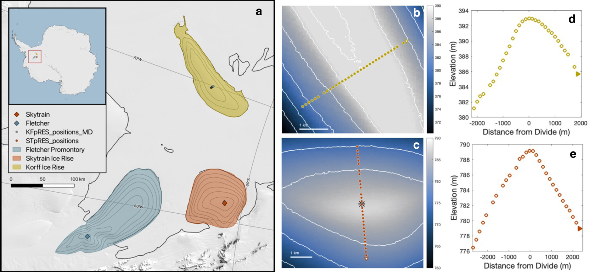
An ice divide runs the length of KIR, a slow-moving, 600-m-thick area of grounded ice surrounded by the Ronne Ice Shelf. Kingslake and others (Reference Kingslake, Martín, Arthern, Corr and King2016) suggest that the flow of KIR underwent a reorganization 1.9–2.9 ka ago, which is also evident in the ice fabric below the firn between 200 and 230 m (Brisbourne and others, Reference Brisbourne2019) and that it has remained approximately steady since this time. On 20–22 December 2013 and 5–7 December 2014, pRES was deployed at 35 locations (resulting in usable data from 33 locations), evenly spaced along a 4.4 km transect parallel to ice flow and perpendicular to the divide (Fig. 1b). A surface Global Navigation System Satellite (GNSS) survey measured horizontal surface velocities and showed that there is negligible flow parallel to the divide in this location (Kingslake and others, Reference Kingslake, Martín, Arthern, Corr and King2016). FP is a promontory-style ice rise (i.e. one which is connected to the main ice sheet by grounded ice; Matsuoka and others, Reference Matsuoka2015) with a triple-junction ice divide that generates a complex 3-D ice flow pattern (Hindmarsh and others, Reference Hindmarsh2011). In conjunction with a wider survey (Kingslake and others, Reference Kingslake2014), pRES measurements were taken at a single location (−77.900°, −82.614°) on 25 January 2014 and 13 January 2015, ~300 m from the site of an ice core (−77.902°, −82.605°; Mulvaney and others, Reference Mulvaney, Triest and Alemany2014). SIR, also a promontory-style ice rise, sits at the southwest edge of the Ronne Ice Shelf to the east of FP (Fig. 1). pRES was deployed at 31 points on 7–11 December 2013 and 8–11 January 2015 along a 5.2 km transect perpendicular to and crossing the divide, centered on the location of a full-depth ice core (−79.741°, −78.545°; Fig. 1c; personal communication from R. Mulvaney, 2021).
pRES is a stationary, step-frequency, ground-based radar system, which transmits and receives through two spatially separated antennas (Corr and others, Reference Corr, Jenkins, Nicholls and Doake2002). This system is the predecessor to the autonomous phase-sensitive radio-echo sounder (ApRES; Nicholls and others, Reference Nicholls2015). At each field site, the transmitting and receiving antennas were separated by 7 m and multiple measurements were made during each visit to each site while varying antenna orientations between measurements (for the full procedure see Kingslake and others, Reference Kingslake2014, Reference Kingslake, Martín, Arthern, Corr and King2016). For the measurements on KIR and SIR, the antennas were oriented along and perpendicular to the transect lines (Figs 1b, c; note that the polarimetric surveys on KIR reported by Brisbourne and others (Reference Brisbourne2019) were located ~50 km north of our transect). To obtain measurements of vertical velocity, we made repeat measurements at each site separated by ~1 year.
Table 1 summarizes ancillary data for each field site. We used the regional climate model RACMO2.3p2 (van Wessem and others, Reference van Wessem2018) to estimate mean accumulation rates at each site. We averaged mean annual accumulation rates between 1979 and 2015 and over 50 km radius, circular areas centered on the core sites on FP and SIR, and the center of the transect on KIR (Wearing and Kingslake, Reference Wearing and Kingslake2019). At the two locations where ice cores have been drilled, FP and SIR, we used measured multi-centennial-averaged (~1000 years) accumulation rates and the density of ice equal to the mean density of the core between a depth of 250 m and the bed (personal communication from R. Mulvaney, 2020). These densities are less than the commonly used 917 kg m−3 (Table 1). We use average annual surface temperatures estimated from a weather station on KIR (personal communication from R. Mulvaney, 2018) and from 10-m borehole temperatures measured at SIR and FP (Mulvaney and others, Reference Mulvaney, Triest and Alemany2014; Reference Mulvaney, Rix, Polfrey, Grieman, Martìn, Nehrbass-Ahles, Rowell, Tuckwell and Wolff2021). We assume that 10-m borehole temperatures represent the average annual air temperature.
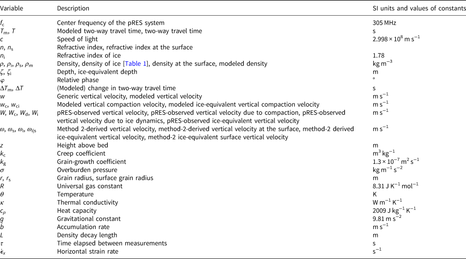
Climatic, ice core and pRES survey characteristics of the three field sites

RACMO-simulated accumulation rates (in meters ice-equivalent) are 40-year averages over a 50 km2 radius area centered on each field site. The measured accumulation rates and temperatures for FP and SIR are from Mulvaney and others (Reference Mulvaney, Triest and Alemany2014) and personal communication from R. Mulvaney (2021), where accumulation rates are recent, multi-centennial averages (~1000 years). Ice densities were measured in the field during drilling of ice cores on FP (Mulvaney and others, Reference Mulvaney, Triest and Alemany2014) and SIR (personal communication from R. Mulvaney, 2020). The KIR average temperature is from a British Antarctic Survey automatic weather station (AWS) that took measurements between 2014 and 2017 (personal communication from R. Mulvaney, 2018). The pRES-derived accumulation rates are estimated assuming a steady state (Section 2.4).
a Multi-centennial-averaged accumulation rates.
b Std dev. estimated by varying bounds on linear fit.
c 10-m borehole temperature.
d Range across the transect.
e AWS (1/2014–2/2017).
2.2. Phase-sensitive radio-echo sounder
pRES measures the response of the ice sheet to a range of frequencies over a bandwidth of 160 MHz centered on a frequency, f c = 305 MHz. At each frequency, the complex ratio between a transmitted and received signal is recorded. Following Corr and others (Reference Corr, Jenkins, Nicholls and Doake2002), an inverse Fourier transform of the frequency response yields power and phase as functions of two-way travel time, T.
To relate depth, ζ, to T, we use

where c is the speed of light in a vacuum (2.998 × 10⁸ m s−1) and the refractive index, n, depends on density through

where ρ i is the density of ice (see Table 1) and n i is the refractive index of ice (1.78) (see Kovacs and others (Reference Kovacs, Gow and Morey1995) for discussion of more complex and potentially more accurate relationships between ρ and n). At different stages throughout our methods, we define n using ρ as a function of ζ or T, as implied by the integral in Eqn (1).
Following Corr and others, Reference Corr, Jenkins, Nicholls and Doake2002, we assume that peaks in the pRES returns that persist between measurements move as material surfaces. We refer to these peaks as ‘reflectors’ even though they are generally assumed to be interference patterns resulting from many thinner layers, which are not explicitly resolved by the radar. Reflectors are chosen using an algorithm based on their brightness and phase coherence (for more details, see Corr and other, Reference Corr, Jenkins, Nicholls and Doake2002; Kingslake and others, Reference Kingslake2014). The distances between these reflectors change as firn compacts and the ice sheet flows. We track this by recording the relative phase (ϕ) of each reflector during two time-separated pRES measurements. For reflector j, we record $\phi _1^j$ and $\phi _2^j$
 in the first and second deployments, respectively. We difference these with the phase of a reference reflector identified in both years $\phi _1^{\rm R}$
 and $\phi _2^{\rm R}$
 to remove the effect of vertical displacement of the radar between measurements. The reference reflector is arbitrarily chosen as one that lies close to 100 m depth and can be unambiguously identified in returns from both time-separated deployments (Kingslake and others, Reference Kingslake2014).
If one assumes uniform density, these relative phase differences can be straight-forwardly expressed as a fraction of a wavelength and therefore a relative vertical displacement (e.g. Kingslake and others, Reference Kingslake2014). As we are concerned with strain in the firn where ρ varies vertically, we express changes in two-way travel time as a function of change in relative phase for each layer j:

The phase changes can be measured to an accuracy of up to ~1°, which translates into a ΔT on the order of nanoseconds. The uncertainty of each ΔT j is estimated following Kingslake and others (Reference Kingslake2014; their Section 2.1). A reflector phasor is generated from the strength and phase of reflector j. It is combined with a noise phasor with a magnitude equal to the mean of the noise floor of the radar return and an assumed perpendicular orientation compared to the reflector phasor (corresponding to the maximum possible phase offset). This gives a conservative estimate of the uncertainty in the phase at each reflector. To increase the signal-to-noise ratio, the ΔT j values are stacked into ~10-m (0.12 ms) bins by calculating the mean in each bin weighted by the inverse square of the measurement uncertainties (Kingslake and others, Reference Kingslake, Martín, Arthern, Corr and King2016). The result is a profile of the change in two-way travel time as a function of the two-way travel time, ΔT(T).
2.3. Two methods for extracting densification rates from pRES observations
Here, we outline two methods to extract compaction rates from pRES data. For each method the key challenge is converting the quantities measured by pRES – two-way travel time, T, and change in relative two-way travel time, ΔT – into depth and compaction velocity. Method 1 uses densities measured from coincident ice cores to make these conversions. Method 2 uses a mass-conserving inverse method to estimate depth, compaction velocity and density. It does not require density measurements but assumes a steady-state exponential density profile. Note that we use different symbols to differentiate various vertical velocities: W refers to velocities derived from pRES observations, ω refers to the vertical velocity minimized for in Method 2, and w both refers to the vertical velocity modeled by the physics-based compaction model (Section 2.5) and is used generically in equations that apply to more than one vertical velocity. All variables are shown in Table 2.
List of variables
2.3.1. Method 1: compaction velocities using independently measured densities
To translate T into ζ for any particular reflector, we need to know the density at and above that reflector. We transform the depth of an ice core into T using

and then use linear interpolation to estimate the ice-core-derived density at the T of each binned pRES measurement.
The vertical velocity, W, of each englacial reflector relative to a reference reflector is computed as follows:

where Δτ is the time between radar measurements. We then use Eqn (1) to compute ζ for each reflector in the pRES returns.
Following Jenkins and others (Reference Jenkins, Corr, Nicholls, Stewart and Doake2006) and Morris and others (Reference Morris2017), we assume the total vertical velocity can be separated into two components: an ice-dynamic component, W d, generated by horizontal divergence or convergence of the ice sheet, and a vertical firn compaction component, W c. If u represents horizontal velocity, mass conservation in the incompressible part of the ice column beneath the firn, $ {{\partial u}/{\partial x}} + {{\partial w}/{\partial z}} = 0 $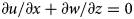 , allows us to estimate the horizontal strain rate, $\dot{\epsilon }_x = \partial u/\partial x$
 , from the pRES-measured vertical strain rate, $\dot{\epsilon }_z = \partial w/\partial z$
 , by assuming that all vertical velocities, and therefore all vertical strain rates, measured below the firn are due to horizontal convergence or divergence. Following Kingslake and others (Reference Kingslake2014), we assume contributions from v and $\dot{\epsilon }_y = \partial v/\partial y$
 are negligible along the flanks of ice rises. This approach is further simplified by assuming that the horizontal strain rate is constant in the top two-thirds of the ice column (above bed effects), and therefore W d is linear, which is consistent with the shallow ice approximation (SIA; Lliboutry, Reference Lliboutry1979; Wearing and Kingslake, Reference Wearing and Kingslake2019). These assumptions allow us to estimate W d using a linear least-squares fit to the pRES-measured W (Eqn (4)) in the middle third of the ice column, below the firn–ice transition and above bed effects, and then extrapolate this fit to the surface, giving W d in the ice and firn. At FP, we use 160 < ζ < 309 m as the depth range for the linear fit, at SIR we use 122 < ζ < 304 m and at KIR we use 150 < ζ < 300 m. The boundaries for FP and SIR were chosen by minimizing the mismatch between the core density and the density inverted for in Method 2 (Section 2.3.2), although the ice-core-measured densities could also be used to choose these bounds. We discuss the impact of the choice of upper and lower boundaries on the results in Section 4. Once W d is estimated, the compaction velocity, W c, can be isolated by subtracting W d from the observed radar velocity, W c = W − W d.
2.3.2. Method 2: inverting for density and vertical velocity
Method 2 addresses a common scenario where we have pRES observations without coincident density measurements. In this case, we must estimate $n(\rho)$ to obtain vertical velocities from Eqn (4). We estimate ρ by solving the compressible mass conservation equation for the vertical velocity, which depends on ρ, and minimizing the least-squares difference between this optimized velocity, ω, and pRES observations converted into velocities, which also depends on ρ. It is convenient to follow Kingslake and others (Reference Kingslake, Martín, Arthern, Corr and King2016) in defining the ice-equivalent velocity (units of meters ice equivalent, or m i.e.), which depends only on the pRES measurements and is independent of density, as:

We assume vertically uniform horizontal strain rates in the top two-thirds of the ice due to ice flow (as in Method 1) and that ∂ρ/∂x is negligible locally. Conservation of mass under these conditions gives

The density profile is approximated by an exponential function:

where ρ s is the surface density and L is the decay length.
Substituting Eqn (7) into Eqn (6) and integrating vertically yields:

where ω s is the vertical velocity at the surface. To relate ω to the pRES observations we apply the definition of ice-equivalent velocity (Eqn (5)) to define an ice-equivalent velocity ω i and a corresponding surface velocity ω i|s as


Substituting ω i and ω i|s into Eqn (8) and rearranging gives

Equation (10) shows that the total vertical velocity equals the vertical velocity at the surface plus the second term on the right, which represents the cumulative effect of horizontal strain (the first term in square brackets) and increasing density (the second term in square brackets) on vertical velocity. This term is zero at the surface and, because it is negative, acts to reduce the magnitude of ω i from its surface value by an amount that increases with depth and density (note that lowering L and increasing ρ s increases this term and the density). It increases with depth because the impact of the strain rate accumulates over the ice column. It increases with density because, due to mass conservation, the impact of a given horizontal strain rate on vertical velocity increases with ρ.
As in Method 1, we estimate $\dot{\epsilon }_x$ as the slope of a linear least-squares fit to ω i(ζ) so that Eqn (10) contains three unknown parameters: ρ s, ω i|s and L. Using MATLAB's fminsearch we minimize the square of the difference between the pRES-measured W i (Eqn (5)) and ω i (Eqn (10)) to estimate optimal values for the three unknowns:

where $\zeta_b$ is the lower bound of the region where the horizontal strain rate is considered constant. With these parameters, we compute the density profile using Eqn (7). Finally, the density profile is used to convert T and $\Delta T$
 into ζ and W using Eqns (1) and (4), respectively.
As in Method 1, the firn compaction velocity W c is extracted by subtracting the ice-dynamic contribution, W d, from W.
2.4. Estimating accumulation rates from pRES data
The average accumulation rate,$\;\dot{b}$ , is a useful environmental indicator, and serves as a boundary condition in the physics-based compaction model (Section 2.5). As an alternative to ice-core measurements or regional climate models, we can use pRES measurements to estimate $\dot{b}.$
 If we assume that ice-sheet thickness is in steady state at our field sites, $\dot{b}$
 equals the ice-equivalent vertical velocity at the surface: ignoring ablation, the accumulation must balance downward advection for the surface height to remain constant. To calculate the vertical velocity at the surface, we used a linear least-squares fit to the middle third of pRES-derived profiles to find W i(ζ) (see Section 2.3.1 for the depth ranges used), then extrapolated this linear fit to the surface to estimate the surface ice-equivalent vertical velocity. We compared these estimates to ice-core measurements and 40-year mean accumulation rates simulated using RACMO2.3p2 (Section 2.1, Table 1). As a boundary condition on the firn compaction model described in the next section, we used these pRES-derived accumulation rates at all KIR sites and all but one SIR site, and core-derived accumulation rates at FP and the SIR pRES site closest to the core (site 18).
2.5. Firn compaction model
2.5.1. Equations
Our model closely follows the model proposed by Arthern and others (Reference Arthern, Vaughan, Rankin, Mulvaney and Thomas2010) (their Appendix B), except that we take a Eulerian approach instead of a Lagrangian one. We define a 1-D Eulerian coordinate system where the vertical coordinate z is positive upward and the vertical velocity w is positive downward. We use ρ m to denote a ‘modeled density’ to distinguish it from other densities defined earlier. As all deformation in this model is due to firn compaction, w is related to density through mass conservation:

where D/Dt is the material derivative $\left({=}{{\partial}/{\partial t}} - w {\partial / {\partial z}}\right)$ . Integrating upward from the firn–ice transition, z t, gives

where w t is the velocity at the base of the firn pack that we impose (Section 2.5.2). Following Arthern and others (Reference Arthern, Vaughan, Rankin, Mulvaney and Thomas2010), we describe firn densification as a function of overburden pressure, σ, temperature, θ, grain radius, r and density, ρ m, as follows:

where R is the universal gas constant (8.31 J K−1 mol−1), E c is the activation energy for diffusion creep and is found by minimizing the mismatch between the modeled and observed velocities or densities (Section 2.6), and k c is a constant that depends on the density regime:

To track ρ m on the Eulerian grid, we expand the left side of Eqn (14) using the definition of the material derivative to give

Defining σ = 0 at the surface,

where g is the gravitational constant (9.81 m s−2). Temperature, θ, evolves as

where the heat capacity cp = 2009 J kg−1 K−1 (Paterson, Reference Paterson1994) and the thermal conductivity κ depends on the local density as κ(ρ m) = 2.1(ρ m/ρ i)2 W m−1 K−1 (Arthern and Wingham, Reference Arthern and Wingham1998). The square of the grain radius increases with time according to an Arrhenius temperature dependence and is advected with flow:

where E g is the activation energy for volume self-diffusion and is found by minimizing the mismatch between the modeled and observed velocities or densities (Section 2.6), and k g is the grain-growth coefficient, 1.3 × 10⁻⁷ m2 s−1 (Arthern and others, Reference Arthern, Vaughan, Rankin, Mulvaney and Thomas2010). Note that grain growth is independent of overburden pressure.
2.5.2. Boundary conditions
To conserve mass globally and allow a steady state to be reached, we impose a lower boundary condition w(z t) = $\dot{b}$ , where $\dot{b}$
 is the ice-equivalent accumulation rate found in Section 2.4 at all locations except those nearest to the FP and ST ice cores, where ice-core-measured rates are used instead (Table 1, personal communication from R. Mulvaney, 2021). For temperature boundary conditions (Eqn (18)) we used the mean annual surface temperatures listed in Table 1 at the model's upper boundary and at the model's lower boundary we used the temperature gradient measured at FP at the depth where ρ = 900 kg m−3, ${\partial \theta}/{\partial z}$
 = 0.0034 K m−1. Following Arthern and others (Reference Arthern, Vaughan, Rankin, Mulvaney and Thomas2010), we used a surface grain radius of r s2 = 10−9 m. As no field measurements of surface density were available, we estimated ρ s by extrapolating the density profiles at FP and SIR using a widely used logarithmic function of depth (Herron and Langway, Reference Herron and Langway1980; their Eqns (7 and 10)) in the upper tens of meters. At FP ρ s = 435 kg m−3 and at SIR ρ s = 400 kg m−3. This approach likely overestimates the true surface density, as very-near-surface densification processes are not represented by the model of Herron and Langway (Reference Herron and Langway1980). However, it provides a reasonable boundary condition in the absence of direct field observations. The temperature boundary conditions, $\dot{b}$
 , ρ s and r s2 were held constant throughout all simulations.
2.5.3. Thickness evolution, numerical implementation and initial conditions
We solved the model equations numerically on a Eulerian grid with an initial thickness h = 250 m. For each time step, the grid was allowed to thin or thicken according to ${\rm d}h/{\rm d}t = \dot{b}( \rho _{\rm i}/\rho _{\rm s}) \;-\;w_{\rm s},\;$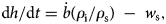 where w s is the velocity at the surface, and the gridpoints were repositioned (ensuring a grid spacing of ~0.33 m); all variables were interpolated onto the new grid. We used a time step of 0.001 years (~9 h). Density was initialized with an exponential profile (Eqn (7)) with L = 40 m (note that in Method 2 above L was treated as an unknown). The initial temperature profile linearly increased with depth at a rate of 0.0034 K m−1 (the gradient measured in the FP borehole). Velocity was calculated every time step using Eqn (13) and the values of σ, ρ m, θ and r 2 from the previous time step. Density, grain size and temperature were updated from the previous time step using Eqns (16–19). Simulations terminated when ${\partial \rho_m}/{\partial t}$
 < 10−6 kg m−3 s−1, approximating a steady state.
2.6 Using densification rates to tune models
A common procedure in firn modeling is to tune model parameters to observations of density (e.g. Herron and Langway, Reference Herron and Langway1980) or compaction (Arthern and others, Reference Arthern, Vaughan, Rankin, Mulvaney and Thomas2010; Morris, Reference Morris2018). We investigate how the optimal values of the grain growth and compaction activation energies, E g and E c, of the model (Section 2.5), depend on whether we optimize using compaction velocities (estimated with pRES) or density profiles (measured in the two ice cores). All optimization was performed in MATLAB using fminsearch to minimize the least-squares difference between modeled and measured densities and compaction velocities, where modeled values were first interpolated to the depths of pRES measurements or density measurements for comparison.
2.7. Comparing models with pRES observations
Finally, we introduce a method for comparing model output to radar observations. This approach converts modeled depth and compaction velocities into two-way travel time, T m (to denote ‘modeled two-way travel time’) and relative change in two-way travel time, ΔT m, so that they can be directly compared to the respective pRES measurements. Here, we use the model presented in Section 2.5, although any compaction model could be used. As a reminder, W denotes pRES-derived velocities (Eqn (4)) and w c denotes modeled compaction velocities (Section 2.5). Compaction velocities are modeled as described in Section 2.5, where activation energies are tuned to the pRES measurements at FP, and to sites 18 and 5 for the transects across SIR and KIR, respectively. Modeled compaction velocity, w c, is converted into an ice-equivalent velocity w ci using Eqn (5). We then add the component of vertical velocity due to the horizontal strain rate, W d (estimated using a linear fit to the pRES-derived ice-equivalent velocity, W i) to w ci to estimate a modeled, ice-equivalent, total vertical velocity, w i = w ci + W d. Then w i and the depth of each modeled gridpoint is converted into ΔT m and T m, respectively, using the modeled density profile (ρ m), as follows:


These modeled values can then be directly compared to quantities observed by pRES, ΔT and T.
3. Results
3.1 Compaction velocities and density profiles
At all sites, compaction velocities are fastest at the surface (or as close to the surface as possible, given the constraints of the pRES system) and decrease with depth until they approach zero at the bottom of the firn–ice transition zone.
Figures 2a, c show compaction velocities from FP estimated from pRES measurements using Method 1 (Section 2.3.1) and densities measured in the FP core. The pRES-estimated compaction velocity is 0.22 m a−1 at 12 m depth, just below the first density transition zone of 550 kg m−3. The firn reaches the pore close-off density (830 kg m−3) at 79 m (Mulvaney and others, Reference Mulvaney, Triest and Alemany2014); compaction can be seen until ~130 m, below which velocities approach zero, with fluctuations of 0.01 m a−1 or less.
Core observations, modeled velocity and densities, and Method 1 compaction velocities. Left panels are from FP, the right panels are from SIR, top panels are compaction velocities and bottom panels are densities. In the top panels (a, b), blue squares are compaction velocities derived from pRES measurements using Method 1. Uncertainties are derived by taking into account the signal-to-noise ratio of each englacial reflector used to computed vertical velocities (Section 2.2) and are represented by the width of the bar symbols. Gray circles in the bottom panels are ice core-measured densities. The dashed and dotted curves show the model output (Section 2.5), where the dashed blue lines are generated from a model tuned to pRES vertical velocities, and the dotted black lines are generated from a model tuned to core densities. The gray horizontal dashed and dot-dashed lines show where core-derived densities are 550 and 830 kg m−3, respectively, corresponding to the compaction transition density identified by Herron and Langway (Reference Herron and Langway1980) and the lock-in density.
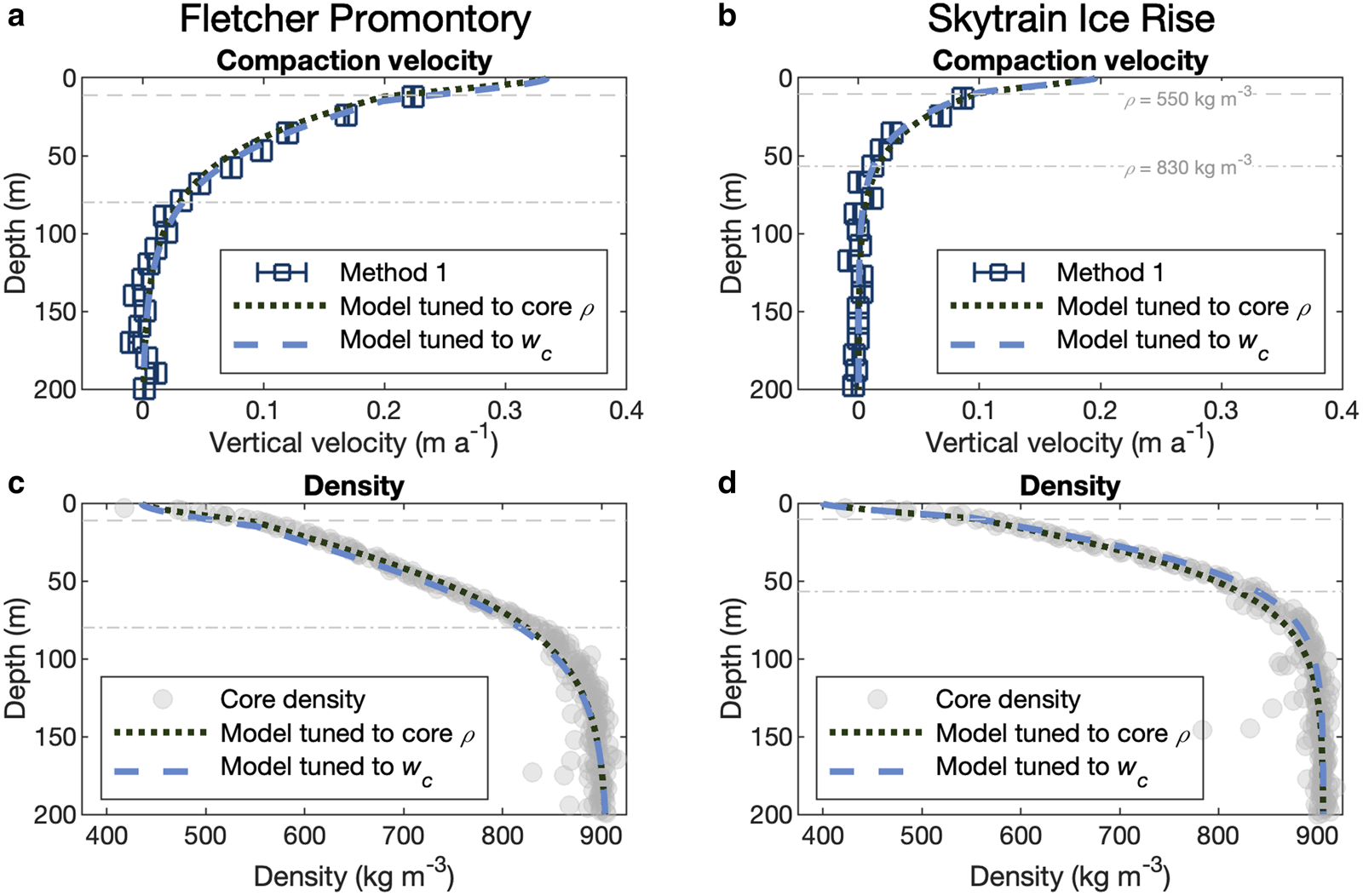
Figures 2b, d show Method 1 compaction velocities from site 18 on SIR (the pRES measurement closest to the SIR core), and densities measured from the SIR core. Compaction velocities are slower than that at FP, likely due to lower accumulation rates (Table 1). The pRES-estimated compaction velocity is 0.09 m a−1 at 13 m depth, just below the first density transition zone of 550 kg m−3. The firn reaches the pore close-off density at 56 m (personal communication from R. Mulvaney, 2021); compaction can be seen until ~85 m. Like at FP, below this depth velocities approach zero, with fluctuations of 0.01 m a−1 or less.
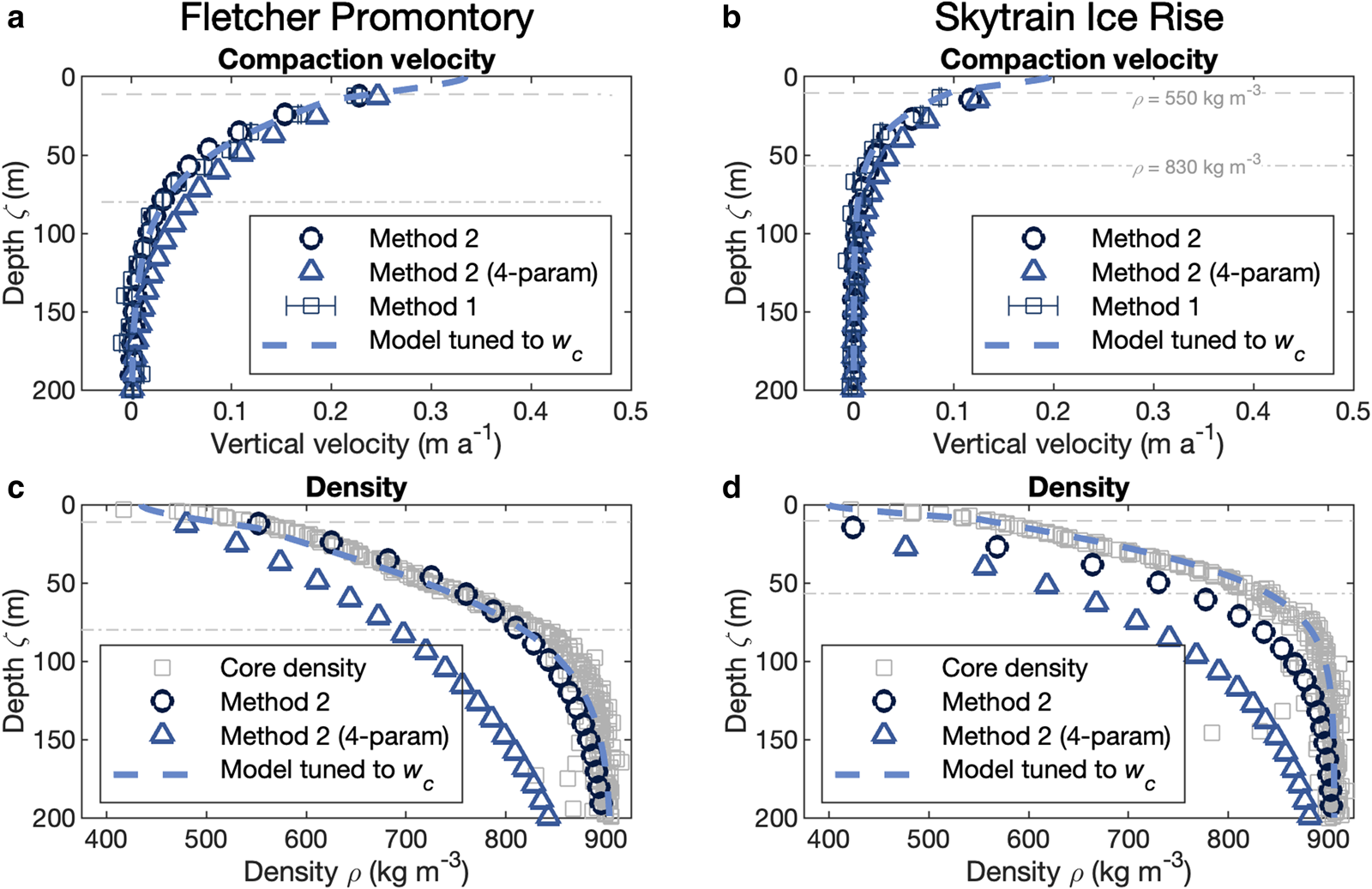
Method 2 employs a simple inversion to simultaneously estimate vertical profiles of density and compaction velocity. It is useful for locations without independent density measurements. We apply it to the ice-core adjacent pRES measurements at FP and site 18 on SIR to assess the methodology (Fig. 3), and then across the KIR and SIR transects, which have no density measurements (Fig. 4).
Inverted compaction velocities and densities from Method 2 at FP and SIR. Method 2 inverts for a density profile and velocity given pRES measurements of the ice-equivalent vertical velocity. In (a) and (b), Method 2 compaction velocities in blue circles are compared to compaction velocities from Method 1 (blue squares) and the model (blue dashed line; Section 2.5) at FP and SIR. At FP, Method 2, the model and Method 1 agree at all depths within 0.02 m a−1. The four-parameter inversion (triangles), described in the discussion, overestimates the firn compaction velocity between ζ = 25 m and the firn–ice transition. At SIR, Method 2 agrees with Method 1 velocities to within 0.01 m a−1 below ζ = 20 m, while the four-parameter inversion overestimates the compaction velocity by 0.02–0.03 m a−1. In (c) and (d), densities of Method 2 are compared to core observations (gray squares) and the pRES-tuned model densities (dashed blue lines). At FP, Method 2 agrees with the density profile until 800 kg m−3 below which it underestimates the density. The four-parameter inversion underestimates the density by 50–150 kg m−3. At SIR, Method 2 and four-parameter inversions underestimate density by 50–100 and 100–200 kg m−3, respectively. The gray horizontal dashed and dot-dashed lines show where core-derived densities are 550 and 830 kg m−3, respectively.
Spatial variability of total velocities and compaction velocities at SIR and KIR obtained using Method 2. Method 2 can generate compaction velocity profiles at locations where we lack coincident density profiles across two transects, a northeastern–southwestern transect on KIR (black-to-blue gradient, Fig. 1b) and a north-to-south transect on SIR (black-to-blue gradient, Fig. 1c). Panels a and b show the total vertical velocity measured by each of the pRES points along KIR and SIR, respectively. Panels c and d show the firn compaction velocity. Note in panel a at KIR, the eastern flank (light blue) generally flows faster than the western flank, but that this trend is not evident in the compaction velocity estimates (c). The triangle to the right of the colorbar indicates the orientation of the transects in Figures 1b, c.

Figure 3 compares the results of Method 2 (Section 2.3.2) to the results of Method 1 (Section 2.3.1) and the pRES-tuned model (Section 2.5). Figure 3a shows that at FP, compaction velocities from Method 2, Method 1 and the model agree to within 0.02 m a−1. Figure 3c shows that the density estimated with Method 2 largely agrees with the observed density, until ~800 kg m−3, reaching ice density 20–30 m deeper than the core densities, while staying within 25 kg m−3 of the observations.
In Fig. 3b, Method 2 compaction velocities at SIR site 18 match those computed with Method 1 to within 0.025 m a−1 in the region above 20 m depth and within 0.01 m a−1 in the region below. Method 2 compaction velocities decay to zero near 100 m depth, ~20 m below the Method 1 firn–ice transition. Figure 3d shows that Method 2 results in densities 100–200 kg m−3 lower than the observed densities. This is due, in large part, to an underestimation of the surface density and overestimation of L by the minimization.
Figure 4 shows results from applying Method 2 to locations on SIR and KIR. Across KIR in Figure 4a, we see a gradient in total vertical velocities across the divide. After removing the ice dynamic component to obtain firn compaction velocities, this gradient is largely absent (Fig. 4c). Within 25 m of the surface, firn compaction velocities across KIR vary between 0.05 and 0.17 m a−1. Despite this variation in near-surface firn velocities, at most locations, the firn–ice transition zone is reached near the same depth, ~150 m, although a few sites show small (<0.01 m a−1) compaction velocities below this depth.
At SIR (Figs 4b, d), we do not see a gradient across the transect in either total velocities or compaction velocities. Between the surface and 25 m depth, compaction velocities range from 0.05 to 0.14 m a−1. At most sites the compaction velocities reach zero above 150 m; however, as at KIR, data at a few sites show compaction much deeper.
3.2 Estimated accumulation rates
Figure 5a shows that at SIR, pRES-derived accumulation rates are 0.09–0.11 m i.e. a−1 near the divide and are systematically larger on the flanks (>500 m from the divide; Figs 1c, e), with the largest accumulation rates of 0.14–0.16 m i.e. a−1 at the northern end of the transect. In comparison, multi-centennial-averaged accumulation rates measured from the SIR ice core are 0.15 ± 0.02 m i.e. a−1 (personal communication from R. Mulvaney, 2021). RACMO accumulation rates in the area are slightly higher, at 0.23 ± 0.05 m i.e. a−1 (Section 2.1; Table 1).
pRES-derived accumulation rates at SIR and KIR. Accumulation rates (blue triangles) are derived using the steady-state assumption described in Section 2.4. Solid lines show the average accumulation rate of each flank using points >500 m from the divide. The average accumulation rates at SIR (a) are the same on both flanks, while at KIR (b), the northeast flank (right side of plot) has on average 0.04 m i.e. a−1 higher accumulation than the southwest flank (left side of plot). The filled triangles orient the transects with respect to Figure 1. The light blue circles show the elevation change and topography of the transect as interpolated from REMA.

At KIR, pRES-derived accumulation rates are larger on the northeast side of the divide than on the southwest side. In Figure 5b, on the southwest side, 1000 m or more from the ice divide (Figs 1b, d), pRES-derived accumulation rates are 0.13–0.18 m i.e. a−1. On the northeast side, accumulation rates are 0.20–0.22 m i.e. a−1. These values are in broad agreement with accumulation rates from RACMO, 0.21 ± 0.03 m i.e. a−1.
At FP (not shown in Fig. 5), the pRES-derived accumulation rate is 0.40 m i.e. a−1, which exceeds the revised 0.30 m i.e. a−1 multi-centennial-averaged rate measured by Mulvaney and others (personal communication from R. Mulvaney, 2021). Both accumulation estimates are in agreement with accumulation rates from RACMO, 0.38 ± 0.08 m i.e. a−1.
3.3 Modeled firn compaction velocities
In Figures 2 and 3, Methods 1 and 2 are compared to steady-state compaction velocities modeled with the physics-based model (Section 2.5). Figure 2 plots two model outputs with different activation energies, tuned to minimize the least-squares difference between the model and either the ice-core density measurements or the pRES-derived densification rates. Figure 3 shows model results from the latter.
Figures 2a, b show that the model reproduces the Method-1-derived vertical compaction rates at both FP and SIR. The best-fit activation energies when tuned to the pRES observations at FP are E c = 68.7 kJ and E g = 50.3 kJ and at SIR are E c = 66.8 kJ and E g = 49.2 kJ. The best-fit activation energies when tuned to the ice-core densities from FP are E c = 67.1 kJ and E g = 48.6 kJ and from SIR are E c = 66.5 kJ and E g = 48.5 kJ. The pRES-tuned model reproduces Method 1 compaction velocities at both sites. The density-tuned model tends to underestimate Method 1 velocities by <0.03 m a−1 at FP, and agree with Method 1 at SIR.
Figures 2c, d show that at FP and SIR we find close agreement between modeled and measured densities, especially above the lock-in depth (ρ = 830–850 kg m−3). At FP, the pRES-tuned model predicts slightly lower densities than measured (by <30 kg m−3) at depths between the surface and 45 m (ρ < 700 kg m−3). Between 45 m and the lock-in depth (where ρ = 830 kg m−3), both models agree within 10 kg m−3 to each other and the core; below the lock-in depth, the models show lower densities, achieving ice density 20 m below the ice core.
At SIR, both the pRES- and core-tuned models agree with the measured densities within <5 kg m−3 between the surface and 15 m. Below 15 m, the pRES-tuned model overestimates the density by <20 kg m−3 until the firn–ice transition, and reaches ice density at about the same depth as the ice core. The core-tuned model gives slightly lower densities than observations below the lock-in depth, and reaches the firn–ice transition ~15 m below the observations.
3.4 Modeled pRES observations
Finally, the method described in Section 2.7 compares two-way travel times and change in two-way travel times derived from the physics-based model to pRES measurements. Figure 6 shows that two-way travel times are on the order of microseconds (panels a, c, e), changes in two-way travel time are on the order of nanoseconds (panels a, c, e), and the model results agree with pRES observations to within 5–20%.
Modeled (solid lines) and measured (circles) two-way travel time, T, and change in two-way travel times, ΔT, at FP (a, b), SIR (c, d) and KIR (e, f). The left column shows ΔT as it changes with T on FP (a) and at four randomly selected locations (differentiated by color) along SIR (c) and KIR (e). The model was run with activation energies obtained by optimizing the model output to the results of Method 1. The right column shows the normalized mismatch in ΔT, (ΔT − ΔT m)/ΔT), as a percentage. The colors correspond to the randomly selected locations shown in the left panels, and the gray boxes show the normalized mismatch at all other locations along the transects of KIR and SIR. ΔT andΔT m agree at all locations and depths to within 20%. At FP, the model overestimates ΔT in the top 30 m. Note the variable horizontal axes in the left panels.

For FP, Figs 6a, b show that the modeled two-way travel times are within 10% of the measured values throughout the profile except for T m < 0.5 ms, where the change in two-way travel time is overestimated by the model.
At SIR, Figs 6c, d show that the model largely agrees with the observations, with a tendency to underestimate the change in two-way travel time in the near surface; the model mostly reproduces ΔT within 15% of pRES observations.
At KIR, Figs 6e, f show that the model slightly underestimates the change in two-way travel time; the model reproduces ΔT within 15% of pRES observations at most sites, and within 20% at the rest. Although not depicted in Fig. 6, both the model and the pRES observations indicate an accumulation gradient across the divide, where the southwest flank, with lower accumulation rates, has smaller changes in two-way travel time, and the northeast flank, with higher accumulation rates, has larger changes in two-way travel time.
4. Discussion
We have shown that we can measure firn densification with a ground-based phase-sensitive radar. We have presented two methods to isolate firn compaction velocities from pRES observations of vertical velocity using simple assumptions about horizontal ice flow and/or density. Method 1 uses an independently measured density to convert the relative change in two-way travel time into a profile of vertical velocity, then isolates the firn compaction component by removing the contribution of horizontal strain rate due to ice flow from the total velocity (Section 2.3.1). The compaction velocities extracted using this method closely match velocities simulated by a modified version of the physics-based compaction model described by Arthern and others (Reference Arthern, Vaughan, Rankin, Mulvaney and Thomas2010). Method 2 extracts firn compaction velocities in cases where we lack coincident density measurements. Using conservation of mass and an exponential expression to describe density, this simple inverse method produced compaction rates that broadly agree with the results of Method 1 and modeled compaction rates, even in the presence of the erroneous vertical variations in pRES-derived velocities seen at some SIR locations (these are discussed more below).
We also detail a method for extracting accumulation rates from the pRES observations at locations where a steady state can be assumed. We compare these to rates measured in ice cores and modeled using RACMO2.3p2. Modeled accumulation rates agree within uncertainty bounds to pRES-derived rates, except at SIR where the model estimate exceeded both the pRES-derived values and the ice core-measured values. At KIR this agreement and the steady-state assumption were consistent with the results of Kingslake and others (Reference Kingslake, Martín, Arthern, Corr and King2016), which indicated steady ice thickness on the centennial to millennial timescale. The spatial variability exhibited by the pRES-derived accumulation estimates need to be verified against independent high-resolution accumulation estimates (e.g. from shallow radar profiling or shallow cores); however, our results indicate that accumulation may increase southwest to northeast across the ice divide on KIR, which is consistent with the asymmetry in KIR's deep isochrones noted by Kingslake and others (Reference Kingslake, Martín, Arthern, Corr and King2016).
Using pRES to measure firn compaction has some advantages over previous methods. pRES is a lightweight, surface-based system that can be deployed by a single person, allowing many more point measurements to be made in a single field campaign than with, for example, borehole instrumentation. Moreover, pRES can measure vertical velocities from the near surface through to near the glacier bed, whereas firn-compaction measurements from borehole instrumentation (Arthern and others, Reference Arthern, Vaughan, Rankin, Mulvaney and Thomas2010) and airborne radar (Medley and others, Reference Medley2015) have been restricted to the upper tens of meters by instrument design and radio-wave penetration, respectively. Measuring full-depth velocity profiles is useful because it allows us to estimate and remove the contribution of horizontal strain rates in the firn. Some previous research has ignored this component of strain in the firn pack (Arthern and others, Reference Arthern, Vaughan, Rankin, Mulvaney and Thomas2010), while others have accounted for it using surface velocity fields (e.g. Morris and others, Reference Morris2017). An advantage of our approach is that we estimate the contribution of horizontal strain rates locally, and so it can be applied in slow-moving locations such as ice rises where ice cores are often drilled, but satellite-based surface velocities are unreliable. Removing the contribution of horizontal strain rate is perhaps more important in our study than in previous research because pRES measures compaction rates in the lower part of the firn pack, where the horizontal strain rates make up a higher proportion of the total strain than in the upper tens of meters. Finally, another advantage of our approach is that it can easily be applied to data collected using the successor to pRES, autonomous pRES (ApRES, Nicholls and others, Reference Nicholls2015). Due to its robust design and low power requirements, ApRES can operate autonomously for long periods, collecting near-continuous strain rate measurements. Future research using our methods could deploy ApRES to monitor seasonal or interannual variability in firn compaction.
Limitations of our methods are associated with which stresses contribute to compaction, the vertical variation of horizontal strain rates and density (particularly through their impact on the optimal parameters found in Method 2), a lack of near-surface radar returns, and the model we compare to our results. We discuss these in order below.
Following previous work (e.g., Jenkins and others, Reference Jenkins, Corr, Nicholls, Stewart and Doake2006), we assume that only hydrostatic stresses contribute to firn compaction in both the firn model and pRES-derived vertical strain rates. In the model, this leads to a simplified firn constitutive equation, Eqn (14). In the pRES data analysis, this assumption allows us to isolate strain rates associated with firn compaction from those associated with horizontal ice flow by assuming they are additive and separable. This approach is consistent Jenkins and others (Reference Jenkins, Corr, Nicholls, Stewart and Doake2006), who showed that at least in simple flow regimes, firn densification and ice-dynamic contributions to vertical velocity are independent. In more complicated flow regimes this may not be valid. For example, in shear margins, strain softening has been hypothesized to enhance firn compaction, thinning the firn pack enough to influence subglacial hydrology (Alley and Bentley, Reference Alley and Bentley1988; Riverman and others, Reference Riverman2019). Future research could take into account all stresses that potentially contribute to firn compaction by using a compressible, full-Stokes flow model (e.g. Licciulli and others, Reference Licciulli2020) and including a compressible, full-Stokes stress balance in minimization of Method 2, i.e. requiring that the derived firn compaction rates obey this stress balance as well as mass conservation.
A different, related issue is estimating horizontal strain rates. This is a significant source of uncertainty in our estimates of firn compaction rates and is relevant to all of our methods for analyzing pRES data. The SIA (Lliboutry, Reference Lliboutry1979) predicts approximately vertically uniform horizontal strain rates above the bed and has been applied to cold-based ice rise flanks before (Martín and others, Reference Martín and Gudmundsson2012; Kingslake and others, Reference Kingslake2014; Wearing and Kingslake, Reference Wearing and Kingslake2019). This motivates our decision to estimate the horizontal strain rate from the slope of a linear fit to pRES-measured vertical velocity profiles in the middle third of the ice column. However, pRES-measured vertical velocities deviate from linear in this region due either to erroneous vertical variability (i.e. noise; Kingslake and others, Reference Kingslake2014) in the data, or true variability not accounted for by the SIA, so the choice of upper and lower bounds on the linear fit introduces some uncertainty. For example, varying the upper and lower bounds by ±25 m changes our estimates of the vertical strain rate by up to 14% at FP, and by a similar amount elsewhere. This uncertainty propagates into all three of our methods. In Method 1, we removed the contribution of the horizontal strain rates to isolate firn compaction (Section 2.3.1); in Section 2.7, we added this contribution to our modeled firn compaction velocities to compare model outputs with radar observations. Estimates of firn compaction and density produced by Method 2 are affected in a particularly complex way by this uncertainty because we use $\dot{\epsilon }_x$ as an input to the minimization, which in turn impacts the optimal values for the surface density, density decay length and surface velocity. For example, at FP, a 14% change in $\dot{\epsilon }_x$
 leads to a 16% change in the density at 30 m but less than a 1% change in velocity at the same depth. This is largely driven by the inverted velocity's insensitivity to the decay length, L – a 14% change in $\dot{\epsilon }_x$
 can lead to up to a 65% change in L, which in turn affects the resulting density profile (Eqn (7)).
We explored a variety of alternative approaches to address uncertainty associated with estimating $\dot{\epsilon }_x$ . For example, instead of the three-parameter minimization of Method 2 (Section 2.3.2), we can consider $\dot{\epsilon }_x$
 unknown and optimize Eqn (11) for four parameters instead of three. This four-parameter inversion produces a good fit for ice-equivalent velocity (ω i); however, its insensitivity to L causes a large mismatch to the measured density, which translates into a worse match to the velocity W estimated with Method 1 (Eqn (4)), and thus the compaction velocity W c (Fig. 3). This is because computing $\dot{\epsilon }_x$
 from a linear fit to a region below the firn and prescribing this value in Method 2 is equivalent to performing the four-parameter inversion while, in effect, restricting the depth range used for the estimation of $\dot{\epsilon }_x$
 . In other words we more closely match pRES observations when we prevent the inversion from erroneously using velocity observations from shallower or deeper depths in its estimation of $\dot \epsilon_x$
 , where $\dot{\epsilon }_z$
 is not uniform. Another alternative is estimating horizontal strain rates from repeat GNSS surveys of poles installed in the ice surface. Kingslake and others (Reference Kingslake, Martín, Arthern, Corr and King2016) conducted such a survey on KIR. We find that applying Method 2 to the KIR data using either the point-by-point GNSS-derived horizontal strain rates or a spatially averaged value leads to velocities and densities with higher mismatches to pRES observations and core measurements than either the four-parameter minimization, described above or Method 2. Given these considerations, we suggest that estimating $\dot{\epsilon }_x$
 with a linear fit and employing Method 2 while optimizing for the remaining three parameters (as described in Section 2.3.2) is a reasonable choice, despite the uncertainty associated with selecting the vertical bounds on the linear fit. This simple approach also has the advantage that it can be applied to pRES data collected in locations without surface velocity measurements.
Firn density is required to translate pRES-observed two-way travel time (T) into depth, and the change in two-way travel time (ΔT) into velocities. Where independent density measurements are absent, we can invert for density using Method 2. When applied to pRES data collected near ice-core sites on FP and SIR, Method 2 produces vertical compaction rates that broadly agree with modeled compaction rates and with the results of Method 1 (which uses the ice core-derived density profiles). It also produces densities that broadly agree with ice core-measured densities at FP. However, because of our choice of a simple exponential function to describe the vertical variation of density, Method 2 consistently underestimates the density of deeper firn. Moreover, in some cases the minimization entirely fails to retrieve accurate density profiles when pRES measurements deviate significantly from the smooth vertical variation in ΔT expected from viscous ice flow and viscous-like compaction. In general, this impacts the estimate of the horizontal strain rate, which propagates through the inversion. For example, at SIR, Method 2 yields unrealistically high values of L and a poor fit to ice core-measured densities. Future research could address this limitation using a more complex description of the vertical variation of density, incorporating other geophysical surface measurements to add constraints on density, or imposing surface densities measured in the field (Fausto and others, Reference Fausto2018) or estimated with a climate model (Alexander and others, Reference Alexander, Tedesco, Koenig and Fettweis2019).
A final limitation of pRES (and its successor, ApRES) is that it was not designed to measure strain rates at depths shallower than ~10–15 m, which is where all or a majority of the first stage of densification (ρ < 550 kg m−3) occurs. The depth range covered by pRES can potentially complement shallower strain-rate measurements made in boreholes. The advantages to measuring deep strain rates include allowing the removal of horizontal strain rates from firn compaction estimates. However, future attempts to obtain better radar-based constraints on the early stages of densification could involve redesigning the radar system to specifically target shallower firn.
We compared our results to the densification model from Arthern and others (Reference Arthern, Vaughan, Rankin, Mulvaney and Thomas2010) because it integrates most of the known firn-compaction physics (e.g. grain sintering and growth, compaction due to overburden stress and heat flow). However, previous research has shown that this model displays some characteristics seemingly at odds with observations; for example, steady-state densities are only weakly dependent on accumulation rate (Lundin and others, Reference Lundin2017). Nonetheless, we compared the firn model to our observations of density and firn compaction and found close agreement between model results and the pRES observations after tuning model activation energies to the observations, giving us some confidence that the signal we have extracted from the pRES measurements accurately reflects firn compaction velocities.
Where pRES measurements of firn compaction and ice core-derived densities coincide, we have the choice of tuning activation energies to the compaction measurements or to the densities. Most firn densification models currently tune activation energies to firn cores. At SIR and FP, the activation energies tuned to either density or compaction agree to within 1 kJ, which indicates that both pRES and ice cores can be used to tune models of firn compaction. The activation energies we find to be optimal (Section 3.3) are larger than those used by Arthern and others (Reference Arthern, Vaughan, Rankin, Mulvaney and Thomas2010). The magnitudes of E c fall within the range of low-temperature (<−10°C) activation energies for volume self-diffusion estimated from in situ observations or laboratory experiments on ice (Weertman, Reference Weertman1983, their Table 3), although exceed the average value (59 kJ mol−1). The magnitudes of E g exceed the commonly used value for grain-boundary diffusion inferred from polar firn (42.4 kJ mol−1; Cuffey and Paterson, Reference Cuffey and Paterson2010)) and measured in laboratory experiments (40.6 kJ mol−1; Cuffey and Paterson, Reference Cuffey and Paterson2010). This mismatch may indicate other grain processes at work, or sensitivities that are not included in this model. Although activation energies encapsulate the sensitivity of a process to temperature, they themselves may be temperature-dependent (Li and Zwally, Reference Li and Zwally2004) and affected by the presence of impurities (e.g. Freitag and others Reference Freitag, Kipfstuhl, Laepple and Wilhelms2013). We ignored these effects and future research under controlled laboratory circumstances may be needed to disentangle them.
As in the low-density regime of the widely used Herron and Langway (Reference Herron and Langway1980) firn model, the steady-state density predicted by the model proposed by Arthern and others (Reference Arthern, Vaughan, Rankin, Mulvaney and Thomas2010) is largely independent of the accumulation rate (Lundin and others, Reference Lundin2017). This is a result of a tradeoff: in a steady-state, high accumulation rates bury low-density, small-grained snow faster, tending to lower the density at a given depth through advection (second term on the right side of Eqn (15)). However, because compaction rates are inversely proportional to grain size, this small-grained snow compacts faster (Eqn (15)). In this model, these processes compensate for each other, reducing the sensitivity of steady-state densities to accumulation. Ligtenberg and others (Reference Ligtenberg, Kuipers and van den Broeke2014) addressed an apparent discrepancy between this model behavior and observations by adding an accumulation-dependent factor, but accumulation dependence remains a source of disagreement among models (Lundin and others, Reference Lundin2017). In future research, widespread, long-term (multi-year) phase-sensitive radar measurements may help untangle the relationship between temperature, accumulation, density and densification rate by taking measurements at locations with similar average temperatures but varying accumulation rates, and vice versa.
5. Conclusions
The pRES and its update, the ApRES, have been deployed widely across Antarctica, Greenland and elsewhere to measure basal melt rates (Corr and others, Reference Corr, Jenkins, Nicholls and Doake2002; Jenkins and others, Reference Jenkins, Corr, Nicholls, Stewart and Doake2006; Nicholls and others, Reference Nicholls2015), ice fabric (Jordan and others, Reference Jordan, Schroeder, Elsworth and Siegfried2020; Young and others, Reference Young2020), englacial velocities (Kingslake and others, Reference Kingslake2014, Reference Kingslake, Martín, Arthern, Corr and King2016) and glacial hydrology (Vaňková and others, Reference Vaňková2018). As our study demonstrates, these systems also record firn densification.
We presented two methods for extracting firn compaction information from phase-sensitive radar data, and an additional method for comparing compaction models to pRES observations. Despite uncertainty about the contribution of ice flow to vertical velocity and limited observations in the upper 10–15 m, these methods generate compaction rates in close agreement with the steady-state output of a physics-based firn model. This gives us some confidence that the signal we are extracting from the pRES measurements is an accurate representation of firn compaction. However, we require coincident pRES (or ApRES) and independent firn compaction measurements (perhaps from down-borehole instrumentation) to fully validate this approach.
We highlighted three surveys in the Weddell Sea sector. Other, more spatially widespread and/or temporally near-continuous pRES/ApRES measurements performed primarily for other purposes may contain valuable information about firn compaction. In particular, pRES/ApRES measurements that coincide with density profiles could help constrain firn models, and ultimately improve estimates of mass balance from altimetry and climate reconstructions from ice cores.
Of particular interest to the firn modeling community is the temporal and spatial variability of densification and the dependence of firn density on the accumulation rate (Lundin and others, Reference Lundin2017). For example, Arthern and others (Reference Arthern, Vaughan, Rankin, Mulvaney and Thomas2010) took continuous measurements of compaction velocities, which varied by an order of magnitude between sites and by a factor of five at the same site over a few years. Others have modeled the influence of seasonal temperature variation on compaction (Zwally and Li, Reference Zwally and Li2002; Li and Zwally, Reference Li and Zwally2004; Li and others, Reference Li, Zwally and Comiso2007) and observed impurity-related (Hörhold and others, Reference Hörhold2012; Freitag and others, Reference Freitag, Kipfstuhl, Laepple and Wilhelms2013) changes in compaction. Phase-sensitive radars offer the community an opportunity for long-term, near-continuous measurements of compaction rates, which can be leveraged to clarify the impact of temperature and accumulation rate changes on firn compaction.
Acknowledgements
The authors thank R. Mulvaney, British Antarctic Survey (BAS), for supplying ice density data, and Rob Arthern, Carlos Martin, Hugh Corr and Richard Hindmarsh, for assistance with field survey design and operation of the pRES system, mentoring of JK, and discussion of the firn model and inverse methods. pRES and GNSS data are available from the UK Polar Data Center (http://doi.org/99b and http://doi.org/99c). The fieldwork was funded by Natural Environmental Research Council grant NE/J008087/1, led by Richard Hindmarsh, BAS. Logistical support was provided by many members of the British Antarctic Survey's air unit and field operations team. The authors thank particularly Iain Rudkin and Scott Webster for their assistance in the field, Melchior van Wessem for providing the RACMO2.3p2 data, and Ian Hewitt, Tun Jan (TJ) Young and an anonymous reviewer for their excellent feedback, which greatly improved this publication. We acknowledge the Norwegian Polar Institute's Quantarctica package for use in creating Fig. 1. We also acknowledge funding from National Science Foundation grants 1738934 and 1935438. This paper is based upon work supported by the National Science Foundation Graduate Research Fellowship Program under Grant No. (1644869). Any opinions, findings and conclusions or recommendations expressed in this paper are those of the author(s) and do not necessarily reflect the views of the National Science Foundation. The associated code and data are available for download at https://github.com/elizabethcase/pRES-firn-compaction-methods (doi: 10.5281/zenodo.5090283).


 Open access