

1. Introduction
Melting or freezing at the bottom of Antarctic ice shelves can make a significant contribution to their mass balance and hence to the mass balance of the Antarctic ice sheet. Bottom fluxes can be found from studies of the mass transfer through sections of an ice shelf provided that assumptions can be made about possible non-equilibrium behaviour. Alternatively, by assuming a value for the steady-state bottom flux supported perhaps by oceanographic measurements, estimates can be made of the rate of thickening of an ice shelf and the rate of advance of its grounding line (Reference ThomasThomas, 1976). Steady-state bottom fluxes have been computed for several Antarctic ice shelves by analysis of the continuity of mass flow through a section (Reference SwithinbankSwithinbank, 1958; Reference CraryCrary, 1964; Reference BuddBudd, 1966; Reference BehrendtBehrendt, 1970; Reference ThomasThomas, 1973) and by analysis of the thermal processes involved (Reference WexlerWexler, 1960; Reference Lyons and RagleLyons and Ragle, 1962; Reference GillGill, 1973).
A study of the dynamics of George VI Ice Shelf was started in 1969 by British Antarctic Survey personnel based at Fossil Bluff. Sufficient data are now available to obtain bottom fluxes for steady-state conditions and to allow some conclusions on possible non-equilibrium behaviour. Results from an earlier analysis of more limited data were discussed by Pearson and Rose (in press).
2. Physical setting
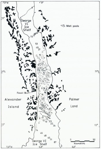
George VI Sound is a channel separating Alexander Island from Palmer Land (Fig. 1). The channel is 500 km long and from 20 to 60 km wide. A depth profile across the northern end showed that the sea bed is shaped roughly like a W; there is a central ridge covered by 400 m of water and flanked by eastern and western troughs 900 and 750 m deep respectively (personal communication from P. Lennon). The steep cliffs and adjacent peaks along the side of the sound define a geological fault, the rocks on the eastern side being metamorphic and igneous whilst those along the western boundary are predominantly sedimentary. All the exposed rock in the area is between 70 and 200 million years old.
Ice movement survey schemes on George VI Ice Shelf.

George VI Sound contains George VI Ice Shelf which is formed by ice flowing westwards off the Palmer Land plateau towards Alexander Island. The ice shelf covers much of the sound and varies from 100 m to 500 m in thickness (Reference SwithinbankSwithinbank, 1968; Reference SmithSmith, 1972). Parts of the ice shelf flood during the summer, making surface travel impossible. Because of flooding and the restricted daylight of winter, surface work on the ice shelf is normally undertaken in spring and autumn.
3. Theory
Relationships involved in the mass balance of ice shelves have been discussed by numerous authors (Reference Wright and PriestleyWright and Priestley, 1922; Reference SwithinbankSwithinbank, 1958; Reference CraryCrary, 1964; Reference BuddBudd, 1966; Reference BehrendtBehrendt, 1970; Reference Thomas and CoslettThomas and Coslett, 1970; Reference ThomasThomas, 1973). We consider the discharge through a section of an ice shelf bounded by flow lines. Coordinate axes arc: x-axis along a flow line at sea-level, z-axis vertically upwards, and y-axis chosen to make the system right-handed.
Nomenclature
Subscripts b and s refer to lower and upper surfaces respectively.
-
q(x) = rate of horizontal mass discharge through a section of width D(x)
-
Ȧ(x) = accumulation rate expressed as mass per unit area (Ȧ b being a bottom freezing rate)
-
U(x) = ice-shelf velocity along a flow line
-
= strain-rate (compression negative)

-
ρ(x, z) = ice-shelf density
-
H(x) = ice thickness (Z s—Zb)
For continuity of mass across a vertical section of width D

where

Away from the hinge zone of an ice shelf, where intense vertical shear may occur, we shall assume U(x) to be independent of z. By also assuming that D is constant with depth, (Equation 2) reduces to
where  is the mean ice density of a vertical section, and the term reduces so that (Equation 1) becomes

Taking D(x)as being invariant with time, this can be expanded as

Now and so that by defining we get

The parameter s can be interpreted as the vertical strain-rate corrected for compaction of firn, where and are the surface horizontal strain-rates.
For steady-state flow of ice through this section, we assume . It then follows that

If the only significant terms are those which affect the bottom flux by 0.1 Mg m−2 a−1 (a value less than the probable measurement error) then taking a typical value for George VI Ice Shelf of U = 200 m a−1 and H = 200 m, significant changes in mean density require

The required value of density gradient is large. Measurements on George VI Ice Shelf indicated that it was unlikely to be reached. Ignoring this term, Equations (3) and (4) reduce to

or for steady-state

Thus parameters which need either to be measured or calculated are those on the right-hand sides of Equations (5) and (6) ; velocity, strain-rates, ice density, surface accumulation rate, ice thickness, and ice thickness gradient. (s > o for horizontal compression, ∂H/∂x < 0 for thinning in the direction of flow and melt rate = –Ȧb.)
4. Field Measurements
Several hundred aluminium stakes were set up on George VI Ice Shelf in networks of varying shape and size. Velocity, strain, and accumulation rates were measured at these stakes over a period of several years. The results were combined with ice thicknesses from airborne radio echo-sounding and with density measurements from surface levelling, from bore holes, and from shallow pits.
A. Velocity and strain measurements
Stake networks were measured by conventional survey techniques. Velocities were calculated by various methods (Reference SwithinbankSwithinbank, 1958; Reference WaltonWalton, 1979; Reference Wager, Wager, Doake, Paren and WaltonWager and others, 1980) are shown in Figure 2 together with ice thickness isopleths. Strain-rates were calculated from observations of the relative movement between adjacent stakes. Details of two survey networks on George VI Ice Shelf were reported earlier (Pearson and Rose, in press). A brief description of all the networks is given below.
Ice thickness and velocity on George VI Ice Shelf.

(a) Carse Point. A scheme
This scheme was a conventional trilateration network of 15 stakes, tied into rock points on either side of the sound. Measurements were made over the period 1970–72. Results showed that the ice moves predominantly north-west. Values of principal strains and velocities obtained from eleven triangles were given by Reference Pearson and RosePearson and Rose (in press).
(b) Coal Nunatak. E scheme
This scheme was set up in 1969 and was last measured in 1972. A line of stakes was tied into rock stations at both ends by using a traverse technique. Results showed that the ice shelf was moving north-west, that is to say almost directly across the sound. Strain-rates were obtained at two strain rosettes nearly 10 km apart. Details of this scheme were also given by Reference Pearson and RosePearson and Rose (in press).
(c) Horse Bluff. D scheme
A number of stakes were drilled into the ice shelf across its narrowest point. Rock stations on opposite sides of the sound were used as control, and stake positions were found relative to these by a hybrid traverse/triangulation method. Results showed that the ice was moving slowly with considerable variation in velocity and principal strains. Three measurements were made in 1973 and 1974, yielding velocities to better than ±1 m a−1.
(d) Rosette scheme. R scheme
It was earlier thought that the northern half of George VI Ice Shelf flowed either north or south parallel to the land which flanks it. Velocities observed on the A and E schemes were thus unexpected. Landsat images of the area first became available in 1973 and showed that melt pools on the surface of the ice shelf formed east–west linear patterns that might correspond with flow lines. To Further investigate the flow of the ice shelf, the movement of small isolated networks was measured by repeated resection to surrounding peaks.
Ten strain rosettes were established on flow lines originating from glaciers flowing westwards into the ice shelf from Palmer Land. Two rosettes were put on separate flow lines coming from Millet, Conchie, and Goodenough Glaciers, three rosettes were put on a flow line from Bertram Glacier and one was put on a flow line from Ryder Glacier. Each rosette consisted of four stakes set out so that three stakes were equally spaced at 120° intervals about 1 km from a central stake. The changing internal geometry of each rosette was measured and strains were computed using a strain-tensor technique which also allowed values of rotation and path curvature to be found. Movement was measured by repeated survey from the central stake to six or seven rock stations up to 50 km distant on Palmer Land and Alexander Island. Maps constructed from Landsat mosaics were available for the whole area (Reference Swithinbank, Lane, Peel, Peel, Curtis and BarrettSwithinbank and Lane, [1977]) with the result that positions of the rock stations could be read accurately enough to obtain velocities to better than ±3% (Walton, 1979). The results show quite definitely that the lines of melt pools correspond with flow lines.
(e) Spartan Glacier. BB scheme
Seven stakes were placed up to 4 km from the edge of the ice shelf off Spartan Glacier in late 1974 (Fig. 3). They were intersected from two rock stations set high on the ridges to the north and south of this glacier and provide an interesting study of a zone of highly stressed ice where the ice shelf abuts against Alexander Island. The network was measured four times and velocities are known to better than ± 1.5 m a−1. Results show that the rate of flow is rapidly slowing as the ice approaches Alexander Island.
Velocities and principal strain-rates on the BB scheme off Spartan Glacier.

(f) Ablation point. L scheme
Velocities and strains measured on the ice shelf were found to be of sufficient magnitude that networks measured with only a four-month interval between observations would yield results of acceptable accuracy (±5%). Knowing this, a large triangulation chain was set up in 1975 across the ice shelf between Ablation Point and Gurney Point. The network was not directly linked to any fixed points but was tied in to three previously measured rosettes. It provided detailed information on velocities and strain-rates along a single flow line. Since all internal angles and four base lines were measured, there was considerable redundancy, so the scheme was adjusted using a rigorous least-squares technique to provide “best fit” values of both relative coordinates and velocities. Velocities showed evidence of strong shear across the network and large variations in the surface strain-rate were observed. Velocities of points in the network were measured to ±3 m a−1 and strain-rates to ±1 × 10⁴ a−1 (Fig. 4).
Velocity vectors and principal strain-rates on the L scheme.

(g) Two Step Cliffs. M scheme
This was set up in 1975 along a flow line (Fig. 5). A triangulation chain linked to two strain rosettes was measured to give velocities and strain-rates with an accuracy similar to those of the L scheme. It was hoped that this flow line being further from the open sea would include a zone of possible bottom freezing. Unlike the L scheme, the M scheme appears to lie near the centre of an ice stream with little shear. Vertical strain-rates were computed for each triangle of stakes and values were interpolated for the actual stake positions.
Velocity vectors and principal strain-rates on the M scheme.

B. Ice thickness
The first measurements of ice thickness on George VI Ice Shelf were made in 1966 by airborne radio echo-sounding (Swithinbank, 1968). More detailed coverage was achieved during the 1969–70 and 1971–72 summer seasons. An ice thickness map showing isopachs was drawn from this information in 1973 (Pearson and Rose, in press). Further airborne sounding was carried out during the 1974–75 season before the L and M schemes had been set out. In order to obtain accurate values of ice thickness along these schemes further sounding was carried out in 1976–77 by sledge-borne radio-echo equipment. Traverses were made around the perimeter of the L and M scheme stake networks and the records digitized to give ice thicknesses at horizontal intervals of about 100 m. Thicknesses generally lay in the range 200–500 m.
A computer interpolation technique was devised to calculate ice thickness and the thickness gradient in the direction of flow at particular points. The principle of least squares was used to fit a plane to all ice thickness data points within a given distance of the point at which the gradient was required. Some subjective judgement was needed to choose the best value for this “radius” to avoid over or under smoothing the bottom surface, but a figure of 2.5 km was commonly used.
Because of the small surface slopes on ice shelves, the c. 10 m resolution of the radio echo-sounding equipment used could give rise to a large degree of uncertainty in the thickness gradient. Velocities, strains, densities, and ice thicknesses were usually found to better than ±5% but the probable error in thickness gradient (±0.9 × 10⁻³) may be larger than the gradient itself.
C. Estimation of mean ice-shelf density
The mean density of the ice shelf was estimated in two ways
-
(a) by comparing surface elevation with ice thickness, and
-
(b) by predicting the relationship between depth and density from a knowledge of densities near the surface.
(a) Density from surface elevation and ice thickness
Four level profiles (Fig. 1) were measured on George VI Ice Shelf, two in the central ablation area, one near Carse Point and the other at the southern ice front. Surface elevations were measured with an automatic optical level to give reduced elevations accurate to ±0.2 m. At all except the southern ice front, where a mean sea density of 1.028 Mg m−3 was assumed, surface elevations were tied into measured profiles of sea salinity and temperature. At Moutonnée Lake near Ablation Point (Fig. 1), a layer of fresh water of thickness 35 m was found to overlie a salt water body of average salinity 28‰. At Horse Bluff there was 70 m of fresh water overlying sea-water at 28‰. Ice depths were measured by airborne radio echo-sounding along each of the levelled lines.
Results were computed assuming hydrostatic equilibrium and the average value for each profile is given in Table I.
Surface Elevation Profiles Measured on George VI Ice Shelf

(b) Density from measurements near the surface
Ice cores were obtained to a depth of 10 m at seven points on George VI Ice Shelf. The density of each section of core was determined, samples of denser ice being weighed both in air and in kerosene of known density to minimize the errors. Schytt (1958) suggested that density profiles could be fitted by a function of the form

where K and Z
c are empirical constants, h is the surface elevation, and z is measured upwards from sea-level. Integrating this expression over the top 10 m will give the mean density in terms of Z
c
and K:

The surface density ρ(h) = 0.918 Mg m−3 –K. From a knowledge of the densities in the top 10 m, K and Z c could be evaluated. These were then substituted to yield mean ice-shelf density from the equation

In general,exp so that this expression can be reduced to
Values of were computed for the seven sites and the results are shown in Table II.
Mean Ice-Shelf Densities Computed from 10 m Bore-Hole Data

Mean ice-shelf densities computed in this way show good agreement with densities found by assuming hydrostatic equilibrium. The northernmost bore hole lies nearly half-way between the dense ice found off Moutonnée Lake and the Carse Point level line. The average of the mean densities found in these two regions is 0.890 Mg m−3 which compares well with the density of 0.892 Mg m−3 obtained from using bore-hole data. This suggests that the mean density, which is largely dependent upon the surface regime, may reasonably be predicted elsewhere from similar shallow coring.
D. Accumulation measurements
During the years 1969–76 there were up to 91 snow accumulation stakes on the ice shelf. The length of each stake was measured on as many occasions as possible up to the end of 1976. All data were well supported by density measurements in pits so that snow accumulation results could be reduced to water-equivalent values.
Within the central melt area, ablation or accumulation was found to vary greatly over short distances evidently because summer melt pools affect the drainage and because undulating surfaces encourage the formation of sastrugi. The annual accumulation was taken to be the mean as observed at a small group of stakes, although it was not possible to measure all stakes with equal frequency nor over the same time periods. Frequent measurements made over four years on eight stakes close to Fossil Bluff were used to define a characteristic accumulation curve to interpolate between infrequent measurements on other stakes within the central melt area. Outside this area the accumulation was much larger, so the characteristic curve could not be applied.
A selection of net annual accumulation rates over George VI Ice Shelf are shown in Figure 6. The region between lat. 70° 30′ S. and 72° 00′ S. has a much smaller net balance than the rest of the ice shelf. Two processes may be responsible for this. The first relates to ice temperatures. Figure 7 shows a plot of mean annual accumulation and ice temperatures at 10 m as a function of latitude. Temperatures have been reduced to epoch at 1 November with reference to computed fluctuations at 10 m depth obtained from an analysis of meteorological records at Fossil Bluff (Sanderson, 1978). Although the accumulation rates appear to follow the 10 m temperatures, the relationship may simply be due to the insulation that a snow cover provides during the winter.
Net annual accumulation (× 10−2 Mg m− 2 a− 1) for selected sites on George VI Ice Shelf.
Net annual accumulation and ice temperature at 10 m depth as a function of latitude.

The second process may be related to the topography of the region. The predominant track of depressions is from the north-west over the Bellingshausen Sea and over the high mountains of northern Alexander Island. The mountains receive abundant precipitation but there is a precipitation shadow on the down-wind side. Southern Alexander Island has few mountains and evidently as a result, snow accumulation on George VI Ice Shelf increases south of the 72nd parallel.
Although some of the melt pools on the western side of the ice shelf drain via streams into moulins (personal communication from C. W. M. Swithinbank), most are stagnant; so the winter snow, when it melts, remains in the same place. In this way, despite the intensity of the summer melt, the central zone of the ice shelf enjoys a small net surface accumulation.
5. Discussion
A. Introduction
Measurement of the quantities described in the last section enables the right-hand side of Equations (5) and (6) to be calculated. If the ice shelf is assumed to be in equilibrium these values will correspond with bottom fluxes (Fig. 8).
Selected bottom melting rates computed on the assumption of steady-state behaviour. Observations are represented by an ellipse centred on each point. The major axis of the ellipse is aligned along the flow line and represents the magnitude of the bottom flux. The minor axis represents probable errors. (1 Mg m−2 a−1 ≡ 1.1 m a−1 of ice.)

More detailed results of bottom melting rates along flow lines on the L, M, and BB schemes are shown in Figures 9, 10, and 11 respectively. Also shown in these figures are values of the principal variables in (Equation 6): velocities, ice thicknesses, and vertical strain-rates, to show their influence on bottom melting. For example, the decrease in melt rate with distance from the grounding line for the L and M schemes (Figs 9 and 10) is evidently associated with a corresponding decrease in nearly all the relevant parameters in both cases. The increase in bottom melt rate approaching Alexander Island on the BB scheme can be seen to be associated with the large increase in vertical strain-rate overcoming the decrease in velocity and ice thickness.
Bottom melting rates, velocities, ice thicknesses, and vertical strain-rates for points on the L scheme.

Bottom melting rates, velocities, ice thicknesses, and vertical strain-rates for points on the M scheme.

Bottom melting rates, velocities, ice thicknesses, and vertical strain-rates on a profile approaching Spartan Glacier.

Equations (5) and (6) were derived for a point; in practice measured quantities are averaged over a certain distance or area. The greatest error probably lies in the ice thickness gradients but errors are also introduced by assuming strain-rates and velocities are constant over small areas. Errors in bottom fluxes have been incorporated into Figures 8 to 11 on the basis of estimated errors of each of the measured quantities; they vary therefore from site to site.
B. Thermodynamic behaviour
If it is assumed that George VI Ice Shelf is in equilibrium, then the flux rates shown in Figures 8 to 11 represent bottom melting rates. Although these figures were derived by measuring the kinematic behaviour of the ice shelf, it is the thermal regime at the boundary between the ice and the sea which determines whether melting or freezing occurs and the magnitude of the flux. This dependence can be expressed (Doake, 1976) as
where is the melt rate, ρ the ice density, L the latent heat of fusion of ice, Q
s
the heat flux from the sea into the ice sheet, and Q
i the upward heat flux through the ice shelf at its base.
The heat flux through the ice shelf Q i is determined simply by the temperature gradient in the ice. Normally the upper surface of an ice shelf is colder than the bottom surface so that the upward heat flux is positive. The actual temperature gradient at any point in the ice shelf will depend on the internal velocity and strain fields as well as on the boundary conditions. If in a steady-state situation with no melting or freezing the temperature profile is linear with depth (temperature increasing with depth), then the profile will become convex downwards for bottom melting. Thus an increase in melting rate tends to increase the temperature gradient at the base of the ice shelf, which by increasing the value of Q i lowers the melt rate ((Equation 7)). The ice shelf therefore exerts a stabilizing influence on perturbations in bottom flux rates.
Owing to the thermal inertia of large ice masses, variations in Q i are likely to be small both in time and space. However values of Q s, which are determined by conditions in a boundary layer under the ice shelf, could show a much greater variability. Some of the parameters which may influence Qs and thus bottom flux rates are currents, both tidal and residual, and salinity and temperature profiles. Fresh-water ice will melt at temperatures below its normal freezing point when in contact with saline water above its freezing temperature (Doake, 1976). This process also cools the sea-water and at depth can give waters below their surface freezing point. Sensible heat can be transferred by turbulent flow (Shumskiy and Zotikov, 1963; Gill, 1973). Because the freezing point of sea-water varies with depth, any vertical movement of water will affect the heat available for melting or freezing. The phenomenon of thermohaline convection, which can occur when temperature and salinity gradients have opposing effects on the density of the water, may influence Q s. Thus the variation of bottom melting rates under George VI Ice Shelf may be more related to physical conditions in the water under the ice than to different dynamic regimes in the ice itself.
C. Steady-state ice shelf
We shall attempt to explain the calculated melt-rate pattern assuming that George VI Ice Shelf is in equilibrium. Pearson and Rose (in press) using data from only the A and E schemes put forward two plausible hypotheses to explain their results:
-
(i) That the melt rate was proportional to the travel time from the inland boundary of the ice shelf.
-
(ii) That there was a progressive loss of heat available for melting as the sea-water travelled further beneath the ice.
Although qualitatively the A scheme results appear to suggest that melting rates increase with time afloat, numerical models in which Q s is kept constant and Q i allowed to decrease with time, as the basal temperature gradient decreases, appear unable to reproduce the observed time dependence; the variation in temperature gradient is too small to give the change in melt rate. These calculations cannot be precise without knowing the temperature profile through the ice before it starts floating, so our results must be treated with caution. However, there is a definite trend shown on the L and M schemes of melt rates decreasing with time afloat, contradicting the simple hypothesis suggested for the A scheme.
A glance at Figure 8 is sufficient to show that the increased number of bottom melting values now available cannot fit a picture where melt rates decrease with distance from the ice front. The explanation of the melt-rate pattern is evidently more complicated. There will certainly be a variation of Q i with time afloat and therefore with position, but it is still necessary to have large variations in Q s. Very little is known about the physical properties of the water under George VI Ice Shelf because access is limited to a few sites along the margins of George VI Sound; further work is in progress to obtain data at the ice fronts and through holes bored with a hot water drill.
Salinity and temperature profiles measured at two sites are shown in Figure 12. The Carse Point site lies 50 km from the northern ice front and only 3 km down-stream from the grounding line of an ice stream. Hobbs Pool, 1 km south of Horse Bluff, is 175 km south of the ice front and abuts a small valley glacier at its grounding line.
Profiles of salinity and temperature for Hobbs Pool and Carse Point at the eastern edge of George VI Ice Shelf.

Measurements were made with an Electronic Switchgear Type MC5 salinity bridge on water brought to the surface in a 1.3 1 sampling bottle which incorporated three accurate reversing thermometers. If the water at a given depth is at its freezing point, then ice particles (frazil ice) may exist in equilibrium with the water (Countryman, 1970; Carmack and Foster, 1975). If the ice particles melt in the sample bottle before salinity is measured then an erroneous value, lower than the in situ salinity, is recorded. The sample bottle can have a filter placed over its bottom end to overcome this problem. Another source of error, causing higher in situ salinities to be measured, occurs when ice freezes out of solution onto the sides of the sample bottle during its ascent from depth.
The insulated sample bottle was retrieved as quickly as possible in order to avoid such problems. No ice crystals or ice formation within the bottle were observed. The freezing points were computed according to the formula of Doherty and Kester (1974). The errors in estimating temperature are 0.01 deg and in estimating freezing point 0.05 deg. Measurements of temperature made over a tidal cycle at 200 m depth, close to the bottom of the ice shelf, showed small fluctuations (±0.1 deg). These fluctuations are taken to indicate that there is a regular exchange of water at that depth with flushing of melt water from the ice-shelf bottom. At neither of the sites was an accurate current meter available but no drag could be detected on the sounding bottle from horizontal currents.
Temperatures measured to a lower accuracy in Ablation Lake are well above the freezing point. Admittedly the profiles were shallow (up to 90 m depth) but may indicate warmer water on the west side of George VI Sound.
Little is known of the bathymetry or currents under the ice shelf. The analysis of British Antarctic Survey tidal records (Cartwright, 1980) indicates a general southward movement of water under the ice shelf and a tidal range in the order of 2 m. Current-meter studies at the northern ice front indicate a net southward movement of water although currents measured were small, often less than 0.02 m s−1 (personal communication from P. Lennon). Fuchs (1951, p. 412), at the southern ice front at 23.00 g.m.t., 20 November 1949, noticed a “considerable current” flowing east towards the ice shelf. A tidal prediction based on Cartwright′s analysis of data from Ablation Lake shows that the tide should have been strongly rising at the time.
The conclusion is that until much more is known about the water under George VI Ice Shelf there is no simple explanation for the apparent variation in melt rate that we have found.
D. Non-steady-state behaviour
In this section we consider whether the bottom melting results can be used as evidence for non-steady-state behaviour of George VI Ice Shelf, represented by a variation with time of velocity, ice thickness, density, or the accumulation rate at a point. Unsteady behaviour could be caused, for example, by long-term changes in mass balance of George VI Ice Shelf or of the glaciers that feed it, leading to kinematic waves propagating across the ice shelf (Paterson, 1969).
In order to separate the bottom melting term from the unsteady-state term in (Equation 5), we can make the simplifying assumption that the bottom melt rate is constant in any particular area. If for the L and M schemes the centre of the ice shelf is considered to be in equilibrium, , then the value for the melt rate there can be taken to represent an average for the flow line. Subtracting this value from the calculated melt rates gives values for . Assuming that is negligible, smoothed curves of are shown in Figure 13 as a function of time afloat. If they occur, thickening rates of the order 5 m a−1 might be detectable within a few years. However the assumption of uniform melt rates is too unreal to place much reliance on these values.
Smoothed profiles of the rate of thickening, , for the L and M schemes as a function of time afloat assuming melt rates of 2 m a −1 for the M scheme and 1 m a−1 for the L scheme.

An alternative method of measuring non-steady-state behaviour would be to find areas of accelerating flow (∂U/∂t≠0). Possible increases in velocity at fixed points were found at two sites. At rosette E resections to seven surrounding reference points were made on four occasions to obtain three independent values of velocity. At the BB scheme four measurements were made of the positions of the stakes. Both sites indicate an increasing velocity with time but these small increases are within measurement errors and so cannot be considered conclusive. Problems arise because non-equilibrium behaviour is usually defined by a change of velocity with time at a fixed point in space (Eulerian coordinate system) whereas marker stakes are continuously moving. It is usual for the surface velocity field to be spatially non-uniform, with the result that apparent accelerations of the form U dU/dx will be generated by the normal movement of stakes. Unless measurements are sufficiently dense or there is a long enough interval between measurements to allow a direct comparison between velocities at a given spot, any real acceleration (dU/dt) may be swamped by the apparent acceleration (UdU/dx).
6. Conclusion
The complexity of the flow of George VI Ice Shelf is reflected in the pattern of bottom melt rates. It is not possible to explain the pattern in terms of ice-shelf parameters thus far observed. Thermodynamic considerations suggest that oceanographie conditions in a boundary layer of sea-water in contact with the underside of the ice shelf control the flux rates. Although parts of the ice shelf may be in an unsteady state the evidence is not conclusive. However, if the large number of land glaciers feeding the ice shelf each responds differently to mass-balance changes then a complex pattern of apparent melt rates is to be expected.
Acknowledgements
The field work was carried out in conjunction with various personnel of the British Antarctic Survey especially Roger Tindley, Graham Tourney, Peter Lennon and Tim Stewart. Drs C. W. M. Swithinbank and J. G. Paren gave valuable advice in the formulation of this paper and in particular the authors would like to thank Dr C. S. M. Doake for his guidance and elucidation of the thermodynamic behaviour under ice shelves.


