


1. Introduction
Galaxies are a key building block of the Universe as the primary source of photons at low to high redshifts. Understanding the physical processes that govern their formation and transformation is therefore essential to modern astrophysics and understanding the Universe. As a fundamental quantity in extragalactic astronomy, the star formation rate (SFR) serves as a powerful diagnostic of galactic activity and offers a direct probe of how galaxies build up their stellar mass and evolve over cosmic time (Kennicutt Reference Kennicutt1998; Madau & Dickinson Reference Madau and Dickinson2014; Madau & Fragos Reference Madau and Fragos2017).
SFR is not a quantity that can be measured directly in distant galaxies where individual stars are no longer resolved. Instead, it is inferred from the luminosity of a galaxy at specific wavelengths that trace recent star-forming activity or inferred from spectral energy distribution modelling across a range of wavelengths. These galaxies are typically identified by their strong ultraviolet (UV) emission from young, massive stars and infrared (IR) emission resulting from the re-radiation of starlight by interstellar dust (Kennicutt Reference Kennicutt1998). The most commonly used approaches for estimating SFR consider UV, H
 ${\unicode{x03B1}}$
, IR, and radio wavelength calibrations. While no single method is ideal, extensive research has been devoted to comparing, combining, and correcting these different tracers to improve consistency and accuracy (Hopkins et al. Reference Hopkins, Connolly, Haarsma and Cram2001; Bell Reference Bell2003; Hopkins Reference Hopkins2004; Calzetti et al. Reference Calzetti2007; Kennicutt et al. Reference Kennicutt2009; Hao et al. Reference Hao2011; Davies et al. Reference Davies2016; Davies et al. Reference Davies2017; Brown et al. Reference Brown2017).
${\unicode{x03B1}}$
, IR, and radio wavelength calibrations. While no single method is ideal, extensive research has been devoted to comparing, combining, and correcting these different tracers to improve consistency and accuracy (Hopkins et al. Reference Hopkins, Connolly, Haarsma and Cram2001; Bell Reference Bell2003; Hopkins Reference Hopkins2004; Calzetti et al. Reference Calzetti2007; Kennicutt et al. Reference Kennicutt2009; Hao et al. Reference Hao2011; Davies et al. Reference Davies2016; Davies et al. Reference Davies2017; Brown et al. Reference Brown2017).
A powerful and widely used SFR tracer in the optical regime is the H
 ${\unicode{x03B1}}$
emission line. This line arises from recombination in HII regions that form when UV photons from high mass, short-lived O and B stars ionise surrounding hydrogen gas. Because these stars have lifespans of
${\unicode{x03B1}}$
emission line. This line arises from recombination in HII regions that form when UV photons from high mass, short-lived O and B stars ionise surrounding hydrogen gas. Because these stars have lifespans of
 $\lesssim$
10 Myr, the H
$\lesssim$
10 Myr, the H
 ${\unicode{x03B1}}$
emission line directly traces recent and ongoing star formation (Glazebrook et al. Reference Glazebrook, Blake, Economou, Lilly and Colless1999; Kennicutt & Evans Reference Kennicutt and Evans2012). Like other optical tracers, H
${\unicode{x03B1}}$
emission line directly traces recent and ongoing star formation (Glazebrook et al. Reference Glazebrook, Blake, Economou, Lilly and Colless1999; Kennicutt & Evans Reference Kennicutt and Evans2012). Like other optical tracers, H
 ${\unicode{x03B1}}$
emission is subject to dust attenuation, which necessitates corrections. Accurate measurement of H
${\unicode{x03B1}}$
emission is subject to dust attenuation, which necessitates corrections. Accurate measurement of H
 ${\unicode{x03B1}}$
flux also requires accounting for underlying stellar absorption, where the absorption features from older stellar populations partially fill in the emission line. Correcting for dust attenuation effects depends on the quality of the stellar continuum modelling and subtraction, which can be challenging, particularly in large spectroscopic surveys.
${\unicode{x03B1}}$
flux also requires accounting for underlying stellar absorption, where the absorption features from older stellar populations partially fill in the emission line. Correcting for dust attenuation effects depends on the quality of the stellar continuum modelling and subtraction, which can be challenging, particularly in large spectroscopic surveys.
One of the most widely used tools to infer dust attenuation is the Balmer Decrement, BD = F(H
 ${\unicode{x03B1}}$
)/F(H
${\unicode{x03B1}}$
)/F(H
 ${\unicode{x03B2}}$
), which provides a basis for correcting dust-affected emission line fluxes. Balmer recombination lines are produced in HII regions by young, massive stars (Osterbrock Reference Osterbrock1989). The BD method relies on comparing the observed ratio of Balmer line fluxes (typically H
${\unicode{x03B2}}$
), which provides a basis for correcting dust-affected emission line fluxes. Balmer recombination lines are produced in HII regions by young, massive stars (Osterbrock Reference Osterbrock1989). The BD method relies on comparing the observed ratio of Balmer line fluxes (typically H
 ${\unicode{x03B1}}$
/H
${\unicode{x03B1}}$
/H
 ${\unicode{x03B2}}$
) to the theoretically predicted case B recombination value, with any excess reddening interpreted as dust attenuation. By adopting an extinction law, the wavelength-dependent obscuration can then be quantified and applied to correct emission-line–derived SFRs.
${\unicode{x03B2}}$
) to the theoretically predicted case B recombination value, with any excess reddening interpreted as dust attenuation. By adopting an extinction law, the wavelength-dependent obscuration can then be quantified and applied to correct emission-line–derived SFRs.
A limitation of the BD method is that it typically assumes a uniform dust screen geometry and treats the galaxy as optically thin. In reality, galaxies often exhibit complex, clumpy dust distributions and optically thick central regions, which may lead to underestimates of the true extinction (Calzetti Reference Calzetti2001; Kreckel et al. Reference Kreckel2013; Robertson et al. Reference Robertson2024). Reliable measurements require high signal-to-noise ratios for both the H
 ${\unicode{x03B1}}$
and H
${\unicode{x03B1}}$
and H
 ${\unicode{x03B2}}$
emission lines, which can be challenging, especially for high-redshift or faint galaxy systems. Low S/N in faint emission lines can also introduce significant biases in line-ratio diagnostics (Yuan, Kewley, & Rich Reference Yuan, Kewley and Rich2013). At higher redshifts, detections of both H
${\unicode{x03B2}}$
emission lines, which can be challenging, especially for high-redshift or faint galaxy systems. Low S/N in faint emission lines can also introduce significant biases in line-ratio diagnostics (Yuan, Kewley, & Rich Reference Yuan, Kewley and Rich2013). At higher redshifts, detections of both H
 ${\unicode{x03B1}}$
and H
${\unicode{x03B1}}$
and H
 ${\unicode{x03B2}}$
remain uncommon, with surveys such as HETDEX reporting only three confirmed LAEs at
${\unicode{x03B2}}$
remain uncommon, with surveys such as HETDEX reporting only three confirmed LAEs at
 $z\gtrsim2$
(of which only two have multiple rest-frame optical emission lines detected) (Finkelstein et al. Reference Finkelstein2011).
$z\gtrsim2$
(of which only two have multiple rest-frame optical emission lines detected) (Finkelstein et al. Reference Finkelstein2011).
Radio wavelengths are particularly advantageous in star formation studies due to their ability to penetrate the dust that often obscures UV and optical tracers. Though radio emission is not a direct tracer of star formation activity, its utility as a SFR indicator stems from the well-established correlation between radio and far infrared (FIR) luminosities in star-forming galaxies (Condon Reference Condon1992; Yun, Reddy, & Condon Reference Yun, Reddy and Condon2001; Bell Reference Bell2003; Ivison et al. Reference Ivison2010; Molnár et al. Reference Molnár2021). In addition, radio emission has also been shown to correlate well with dust-corrected H
 ${\unicode{x03B1}}$
luminosities (e.g. Murphy et al. Reference Murphy2011), further reinforcing its connection to recent massive star formation and providing a useful bridge between radio and traditional recombination-line tracers. Previous studies have also directly calibrated H
${\unicode{x03B1}}$
luminosities (e.g. Murphy et al. Reference Murphy2011), further reinforcing its connection to recent massive star formation and providing a useful bridge between radio and traditional recombination-line tracers. Previous studies have also directly calibrated H
 ${\unicode{x03B1}}$
against FIR emission at
${\unicode{x03B1}}$
against FIR emission at
 $z\sim1-2$
, providing important cross-checks on dust-corrected SFR estimates (e.g. Sobral et al. Reference Sobral2013; Ibar et al. Reference Ibar2013). These comparisons highlight both the potential and limitations of using FIR as a reference, motivating the need for refined dust corrections when relying on H
$z\sim1-2$
, providing important cross-checks on dust-corrected SFR estimates (e.g. Sobral et al. Reference Sobral2013; Ibar et al. Reference Ibar2013). These comparisons highlight both the potential and limitations of using FIR as a reference, motivating the need for refined dust corrections when relying on H
 ${\unicode{x03B1}}$
at higher redshift.
${\unicode{x03B1}}$
at higher redshift.
Radio emission has traditionally been studied at
 $1.4$
GHz, though with the advent of many Square Kilometre Array pathfinder telescopes and programmes, this is rapidly expanding to much a broader range of frequencies. Radio emission at frequencies lower than a few GHz is dominated by non-thermal synchrotron radiation produced by cosmic-ray electrons accelerated in supernova remnants. This is an indirect tracer of recent massive star formation over timescales of
$1.4$
GHz, though with the advent of many Square Kilometre Array pathfinder telescopes and programmes, this is rapidly expanding to much a broader range of frequencies. Radio emission at frequencies lower than a few GHz is dominated by non-thermal synchrotron radiation produced by cosmic-ray electrons accelerated in supernova remnants. This is an indirect tracer of recent massive star formation over timescales of
 $\sim$
10–100 Myr (Murphy et al. Reference Murphy2011). At higher frequencies, thermal free-free emission contributes an increasing fraction of the total radio continuum. This emission originates from ionised gas in H II regions and directly traces massive star formation, analogous to H
$\sim$
10–100 Myr (Murphy et al. Reference Murphy2011). At higher frequencies, thermal free-free emission contributes an increasing fraction of the total radio continuum. This emission originates from ionised gas in H II regions and directly traces massive star formation, analogous to H
 ${\unicode{x03B1}}$
or H
${\unicode{x03B1}}$
or H
 ${\unicode{x03B2}}$
. Around
${\unicode{x03B2}}$
. Around
 $\sim$
30 GHz, the free-free and synchrotron components become comparable in strength (Condon Reference Condon1992).
$\sim$
30 GHz, the free-free and synchrotron components become comparable in strength (Condon Reference Condon1992).
Contamination from AGN can complicate interpretations, necessitating careful source classification (Cowley et al. Reference Cowley2016). Once dust extinction is accounted for, H
 ${\unicode{x03B1}}$
has relatively few assumptions for the conversion to SFR (i.e. recent star formation history and initial mass function) and thus is less susceptible to systematic errors than some tracers. The relative insensitivity of radio emission to dust obscuration raises the possibility that statistical measurements of star formation in the radio could be used to inform or calibrate dust corrections for optical tracers like H
${\unicode{x03B1}}$
has relatively few assumptions for the conversion to SFR (i.e. recent star formation history and initial mass function) and thus is less susceptible to systematic errors than some tracers. The relative insensitivity of radio emission to dust obscuration raises the possibility that statistical measurements of star formation in the radio could be used to inform or calibrate dust corrections for optical tracers like H
 ${\unicode{x03B1}}$
, but this approach has not been comprehensively explored.
${\unicode{x03B1}}$
, but this approach has not been comprehensively explored.
The aim of this study is to develop a new approach for dust obscuration correction in measurements of star formation, particularly at high redshifts where traditional methods become increasingly challenging (Sanders et al. Reference Sanders2024). Dust correction is likely the single dominant source of uncertainty at intermediate redshifts
 $1 \lt z\lt 5$
, which means an empirical SFR based dust correction method, that is dependent on luminosity and redshift, could have great impact in this epoch. This need is motivated by the frequent absence of wavelength coverage and/or sufficient signal-to-noise to perform Balmer decrement–based corrections for individual galaxies in current deep surveys (e.g. Reddy et al. Reference Reddy, Topping, Sanders, Shapley and Brammer2023; Matharu et al. Reference Matharu2023; Shapley et al. Reference Shapley, Sanders, Reddy, Topping and Brammer2023). To address this limitation, we exploit the well-established relationship between H
$1 \lt z\lt 5$
, which means an empirical SFR based dust correction method, that is dependent on luminosity and redshift, could have great impact in this epoch. This need is motivated by the frequent absence of wavelength coverage and/or sufficient signal-to-noise to perform Balmer decrement–based corrections for individual galaxies in current deep surveys (e.g. Reddy et al. Reference Reddy, Topping, Sanders, Shapley and Brammer2023; Matharu et al. Reference Matharu2023; Shapley et al. Reference Shapley, Sanders, Reddy, Topping and Brammer2023). To address this limitation, we exploit the well-established relationship between H
 ${\unicode{x03B1}}$
and radio tracers in the local Universe (e.g. Hopkins et al. Reference Hopkins, Connolly, Haarsma and Cram2001, Ahmed et al. submitted). This link provides a pathway to extend dust-correction techniques to the early Universe, where the James Webb Space Telescope (JWST) has significantly expanded our ability to probe star-forming galaxies, enabling detailed observations of systems out to redshifts
${\unicode{x03B1}}$
and radio tracers in the local Universe (e.g. Hopkins et al. Reference Hopkins, Connolly, Haarsma and Cram2001, Ahmed et al. submitted). This link provides a pathway to extend dust-correction techniques to the early Universe, where the James Webb Space Telescope (JWST) has significantly expanded our ability to probe star-forming galaxies, enabling detailed observations of systems out to redshifts
 $z \gt 10$
(Pontoppidan et al. Reference Pontoppidan2022). Such surveys offer a vital dataset for studying the evolution of star formation through H
$z \gt 10$
(Pontoppidan et al. Reference Pontoppidan2022). Such surveys offer a vital dataset for studying the evolution of star formation through H
 ${\unicode{x03B1}}$
emission at the earliest epochs, provided that robust obscuration corrections can be established. To this end, we adopt a model for luminosity dependent obscuration anchored in the local relation, and progressively reduce its strength with redshift, using the cosmic star formation history as a constraint. This approach allows us to infer the likely redshift dependence of luminosity dependent obscuration in H
${\unicode{x03B1}}$
emission at the earliest epochs, provided that robust obscuration corrections can be established. To this end, we adopt a model for luminosity dependent obscuration anchored in the local relation, and progressively reduce its strength with redshift, using the cosmic star formation history as a constraint. This approach allows us to infer the likely redshift dependence of luminosity dependent obscuration in H
 ${\unicode{x03B1}}$
, thereby enabling physically motivated corrections applicable to the earliest galaxies.
${\unicode{x03B1}}$
, thereby enabling physically motivated corrections applicable to the earliest galaxies.
The layout of this paper is as follows. In Section 2 the radio and optical data used in order to fit a SFR tracer relationship is introduced. In this same section a compilation of published H
 ${\unicode{x03B1}}$
luminosity function results are presented, along with details on dust correction removal and IMF conversion where needed. Then in Section 3 the novel approach to dust correction for H
${\unicode{x03B1}}$
luminosity function results are presented, along with details on dust correction removal and IMF conversion where needed. Then in Section 3 the novel approach to dust correction for H
 ${\unicode{x03B1}}$
luminosities is introduced and applied to published work. The results of this new dust correction are fitted for their luminosity function (LF) and star formation rate density (SFRD) evolution in Section 4. Throughout we assume cosmological parameters of
${\unicode{x03B1}}$
luminosities is introduced and applied to published work. The results of this new dust correction are fitted for their luminosity function (LF) and star formation rate density (SFRD) evolution in Section 4. Throughout we assume cosmological parameters of
 $H_0=70\,$
km s
$H_0=70\,$
km s
 $^{-1}$
Mpc
$^{-1}$
Mpc
 $^{-1}$
,
$^{-1}$
,
 $\Omega_M=0.3$
,
$\Omega_M=0.3$
,
 $\Omega_\Lambda=0.7$
, and
$\Omega_\Lambda=0.7$
, and
 $\Omega_{{k}} = 0$
, a convenient approximation to recent measurements (e.g. Planck Collaboration et al. Reference Collaboration2016). Adopting more precise cosmological values does not change any of our analysis measurably. We adopt a Chabrier IMF, converting other published results to this IMF as needed.
$\Omega_{{k}} = 0$
, a convenient approximation to recent measurements (e.g. Planck Collaboration et al. Reference Collaboration2016). Adopting more precise cosmological values does not change any of our analysis measurably. We adopt a Chabrier IMF, converting other published results to this IMF as needed.
2. Data
This analysis requires data from multiple catalogues to create a multiwavelength study of star forming galaxies (SFGs) that connects the obscured H
 ${\unicode{x03B1}}$
SFR tracer to the unobscured radio SFR tracer, for the same set of sources over a large enough coverage for a statistical study. We use early science radio data from the Evolutionary Map of the Universe (EMU, Norris et al. Reference Norris2011, Reference Norris2021; Hopkins et al. Reference Hopkins2025), focusing on the G23 field. This dataset is integrated with far ultraviolet (FUV) and FIR data from the Galaxy and Mass Assembly (GAMA) survey (Driver et al. Reference Driver2009, Reference Driver2011, Reference Driver2022; Liske et al. Reference Liske2015). The combined EMU-GAMA data, within a redshift range of
${\unicode{x03B1}}$
SFR tracer to the unobscured radio SFR tracer, for the same set of sources over a large enough coverage for a statistical study. We use early science radio data from the Evolutionary Map of the Universe (EMU, Norris et al. Reference Norris2011, Reference Norris2021; Hopkins et al. Reference Hopkins2025), focusing on the G23 field. This dataset is integrated with far ultraviolet (FUV) and FIR data from the Galaxy and Mass Assembly (GAMA) survey (Driver et al. Reference Driver2009, Reference Driver2011, Reference Driver2022; Liske et al. Reference Liske2015). The combined EMU-GAMA data, within a redshift range of
 $0.0\lt z\lt 0.35$
,Footnote
a
is used to compare uncorrected H
$0.0\lt z\lt 0.35$
,Footnote
a
is used to compare uncorrected H
 ${\unicode{x03B1}}$
-based SFRs to radio-derived (1.4 GHz) SFRs, which serve as a dust-unbiased reference. Given that the radio luminosity is unaffected by dust obscuration we adopt it as a proxy for the corrected SFR measure for H
${\unicode{x03B1}}$
-based SFRs to radio-derived (1.4 GHz) SFRs, which serve as a dust-unbiased reference. Given that the radio luminosity is unaffected by dust obscuration we adopt it as a proxy for the corrected SFR measure for H
 ${\unicode{x03B1}}$
. This analysis is then used to correct, or recorrect, for dust obscuration in other published H
${\unicode{x03B1}}$
. This analysis is then used to correct, or recorrect, for dust obscuration in other published H
 ${\unicode{x03B1}}$
luminosity function studies spanning the last
${\unicode{x03B1}}$
luminosity function studies spanning the last
 $\sim$
30 yr.
$\sim$
30 yr.
2.1. Evolutionary Map of the Universe
The EMU is an ongoing radio continuum survey (Hopkins et al. Reference Hopkins2025) aimed at providing a comprehensive view of the Southern sky using the Australian Square Kilometre Array Pathfinder (ASKAP) telescope (Johnston et al. Reference Johnston2007; McConnell et al. Reference McConnell2020). ASKAP employs an array of
 $36\times12\,$
m antennas, covering baselines from 22 to 6 000 m. This configuration enables observations in the 800–1 800 MHz frequency range with an instantaneous bandwidth of 288 MHz. EMU’s use of ASKAP is expected to catalogue approximately 20 million galaxies, providing the most comprehensive atlas of the southern sky, with an angular resolution of
$36\times12\,$
m antennas, covering baselines from 22 to 6 000 m. This configuration enables observations in the 800–1 800 MHz frequency range with an instantaneous bandwidth of 288 MHz. EMU’s use of ASKAP is expected to catalogue approximately 20 million galaxies, providing the most comprehensive atlas of the southern sky, with an angular resolution of
 $\sim$
15′′ FWHM and a sensitivity of roughly
$\sim$
15′′ FWHM and a sensitivity of roughly
 $20\,\unicode{x03BC}$
Jy beam
$20\,\unicode{x03BC}$
Jy beam
 $^{-1}$
.
$^{-1}$
.
For this study, we use EMU early science observations from the GAMA G23 field, (Gürkan et al. Reference Gürkan2022); see also Leahy et al. (Reference Leahy2019) for earlier technical details. The G23 region, centred at
 $\alpha = 23$
h and
$\alpha = 23$
h and
 $\delta = -32^\circ$
, spans an area of
$\delta = -32^\circ$
, spans an area of
 $82.7\,$
deg
$82.7\,$
deg
 $^2$
, with observations at a frequency of 887.5 MHz and a sensitivity of 0.038
$^2$
, with observations at a frequency of 887.5 MHz and a sensitivity of 0.038
 $\unicode{x03BC}$
Jy beam
$\unicode{x03BC}$
Jy beam
 $^{-1}$
. The G23 radio data are matched with the GAMA catalogue to support our analysis.
$^{-1}$
. The G23 radio data are matched with the GAMA catalogue to support our analysis.
2.2. Galaxy and Mass Assembly
The GAMA survey comprises photometric and spectroscopic data across five sky fields (G02, G09, G12, G15, and G23), covering a total area of approximately 280 deg
 $^2$
. Spectroscopic data were obtained using the AAOmega spectrograph on the Anglo-Australian Telescope (AAT), which supports a maximum of 400 fibres and spectral resolution of up to 10 000 (Smith et al. Reference Smith2004; Sharp et al. Reference Sharp2006). Of particular interest for this study is the G23 field that covers 82.7 deg
$^2$
. Spectroscopic data were obtained using the AAOmega spectrograph on the Anglo-Australian Telescope (AAT), which supports a maximum of 400 fibres and spectral resolution of up to 10 000 (Smith et al. Reference Smith2004; Sharp et al. Reference Sharp2006). Of particular interest for this study is the G23 field that covers 82.7 deg
 $^2$
, (
$^2$
, (
 $339^\circ\lt $
RA
$339^\circ\lt $
RA
 $\lt 351^\circ$
,
$\lt 351^\circ$
,
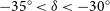 $-35^\circ\lt \delta\lt -30^\circ$
), with a limiting magnitude of
$-35^\circ\lt \delta\lt -30^\circ$
), with a limiting magnitude of
 $i\lt 19.2$
mag at a frequency of 887.5 MHz and was targeted for early science observations from EMU (Gürkan et al. Reference Gürkan2022).
$i\lt 19.2$
mag at a frequency of 887.5 MHz and was targeted for early science observations from EMU (Gürkan et al. Reference Gürkan2022).
We use the latest data from the GAMA Data Release 4 (DR4) in this analysis, accessing three primary catalogues stored in data management units (DMUs) (Bellstedt et al. Reference Bellstedt2020; Driver et al. Reference Driver2022). The first is the StellarMassesv24 table, which includes data on stellar masses, rest-frame photometry, and population synthesis fits across the five survey regions (Taylor et al. Reference Taylor2011). Photometric data for the G23 field are obtained from the gkvInputCatv02 DMU, which integrates data from the European Southern Observatory’s (ESO) Visible and Infrared Survey Telescope for Astronomy (VISTA) Kilo-Degree Infrared Galaxy Public Survey (VIKING; Edge et al. Reference Edge2013) and the ESO VST Kilo Degree Survey (KiDS; Jong et al. Reference Jong2015). GKV (GAMA-KiDS-VIKING), provides multiwavelength photometry spanning from the FUV, using the Galaxy Evolution Explorer (GALEX) space telescope (100–200 nm; Liske et al. Reference Liske2015), to the second WISE band (W2; 4.6
 $\unicode{x03BC}$
m; Wright et al. Reference Wright2010). This DMU is not directly accessed here but is integral to related and ongoing studies of this dataset, including applications such as spectral energy distribution fitting. Emission line fluxes and equivalent width measurements are accessed from the GaussFitSimplev05 DMU (Gordon et al. Reference Gordon2017). This catalogue employs multiple Gaussian fits to enhance accuracy. Previous studies have shown that simpler models yield comparable quantitative results (Ahmed et al. Reference Ahmed2024).
$\unicode{x03BC}$
m; Wright et al. Reference Wright2010). This DMU is not directly accessed here but is integral to related and ongoing studies of this dataset, including applications such as spectral energy distribution fitting. Emission line fluxes and equivalent width measurements are accessed from the GaussFitSimplev05 DMU (Gordon et al. Reference Gordon2017). This catalogue employs multiple Gaussian fits to enhance accuracy. Previous studies have shown that simpler models yield comparable quantitative results (Ahmed et al. Reference Ahmed2024).
2.3. Sample selection
This study focuses on comparing SFR estimators that draw on a diverse set of parameters. To achieve this, GAMA data was cross-matched with that from EMU within the G23 field. In order to achieve this multiwavelength approach, several GAMA catalogues are combined and identical sources were identified based on either spectral or catalogue IDs, leading to a total of 25 762 GAMA sources with emission line and photometric data. A 5-arcsec cross-match with the EMU catalogue, motivated by the cross-match success curves from Ahmed et al. (Reference Ahmed2024), yielded a ‘parent sample’ of 6 633 sources.
The parent sample was refined using several quality assurance markers, resulting in a final sample of 1,036 sources. A detailed explanation of the criteria used is presented here.
The first quality assurance criterion pertains to the Balmer lines, H
 ${\unicode{x03B1}}$
and H
${\unicode{x03B1}}$
and H
 ${\unicode{x03B2}}$
, as well as the NII and OIII emission lines used in the BPT diagnostic. Here a positive detection threshold was established to ensure accurate calculations of luminosities and, consequently, SFRs. Additionally, these emission line fluxes were required to meet a signal-to-noise (S/N) ratio threshold of
${\unicode{x03B2}}$
, as well as the NII and OIII emission lines used in the BPT diagnostic. Here a positive detection threshold was established to ensure accurate calculations of luminosities and, consequently, SFRs. Additionally, these emission line fluxes were required to meet a signal-to-noise (S/N) ratio threshold of
 $\mathrm{S/N}\gt3$
. These cuts are the deepest impact to the sample size but it should guarantee that this work is built on a quality dataset.
$\mathrm{S/N}\gt3$
. These cuts are the deepest impact to the sample size but it should guarantee that this work is built on a quality dataset.
Redshift is necessary for calculating luminosities. Redshift quality is assessed using the parameter
 $nQ \geq 3 $
which corresponds to a redshift of at least 90% confidence (Liske et al. Reference Liske2015). After applying this criterion, relevant equivalent widths were tested for positivity, and a ceiling was applied to the emission line fluxes.
$nQ \geq 3 $
which corresponds to a redshift of at least 90% confidence (Liske et al. Reference Liske2015). After applying this criterion, relevant equivalent widths were tested for positivity, and a ceiling was applied to the emission line fluxes.
Then a flag within the GAMA GaussFitSimple catalogue indicates whether the spectrum used provides the best redshift fit, as some objects have several spectra. The IS_BEST condition is included to further enhance the robustness of the sample.
Finally, the classification of SFGs is done using the standard diagnostic diagram of Reference Baldwin, Phillips and TerlevichBaldwin, Phillips, and Terlevich (BPT, Baldwin, Phillips, & Terlevich Reference Baldwin, Phillips and Terlevich1981; Veilleux & Osterbrock Reference Veilleux and Osterbrock1987). As shown in Figure 1, SFGs are defined as those that fall below the line derived by Kauffmann et al. (2003), forming the basis of our primary sample. Non-star-forming galaxies (nSFGs), identified as those above the theoretical line proposed by Kewley et al. (Reference Kewley, Dopita, Sutherland, Heisler and Trevena2001), are thought to predominantly contain AGN-dominated sources. It is important to note that this classification is not infallible and some AGN sources may still be present within our sample (e.g. Prathap et al. Reference Prathap2024). The region between Kewley et al. (Reference Kewley, Dopita, Sutherland, Heisler and Trevena2001) and Kauffmann et al. (2003) diagnostic lines are composite sources and removed from the sample in addition to the AGN sources to further mitigate possible contamination. It is noted in Sánchez et al. (Reference Sánchez, Muñoz-Tuñón, Almeida, González-Martn and Pérez2025) that BPT-based classifications may overestimate the number of SFGs by up to
 $\sim$
10%. While this level of contamination is unlikely to affect the overall results presented here, it is taken into account when drawing our conclusions. This diagnostic framework enhances the reliability of the SFR calculations by focusing on regions of active star formation.
$\sim$
10%. While this level of contamination is unlikely to affect the overall results presented here, it is taken into account when drawing our conclusions. This diagnostic framework enhances the reliability of the SFR calculations by focusing on regions of active star formation.
The BPT diagram, which uses the [OIII]/H
 ${\unicode{x03B2}}$
and [NII]/H
${\unicode{x03B2}}$
and [NII]/H
 ${\unicode{x03B1}}$
emission line ratios, classifies galaxies as star-forming galaxies (SFGs), active galactic nuclei (AGNs), or composite sources. SFGs, represented by pink stars, lie below the dashed blue Kauffmann line; AGNs, represented by orange circles, are positioned above the solid blue Kewley line; and composite sources, shown as yellow diamonds, are located between the two diagnostic lines. These sources are drawn from the EMU and GAMA catalogues and were processed as described in Section 2.
${\unicode{x03B1}}$
emission line ratios, classifies galaxies as star-forming galaxies (SFGs), active galactic nuclei (AGNs), or composite sources. SFGs, represented by pink stars, lie below the dashed blue Kauffmann line; AGNs, represented by orange circles, are positioned above the solid blue Kewley line; and composite sources, shown as yellow diamonds, are located between the two diagnostic lines. These sources are drawn from the EMU and GAMA catalogues and were processed as described in Section 2.

The selection of our final sample is summarised under the following criteria:
-
1. Positive detection of the H
 ${\unicode{x03B1}}$
and H
${\unicode{x03B2}}$
Balmer lines. (3 931 sources)
${\unicode{x03B1}}$
and H
${\unicode{x03B2}}$
Balmer lines. (3 931 sources) -
2. S/N threshold on the H
${\unicode{x03B1}}$
and H
${\unicode{x03B2}}$
Balmer lines, S/N(H
$\alpha)\gt3$
S/N(H
$\beta)\gt3$
. (1 736 sources) -
3. Redshift quality is checked for nQ
$\geq$
3. (1 736 sources) -
4. Positive detection of the H
${\unicode{x03B1}}$
and H
${\unicode{x03B2}}$
equivalent widths (EW). (1 734 sources) -
5. Ceiling values for H
${\unicode{x03B1}}$
and H
${\unicode{x03B2}}$
Balmer lines are removed. (1 726 sources) -
6. ‘IS_BEST’ flag is true. (1 687 sources)
-
7. SFGs are classified and extracted using the BPT diagram (AGN and composite galaxies are removed from the sample). (1 036 sources)


This results in a final sample of 1 036 SFGs with radio detections in G23.
2.4. Luminosity density compilation
We compiled published H
 ${\unicode{x03B1}}$
luminosities from a broad range of studies (Tresse & Maddox Reference Tresse and Maddox1998; Shioya et al. Reference Shioya2008; Sullivan et al. Reference Sullivan2000; Morioka et al. Reference Morioka2008; Fujita et al. Reference Fujita2003; Stroe & Sobral Reference Stroe and Sobral2015; Pascual et al. Reference Pascual2005; Ly et al. Reference Ly2007; Gallego et al. Reference Gallego, Zamorano, Aragon-Salamanca and Rego1995; Sobral et al. Reference Sobral2013; Hippelein et al. Reference Hippelein2003; Drake et al. Reference Drake2013; Gómez-Guijarro et al. Reference Gómez-Guijarro2016; Yan et al. Reference Yan1999; Hopkins, Connolly, & Szalay Reference Hopkins, Connolly and Szalay2000; Villar et al. Reference Villar2008; Moorwood et al. Reference Moorwood, van der Werf, Cuby and Oliva2000; Hayes, Schaerer, & Östlin Reference Hayes, Schaerer and Östlin2010; Lee et al. Reference Lee2009; Sun et al. Reference Sun2023; Bollo et al. Reference Bollo2023; Covelo-Paz et al. Reference Covelo-Paz2024; Guo et al. Reference Guo2024), spanning approximately 30 yr of research and covering a wide range of redshifts (
${\unicode{x03B1}}$
luminosities from a broad range of studies (Tresse & Maddox Reference Tresse and Maddox1998; Shioya et al. Reference Shioya2008; Sullivan et al. Reference Sullivan2000; Morioka et al. Reference Morioka2008; Fujita et al. Reference Fujita2003; Stroe & Sobral Reference Stroe and Sobral2015; Pascual et al. Reference Pascual2005; Ly et al. Reference Ly2007; Gallego et al. Reference Gallego, Zamorano, Aragon-Salamanca and Rego1995; Sobral et al. Reference Sobral2013; Hippelein et al. Reference Hippelein2003; Drake et al. Reference Drake2013; Gómez-Guijarro et al. Reference Gómez-Guijarro2016; Yan et al. Reference Yan1999; Hopkins, Connolly, & Szalay Reference Hopkins, Connolly and Szalay2000; Villar et al. Reference Villar2008; Moorwood et al. Reference Moorwood, van der Werf, Cuby and Oliva2000; Hayes, Schaerer, & Östlin Reference Hayes, Schaerer and Östlin2010; Lee et al. Reference Lee2009; Sun et al. Reference Sun2023; Bollo et al. Reference Bollo2023; Covelo-Paz et al. Reference Covelo-Paz2024; Guo et al. Reference Guo2024), spanning approximately 30 yr of research and covering a wide range of redshifts (
 $z = 0 - 8$
). The inclusion of high-redshift data from JWST enables a test of our novel dust correction method for H
$z = 0 - 8$
). The inclusion of high-redshift data from JWST enables a test of our novel dust correction method for H
 ${\unicode{x03B1}}$
LFs at the highest observed redshifts.
${\unicode{x03B1}}$
LFs at the highest observed redshifts.
Where possible, we used observed H
 ${\unicode{x03B1}}$
LFs uncorrected for dust obscuration, using published tabulated LFs or binned luminosity density values directly. For datasets published only as figures, we digitised the luminosity function and extracted luminosity density values manually. In cases where only dust-corrected values were available, we reversed the applied corrections detailed in the published work. The most commonly used correction was the scaling factor from Calzetti et al. (Reference Calzetti2000), which we removed to approximate the uncorrected luminosity. In some cases only the average Calzetti correction value was reported, for which we had to assume this in the de-correction across all samples. If insufficient information was available to de-correct dust corrections, the published data was not included in this work. We also noted the IMF assumption used in each study. For any work that included a SFRD calculation adopting the Salpeter (Reference Salpeter1955) IMF, we applied the conversion factor (0.63) to bring all estimates to a common Chabrier (Reference Chabrier2003) IMF following the methodology outlined in Madau & Dickinson (Reference Madau and Dickinson2014). It is also worth noting that all published luminosity functions were fitted with single Schechter functions, and all fit parameters were homogenised to consistent units.
${\unicode{x03B1}}$
LFs uncorrected for dust obscuration, using published tabulated LFs or binned luminosity density values directly. For datasets published only as figures, we digitised the luminosity function and extracted luminosity density values manually. In cases where only dust-corrected values were available, we reversed the applied corrections detailed in the published work. The most commonly used correction was the scaling factor from Calzetti et al. (Reference Calzetti2000), which we removed to approximate the uncorrected luminosity. In some cases only the average Calzetti correction value was reported, for which we had to assume this in the de-correction across all samples. If insufficient information was available to de-correct dust corrections, the published data was not included in this work. We also noted the IMF assumption used in each study. For any work that included a SFRD calculation adopting the Salpeter (Reference Salpeter1955) IMF, we applied the conversion factor (0.63) to bring all estimates to a common Chabrier (Reference Chabrier2003) IMF following the methodology outlined in Madau & Dickinson (Reference Madau and Dickinson2014). It is also worth noting that all published luminosity functions were fitted with single Schechter functions, and all fit parameters were homogenised to consistent units.
3. Dust obscuration correction
The aim of this work is to use the relationship between obscured (H
 ${\unicode{x03B1}}$
) and unobscured (radio) SFRs in order to find a self consistent method for dust correction where spectroscopy or colour correction methods are not applicable. This need comes from the increasing numbers of large rest-frame UV-optical surveys, where dust corrections are difficult to make. Such is the case when the Balmer emission lines are redshifted too far outside the observable wavelength range or have poor S/N (e.g. Reddy et al. Reference Reddy, Topping, Sanders, Shapley and Brammer2023; Matharu et al. Reference Matharu2023; Shapley et al. Reference Shapley, Sanders, Reddy, Topping and Brammer2023). This section details the process we follow to establish a relationship in the SFR between H
${\unicode{x03B1}}$
) and unobscured (radio) SFRs in order to find a self consistent method for dust correction where spectroscopy or colour correction methods are not applicable. This need comes from the increasing numbers of large rest-frame UV-optical surveys, where dust corrections are difficult to make. Such is the case when the Balmer emission lines are redshifted too far outside the observable wavelength range or have poor S/N (e.g. Reddy et al. Reference Reddy, Topping, Sanders, Shapley and Brammer2023; Matharu et al. Reference Matharu2023; Shapley et al. Reference Shapley, Sanders, Reddy, Topping and Brammer2023). This section details the process we follow to establish a relationship in the SFR between H
 ${\unicode{x03B1}}$
and 1.4 GHz radio wavelength tracers. This relationship enables us to convert uncorrected SFRs into dust-corrected values and thereby recover the corresponding inferred intrinsic H
${\unicode{x03B1}}$
and 1.4 GHz radio wavelength tracers. This relationship enables us to convert uncorrected SFRs into dust-corrected values and thereby recover the corresponding inferred intrinsic H
 ${\unicode{x03B1}}$
luminosities. In addition, we explore three alternative models in which the slope of the relationship is varied, providing a means to test its use as a proxy for dust content.
${\unicode{x03B1}}$
luminosities. In addition, we explore three alternative models in which the slope of the relationship is varied, providing a means to test its use as a proxy for dust content.
While both H
 ${\unicode{x03B1}}$
and radio continuum emission are widely used to trace star formation, they probe different physical processes and timescales. H
${\unicode{x03B1}}$
and radio continuum emission are widely used to trace star formation, they probe different physical processes and timescales. H
 ${\unicode{x03B1}}$
emission traces ionising photons from massive stars with lifespans
${\unicode{x03B1}}$
emission traces ionising photons from massive stars with lifespans
 $\lesssim$
10 Myr, providing a snapshot of very recent star formation. In contrast, radio emission which is primarily non-thermal synchrotron radiation from supernova remnants, traces slightly earlier populations of massive stars over longer timescales (
$\lesssim$
10 Myr, providing a snapshot of very recent star formation. In contrast, radio emission which is primarily non-thermal synchrotron radiation from supernova remnants, traces slightly earlier populations of massive stars over longer timescales (
 $\sim$
10–100 Myr; Kennicutt & Evans Reference Kennicutt and Evans2012). The timescale offset means the two tracers may diverge in galaxies with bursty or rapidly changing star formation histories, where the current star formation activity is not well captured by time-averaged radio emission. For example, in recently quenched systems, radio emission can persist for
$\sim$
10–100 Myr; Kennicutt & Evans Reference Kennicutt and Evans2012). The timescale offset means the two tracers may diverge in galaxies with bursty or rapidly changing star formation histories, where the current star formation activity is not well captured by time-averaged radio emission. For example, in recently quenched systems, radio emission can persist for
 $\sim$
100 Myr, leading to an overestimate of the present-day SFR compared to H
$\sim$
100 Myr, leading to an overestimate of the present-day SFR compared to H
 ${\unicode{x03B1}}$
(Arango-Toro et al. Reference Arango-Toro2023).
${\unicode{x03B1}}$
(Arango-Toro et al. Reference Arango-Toro2023).
In galaxies with relatively continuous star formation over these timescales, typical of many star-forming galaxies in the local universe, the tracers are found to correlate well. Duncan et al. (Reference Duncan2020) find that the relationship between radio and H
 ${\unicode{x03B1}}$
SFRs shows no significant evolution out to redshift
${\unicode{x03B1}}$
SFRs shows no significant evolution out to redshift
 $z \sim 2.6$
, providing empirical support for their comparability across a substantial fraction of cosmic history. Cook et al. (Reference Cook2024) demonstrate that calibrating radio-based SFRs requires accounting for the intrinsic timescale sensitivity of each tracer, especially when comparing to IR or UV-optical measures. The full impact of timescale differences across galaxy populations and redshifts remains an open question, and continued observational and theoretical work will be key to understanding where and when these tracers may diverge. The choice of SFR calibration introduces an additional source of uncertainty, as it has been shown to significantly impact both SFR and SFRD estimates, particularly at higher luminosities (e.g. Matthews et al. Reference Matthews, Condon, Cotton and Mauch2021). In this work we adopt the calibrations of Kennicutt (Reference Kennicutt1998) and Bell (Reference Bell2003), though alternative empirical relations could also be explored. With sufficiently broad photometric coverage, spectral energy distribution fitting provides another avenue for deriving consistent SFR estimates.
$z \sim 2.6$
, providing empirical support for their comparability across a substantial fraction of cosmic history. Cook et al. (Reference Cook2024) demonstrate that calibrating radio-based SFRs requires accounting for the intrinsic timescale sensitivity of each tracer, especially when comparing to IR or UV-optical measures. The full impact of timescale differences across galaxy populations and redshifts remains an open question, and continued observational and theoretical work will be key to understanding where and when these tracers may diverge. The choice of SFR calibration introduces an additional source of uncertainty, as it has been shown to significantly impact both SFR and SFRD estimates, particularly at higher luminosities (e.g. Matthews et al. Reference Matthews, Condon, Cotton and Mauch2021). In this work we adopt the calibrations of Kennicutt (Reference Kennicutt1998) and Bell (Reference Bell2003), though alternative empirical relations could also be explored. With sufficiently broad photometric coverage, spectral energy distribution fitting provides another avenue for deriving consistent SFR estimates.
Despite these limitations, a SFR-dependent obscuration correction offers promising potential as a flexible and observationally grounded tool for estimating SFRs, especially in regimes where traditional dust corrections are inaccessible or unreliable. Unlike fixed attenuation laws or colour-based proxies, this method directly links two widely observable quantities: observed H
 ${\unicode{x03B1}}$
luminosity, which is sensitive primarily to the unobscured component of recent star formation (and requires extinction corrections to recover the total), and 1.4 GHz radio luminosity, which is largely insensitive to dust and therefore traces the total star formation (both obscured and unobscured). When calibrated properly, this approach could bridge datasets from UV-optical and radio surveys in a self-consistent way and be deployed in large-scale survey pipelines where full SED fitting is not feasible.
${\unicode{x03B1}}$
luminosity, which is sensitive primarily to the unobscured component of recent star formation (and requires extinction corrections to recover the total), and 1.4 GHz radio luminosity, which is largely insensitive to dust and therefore traces the total star formation (both obscured and unobscured). When calibrated properly, this approach could bridge datasets from UV-optical and radio surveys in a self-consistent way and be deployed in large-scale survey pipelines where full SED fitting is not feasible.
3.1. Radio star formation rates
A common approach in computing radio-based SFRs is to use the flux density at
 $1.4$
GHz. Since the early science EMU catalogue provides data at 888 MHz, we convert to
$1.4$
GHz. Since the early science EMU catalogue provides data at 888 MHz, we convert to
 $1.4$
GHz assuming a spectral indexFootnote
b
of
$1.4$
GHz assuming a spectral indexFootnote
b
of
 $\alpha=-0.7$
. Varying this assumption has a negligible effect on the final result. Once these conversions are made, the radio luminosity can be calculated using:
$\alpha=-0.7$
. Varying this assumption has a negligible effect on the final result. Once these conversions are made, the radio luminosity can be calculated using:
 \begin{equation} L_{1.4\,{\rm GHz}}=\frac{4\pi \times D_L^2 \times S_{1.4}}{({1+z})^{1+\alpha}},\end{equation}
where
 $D_L$
[pc] is the luminosity distance,
$D_L$
[pc] is the luminosity distance,
 $S_{1.4}$
[W Hz
$S_{1.4}$
[W Hz
 $^{-1}$
] is the radio flux, and z is the redshift.
$^{-1}$
] is the radio flux, and z is the redshift.
The radio luminosity is first applied in the calibration derived by Bell (Reference Bell2003), which is based on the correlation between radio and FIR emission (Bell Reference Bell2003; Hopkins et al. Reference Hopkins2003),
 $\text{SFR}_{\textrm{1.4 GHz}}[\mathrm{M}_{\odot}\,\mathrm{yr}^{-1}]=$
 \begin{equation}\begin{cases}\dfrac{L_{\textrm{1.4 GHz}}\,[\textrm{W}\,\textrm{Hz}^{-1}]}{1.81 \times 10^{21}} & \text{for } L \gt L_c, \\[8pt]\dfrac{L_{\textrm{1.4 GHz}}\,[\textrm{W}\,\textrm{Hz}^{-1}]}{[0.1 + 0.9(L/L_c)^{0.3}] \cdot 1.81 \times 10^{21}} & \text{for } L \leq L_c,\end{cases}\end{equation}
where
 $L_c=6.4\times 10^{21} \,\mathrm{W\,Hz}^{-1}$
. Bell uses a step-function-based correction based on a galaxy’s 1.4 GHz luminosity. The luminosity traces non-thermal synchrotron emission from supernova remnants, which correlates with recent star formation. The correlation is strong in star-forming galaxies but less reliable in quiescent galaxies, where the emission may originate from old stars or AGN. The step function in Equation (2), helps avoid overestimating the SFR in such cases. It is worth noting that the Bell (Reference Bell2003) method remains broadly consistent other radio-SFR based calibrations, typically within 20–30%, depending on assumptions such as IMF, radio frequency, and treatment of thermal emission (e.g. Murphy et al. Reference Murphy2011; Delhaize et al. Reference Delhaize2017). As radio wavelengths are unobscured by dust, this SFR acts as the naturally dust corrected SFR.
$L_c=6.4\times 10^{21} \,\mathrm{W\,Hz}^{-1}$
. Bell uses a step-function-based correction based on a galaxy’s 1.4 GHz luminosity. The luminosity traces non-thermal synchrotron emission from supernova remnants, which correlates with recent star formation. The correlation is strong in star-forming galaxies but less reliable in quiescent galaxies, where the emission may originate from old stars or AGN. The step function in Equation (2), helps avoid overestimating the SFR in such cases. It is worth noting that the Bell (Reference Bell2003) method remains broadly consistent other radio-SFR based calibrations, typically within 20–30%, depending on assumptions such as IMF, radio frequency, and treatment of thermal emission (e.g. Murphy et al. Reference Murphy2011; Delhaize et al. Reference Delhaize2017). As radio wavelengths are unobscured by dust, this SFR acts as the naturally dust corrected SFR.
3.2. H
${\unicode{x03B1}}$
star formation rates

The SFRs from H
 ${\unicode{x03B1}}$
emission are derived in order to compare with their radio counterpart. Equations (3) and (4) are first applied to correct for several observational systematics. The H
${\unicode{x03B1}}$
emission are derived in order to compare with their radio counterpart. Equations (3) and (4) are first applied to correct for several observational systematics. The H
 ${\unicode{x03B1}}$
luminosity is then calculated following the methods outlined in Hopkins et al. (Reference Hopkins2003) and Gunawardhana et al. (Reference Gunawardhana2011). Including correcting for stellar absorption and for the aperture losses associated with fibre spectroscopy. We do not apply a dust extinction correction here in order to replicate conditions where such steps are unavailable, thus Balmer Decrement corrections are omitted (Gunawardhana et al. Reference Gunawardhana2013).
${\unicode{x03B1}}$
luminosity is then calculated following the methods outlined in Hopkins et al. (Reference Hopkins2003) and Gunawardhana et al. (Reference Gunawardhana2011). Including correcting for stellar absorption and for the aperture losses associated with fibre spectroscopy. We do not apply a dust extinction correction here in order to replicate conditions where such steps are unavailable, thus Balmer Decrement corrections are omitted (Gunawardhana et al. Reference Gunawardhana2013).
 \begin{multline} L_{H\alpha}\,[\textrm{W}\,\textrm{Hz}^{-1}]=(EW_{H\alpha}+EW_c) \times 10^{-0.4(M_r -34.10)} \\ \times \frac{3 \times 10^{11}}{[6564.61(1+z)]^2}.\end{multline}
The common equivalent width correction (EW
 $_c$
) is assumed to be 1.3
$_c$
) is assumed to be 1.3
 ${\text{A}}$
, (Gunawardhana et al. Reference Gunawardhana2013). The absolute magnitude in the r band (M
${\text{A}}$
, (Gunawardhana et al. Reference Gunawardhana2013). The absolute magnitude in the r band (M
 $_r$
) is provided by the GAMA survey.
$_r$
) is provided by the GAMA survey.
The H
 ${\unicode{x03B1}}$
luminosity is then used to estimate uncorrected SFR as derived by Kennicutt (Reference Kennicutt1998):
${\unicode{x03B1}}$
luminosity is then used to estimate uncorrected SFR as derived by Kennicutt (Reference Kennicutt1998):
 \begin{equation} \text{SFR}_{H\alpha}[{\rm M}_{\odot}\,{\rm yr}^{-1}]= \frac{L_{H\alpha}\,[\textrm{W}\,\textrm{Hz}^{-1}]}{7.9 \times 10^{35}}.\end{equation}
3.3. SFR relationship
Where optical dust correction methods are unavailable or unreliable, the relationship between uncorrected H
 ${\unicode{x03B1}}$
SFR and radio SFR is explored as a means for dust obscuration correction. Once the SFRs for each of our SFGs are calculated, they are compared in Figure 2. The Bell (Reference Bell2003) and Kennicutt (Reference Kennicutt1998) SFR calibrations are adopted here but the calibration choice has minor effects within the overall scatter. To determine the relationship between the SFR estimates, we performed a linear regression using numpy.polyfit with cov=True, which minimises the squared error and returns the covariance matrix for estimating parameter uncertainties. For low SFRs, the 1:1 relationship is adopted as in Hopkins et al. (Reference Hopkins, Connolly, Haarsma and Cram2001), and fitted relationship only begins where data becomes available. The best-fit relation between H
${\unicode{x03B1}}$
SFR and radio SFR is explored as a means for dust obscuration correction. Once the SFRs for each of our SFGs are calculated, they are compared in Figure 2. The Bell (Reference Bell2003) and Kennicutt (Reference Kennicutt1998) SFR calibrations are adopted here but the calibration choice has minor effects within the overall scatter. To determine the relationship between the SFR estimates, we performed a linear regression using numpy.polyfit with cov=True, which minimises the squared error and returns the covariance matrix for estimating parameter uncertainties. For low SFRs, the 1:1 relationship is adopted as in Hopkins et al. (Reference Hopkins, Connolly, Haarsma and Cram2001), and fitted relationship only begins where data becomes available. The best-fit relation between H
 ${\unicode{x03B1}}$
and radio SFRs is shown as the solid line in Figure 2, with the fitted equation given as:
${\unicode{x03B1}}$
and radio SFRs is shown as the solid line in Figure 2, with the fitted equation given as:
 \begin{equation}\log_{10}(\mathrm{SFR}_{\mathrm{H}\alpha,\mathrm{uncorrected}}) = 0.55\log_{10}(\mathrm{SFR}_{1.4\,\mathrm{GHz}}) - 0.22.\end{equation}
The standard errors on the slope and intercept are both
 $\pm$
0.02, as estimated from the diagonal of the covariance matrix.
$\pm$
0.02, as estimated from the diagonal of the covariance matrix.
The relationship between H
 ${\unicode{x03B1}}$
and
${\unicode{x03B1}}$
and
 $1.4$
GHz radio tracers of star formation. Four models are shown: the solid line is the best-fit relation to the local EMU-GAMA SFG sample, while the dashed line marks the 1:1 case, where H
$1.4$
GHz radio tracers of star formation. Four models are shown: the solid line is the best-fit relation to the local EMU-GAMA SFG sample, while the dashed line marks the 1:1 case, where H
 ${\unicode{x03B1}}$
and radio SFRs would be equal, making the 1:1 line the dust free line. The dotted and dot-dashed lines represent proposed interim models. For each model, the redshift interval over which its dust-corrected results align with the published SFRD measurements from Figure 4 is indicated. The truncated equation for each model is shown here for reference but can be seen in full in Table 1. The calibration from Hopkins et al. (Reference Hopkins, Connolly, Haarsma and Cram2001) is shown in orange.
${\unicode{x03B1}}$
and radio SFRs would be equal, making the 1:1 line the dust free line. The dotted and dot-dashed lines represent proposed interim models. For each model, the redshift interval over which its dust-corrected results align with the published SFRD measurements from Figure 4 is indicated. The truncated equation for each model is shown here for reference but can be seen in full in Table 1. The calibration from Hopkins et al. (Reference Hopkins, Connolly, Haarsma and Cram2001) is shown in orange.

Figure 2 is constructed using data from the local Universe,
 $0.0 \lt z \lt 0.35$
,
$0.0 \lt z \lt 0.35$
,
 $0.01\,\mathrm{M}_{\odot}\ \mathrm{dex}^{-1} \lt M \lt 11.69\,\mathrm{M}_{\odot}\,\mathrm{dex}^{-1}$
, and the fit begins at the onset of available data, following the approach of Hopkins et al. (Reference Hopkins, Connolly, Haarsma and Cram2001). To evaluate the applicability of this method across evolving redshift, three additional SFR relationship models are developed. The first, Model 1 (shown as dashed line in Figure 2), assumes no correction–treating the SFRs derived from H
$0.01\,\mathrm{M}_{\odot}\ \mathrm{dex}^{-1} \lt M \lt 11.69\,\mathrm{M}_{\odot}\,\mathrm{dex}^{-1}$
, and the fit begins at the onset of available data, following the approach of Hopkins et al. (Reference Hopkins, Connolly, Haarsma and Cram2001). To evaluate the applicability of this method across evolving redshift, three additional SFR relationship models are developed. The first, Model 1 (shown as dashed line in Figure 2), assumes no correction–treating the SFRs derived from H
 ${\unicode{x03B1}}$
and
${\unicode{x03B1}}$
and
 $1.4$
GHz radio as equivalent. The other two models have slopes that lie between the 1:1 case and our fitted dust-correction model. These models are summarised in Table 1 where the fitted relationship shown in Equation (5) is now referred to as Model 4.
$1.4$
GHz radio as equivalent. The other two models have slopes that lie between the 1:1 case and our fitted dust-correction model. These models are summarised in Table 1 where the fitted relationship shown in Equation (5) is now referred to as Model 4.
Fitted models for the relationship between H
 ${\unicode{x03B1}}$
and 1.4 GHz radio wavelength tracers. Here Model 1 is the 1:1 case with no correction, Model 4 is the fitted relationship to the data and Models 2 and 3 are two intermediate cases that have been chosen to fit SFRD data presented in Section 4.
${\unicode{x03B1}}$
and 1.4 GHz radio wavelength tracers. Here Model 1 is the 1:1 case with no correction, Model 4 is the fitted relationship to the data and Models 2 and 3 are two intermediate cases that have been chosen to fit SFRD data presented in Section 4.

The physical interpretation of these models relates to the inferred level of dust attenuation. The 1:1 line (Model 1) serves as a proxy for a dust-free Universe. In contrast, the fitted relationship (Model 4) reflects the dust content of the local Universe. Models 2 and 3, which fall between Models 1 and 4, therefore represent scenarios with intermediate – that is, reduced–dust attenuation. Our correction method works by inferring the level of dust attenuation from these models and correcting for it accordingly.
To apply this relationship for dust correction, we first convert the H
 ${\unicode{x03B1}}$
luminosities that are uncorrected for dust into uncorrected SFRs using the calibration from Kennicutt (Reference Kennicutt1998), adjusted with the Chabrier IMF correction from Madau & Dickinson (Reference Madau and Dickinson2014). We then determine the corresponding dust-corrected SFR by finding its corresponding radio SFR, dust corrected, based on the model slope applied. The corrected SFR is subsequently converted back into a luminosity by reversing the same SFR calibration. The resulting H
${\unicode{x03B1}}$
luminosities that are uncorrected for dust into uncorrected SFRs using the calibration from Kennicutt (Reference Kennicutt1998), adjusted with the Chabrier IMF correction from Madau & Dickinson (Reference Madau and Dickinson2014). We then determine the corresponding dust-corrected SFR by finding its corresponding radio SFR, dust corrected, based on the model slope applied. The corrected SFR is subsequently converted back into a luminosity by reversing the same SFR calibration. The resulting H
 ${\unicode{x03B1}}$
luminosities are used to fit new luminosity functions, as detailed in Section 4.
${\unicode{x03B1}}$
luminosities are used to fit new luminosity functions, as detailed in Section 4.
An alternative way to express our luminosity- and redshift-dependent calibration from uncorrected H
 ${\unicode{x03B1}}$
SFRs to their radio-derived counterparts is through a multiplicative correction factor (CF). This factor is defined, for each of the three redshift ranges over which our models are applicable, as the ratio of the radio SFR to the uncorrected H
${\unicode{x03B1}}$
SFRs to their radio-derived counterparts is through a multiplicative correction factor (CF). This factor is defined, for each of the three redshift ranges over which our models are applicable, as the ratio of the radio SFR to the uncorrected H
 ${\unicode{x03B1}}$
SFR. Correction factors are computed for four representative uncorrected H
${\unicode{x03B1}}$
SFR. Correction factors are computed for four representative uncorrected H
 ${\unicode{x03B1}}$
luminosities and are presented in Table 2. This quantity effectively parameterises the deviation of each calibration from the one-to-one relation between H
${\unicode{x03B1}}$
luminosities and are presented in Table 2. This quantity effectively parameterises the deviation of each calibration from the one-to-one relation between H
 ${\unicode{x03B1}}$
and radio SFRs. The resulting correction factors clearly indicate that progressively smaller dust corrections are required at higher redshifts.
${\unicode{x03B1}}$
and radio SFRs. The resulting correction factors clearly indicate that progressively smaller dust corrections are required at higher redshifts.
Correction factors converting uncorrected H
 ${\unicode{x03B1}}$
star formation rates to radio-derived star formation rates as a function of redshift and uncorrected H
${\unicode{x03B1}}$
star formation rates to radio-derived star formation rates as a function of redshift and uncorrected H
 ${\unicode{x03B1}}$
luminosity. Correction factors are defined as the ratio
${\unicode{x03B1}}$
luminosity. Correction factors are defined as the ratio
 $\mathrm{SFR}_{\mathrm{1.4\,GHz}}/\mathrm{SFR}_{\mathrm{H}\alpha, \textrm{uncorrected}}$
and are shown for four representative uncorrected H
$\mathrm{SFR}_{\mathrm{1.4\,GHz}}/\mathrm{SFR}_{\mathrm{H}\alpha, \textrm{uncorrected}}$
and are shown for four representative uncorrected H
 ${\unicode{x03B1}}$
luminosities. Luminosities are given in units of
${\unicode{x03B1}}$
luminosities. Luminosities are given in units of
 $10^{36}\,\mathrm{WHz^{-1}}$
.
$10^{36}\,\mathrm{WHz^{-1}}$
.

Published luminosity values, corrected for dust obscuration using the fitted SFR relation from Figure 2 (coloured symbols), along with the corresponding best-fit Schechter functions (dashed line), shown across six redshift bins. Where possible, raw luminosity data from these sources have been used; if necessary, published dust corrections were removed. Our fitted SFR-based dust correction relation (Model 4) was applied instead and new LFs were refitted, where the shaded region depicts the 95% confidence interval from 100 000 MCMC iterations. See Section 2.4 for relevant published H
 ${\unicode{x03B1}}$
luminosity data.
${\unicode{x03B1}}$
luminosity data.

4. Results and analysis
Once we applied our new SFR-based dust correction model to the published luminosities that were either originally uncorrected, or first de-corrected to remove prior extinction estimates, we fit new LFs to the data. Allowing us to compare our approach with existing results and to evaluate how the relationship may vary with redshift by integrating to obtain the SFRD. Using the dust correction from the fitted relationship (Model 4) we present updated LFs in Figure 3. The luminosity values when using the radio-optical SFR based relationship as a dust correction are substantially brighter than in the original LFs, sitting up to two orders of magnitudes higher at all redshifts, compared to the original data.
4.1. Fitting new luminosity functions
The LF,
 $\Phi(L)$
, describes the number of galaxies per unit volume per unit luminosity interval. It is a fundamental statistical tool in observational cosmology that characterises the distribution of galaxy luminosities across the Universe. Since galaxy luminosity is correlated with star formation activity, the LF is often used to study how star formation varies with galaxy population and redshift.
$\Phi(L)$
, describes the number of galaxies per unit volume per unit luminosity interval. It is a fundamental statistical tool in observational cosmology that characterises the distribution of galaxy luminosities across the Universe. Since galaxy luminosity is correlated with star formation activity, the LF is often used to study how star formation varies with galaxy population and redshift.
A widely used analytical form for modelling galaxy LFs in the optical regime is the Schechter function, introduced by Schechter (Reference Schechter1976), and given by:
 \begin{equation}{\unicode{x03D5}}(L)\, dL = {\unicode{x03D5}}^* \left( \frac{L}{L^*} \right)^{\alpha}\exp\!\left(-\frac{L}{L^*}\right) \frac{dL}{L^*},\end{equation}
where
 ${\unicode{x03D5}}^*$
is the normalisation factor for the number density of galaxies,
${\unicode{x03D5}}^*$
is the normalisation factor for the number density of galaxies,
 $L_*$
is the characteristic luminosity where the function transitions from a power-law to an exponential cutoff, and
$L_*$
is the characteristic luminosity where the function transitions from a power-law to an exponential cutoff, and
 ${\unicode{x03B1}}$
is the faint-end slope, describing the abundance of low-luminosity galaxies. We adopt the Schechter function approach to fit the newly corrected luminosity functions.
${\unicode{x03B1}}$
is the faint-end slope, describing the abundance of low-luminosity galaxies. We adopt the Schechter function approach to fit the newly corrected luminosity functions.
To fit Schechter luminosity functions, the luminosity data were divided into six redshift bins spanning
 $z = 0$
– 8. These bins were chosen to group together data with similar redshifts while maintaining a sufficient density of points within each bin to enable statistically robust fitting. The redshift bins are shown in Figure 3, where a reasonably consistent trend is observed within each bin. Although some data points appear to be outliers, they are retained in the fitting process. While the luminosity function refitting process accounts for reported uncertainties, other factors–such as survey area–can influence the results. Larger survey volumes increase the likelihood of detecting rarer, high-luminosity sources, which in turn affects the fitted values of parameters. This becomes especially significant in redshift bins where observational scatter is high.
$z = 0$
– 8. These bins were chosen to group together data with similar redshifts while maintaining a sufficient density of points within each bin to enable statistically robust fitting. The redshift bins are shown in Figure 3, where a reasonably consistent trend is observed within each bin. Although some data points appear to be outliers, they are retained in the fitting process. While the luminosity function refitting process accounts for reported uncertainties, other factors–such as survey area–can influence the results. Larger survey volumes increase the likelihood of detecting rarer, high-luminosity sources, which in turn affects the fitted values of parameters. This becomes especially significant in redshift bins where observational scatter is high.
Each redshift bin was initially fitted with a Schechter function by minimising the residuals, weighted by the uncertainties of the data points. To more reliably quantify the uncertainties in the fitted parameters, the initial solution was refined using a Markov Chain Monte Carlo (MCMC) approach implemented with the Python package emcee, which uses MCMC to efficiently explore parameter space and estimate uncertainties for complex models (Foreman-Mackey et al. Reference Foreman-Mackey, Hogg, Lang and Goodman2012).Footnote c The MCMC was run for 100 000 iterations for each redshift bin. The fitting procedure was repeated independently for the luminosity data corresponding to each of the four models. The best-fit luminosity function parameters for the local SFG SFR dust correction relation (Model 4) are reported in Table 3.
Best-fit parameters of H
 ${\unicode{x03B1}}$
Luminosity function for maximum dust correction model, including reduced chi-squared (
${\unicode{x03B1}}$
Luminosity function for maximum dust correction model, including reduced chi-squared (
 $\chi^2$
) values for each redshift bin.
$\chi^2$
) values for each redshift bin.

4.2. Calculating cosmic star formation rate density
We can derive the cosmic SFRD,
 ${\unicode{x03C1}}_{\text{SFR}}$
, via integration of the luminosity function to compute the luminosity density,
${\unicode{x03C1}}_{\text{SFR}}$
, via integration of the luminosity function to compute the luminosity density,
 ${\unicode{x03C1}}_L$
:
${\unicode{x03C1}}_L$
:
 \begin{equation}{\unicode{x03C1}}_{\text{L}} = \int_{L_{\mathrm{lim}}}^{\infty} L \Phi(L) dL = {\unicode{x03D5}}^* L^* \Gamma(\alpha + 2, L_{\mathrm{lim}} / L^*),\end{equation}
where
 $\Gamma$
is the incomplete gamma function, and
$\Gamma$
is the incomplete gamma function, and
 $L_{\text{lim}}$
is the lower luminosity limit of the integration which is often set by survey completeness (Madau & Dickinson Reference Madau and Dickinson2014). We adopt a value of
$L_{\text{lim}}$
is the lower luminosity limit of the integration which is often set by survey completeness (Madau & Dickinson Reference Madau and Dickinson2014). We adopt a value of
 $L_{\text{lim}}=10^{30}\,\mathrm{W}$
to account for the full range of the data. Through testing of varying lower luminosity limits, there was minimal change in final SFRD value, with up to
$L_{\text{lim}}=10^{30}\,\mathrm{W}$
to account for the full range of the data. Through testing of varying lower luminosity limits, there was minimal change in final SFRD value, with up to
 $\approx$
2% difference when using values up to
$\approx$
2% difference when using values up to
 $L_{\text{lim}}=10^{36.6}\,\mathrm{W}$
and no additional value when integrating to
$L_{\text{lim}}=10^{36.6}\,\mathrm{W}$
and no additional value when integrating to
 $L_{\text{lim}}=10^0\,\mathrm{W}$
.
$L_{\text{lim}}=10^0\,\mathrm{W}$
.
The luminosity density can then be converted into an estimate of the SFRD using a wavelength-dependent SFR calibration factor. These calibrations depend on the IMF and the choice of SFR tracer. For the H
 ${\unicode{x03B1}}$
luminosity we adopt the Kennicutt (Reference Kennicutt1998) calibration, converted to an assumption of a Chabrier IMF:
${\unicode{x03B1}}$
luminosity we adopt the Kennicutt (Reference Kennicutt1998) calibration, converted to an assumption of a Chabrier IMF:
 \begin{equation}{\unicode{x03C1}}_{\text{SFR}}\, (\mathrm{M}_{\odot}\, \mathrm{yr}^{-1}\mathrm{Mpc}^{-3}) = 7.9 \times 10^{-35.24}\,{\unicode{x03C1}}_{\text{L}}\,(\mathrm{W}\,\text{Mpc}^{-3}).\end{equation}
The cosmic SFRD provides a valuable means of tracing the evolution of SFR over cosmic time. The SFRD evolution for each of our four models is presented in Figure 4. This figure compares our results against single or compiled dust-corrected SFRDs from 33 published sources across UV, H
 ${\unicode{x03B1}}$
, IR and Radio wavelengths, see Table A1. As well as the recent dust corrected measurements from Covelo-Paz et al. (Reference Covelo-Paz2024) and Chiang et al. (Reference Chiang, Makiya and Ménard2025).
${\unicode{x03B1}}$
, IR and Radio wavelengths, see Table A1. As well as the recent dust corrected measurements from Covelo-Paz et al. (Reference Covelo-Paz2024) and Chiang et al. (Reference Chiang, Makiya and Ménard2025).
Cosmic SFRDs derived from dust-corrected luminosity functions using each of our four dust correction models, shown in Table 1. These results are compared with recent dust-corrected measurements from Covelo-Paz et al. (Reference Covelo-Paz2024) and Chiang et al. (Reference Chiang, Makiya and Ménard2025) in dashed and dot-dashed lines, respectively. The Madau & Dickinson (Reference Madau and Dickinson2014) relation is also shown in solid grey for comparison. Published dust-corrected star formation rate density (SFRD) values are shown in grey, with markers indicating the observational tracer: UV (circles), H
 ${\unicode{x03B1}}$
(triangles), infrared (squares), and radio (diamonds). The published data is compiled in Table A1.
${\unicode{x03B1}}$
(triangles), infrared (squares), and radio (diamonds). The published data is compiled in Table A1.

Figure 4 demonstrates that the fitted relationship between SFR tracers aligns well with dust-corrected observational data at low redshifts, which is expected given that the relationship was derived from local-Universe data. However, at higher redshifts (
 $z \gt 1$
), the SFRD evolution predicted by the fitted relation exhibits an extreme overestimate that is clearly not well supported by existing measurements.
$z \gt 1$
), the SFRD evolution predicted by the fitted relation exhibits an extreme overestimate that is clearly not well supported by existing measurements.
The less extreme models of Figure 2 demonstrate progressively reduced overestimates at higher redshifts, but also underestimates at the lowest redshifts. The model where no dust correction is applied is the most underestimated but at redshifts
 $z \gt 3.5$
there is H
$z \gt 3.5$
there is H
 ${\unicode{x03B1}}$
data that is well represented by a dustless model. This suggests that an approach to dust correction that evolves with redshift is likely to be necessary over differing redshift ranges.
${\unicode{x03B1}}$
data that is well represented by a dustless model. This suggests that an approach to dust correction that evolves with redshift is likely to be necessary over differing redshift ranges.
For redshifts up to
 $z \approx 0.5$
, the SFR-dependent obscuration correction, calibrated using EMU and GAMA observations over
$z \approx 0.5$
, the SFR-dependent obscuration correction, calibrated using EMU and GAMA observations over
 $0.0 \lt z \lt 0.35$
, produces a cosmic SFRD that is consistent with published values across this range. This results demonstrates that the method can serve as a promising alternative for estimating SFRs in the local Universe, particularly in cases where traditional obscuration corrections based on spectral line diagnostics or galaxy colour methods are unavailable. Such conditions are common in large photometric or radio surveys where emission line data may be incomplete or of low quality (Prathap et al. Reference Prathap2025).
$0.0 \lt z \lt 0.35$
, produces a cosmic SFRD that is consistent with published values across this range. This results demonstrates that the method can serve as a promising alternative for estimating SFRs in the local Universe, particularly in cases where traditional obscuration corrections based on spectral line diagnostics or galaxy colour methods are unavailable. Such conditions are common in large photometric or radio surveys where emission line data may be incomplete or of low quality (Prathap et al. Reference Prathap2025).
Beyond
 $z \sim 1$
, the SFR-dependent obscuration correction increasingly overestimates the SFRD, (Figure 4), with deviations reaching up to two orders of magnitude compared to published work (e.g. Madau & Dickinson Reference Madau and Dickinson2014; Bouwens et al. Reference Bouwens2015). As illustrated in Figure 4, suggesting that the linear relationship between obscured H
$z \sim 1$
, the SFR-dependent obscuration correction increasingly overestimates the SFRD, (Figure 4), with deviations reaching up to two orders of magnitude compared to published work (e.g. Madau & Dickinson Reference Madau and Dickinson2014; Bouwens et al. Reference Bouwens2015). As illustrated in Figure 4, suggesting that the linear relationship between obscured H
 ${\unicode{x03B1}}$
luminosities and 1.4 GHz radio luminosities observed locally does not persist out to redshifts
${\unicode{x03B1}}$
luminosities and 1.4 GHz radio luminosities observed locally does not persist out to redshifts
 $z \sim 7$
.
$z \sim 7$
.
As the redshift increases towards
 $z \approx 1.5$
, the originally calibrated linear relation begins to overestimate the dust correction. This results in a CSFD that is significantly higher than reported values. In contrast, a steeper slope, such as that used in Model 3 (shown in dark orange in Figure 4), produces a markedly better match to the observed data. This suggests that, at progressively increasing redshifts, there is progressively less dust obscuration than seen in the local Universe.
$z \approx 1.5$
, the originally calibrated linear relation begins to overestimate the dust correction. This results in a CSFD that is significantly higher than reported values. In contrast, a steeper slope, such as that used in Model 3 (shown in dark orange in Figure 4), produces a markedly better match to the observed data. This suggests that, at progressively increasing redshifts, there is progressively less dust obscuration than seen in the local Universe.
At redshifts approaching
 $z \approx 3.0$
, we enter the epoch of peak cosmic star formation activity, often referred to as ‘cosmic noon’, (Madau & Dickinson Reference Madau and Dickinson2014). In this regime, we find that the SFR-dependent obscuration correction requires a slope intermediate between that of Model 2 and Model 3 (shown in light and dark orange, respectively, in Figure 4) in order to approximate published values for the SFRD. Implying a transitional phase in the relationship between H
$z \approx 3.0$
, we enter the epoch of peak cosmic star formation activity, often referred to as ‘cosmic noon’, (Madau & Dickinson Reference Madau and Dickinson2014). In this regime, we find that the SFR-dependent obscuration correction requires a slope intermediate between that of Model 2 and Model 3 (shown in light and dark orange, respectively, in Figure 4) in order to approximate published values for the SFRD. Implying a transitional phase in the relationship between H
 ${\unicode{x03B1}}$
and radio luminosities, possibly reflecting a balance between increasing dust production in rapidly evolving galaxies and the onset of more massive, dust-rich systems.
${\unicode{x03B1}}$
and radio luminosities, possibly reflecting a balance between increasing dust production in rapidly evolving galaxies and the onset of more massive, dust-rich systems.
The redshift range above
 $z \approx 3.0$
, is marked by considerable scatter among different SFR tracers, reflecting a lack of consensus across methodologies (Bouwens et al. Reference Bouwens2012; Schenker et al. Reference Schenker2013; Novak et al. Reference Novak2017; Bollo et al. Reference Bollo2023; Covelo-Paz et al. Reference Covelo-Paz2024). The variations may stem from uncertainties in dust content, evolving ISM geometries, dust build up timescales and selection biases inherent in current high-redshift galaxy samples. Recent JWST results also suggest that the emergence of a distinct population of red star-forming galaxies (RedSFGs) at
$z \approx 3.0$
, is marked by considerable scatter among different SFR tracers, reflecting a lack of consensus across methodologies (Bouwens et al. Reference Bouwens2012; Schenker et al. Reference Schenker2013; Novak et al. Reference Novak2017; Bollo et al. Reference Bollo2023; Covelo-Paz et al. Reference Covelo-Paz2024). The variations may stem from uncertainties in dust content, evolving ISM geometries, dust build up timescales and selection biases inherent in current high-redshift galaxy samples. Recent JWST results also suggest that the emergence of a distinct population of red star-forming galaxies (RedSFGs) at
 $3\lt z\lt 4$
may play a role in shaping this behaviour. Tarrasse et al. (Reference Tarrasse2025) identify these RedSFGs as a possible evolutionary link between star-forming and quiescent galaxies, potentially contributing to the observed slope transition in this redshift range. It is worth noting that the Madau & Dickinson (Reference Madau and Dickinson2014) SFRD for
$3\lt z\lt 4$
may play a role in shaping this behaviour. Tarrasse et al. (Reference Tarrasse2025) identify these RedSFGs as a possible evolutionary link between star-forming and quiescent galaxies, potentially contributing to the observed slope transition in this redshift range. It is worth noting that the Madau & Dickinson (Reference Madau and Dickinson2014) SFRD for
 $z\gt3$
aligns almost identically with our Model 1, implying no dust obscuration at all. This is not likely to be physical, given the results noted above, and many others that measure non-negligible obscuration at high redshift.
$z\gt3$
aligns almost identically with our Model 1, implying no dust obscuration at all. This is not likely to be physical, given the results noted above, and many others that measure non-negligible obscuration at high redshift.
In addition to observational factors, the evolution of galaxy metallicities with redshift may also play a role (Panter, Heavens, & Jimenez Reference Panter, Heavens and Jimenez2003; Camps-Fariña et al. Reference Camps-Fariña2022). Lower-metallicity galaxies, which are more common at higher redshifts, produce lower SFRs for a given H
 ${\unicode{x03B1}}$
luminosity. Therefore by applying SFR–luminosity calibrations derived for predominantly solar-metallicity for these high-redshift systems could introduce a systematic bias. While this effect is expected to be smaller than the observed H
${\unicode{x03B1}}$
luminosity. Therefore by applying SFR–luminosity calibrations derived for predominantly solar-metallicity for these high-redshift systems could introduce a systematic bias. While this effect is expected to be smaller than the observed H
 ${\unicode{x03B1}}$
deficit, it may still contribute to the discrepancy; however, quantifying its impact lies beyond the scope of this work.
${\unicode{x03B1}}$
deficit, it may still contribute to the discrepancy; however, quantifying its impact lies beyond the scope of this work.
The fact that neither the steeper nor shallower correction alone accurately reproduces the observed star formation density implies that a single, static obscuration correction is inadequate across this redshift range. Instead, the obscuration characteristics may be evolving more dynamically. This is potentially influenced by variations in star formation modes, ISM geometry (Dalcanton, Yoachim, & Bernstein Reference Dalcanton, Yoachim and Bernstein2004; Holwerda et al. Reference Holwerda2012; Holwerda et al. Reference Holwerda2019), or dust-to-gas ratios. This highlights the need for either a smoothly evolving SFR–based dust calibration or a multi-parametric approach that accounts for additional galaxy properties beyond redshift alone.
4.3. Composite model
These results indicate that the SFR-based dust correction must evolve with redshift to match optical based approaches, no single fit is appropriate. A composite model, constructed by combining the most consistent model across different redshift ranges, is proposed to describe the SFRD evolution. The models are used in with spline fit and then smoothed to create a sample model which is shown in Figure 5.
The SFRD from a spline fit to the step-function model for the SFRD evolution, illustrating the evolving dust correction derived from the fitted relationship between H
 ${\unicode{x03B1}}$
and radio SFR tracers. Here the symbols are the same as in Figure 4. The colours of the spline fit correspond to those in Figure 4 for the model proposed in each redshift range, from the ’local Universe dust content’ scenario of Model 4 to the ’dust-free’ scenario of Model 1. The data points where the spline fit changes model are shown by the overlayed markers, where the marker type represents the model as shown in Figure 4.
${\unicode{x03B1}}$
and radio SFR tracers. Here the symbols are the same as in Figure 4. The colours of the spline fit correspond to those in Figure 4 for the model proposed in each redshift range, from the ’local Universe dust content’ scenario of Model 4 to the ’dust-free’ scenario of Model 1. The data points where the spline fit changes model are shown by the overlayed markers, where the marker type represents the model as shown in Figure 4.

Here we adopt Model 4 in the redshift range
 $0 \lt z \lt 0.5$
, based on the H
$0 \lt z \lt 0.5$
, based on the H
 ${\unicode{x03B1}}$
and Radio SFR relationship in our local Universe which uses observational data in this redshift region. Then a smooth transition to Model 3 is applied for
${\unicode{x03B1}}$
and Radio SFR relationship in our local Universe which uses observational data in this redshift region. Then a smooth transition to Model 3 is applied for
 $0.5 \lt z \lt 1.5$
. Then Model 2 out to redshift
$0.5 \lt z \lt 1.5$
. Then Model 2 out to redshift
 $z \approx 3$
. In this redshift range, the Model should sit somewhere between Model 1 and 2. The redshift ranges over which each model best aligns with the observed cosmic SFRD are annotated in Figure 2. This composite model is expressed as a redshift- and luminosity-dependent correction factor in Equation (9), where
$z \approx 3$
. In this redshift range, the Model should sit somewhere between Model 1 and 2. The redshift ranges over which each model best aligns with the observed cosmic SFRD are annotated in Figure 2. This composite model is expressed as a redshift- and luminosity-dependent correction factor in Equation (9), where
 $\kappa = 7.9\times10^{35}$
is the SFR calibration constant from Kennicutt (Reference Kennicutt1998).
$\kappa = 7.9\times10^{35}$
is the SFR calibration constant from Kennicutt (Reference Kennicutt1998).
 \begin{equation}\mathrm{CF}(L_{\mathrm{H}{\unicode{x03B1}}}, z) =\begin{cases}10^{0.4}\left(\dfrac{L_{\mathrm{H}{\unicode{x03B1}}}}{\kappa}\right)^{-2.22}, & 0 \lt z \lt 0.5, \\[9pt]10^{0.2}\left(\dfrac{L_{\mathrm{H}{\unicode{x03B1}}}}{\kappa}\right)^{-3.33}, & 0.5 \le z \lt 1, \\[9pt]10^{0.08}\left(\dfrac{L_{\mathrm{H}{\unicode{x03B1}}}}{\kappa}\right)^{-6.67}, & 1 \le z \lt 3.\end{cases}\end{equation}
In practice, our prescription for applying a luminosity- and redshift-dependent dust obscuration correction is as follows: first, correct the observed H
 ${\unicode{x03B1}}$
luminosity using Equation (3); next, convert this corrected luminosity into an uncorrected H
${\unicode{x03B1}}$
luminosity using Equation (3); next, convert this corrected luminosity into an uncorrected H
 ${\unicode{x03B1}}$
SFR via Equation (4); finally, apply the correction factor from Equation (9) to obtain a radio-derived SFR that accounts for dust extinction.
${\unicode{x03B1}}$
SFR via Equation (4); finally, apply the correction factor from Equation (9) to obtain a radio-derived SFR that accounts for dust extinction.
The revised model aligns more closely with recent results from Covelo-Paz et al. (Reference Covelo-Paz2024) and Chiang et al. (Reference Chiang, Makiya and Ménard2025), reinforcing the value of a composite approach. In this work, published dust-corrected luminosity functions at
 $z\gt0.35$
are treated as a reference standard. This is not because they represent an absolute ground truth, but because they are derived from well-established, empirically tested correction techniques. Our aim is to demonstrate that the novel radio-based method proposed here could reproduce similarly reliable results. These findings highlight the potential of a radio–optical hybrid framework and suggest that a comprehensive study of SFR-based dust correction methods over cosmic time could be an important step towards developing a SFR based dust correction technique into a robust and widely trusted complement to traditional optical approaches. The development of an evolving SFR-dependent obscuration correction could also offer valuable insights into the physical evolution of dust and gas in galaxies over cosmic time. By examining how the relationship between H
$z\gt0.35$
are treated as a reference standard. This is not because they represent an absolute ground truth, but because they are derived from well-established, empirically tested correction techniques. Our aim is to demonstrate that the novel radio-based method proposed here could reproduce similarly reliable results. These findings highlight the potential of a radio–optical hybrid framework and suggest that a comprehensive study of SFR-based dust correction methods over cosmic time could be an important step towards developing a SFR based dust correction technique into a robust and widely trusted complement to traditional optical approaches. The development of an evolving SFR-dependent obscuration correction could also offer valuable insights into the physical evolution of dust and gas in galaxies over cosmic time. By examining how the relationship between H
 ${\unicode{x03B1}}$
and radio emission changes, one can indirectly track variations in dust content (Driver et al. Reference Driver2018). This model contrasts with the observation that the average dust mass at redshift
${\unicode{x03B1}}$
and radio emission changes, one can indirectly track variations in dust content (Driver et al. Reference Driver2018). This model contrasts with the observation that the average dust mass at redshift
 $z \approx 1$
is approximately a factor of
$z \approx 1$
is approximately a factor of
 $\sim$
3 higher than at
$\sim$
3 higher than at
 $z \approx 0$
. One possible explanation lies in how the spatial distribution of dust within galaxies may change with increasing redshift (Farrah et al. Reference Farrah2008; Pope et al. Reference Pope2008; Casey et al. Reference Casey2014; Farley et al. Reference Farley2025). If regions with higher dust mass do not spatially coincide with areas of strong H
$z \approx 0$
. One possible explanation lies in how the spatial distribution of dust within galaxies may change with increasing redshift (Farrah et al. Reference Farrah2008; Pope et al. Reference Pope2008; Casey et al. Reference Casey2014; Farley et al. Reference Farley2025). If regions with higher dust mass do not spatially coincide with areas of strong H
 ${\unicode{x03B1}}$
emission, then global dust correction methods may introduce biases, leading to an over- or underestimation of the true obscured star formation. The work of Farley et al. (Reference Farley2025) also investigates the scatter of BD among the GAMA sample and how dust mass can further constrain dust quantity in SFGs. Part of the discrepancy may also arise from an increasing contribution of low-luminosity AGN to the radio or FIR emission in galaxies at
${\unicode{x03B1}}$
emission, then global dust correction methods may introduce biases, leading to an over- or underestimation of the true obscured star formation. The work of Farley et al. (Reference Farley2025) also investigates the scatter of BD among the GAMA sample and how dust mass can further constrain dust quantity in SFGs. Part of the discrepancy may also arise from an increasing contribution of low-luminosity AGN to the radio or FIR emission in galaxies at
 $z \gg 1$
, which is explored in Thomson et al. (Reference Thomson2017).
$z \gg 1$
, which is explored in Thomson et al. (Reference Thomson2017).
5. Conclusion
In this work, we have explored the viability of a SFR-dependent obscuration correction based on the empirical relationship between the obscured H
 ${\unicode{x03B1}}$
SFR tracer and the unobscured 1.4 GHz radio SFR tracer. The local SFG H
${\unicode{x03B1}}$
SFR tracer and the unobscured 1.4 GHz radio SFR tracer. The local SFG H
 ${\unicode{x03B1}}$
-radio SFR relationship was initially calibrated as a linear fit over the low-redshift range
${\unicode{x03B1}}$
-radio SFR relationship was initially calibrated as a linear fit over the low-redshift range
 $0.0 \lt z \lt 0.35$
, using EMU and GAMA data, and subsequently applied as a correction to H
$0.0 \lt z \lt 0.35$
, using EMU and GAMA data, and subsequently applied as a correction to H
 ${\unicode{x03B1}}$
luminosities across a broad compilation of published luminosity values. Once our new dust correction method was applied, the new LFs were refitted with Schechter functions. The dust-corrected corrected LFs were then used to estimate the SFRD,
${\unicode{x03B1}}$
luminosities across a broad compilation of published luminosity values. Once our new dust correction method was applied, the new LFs were refitted with Schechter functions. The dust-corrected corrected LFs were then used to estimate the SFRD,
 ${\unicode{x03C1}}_{\text{SFR}}$
, which was compared to other published trends.
${\unicode{x03C1}}_{\text{SFR}}$
, which was compared to other published trends.
At low redshift, the SFR-based dust correction reproduces the cosmic SFRD in good agreement with previous studies. However, at
 $z\gt1$
it significantly overestimates
$z\gt1$
it significantly overestimates
 ${\unicode{x03C1}}_{\mathrm{SFR}}$
, by up to two orders of magnitude. To investigate this discrepancy, we tested three alternative SFR-dependent obscuration correction slopes (models 1–3). The slope, which serves as a proxy for dust content through deviations from a one-to-one H
${\unicode{x03C1}}_{\mathrm{SFR}}$
, by up to two orders of magnitude. To investigate this discrepancy, we tested three alternative SFR-dependent obscuration correction slopes (models 1–3). The slope, which serves as a proxy for dust content through deviations from a one-to-one H
 ${\unicode{x03B1}}$
–radio SFR relation, is found to evolve with redshift. Specifically, the required slope decreases towards earlier epochs.
${\unicode{x03B1}}$
–radio SFR relation, is found to evolve with redshift. Specifically, the required slope decreases towards earlier epochs.
The observed trend towards shallower slopes at earlier epochs indicates a lower average dust content at higher redshift. This result is not inconsistent with previous findings of high obscuration at intermediate and high redshifts (Pérez-González et al. Reference Pérez-González2005; Le Floc’h et al. Reference Le Floc’h2005; Stach et al. Reference Stach2018), which are often attributed to rare, extremely obscured star-forming galaxies that are not represented in local calibrations. The substantial variation observed at high z therefore suggests that more flexible, multi-dimensional calibrations–potentially incorporating galaxy mass, morphology, or spectral energy distribution shape–are required to robustly estimate SFRs across cosmic time. Recent results from the CEERS survey (Bail et al. Reference Bail2024) support this interpretation, linking variations in dust content at high redshift to galaxy structural and stellar population properties, and reinforcing the need for more physically motivated calibrations.
Such an approach holds promise as a practical and physically motivated method for correcting dust attenuation, particularly in cases where direct measurements (such as spectral energy distribution fitting or Balmer decrements) are unavailable. It is shown here that such luminosity dependent corrections for dust would need to decrease in strength with increasing redshift. With further refinement, including a self-consistent and continuous treatment of redshift evolution, a SFR based dust correction method could serve as a valuable tool in the analysis of large survey data and the interpretation of galaxy evolution over cosmic time.
Acknowledgements
We would firstly like to thank Dr. Ian Smail for insightful discussions and helpful suggestions that improved this work.
GAMA is a joint European-Australasian project based around a spectroscopic campaign using the Anglo-Australian Telescope. The GAMA input catalogue is based on data taken from the Sloan Digital Sky Survey and the UKIRT Infrared Deep Sky Survey. Complementary imaging of the GAMA regions is being obtained by a number of independent survey programmes including GALEX MIS, VST KiDS, VISTA VIKING, WISE, Herschel-ATLAS, GMRT, and ASKAP providing UV to radio coverage. GAMA is funded by the STFC (UK), the ARC (Australia), the AAO, and the participating institutions. The GAMA website is http://www.gama-survey.org/.
This scientific work uses data obtained from Inyarrimanha Ilgari Bundara/the Murchison Radio-astronomy Observatory. We acknowledge the Wajarri Yamaji People as the Traditional Owners and native title holders of the Observatory site. The Australian SKA Pathfinder is part of the Australia Telescope National Facility (https://ror.org/05qajvd42) which is managed by CSIRO. Operation of ASKAP is funded by the Australian Government with support from the National Collaborative Research Infrastructure Strategy. ASKAP uses the resources of the Pawsey Supercomputing Centre. Establishment of ASKAP, the Murchison Radio-astronomy Observatory and the Pawsey Supercomputing Centre are initiatives of the Australian Government, with support from the Government of Western Australia and the Science and Industry Endowment Fund.
This paper includes archived data obtained through the CSIRO ASKAP Science Data Archive, CASDA (http://data.csiro.au).
Data availability
Final data products are found at the end of this paper. A coding package that can be used to create luminosity functions using our methodology is being produced and will be made available at https://github.com/jaydewillingham.
Appendix A.
Measurements of SFR Density,
 ${\unicode{x03C1}}_{\text{SFR}}$
[M
${\unicode{x03C1}}_{\text{SFR}}$
[M
 $_{\odot}$
yr
$_{\odot}$
yr
 $^{-1}$
Mpc
$^{-1}$
Mpc
 $^{-3}$
].
$^{-3}$
].

aCalibrated for Chabrier IMF where needed.


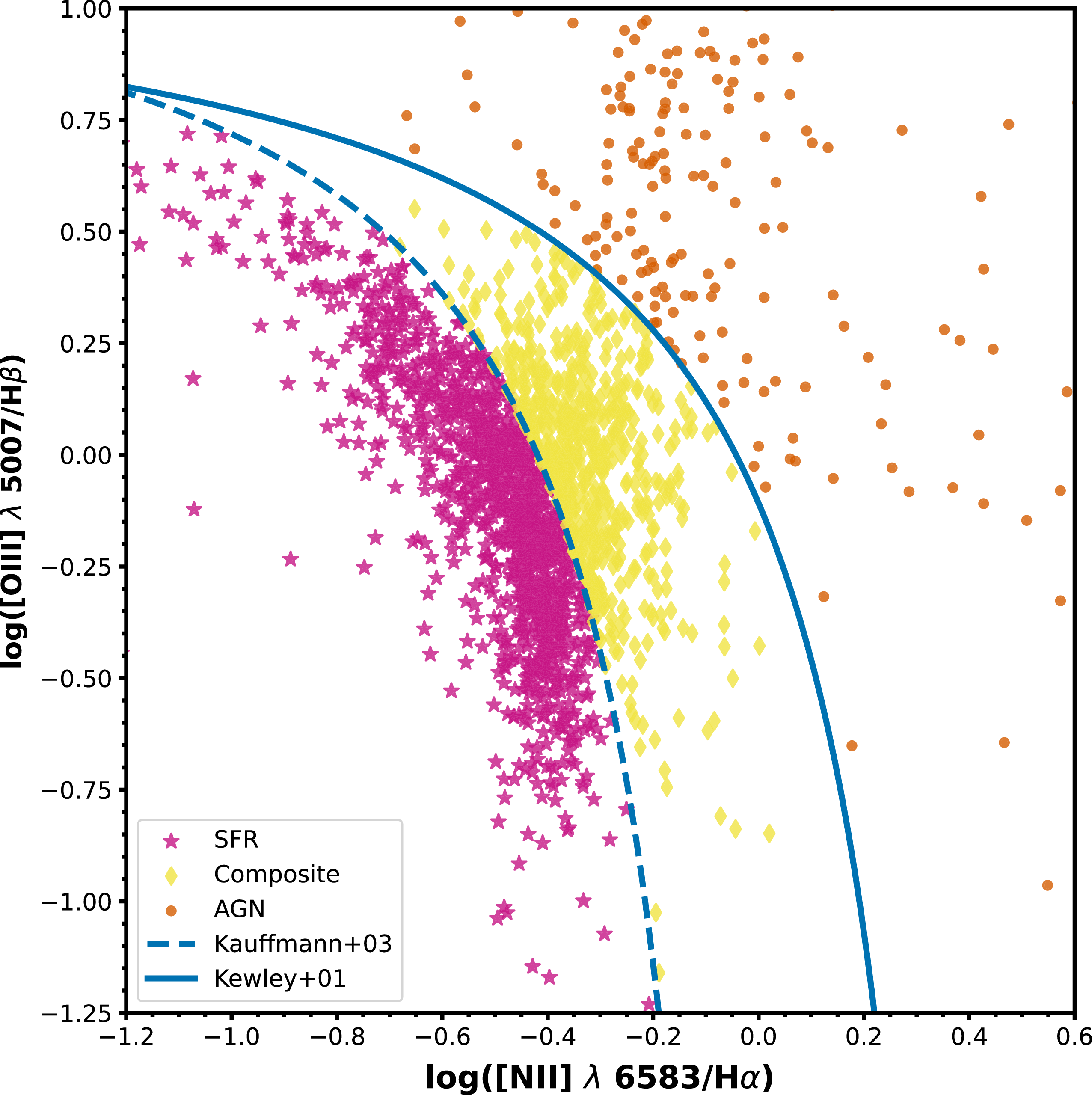


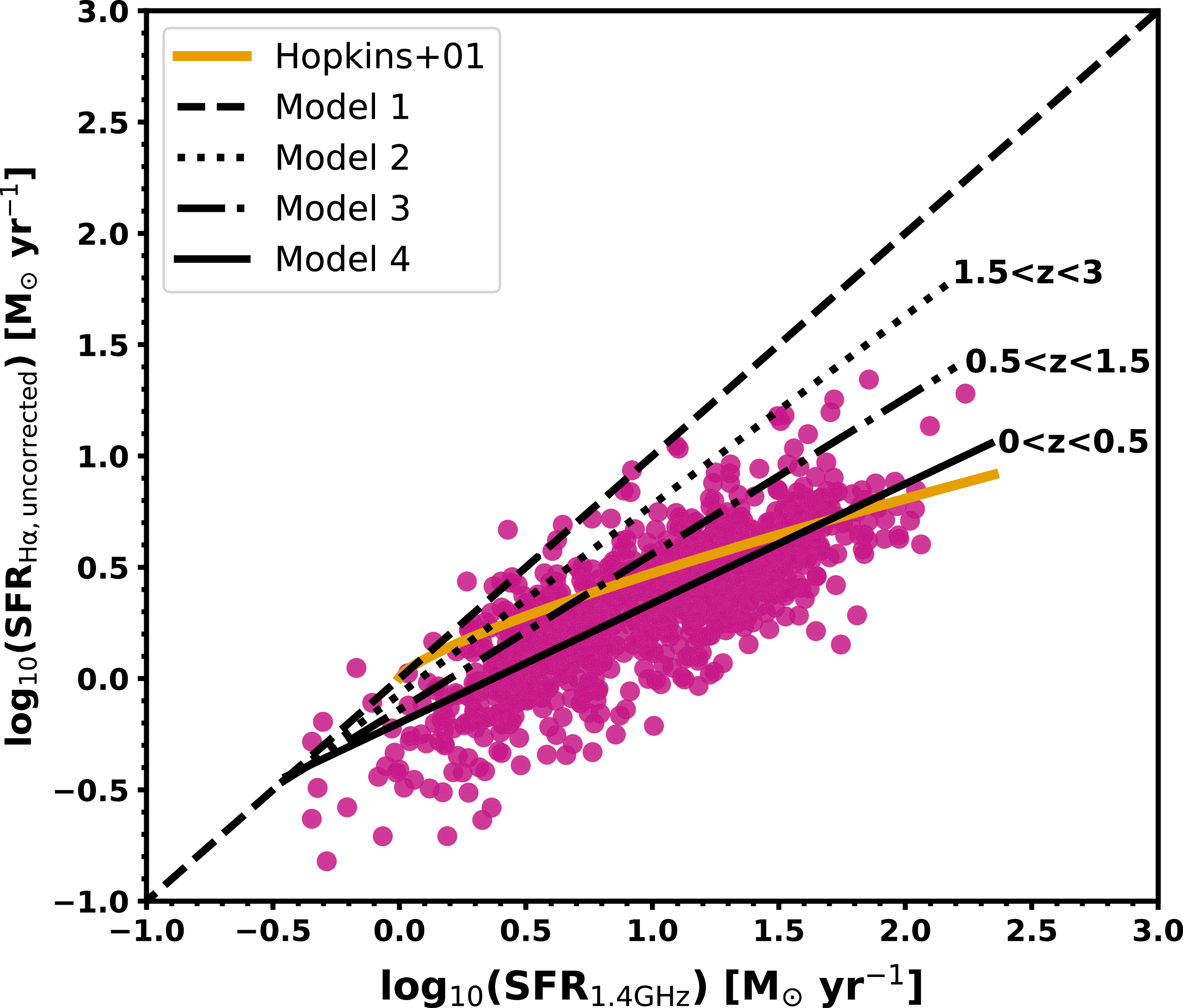


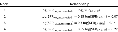

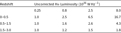


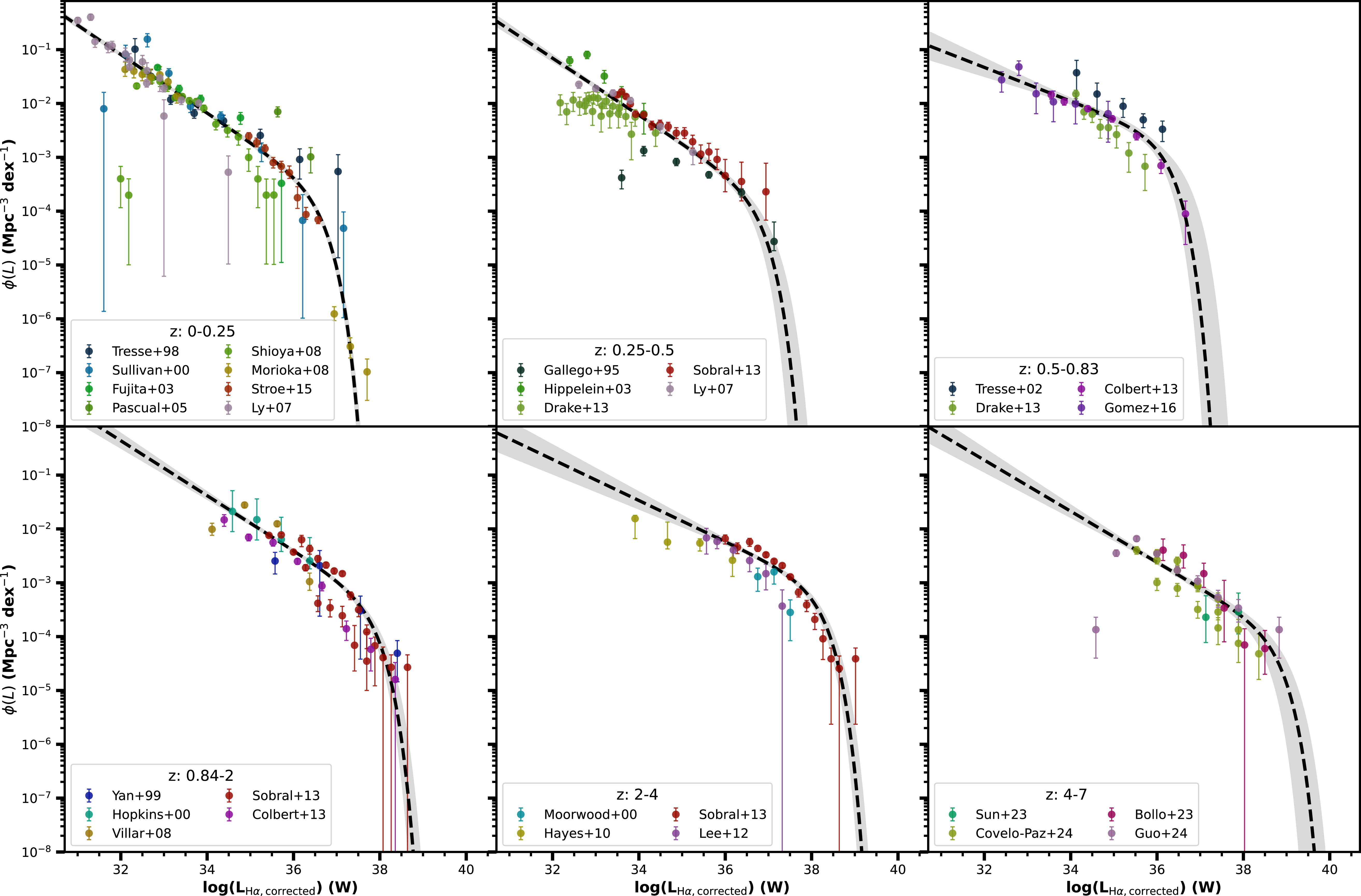

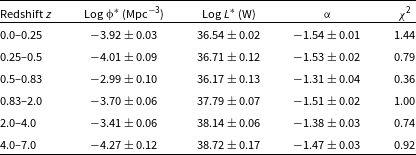


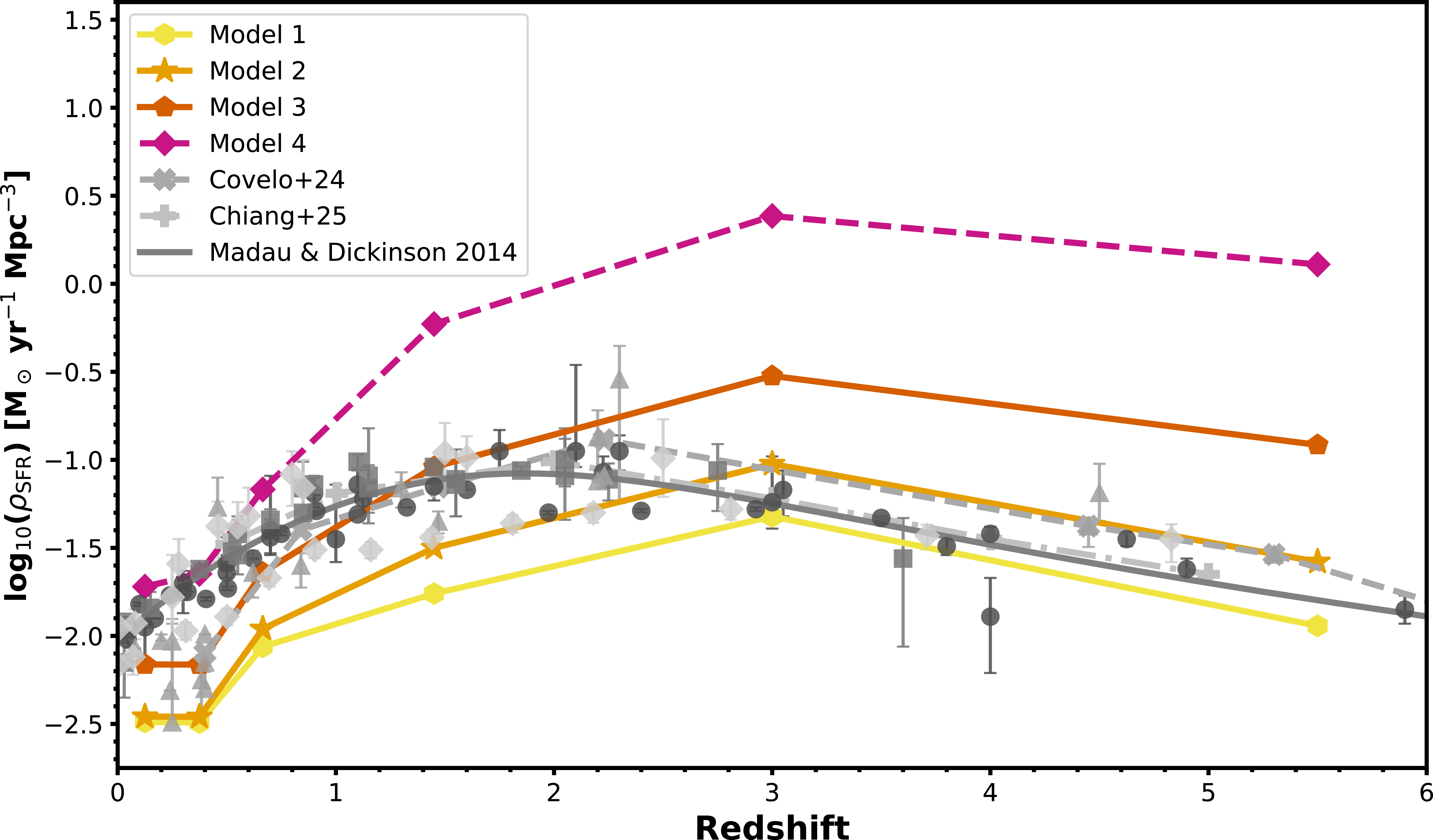

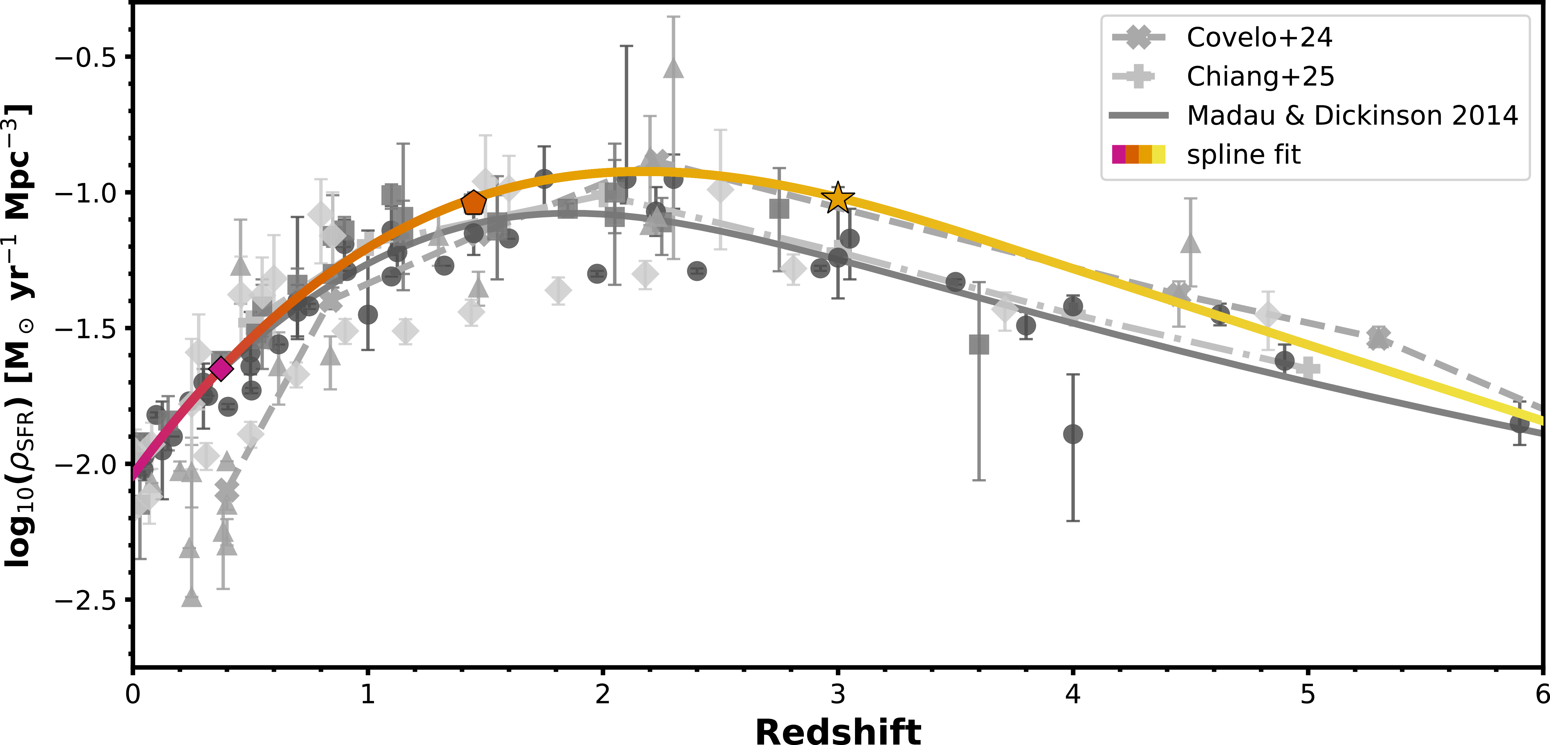


 Open access