


1. Introduction
Markets have always brought people together to trade goods for mutual benefit, but over time their formats have changed — from ancient bazaars and trading posts to the highly complex, computerized exchanges that span the globe today. A natural question arises: can modern tools for human-computer interaction enhance the performance of existing markets?
Human-computer interaction (HCI) has recently developed at the intersection of computer science, cognitive psychology, and design, yielding insights into how people engage with complex digital systems. Yet its application to economic behavior, and in particular to market design, has so far been quite limited. This paper contributes to that emerging application by examining how graphical user interfaces (GUIs) influence market performance.
We investigate various GUIs that implement the standard market format, the continuous double auction (CDA), currently employed in most major financial markets and most laboratory markets. We do so, however, within a very challenging laboratory environment: two-way trade of highly divisible goods with interdependent valuations. That “general equilibrium” or “Edgeworth box” environment is appropriate for our investigation for two reasons. First, it is more representative of field environments than the usual laboratory market environments noted in our survey below, but still is quite familiar to economists. Second, its challenging nature allows more scope for new features to show their strengths and weaknesses. After all, when efficiency approaches 100%, as it does in the simple environments featured in most laboratory market experiments, there is little room to detect improvement.
We hypothesize that highly visual GUIs may help human traders meet the cognitive challenges of our environment and of realistic environments in the field. We assess whether novel features — visual presentation of allocations and valuations (“HeatMap”), geometric display of the order book, and point-and-click order placement — help our human traders find mutually beneficial exchanges. We also assess the impact on overall market performance, especially in terms of exhaustion of gains from trade, price efficiency, and convergence to the contract curve.
Laboratory Markets literature. Our project extends nearly 80 years of laboratory market research. Beginning with oral markets by Chamberlin (Reference Chamberlin1948) and Smith (Reference Smith1962), thousands of studies have confirmed that the continuous double auction (CDA) market format reliably produces efficient outcomes: transaction prices generally converge to the competitive equilibrium price and traders reap most of the potential gains from trade.
Although they extend the original experiments in many imaginative ways, the vast majority of laboratory market studies employ a partial equilibrium environment: the good(s) come in a few indivisible units, each unit having a fixed monetary value or cost for a given trader. Only a handful of laboratory studies to date employ general equilibrium (GE) environments, despite their central role in economic theory since Walras (Reference Walras1874), Edgeworth (Reference Edgeworth1881) and Arrow and Debreu (Reference Arrow and Debreu1954). GE environments are much more cognitively challenging because goods can be finely divisible and their relative marginal valuations can depend on current holdings. Those complications also seem important in the wider world, and so GE economies continue to play a central role in micro theory, macro and finance.Footnote 1
Why, despite their importance, have those challenging GE environments been so seldom studied in the laboratory? As we see it, the main problems concern the human-computer interface. For example, it is easy to design a screen for a partial equilibrium environment that tells a human trader (usually an inexperienced undergraduate) the redemption value (for a buyer) or the opportunity cost (for a seller) of a single unit, or of a few units. It is much more challenging to tell a trader in a general equilibrium environment what a unit (or fraction of a unit, or multiple units) might be worth when the market period is over.
Such challenges have shaped the small existing literature on GE laboratory markets. In their pioneering study, Williams et al. (Reference Williams, Smith, Ledyard and Gjerstad2000) constructed a hybrid environment with subjects trading two coarsely divisible goods against a more finely divisible monetary good. Some subjects were specialized sellers, with essentially partial equilibrium induced cost schedules for one good or the other. As illustrated in Figure 1, their buyers had induced GE preferences but only for small integer-value (0-8) bundles of the two goods. They allow only single unit orders and trades, and only integer prices (in pennies).
Buyer’s interface from Williams et al. (Reference Williams, Smith, Ledyard and Gjerstad2000). Top table induces values for bundles of 1-8 indivisible units of the two goods; current bundle is highlighted. The rest of the screen enables purchase of one unit at a time of each good separately

Subsequent GE studies offered some software improvements. For example, MUDA (multiple unit double auction, Plott and Gray (Reference Plott and Gray1990)) software enabled Anderson et al. (Reference Anderson, Plott, Shimomura and Granat2004) to test Scarf’s (Reference Scarf1960) economy, which features special Leontief preferences over two of three goods. The software accommodates multiple unit orders and trades, facilitating somewhat finer goods divisibility. Specialized sellers were no longer necessary, so theirs was a pure GE exchange economy. Crockett et al. (Reference Crockett, Oprea and Plott2011) and Gillen et al. (Reference Gillen, Hirota, Hsu, Plott and Rogers2021) used MUDA in a similar fashion to examine price divergence in Gale’s (Reference Gale1963) economy. Goeree and Lindsay (Reference Goeree and Lindsay2016) replaced the preference grid (or Profit Table in Figure 1) with color-coded messages suggesting trade directions (e.g. buying a commodity with the numeraire good).
Gjerstad (Reference Gjerstad2013) made further advances in visual interfaces for GE trading. His interface, illustrated in Figure 2, features a dynamic graph and price/quantity grid (“Profit Calculator”) that re-center whenever a trade changes a trader’s current allocation. The interface allows trades of only one indivisible unit at a time, and it accommodates only specialized one-way traders (e.g., the screen shown in Figure 2 is for one-way sellers; an alternative version not shown is for one-way buyers). Gjerstad (Reference Gjerstad2025) uses a very similar interface. Work in progress by B. Williams supplements a payoff grid with a visualization very similiar to the HeatMap feature presented in Figure 5 below.
Experimental interface from Gjerstad (Reference Gjerstad2013). The right panel displays a profit calculator with iso-profit curves and allocation markers, enabling participants to visualize the impact of their trades. The interface features tabular feedback on potential profits

HCI literature. We leverage insights from human-computer interaction (HCI) research to design traders’ graphical user interfaces (GUIs). Our core idea is to use tools from interactive media and videogame design to reduce cognitive load and decision-making frictions, and to leverage human strengths in perceptual and spatial reasoning.
A substantial literature in cognitive psychology and HCI (e.g., Tufte (Reference Tufte1990); Norman (Reference Norman1993); Wickens and Carswell (Reference Wickens and Carswell1995)) suggests that visual-spatial interfaces can improve performance in tasks involving complex decision spaces or multidimensional information. In particular, spatialized displays have been shown to facilitate faster and more accurate decisions compared to equivalent text-based interfaces (Shneiderman, Reference Shneiderman1998; Wickens et al., Reference Wickens, Hollands, Banbury and Parasuraman2013), especially under conditions of time pressure or information overload. Those insights have informed the design of visual analytics tools and dashboards across several domains, but remain underexplored in economics laboratory environments.
Beyond the broader HCI literature, recent work in experimental economics also demonstrates that the visual presentation of information can meaningfully shape decisions. Habib et al. (Reference Habib, Friedman, Crockett and James2017) demonstrate that changes in payoff visualization and presentation framing can meaningfully shift elicited risk preferences in multiple price list tasks, indicating that even subtle interface elements can affect measured behavior. The concluding discussion of Friedman et al. (Reference Friedman, Habib, James and Williams2022) notes recent development by retail financial companies of visual formats to educate customers about returns distributions and to elicit their risk attitudes. Li and Camerer (Reference Ran and Camerer2022) show that, as predicted by computational attention models, stimulus-driven visual salience biases choices in value-based tasks and strategic games, even when visual features are payoff-irrelevant. Similarly, Bose et al. (Reference Bose, Cordes, Nolte, Schneider and Camerer2022) find that the visual salience of points along price charts affects how investors weight past returns, above and beyond statistical properties and standard behavioral models. Together, these studies suggest that visual representation and interface design can alter cognitive processing and economic behavior.
Motivated by these findings, our user interfaces incorporate perceptual cues such as heatmaps of utility landscape, geometric order-book visualizations, and point-and-click trading tools. The general idea is to help human traders reduce their cognitive load and improve their performance in the complex GE environment we study.
Roadmap. The next section collects standard theory concerning the laboratory environment and trading procedures, and introduces our market performance metrics, some of which include novel elements. Section 3 describes our experiment, detailing the user interfaces we will compare and the other treatment variables. Section 4 presents our results. Generally speaking, we find that each of the visual features we investigate seems to improve market performance, sometimes dramatically. Combining both visual and traditional features improves performance in some respects but may impair it in other respects. Section 5 summarizes our results, offers some new perspectives, and suggests directions for future research. Appendix A includes supplementary data analysis, and Appendix B is a copy of the instructions seen by our laboratory subjects.
2. General equilibrium markets
This section presents the general form of the pure exchange economy we investigate, and the specific instances used in our experiment. In that context we define competitive equilibrium and the efficiency metrics used to evaluate market performance. The last subsection reviews the basics of the continuous double auction market format.
2.1. Allocations, preferences and trade
The economies we investigate are populated by traders indexed  $i=1,...,n$. Each trader has her own preferences over non-negative allocations $(x,y) \in \mathbf{R}^2_+$ of two perfectly divisible goods. Those preferences are represented by smooth increasing utility functions $u_i(x,y)$. In the experiment, we induce preferences by paying each human subject a dollar amount proportional to their assigned utility function $u_i$ evaluated at their final post-trade allocation.
Before a period of trade opens, each trader  $i$ is endowed with a non-negative initial allocation $(x_{i0}, y_{i0})$. Each trade is a bilateral exchange between a buyer $i$ who acquires $\Delta x \gt 0$ units of the first good and gives up $\Delta y \gt 0$ units of the second good, and a seller $j\neq i$ who acquires $\Delta y$ and gives up $\Delta x$. The second good is numeraire, so the trade price is $p=\Delta y /\Delta x \gt 0.$ During the trading period, each trader can make several trades according to the rules detailed in Section 2.3 below, each trade changing her allocation by some particular $(\Delta x, -\Delta y)$ when she buys or $(-\Delta x, \Delta y)$ when she sells. At the end of trading period $t$, each trader holds some final allocation $(x_{it}, y_{it})$ and receives payoff $u_i(x_{it}, y_{it}).$
The experiment uses constant elasticity of substitution (CES) utility functions of form
 \begin{equation}
u_{i}(x,y)=c_{i}((a_{i}x)^{r_{i}}+(b_{i}y)^{r_{i}})^{\frac{1}{r_{i}}} \ \ .
\end{equation}
\begin{equation}
u_{i}(x,y)=c_{i}((a_{i}x)^{r_{i}}+(b_{i}y)^{r_{i}})^{\frac{1}{r_{i}}} \ \ .
\end{equation} Each trader knows her own utility function and allocation, and knows that that there are  $n-1=9$ other traders. She knows that the other traders’ utility functions and initial allocations may differ from her own, but knows nothing else about them.
In our experiment, we have 5 type A traders with identical initial allocations  $(x_{i0}, y_{i0}) = (x_A, y_A)$ and utility parameters $(a_i, b_i, c_i, r_i) = (a_A, b_A, c_A, r_A)$. The other 5 traders are type B, with identical initial allocations $(x_{i0}, y_{i0}) = (x_B, y_B)$ and utility parameters
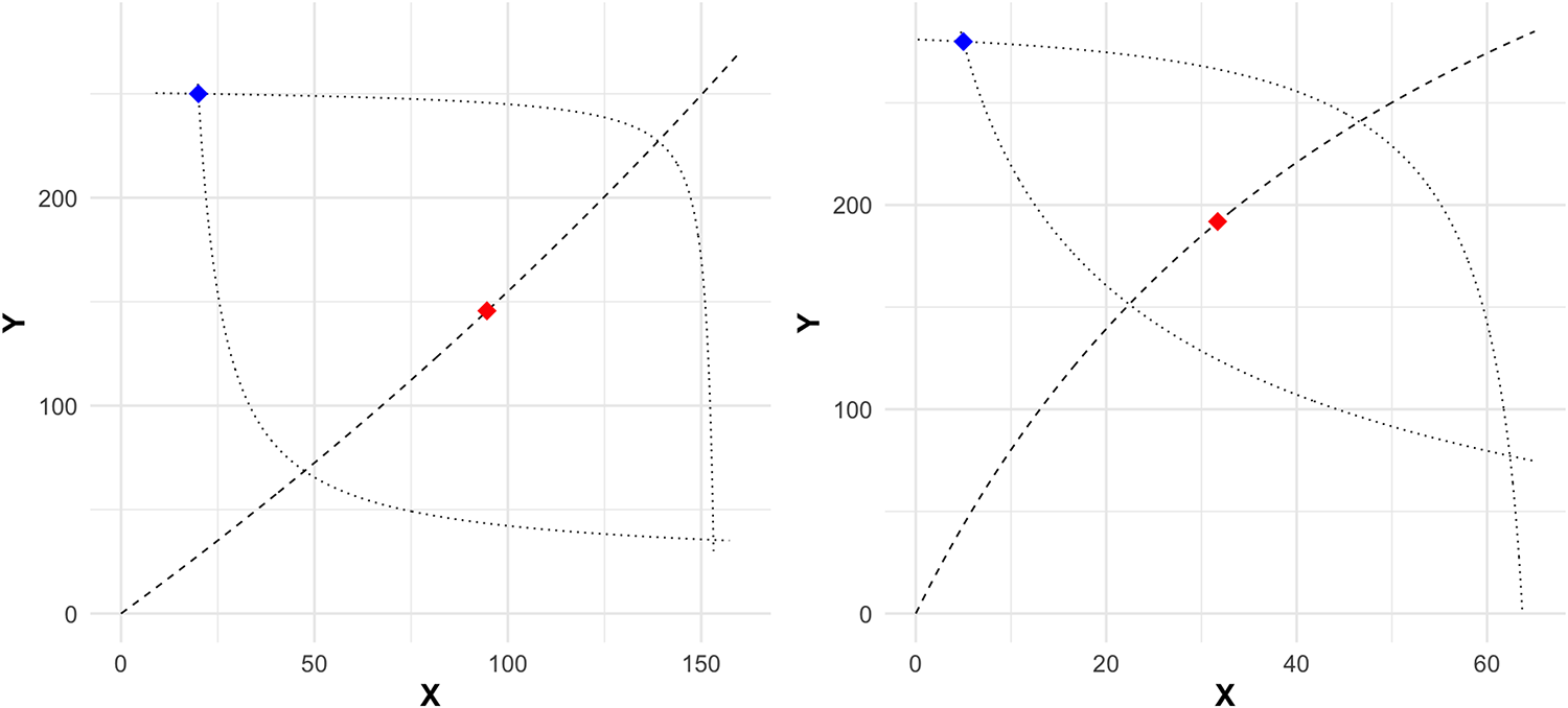
  $(a_i, b_i, c_i, r_i) = (a_B, b_B, c_B, r_B)$. The result is a 5-replica Edgeworth box economy with the underlying parameters given in Table 1; the corresponding Edgeworth boxes are shown in Figure 3. Mainly due to its negative CES curvature parameter $r=-0.5$ for all traders, the LoNeg economy features a wide lens of mutual gains and strong income effects. By the same token, the HiPos economy with $r=0.25$ features a narrower lens (or shorter contract curve) and milder income effects; its name reflects its higher CE price $p$ and its positive $r$ parameter.
Edgeworth boxes for parametrizations shown in Table 1. Left panel: LoNeg. Right panel: HiPos. Type A (natural buyer) traders’ allocations are measured from the origin and Type B’s are from the upper right corner  $(\hat{x}, \hat{y})$ = (160, 270) for LoNeg and = (65, 285) for HiPos. The blue diamond is the initial allocation, red diamond is the unique CE allocation, dashed line is the Pareto Set, and dotted lines are indifference curves at initial allocation for Type A (inward bowing) and type B (outward bowing) traders

Parameter sets. CES parameters are defined by equation (1) of the text. For those parameters, the economy has a unique Competitive Equilibrium (CE). Type A traders ( $i = 1$–5) are natural buyers with $\Delta x \gt 0$ in CE, and Type B traders ( $i = 6$–10) are natural sellers with $\Delta x \lt 0$. Some periods in each session use the parameter set denoted here as HiPos, while the other periods use LoNeg

2.2. Equilibrium and efficiency
A trade  $(\Delta x, \Delta y)$ is mutually beneficial if it increases utility for both buyer and seller: $u_i(x_i +\Delta x, y_i - \Delta y) \gt u_i(x_i, y_i) $ and $u_j(x_j-\Delta x, y_j + \Delta y) \gt u_j(x_j, y_j) $. It is well known (e.g., (Hirshleifer et al., Reference Hirshleifer, Glazer and Hirshleifer2005)) that mutually beneficial trade is always possible between two traders whose marginal rates of substitution (MRS) differ at an interior allocation, where $MRS_i(x,y) = \frac{\partial u_i}{\partial x}/\frac{\partial u_i}{\partial y}$ is the -slope of trader $i$’s indifference curve. The intuition is that there is some intermediate price $p$ that gives the seller a positive markup $ln(p/MRS_j)$ and gives the buyer a positive markdown $ln(MRS_i/p)= -ln(p/MRS_i)$.Footnote 2
Suppose trade continues until, at some interior allocation, no more mutually beneficial trades exist. Then all traders must have the same MRS, i.e., for some supporting price  $p \gt 0,$
 \begin{equation}
MRS_i(x,y) =p, \ \ i=1,...,n.
\end{equation}
\begin{equation}
MRS_i(x,y) =p, \ \ i=1,...,n.
\end{equation} The locus of points for which (2) holds is called the Pareto set, illustrated in Figure 3 by the dashed line running from the origin to  $(\hat{x} ,\hat{y}).$ The portion of it between the dotted indifference curves (and thus mutually beneficial relative to initial allocations) is called the contract curve.
One way of measuring the efficiency of the final allocation is to consider the dispersion across traders of their marginal rates of substitution. To reduce the influence of outliers we focus on the natural log of MRS, and compare to dispersion at the initial allocation. We define MRS efficiency as
 \begin{equation}
M_t = \frac{SLMRS_{i0} - SLMRS_{it}}{{SLMRS_{i0}}},
\end{equation}
\begin{equation}
M_t = \frac{SLMRS_{i0} - SLMRS_{it}}{{SLMRS_{i0}}},
\end{equation}where  $SLMRS_{is}$ is the standard deviation across traders $i=1, ... , n$ of $\ln MRS_i (x_{is}, y_{is})$ at times $s=0$ (initial allocation) and $s=t$ (final allocation in period $t$). Note that $M_t=1.0$ or 100% at each point on the contract curve, since dispersion is zero when all MRS are equal.
Not all points on the contract curve are equally attractive. At most of them, the supporting price  $p$ will disappoint some traders in that the value $px_{it} + y_{it} $ of their final allocation is less than the value $px_{i0}+y_{i0}$ of their initial allocation. Such disappointment can not occur at competitive equilibrium (CE), a price $p_C$ and a final allocation $\{(x_{iC}, y_{iC})\}_{i=1,...,n}$ that maximizes each trader’s utility subject to the appropriate budget constraint, i.e., $(x_{iC}, y_{iC})$ solves
 \begin{equation}
\max_{(x,y)\in \mathbf{R}^2_+} u_{i}(x,y) \text{s.t. } \ p_C x + y
\leq p_C x_{i0}+ y_{i0}, \ \ i=1,...,n.
\end{equation}
\begin{equation}
\max_{(x,y)\in \mathbf{R}^2_+} u_{i}(x,y) \text{s.t. } \ p_C x + y
\leq p_C x_{i0}+ y_{i0}, \ \ i=1,...,n.
\end{equation} It is well known that an interior CE allocation satisfies  $MRS_i(x_{iC}, y_{iC})=p_C $, and so is on the contract curve. In our parametric examples, the CE is unique and is interior.
A second efficiency metric considers absolute deviations  $d_{jt} = |p_{jt} - p_{Ct}|$ of actual transaction prices $p_{jt}$ from CE price in period $t.$ We define price efficiency $P_t$ as 1 - the weighted mean absolute deviation relative to CE price, which simplifies to
 \begin{equation}
P_t = \frac{p_{Ct} - \bar{d}_t}{p_{Ct}} \quad s.t. \quad \bar{d}_t=\frac{\sum_{j}\Delta x_{jt}\cdot d_{jt}}{\sum_{j}\Delta x_{jt}} ,
\end{equation}
\begin{equation}
P_t = \frac{p_{Ct} - \bar{d}_t}{p_{Ct}} \quad s.t. \quad \bar{d}_t=\frac{\sum_{j}\Delta x_{jt}\cdot d_{jt}}{\sum_{j}\Delta x_{jt}} ,
\end{equation}where  $\bar{d}_t$ is the weighted mean of $d_{jt}$ in period $t.$ Although competitive equilibrium price is not as central in general equilibrium economies as it is in partial equilibrium, it is still worth considering as a possible long-run outcome.
The vast majority of laboratory market studies emphasize payoff efficiency, the total realized payoff gains as a fraction of total CE payoff gains. That is,
 \begin{equation}
E_t = \frac{\sum_{i}u_{it}-u_{i0}}{\sum_{i}u_{iC}-u_{i0}},
\end{equation}
\begin{equation}
E_t = \frac{\sum_{i}u_{it}-u_{i0}}{\sum_{i}u_{iC}-u_{i0}},
\end{equation}where  $u_{is} = u_i(x_{is}, y_{is})$ is the payoff for trader $i$ at the initial ( $s=0$) or final ( $s=t$) or competitive equilibrium ( $s=C$) allocation in period $t.$ In partial equilibrium environments, $E_t$ is bounded above at 100% and achieves that bound only at the CE allocation. In Edgeworth box environments, by contrast, $E_t$ generally varies as one moves along the contract curve, and typically is not maximized at a CE. Its maximum value hinges on arbitrary choices of scale parameters $c_A / c_B$. The upper bound on $E_t$ is $\approx$ 118 in our HiPos economy and $\approx$ 100 in our LoNeg economy.
2.3. Continuous Double Auction (CDA)
The continuous double auction (CDA) trading format accepts orders from traders in real time. It processes orders as they arrive while maintaining an order book. Suppose that the market opens at time  $\tau =0$ and closes at $\tau =T \gt 0$. Then at any time $\tau \in [0,T]$, any trader $i$ can submit a limit order that specifies direction (buy or sell), quantity ( $|\Delta x|\in (0,Q]$) and limit price $p \gt 0.$ In our implementations of the CDA, each trader may hold at most one active order on each side of the market at a time; any old order in the same direction is canceled when she submits a new order. Manual cancellations are also permitted. Orders are rejected if full acceptance would create a short position (negative allocation of $x$ or $y$).
$y$).
Orders are sorted in the book lexicographically by price and time. Bids (or orders to buy) are ranked in descending order by price; asks (or orders to sell) are in ascending order. The earlier order gets precedence when there are ties on price.
Trades occur via either direct acceptance or crossing. A trader directly accepting a posted order immediately transacts the full posted quantity at the posted price. A crossing occurs when a new bid (resp. ask) specifies a higher (lower) price than the best ask (bid) posted in the order book. A crossing generates a transaction at the posted price for the lesser of the quantities specified in the new and posted order. Any residual quantity from the new order is treated recursively as an additional new order in its own right. If it crosses the best remaining bid or ask in the order book then it yields an additional immediate transaction, and the crossed order is removed from the book. If it doesn’t cross then it is simply placed in the order book behind any existing orders at the specified price.
3. Design
3.1. A traditional GE implementation
Figure 4 is an example screenshot from our traditional implementation of a continuous double auction adapted to our Edgeworth box environment. Preferences are induced via a table on the right side of the screen; the entries here come from the CES utility function with the LoNeg Type B parameters shown in Table 1. For example, if the trader wants to know her payoff at final allocation  $(x,y) = (25, 90),$ she finds the nearest columns $x=24, 30$ and rows $y=80, 100$ and eyeball interpolates to see that $u(25, 90) \approx 1.86.$
Traditional User Interface (“Texty”). Right: Preference-inducing table shows payoffs at a grid of  $(x,y)$ allocations. Left: Top of red box (resp. green box) shows bids currently resting in the orderbook sorted from highest to lowest (resp. asks sorted lowest to highest); the trader’s own orders are shaded. Clicking the red $\times$ immediately cancels a trader’s own order. To place a new bid (resp ask) the trader types in desired limit price (of x in terms of y) and quantity of x, and clicks the red (resp) green button at the bottom of the box. The middle gray box shows trade history, units of $x$ at price $p$, with most recent trades on top. Own trades are shaded red (buys) or green (sells)

Using the text box at the bottom left of her screen, she can thus compare the utility 2.14 at her current allocation (45.5, 58.2) to the utility at any post-trade allocation. For example, if her current bid of  $4@1.3$ were fully accepted, her allocation would change to $(49.5, 53)$, and the payoffs at nearby grid points $(48, 40)$ and $(48, 60)$ suggest that this trade would not improve her current utility of 2.14. On the other hand, if her current ask of $6@4.3$ were fully accepted, then her allocation would shift to $(39.5, 84)$; interpolating from $(42, 80)$ and adjacent grid points indicates that the trader would boost her utility to around $2.33$.
The top of the left side of the screen displays the current order book, with bids in the red box and asks in the green. Orders are placed using the text boxes and buttons just below. Each trader can place both a bid and an ask, and does so by typing the limit quantity  $\Delta x$ and limit price $p=\Delta y /\Delta x$ in the appropriate boxes and then clicking the corresponding button to submit the order. Thus this interface provides a relatively flexible adaptation of the standard interface used in the literature. The grid and orderbook guide our traders through the complexities of two-way trade, multiple unit orders, and highly divisible goods.
3.2. GUI innovations
To better leverage the visual cortex, we induce preferences by means of a heatmap exemplified on the right side of Figure 5. The heatmap can be thought of as color-coding the numerical entries in a payoff grid, and then refining the grid until each entry is the size of a single pixel. (Bossaerts et al. (Reference Asparouhova, Bossaerts and Ledyard2020) also employ color-coding, but with a coarse grid.) The thermometer on the far right side of Figure 5 shows how the colors correspond to numbers — warmer colors generally mean higher payoffs, analogous to heatmaps used by weather forecasters. The greyed-out rectangles at the lower left ( $\Delta x, \Delta y \lt 0$) and upper right ( $\Delta x, \Delta y \gt 0$) of the current bundle are not clickable because they are not accessible via a valid trade; recall that $\Delta x \gt 0 \gt \Delta y$ for a buy and $\Delta x \lt 0 \lt \Delta y$ for a sell.
NoFrontier User Interface. Left: traditional display for order book and order entry. Right: Preference-inducing heatmap with Point and Click order placement enabled

In the example shown in Figure 5, the trader’s current allocation is  $(x,y)=(45.5, 58.2)$ as indicated by the black dot on the heatmap; her corresponding utility is 2.14 as noted in the box on the lower left. Using the black indifference curve through the current allocation and the thermometer, one can see that a trade that would shift the allocation to $(x,y)=(39.5, 84)$, at the light green dot, is fairly advantageous. Such a trade would arise from a fully accepted ask with quantity $\Delta x= 6$ at price $p=4.3$. The trader can type those numbers in the appropriate boxes and click the send button.
Using a heatmap opens the way to innovate two other features of CDA markets: order placement and orderbook display. The first of these innovations, Point and Click order placement or PnC-OP for short, is very simple. Instead of typing in the limit order (Price 25.8/6 = 4.3 and Qty 6 in the current example) and clicking the green ASK button at the bottom of the green box, the trader can simply click on the desired post-trade allocation (the heatmap point  $(x,y)=(39.5, 84)$ in the current example). The computer then computes the change from the current location, $(\Delta x, \Delta y) = (39.5 - 45.5, 84-58.2) = (-6, 25.8)$ in the current example, and automatically submits the corresponding order (sell, Qty= 6, Price = 4.3). The CDA market engine processes orders generated via PnC-OP in exactly the same way as orders entered the traditional way.
PnC-OP aims to reduce traders’ cognitive load and motor effort: only a single click on the desired location is required, instead of navigating among text boxes and typing in numbers elsewhere on the screen. Perhaps even more important, no mental effort is needed to translate back and forth between allocation locations and numbers for price and quantity.
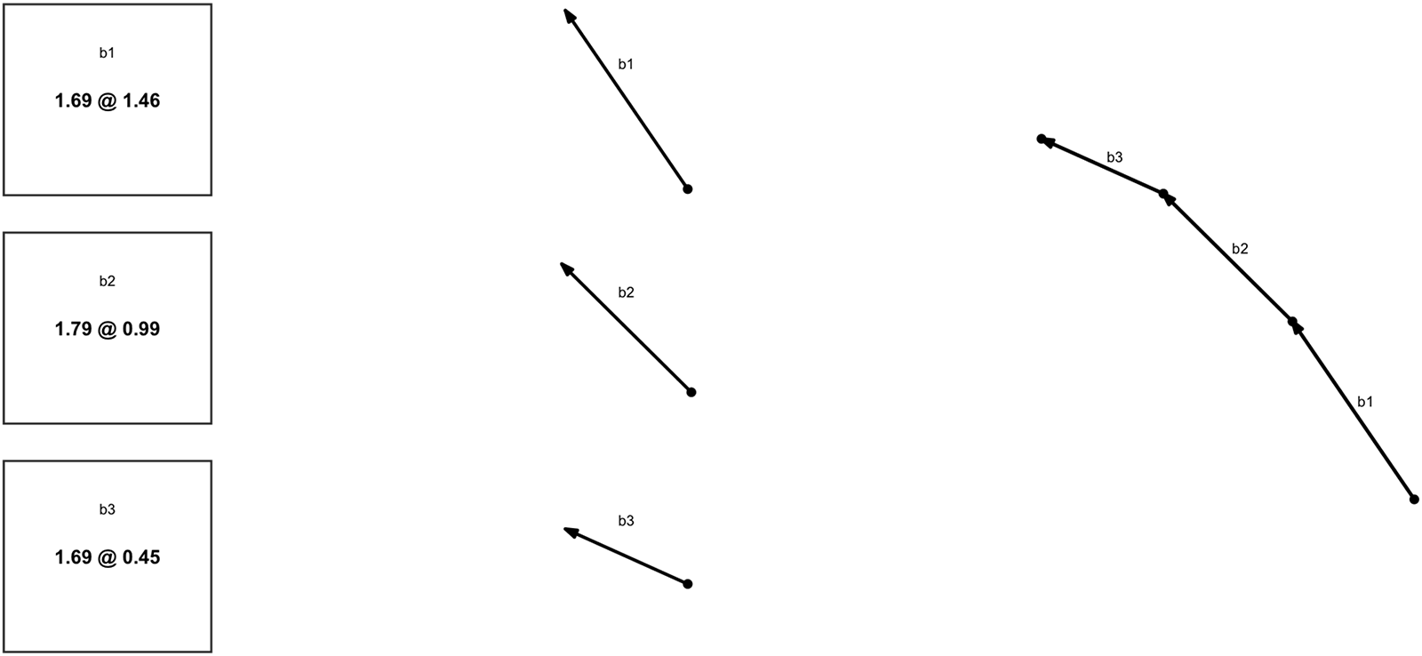
The other innovation, Frontier order book or FronOB, can be explained as a multi-step transformation of the order book display. The first column in Figure 6 shows the text bid queue from the left side (red box) in Figure 7, dropping the trader’s own bid because only other traders can accept it. The second column in Figure 6 draws each bid as a jump  $(\Delta x, \Delta y)$ from one allocation to another, that is, as an arrow of appropriate length with slope $p=\Delta y /\Delta x$. The third column places these arrows in order, tail-to-tip, starting with the best bid. Note that the slope (i.e., the bid price) decreases as we move down the order queue, so the resulting piecewise linear frontier is convex towards the origin. In an analogous fashion, the ask queue can be transformed into a convex piecewise linear frontier.
Transforming a bid queue. The first column repeats the text display, second column draws the corresponding vectors and third column shows the corresponding bid frontier

Combo User Interface. Left: full orderbook and trade history, price/quantity fields disabled for text entry. Right: Preference-inducing heatmap and order book frontier

The heatmap on right side of Figure 7 features the FronOB display constructed as just explained. The queue of bids by other traders in the box on the left transforms into the frontier (line segments connecting green dots; arrow heads suppressed) stretching Northwest from the current allocation (black dot). The queue of other traders’ asks transforms into the piecewise linear frontier (lines connecting red dots) stretching Southeast from the current allocation. Thus in Figure 7 the text order book transforms into a piecewise linear frontier through the current allocation. The CDA priority ordering by price (worse ask price  $ \gt $ best ask price $ \gt $ best bid price $ \gt $ worse bid price) ensures that this frontier is always convex.
FronOB allows the trader to see exactly what will happen with any click she chooses to make on the heatmap. The usual CDA rules imply that if she clicks inside the frontier then she will move exactly to the x-allocation in her click, and to the y-allocation on the frontier directly above her click (so she will have at least as much y as requested). If that point is above her indifference curve, then it will directly increase her utility and payoff. If she clicks above the frontier, her order will go straight into the order book, and will appear as a new line segment on other traders’ screens. On her own screen it appears as a pink dot if in the buy rectangle (to the Northwest of the current allocation), or as a pale green dot if in the sell rectangle.
Compared to the traditional implementation (TextOB), the innovation (FronOB) again would seem to reduce the trader’s cognitive load. The order book and order placement innovations are highly complementary — FronOB is much less useful if the heatmap is not clickable, and PnC-OP is especially useful when the presence of FronOB enables the trader to see exactly what will happen when she clicks.
3.3. GUI treatments
Table 2 lays out the features of the four user interfaces that our experiment compares. The first interface, called Texty and illustrated in Figure 4, is traditional. It has no heatmap, just the large payoff table, and has text order placement and text orderbook display. The interface called VideoGame, illustrated in Figure 8, is the polar opposite. It features a heatmap and the innovations heatmap enables, FronOB and PnC-OB, as the sole means of order placement and order book display.
VideoGame treatment User Interface. Left: visualized trade history using order lines (-slope = price, length = volume, and color = participation). Right: Preference-inducing HeatMap and Frontier OrderBook

User Interface Features. OB = Order Book; -OP = Order Placement. A ✓ in the column for a given interface indicates that the feature in that row is present

There is enough real estate on a trader’s screen to include both traditional and innovative displays, so we include a third interface, called Combo and illustrated in Figure 7, that does so. Our thought is that some traders might be more comfortable visualizing, and others might be more comfortable with traditional text, and Combo can accommodate both. Finally, to help separate the impact of the heatmap per se from the innovations it enables, we consider an interface called NoFrontier, illustrated in Figure 5. It is like Combo except that it suppresses FronOB and relies only on TextOB to display the orderbook.
Although this set of four treatments seems to include the most relevant feature combinations, its limitations should be acknowledged. A glance at Table 3 shows that our design conflates HeatMap with PnC-OP, and also conflates TextOB with Text-OP. There are natural complementarities within each conflated pair, but for the sake of completeness, followup research might explore other treatment combinations that disentangle their separate effects.Footnote 3
Summary of Experimental Sessions by Interface and Participant Experience. Each interface was tested in 4 sessions with inexperienced participants and 2 sessions with experienced participants. Each session consisted of two blocks, one using the HiPos and the other using the LoNeg parameterizations detailed in Table 1; the block sequence alternates across sessions

3.4. Other treatments
Our focus treatment variable is the user interface, with the four levels just explained. To promote robust inferences, the experiment includes two other “nuisance” variables. One of them is preference parameterization, with the two levels (HiPos and LoNeg) laid out in Table 1 and Figure 3 above. The other nuisance variable is experience level. Subjects in the Inexperienced treatment are first time participants from the LEEPS lab pool. Following tradition for complex market experiments, we ran additional sessions using participants from prior Inexperienced sessions. In recruiting for those Experienced sessions, we screen out participants whose earnings were in the bottom 30% in their Inexperienced session.
3.5. Implementation
The market platform customizes oTree (Chen et al., Reference Chen, Schonger and Wickens2016) software; it is posted at https://github.com/Leeps-Lab/otree_visual_markets. Each laboratory session lasts approximately 105 minutes. Participants are recruited through ORSEE (Greiner, Reference Greiner2015), and all sessions are conducted in person at the UCSC LEEPS Lab.
There are 24 sessions in total: 16 with inexperienced participants and 8 with experienced. Each session involves 10 traders per period (5 in the natural buyer role and 5 natural sellers)Footnote 4 and consists of two blocks with an equal number of consecutive periods with a role switch between blocks. The interface treatment varies across sessions, while the parametrization treatment varies within sessions: each block uses a different parameter set, and block order is reversed in even numbered sessions to control for potential order effects.
Inexperienced participants are all first-time subjects. Their sessions include instructions, videos, FAQs, a comprehension quiz, two practice periods, and twelve three-minute trading periods. They earn an average of $28.42, including an $8 show-up fee. Experienced participants (drawn from the top 70% of Inexperienced sessions) complete 18 trading periods (2.5 minutes each) with the same onboarding procedure. Their average payment is $30.58, including the show-up fee.
4. Results
To set the stage for formal comparisons of market outcomes across the different user interfaces, we begin with descriptive overviews of the data in Section 4.1. Estimates of treatment effects are reported in 4.2.
4.1. Descriptive statistics
Transaction Prices. Detailed raw transaction price data are graphed in Appendix Figures A.1.ab - A.2.ab. Here we consider the period-by-period average transaction prices  $\bar{p}_t$, computed as quantity-weighted averages within each period or, equivalently, as the total $y$ (numeraire) traded divided by the total $x$ traded in period $t$. Ideally, $\bar{p}_t $ approximates $ p_C$, at least in later periods.
Figure 9 shows  $\bar{p}_t$ averaged across all relevant sessions, with shading to indicate 95% confidence intervals. The price plots generally flatten and cling more closely to the CE price as more visual features are employed in the interface. Texty HiPos markets first under- and then over-price, and Texty LoNeg markets move away from CE in later periods even in experienced sessions. Average price converges to CE quite well in VideoGame markets regardless of experience level, especially with LoNeg parameters. Price convergence is less impressive but not bad overall in NoFrontier and Combo markets.
Average transaction price. Horizontal dotted (dashed) line is CE benchmark price for HiPos (LoNeg) parameters. Dots connected by lines show  $\bar{p}_t$ averaged across sessions; shaded area covers a 95% confidence interval. Separate panels show results for HiPos and LoNeg periods and for Texty, VideoGame, Combo and NoFrontier sessions. Upper panels: inexperienced traders. Lower panels: experienced traders

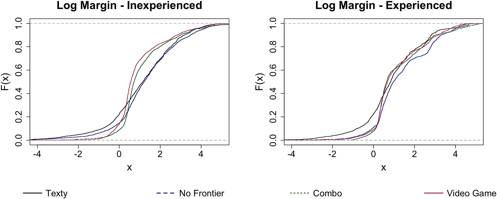
Figure 10 shows empirical cumulative distributions of the extent to which individual traders shade their transaction prices away from their personal marginal valuations. At each transaction, for the seller we record the proportional markup  $ln(p/MRS)$ of the transaction price $p$ over the marginal rate of substitution at her pre-trade MRS. For the buyer, we record the analogous personal markdown $ln(MRS/p)= -ln(p/MRS)$. The empirical distributions exhibit approximate second-order stochastic dominance (SOSD) orderings: as the UI becomes more visualized, margins (negative as well as positive) shrink. Negative values imply trading at a loss, and they are most common in Texty sessions, regardless of experience level. In inexperienced sessions, the presence of a frontier orderbook further reduces the number of negative trading margins, and also reduces the number of large positive margins. In experienced sessions, the distributions seem tighter overall, and tend to be tightest (e.g., the majority of proportional margins lie in the 0.2 - 0.9 range) in the formats (VideoGame and Combo) that include the frontier orderbook.
Margin cumulative distributions. Here  $x=(-1)^{I_{sell}}ln(MRS/p)$, where $I_{sell}$ is the indicator for the sell-side of a trade, MRS is the trader’s pre-trade marginal rate of substitution, and p is the trade price

Order placement channels. In the Texty (resp. VideoGame) treatment, traders must place their orders via Text-OP (resp. via PnC-OP), but in Combo and NoFrontier they can use choose either channel. Which do they prefer?
As explained in Appendix A, available data enable rough estimates. The basic idea comes from followers of Reinhard Selten such as Albers and Albers (Reference Albers and Albers1983): “prominent” prices (e.g., 2.50 but not 2.34) will be much more frequent when humans must choose prices and enter them manually than when they are computed from clicked pixels. Evidence suggests that about 16% of orders are placed using Text-OP in Inexperienced NoFrontier sessions. The Text-OP channel apparently is hardly ever used in Combo sessions and in Experienced NoFrontier sessions. Evidently the PnC-OP channel is strongly preferred when it is available.
Transaction size and trade volume. Appendix Tables A.2 - A.3 indicate that the size of individual trades  $(\Delta x)$ tends to be a bit smaller in early periods and on average is much smaller with Texty than with the other interfaces. Our interpretation is traders gain more confidence over time, and that PnC-OP is a major confidence booster.
The same tables show that trade volume starts out low in Texty sessions, but elsewhere is more than sufficient to reach allocations near competitive equilibrium. Whether traders actually achieve highly efficient final allocations (rather than trading to distant but inefficient points) is a different question to which we now turn.
Final Personal Prices. As noted in Section 2.2, efficiency can assessed in terms of the dispersion of personal marginal rates of substitution at the final allocation in each period. In CE, dispersion falls to zero from initial SLMRS levels of 2.28 in HiPos and 4.04 in LoNeg.
Figure 11 graphs the observed final MRS for individual traders and trader type averages. Again, markets seem more efficient as the interface becomes more visual, particularly in inexperienced sessions. Texty markets exhibit notable gaps from CE prices and, especially for LoNeg, non-convergence to any uniform value. These inefficiencies seem to shrink with each step downward in the panels. Convergence is especially impressive in all VideoGame markets and in experienced Combo markets.
Individual trader  $MRS_i$ at end-of-period allocations (dots) and type averages (lines); natural buyers (sellers) are red (green). Left: inexperienced traders. Right: experienced traders

Allocations. We now look more directly at final allocations within the Edgeworth box. Figure 12 plots aggregated Type A (natural buyers) vs B (natural sellers) final allocations in all periods. Those allocations in Inexperienced Texty sessions are erratic, and overtrading is not uncommon in HiPos blocks. In NoFrontier sessions, those allocations seem to spread out mainly along the path from initial allocation to (or even beyond) the CE allocation. Combo sessions have mostly near-Pareto efficient allocations, which spread out along the contract curve in inexperienced sessions but tighten up in experienced sessions. Finally, VideoGame aggregated final allocations are nearly Pareto optimal and bunch much tighter around the CE allocation. All of these trends are consistent across parametrization and across experience level, with the clusters tightening with experience.
Final allocations for aggregated agents at each periods. Light grey (or black) dots are for each period of inexperienced (or experienced) sessions. Red (or blue) diamond represents the CE (or initial) allocation

Payoff Efficiency. The first four rows of Table 4 report payoff efficiency ( $E_t$), realized gains as a fraction of CE gains, averaged over all periods in each treatment. Both parameterizations in the Inexperienced data exhibit a clear trend: $E_t$ increases as the UI becomes more visual, moving down the Table from one row to the next. The only exception is a minor decrease from 96 to 94% efficiency in HiPos efficiency as we move from Combo to VideoGame. Moving from Texty to VideoGame yields an increase in payoff efficiency of 16 to 28 percentage points. Trends are roughly similar but more compressed in experienced sessions, since efficiency there is generally higher, and Combo takes a slight lead as the most efficient interface.
Round Average Efficiency Metrics (and standard deviations). Payoff Eff. ( $E_t$), Price Eff. ( $P_t$) and MRS Eff. ( $M_t$) are defined respectively in equations (6),(5), and (3)

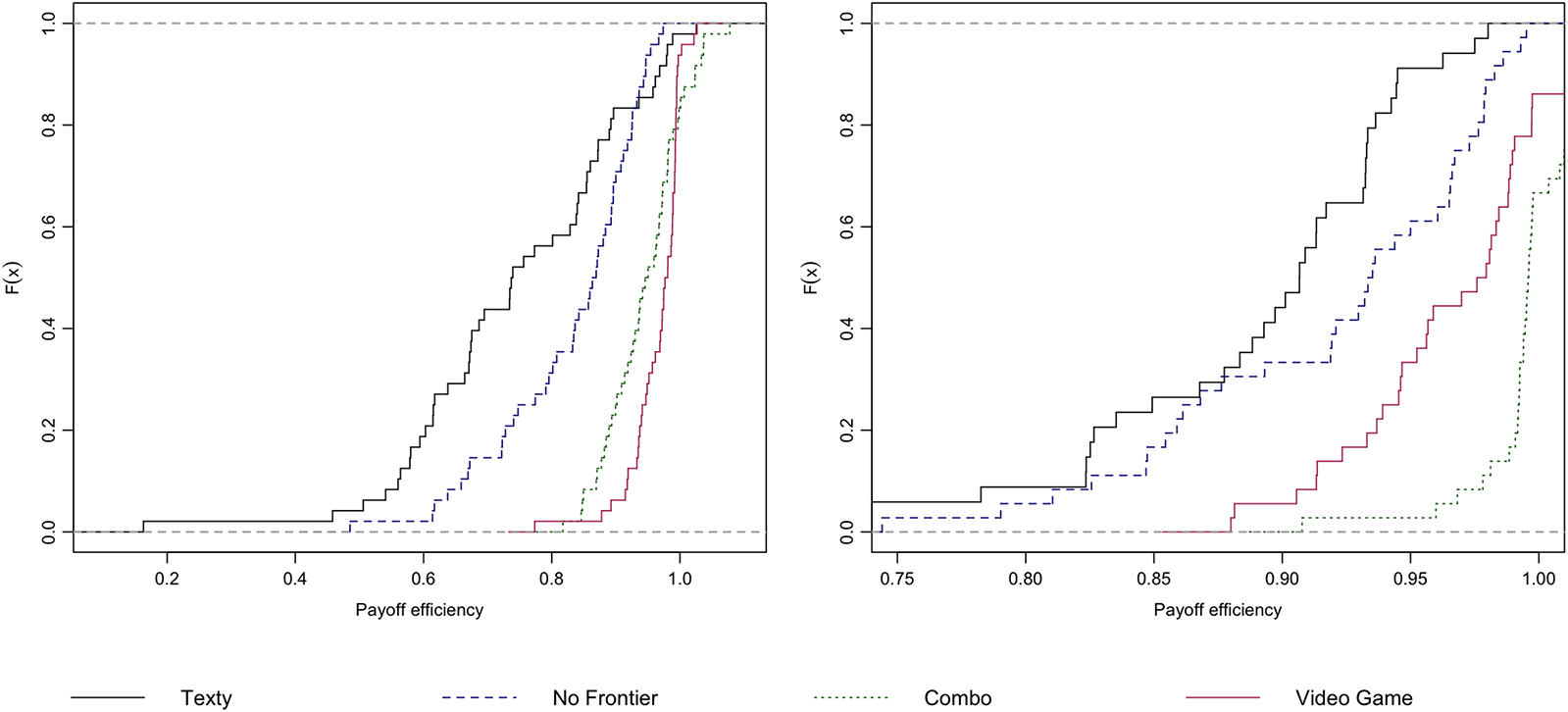
Fig. 13 offers a finer-grain comparison, using cumulative distribution functions of payoff efficiency values pooled across parametrizations. One sees almost first-order stochastic domination as one moves towards more visual interfaces with inexperienced subjects. The support of each distribution shrinks drastically (note the different horizontal scales!) when moving to experienced sessions; in Texty markets the smallest observations rise from below 0.2 to nearly 0.8. As suggested by the table, in experienced sessions Combo efficiency exceeds VideoGame, although both are quite high.
Cumulative distribution functions for payoff efficiency  $E_t$. Black, blue-dash, green-dot and red lines respectively indicate Texty, NoFrontier, Combo and VideoGame data. Left: inexperienced sessions. Right: experienced sessions

Fig. 14 looks at trends within period. At each second within a period, the payoff efficiency at the current allocation is averaged over all periods with the same parametrization, interface, and experience level; shaded bands indicate the 95 percent confidence interval across those periods. In inexperienced LoNeg sessions, there is clear separation that persists throughout the period from start to finish: efficiency rises fastest and remains highest with VideoGame, followed by Combo, followed by NoFrontier, with Texty lagging badly. The ordering is similar the other cases, with Combo catching up with VideoGame in Inexperienced HiPos sessions, and NoFrontier joining them in experienced LoNeg sessions. In every case, the payoff efficiency of Texty lags that of the more visual interfaces.
Within Period Average Payoff Efficiency by treatment. Black, blue, green and red lines (and shading) respectively indicate Texty, NoFrontier, Combo and VideoGame averages (and 95% confidence intervals). Left: Inexperienced. Right: Experienced. Top: LoNeg. Bottom: HiPos

Table 4 also reports the other two efficiency measures introduced in Section 2.3. The middle panel of the table reports price efficiency ( $P_t$), the relative deviation of the observed period-average price from the CE benchmark. Price efficiency again tends to increase as we add more visual features to the interface, regardless of experience. The exception: price efficiency in LoNeg Combo markets falls below that even in Texty markets. The reason can be seen in Figure 12, where Combo allocations in the wider lens fan out along the contract curve rather than clumping near the CE allocation. This underscores the point that the CE benchmark is only one of many Pareto optima in our economy, so price efficiency does not really capture actual vs potential gains from trade.
Our final efficiency measure aims to fill that gap. The bottom panel of the Table reports MRS efficiency ( $M_t$), the reduction in proportional dispersion among individual traders’ marginal rates of substitution at final allocations; it may be thought of as a price-space indicator of the potential gains from trade actually captured. In almost every case, we see MRS efficiency climb as we move downward in the table towards more visual interfaces, and across as we move from inexperienced to experienced traders. The only exception is that, with experienced traders, Combo reaches higher levels (a 93% reduction in proportional MRS dispersion) than in Videogame (still impressive reductions of 86-87%).
4.2. Treatment effects
To detect the impact of the user interface treatments, we run regressions of the form
 \begin{equation}
Y = \alpha + \sum_{i=1}^3 \beta_{i} \cdot {D_i} + \sum_{i=1}^3 \beta_{3+i} \cdot D_i \cdot \text{HiPos} + \beta_{7} \cdot \text{Period} +\epsilon
\end{equation}
\begin{equation}
Y = \alpha + \sum_{i=1}^3 \beta_{i} \cdot {D_i} + \sum_{i=1}^3 \beta_{3+i} \cdot D_i \cdot \text{HiPos} + \beta_{7} \cdot \text{Period} +\epsilon
\end{equation} The outcomes  $Y$ of interest include the three efficiency measures from Table 4: payoff efficiency, price efficiency and MRS efficiency. The key explanatory variables are indicators $D_i$ of UI treatments NoFrontier ( $i=1$), Combo (2) and VideoGame (3). The explanatory variables also include a period-level time trend and the parameter set indicator HiPos, along with its interactions with the UI treatments.
Table 5 reports OLS coefficient estimates for (7) separately for Inexperienced and Experienced data; as is now customary in market experiments, standard errors are clustered at the session level. Using (just before) the first period of LoNeg Texty as the baseline, the Table reports payoff efficiency gains ranging from 13 percentage points (borderline significant) for NoFrontier up to 27.5 pp (highly significant) for VideoGame in Inexperienced data. In Experienced data, the gains are generally smaller (presumably due to a higher baseline) but at least as significant, and perhaps even larger for Combo than for VideoGame. HiPos parameters raise the baseline 4-10pp but mostly shrink user interface treatment gains, likely due to the narrower lens of mutual gains in that parametrization.
Regressions on treatment identifiers. Standard errors (in parentheses) are clustered at the session level. Three observations are omitted from the Inexperienced MRS Eff calculation because they are at the boundary of allocation space where MRS is undefined

*, **, *** denote  $p \lt $0.1, 0.05, 0.01.
Table 5 reports similar gain patterns for MRS efficiency. When significant, price efficiency gains for the more visual treatments are always positive; their insignificance for Combo likely is due to the tendency discussed in the previous subsection for final allocations in this treatment to spread out along the contract curve. Appendix A.6 reports generally similar results for regressions that replace the time trend by period fixed effects and that replace the UI treatments by specific UI features. The general lesson seems to be that trade becomes more efficient when more of the visual features are available.
5. Conclusion
Our experiment can be summarized briefly. We explore territory of longstanding economic interest that previously seemed largely inaccessible to laboratory investigation: two-way trade of highly divisible goods with interdependent valuations. To access that general equilibrium (or Edgeworth box) territory we introduce novel graphical user interfaces (GUIs) that enable traders to visualize the interdependent valuations, to visualize the orderbook, and to use mouse point-and-clicks to propose and consummate trades.
We find that those videogame-like features generally speed up extraction of mutual gains from trade, and lead to more efficient final outcomes. For example, in our LoNeg economy, inexperienced traders using a traditional GUI took more than 5 times as long on average as those using our VideoGame GUI to extract half the potential gains from trade, and by the end of a trading period they were only able to extract on average about 70% of the potential gains versus over 95% for the VideoGame traders (see Figure 14, Panel A).
One practical question is whether a purely visual GUI (as exemplified in our VideoGame treatment) is better than a GUI which combines visual with traditional elements (as in our Combo treatment). For that question our results are mixed. With inexperienced traders, VideoGame had a consistent advantage, but with experienced traders Combo had a narrow lead in payoff efficiency (total gain extraction) and MRS efficiency (reducing dispersion in personal prices).
Such mixed results raise questions about which metrics are most useful for assessing market performance. It seems to us that MRS efficiency and payoff efficiency capture mainly the short term (within-period) dynamics of harvesting potential gains from trade, while price efficiency responds more to long term (across-period) dynamics that may push prices towards competitive equilibrium (CE). Some of our visual features seem better at encouraging moves towards the contract curve than specifically towards CE. But is that a bad thing?
Most importantly, our study opens new avenues for future research. Followup work with improved software could investigate the separate effects of features that are conflated in our present design, e.g., HeatMap and PnC-OP. A path is now open for investigating more interesting Edgeworth boxes than our HiPos and LoNeg, or for dealing with more than two interdependent goods. More broadly, we hope that our new interfaces will inspire new research into how visualizations and other cognitive aids can improve economic performance in other market or non-market contexts.
Supplementary material
The supplementary material for this article can be found at https://doi.org/10.1017/eec.2026.10043.
Replication package
The replication material for the study is available at https://doi.org/10.17605/OSF.IO/6MJ8S.
Acknowledgements
For helpful comments on earlier drafts, we are grateful to Elena Asparouhova, Sean Crockett, John Duffy, John Ledyard, Heinrich Nax, Luba Petersen, Jean Paul Rabanal, Maro $\check{s}$ Servátka, Daniel Woods and audiences at Macquarie University in March 2025, the Bay Area Behavioral and Experimental Economics Workshop in May 2025, and the Australia-New Zealand Workshop in Experimental Economics in August 2025. The final version owes much to the anonymous review team at this journal. The human subjects protocol, HS3566, was approved by the IRB of UCSC.


 Open access