


Impact Statement
Shock trains are systems of shock waves which form in supersonic internal flows. In particular, they are a feature of some high-speed propulsion systems (ramjets and scramjets) where they provide flow compression between the inlet and combustion chamber. A deeper understanding of the nature of shock trains is crucial to the advancement of supersonic and hypersonic propulsion. In this study, we examine the effect of spanwise confinement on shock trains by comparing finite and quasi-infinite span domains. The effect of the finite span (i.e. sidewalls) is significant. Firstly, a much longer shock train is formed which we argue is due to the three-dimensional component of the boundary layer confinement whereby a longer shock train is required to accommodate the higher overall momentum deficit. Secondly, the sidewalls cause the main separation bubbles to disappear which in turn results in lower flow deflection and thus weaker individual shocks.
1. Introduction
Shock trains are systems of coupled shock waves which occur in supersonic internal flows (Reference Gnani, Zare-Behtash and KontisGnani, Zare-Behtash, & Kontis, 2016). The most important instances of shock trains are found in ramjet and scramjet engines in the isolator section downstream of the compressor. A normal shock contained within a duct will bifurcate into multiple shocks when the Mach number, boundary layer thickness and back pressure are sufficiently high (Reference Matsuo, Miyazato and KimMatsuo, Miyazato, & Kim, 1999; Reference Om, Viegas and ChildsOm, Viegas, & Childs, 1985). The boundary layer separation and thickening through the first shock confines and reaccelerates the bulk flow downstream. Therefore, subsequent shocks are required in order to meet the imposed back pressure condition. The pressure of the bulk flow oscillates though successive shocks and expansions, whereas the pressure at the wall rises gradually towards the exit pressure. The subsonic layer increases in thickness along the shock train until the entire flow is decelerated from supersonic to subsonic.
There are a number of parameters which determine the composition and behaviour of a shock train. Principally, these are the free stream Mach number ( $M_1$), the back/inlet pressure ratio ( $p_b/p_1$) and the confinement ratio ( $\delta _{99}/h$, where $\delta _{99}$ is the $99\,\%$ boundary layer thickness and $h$ is the domain half-height). The effect of the boundary layer Reynolds number ( $Re_{\theta }$) is generally considered to be weak in comparison (Reference Morgan, Duraisamy and LeleMorgan, Duraisamy, & Lele, 2014; Reference Om and ChildsOm & Childs, 1985; Reference RousselRoussel, 2016). A free stream Mach number of 1.5 is the approximate lower threshold for shock train formation (Reference Matsuo, Miyazato and KimMatsuo et al., 1999). Shock trains are generally composed of normal shocks within the range $1.5 < M_1 < 2$ and oblique shocks for $M_1 \geq 2$ (Reference Carroll and DuttonCarroll & Dutton, 1990; Reference Hunt and GambaHunt & Gamba, 2018). Additionally, the Mach number is positively correlated with the spacing between shock waves (Reference Cox-Stouffer and HagenmaierCox-Stouffer & Hagenmaier, 2001; Reference Weiss, Grzona and OlivierWeiss, Grzona, & Olivier, 2010), which is a geometric effect of the shallower Mach waves. In general, the shock train length has a quadratic dependency on back pressure (Reference BilligBillig, 1993; Reference Klomparens, Driscoll and GambaKlomparens, Driscoll, & Gamba, 2015; Reference Waltrup and BilligWaltrup & Billig, 1973). On the other hand, the structure of the shock train is largely independent of the back pressure so that a change in back pressure merely shifts the shock train upstream or downstream, as shown in our previous simulations (Reference Gillespie and SandhamGillespie & Sandham, 2022).
The confinement ratio ( $\delta _{99}/h$) measures the relative thickness of the boundary layer compared with the half-height of the domain. It is this ratio which is particularly important, rather than the boundary layer thickness itself. Pioneering work on confinement effects were carried out by Carroll & Dutton (Reference Carroll and DuttonCarroll & Dutton, 1988, Reference Carroll and Dutton1990, Reference Carroll and Dutton1992; Reference Carroll, Lopez-Fernandez and DuttonCarroll, Lopez-Fernandez, & Dutton, 1993) who used experimental and computational results to show how more highly confined shock trains were composed of a higher number of weaker shocks. Similar results were found by Reference Geerts and YuGeerts and Yu (2015) who increased the confinement ratio by reducing the domain height while maintaining the same boundary layer, which resulted in the shock train leading edge being displaced upstream. The shock train length is generally considered to scale with the square root of the confinement ratio (Reference BilligBillig, 1993; Reference Waltrup and BilligWaltrup & Billig, 1973).
A less well understood factor affecting the behaviour of shock trains is the presence of sidewalls. Besides the additional confinement of the duct, other influences of the sidewalls such as secondary flows, corner and sidewall separations may be important. In incident-reflected shock-boundary-layer interactions (SBLI) arrangements, these additional phenomena are thought to have a strong effect on the bulk flow near the centreline, especially in the case of highly confined ducts (Reference Geerts and YuGeerts & Yu, 2016a). A consistent finding on the effects of sidewall confinement is that the shock structure and general flow arrangement is highly three-dimensional (3-D), even for large aspect ratio ducts (Reference Geerts and YuGeerts & Yu, 2016b).
Shock trains have also been studied using the Reynolds-averaged Navier–Stokes (RANS) approach. Reference Cox-Stouffer and HagenmaierCox-Stouffer and Hagenmaier (2001) systematically varied the Mach number and aspect ratio ( $W/H$, where $W$ is the duct width and $H=2h$ is the duct height). For the highest Mach number ( $M_1=3.2$) they found that increasing the aspect ratio (by widening the duct) was associated with shock train systems which were longer and settle farther upstream. For the lower Mach number ( $M_1=2.0$), however, the effect was more complicated, with the lowest aspect ratio square duct case settling furthest upstream. Additionally, it was noted that the quasi-two-dimensional (quasi-2-D) arrangement was, by its nature, lacking several key flow features associated with the sidewalls (corner separation, sidewall shocks, etc.). Reference Cox-Stouffer and HagenmaierCox-Stouffer and Hagenmaier (2001) suggest that a very large aspect ratio (much larger than their highest aspect ratio of nine) would be required for the effects of the sidewalls to become negligible.
The sidewall influence has been studied more recently by Reference Morgan, Duraisamy and LeleMorgan et al. (2014) where shock trains were analysed with both span-periodic conditions and sidewalls. By comparing the results with wind tunnel measurements, the sidewall case was found to match more closely to the experiments than the span-periodic case. Specifically, the span-periodic case underestimated the boundary layer growth rate, thereby predicting a lower level of confinement and producing a shorter shock train, even with a larger back pressure applied. Additionally, it was shown that the corner vortices present with the application of sidewalls (referred to as secondary flow) were able to extend beyond the boundary layer edge, and thereby influence the core flow. Another study by Reference Gnani, Zare-Behtash, White and KontisGnani, Zare-Behtash, White, and Kontis (2018) confirms the differences between 2-D/quasi-2-D and fully 3-D arrangements, with the 3-D case exhibiting larger pressure increases/decreases through the centreline of the shock train. The inaccuracies compound over the subsequent shocks, leading to the 2-D case overestimating the downstream Mach number and slightly underestimating the exit pressure.
It has been suggested by Reference Vane and LeleVane and Lele (2013) that the difference between cases with and without sidewalls can be explained by the overall blockage of the cross-section. By doubling the height of the boundary layer of a span-periodic case (thereby approximating the overall blockage with sidewalls) they found good agreement with wind tunnel measurements. This finding would imply that, at least in some configurations, the corner flow plays a much lesser role in the shock train behaviour compared with the additional displacement effect of the sidewall boundary layers.
In the current work we use scale-resolving numerical simulations to study the effect of sidewalls on the structure and composition of shock trains. In the following section the methodology for the simulation is outlined and the results of the grid refinement study are presented. In § 3 we explore the sidewall effects on the turbulent boundary layer without the presence of the shock train. The main focus of the paper is given in § 4 where we discuss the effect of the sidewalls on the overall flow field (4.1), shock pressure distribution (4.2) and shock structure (4.3).
By comparing two domains of finite and infinite span we find that the sidewalls significantly lengthen the shock train, which we suggest is an effect of the larger overall boundary layer momentum deficit. A modification is made to a commonly used shock train scaling model, where we find an improved collapse of the pressure distributions of the two cases at the tested conditions. Additionally, we find that the sidewall case exhibits lower shock pressures and lower wall-normal velocities, likely due to the lack of a large separation region at the shock train leading edge.
2. Numerical methods
2.1 Methodology
The simulations presented here were performed using a direct implementation of the full Navier–Stokes equations. The formulation is described below in tensor (Einstein) notation. Firstly, the conservation of mass, momentum and energy
 \begin{gather} \frac{\partial \rho}{\partial t} + \frac{\partial \rho u_j}{\partial x_j} = 0, \end{gather}
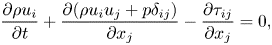 \begin{gather}\frac{\partial \rho u_i}{\partial t} + \frac{\partial (\rho u_i u_j + p \delta_{ij})}{\partial x_j} - \frac{\partial \tau_{ij}}{\partial x_j} = 0, \end{gather}
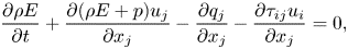 \begin{gather}\frac{\partial \rho E}{\partial t} + \frac{\partial (\rho E + p) u_j}{\partial x_j} - \frac{\partial q_j}{\partial x_j} - \frac{\partial \tau_{ij}u_i}{\partial x_j} = 0, \end{gather}
where  $\rho$, $T$,
$T$,  $E$ and $u_i$ are density, temperature, energy and velocity, respectively. Next, the pressure ( $p$), the viscous stress tensor ( $\tau _{ij}$), heat flux ( $q_i$) and dynamic viscosity ( $\mu$) terms are given by
 $$\begin{gather} p = (\gamma - 1)\left(\rho E - \frac{1}{2}\rho u_j u_j\right), \end{gather}$$
 $$\begin{gather}\tau_{ij} = \frac{\mu}{Re} \left(\frac{\partial u_i}{\partial x_j} + \frac{\partial u_j}{\partial x_i} - \frac{2}{3}\delta_{ij}\frac{\partial u_k}{\partial x_k} \right), \end{gather}$$
 $$\begin{gather}q_j = \frac{\partial T}{\partial x_j} \left(\frac{\mu}{(\gamma - 1)M_1^2Pr Re} \right), \end{gather}$$
 $$\begin{gather}\mu = T^{3/2} \frac{1 + T^ * _s/T^ * _1}{T + T^ * _s/T^ * _1}, \end{gather}$$
where  $Re$,
$Re$,  $Pr$,
$Pr$,  $M_1$ and $\gamma$ are the Reynolds number, Prandtl number, free stream inflow Mach number and heat capacity ratio, respectively. Here $T^*_s=110.4K$ is the Sutherland temperature (with the superscript $^*$ indicating a dimensional quantity) and $T^*_{1}=288.0K$ is the reference temperature. Other than these reference temperatures, the equations are dimensionless. Velocity, density, temperature and viscosity are normalised by the free stream quantities at the inflow ( $u_{1}$, $\rho _{1}$, $T_{1}$), with pressure normalised by $\rho _{1} u_{1}^2$. All lengths and coordinate values are normalised by the displacement thickness of the van Driest-transformed inflow boundary layer profile, $\delta ^*_{vd}$. All of the simulations model air as an ideal gas with $\gamma = 1.4$ and $Pr = 0.72$.
The solver used in the current work is OpenSBLI which is an explicit, finite difference code designed for shock wave/boundary layer interactions (Reference Jacobs, Jammy and SandhamJacobs, Jammy, & Sandham, 2017; Reference Lusher, Jammy and SandhamLusher, Jammy, & Sandham, 2018, Reference Lusher, Jammy and Sandham2021). Shock capturing is applied to the Euler terms of the simulations with a sixth-order targeted essentially non-oscillatory (TENO) scheme (Reference Fu, Hu and AdamsFu, Hu, & Adams, 2016). This scheme has been shown to demonstrate good stability for shock wave problems while still having a low enough dissipation to accurately resolve turbulence (Reference Gillespie and SandhamGillespie & Sandham, 2022). A fourth-order central scheme is used for the heat flux and stress terms and the time advancement is performed with a low-storage third-order Runge–Kutta (RK3) scheme (Reference Kennedy and CarpenterKennedy & Carpenter, 1994).
An outline of the general flow configuration can be seen in figure 1. In order to assess the effect of the sidewalls, two cases are considered in the current work. The channel case has solid boundaries on the top and bottom and is periodic in the spanwise direction while the square duct case is bounded on all four sides with solid walls. The inlet flow enters the domain at  $M_1=2$ with turbulent boundary layers forming on the solid walls. No-slip isothermal wall boundary conditions with wall temperature $T_w/T_1=1.676$ are applied to all solid surfaces. For the channel arrangement, periodic conditions are applied in the $z$ direction which mimics an infinite-span condition. The boundary layer turbulence is generated using a synthetic turbulence generation method at the inflow plane. The particular implementation is a modified version of the method outlined in Reference Kim, Xie and CastroKim, Xie, and Castro (2011) and Reference KimKim (2013) where length scales are applied to random disturbances which are then carried downstream, developing into realistic turbulent structures. At the end of the boundary layer development region at $x = 6h$ the key boundary layer properties (skin friction, turbulence intensity, correlation lengths) are sufficiently converged (see § 3). The spanwise integral length scales are of the order $0.1h$ meaning that the domain is considered wide enough to avoid any synthetic windowing effects when implementing the periodic boundary condition (see pp. 56–57 in Reference GillespieGillespie (2021)). Within the sponge zone a body-force term is applied to gently force the flow within the region to the target back pressure condition, $p_b$. The implementation of the sponge zone takes the form
 \begin{equation} p_n(x) = p_{n-1}(x) + (p_b - p_{n-1}(x))w(x), \end{equation}
where  $p_n(x)$ is the streamwise distribution of pressure at time step $n$ and $w(x)$ is spatially varied weight term. The sponge zone is only applied to the shock train cases where the condition $p_b/p_1 = 3.0$ is set. Additional information and validation of the sponge zone and turbulence generation can be found in chapters 3 and 4 of Reference GillespieGillespie (2021).
General outline of the shock train problem (channel case). The shock waves are shown by black lines and the circulating arrows by the leading shock represent the separation regions. The hatched area at the end of the domain represents the sponge zone.
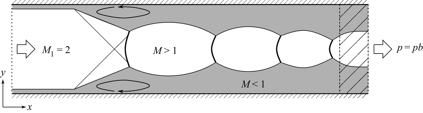
The channel has cross-sectional dimensions  $(l_y,l_z) = (2h,h)$ and the duct $(l_y,l_z) = (2h,2h)$, where $h$ is the channel half-height. The short and long domain cases are, respectively, $l_x=16h$ and $l_x=24h$ long. A streamwise distance of $6h$ downstream of the inflow is required for the turbulent boundary layer to develop, while the sponge zone occupies $2h$ from the outlet plane. The boundary layer properties at the inlet are $\delta _{99}/h=0.28$ and $Re_{\theta } = 500$, where $\theta$ is the momentum thickness. Details of the flow parameters at the inlet (station 1) and just upstream of the shock train (station 2) are given in table 1.
Summary of flow parameters at the inlet and shock train leading edge.

With long run times required for shock trains to develop, the Reynolds number of the current work is chosen to reduce the computational cost. At the domain inflow the conditions are  $Re_{\theta } = 500$ and $Re_{\tau } = 130$ which rise to 740 and 170 just at the leading edge of the shock train. These values are lower than most published large-eddy simulation (LES) and direct numerical simulation (DNS) results, which are themselves typically much lower than comparable wind tunnel results. For example, the minimum $Re_{\theta }$ values reported in Reference Morgan, Duraisamy and LeleMorgan et al. (2014) and Reference Fiévet, Koo, Raman and AuslenderFiévet, Koo, Raman, and Auslender (2017) are, respectively, 1660 and 4350 (although in the latter case the viscosity had to be multiplied by a factor of four to make the simulation more tractable). However, the Reynolds number is generally found to have a small effect on the structure of the shock train and a sensitivity study using the current methodology showed only a 12 % increase in the shock train length and an 8 % increase in shock spacing with a factor of two increase in Reynolds number (Reference GillespieGillespie, 2021).
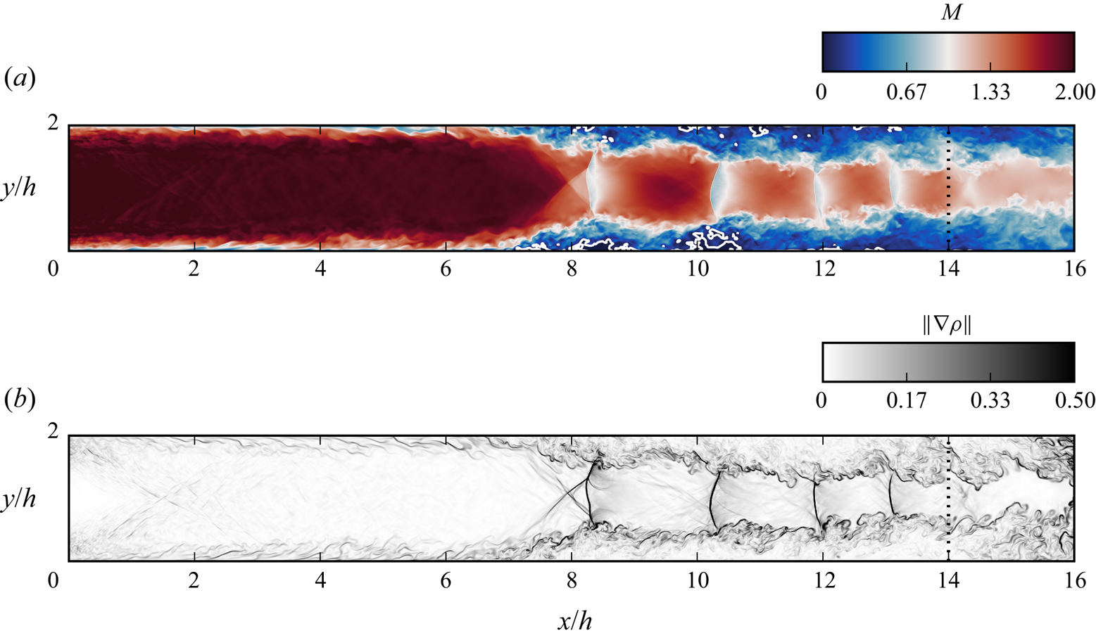
An example of a typical flow field for the channel case is shown in figure 2. Here we see images of Mach number and density gradient showing the position of the shock train within the domain. The shock train is composed of four shocks occupying roughly half the domain and each shock has a small pocket of subsonic flow immediately downstream. All of the shocks are normal other than the leading shock which has both normal and oblique components. The subsonic portion of the boundary layer thickens considerably through the shock train but there remains a supersonic region of the bulk flow up to the outlet plane. There is a significant boundary layer separation at the leading shock (approximately  $2h$ in length) as well as transient separations at the downstream shocks.
Instantaneous flow contours of Mach number (a) and density gradient (b) for the channel case. The edge of the sponge zone is indicated by the dotted black line. For the Mach number plot, isolines of  $M=0$ (separation) are drawn in white.
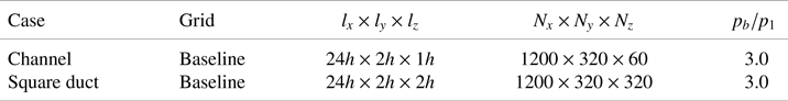
2.2 Grid refinement study
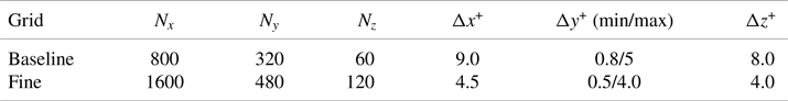
A grid refinement study was carried out in order to understand the sensitivity of the shock train flow properties to the mesh spacing. Here we compare two grid resolutions (denoted ‘baseline’ and ‘fine’), with details listed in table 2. The fine grid has twice the resolution in the streamwise and spanwise directions and  $50\,\%$ more in the wall-normal resolution. The reported viscous grid spacing values correspond to boundary layer conditions at $x=6h$ and, were it not for the need to capture shock waves and shock-induced separation, both grids would be considered as satisfying the usual conditions for DNS. All grid cases are run at the stated flow conditions in the previous section and use the shorter $l_x=16h$ configuration. Full details of the grid sensitivity of the turbulent boundary layer properties can be found in the supplementary material.
Summary of grid resolutions upstream of the shock train ( $x=6h$).
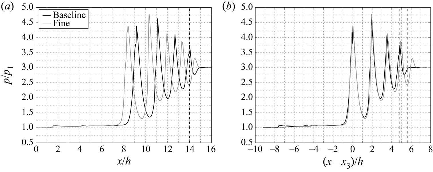
In figure 3 we plot two comparisons of centreline static pressure. First, no corrections are applied showing that the equilibrium position of the leading shock is particularly sensitive to the degree of grid refinement, with the shock train in the finer grid case sitting farther upstream. In figure 3(b) we account for this by aligning the distributions by the leading shock location ( $x_3$). Here, the two sets of curves collapse well, up to the fourth shock cycle. This suggests that the baseline grid is able to reliably predict the effects of the boundary layers on the shock train structure, including the strength and spacing of the shock waves and this grid is employed for the remaining cases discussed in the current work.
Grid sensitivity of the centreline static pressure distribution (a) without corrections and (b) corrected to match the leading shock location. Aligning the leading shocks allows the profiles to collapse together very well.
3. Turbulent boundary layer analysis
In this section we will consider the effect of sidewalls on the boundary layer development without the inclusion of a shock train. Two cases are compared, one channel and one duct, with no applied back pressure. While the channel case uses only the shorter configuration, the duct case was run with a longer ( $l_x = 24h$) domain in order to explore the development of the secondary flow vortices. Starting from a zero-disturbance boundary layer profile as the initial state, a period of $128h/u_1$ is allowed for the turbulent statistics to fully develop. After this, the statistics are captured over a period of 64 and $96h/u_1$ for the channel and duct cases, respectively. The span averaging of the duct case was conducted over the central $50\,\%$ of the domain.
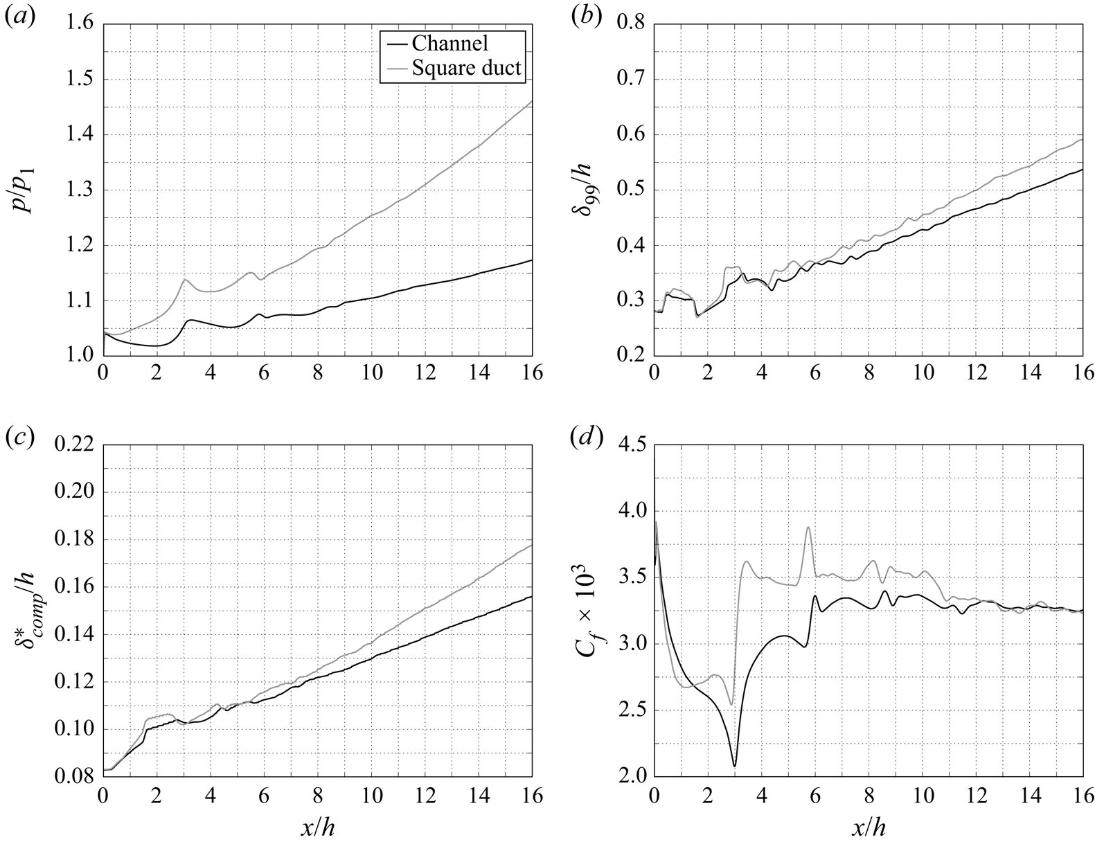
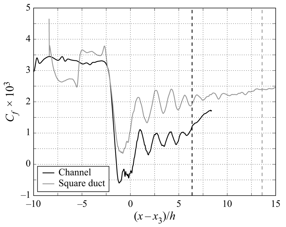
Plots of the streamwise flow properties (up to  $x = 16h$) are given in figure 4. Due to the presence of boundary layers on the sidewalls, the duct case incurs a larger degree of boundary layer confinement. Thus, the pressure increase in the duct case is significantly higher than the channel case and the difference becomes more pronounced farther downstream. One effect of this higher adverse pressure gradient is to increase the rate of boundary layer growth, both in the 99 % thickness and the displacement thickness. The skin friction distribution given in figure 4(d) shows that the sidewall confinement also raises the skin friction until approximately $x=13h$, after which there is good agreement between the two cases. An interesting feature of the duct case is that this is only a quasisteady state and after another ${\sim }100h/u_1$ time units a shock train forms naturally, even without the imposition of a specific back pressure.
Streamwise distribution of (a) wall static pressure, (b) 99 %  $u_e$ boundary layer thickness, (c) displacement thickness and (d) skin friction coefficient showing the effect of sidewalls on the enclosed boundary layer. The results of the duct case represent the quasisteady state prior to the natural formation of a shock train.
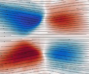
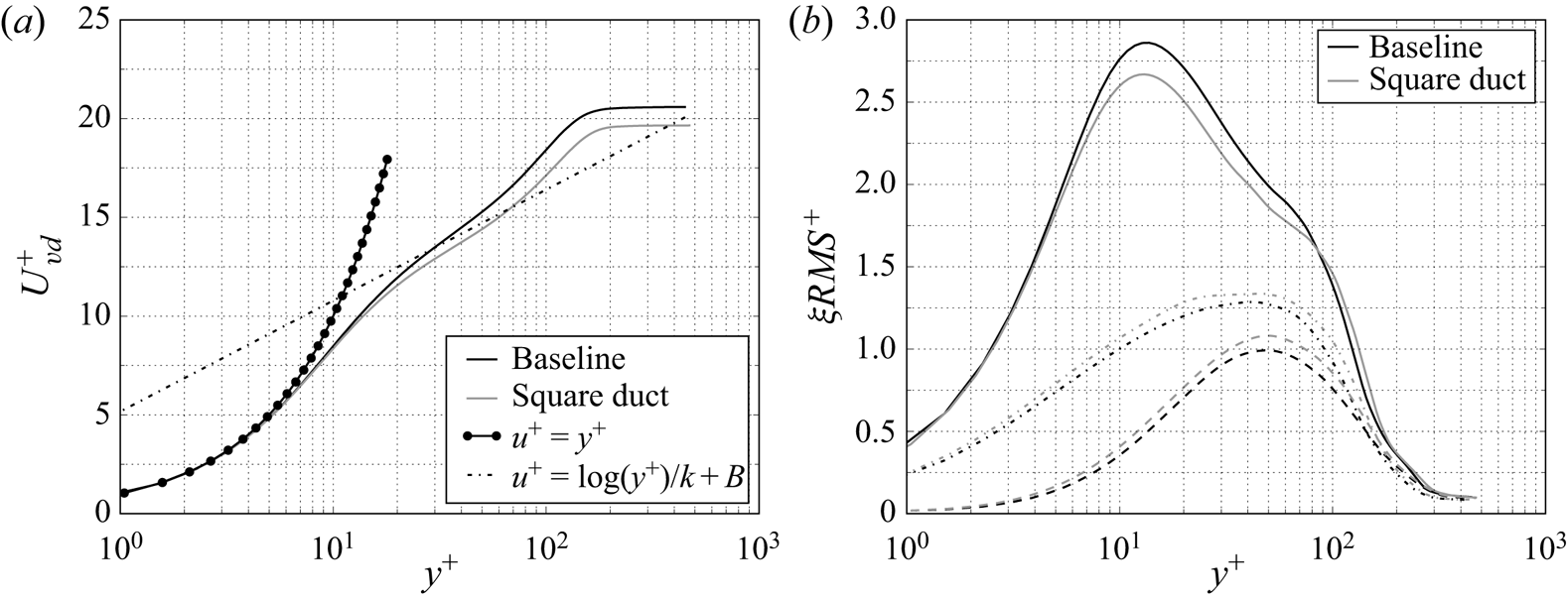
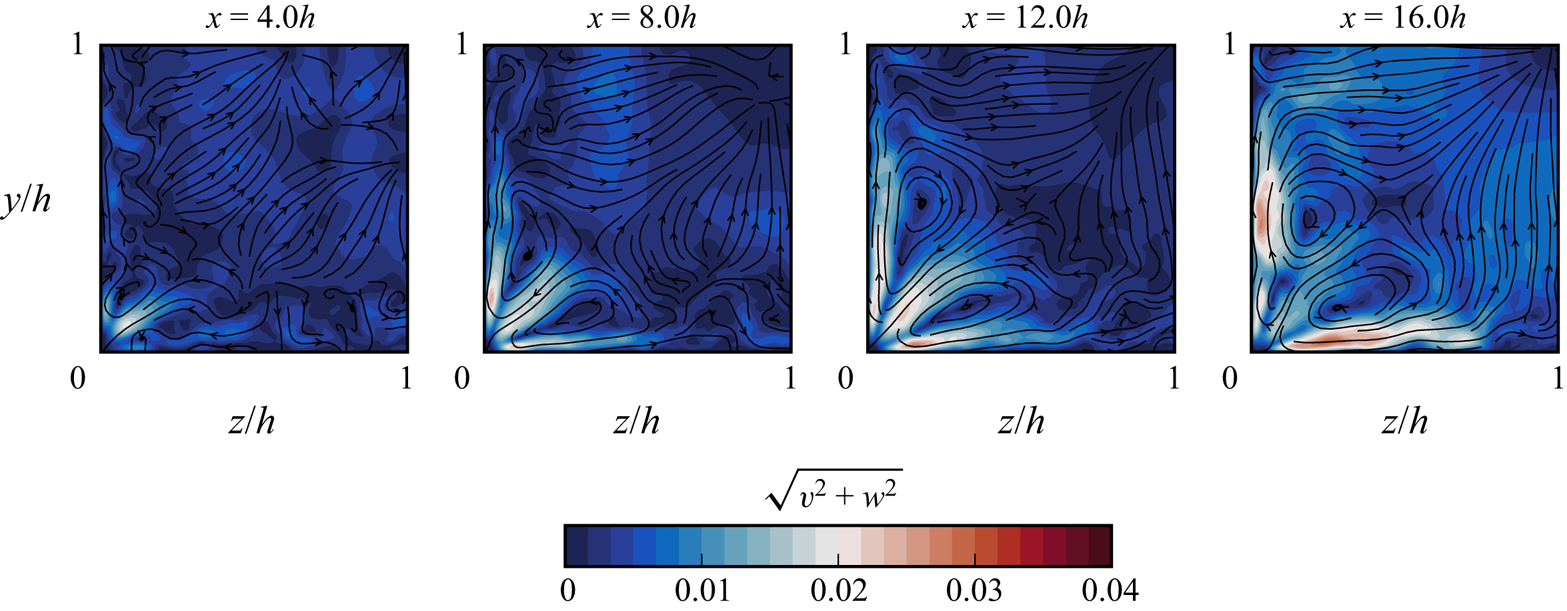
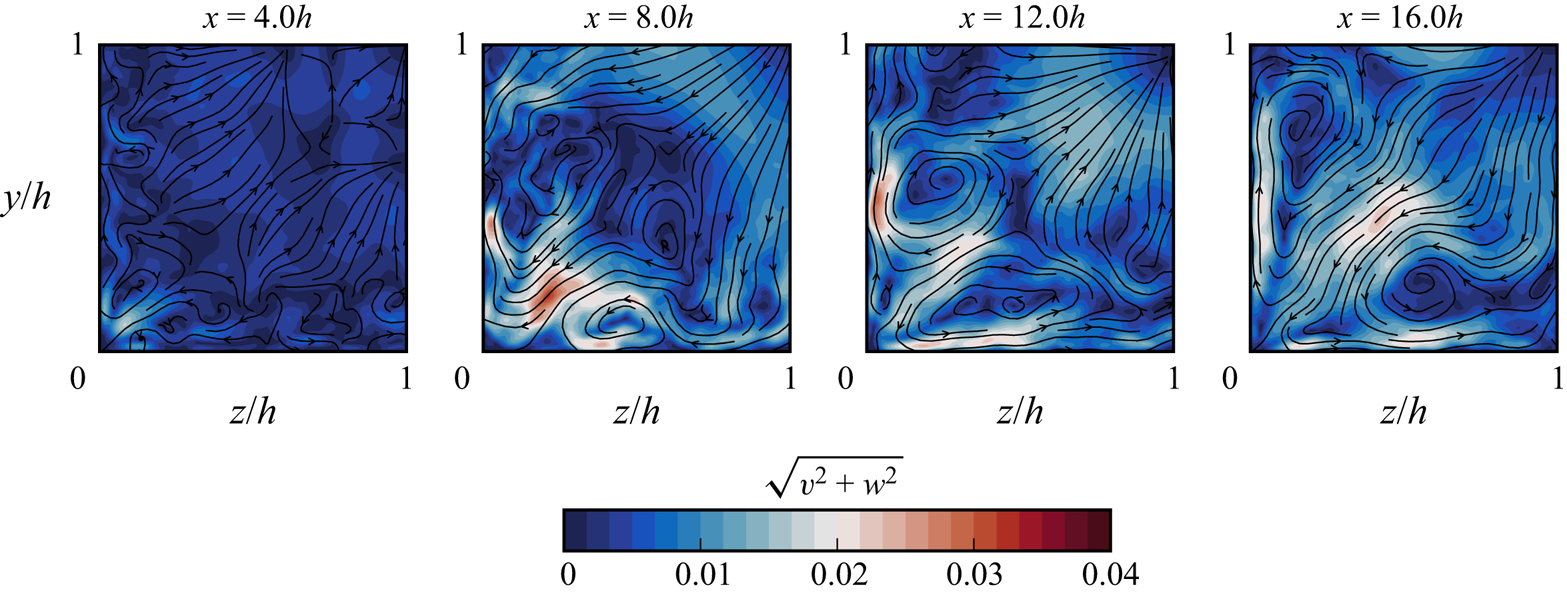
The sidewalls have a very limited effect on the boundary layer turbulence outside of the corner regions. This is illustrated in figure 5 where we plot van Driest transformed velocity and density-scaled Reynolds stress profiles at  $x = 8h$. Relative to the channel, the duct velocity profiles are displaced downwards towards the logarithmic law of the wall, the streamwise fluctuations are lower and the normal and spanwise fluctuations are higher. Secondary flow structures of Prandtl's second type have been previously identified in a variety of ducted flows, including in the supersonic regime (see for example Reference MorganMorgan (2012) and Reference Wang, Sandham, Hu and LiuWang, Sandham, Hu, and Liu (2015)). Such structures are also present in the current work as shown in figure 6. Here, streamlines of transverse flow velocity ( $v$,
$v$,  $w$) are plotted over a quarter of the duct cross-section at four streamwise locations. In each corner of the duct a vortex pair is formed, symmetrical about the corner bisector. The peak (time-averaged) velocity in each vortex reaches 2 % of the free stream velocity as flow is drawn towards and then away from the corner. There is incipient secondary flow at the $x=4h$ position and a complete vortex structure by $x=8h$. From there the vortices continue to grow in size as the boundary layers grow, until they occupy the entire cross-section of the domain. At this point the vortices are constrained by those in opposing corners and so remain at a constant size.
Boundary layer profiles of (a) van Driest-transformed velocity profile and (b) density-weighted Reynolds stress profiles (solid, dashed and dotted lines are RMS of  $u'$,
$u'$,  $v'$ and $w'$, respectively). All profiles are taken at $x = 8h$.
Velocity streamlines showing the emergence and development of secondary flow structures. Plots are coloured by transverse velocity magnitude,  $\sqrt {v^2 + w^2}$.
4. Shock train analysis
4.1 Finite and infinite span comparison
In this main section we discuss the impact of spanwise confinement on the shock train, comparing the results of channel and square duct cases. Both cases have the same domain length ( $l_x=24h$), back pressure ( $p_b/p_1 = 3.0$) and grid resolution (the baseline grid). A summary of each case is given in table 3.
Summary of shock train cases in the spanwise confinement study.
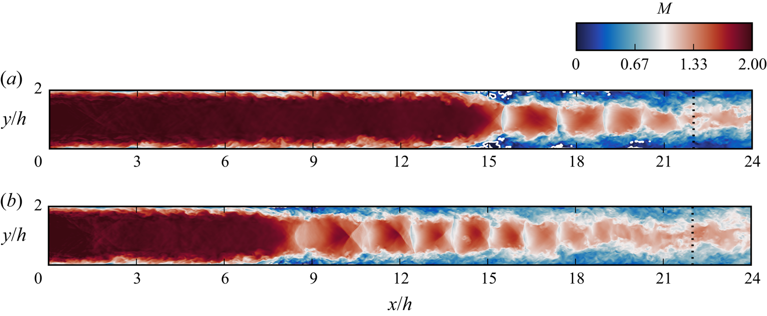
From an examination of the resulting flow fields it is immediately clear that the sidewalls have the effect of producing a significantly longer shock train. Figure 7 compares the Mach number at the midspan location of each case. In addition to a longer shock train and higher number of shocks, the structure of the shocks is also considerably different. The first two shocks in the square duct are weaker oblique structures and it is only until the third shock at  $x = 12h$ that there is subsonic flow at the centreline. As discussed in § 3, the sidewalls introduce a higher degree of boundary layer confinement and this has the effect of reducing the exit Mach number at the centreline.
Instantaneous flow contours of Mach number comparing the channel (a) and square duct (b) cases. The edge of the sponge zone is indicated by the dashed black line. For the Mach number plot, isolines of  $M=0$ (separation) are drawn in white.
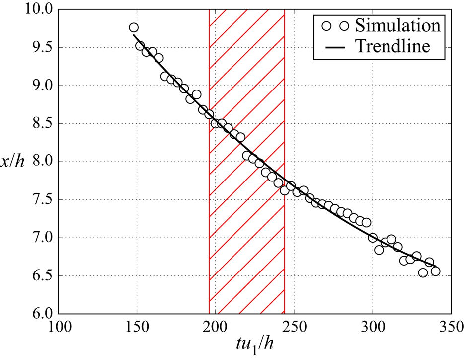
While the channel case produces a stable shock train within the region after the turbulent boundary layer has fully formed, the leading shock of the duct case eventually stabilises within the boundary layer development region. In order to avoid encroaching on this part of the domain, the data is captured while the shock train is slowly moving upstream (at around 0.75 % of the free stream velocity) in the region where the leading edge of the shock train interacts with a fully developed turbulent boundary layer. The time history of the leading shock location is shown in figure 8. Statistical data is captured for a period of  $48h/u_1$ as indicated by the red shaded area. Firstly we use a simple (termed ‘static’) average over this region and later we will use averages (termed as ‘dynamic’) in the reference frame of the shock train. The data capture period for the channel case is
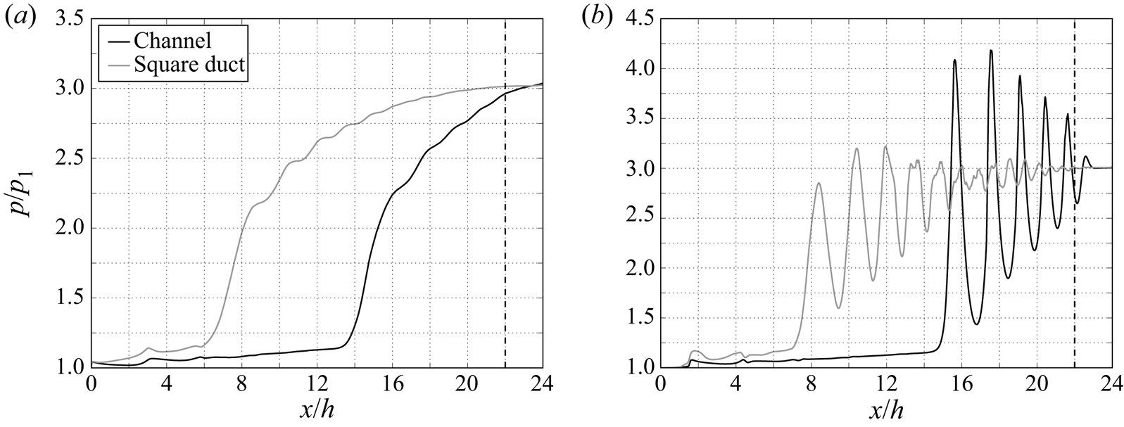
  $96h/u_1$ and occurs once the shock train has stabilised. Streamwise plots of wall pressure and centreline pressure are shown in figure 9. The data confirms the findings from the instantaneous flow pictures, namely, that the effect of the sidewall is to displace the shock train upstream. The furthest upstream instance of the duct case shock train occurs at around $x=6h$ which is at the established limit of the boundary layer development region. This is a similar problem to that encountered by Reference Fiévet, Koo, Raman and AuslenderFiévet et al. (2017) for their high grid resolution cases. In their case the preferred solution was to reduce the sampling time for the statistics.
Space–time plot of the leading shock position of the square duct case. The black curve is a second-order polynomial fit. The red hatched area indicates the period of data capture.
Sidewall comparison of streamwise distributions of pressure (a) at the wall and (b) at the centreline. The sidewalls cause a much longer shock train to form and the strength of the individual shock waves to be significantly weaker.
In figure 10 the streamwise pressure distributions have been aligned to match at the leading shock in order to more clearly compare the shock trains in the duct and channel cases. Additionally, the dynamic averaging method is used here for the duct case, in which the slow drift of the shock train is taken into account by assuming a time-varying  $x_3$ value and taking an average of $p(x - x_3(t))$. With regards to the wall pressure (figure 10a), the two case are well matched in the earlier portion of the shock train (between $(x-x_3)/h = -5$ and 0) which is a common result in SBLI and shock train problems (for examples see Reference Matheis and HickelMatheis and Hickel (2015) and Reference Gillespie and SandhamGillespie and Sandham (2022), respectively). Farther downstream of this the wall profiles diverge, with the duct case experiencing a lower pressure gradient through the remainder of the shock train. The two averaging methods are also compared here and it is clear that the effect on wall pressure is small. Also included in figure 10(a) is the wall pressure results from case B from Reference Fiévet, Koo, Raman and AuslenderFiévet et al. (2017) which is a finite span arrangement with the same Mach number and similar back pressure and confinement to the current work. The data from this DNS study agrees well with the results from the duct, although it is worth noting that the pressure distribution is somewhat flatter, likely due to the higher Reynolds number employed by Reference Fiévet, Koo, Raman and AuslenderFiévet et al. (2017).
Adjusted pressure distributions (a) at the wall and (b) at the centreline. The adjustment is made by aligning the leading shocks. The dynamic averaging method accounts for the movement of the shock train whereas the static averaging method does not.
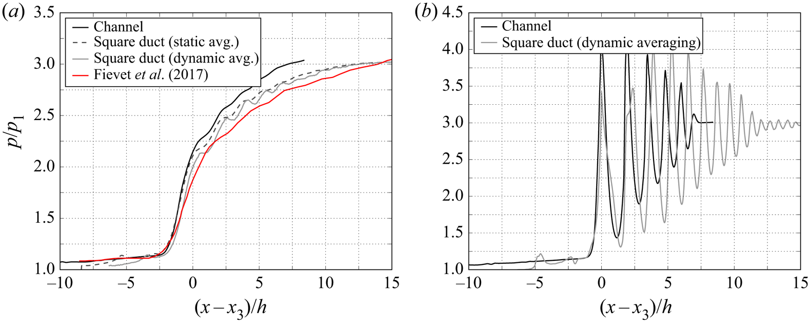
In terms of the centreline pressure, the differences between the channel and duct cases are considerable. The channel case has higher peak pressures at the first two shocks whereas the duct case has higher pressure after the third shock. Additionally, the shock spacing of the duct case is significantly larger. For clarity, the static averaging method line is omitted from figure 10(b) since it is clear, by comparing with figure 9(b), that the movement of the shock train should be accounted for in this case.
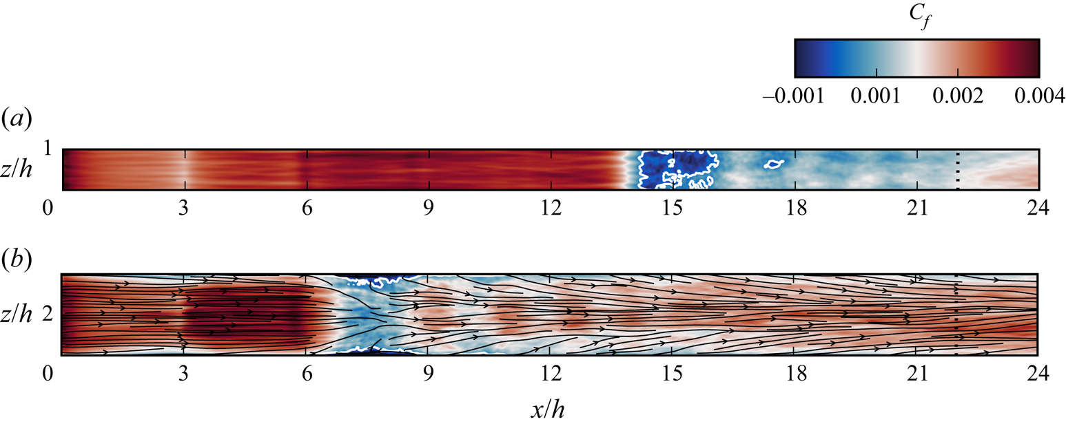
Figure 11 shows a comparison of time-averaged skin friction over the bottom wall. The reverse flow regions (associated with  $C_f < 0$) are shown in dark blue and bounded by white lines. While the channel case has a very large separation bubble (covering the whole width of the domain) at the head of the shock train, the separation in the duct case only exists in the corner region, where the low-momentum flow is more susceptible to separation. The velocity streamlines just above the bottom wall are overlaid on the contour plot of the duct case, where we see a significant convergence of streamlines under the first shock as the flow is diverted around the separation regions. There is also subsequent downstream convergence of streamlines, demonstrating the boundary layer growth.
Contours of time-averaged skin friction coefficient on the bottom ( $y=0$) wall for the channel case (a) and duct case (b). Separation regions are marked by the solid white lines. For the duct case, streamlines of flow one cell above the surface are also shown in black.
An additional comparison of time- and span-averaged skin friction is given in figure 12. Once the boundary layer is fully developed, the skin friction within the central portion of the duct case remains consistently higher than in the channel case. This is particularly important around the leading edge of the shock train where it allows the boundary layer to resist separation, even when enduring a very similar pressure gradient (as seen by wall pressure curves upstream of  $x_3$ in figure 10a). A similar difference in skin friction between finite and infinite span domains was observed by Reference Morgan, Duraisamy and LeleMorgan et al. (2014), although in that case the sidewalls did not prevent the boundary layer from separating.
Adjusted skin friction distributions. Note that the sudden change seen at  $(x - x_3)/h = -5$ (square duct curve) coincides with the interaction of the inflow compression wave.
As shown with the unforced duct case in § 3, vortex pairs form in each of the corners of the domain, eventually dominating the time-averaged transverse flow. In incident-reflected SBLI problems involving sidewalls (such as Reference Wang, Sandham, Hu and LiuWang et al. (2015)), the corner vortices are typically disrupted by the strong spanwise pressure gradient within the interaction region. The development of the secondary flow structures within the duct shock train is illustrated in figure 13 where we plot transverse velocity fields at the same streamwise locations as in figure 6. As expected, the incipient secondary flow ( $x=4h)$ within the development region matches with the corresponding location in figure 6. The three downstream locations reveal that the secondary flow is present through the shock train, with larger amplitudes than in the shockless duct case. Since the secondary flow is driven by the turbulent Reynolds stresses, it is clear that the increase in mixing in the shock train subsonic region is more than enough to overcome any pressure gradients which may inhibit the corner vortices.
Velocity streamlines showing the emergence and development of secondary flow structures within the shock train. Plots are coloured by transverse velocity magnitude,  $\sqrt {v^2 + w^2}$. The effect of the shock train appears to be that it hastens the development of secondary flow structures.
The results from this study are in general in agreement with the established literature on sidewall effects. For example, Reference Morgan, Duraisamy and LeleMorgan et al. (2014) found that a span periodic arrangement produced a shorter shock train, even when a higher back pressure was applied. Additionally, the span periodic case exhibited a slower recovery of the skin friction, as is observed with the current work. Reference Cox-Stouffer and HagenmaierCox-Stouffer and Hagenmaier (2001) compared shock trains within isolators of different aspect ratios ( $W/H$), finding (for $M_1=2.0$ at least) that aspect ratios of one (i.e. square cross-sections) produced the longest shock train as well as the weakest individual shocks.
The effect of the sidewalls to reduce the amplitude of centreline pressure oscillations is contradicted by the findings of Reference Gnani, Zare-Behtash, White and KontisGnani et al. (2018). Here, the effect is reversed and the sidewall case exhibits stronger shocks through the shock train. This numerical study was performed at the same Mach number to the current work but at a much higher Reynolds number and with a RANS-based numerical formulation. Additionally, the centreline pressure was observed to be highly sensitive to the choice of turbulence model, which may partly explain the disagreement with the present results.
4.2 Blockage considerations
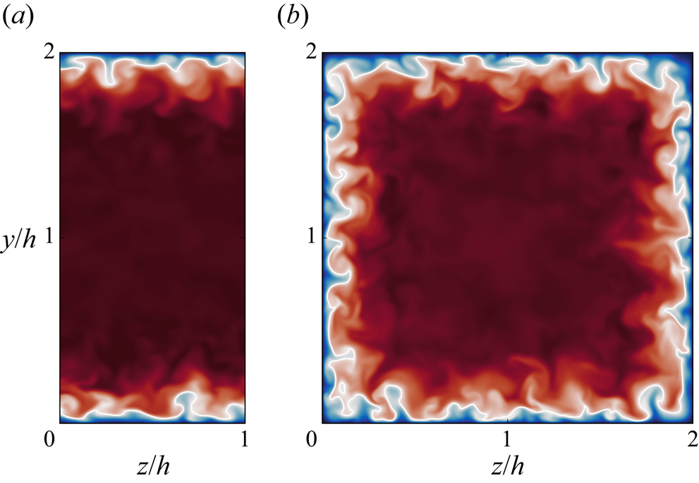
The two sets of cases discussed here were purposefully arranged such that the boundary layers are all the same at the inflow plane, corresponding to  $\delta _{99}/h \approx 0.28$. Thus, the cases have a comparable degree of boundary layer confinement when only considering a slice of the flow along the centreline. Of course, this ignores the 3-D confinement effect of the sidewalls which means that in reality the duct cases are considerably more affected by blockage. This is illustrated in figure 14 which compares the Mach number just upstream of the shock train at $x = 5h$. Although the recorded boundary layer thickness of the duct case is similar to the channel case, it is clear that a much larger proportion of the flow field is contained within the boundary layer region.
Flow cross-sections showing contours of Mach number at  $x = 5h$ for (a) channel and (b) square duct. The sidewalls approximately double the boundary layer blockage.
When comparing ducted flows of different aspect ratios it is useful to define a different confinement ratio which considers additional blockage of the sidewalls. Let this blockage ratio,  $B_{\delta }$, be defined at a given streamwise position as
 \begin{equation} B_{\delta} = \frac{A_{\delta}}{A_{D}}, \end{equation}
where  $\delta$ is an arbitrary measure of boundary layer thickness; $A_{\delta }$ is the cross-sectional area of the boundary layer; and $A_{D}$ is the total cross-sectional area of the duct. For a rectangular duct of width $W$, height $H$, aspect ratio ${AR} = H/W$, and negligible corner thickness effects we find
 \begin{equation} A_{\delta} = 2\delta H (1 + {AR} ^{{-}1}) - 4\delta^2, \end{equation}
and thus with  $A_{D} = HW$ the blockage value can be written as
 \begin{equation} B_{\delta} = (1 + {AR})\frac{\delta}{h} - {AR}\frac{\delta^2}{h^2}. \end{equation}
This relationship only takes into consideration the aspect ratio and the confinement ratio. For the channel arrangement ( ${AR} = 0$) the result reduces to $\delta /h$ and for a square duct ( ${AR} = 1$) and the leading term is ${\sim }2\delta /h$, approximately doubling the blockage. In this connection Reference Vane and LeleVane and Lele (2013) found that doubling the inflow boundary layer thickness of a span-periodic shock train case produced a similar result to including sidewalls.
Boundary layer confinement is known to strongly affect the structure of shock trains. Primarily, the confinement ratio is positively correlated with the shock train length (see for example Reference Carroll, Lopez-Fernandez and DuttonCarroll et al. (1993)). In one key paper (Reference Waltrup and BilligWaltrup & Billig, 1973) an argument was made that the overall length scale of the shock train should scale with the momentum deficit in the viscous layer and that it should have a  $(\theta /D)^N$ dependence for cylindrical ducts ( $D$ being the duct diameter and $N$ a constant). Additionally, Reference Waltrup and BilligWaltrup and Billig (1973) outlined a simple scaling model relating the pressure distribution to the confinement, using the Mach number and Reynolds number just upstream of the shock train, as
 \begin{equation} \frac{(s/h)(M_2^2-1)Re_{\theta}^{1/4}}{(\theta_2/D)^{1/2}} = 50(p/p_2) + 170(p/p_2)^2, \end{equation}
where  $s$ is the streamwise coordinate $x - x_2$ where $x_2$ is the location of the leading edge of the shock train (defined as the location where the wall pressure rises to 5 % above the free stream pressure). This model was further adapted for rectangular ducts (Reference BilligBillig, 1993)
 \begin{equation} \frac{(s/h)(M_2^2-1)Re_{\theta}^{1/4}}{(2\theta_2/h)^{1/2}} = 50(p/p_2) + 170(p/p_2)^2. \end{equation}
Here,  $\theta _2$ is the maximum momentum thickness, taken over all four walls, whereas $h$ is taken as the lower of the duct half-width or half-height. When comparing the two models to results from the literature (see figures 14 and 16 in Reference BilligBillig (1993), for instance) one finds that the cylindrical duct model has a much lower degree of scatter than for rectangular ducts, especially at large pressure ratios. One weakness of the latter model is that no account is made for the aspect ratio of the cross-section (cylindrical ducts do not have this problem). The model predicts identical pressure distributions for different duct geometries which may partially explain the high level of scatter in the data. Here, we propose to replace the momentum thickness ratio $\theta _2/h$ in the Billig model with a momentum thickness-based blockage ratio $B_{\theta _2}$ (i.e. (4.3) with $\delta$ replaced by $\theta _2$), such that the formulation becomes
 \begin{equation} \frac{(s/h)(M_2^2-1)Re_{\theta}^{1/4}}{(2B_{\theta_2})^{1/2}} = 50(p/p_2) + 170(p/p_2)^2. \end{equation}
In figure 15 we plot the pressure distributions of the current work against the unmodified (4.5) and modified (4.6) Billig functions. The polynomial fit on the right-hand side of the equations is included in the figure for reference. For the duct case, the static averaging method is used due to the limited effect of the shock train drift on the wall pressure distribution. The dashed line of the Billig correlation provides a reasonable estimate of the wall pressure through the shock system. Its main limitation (other than the spanwise confinement issue) appears to be that it struggles to follow the shape of pressure rise through the downstream section towards the mixing region (especially for the duct), and thus the overall length of the shock train is unlikely to be well predicted.
Plots of the Billig function against  $p/p_2$ (a) without and (b) with the proposed sidewall correction. The original correlation is shown by the dashed line.
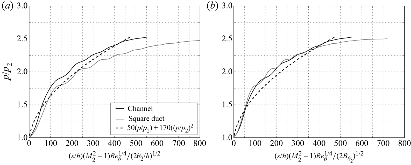
Regarding the modification to the momentum thickness scaling, the gap which initially exists between the channel and duct curves seen in the left-hand figure disappears once the blockage correction is included in the model. This result suggests that there is a rough equivalence between 2-D and 3-D confinement, at least to a first-order approximation. The details are expected to be different, not least due to the presence of additional effects involving secondary flow and corner separations. In an experimental study, Reference Geerts and YuGeerts and Yu (2016a) showed that increasing the blockage by reducing the  $H/W$ aspect ratio elongated the shock train by shifting the leading edge upstream. Contrary to this, Reference Morgan, Duraisamy and LeleMorgan et al. (2014) found reasonable agreement between infinite- and finite-span simulations when the wall pressure distributions were plotted against $x-x_2$, although this may be due to the fact that the upstream boundary layer of the infinite-span case was thicker and that the imposed back pressure was higher. Testing for more aspect ratios as well as different flow conditions may provide better confirmation of the present result.
4.3 Leading shock structure
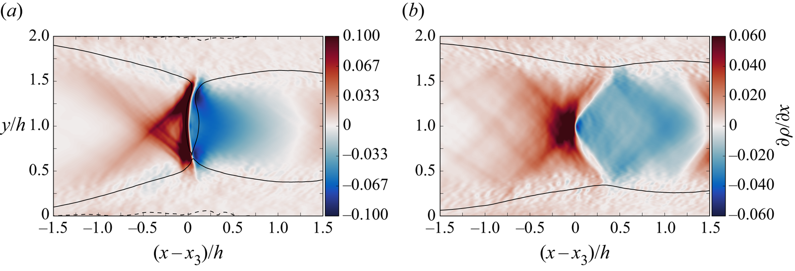
As discussed in § 4.1 the sidewalls have a considerable effect on the strength of the shocks comprising the shock train, where the peak pressure of the leading shocks is significantly reduced compared with the channel case. The structure of the leading shocks is visualised in figure 16 . Here we plot contours of streamwise density gradient at the centreline plane as well as a trace of the  $M=1$ and $M=0$ dividing lines (solid and dashed lines, respectively). Given the sensitivity of the centreline flow, the dynamic averaging method is used for both cases here. The colour scheme allows us to differentiate between regions of flow compression (red) and expansion (blue). While the shock structure in the channel case has a normal component to it (where the most intense compression occurs), the duct case is entirely oblique in nature. Given the rotational symmetry of the cross-section, we may also conclude from this that the shock structure has no planar component and is therefore entirely 3-D.
Contour plots showing centreline, time-averaged streamwise density gradient of the leading shocks of the channel (a) and square duct (b) cases. The solid and dashed lines show  $M=1$ and $M=0$ conditions, respectively. The data capture method compensates for the shock movement. Recordings are taken over approximately two full convective cycles. The different colour ranges accounts for the differing density gradient between the two cases.
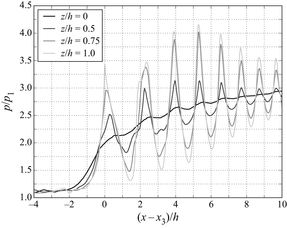
A further examination of the duct case shock structure is presented in figure 17 which shows the static pressure distribution at different spanwise locations. As expected the highest pressure peak occurs at the centreline and the lowest at the wall. The intermediate spanwise locations ( $z=0.5, 0.75h$) show reduced pressure peaks from the centre which is consistent with figure 16(b) where the density gradient is most intense at the confluence of the oblique compression waves.
Variation of static pressure distribution with span (square duct case). The compression and expansion amplitudes decrease towards the sidewalls. The dynamic averaging method is employed here in order to resolve the pressure through the shock waves.
The lack of any large separation zones at the shock train leading edge may help to explain why the peak shock pressures observed in the duct case are considerably lower. A view of the flow deflection through the leading shock is shown in figure 18. It is clear that the flow in the channel case has a significantly larger wall-normal component as it is forced to divert around the separation bubbles on the top and bottom walls. The duct case, in comparison, has significantly less flow deflection due to the fact that no permanent region of reversed flow forms on the centreline. Although the duct case has additional flow deflection in the spanwise direction, the resulting  $(v,w)$ vector still has a lower magnitude to the computed $v$-velocity of the channel case. It follows from this that a lower flow compression occurs at the core of the domain and thus may plausibly explain why a lower shock strength is observed.
Contour plots of centreline  $v$-velocity over the leading shock structure of the channel (a) and duct (b) cases. Flow streamlines are overlaid to illustrate the flow deflection. The dynamic averaging method is used to compensate for the shock movement. Recordings are taken over approximately two full convective cycles.

5. Conclusions
This work presents the results of scale-resolving numerical simulations performed on an enclosed  $M_1=2$ flow. In particular, the effect of sidewall confinement is studied, both on the natural boundary layer development and the behaviour of the shock train which forms in response to an imposed back pressure condition. A grid sensitivity analysis is carried out with and without the back pressure boundary condition in order to establish the sensitivity of various flow properties to the degree of grid resolution. It is found that, while some properties of the turbulent boundary layer (displacement thickness, skin friction) and shock train (equilibrium position) vary with grid resolution, there is a good agreement in terms of the shock train pressure and Mach number distribution.
The first main part of study considers the effect of sidewalls on the unforced boundary layer. Here a span-periodic channel case is compared with a fully enclosed duct with a square cross-section. The duct case involves a considerably higher wall pressure distribution as well as higher boundary layer thickness and skin friction. Despite these differences, surprisingly little change is observed with the van Driest-scaled boundary layer profiles and density-scaled Reynolds stress profiles. As expected, the time-averaged flow field of the square duct case exhibits strong counter-rotating corner vortex pairs (Prandtl secondary flow).
A counterpart study is performed with the presence of shock trains. Here, the square duct case shock train is considerably longer than that of the channel case and is composed of a higher number of shocks. Despite the presence of the large pressure gradient and shock waves, the corner vortices are once again observed with equal or greater strength to those of the unforced case. To provide an explanation for the longer shock train caused by the sidewalls, a blockage ratio parameter is introduced. Using this blockage ratio in place of the momentum thickness term in the Reference BilligBillig (1993) shock-train model, an improved agreement is found between the channel and duct pressure distributions. This suggests an equivalence between 2-D and 3-D confinement in shock train problems.
Finally, a comparison between the leading shock structures is presented. In addition to the lower peak shock pressure, the duct case also lacks a normal shock component and is instead entirely oblique in nature. On the other hand the leading shock in the channel case has a compound normal and oblique structure. Despite a very similar wall pressure gradient through the first shock, only the channel case exhibits a large separation bubble (the duct case only has a permanent separation in the corner regions). This is likely due to the higher wall skin friction in the latter cases which allows it to resist boundary layer separation more easily. Additionally, it is suggested that this lack of separation causes a lower degree of flow deflection, thus explaining the weaker shocks which are observed.
Supplementary material
Supplementary material is available at https://doi.org/10.1017/flo.2023.6.
More detail of the grid sensitivity study can be found in the supplement. Time-averaged shock train and boundary layer data can be found at https://doi:10.5258/SOTON/D1770. Request for additional data should be made to the corresponding author (A.M.G.). The OpenSBLI code is available at https://opensbli.github.io.
Acknowledgements
The authors would like to thank Dr S. Shaw of MBDA UK, who provided feedback and advice throughout the course of the project.
Declaration of interests
The authors declare no conflict of interest.
Funding statement
A.M.G. acknowledges the support of MBDA UK who funded his PhD programme at the University of Southampton. All of the simulations in the current work were conducted at the University of Cambridge HPC facility and the authors are grateful to the Cambridge Service for Data Driven Discovery (CSD3) for providing the computational resources (EPSRC Tier-2 capital grant EP/P020259/1).
Author contributions
A.M.G. and N.D.S. created the research plan. A.M.G. ran the simulations and performed the post processing of the data. A.M.G. and N.D.S. wrote the manuscript.


 Open access