


1. Introduction
Patagonia (40–55° S) comprises the most extensive icefields at mid-latitudes in the Southern Hemisphere: the Southern Patagonia Icefield (SPI) and the Northern Patagonia Icefield (NPI). Glacier wastage in this region (Rignot and others, Reference Rignot, Rivera and Casassa2003; Davies and Glasser, Reference Davies and Glasser2012; Willis and others, Reference Willis, Melkonian, Pritchard and Rivera2012; White and Copland, Reference White and Copland2015; Foresta and others, Reference Foresta2018; Malz and others, Reference Malz2018; Abdel Jaber and others, Reference Abdel Jaber, Rott, Floricioiu, Wuite and Miranda2019; Braun and others, Reference Braun2019; Dussaillant and others, Reference Dussaillant2019) is a matter of concern due to its observed and potential contribution to sea-level rise (Gardner and others, Reference Gardner2013; Zemp and others, Reference Zemp2019; Masiokas and others, Reference Masiokas2020) and the role of receding glaciers in triggering hazardous natural events such as glacial-lake outburst floods (Wilson and others, Reference Wilson2018) and rock avalanche events associated with de-buttressing (Iribarren-Anacona and others, Reference Iribarren-Anacona, Mackintosh and Norton2015).
The SPI is the largest continuous ice mass along the Andes with a total area of 12 232 ± 201 km2 (Meier and others, Reference Meier, Grießinger, Hochreuther and Braun2018, Fig. 1). The large glaciers are mostly lacustrine-calving towards the east and marine-terminating to the west. This icefield has been the focus of several geodetic mass-balance estimates in recent years. Despite some differences in their magnitude and spatial variability, these geodetic mass balances agree that the SPI as a whole is losing mass, irrespective of the observation period (e.g. Rignot and others, Reference Rignot, Rivera and Casassa2003; Willis and others, Reference Willis, Melkonian, Pritchard and Rivera2012; Malz and others, Reference Malz2018; Braun and others, Reference Braun2019; Dussaillant and others, Reference Dussaillant2019). However, a number of glaciers in the SPI are stable, so a glacier response is best described as heterogeneous (Foresta and others, Reference Foresta2018; Abdel-Jaber and others, Reference Abdel Jaber, Rott, Floricioiu, Wuite and Miranda2019). Dynamical adjustments associated with calving glaciers have been invoked as a key control of the overall ice losses (Mouginot and Rignot, Reference Mouginot and Rignot2015; Braun and others, Reference Braun2019) supported by observations that land-terminating glaciers outside the icefields show less mass loss (e.g. Falaschi and others, Reference Falaschi2017, Reference Falaschi2019) despite being exposed to the same climatic forcing (Braun and others, Reference Braun2019). Moreover, surface mass-balance modelling forced with climate data shows positive mean values for the entire SPI (Schaefer and others, Reference Schaefer, Machguth, Falvey, Casassa and Rignot2015; Mernild and others, Reference Mernild, Liston, Hiemstra and Wilson2016), leading to questions around how the mass balance of glaciers in this region will evolve over coming decades.
Studies based on direct in situ observations that characterise the fundamental meteorological and glacier conditions needed for surface mass balance and energy-balance models are, however, extremely limited in number in this region (Masiokas and others, Reference Masiokas2020). Direct mass-balance measurements using the glaciological method are equally scarce. This means that high uncertainty exists in earlier modelling efforts, as no on-glacier observations have been available to validate the meteorological variables used to drive and parameterise these models (e.g. Schaefer and others, Reference Schaefer, Machguth, Falvey, Casassa and Rignot2015; Mernild and others, Reference Mernild, Liston, Hiemstra and Wilson2016). Additionally, efforts to estimate the sensitivity of these glaciers to climate changes have been made using coarse-climate models and re-analysis (e.g. Cook and others, Reference Cook, Yang, Carter and Belcher2003; Rasmussen and others, Reference Rasmussen, Conway and Raymond2007; Sagredo and Lowell, Reference Sagredo and Lowell2012) which do not capture the finer details and spatial differences of the drivers of the surface mass balance. Consequently, our understanding of how glaciers are responding to changes in climate over this important region of the Andes is limited (Pellicciotti and others, Reference Pellicciotti, Ragettli, Carenzo and McPhee2014).
A notable characteristic in Patagonia that defines the meteorological conditions is the orographic effect. This effect has been described at a regional scale, especially in terms of precipitation and water vapour. Due to the mechanical effect of the mountain chain, the air ascends in the western sector (windward) favouring conditions for saturation and hence the occurrence of precipitation, while subsidence of the air and inhibition of the precipitation occurs in the eastern sector (leeward) (Schneider and others, Reference Schneider2003; Smith and Evans, Reference Smith and Evans2007; Garreaud and others, Reference Garreaud, Lopez, Minvielle and Rojas2013; Lenaerts and others, Reference Lenaerts2014). However, it seems that the orographic effect also has direct effects at the scale of the SPI, forcing meteorological conditions that are distinct from one side of the icefield to the other.
The most evident impact of the orographic effect is the difference in cloud cover and its impact on the magnitude of the incoming shortwave radiation on both sides of the SPI (Schaefer and others, Reference Schaefer, Machguth, Falvey, Casassa and Rignot2015). It has been shown that distinct lapse rates prevail between western and eastern glaciers which in turn has implications for the estimation of surface ablation (Bravo and others, Reference Bravo2019a). Additional insights of the spatial differences in the SPI come from remote-sensing analyses, which suggest the influence of humid conditions is manifested by differing snow facies on either side of the divide (De Angelis and others, Reference De Angelis, Rau and Skvarca2007) and also in differences in the timing of melt season onset, being earlier in the west compared to the east (Monahan and Ramage, Reference Monahan and Ramage2010).
To assess how the meteorological differences forced by the orographic effect impact surface ablation, we present a distributed surface energy balance (SEB) model for glaciers located in the northern section of the SPI (48–49° S) and on both sides of the divide. The aim is to increase our understanding of the processes and fluxes controlling surface ablation and its spatial differences. For this purpose, we used meteorological observations collected by automatic weather stations (AWSs) between October 2015 and June 2016 at several locations (Fig. 1).
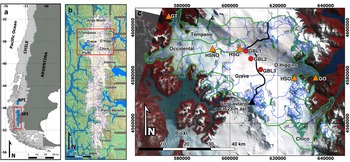
(a) Southern South America, NPI and SPI are the Northern and Southern Patagonia Icefields, respectively. (b) SPI overlying a hillshade map of the region obtained from SRTM. (c) Study area and locations of the observational network in a Landsat-8 OLI acquired on 1 April 2014. Symbols are AWSs (triangles) and GBL stations (red circles). Green lines denote the glacier boundaries and black line is the ice divide. Image coordinates are UTM18-S, WGS-1984.

2. Materials and methods
2.1. Automatic weather stations
The observational network consists of five AWSs installed in proglacial zones and nunataks on the plateau of the SPI along a west–east transect ~48° S (Fig. 1). Also, three air temperature sensors and ultrasonic depth gauges (UDGs) were installed over the glacier surface in the so-called Glacier Boundary Layer stations (GBL; Fig. 1 and Table 1). The UDGs at GBL1 and GBL2 were primarily used to compare with our computed ablation values. The broader network allowed us to describe the spatial and temporal variabilities under meteorological conditions, as well as to calculate the components of the SEB. Table 1 shows the details of each AWS, including the sensors and locations. Details of the characteristics of the locations of each AWS are given in Bravo and others (Reference Bravo2019a).
Locations and details of the sensors for each AWS

n/a, not available measurements.
2.2. Distribution of meteorological variables
The spatial coverage of the AWS network made it possible to distribute the meteorological variables that were needed to force the SEB. We used elevation gradients as the main method of spatial distribution of meteorological variables (Table 2). TanDEM-X digital elevation data acquired by the German Aerospace Center (DLR) in the years 2012 and 2015 (Abdel-Jaber and others, Reference Abdel Jaber, Rott, Floricioiu, Wuite and Miranda2019) and gridded at 200 m resolution, were used to distribute the meteorological variables and to estimate radiation fluxes. The glacier outlines were obtained from the inventory of De Angelis (Reference De Angelis2014), but frontal positions and margins were manually updated based on a cloud-free Landsat-8 OLI satellite image acquired on 1 April 2014.
Methods, assumptions and approach references used to distribute the meteorological data over the glaciers on the SPI

The meteorological variables and factors related to cloud cover were taken from the AWS observations (Table 1). We assumed that the AWS observations installed on the west side (GT, HSNO) were representative of glaciers Témpano (327 km2), Occidental (218 km2), Greve (412 km2), HPS8 (34 km2) and one unnamed glacier (41 km2). AWSs installed on the east side (GO, HSO) were considered representative of glaciers O'Higgins (751 km2), Pirámide (27 km2) and Chico (229 km2). HSG AWS was considered as representative of the conditions at the ice divide.
Air temperature was distributed using hourly lapse rates between each pair of AWS. A bias-correction was applied considering that the observations were taken on relatively small rock surfaces surrounded by ice (nunataks), meaning that the glacier cooling effect (i.e. cooling of the near-surface air layers in comparison with the ambient off-glacier conditions and induced by the glacier surface; Carturan and others, Reference Carturan, Cazorzi, De Blasi and Dalla Fontana2015) is not included directly in the air temperature observations. Based on the findings of Bravo and others (Reference Bravo2019a), the bias-correction applied was 1°C at the west side and 3°C at the east side. Further details of the air temperature observations, lapse rates and bias-correction are given in Bravo and others (Reference Bravo2019a).
The AWS network offered the possibility to distribute humidity, rather than assume a constant value (e.g. Braun and Hock, Reference Braun and Hock2004; Fyffe and others, Reference Fyffe2014). Considering the extreme meteorological gradients observed in the Patagonian region, an adequate representation of the humidity conditions at both sides of the SPI is critical to increasing our understanding of the meteorological factors controlling ablation. The distributed relative humidity was calculated using air vapour pressure (e a) and air saturation vapour pressure (e sat) as separate components. For each AWS, we calculated the air water vapour pressure, using the observed (2 m) relative humidity (f) and air temperature (T a), as follows:

where e sat according to the empirical formula of Clausius–Clapeyron (Bolton, Reference Bolton1980), is only a function of T a in °C:

Air water vapour pressure was fitted against elevation (Shea and Moore, Reference Shea and Moore2010) and hourly gradients were obtained. Mean gradient values of the air water vapour pressure were −0.84 hPa km−1 on the east side and −2.80 hPa km−1 on the west side. Typical values of hourly gradients observed in glaciers elsewhere were between −6 and −1 hPa km−1 (Shea and Moore, Reference Shea and Moore2010). Hence, our eastern gradient was slightly outside this typical range.
The atmospheric pressure was distributed using the hydrostatic equation (Wallace and Hobbs, Reference Wallace and Hobbs2006) that relates two elevations and pressure levels and allows correction of the atmospheric pressure to a reference level (e.g. sea level).
To estimate the surface temperature (T s), we used as a proxy the dew point temperature (T d) for the snow surface and the assumption of constant surface temperature (0°C) under melt conditions on glacier surfaces, namely when the air temperature is positive (Oerlemans and Klok, Reference Oerlemans and Klok2002). The T d approach calculated at a standard height is a reasonable first-order approximation of daily T s (Raleigh and others, Reference Raleigh, Landry, Hayashi, Quinton and Lundquist2013), but here it was computed at hourly time step using the Magnus–Tetens approach (Murray, Reference Murray1967, Raleigh and others, Reference Raleigh, Landry, Hayashi, Quinton and Lundquist2013):

As the aim was to estimate snow surface temperature when T a<0°C, the coefficients used were b = 22.587 and c = 273.86°C (Raleigh and others, Reference Raleigh, Landry, Hayashi, Quinton and Lundquist2013). Figure S1 shows the relationship between air temperature and dew point temperature for different values of relative humidity.
When the air temperature was equal to zero or positive, the snow/ice surface temperature was fixed to 0°C and the surface water vapour pressure (e s) was fixed to 6.11 hPa assuming saturation (Brock and Arnold, Reference Brock and Arnold2000). Under sub-zero conditions, we assume saturation of the surface layer. The surface water vapour pressure therefore depends only on the surface temperature and was calculated according to Eqn (2).
Finally, the wind speed was distributed using the hourly observed gradients between the pairs of AWS. On the west side, the gradients were taken from GT and HSNO and on the eastern side from GO and HSO. This approach has also been used by Fyffe and others (Reference Fyffe2014) on alpine glaciers. However, due to the uncertainties of this approach (as wind speed is also related to local topographic characteristics), we used a constant wind speed to check the sensitivity of the SEB model to this variable. Here, the wind speed measurements at the mid-elevation AWS, HSNO and HSO (Table 1), were assumed representative of the west side and the east side, respectively. Table 2 shows a summary of the methods to distribute meteorological variables including the time step and related references.
2.3. SEB model
A distributed SEB model was applied using the distributed meteorological fields (section 2.2) based on the AWS data collected between 1 October 2015 and 31 June 2016 (Table 1). The time step used in the SEB model was hourly, even though the approach to surface temperature estimation (Eqn (3)) is recommended for daily data (Raleigh and others, Reference Raleigh, Landry, Hayashi, Quinton and Lundquist2013). The energy available for melting, Q m (W m−2), was determined following the equation:

where S in and α are incoming shortwave radiation and albedo, L in and L out are incoming and outgoing longwave radiation and Q h and Q l are the turbulent fluxes of sensible and latent heat, respectively. Q r is the sensible heat brought to the surface by rain. The conductive heat flux was considered negligible due to the predominantly positive air temperatures and the temperate conditions of the glacier surface (e.g. Schneider and others, Reference Schneider, Kilian and Glaser2007; Gillett and Cullen, Reference Gillett and Cullen2010; Schwikowski and others, Reference Schwikowski, Schläppi, Santibañez, Rivera and Casassa2013).
After computing the energy available for melt, the surface ablation was calculated as the sum of the surface melt and sublimation. Melt was assumed to occur only when the glacier surface was at 0°C and Q m was positive. The melt rate (M) was calculated as follows:

where L m is the latent heat of fusion and ρ w is the water density (1000 kg m−3).
The sublimation rate (S) was calculated as follows (Cuffey and Paterson, Reference Cuffey and Paterson2010):

where L s is the latent heat of sublimation. The negative values of latent heat fluxes (Q l) under negative surface temperature correspond to sublimation (Ayala and others, Reference Ayala, Pellicciotti, Peleg and Burlando2017).
2.4. Shortwave and longwave radiation fluxes
Distributed global radiation was derived using a radiation model in a GIS environment (Fu and Rich, Reference Fu and Rich2002) and using TanDEM-X digital elevation data. Global radiation comprises direct and diffuse solar radiation and was computed under a clear-sky assumption with bulk atmospheric transmissivity equal to 1, to represent the potential clear sky shortwave radiation S in,pot at each gridpoint. The potential clear-sky shortwave radiation was corrected using the bulk atmospheric transmissivity (τ atm) derived from the relationship between the potential and the observed shortwave radiation at the location of each AWS (Sicart and others, Reference Sicart, Hock, Ribstein and Chazarin2010). In the cases when observed values are higher than potential values (probably due to instrument malfunction), atmospheric transmissivity was assumed to be equal to 1. The bulk atmospheric transmissivity was spatially distributed (τ atm,dis) as a linear relationship with elevation on each side of the SPI (e.g. see data presented in Fig. S2). Hence, the incoming shortwave radiation at the glacier surface is (S in,gla):

The albedo of the glacier surface was estimated using the model of Oerlemans and Knap (Reference Oerlemans and Knap1998). This model assumes that albedo depends on the age of the snow surface and depth. To estimate the snow accumulation on the glacier surface we used the total precipitation data from ERA5-Land (9 km) (Muñoz-Sabater and others, Reference Muñoz-Sabater2021) resized to 200 m using a nearest neighbour method. The snow accumulation was estimated using the phase partitioning methods (PPMs) proposed by Weidemann and others (Reference Weidemann2018) which showed a close fit between modelled and observed accumulation rates, with observations coming from UDGs within the study area and presented in Bravo and others (Reference Bravo2019b). The air temperature used to define the partitioning was not bias-corrected as we assumed that the contributing snow mass is formed entirely outside the GBL. In this case, the comparison between ERA5-Land derived accumulation and the UDGs (GBL stations; Fig. 1, Table 1) derived accumulation, while not perfect (see Fig. S3), shows a good linear relationship, reaching an r value of 0.73 for the UDG installed at GBL2 (1294 m a.s.l.) and 0.55 for the UDG installed at GBL1 (1415 m a.s.l.). This means that there is a similar inter-daily variability between both datasets. The total accumulation estimated in GBL1 was 0.9 m w.e. using ERA5-Land data and 1.1 m w.e. using the UDG. This latter value was also reported by Durand and others (Reference Durand2019) at the same location and for a similar period. Then the albedo is estimated using the relationships (Oerlemans and Knap, Reference Oerlemans and Knap1998):


where α t corresponds to the global albedo at the surface on a specific day t. $\alpha _{\rm s}^t$ corresponds to the snow albedo at the surface on day t. The parameters α fr and α fi represent fresh snow albedo (0.85) and firn or old snow albedo (0.53), respectively. α ice represents a specific glacier ice albedo (0.35), while t* corresponds to the timescales that represent the transition of fresh snow albedo to firn (3 days). The term Δt refers to days since the last snowfall event. The parameters d and d* correspond to the snow depth (in m), and scale coefficient of snow depth (0.032 m), respectively.
To validate the surface albedo output estimated by the model, we used albedo values derived from available (e.g. cloud-free) Landsat-8 OLI satellite images during the same period at a spatial resolution of 30 m. Processing of the Landsat imagery is described and explained in the Supplementary material. Overall, the modelled albedo replicated the elevational gradient of the Landsat-8-derived albedo (Fig. 2a,b), but without some of the finer details, partly due to the differences in resolution. The greatest differences were concentrated on the glaciers at mid-elevation on each side of the SPI, probably related to the exact location of the snowline. The albedo from Landsat was also used to define the albedo of the supraglacial moraines observed on the glacier ablation zone of the study area. Hence, the albedo of the supraglacial moraine was obtained from the Landsat-8 images acquired on 8 March 2016 and was prescribed for each day depending on the snowline elevation. As albedo was computed at daily time step, to coincide with our other hourly data, we assumed this value was constant throughout the day due to its slow evolution.
Comparison of the observed albedo using Landsat-8 satellite images (a) and modelled albedo using Oerlemans and Knap (Reference Oerlemans and Knap1998) approach (b). Albedo values on supraglacial moraine in (b) were prescribed.

Incoming longwave radiation (L in,gla) was estimated using the Stefan–Boltzmann law (i.e. Mölg and others, Reference Mölg, Cullen and Kaser2009; Ayala and others, Reference Ayala, Pellicciotti, Peleg and Burlando2017):

where σ is the Stefan–Boltzmann constant and S vf is the sky-view factor calculated (Oke, Reference Oke1987) with the TanDEM-X digital elevation data. S vf varied between 1 in the lower slope zones of the plateau and ~0.55 in the higher slopes. Atmospheric emissivity for all-sky conditions (ɛatm) was calculated as the product of clear-sky emissivity (ɛatm,clear) and the cloud factor (F cl). The cloud factor was obtained as the ratio of the observed and the clear-sky incoming longwave radiation at the location of two representative mid-elevation AWS, HSNO on the west side and HSO on the east side. In this case, it was assumed that the cloud factor is representative of the total area of the glaciers on each side. Meanwhile, the clear-sky emissivity was estimated using the spatially distributed fields of air temperature (K) and the water vapour pressure (hPa) using the Brutsaert (Reference Brutsaert1975) expression:

where P 1 = 1.24 and P 2 = 7.
The outgoing longwave radiation was calculated using the distributed field of surface temperature and assuming a surface emissivity equal to 1 in the Stefan–Boltzmann law.
2.5. Sensible, latent and rainfall heat fluxes
The turbulent heat fluxes were calculated using the bulk approach (Cuffey and Paterson, Reference Cuffey and Paterson2010). In the case of the sensible heat flux:

where u is the wind speed in m s−1, T a is the air temperature in K and T s is the glacier surface temperature. C* is a dimensionless transfer coefficient, which is a function of the surface aerodynamic roughness (z 0):

where z is the height above the surface of the T a and u measurements (2 m) and k is the von Kárman's constant (0.4). Due to the absence of microtopographic measurements, z 0 was prescribed according to the albedo using values taken from Brock and others (Reference Brock, Willis and Sharp2006) (Table S1). This is a general approximation to estimate the surface roughness as, for instance, wind speed is not considered, while in the aerodynamic method it is used for fitting the wind profile to determine z 0 (Chambers and others, Reference Chambers2020). However, it has been suggested that surface roughness also affects surface albedo, especially on snow surfaces (Manninen and others, Reference Manninen, Lahtinen, Anttila and Riihelä2016).
ρ a is the density of air, which depends on atmospheric pressure P (in Pa):

where $\rho _{\rm a}^0$ (1.29 kg m−3) is the density at standard pressure P 0 (101300 Pa). Finally, c a is the specific heat of air at constant pressure (J kg−1 K−1) calculated as follows (Brock and Arnold, Reference Brock and Arnold2000):

The latent heat flux Q l is

where e a is the water vapour pressure in the air, e s is the water vapour pressure at the glacier surface (Brock and Arnold, Reference Brock and Arnold2000) and both were estimated using Eqns (1) and (2) but at distributed scale. L v/s is the latent heat of vaporisation or sublimation, depending on whether the surface temperature is at melting point (0°C) or below the melting point (<0°C), respectively.
Stability corrections were applied to turbulent fluxes using the bulk Richardson number (Ri b), which is used to describe the stability of the surface layer (Oke, Reference Oke1987):

where g is the acceleration due to gravity.
For Ri b positive (stable)

For Ri b negative (unstable)

The rain heat flux (Q r) is a function of the rainfall rate intensity (R, m s−1) and the rain temperature (T r) is assumed to be equal to the air temperature (Hock and Holmgren, Reference Hock and Holmgren2005; Gillett and Cullen, Reference Gillett and Cullen2010):

where ρ w is the density of water and c w is the specific heat of water (4180 J kg−1 K−1). The rainfall intensity was obtained from the total precipitation ERA5-Land dataset at a daily time step. The rainfall was obtained from the total precipitation using four PPMs (Koppes and others, Reference Koppes, Conway, Rasmussen and Chernos2011; Ding and others, Reference Ding2014; Schaefer and others, Reference Schaefer, Machguth, Falvey, Casassa and Rignot2015; Weidemann and others, Reference Weidemann2018) as explained in Bravo and others (Reference Bravo2019b).
3. Results
3.1. Meteorological conditions: observations and distribution
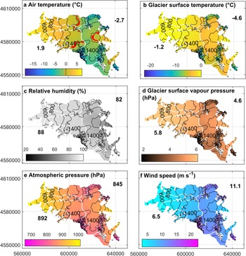
At comparable elevations, off-glacier air temperatures were higher in the east compared to the west, as the mean value of HSO (1234 m a.s.l.) was similar to HSNO (1040 m a.s.l.), although the former was located at a higher elevation (Fig. 3a). As expected, distributed on-glacier air temperature and distributed glacier surface temperature were lower on the east side compared to the west side due to a strong cooling effect, which has been observed in a previous study (Bravo and others, Reference Bravo2019a). In the ablation zones, mean glacier surface temperatures were close to 0°C (and surface water vapour pressure close to 6.11 hPa; Figs 4b, d). Lo Vecchio and others (Reference Lo Vecchio2019) estimated colder surface temperatures using MODIS products in the lower part of O'Higgins Glacier, reaching −2.4 to −5.2°C between 500 and 1300 m a.s.l., while our estimation for the same elevation range was between −0.1 and −1.7°C. Western-facing glaciers comprised of a larger elevation range below the 0°C isotherm (Fig. 4a).
Boxplot summaries of the hourly observed meteorological variables in the SPI during the period October 2015 to June 2016. Data used in the incoming shortwave radiation boxplots (e) correspond to observed hourly values over 5 W m−2. Upper and lower box limits are the 75 and 25% quartiles, the horizontal line is the median, the filled black circle is the mean, whiskers are extreme values not considered outliers and red crosses are outlying values (more than 1.5 times the interquartile range away from the bottom or top of the box).

Spatially distributed mean values of the meteorological variables during the period October 2015 to June 2016. Numbers shown in each variable map represent mean glacier-wide values for each side of the icefield. White lines are the glacier divide and black lines are contours at an interval of 200 m. Coordinates are in m, UTM18-S, WGS-1984.

Relative humidity shows different behaviours between each side of the SPI (Figs 3b, 4c). On the west side, the relative humidity shows low-spatial variability as the observed mean values tend to be similar irrespective of elevation (Fig. 3b). On the eastern side, lower mean values were observed and a strong gradient between HSO (mean of 78% during the nine months period) and GO (mean of 57%) was determined (Fig. 3b). Following this pattern, distributed relative humidity and surface water vapour pressure (Figs 4c, d) show, overall, drier conditions in the east in comparison with the west.
The wind speed (Figs 3c, 4f) increases with elevation on the west side while the maximum values were observed at mid elevations of the eastern side (HSO), reaching a mean of 9 m s−1 but with maximum hourly means reaching 25–30 m s−1 at this location. Lower mean values were observed at the lower elevations on the western side. Distributed wind speed reached a maximum spatial mean of ~22 m s−1 (Fig. 4f) at the highest elevation of the study area (Volcán Lautaro ~3600 m a.s.l.). The wind speeds, we estimated here (after using the observed gradient), are comparable to those determined by Lenaerts and others (Reference Lenaerts2014) using the regional atmospheric climate model RACMO2 at a level of 700 hPa.
3.2. SEB fluxes
The observed incoming shortwave radiation showed differences on either side of the divide (Fig. 3e). Lower values were observed on the western side, especially at GT and HSNO. On the ice divide (HSG), the incoming shortwave radiation showed the maximum values, followed by the eastern side AWS (HSO, GO). Higher values were due to the period between December 2015 and April 2016 being characterised by positive solar radiation anomalies increasing the insolation by ~20% compared to the annual climatology (Garreaud, Reference Garreaud2018). However, we cannot discard some outlier values due to erroneous measurements. The observed incoming longwave radiation values were larger in the west than in the east; HSNO in the west (1040 m a.s.l.) and GO in the east (310 m a.s.l.) showed similar values despite the elevation differences. The differences in magnitude that are evident in incoming shortwave and longwave radiation values either side of the divide can be attributed to differences in the cloud cover, being more persistent on the west side.
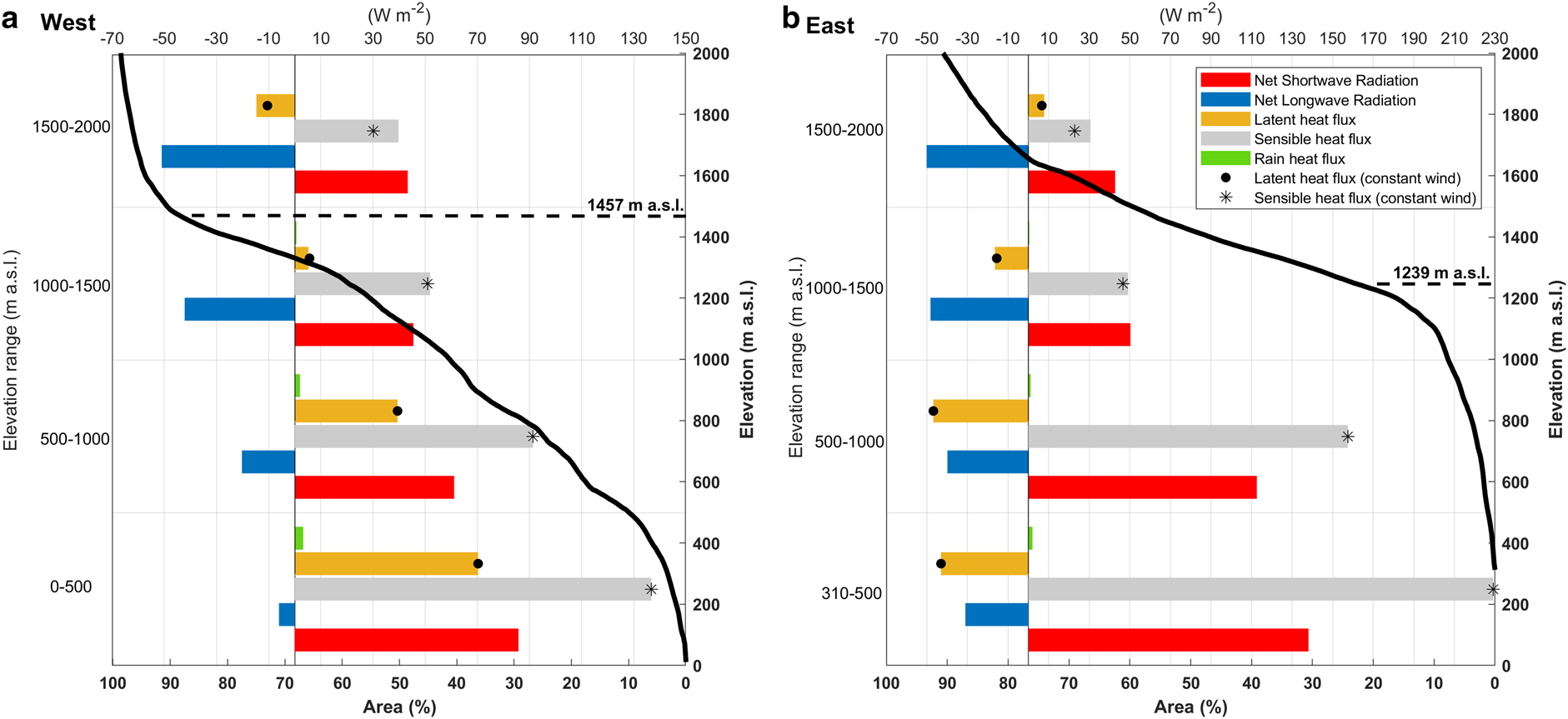
The distributed spatial and temporal mean SEB fluxes modelled for the period between October 2015 and June 2016 per elevation range until 2000 m a.s.l. are shown in Figure 5, while the maps of the distributed mean fluxes over the study period are presented in Figure 6. Overall, across all the glacier surfaces, net shortwave radiation, sensible heat flux and rain heat flux were positive, which means that they were a source of energy available for surface melt and heating.
Mean values of the energy-balance fluxes per elevation range and margin of the SPI during the period between October 2015 and June 2016, focused on the elevations where most of the melt occurs and most of the glacier area is concentrated: (a) west and (b) east. For reference, hypsometric curves (black continuous line) estimated using the TanDEM-X data with the accumulated area in the bottom axis and the elevations in the left axis are shown along with the mean elevation of the isotherm 0°C (dashed line).
Distributed mean values of the energy-balance fluxes estimated over the period October 2015–June 2016. Values are the glacier-wide mean for each flux. White lines are the glacier divide and black lines are contours at an interval of 200 m. Coordinates are in m, UTM18-S, WGS-1984.

Sensible heat flux was, overall, the dominant source of energy on both sides, even assuming constant wind speed (Fig. 5). However, at elevations between 1000 and 2500 m a.s.l. in the west and above 1500 m a.s.l. in the east, the absolute value was similar to the net shortwave and longwave radiation. The sensible heat flux showed larger positive values on the lower elevations of the east side. This area was characterised by a strong temperature gradient between the glacier surface (fixed at 0°C for most of the period; Fig. 4b) and the air (4–5°C; Fig. 4a), and relatively strong winds. However, the maximum values correspond to the supraglacial moraine areas, where we assumed highest surface roughness; thus, the value depends on the fixed surface roughness. For instance, on the ice surface areas in the frontal section, the mean sensible heat flux reached a value of ~190 W m−2 while on the supraglacial moraine surfaces it reached a mean value of ~220 W m−2 (Fig. 6d). This 30 W m−2 of enhanced sensible heat corresponds to a difference in surface roughness of only 0.006 m in the sensible heat flux computation.
The net shortwave radiation was the second highest flux at the lower elevations (<1000 m a.s.l.), but the magnitude on the east side, where clear skies prevail, in comparison with the west side, was higher by ~40–50 W m−2. Due to a relatively high albedo in the east (mean 0.77) compared to the west (0.67), the spatial mean net shortwave radiation was almost identical between both sides; 54 W m−2 to the west and 52 W m−2 to the east (Fig. 6). The net shortwave radiation showed a relative maximum in the supraglacial moraine area as a reduction in albedo occurs (Fig. 6a).
Net longwave radiation was negative across almost all the glacier surface, hence removing energy. The exception to this was in the lower elevations of the west side, where near-constant cloud cover and positive temperatures prevailed over the analysed period (Fig. 6b). In terms of spatial mean values (Fig. 5), in the western lower elevations, incoming longwave radiation reached values comparable to the emitted longwave radiation, which most of the time was at 315 W m−2 as the glacier surface was at the melting point. Hence, the net longwave radiation was close to zero in this area. At the same elevation on the eastern side, the cloud cover was lower, and less water vapour was in the atmosphere, hence the incoming longwave radiation was predominantly lower than the emitted, as the glacier surface was still close to the melting point most of the time. Above an elevation of 1000 m a.s.l., the net longwave radiation becomes more negative on both sides, and even becomes the flux with the highest absolute value between 1500 and 2500 m a.s.l. on the western side.
The latent heat flux (Fig. 6c) demonstrated the largest spatial variability, with positive values estimated on the west side and negative values on the east side consistent with the relatively dry conditions and strong wind speed on the east side. The latent heat flux was therefore a sink of energy until 1500 m a.s.l. on the eastern side, whereas on the western side it was a source of energy up to ~1500 m a.s.l. (Fig. 5).
The rain heat flux showed maximum values on the west side where more rainfall occurs, but reached a spatial and temporal mean of just 4–5 W m−2 with daily maxima ~11 W m−2.
As might be expected, the maximum values (>300 W m−2) of energy available for melt/heating were at lower elevations on each side, decreasing to values lower than 100 W m−2 in most of the plateau area. Glacier-wide mean values were considerably higher in the west (115 W m−2) compared to the east (50 W m−2) (Fig. 6f).
3.3. Surface ablation
The computed ablation shows good agreement with the magnitude of the ablation estimated with the GBL stations (Fig. S4), but with some differences in the variability and the magnitude of some events. Unfortunately, these sensors only captured data for 3 months in the case of GBL1 and 2 months in the case of GBL2. The surface melt was the dominant ablation component over most of the glacier area on both sides (Fig. 7). Comparatively, the magnitude was higher in the west, especially in the range between 1000 and 2000 m a.s.l. where mean differences were in the range of 1–4 m w.e. when compared to the east side. On the eastern side, between 1000 and 1500 m a.s.l., melt was approximately half of the melt on the west side. In this elevation range, the eastern side melt decreased sharply to <5 m w.e. above 1000 m a.s.l., hence, most of the melt on eastern side glaciers was observed around their termini. On the western side, surface melt >10 m w.e. was observed up to an elevation of ~900 m a.s.l.
Total modelled melt and sublimation over the whole period. (a) West, melt and sublimation (black circles) vs elevation. The colour of each melt point denotes the albedo used in the SEB model and the grey line is the glacier hypsometry with the area per 100 m bin. (b) Same as (a) but for the eastern margin glaciers. Grey points correspond to the melt computed by Schaefer and others (Reference Schaefer, Machguth, Falvey, Casassa and Rignot2015) and represent the mean for the period 1975–2011. Zones of supraglacial moraine where albedo reduction and enhanced melt occurs are indicated on both sides.
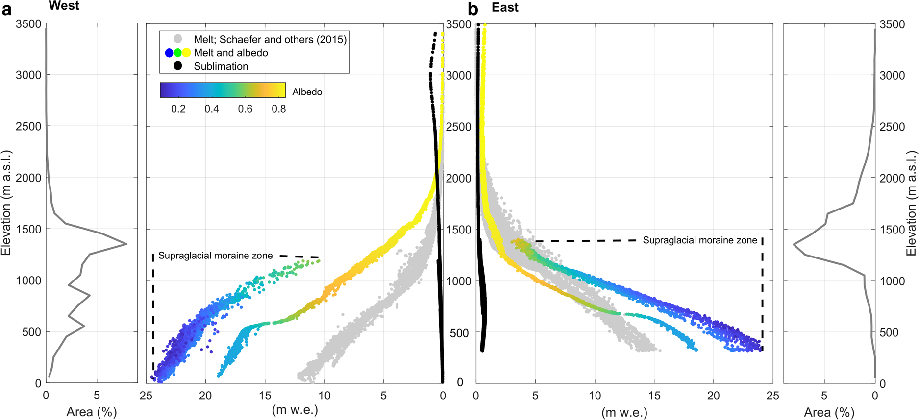
On both sides, and due to a local reduction in surface albedo, the maximum melt occurred at supraglacial moraine areas on the lower sections (marked curves in Fig. 7) reaching maximum values on the order of 24 m w.e. Melt in supraglacial moraine areas was 2–5 m w.e. higher than melt in debris-free areas at the same elevations (Fig. 7). At the glacier scale, melt reached 9.3 m w.e. (8.5 m w.e.) on the west side and 2.9 m w.e. (2.4 m w.e.) on the east side depending on the inclusion (or not) of the moraine albedo parameterisation (Fig. 2). Hence, the impact of the moraine albedo parameterisation was relatively higher on the eastern side as melt increased by 17%, while in the west, it increased by 9%.
The impact of using constant wind speed, obtained from the mid-elevation AWS at each side, is minimal on the surface ablation. The glacier-wide surface ablation on the western side was reduced by 0.4%, while on the eastern side it was reduced by 2%.
The percentage of glacier-wide sublimation compared to net ablation in the west was 1.9% and in the east it was 5.4%. Spatial differences were observed when comparing both sides. On the west side, sublimation was the main component of the surface ablation at elevations over 2000 m a.s.l., which corresponds to an area of 2% (Fig. 7a). Meanwhile, eastern-facing glaciers showed maximum values on their lower sections due to the relatively dry air on the east side while the surface is close to saturation. In contrast, western side glaciers are under strong maritime climate conditions with near-saturated air, and hence sublimation is much lower.
4. Discussion
4.1. Energy-balance fluxes: uncertainties and comparison with previous studies
Elevation gradients are commonly applied for distributing meteorological variables in glacier mass-balance modelling studies operating at different spatial and temporal scales (Braun and Hock, Reference Braun and Hock2004; Fyffe and others, Reference Fyffe2014; Mölg and others, Reference Mölg2020). However, inherent limitations and uncertainties exist with this approach as well as with the SEB model used in this study. Overall, the uncertainties increase with elevation as the highest AWS in our network was located at 1428 m a.s.l. Above this elevation, the representativeness of the observations and the distribution methods decrease.
Computed values of the turbulent fluxes depend on several assumptions made here. A key assumption is that under sub-zero conditions the snow surface is saturated (e.g. Raleigh and others, Reference Raleigh, Landry, Hayashi, Quinton and Lundquist2013) and hence the surface water vapour pressure depends only on surface temperature. On the eastern side, this assumption generates high positive values in the latent heat flux, creating a discontinuity with the conditions on the western side. The alternative approach, which is to attempt to compute surface water vapour pressure under subsaturated conditions is, however, also of high uncertainty (Shea and Moore, Reference Shea and Moore2010). Observations made elsewhere indicate that under sub-zero conditions the air near a snow/ice surface may indeed be unsaturated (Schmidt, Reference Schmidt1982; Box and Steffen, Reference Box and Steffen2001). Consequently, the latent heat flux calculated at higher elevations and under predominantly sub-zero conditions, must be taken with caution.
An important limitation is the assumption that a discrete number of meteorological observations are sufficient to fully characterise the micrometeorological conditions (e.g. Sauter and Galos, Reference Sauter and Galos2016; Bonekamp and others, Reference Bonekamp, van Heerwaarden, Steiner and Immerzeel2020). For instance, wind speed is known to be highly variable over glacierised surfaces (Sauter and Galos, Reference Sauter and Galos2016) and bulk values are likely therefore to mask much of the detail. Indeed, this has great impact on sensible heat flux estimations on mountain glaciers (Sauter and Galos, Reference Sauter and Galos2016). Similar consideration can be given here to the other observed meteorological variables, particularly those with greater spatial variability that depends, for instance, on cloud cover. For instance, bias in local cloud cover (e.g. topographic effects) could be extended to the whole glacier area.
In order to analyse the sensitivity of the SEB modelled to wind speed, our results were presented using two wind speed parametrisations. In term of sensible heat flux, differences up to 180 W m−2 were estimated, however, in terms of melt, uncertainty related to wind speed was minimal as the highest differences in the magnitude of sensible heat flux were in areas where the surface air temperature was constantly below 0°C and/or represented a small fraction of the total area. In the former case, this means that the available energy was heating the snow surface and no melting occurred.
Another uncertainty is related to the type of surface and the turbulent fluxes. Nicholson and Stiperski (Reference Nicholson and Stiperski2020) have previously shown that turbulent heat fluxes over both thinner debris and debris-free areas can be positive and of similar magnitude, except under sunny conditions where larger differences (>100 W m−2) in the fluxes between both surface-types were observed. This introduces some uncertainties into our estimations of turbulent fluxes, especially over supraglacial moraines in the east (e.g. Chico Glacier; Fig. 1), where sunny conditions were more frequent. In order to better represent the influence of the debris on turbulent fluxes, temporally and spatially comprehensive surface temperature measurements on supraglacial debris are needed, but these do not yet exist, at least in the region of study.
In the context of previous studies, quantification of SEB fluxes for SPI glaciers at different spatial and temporal scales is limited to a few cases (Table 3). A direct comparison of values is difficult, bearing in mind the inevitable differences in spatial and temporal scales of analysis. Nevertheless, as might be expected, net shortwave radiation is consistently shown to be a source of energy. In the case of net longwave radiation, all previous research agrees that it is a sink of energy as negative values prevail over glaciers (Table 3; Weidemann and others, Reference Weidemann2018; Schaefer and others, Reference Schaefer, Fonseca, Farias-Barahona and Casassa2020). In our case, just a small areal fraction on the frontal section on the west side showed slightly positive values (Fig. 6b).
Compilation of previous estimates of energy-balance fluxes in SPI glaciers, at point-scale and distributed

a Net radiation.
b Schaefer and others (Reference Schaefer, Fonseca, Farias-Barahona and Casassa2020) estimated the SEB fluxes using three models.
Overall, most of the previous research agrees on the importance of sensible heat flux as a control on Patagonian glacier melt. The dominance of the sensible heat flux is a common characteristic of glaciers under maritime conditions (e.g. Schneider and others, Reference Schneider, Kilian and Glaser2007). Over ice and at the point-scale on Tyndall Glacier, Takeuchi and others (Reference Takeuchi, Naruse, Satow and Ishikawa1999) estimated that sensible heat flux is ~45% of the total energy available for melt, while Schaefer and others (Reference Schaefer, Fonseca, Farias-Barahona and Casassa2020) estimated that sensible heat flux was the second highest flux after net shortwave radiation. Our calculated values were higher than those previously estimated at a glacier-wide scale, meaning that it was the main source of energy on the western side and of the same magnitude as the net shortwave radiation on the eastern side during the analysed period.
For latent heat flux, disagreement exists in the literature around its magnitude and the role that it plays in the SEB. Both Takeuchi and others (Reference Takeuchi, Naruse, Satow and Ishikawa1999) and Schaefer and others (Reference Schaefer, Fonseca, Farias-Barahona and Casassa2020) estimated positive values on Tyndall Glacier. Weidemann and others (Reference Weidemann2018) estimated a mean glacier-wide negative value on Tyndall Glacier as well as over Grey Glacier (Table 3). Our calculations show that latent heat was the most spatially variable flux in terms of its role in the SEB. At lower elevations (0–1500 m a.s.l.) on the west side it is a source of energy, while above this elevation on the west side, as well as at elevations below 1500 m a.s.l. on the east side, it was a sink of energy. This variability was also temporal (not shown), as during the austral autumn of 2016 the latent heat flux was mostly negative on the west side, meaning that the water vapour pressure gradient was negative. This is a direct consequence of the severe drought detected in western Patagonia during this season (Garreaud, Reference Garreaud2018) where anomalously low moisture transport from the Pacific Ocean to the western flank of Patagonia led to relatively lower water vapour pressure in the air compared to the glacier surface. Hence, the temporal and spatial variabilities of the latent heat flux observed in our study, as well as in previous studies, are explained by this flux depending on the air water vapour pressure, which in turn depends on synoptic conditions that define the advection of water vapour over glacier areas.
Additionally, the differences in turbulent fluxes can be related to the characteristics of each glacier. For instance, the fetch length (i.e. the upwind distance over which the conditions affect the observed conditions at a point) of O'Higgins Glacier (~30 km) differs markedly when compared to Grey and Tyndall glaciers (~20 km). This could strengthen the intensity of the katabatic wind (Ayala and others, Reference Ayala, Pellicciotti and Shea2015), increasing the cooling effect and the dryness of a descending air parcel over the glacier surface, generating differences between neighbouring glaciers.
4.2. Drivers of surface ablation
The relative importance of each SEB flux varied depending on aspect and elevation and even changes in its sign along the transect were found in the case of the latent heat flux (Figs 5, 6c). This spatial pattern was related to the meteorological differences between each side of the divide, forced mainly by the orographic effect and its feedbacks.
In the case of the incoming shortwave radiation, larger differences between clear-sky and overcast conditions exist especially on the west side, but due to albedo differences, net values were similar between both sides. For incoming longwave radiation, the differences in the magnitude between both margins were lower in comparison with the other SEB fluxes, despite differences in cloud cover, probably as relatively warmer off-glacier conditions to the east increase the incoming longwave radiation. This, along with the near-constant surface glacier temperature at 0°C that determines the emitted longwave radiation, leads to net longwave radiation being the most spatially homogeneous SEB flux in our study area, showing values between −30 and −60 W m−2, except for below 1000 m a.s.l. on the west side, where values drop to below −10 W m−2.
Spatial differences were evident in terms of magnitude of the sensible heat flux, reaching maxima where wind speed was higher. On the western side, the maxima have been suggested to be a result of exposure to the dominant westerlies (e.g. Takeuchi and others, Reference Takeuchi, Naruse, Satow and Ishikawa1999). Probably, the occurrence of katabatic winds as well as föhn events (e.g. Ohata and others, Reference Ohata1985; Takeuchi and others, Reference Takeuchi, Naruse and Satow1995) determines a maximum relative wind speed at mid to lower elevations (<1000 m a.s.l.) on the eastern side. Sensible heat flux mean values between 160 and 230 W m−2 were found here (Fig. 5b). This range of values was similar to the values at a higher elevation of the west side, in a zone exposed to the dominant westerlies (Garreaud and others, Reference Garreaud, Lopez, Minvielle and Rojas2013; Lenaerts and others, Reference Lenaerts2014). As latent heat flux depends largely on moisture conditions and wind speed, spatial variability of this flux was also found. For instance, negative values on the mid-to-lower elevations to the east in response to a drier atmosphere as well as relatively strong winds were estimated, contrary to the positive values found in the west at similar elevations.
A key element that drives the disparity in surface ablation rates between each side of the divide is the magnitude and role of the latent heat flux and net longwave radiation. The west side below 1500 m a.s.l. was the only part of our study area where the latent heat flux was a source of energy under predominantly melt conditions (i.e. T a⩾0°C), leaving the net longwave radiation as the only sink of energy, but reaching relatively lower values (−8 to −20 W m−2 below 1000 m a.s.l.). Meanwhile, to the east below 1000 m a.s.l., net longwave radiation and latent heat flux were both sinks of energy with values in the range of −30 to −40 W m−2 compensating the higher sensible heat flux (Fig. 5).
4.3. Surface ablation rates
At a glacier scale, along with the previously discussed climatological characteristics, the hypsometry determined a larger area under melt in the west. High melt (values >5 m w.e.) in the west occurred over 60% of the total area, while in the east this magnitude of melt was observed over just 10% of the total area.
Melt enhancement was found under supraglacial moraine areas on both sides, but with a higher relative impact at the glacier wide-scale in the east. Ice here is covered by relatively thin debris, which is enough to lead to an albedo decrease of 0.1–0.2 (Figs 2, 7). In our SEB model, these areas were parameterised in terms of their albedo and surface roughness. The other turbulence properties on ice-free and supraglacial moraine were treated under the same assumptions (fixed to 0°C under positive air temperature, saturated condition on the surface). High sub-debris melt rates have previously been recorded on the eastern Soler Glacier in the NPI (Fukami and Naruse, Reference Fukami and Naruse1987), suggesting enhanced melt by up to a factor of 2 when compared to bare ice areas at the same elevation. The increase of melt under thin debris-covered areas of the Patagonian glaciers is a potential positive feedback on glacier retreat due to the destabilisation of adjacent slopes, increasing the flux of debris over the glacier surface as was reported by Glasser and others (Reference Glasser2016) in the NPI between 1987 and 2015. However, in areas with more than a few centimetre thick debris layer, the ice surface is insulated from the atmospheric conditions, hence reducing ablation (e.g. Fyffe and others, Reference Fyffe2014).
The high melt rates we present on the western side and at lower elevations on the eastern side exceed those estimated by Schaefer and others (Reference Schaefer, Machguth, Falvey, Casassa and Rignot2015) between 1975 and 2011 (Fig. 7a). Apart from the differences in the periods analysed (9 months vs 35 years) there are also differences in the data used (interpolated observations vs gridded climate data), models used and parametrisations (i.e. changes in the albedo due to the supraglacial moraine). Our higher values can be partly accounted for by the fact that summer 2015 and autumn 2016 were characterised by exceptional high incoming shortwave radiation (Garreaud, Reference Garreaud2018). Indeed, the surface mass balances estimated in Grey and Tyndall glaciers in the south of the SPI during the hydrological year 2015/16 were the most negative during the period between 2000 and 2016 (Weidemann and others, Reference Weidemann2018). Additionally, the lower melt rate evident on the eastern side, in particular in debris-free areas over ~700 m a.s.l., could be related mainly to the strong cooling effect that the on-glacier observations suggest (Bravo and others, Reference Bravo2019a) and that was included in our computation.
When compared to geodetic mass-balance measurements our simulated ablation appears high. Discrepancies between geodetic mass balance and surface mass balance are to be expected, especially on the lower glacier sections (Weidemann and others, Reference Weidemann2018). Abdel-Jaber and others (Reference Abdel Jaber, Rott, Floricioiu, Wuite and Miranda2019) have previously estimated surface elevation changes that varied between −5 and −12 m a−1 over the glaciers in our study area, which assuming an ice density of 900 kg m−3, is equivalent to −4.5 to −10.8 m w.e. a−1. It should be noted here that our ablation estimates do not capture ice flux effects that geodetic mass-balance measurements obviously include. Indeed, over the western glaciers of our study area it was estimated that the ice flux at 950 m a.s.l. was 3.27 Gt a−1 while on O'Higgins Glacier the ice flux at 1140 m a.s.l. was 2.57 Gt a−1 (Gourlet and others, Reference Gourlet, Rignot, Rivera and Casassa2016). These estimated ice fluxes partly offset the losses of ablation at the surface.
At the glacier-scale and during the 9 month period, we obtained ablation values of 8.8 m w.e. (Tempano), 13.7 m w.e. (Occidental) and 7.7 m w.e. (Greve). Mernild and others (Reference Mernild, Liston, Hiemstra and Wilson2016) for these same glaciers obtained ablation annual means (period 1979–2013) of 7.6, 11.3 and 7.1 m w.e., respectively. This discrepancy is expected to be higher considering the fact that rainfall cannot be disaggregated from the results presented by Mernild and others (Reference Mernild, Liston, Hiemstra and Wilson2016) as well as the fact that our computation does not include melt events during winter months. For the eastern side glaciers, we obtained means values per glacier of 2.6 m w.e. (O'Higgins) and 3.7 m w.e. (Chico). These values are lower than those estimated by Mernild and others (Reference Mernild, Liston, Hiemstra and Wilson2016), of 6.4 and 6.3 m w.e. respectively. As mentioned earlier, this discrepancy could be related to the strong cooling effect estimated for this side of the divide (Bravo and others, Reference Bravo2019a). More research is needed to define the spatial variability of the glacier cooling effect over Patagonian and worldwide glaciers in view of its spatial variability and complexity. However, it has been estimated for glaciers elsewhere that the largest offset between on-glacier and off-glacier temperatures occurs under dry, warm and clear sky conditions (Shaw and others, Reference Shaw2021). As these conditions are more frequent to the east than to the west, a stronger glacier cooling effect is expected in the east relative to the west.
5. Conclusions
In this study, we have estimated and assessed the energy-balance fluxes, the ablation rates and their spatial differences along a west–east transect for glaciers in the northern sector of the SPI. Using meteorological observations, we conducted a distributed SEB model at hourly time step for the period between October 2015 and June 2016. Our basic principle was that the meteorological variables needed for the model can be spatially distributed through elevation gradients. Hence, a network of five AWSs and three GBL stations, including on-glacier temperature sensors, were taken as representative of the meteorological conditions. Although there are uncertainties in our approach, especially at higher elevations, these unprecedented meteorological observations provide a detailed SEB study over multiple glaciers in the northern part of the SPI. The main findings and conclusions based on our results and discussions are:
(1) During the study period, humid and warm on-glacier conditions prevailed on the western side while dry and cold on-glacier conditions prevailed on the eastern side. These differences are a consequence of the orographic effect widely described in the literature for Patagonia.
(2) The relative importance of each SEB flux varied spatially, but over most of the glacier surface on both sides, sensible heat flux was the main source of energy, followed by net shortwave radiation. Net longwave radiation was a sink of energy, while latent heat flux was either a source or a sink depending on the location.
(3) Favourable conditions for surface ablation exist, especially in terms of surface melt on the lower sections at both sides of the study area. Comparatively, these conditions cause stronger melt rates on the west side glaciers. The spatial extent of the melt is controlled by the hypsometry on each side, showing that there were favourable conditions for a larger area under melt on the west side compared to the east.
On the west side, computed point-scale and glacier-wide melt rates were greater compared with previous modelling efforts, while on the east side, point-scale melt rate were greater at lower elevations, but less at higher elevations and at a glacier-wide scale. Different periods, input data and modelling approaches can explain these differences. Moreover, the severe drought that occurred during the observational period can partly explain the higher melt rate over the western side. Representativeness of the meteorological observations and their distribution, as well as the modelling outputs presented here, especially the turbulent fluxes above 1500 m a.s.l., must be taken with caution.
Overall, the heterogeneous response of the glaciers that comprise the SPI is determined partly by the spatial variability in the meteorology that exists over this region. Therefore, we understand the SPI as a complex system characterised by highly heterogeneous surface and atmospheric conditions that drive the heterogeneous glacier responses. We recommend avoiding analyses of glacier response to changes in climatic conditions that treat the SPI uniformly, thus neglecting these important spatial variations in meteorological and glaciological conditions.
Supplementary material
The supplementary material for this article can be found at https://doi.org/10.1017/jog.2021.92
Acknowledgements
We acknowledge the Dirección General de Aguas de Chile (DGA) for providing their data for analysis. The Centro de Estudios Científicos (CECs) installed the AWS and GBL stations and provided all the metadata of these stations. CB acknowledges support from the Agencia Nacional de Investigación y Desarrollo (ANID) Programa Becas de Doctorado en el Extranjero, Beca Chile for the doctoral scholarship. AR acknowledges FONDECYT 1171832. The authors thank Dr Bethan Davies and Prof. Ian Brooks for their comments on an earlier version of this manuscript. The authors also thank Dr Marius Schaefer for sharing his data and his thorough reviews as well as two further anonymous reviewers and the Scientific Editor Dr Christoph Schneider for his careful evaluation of the manuscript.


 Open access