

List of main symbols
- H
-
Ice thickness
- c
-
Radio-wave velocity (RWV) in the medium (column-integrated value)
- v
-
GPR travel velocity during profiling
- f
-
Dominant (or central) frequency of the GPR
- λ
-
Dominant wavelength of the GPR
- r
-
Radius of the first Fresnel zone
- τ r
-
Two-way travel time (TWTT) recorded by the GPR
- d
-
Distance between the centres of transmitting and receiving antennae
- τ
-
τ r corrected by normal moveout (NMO). Equivalent to zero-offset TWTT
- ε Hdata
-
Ice-thickness error. Combines the effects of ε HGPR and ε H xy
- ε HGPR
-
Error in the value of the ice thickness, as measured by GPR
- ε c
-
Error in the estimate of RWV
- ε τ
-
Error in the TWTT picked from the radargram
- ε Hc
-
Component of ε HGPR due to the error in RWV, ε c
- ε Hτ
-
Component of ε HGPR due to the error in TWTT, ε τ
- ε H xy
-
Error in ice thickness due to the error in horizontal positioning, ε xy
- ε xy
-
Error in horizontal positioning
-
 $\varepsilon _{xy\;\parallel} $
-
Value of ε xy in the profiling direction
- ε xy⊥
-
Value of ε xy in the direction perpendicular to profiling
- ε xyGPS
-
Horizontal global positioning system (GPS) error
- ε Δxy
-
Horizontal displacement of the GPR between GPS-position actualization and GPR-trace acquisition
- e T
-
Time interval between GPS-position actualization and GPR-trace acquisition, as a random variable
- ε T
-
Error in time between GPS-position actualization and GPR-trace acquisition
- T GPR
-
GPR triggering period (time elapsed between subsequent traces)
- T GPS
-
GPS refreshing period
- □ i
-
Analogous symbols with subscript i, denote their values at the i-th data point.

1. INTRODUCTION
One of the most common glaciological applications of ground penetrating radar (GPR) is determination of ice thickness. There have been previous studies analysing the accuracy and typical error sources of the ice thickness determined from GPR measurements (e.g. Dowdeswell and Evans, Reference Dowdeswell and Evans2004; Barrett and others, Reference Barrett, Murray and Clark2007; Navarro and Eisen, Reference Navarro, Eisen, Pellikka and Rees2010). However, much of the published literature on ice thickness lacks proper consideration of the errors involved, often including overly simplistic approaches (e.g. Saintenoy and others, Reference Saintenoy2013; Ai and others, Reference Ai2014), with the worst case being reduction of the uncertainty in the vertical resolution of the radar equipment (e.g. Singh and others, Reference Singh, Rathore, Bahuguna, Ramnathan and Ajai2012). We note that reducing the error analysis to the crossover analysis (i.e. the examination of the differences in ice thickness obtained at overlapping points of intersecting radar profiles) is not a good practice. Though crossover analysis is an important tool to check for the consistency of the data, which helps to detect some errors, it does not always provide a complete error estimate.
This study aims to extend and make systematic, the analysis and estimate of errors involved in measurement of ice thickness using pulsed radar systems. This subject is timely, taking into account the current community effort of making widely available the data on ice-thickness distribution of glaciers around the globe through an open-access ice-thickness data base in which each individual data point is accompanied by its associated error estimate (Gärtner-Roer and others, Reference Gärtner-Roer2014).
Here, we first discuss the errors that are already examined in the existing literature. We then present a novel treatment of further errors occurring in the acquisition of GPR data, which are often neglected despite that they can contribute significantly to the error in thickness. A clear example is the error in thickness associated with the uncertainty in positioning of the GPR measurement points. The error in thickness due to the uncertainty in radio-wave velocity (RWV) is also often ignored (e.g. Shean and Marchant, Reference Shean and Marchant2010; Engel and others, Reference Engel, Nývlt and Láska2012; Singh and others, Reference Singh, Rathore, Bahuguna, Ramnathan and Ajai2012). Some of these errors are not easy to estimate, and we here provide methods to obtain conservative estimates of their values, which can help researchers to follow good practices in data processing and in selecting proper settings and parameters for GPR profiling, aimed to minimize these errors.
Our error analysis splits the data error into two main components: the error in the value of the ice thickness measured at a given point, independent of its horizontal position; and the error in thickness associated with the uncertainty in horizontal positioning of the measurement point. The magnitude of the latter increases with the velocity at which the GPR travels while profiling, thus being largest for airborne profiling. These two main error components can, in turn, be split into further error components stemming from various sources. In Figure 1, and its associated list of symbols, we illustrate this partitioning into error components, which will be discussed in the text.
Schematics of the partitioning into error components followed in this study. The numbering in the rectangles refers to the sections of this paper where each error component is discussed.

2. BASIC TERMINOLOGY
Bevington and Robinson (Reference Bevington and Robinson2003) gave the definition of error as a random variable characterizing the difference between the measured, interpolated or estimated value
 $\tilde x$
and its actual value x
r:
$\tilde x$
and its actual value x
r:
 $$e = \tilde x - x_{\rm r}$$
However, the difference between two erroneous measurements cannot be referred to as error, but discrepancy between them.
We distinguish between the error as a random variable, the error of a specific value, and the parameters, mean and standard deviation, of the error considered as a random variable. The mean value of the random variable error is known as bias, while its standard deviation is known as uncertainty, random error or just as error (absolute value, devoid of sign, customarily represented using the ± sign). To estimate or characterize the error of a bias-free random variable error, we use its standard deviation, which should be understood as a statistical estimate of the error, and not as an upper bound of it. If we do not know whether the random variable error has a bias, then it is preferable to use the RMS value rather than the standard deviation.
GPR ice-thickness data are almost always obtained using a common offset configuration (e.g. Dowdeswell and Evans, Reference Dowdeswell and Evans2004; Navarro and Eisen, Reference Navarro, Eisen, Pellikka and Rees2010), in which the distance between transmitter and receiver is kept constant. The recording at a specific point in space is known as trace (more precisely, each trace is built by stacking several subsequent recordings very closely spaced in time, to increase the signal-to-noise ratio). Each trace is made up of a temporal sequence of samples recorded at the receiver during a certain time window. These samples are recorded in two-way travel time (TWTT), as the wave is propagated from the transmitter to the reflector and back to the receiver. Sets of subsequent traces recorded are gathered into GPR profiles or radargrams. The usual way to locate each trace over the surface is using a GPS receiver connected to the GPR. However, sometimes GPS positioning data are only available at the profile endpoints, and the intermediate traces are assigned coordinates assuming constant spacing between them, either through the use of an odometer to trigger the radar shooting or by travelling at a constant speed (whenever conditions permit) and triggering the radar shooting at a constant time step. The recorded radargrams are processed to get ice-thickness profiles. The ice-thickness measurement at each trace is obtained in two steps: first, selecting (picking) the sample corresponding to the bed reflection, thus getting its elapsed TWTT and then converting it into distance (ice thickness) using the RWV assumed for the medium.
3. DATA ERROR
Before dealing with the error estimates themselves, we note that crossover analysis, focused on examining the differences in ice thickness at overlapping points of intersecting radar profiles, is a convenient tool to assess the consistency of the datasets, both internally and between datasets (e.g. Bamber and others, Reference Bamber, Layberry and Gogineni2001, Reference Bamber2013; Rückamp and Blindow, Reference Rückamp and Blindow2012). Crossover analysis does not measure errors but discrepancies between pairs of measurements, although it provides a useful tool to detect the presence of some errors. An example could be the detection of the wrong picking of the bed reflection in one of the intersecting profiles, thus allowing its correction. It could also help to detect the discrepancies in ice thickness produced, in migrated profiles, when the intersecting profiles lie along and across a steeply sloping bed, with the consequence that migration only corrects the ice thickness for the profile in the sloping direction.
In spite of the above, in the absence of proper error estimates, crossover analysis can be used to provide a rough approximation of the error. It can also be used with other purposes (e.g. Fretwell and others, Reference Fretwell2013). For instance, if ice-thickness data from different radar campaigns are to be combined for a given glacier, appropriate corrections for ice-thickness changes due to mass balance and dynamics should be applied. Depending on the available data, this correction could be estimated for example using surface DEM differencing, or differences in thickness at crossover points of profiles taken at different radar campaigns.
We split the error of the ice-thickness data into two components: the error in the value of the ice thickness retrieved from the pulsed radar measurement (ε HGPR), no matter where it was obtained and the error in thickness due to the incorrect horizontal positioning of the measurement point (ε Hxy ). Owing to their small degree of dependence (if any), they can be treated as independent and the error in thickness of each data point can be estimated as
 $$\varepsilon _{H{\rm data}_i} = \sqrt {\varepsilon _{{H}\,{\rm GPR}_i} ^2 + \varepsilon _{{H}xy_i} ^2}.$$
3.1. Error in the value of ice thickness
The error in the value of an ice thickness obtained from a trace of a processed GPR radargram, ε H GPR, depends both on the error in the RWV chosen for the time-to-thickness conversion and the timing error produced when determining the instant (time sample within the trace recording) at which the bed reflection appeared.
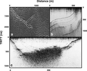
Our error analysis assumes that the processing steps satisfy at least the following requirements: (1) the time origin of the traces has been properly set for example by subtracting the propagation time between antennae centres to the first break of the direct wave; (2) normal moveout (NMO) correction has been applied before migration, to transform the common offset profiles into their respective zero-offset profiles (Yilmaz, Reference Yilmaz2001); (3) migration has been employed to restore shapes and slopes to their real values (Yilmaz, Reference Yilmaz2001), using the best available RWV; (4) ice thickness has only been picked where the bed is clearly identified in the radargrams (Fig. 2 shows examples of some situations where wrong picking might produce large errors, difficult to estimate) and (5) picking has been done at the maxima of the signal envelope (Nye and Berry, Reference Nye and Berry1974), for example by using the Hilbert transform (e.g. Taner and others, Reference Taner, Koehler and Sheriff1979; Moore and Grinsted, Reference Moore and Grinsted2006), which results in small picking errors on the order of the sampling period (e.g. Navarro and others, Reference Navarro2014).
Examples of radargrams showing difficulties in recognizing the bed reflection, taken from radargrams of Hurd Glacier, Livingston Island, Antarctica: (a) several possible bedrock reflections. (b) Internal ash layers of volcanic origin could be misinterpreted as bedrock. This is quite likely to happen if the bed reflection is not captured within the recording time window. (c) Bed reflection is hidden by strong scattering, probably due to water inclusions in the temperate ice layer.
Under such assumptions, the ice thickness H can be computed as
 $$H = \displaystyle{{c\;\tau} \over 2}$$
where c is the RWV in the medium and τ is the NMO-corrected TWTT. As the profiling offset (distance between antenna centres) is usually much smaller than the ice thickness, the NMO correction will typically affect only the shallowest parts of the profiles. Thus, the use of a flat reflector NMO correction should be sufficient (Dix, Reference Dix1955; Yilmaz, Reference Yilmaz2001):
 $$\tau = \sqrt {\tau _{\rm r}^2 - \left( {\displaystyle{d \over c}} \right)^2}, $$
where τ r is the recorded TWTT elapsed from the 0-time sample to the time sample picked for the bed reflection and d is the distance between transmitting and receiving antenna centres. If the offset is small compared with the ice thickness, this correction could be disregarded (compare e.g. corrections of ~15% if H = 2d, 1% if H = 7d and 0.1% if H = 20d).
The errors in RWV and in τ can be treated as independent (e.g. Navarro and Eisen, Reference Navarro, Eisen, Pellikka and Rees2010). Therefore, applying error propagation (e.g. Bevington and Robinson, Reference Bevington and Robinson2003) to Eqn (3) we get
 $$\varepsilon _{{H}\,{\rm GPR}} = \displaystyle{1 \over 2}\sqrt {\tau ^2 \varepsilon _{c}^2 + c^2 \varepsilon _\tau ^2},$$
where ε denotes the error in the variable indicated by the subscript.
3.1.1. Error in RWV
RWV varies from accumulation to ablation zones, mainly depending on the presence and characteristics (thickness, density, water/air content) of snow, firn and cold/temperate ice layers. The RWV relevant for a radar trace with picked bed reflection is the constant of proportionality to transform half the TWTT of the processed zero-offset profile into depth. Let us call it column-integrated RWV.
Since RWV is point dependent, ideally a 2-D map of column-integrated RWV should be available. However, the use of a constant RWV for the whole set of profiles is common practice (e.g. Shean and Marchant, Reference Shean and Marchant2010; Engel and others, Reference Engel, Nývlt and Láska2012; Singh and others, Reference Singh, Rathore, Bahuguna, Ramnathan and Ajai2012), although it can lead to locally biased estimations of ice thickness (e.g. overestimations in the ablation zone and underestimations in the accumulation zone, because of the presence of a firn layer in the latter). A potential solution could be using several discrete values of RWV for different profiles (using more precise RWV estimates for each one), but this introduces the alternative problem that then ice-thickness discontinuities may be introduced at crossover points, thus generating interpolation artifacts. A frequent improvement is implemented by adding a firn correction, proportional to a parameter quantifying the effect of firn (e.g. the snow-firn thickness or the elevation). This, however, requires that such a parameter has been estimated a priori from other available data or physical assumptions (e.g. Dowdeswell and Evans, Reference Dowdeswell and Evans2004; Rückamp and Blindow, Reference Rückamp and Blindow2012).
The value of RWV used is sometimes obtained by means of a common mid-point (CMP) measurement (e.g. Macheret and others, Reference Macheret, Moskalevsky and Vasilenko1993), or, more often, assigned a typical value considering the hydrothermal structure of the glacier, its location, the season of the radar campaign and the availability of neighbouring CMP measurements. Barrett and others (Reference Barrett, Murray and Clark2007) found that RWV obtained by CMP have errors between 0.2 and 3.5%, depending on the quality of the technique applied. However, CMP measures local values of RWV, which can differ from the average RWV used for time-to-thickness conversion of the set of radar profiles. For instance, Navarro and others (Reference Navarro2014), working on Hansbreen, a tidewater polythermal glacier in Svalbard, estimated a best fitting single RWV for the whole flowline, which differed from locally-measured RWVs (Jania and others, Reference Jania2005) by amounts between −2.3 and 2.3%. Following Bradford and others (Reference Bradford, Nichols, Mikesell and Harper2009), vertical profiles of RWV could be generated by means of multi-offset techniques, thus substantially improving the horizontal 2-D map of column-integrated RWV that we are assuming in this study. Using such techniques, they reduce the velocity uncertainty to <2%.
The assessment of the uncertainty in RWV (ε c in Eqn (5)) is based on experience. Since the correct RWV for each trace is a column-integrated value, its horizontal variability along the profile is not as large as that between the various englacial media (e.g. snow, firn, ice, or water) sampled along the profile (e.g. Jania and others, Reference Jania2005; Navarro and others, Reference Navarro2009). From the above discussion, uncertainties in RWV could be expected to lie between ~ 1 and 5% (i.e. ±1.7 to ±8.4 m µs−1). To select a particular value within this range, we suggest estimating the possible span of variability of column-integrated RWVs in the zone (either based on experience or using RWV measurements). The central RWV value of this range could be taken as RWV for the zone, and half the range used as the error in RWV. In our experience, 2% (~ ±3.4 m µs−1) is a proper choice of error in RWV when RWV is locally adapted (e.g. a 2-D map of RWV is available), while in cases using a single RWV for both accumulation and ablation zones, larger errors, up to 5% (±8.4 m µs−1), must be assumed.
3.1.2. Error in τ
The error in τ, or ‘timing error’, ε τ , is a measure of how precisely the reflection instant can be determined in a GPR record. Its contribution to the overall ice-thickness error is closely related to the concept of radar ‘resolution’. The GPR's range resolution (often termed as vertical resolution since most radar energy travels in the downward direction) is more relevant to our study than cross-range (or horizontal) resolution, even if the latter has an impact on the quality and representativeness of the GPR measurements. In Appendix A we discuss both range and cross-range resolutions.
We consider the vertical resolution, conservatively evaluated, as an estimate of ε τ . Therefore, we take ε τ = 1/f, which in terms of thickness is equivalent to λ/2. This implies for example ε τ = 50 ns for f = 20 MHz, or ε τ = 5 ns for f = 200 MHz. Assuming a RWV of 168 m µs−1, this is equivalent to 4.2 m for a 20 MHz radar, or 0.42 m for a 200 MHz radar.
Digital sampling in GPR recording systems also introduces an error in τ. However, the sampling period is usually much smaller than the vertical resolution of the wave in the medium (e.g. typical sampling –digitalization– periods of GPR systems are <0.5 ns for a 200 MHz GPR and <5 ns for a 20 MHz GPR, much smaller than the corresponding inverse of the central frequency, 5 and 50 ns respectively). Consequently, in general the sampling error can be neglected.
Another error in τ, which can be important, occurs when the reflection of the wave is not received from the nadir but from for example a lateral wall (off-nadir reflection, or out-of-plane reflection). Ground-based GPR measurements on valley glaciers often present this problem at profiles close and parallel to the glacier side walls. Airborne GPR measurements could also be affected by clutter from lateral mountains or other surfaces. Navarro and Eisen (Reference Navarro, Eisen, Pellikka and Rees2010) present some recommendations on fieldwork practices, regarding radar antennae layout and direction of profiling, aimed to minimize some of these errors. For ground-based measurements of valley glaciers, off-nadir reflections generate thicknesses smaller than the real ones, thus becoming a negative bias. Although it is a common practice to migrate these radar profiles, 2-D migration only restores slopes in the direction of profiling (migration is often not required in ice sheets, since bed slopes are small). Transversal slopes are not corrected, unless 3-D migration is applied. For instance, Moran and others’ (Reference Moran, Greenfield, Arcone and Delaney2000) results for 3-D processing over a small zone (100 m × 340 m) of the Gulkana Glacier, Alaska, show that 3-D migration restores thicknesses of the sloped-bed zones in their experiment area, increasing the thickness by up to 35% compared with the non-migrated radargrams, and up to 15% compared with the 2-D-migrated radargrams. However, it is unusual in glaciology to have a network of profiles dense enough to allow for 3-D processing and migration; there are only very few examples: Walford and others (Reference Walford, Kennett and Holmlund1986), Fisher and others (Reference Fisher1989), Welch and others (Reference Welch, Pfeffer, Harper and Humphrey1998) or Murray and Booth (Reference Murray and Booth2010). The latter authors discarded the 3-D migration of their 0.75 m spaced profiles, to avoid spatial aliasing, using 100 and 200 MHz GPR. Owing to the large error (negative local bias) that could be implied by the off-nadir reflections, every dataset that could potentially be affected by this error source should either be corrected (e.g. 3-D migrated or bias corrected) or discarded. In this study we assume that no measurements with such errors are being used. If an estimate of the error due to the lack of 3-D migration were available, it should be combined with the above estimate of ε τ computing the square root of their quadratic sum, since both errors are independent.
Another possible error in τ is the interpretation error that could be incurred when selecting the sample of the trace corresponding to the bed reflection (picking). The detection of the bed reflection can be done either manually or using automatic or semiautomatic algorithms, which are successfully used nowadays (e.g. MacGregor and others, Reference MacGregor2015). However, large errors can be introduced because bed reflections could easily be misinterpreted (Fig. 2 shows some examples). In such cases, the error cannot be estimated, though it could be very large. To avoid this situation, to facilitate an error estimate, and to avoid picking in the traces where there are doubts about where the bed reflection is located, we recommend an expert review of the picking results. Accordingly, this source of error is not taken into account in this study.
3.1.3. Relation between the error in RWV and the error in τ
Eqn (5) can be rewritten:
 $$\varepsilon _{{H}\,{\rm GPR}} = \sqrt {\varepsilon _{{Hc}}^2 + \varepsilon _{{H\tau}} ^2},$$
where ε Hc = ε c τ/2 and ε Hτ = c ε τ /2 are the components of the error in thickness due to the error in RWV and to the error in τ respectively.
Taking into account the measured ice thickness and the GPR frequency, it is possible to compare the effects of both errors, and to determine in which cases one can be neglected compared with the other. Figure 3 illustrates an example.
Error in GPR ice-thickness measurement and its components as given by Eqn (6) for ice-thickness measurements up to 1000 m, recorded using a 20 MHz GPR and assuming a RWV of 168 m µs−1, ε c = 0.02c and ε τ = 1/f. The green curve shows the 90% of ε HGPR.

ε Hc increases linearly with the ice thickness, while ε Hτ does not depend on the ice thickness. Considering as negligible any influence of ε Hτ on ε HGPR below for example 10%, the thickness h 0 beyond which the influence is negligible, compared with ε Hc can be obtained using ε H GPR = ε Hc /0.9. Assuming c = 168 m µs−1, ε c = 0.02c and ε τ = 1/f, we get h 0 = 8672/f (in m, if f is given in MHz). At deeper thicknesses the approximation ε H GPR = ε c τ/2 can be used. For instance, we can neglect ε Hτ for ice thickness larger than ~43 m if a 200 MHz GPR is used, or larger than ~434 m for a 20 MHz GPR (Fig. 3 illustrates this latter case).
3.2. Positioning-related ice-thickness error
The location of each GPR data point is affected by a horizontal-positioning error, ε
xy
, which, for a varying ice thickness, leads to a positioning-related ice-thickness error in the data, ε
H
xy
. We characterize the uncertainty in position, ε
xy
, by its values ε
 $_{xy\,\parallel} $
and ε
xy ⊥ along and across the profiling direction respectively. To estimate ε
H
xy
we study the variability of ice thickness along each axis, within the corresponding distances from the data point (ε
$_{xy\,\parallel} $
and ε
xy ⊥ along and across the profiling direction respectively. To estimate ε
H
xy
we study the variability of ice thickness along each axis, within the corresponding distances from the data point (ε
 $ _{xy\,\parallel} $
and ε
xy ⊥). We evaluate the positioning-related ice-thickness error at the data point denoted with subscript i, ε
Hxy
i
, as
$ _{xy\,\parallel} $
and ε
xy ⊥). We evaluate the positioning-related ice-thickness error at the data point denoted with subscript i, ε
Hxy
i
, as
 $${\varepsilon} _{{H}xy_i} \, = \,\sqrt {{ \varepsilon} _{{H}xy\,\parallel _i} ^2 + {\varepsilon} _{{H}xy \bot _i} ^2}.$$
where
 ${\varepsilon} _{{H}xy\parallel _i} $
and
${\varepsilon} _{{H}xy\parallel _i} $
and
 ${\varepsilon} _{{H}xy \bot _i} $
are the estimates of thickness variability along each axis. These are evaluated as the maximum absolute value of the discrepancies in thickness found, along the corresponding axis, within a distance from the current data point smaller than the corresponding error in position. The discrepancies in thickness along the profiling direction are calculated using the ice-thickness data points, while those across the profile are best evaluated from a DEM of ice thickness.
${\varepsilon} _{{H}xy \bot _i} $
are the estimates of thickness variability along each axis. These are evaluated as the maximum absolute value of the discrepancies in thickness found, along the corresponding axis, within a distance from the current data point smaller than the corresponding error in position. The discrepancies in thickness along the profiling direction are calculated using the ice-thickness data points, while those across the profile are best evaluated from a DEM of ice thickness.
When the horizontal uncertainty ε xyi is constant in all directions (let us call it isotropic uncertainty), there is no need to split along two axes this error estimate. In this case, we estimate the positioning-related ice-thickness error as the maximum discrepancy found (absolute value) between the value at the data point and the neighbouring values within a circle of radius ε xyi , using a DEM of ice thickness.
3.2.1. Positioning error due to GPS uncertainty
GPS is nowadays the most commonly used technique for positioning. The horizontal error in a GPS position is isotropic, and takes the value of the horizontal accuracy of the GPS measurement, i.e.
 ${\varepsilon} _{xy\,\parallel} = {\varepsilon} _{xy\, \bot} $
. The latter could be neglected if trace positioning is obtained by differential GPS (dGPS), due to its accuracy on the order of centimetres. However, when using SPS (GPS Standard Positioning Service) this error should be taken into account.
${\varepsilon} _{xy\,\parallel} = {\varepsilon} _{xy\, \bot} $
. The latter could be neglected if trace positioning is obtained by differential GPS (dGPS), due to its accuracy on the order of centimetres. However, when using SPS (GPS Standard Positioning Service) this error should be taken into account.
A substantial improvement in the use of GPS for civilian applications occurred in May 2000, when the Department of Defense of the USA deactivated the GPS Selective Availability (SA) feature. SA was an intentional degradation of civilian GPS accuracy, implemented on a global basis through the GPS satellites. Before May 2000, as a result of the SA, position readings using SPS could be incorrect by up to 100 m. After the SA deactivation, SPS accuracy improved tenfold, and nowadays the typical accuracy of SPS is ~5 m. More information on SPS accuracy and its evolution can be found for example in the Official U.S. Government information about the GPS and related topics, (http://www.gps.gov).
3.2.2. Trace-positioning error due to GPR movement
It is common practice in GPR profiling to obtain trace positions automatically by GPS. Since GPR travels at a certain velocity v while profiling, the horizontal-positioning error of each trace, ε xy , could be split into two independent errors: the GPS accuracy, ε xy GPS, and the displacement of the GPR during the time interval between the GPS-coordinates update (or refreshing) and the trace recording, ε Δxy . The uncertainty of the former is isotropic, while that of the latter is in the direction of profiling. Therefore, associated with each trace there is an ellipse of uncertainty whose axes can be obtained by the combination of both independent error components, orthogonal to each other. The uncertainty component in the orthogonal direction is just ε xy ⊥ = ε xy GPS, while that in the travel direction results from the combination of both independent components, through their squared quadratic summation,
 $${\varepsilon} _{xy\,\parallel} = \sqrt {{\varepsilon} _{xy\,{\rm GPS}}^2 + {\varepsilon} _{\Delta xy}^2},$$
where ε Δxy depends on v, on the time step between subsequent traces, T GPR, and on the update period of the GPS data, T GPS. The magnitude of the displacement is given by
 $${\varepsilon} _{\Delta xy} = v\;{\varepsilon} _{T},$$
where ε T characterizes the timing differences due to lack of synchronization between the GPS-coordinates update and the trace recording. In practice, it could be estimated as the minimum of T GPR and T GPS, although its value depends on how the coordinates have been assigned to traces. A detailed discussion about this subject can be found in Appendix B.
In some cases, especially when using archived data, GPR-prospecting metadata may not be available, preventing the use of some of the above equations. In such cases, some standard values could be used. For instance, typical values for v could be 10–30 km h−1 when profiling by snowmobile, 1–4 km h−1 when prospecting by foot, 70–100 km h−1 when by helicopter and larger values if by fixed-wing aircraft. T GPR could be deducted from the assumed profiling velocity and the distance between recorded traces. Finally, T GPS is often 1 s when using SPS (though it could be up to 5 s, depending on the receiver), while when using differential GPS it is an adjustable parameter, with common values between 0.1 and 1 s.
If there are insufficient fieldwork metadata, Eqn (8) could be isotropically extended, thus providing a simple and conservative estimate of the radius of uncertainty around the trace position, ε xy .
Figure 4 shows the error in thickness corresponding to a given error in positioning (whatever the source of error in positioning is) and a given bedrock slope. In combination with Table 1, which estimates the trace positioning error due to GPR movement, it is straightforward to estimate the error in ice thickness due to GPR movement. For instance, in airborne profiling from helicopter, travelling at 100 km h−1, recording one trace per second and with GPS position refreshed also every second, Table 1 gives an error in position of 27.8 m. If the bedrock slopes 30° in the direction of movement, we then find from Figure 4 that the error in ice thickness is >16 m, no matter the accuracy of the GPS used.
Error in ice thickness, ε H x y (m), for a given error in position, ε xy , and a given bed slope with angle θ.

Trace-positioning errors, ε Δxy (m), calculated using Eqn (9) for different combinations of convoy velocity and time uncertainty, ε T (Appendix B)
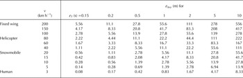
Figure 4, in combination with Table 1, is a useful tool to estimate the positioning-related error for a given combination of profiling parameters (velocity of the convoy, bed slope, refreshing period of the GPS and triggering interval of the GPR). They help the GPR operator to select a priori proper settings of parameters in GPR profiling, aimed to minimize the trace-positioning error due to GPR movement and the related error in thickness. Also, a posteriori, they help to decide whether these errors are relevant or should instead be neglected.
3.2.3. Trace-positioning error due to improper position of the GPS antenna
If the GPS antenna is not installed at the midpoint of the GPR antenna centres, the trace position will be affected by a bias vector. This vector has a constant modulus and its direction changes forming a constant angle with the profiling direction. Thus, it is specific for each trace, and should either be corrected or accounted for as an error.
A simpler but less accurate approach is to treat it as an isotropic uncertainty, applying the same error to all traces. The distance between the GPS antenna and the midpoint of the GPR antenna centres will be used as the error radius. This distance must be combined in square summation both with
 $\varepsilon _{xy\,\parallel} $
and with ε
xy ⊥ separately.
$\varepsilon _{xy\,\parallel} $
and with ε
xy ⊥ separately.
3.2.4. Trace-positioning error when positioning data for each trace are not available
In glaciological applications, GPR triggering is often controlled by time, though sometimes by odometer. GPS trace positioning can be used in both cases, recording the coordinates and sufficient timing information to estimate the position accuracy. However, GPR traces are not always positioned by GPS, especially when using old archived data. Sometimes just the profile endpoints are positioned (e.g. by GPS), and evenly spaced trace positions, along the straight line joining both endpoints, are assumed, no matter whether the triggering is performed by odometer or by time (assuming, in the latter case, a constant GPR profiling velocity). In these cases, Eqn (7) should be used to estimate
 $\varepsilon _{{H}xy_i} $
, though different horizontal accuracies, ε
xyi
, for each trace of the profile should be used, because of their expected different horizontal deviations from the straight line (Fig. 5).
$\varepsilon _{{H}xy_i} $
, though different horizontal accuracies, ε
xyi
, for each trace of the profile should be used, because of their expected different horizontal deviations from the straight line (Fig. 5).
The path followed by the GPR while profiling is shown in blue. The dashed straight line is that joining the profile endpoints. D represents the distance between the real position and the straight line, for a certain trace. The uncertainty at the endpoints is represented by both orange circles. The orange curves are parabolas with maximum horizontal displacement at the centre of the profile equal to 5% and 15% of the distance between endpoints plus the uncertainty of the endpoint positioning.
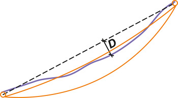
Depending on the profile length, this horizontal deviation could be much larger than the current typical SPS uncertainty of 5 m. To evaluate the deviation, any information about how straight the profile was would be useful, for example a GPS track externally recorded while profiling (e.g. by the snow mobile navigation GPS). In the absence of other information it can be assumed that the horizontal deviation from the straight line has a parabolic shape, with a maximum value at the centre of the profile of ~5–15% of the distance between endpoints, added to the uncertainty of the endpoints positioning. The resulting value at each trace can then be used as an estimate of ε xyi .
Other considerations regarding the fieldwork practices should also be kept in mind. For instance, one should be aware of a possible shift between the measured positioning of the profile endpoints and the real position of the first and last traces recorded by the GPR. This would produce a bias in the trace coordinates, increasing their uncertainty. In the absence of field information about this offset, no bias should be considered, but it would be reasonable to increase the positioning uncertainty of the profile endpoints.
The expected variability of the GPR profiling velocity (or, equivalently, the non-uniform behavior of the odometer due for example to varying snow surface conditions) also produces an added uncertainty in the trace positioning. However, since the deviation of the trace position from the straight line has been conservatively assumed as an isotropically-extended ratio of uncertainty, the mentioned errors can be considered as implicitly included in our trace-positioning error estimate.
4. CASE STUDIES
Following, the above-discussed error estimate techniques are applied to two case studies. The first is a real case, while the second is simulated and shows the errors that would appear in the first case if the GPR profiling were done using different parameters.
4.1. Werenskioldbreen
For this purpose we have chosen the GPR ice-thickness measurements carried out in April 2008 on Werenskioldbreen (see Acknowledgements), a land-terminating polythermal glacier on Southern Spitsbergen, Svalbard (Fig. 6) (Navarro and others, Reference Navarro2014).
Location of Werenskioldbreen in Svalbard and layout of GPR profiles showing the spatial distribution of the available GPR data. Black sections of the profiles represent data from profiles parallel and close to large lateral slopes, which have been removed from the working dataset due to their likely large and difficult-to-evaluate error. The colour scale shows the ice thickness H.

The GPR data were collected using a 25 MHz Ramac/GPR (Malå Geoscience, Sweden). The distribution of the GPR data over the glacier surface is uneven (Fig. 6); it is dense along the profiles, but there are large areas devoid of data between some radar profiles. The migration algorithm applied was Stolt F-K (e.g. Yilmaz, Reference Yilmaz2001). We used a 2-D map of RWV for time-to-depth conversion. It assumes an RWV of 166 m µs−1 for the ablation zone, which linearly increases from the ELA, set at 400 m a.s.l., to reach 170 m µs−1 at the maximum elevation of the glacier (~560 m a.s.l.). The ELA choice is based on the study by Ignatiuk and others (Reference Ignatiuk, Piechota, Ciepły and Luks2014). Picking of bedrock reflections was done taking into account the recommendations given in Section 3.1.2. We performed a crossover analysis that revealed discrepancies at the intersecting points on the order of the vertical resolution of the GPR. This shows the consistency of the ice-thickness data, though cannot be used as an indication of the errors involved.
For some profiles we expect to have large ice-thickness errors, as they are close and parallel to steep lateral slopes, which generate off-nadir reflections that cannot be corrected by 2-D migration. To estimate these slopes, we built a first approach to an ice-thickness DEM using the whole dataset. Details of this DEM are described in the case study of Lapazaran and others (Reference Lapazaran, Otero, Martín-Español and Navarro2016; this issue (Paper II)). We then analysed which profiles or part of profiles were close and parallel to steep slopes, removing them from the dataset (black profile sections in Fig. 6).
We calculated the errors in the GPR-retrieved values of ice thickness,
 $\varepsilon _{{H}\,{\rm GPR}_i} $
, shown in Figure 7a, using Eqn (5). For such calculations, we considered a relative error in RWV of 2%. We took ε
τ
as 1/f, which corresponds to a vertical resolution of λ/2 (3.32–3.40 m respectively, at the lower and upper parts of the glacier). This produced values of
$\varepsilon _{{H}\,{\rm GPR}_i} $
, shown in Figure 7a, using Eqn (5). For such calculations, we considered a relative error in RWV of 2%. We took ε
τ
as 1/f, which corresponds to a vertical resolution of λ/2 (3.32–3.40 m respectively, at the lower and upper parts of the glacier). This produced values of
 $\varepsilon _{{H}\,{\rm GPR}_i} $
between 3.32 and 6.61 m, with a mean value of 4.48 m and a standard deviation of 0.83 m.
$\varepsilon _{{H}\,{\rm GPR}_i} $
between 3.32 and 6.61 m, with a mean value of 4.48 m and a standard deviation of 0.83 m.
(a) Error in the value of the ice thickness for each point in the GPR dataset,
 $\varepsilon _{{H}\,{\rm GPR}_i} $
. (b) Error in ice thickness due to the horizontal-positioning uncertainty,
$\varepsilon _{{H}\,{\rm GPR}_i} $
. (b) Error in ice thickness due to the horizontal-positioning uncertainty,
 $\varepsilon _{{H}xy_i} $
. (c) Error in thickness of the data,
$\varepsilon _{{H}xy_i} $
. (c) Error in thickness of the data,
 $\varepsilon _{H{\rm data}_i} $
, resulting from combining the errors shown in (a) and (b) using Eqn (2).
$\varepsilon _{H{\rm data}_i} $
, resulting from combining the errors shown in (a) and (b) using Eqn (2).

Figure 7b shows the positioning-related ice-thickness error at each GPR measurement point,
 $\varepsilon _{{H}xy_i} $
, estimated using Eqns (7)–(9). Taking into account that the radar traces were positioned using post-processed differential GPS data, we considered a radius of horizontal uncertainty of ε
xy
= 0.05 m, so this error can be neglected. The dGPS refreshing period was T
GPS = 1 s, the GPR travelling speed was v ~ 11 km h−1, and the time interval between traces was T
GPR = 0.5 s, thus producing on average one trace every ~1.5 m, though a new GPS position only every ~3 m (case b in Appendix B). Since the distances between profiles were much larger than the distances between traces, the positions were not interpolated (case bI in Appendix B). Instead, the data were decimated, keeping only traces with updated GPS position (case bII, in Appendix B). As no bias correction was applied to shift the trace coordinates in the direction of profiling, we characterized ε
T
by 0.5 s (Table 3 in Appendix B). Then, according to Eqns (9) and (8),
$\varepsilon _{{H}xy_i} $
, estimated using Eqns (7)–(9). Taking into account that the radar traces were positioned using post-processed differential GPS data, we considered a radius of horizontal uncertainty of ε
xy
= 0.05 m, so this error can be neglected. The dGPS refreshing period was T
GPS = 1 s, the GPR travelling speed was v ~ 11 km h−1, and the time interval between traces was T
GPR = 0.5 s, thus producing on average one trace every ~1.5 m, though a new GPS position only every ~3 m (case b in Appendix B). Since the distances between profiles were much larger than the distances between traces, the positions were not interpolated (case bI in Appendix B). Instead, the data were decimated, keeping only traces with updated GPS position (case bII, in Appendix B). As no bias correction was applied to shift the trace coordinates in the direction of profiling, we characterized ε
T
by 0.5 s (Table 3 in Appendix B). Then, according to Eqns (9) and (8),
 $\varepsilon _{\Delta xy} = \varepsilon _{xy\,\parallel} = 1.5\,{\rm m}$
along the profiling directions. These uncertainties in position generate ice-thickness errors up to 3.08 m, with a mean value of 0.56 m and a standard deviation of 0.43 m.
$\varepsilon _{\Delta xy} = \varepsilon _{xy\,\parallel} = 1.5\,{\rm m}$
along the profiling directions. These uncertainties in position generate ice-thickness errors up to 3.08 m, with a mean value of 0.56 m and a standard deviation of 0.43 m.
Figure 7c shows the errors in ice thickness of the data,
 $\varepsilon _{H{\rm data}_i} $
, obtained using Eqn (2), as a combination of the errors in ice-thickness value obtained from the GPR data,
$\varepsilon _{H{\rm data}_i} $
, obtained using Eqn (2), as a combination of the errors in ice-thickness value obtained from the GPR data,
 $\varepsilon_{{H}\,{\rm GPR}_i} $
(Fig. 7a), and the errors in thickness due to position uncertainty,
$\varepsilon_{{H}\,{\rm GPR}_i} $
(Fig. 7a), and the errors in thickness due to position uncertainty,
 $\varepsilon _{{H}xy_i} $
(Fig. 7b). These final errors range between 3.32 m (vertical resolution) and 6.78 m, with a mean value of 4.53 m and a standard deviation of 0.83 m.
$\varepsilon _{{H}xy_i} $
(Fig. 7b). These final errors range between 3.32 m (vertical resolution) and 6.78 m, with a mean value of 4.53 m and a standard deviation of 0.83 m.
We note that both error components are spatially distributed in a non-uniform way and that none of them is negligible, compared with the other. Large values of
 $\varepsilon _{{H}\,{\rm GPR}_i} $
are associated with large ice thicknesses. There is a trend towards large values of
$\varepsilon _{{H}\,{\rm GPR}_i} $
are associated with large ice thicknesses. There is a trend towards large values of
 $\varepsilon_{{H}xy_i} $
in areas of large gradients of ice thickness, for instance in areas of steeply sloped bed, where ice thickness is usually small. This illustrates that both error components have to be taken into account to obtain reliable ice-thickness error estimates.
$\varepsilon_{{H}xy_i} $
in areas of large gradients of ice thickness, for instance in areas of steeply sloped bed, where ice thickness is usually small. This illustrates that both error components have to be taken into account to obtain reliable ice-thickness error estimates.
4.2. Helicopter simulation on Werenskioldbreen
4.2.1. Bias in position not corrected
This case study is a simulation based on the previous case. Here we estimate the errors in thickness derived from the uncertainty in position based on a different set of profiling parameters. For the simulation we are considering that the data were collected traveling with a constant velocity of 100 km h−1 (e.g. by helicopter), at a rate of one trace s−1, and using a dGPS (5 cm accuracy), with position refreshed every 1 s. This implies an assumed distance between traces of 27.8 m.
We generated a new dataset for this case study, taking one datum every ~27.8 m from the original dataset of Werenskioldbreen. The errors in the GPR-retrieved values of ice thickness,
 $\varepsilon _{{H}\,{\rm GPR}_i} $
, are thus coincident with those of the previous case study. However, since it is a subset of the original dataset, its statistics are different: the values of
$\varepsilon _{{H}\,{\rm GPR}_i} $
, are thus coincident with those of the previous case study. However, since it is a subset of the original dataset, its statistics are different: the values of
 $\varepsilon _{{H}\,{\rm GPR}_i} $
range from 3.32 to 6.56 m, with a mean value of 4.53 m and a standard deviation of 0.84 m.
$\varepsilon _{{H}\,{\rm GPR}_i} $
range from 3.32 to 6.56 m, with a mean value of 4.53 m and a standard deviation of 0.84 m.
As
 $\varepsilon _{T} = \min \left( {T_{{\rm GPS}}, T_{{\rm GPR}}} \right)$
(Appendix B), and T
GPR = T
GPS = 1 s, we get ε
T
= 1 s. Using this value in Eqn (9) or Table 1 with v = 100 km h−1, we obtain ε
Δxy
= 27.8 m. Following the same rationale as in the previous case study, we can neglect the uncertainty of 5 cm in the transverse direction.
$\varepsilon _{T} = \min \left( {T_{{\rm GPS}}, T_{{\rm GPR}}} \right)$
(Appendix B), and T
GPR = T
GPS = 1 s, we get ε
T
= 1 s. Using this value in Eqn (9) or Table 1 with v = 100 km h−1, we obtain ε
Δxy
= 27.8 m. Following the same rationale as in the previous case study, we can neglect the uncertainty of 5 cm in the transverse direction.
In Figure 8a we show the derived errors in thickness. The uncertainties in position generate ice-thickness errors up to 22.69 m, with a mean value of 5.03 m and a standard deviation of 3.94 m.
For case study 4.2.1: (a) Error in ice thickness due to the horizontal-positioning uncertainty,
 $\varepsilon _{{H}xy_i} $
. (b) Error in thickness of the data,
$\varepsilon _{{H}xy_i} $
. (b) Error in thickness of the data,
 $\varepsilon _{H{\rm data}_i} $
. The scale is coincident with that of Figure 7 in the overlapping range.
$\varepsilon _{H{\rm data}_i} $
. The scale is coincident with that of Figure 7 in the overlapping range.
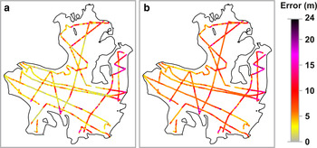
Figure 8b shows the errors in ice thickness of the data,
 $\varepsilon _{H{\rm data}_i} $
, which range between 3.42 m (vertical resolution) and 23.18 m, with a mean value of 7.22 m and a standard deviation of 3.15 m. They were obtained using Eqn (2), as a combination of the errors in the value of ice-thickness obtained from the GPR data,
$\varepsilon _{H{\rm data}_i} $
, which range between 3.42 m (vertical resolution) and 23.18 m, with a mean value of 7.22 m and a standard deviation of 3.15 m. They were obtained using Eqn (2), as a combination of the errors in the value of ice-thickness obtained from the GPR data,
 $\varepsilon _{{H}\,{\rm GPR}_i} $
(same as in Fig. 7a), and the errors in thickness due to position uncertainty,
$\varepsilon _{{H}\,{\rm GPR}_i} $
(same as in Fig. 7a), and the errors in thickness due to position uncertainty,
 $\varepsilon _{{H}xy_i} $
(Fig. 8a). We conclude that the errors in thickness derived from the uncertainty in position are dominant in this case in large portions of the glacier.
$\varepsilon _{{H}xy_i} $
(Fig. 8a). We conclude that the errors in thickness derived from the uncertainty in position are dominant in this case in large portions of the glacier.
4.2.2. Correcting bias in position
Based on the same case study, we now apply the correction of the bias in position (aI, bIII or bIV in Appendix B, since T GPR = T GPS), thus reducing the error in position of the corrected traces.
Since v = 100 km h−1, i.e. 27.8 m s−1, and ε T = 1 s, the bias corresponds to the displacement of 0.5 s at this velocity, i.e. 13.9 m. Thus, a new position is assigned to each trace, obtained displacing its coordinates 13.9 m forward in the profiling direction, as defined by the vector joining the positions of the current and next trace.
The uncertainty in timing of data acquisition is now reduced to
 $1/\sqrt {12} $
s, which in terms of space, at the given profiling velocity, is
$1/\sqrt {12} $
s, which in terms of space, at the given profiling velocity, is
 ${\varepsilon} _{\Delta xy} = 27.8/\sqrt {12} = 8.0\,\,\rm m$
.
${\varepsilon} _{\Delta xy} = 27.8/\sqrt {12} = 8.0\,\,\rm m$
.
In Figure 9a we show the corresponding errors in thickness. The uncertainties in position generate ice-thickness errors up to 6.55 m, with a mean value of 1.44 m and a standard deviation of 1.12 m.
For case study 4.2.2: (a) Error in ice thickness due to the horizontal-positioning uncertainty, ε Hxy i . (b) Error in thickness of the data, ε Hdata i . The scale is coincident with that of Figure 7 in the overlapping range.

Figure 9b shows the errors in ice thickness of the data,
 $\varepsilon _{H{\rm data}_i} $
, which range between 3.34 and 8.09 m, with a mean value of 4.87 m and a standard deviation of 0.92 m. They were obtained using Eqn (2), as combination of the errors in the value of ice thickness obtained from the GPR data,
$\varepsilon _{H{\rm data}_i} $
, which range between 3.34 and 8.09 m, with a mean value of 4.87 m and a standard deviation of 0.92 m. They were obtained using Eqn (2), as combination of the errors in the value of ice thickness obtained from the GPR data,
 $\varepsilon _{{H}\,{\rm GPR}_i} $
(they have not changed since Fig. 7a), and the errors in thickness due to position uncertainty,
$\varepsilon _{{H}\,{\rm GPR}_i} $
(they have not changed since Fig. 7a), and the errors in thickness due to position uncertainty,
 $\varepsilon _{{H}xy_i} $
(Fig. 9a). As we see, applying the bias correction has resulted in a significant reduction of the error in thickness.
$\varepsilon _{{H}xy_i} $
(Fig. 9a). As we see, applying the bias correction has resulted in a significant reduction of the error in thickness.
5. CONCLUSIONS
We have developed a systematic methodology to estimate the error in ice-thickness measurements from GPR data. The error is split into various independent components, which can be estimated separately, thus allowing the study of their different effects.
We showed a comparison of the effects of the error in RWV versus the error in TWTT, which allows to easily determine when one of these errors can be neglected, compared with the other.
We present a novel method to analyse the uncertainty in horizontal positioning of the GPR measurement points due to the GPR movement during profiling, which depends on (1) the profiling velocity, (2) the GPS refreshing period and (3) the GPR triggering period. This error is especially relevant for airborne profiling.
We also presented a novel method to estimate the effects, in terms of ice-thickness error, of the uncertainty in horizontal positioning of the GPR measurement points. These effects are estimated based on the local variability of the ice-thickness dataset and of a DEM of ice thickness built from it.
Figure 4, together with Table 1, are useful to roughly estimate the positioning-related error for a given combination of profiling parameters such as velocity of the measurement vehicle, bed slope, refreshing period of the GPS and triggering interval of the GPR. They allow selecting a priori optimal settings of parameters in GPR profiling, in the sense of minimizing the trace-positioning error due to GPR movement and its related error in thickness. Additionally, they help to calculate, a posteriori, the approximate magnitude of these errors, and decide whether they can be neglected or a more detailed error study is recommended.
All the above techniques were applied to a real case study (Werenskioldbreen, Svalbard) and to a simulated one, based on the former. An important conclusion was that the ice-thickness error due to the uncertainty in the horizontal positioning of the radar data, ignored in the literature, must be taken into account, since sometimes it can be the main source of error in ice thickness. This happened in our simulated case study, in which a profiling velocity typical of helicopter sounding (100 km h−1), and GPR triggering time and GPS refreshing period of 1 s, resulted in a positioning error of the radar traces of 27.8 m in the profiling direction, generating errors in thickness of 5.03 m in average, with a maximum value of 22.69 m, and a standard deviation of 3.94 m. These errors were dominant in large portions of the glacier, illustrating that the error in ice thickness due to the uncertainty in horizontal positioning of the radar data should not be overlooked. We also showed that correcting for the bias in position generated by movement of the GPR while profiling results in substantial reductions of the positioning error, and hence in its associated error in thickness.
ACKNOWLEDGEMENTS
We thank the scientific editor, Jo Jacka, and three anonymus reviewers for their valuable comments and suggestions that helped improving the quality of this paper. This research was supported by grants CTM2011-28980 and CTM2014-56473-R from the Spanish National Plan for R&D. We thank Jacek Jania and Mariusz Grabiec (Faculty of Earth Sciences, University of Silesia), and Dariusz Puczko (Institute of Geophysics, Polish Academy of Sciences) for making available the Werenskioldbreen GPR data.
APPENDIX A
RANGE AND CROSS-RANGE RESOLUTION
Since most radar energy travels in the downward direction, the GPR's range and cross-range resolutions are often termed as vertical and horizontal resolutions respectively. Hereafter there is a discussion about the resolution in pulsed radars.
CROSS-RANGE RESOLUTION OR HORIZONTAL RESOLUTION
The horizontal resolution of pulsed radar data depends on both the central frequency of the radar, f, and the measured ice thickness, H. It is usually characterized by the radius of the first Fresnel zone, defined as the zone of the reflecting surface that contributes to a single reflection (e.g. Robin and others, Reference Robin, Evans and Bailey1969; Yilmaz, Reference Yilmaz2001). It can be regarded as the size of the ‘footprint’ of the radar signal, thus providing an estimate of its horizontal resolution. The radius of the first Fresnel zone, r, can be obtained as
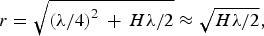 $$r = \sqrt {\left( {{\lambda / 4}} \right)^2 \, + \,{{H\lambda} / 2}} \approx \sqrt {{{H\lambda} / 2}}, $$
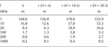
where λ = c/f is the dominant radar wavelength, with c the RWV. The first term within the root can in practice be neglected, as its contribution to r is <3% when the ice thickness is larger than the wavelength. Table 2 shows some examples of radius of the first Fresnel zone, obtained using its most complete expression in Eqn (A1), for different typical frequencies of GPR, at depths of 1, 10 and 20 wavelengths, assuming a RWV of 168 m µs−1.
Relationship between the radius of the first Fresnel zone and the wavelength
Although the horizontal resolution of a single trace is determined by the Fresnel radius, migration can improve the horizontal resolution along a profile. During migration, additional data of the adjacent traces are used, improving and shortening the Fresnel radius in the migration direction, parallel to the profile, to ~λ/2, regardless of the depth (Yilmaz, Reference Yilmaz2001, pp.1801, 1805; Welch and others, Reference Welch, Pfeffer, Harper and Humphrey1998). However, resolution in the direction perpendicular to the profile is not affected by 2-D migration. Therefore, the horizontal resolution of the radar is not uniform, if the profiles are not migrated, or anisotropic, if the profiles are migrated. 3-D migration should generate ice-thickness data with uniform and isotropic horizontal resolution, although it is not a common event in glaciology, as was discussed earlier.
RANGE RESOLUTION OR VERTICAL RESOLUTION
The reflections of a radar wave from two reflectors separated by a distance ∆d are received at two different times separated by a time interval ∆t (∆d = c ∆t/2, in zero-offset approximation and with c spatially uniform). The GPR vertical resolution indicates how close two reflectors may be vertically located so that they can still be distinguished by the radar. The vertical resolution can be evaluated either in the time or space domains, which are related through the RWV. We evaluate the vertical resolution in the time domain, since its independence with respect to the error in RWV simplifies the error calculation.
Pulsed radar resolution increases with the dominant (or central) frequency of the transmitted pulse, f, and decreases with the presence of noise. Resolution can be improved during the radargram processing as a result of deconvolution (e.g. Yilmaz, Reference Yilmaz2001). For a radar signal with wavelength λ (λ = c/f), Widess (Reference Widess1973) evaluated the vertical resolution in the space domain as being λ/8, which is equivalent in time to 1/4f (expressed as TWTT). However, his analysis was based on a simplified reflecting model in a homogeneous medium, in the absence of noise, far from reality. It is more common to evaluate the vertical resolution as λ/4 (1/2f in TWTT) (e.g. Yilmaz, Reference Yilmaz2001). However, real media are complex and the GPR wavelet is extended among several wavelengths in real radargrams, so that λ/4 is not always a realistic value (e.g. Reynolds, Reference Reynolds1997) and it may be preferable to use λ/2 (e.g. Hubbard and Glasser, Reference Hubbard and Glasser2005; Pérez-Gracia and others, Reference Pérez-Gracia, Di Capua, González-Drigo and Pujades2009; Navarro and Eisen, Reference Navarro, Eisen, Pellikka and Rees2010).
APPENDIX B
TRACE-POSITIONING ERROR IN A MOVING GPR USING GPS
Let us consider a GPR traveling under the conditions of validity of Eqn (8)
 $$\varepsilon _{xy\;\parallel} = \sqrt {\varepsilon _{xy\,{\rm GPS}}^2 + \varepsilon _{\Delta xy}^2}, $$
for which the uncertainty of ε xy GPS was isotropic, while that of ε Δxy was in the profiling direction. We aim to estimate the value of the latter.
We assume the most common case, i.e. that there is a GPS connected to the GPR, which automatically associates with each recorded trace the most recent coordinates obtained by the GPS. It is also assumed that, if any biases on the trace positions exist (e.g. due to installation of the GPS out from the midpoint of the GPR antennas), they have been corrected separately.
According to Eqn (9), ε Δxy = v ε T , where we recall that ε T represents the dispersion of the error random variable e T (time interval between GPS-position actualization and GPR-trace acquisition). When e T is a bias-free random variable, its standard deviation characterizes ε T .
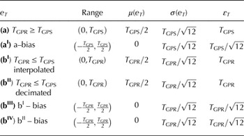
We consider two main cases: (a) the time step between traces is larger than that between GPS-coordinate updates, i.e. T GPR ≥ T GPS and (b) T GPR ≤ T GPS. In both cases, the sequence of trace-recording times is t 1, t 2,…, t i …, while the updates of GPS coordinates happen at times s 1, s 2, …, s k …. In case a, to each t i is assigned the value of the most recent s k obtained by the GPS, while in case b the same time s k is assigned to several t i (Fig. 10). In both cases, e T is simply the time interval between each s k and the corresponding t i , and takes values between 0 and T GPS.
The horizontal axis represents time, increasing from left to right. Orange dots show time instants of trace recording, while instants of GPS update are shown in blue. The blue arrows indicate which GPS-measured data are assigned to each GPR-recorded trace. The green arrows indicate which corrected coordinates are associated with the corresponding traces, both due to interpolation and to bias correction. Six cases are shown: Case (a): The period between traces is larger than the GPS-updating period, T GPR ≥ T GPS. Case (aI): The bias is added to the traces of case a. Case (b): T GPR ≤ T GPS. Case (bI): A correction is applied to case b, assigning interpolated coordinates to the traces with repeated coordinates. Case (bII): Traces from case b are decimated, preserving only those with updated GPS position. Case (bIII): A second correction is applied to case b, adding the bias to the traces of bI.
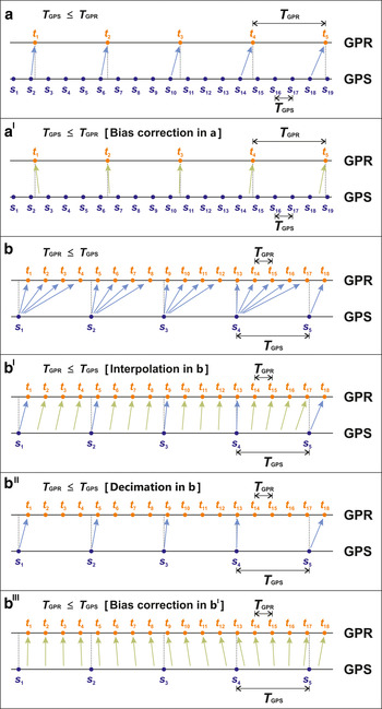
Since in case b several traces have repeated coordinates, the original GPR data cannot be used without previous manipulation. It is a common practice to interpolate the data between updated coordinates (case bI in Fig. 10). In such a case, assuming a constant speed during the period T GPS, the maximum value of e T is reduced to T GPR. Alternatively, if T GPR is too small, traces in case b can be decimated instead of interpolating their positions, keeping only the traces with updated coordinates (case bII in Fig. 10), i.e. as if in Figure 10b only the traces t 1, t 5, t 9, t 13, t 18, … were kept. Consequently, e T takes values between 0 and T GPR. As a result, in each of the cases a, bI and bII,
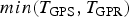
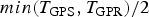
 $$e_T \le \min (T_{{\rm GPS}}, T_{{\rm GPR}} ).$$
In all cases discussed, a, b, bI and bII the errors e T have the same sign, thus indicating the existence of a bias in the trace positioning. If this bias is not corrected, we should use the maximum value of e T to conservatively characterize ε T ,
 $$\varepsilon _{T} = \min (T_{{\rm GPS}}, T_{{\rm GPR}} ).$$
However, if the error in position is not negligible we suggest correcting such a bias. In cases a, bI and bII, e
T
is a random variable with a uniform distribution between 0 and
 $min(T_{{\rm GPS}}, T_{{\rm GPR}} )$
, with a mean value of
$min(T_{{\rm GPS}}, T_{{\rm GPR}} )$
, with a mean value of
 $min(T_{{\rm GPS}}, T_{{\rm GPR}} )/2$
(the bias,
$min(T_{{\rm GPS}}, T_{{\rm GPR}} )/2$
(the bias,
 $\mu (e_{T} )$
) and a standard deviation
$\mu (e_{T} )$
) and a standard deviation
 $(\sigma (e_{T} ))$
of
$(\sigma (e_{T} ))$
of
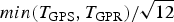 $min(T_{{\rm GPS}}, T_{{\rm GPR}} )/\sqrt {12} $
. Consequently, if coordinates are reassigned to traces, correcting the bias results in a significant reduction of ε
T
. Depending on the GPR profiling speed, this bias correction could be significant or negligible.
$min(T_{{\rm GPS}}, T_{{\rm GPR}} )/\sqrt {12} $
. Consequently, if coordinates are reassigned to traces, correcting the bias results in a significant reduction of ε
T
. Depending on the GPR profiling speed, this bias correction could be significant or negligible.
Case aI is the result of applying, in case a, the bias correction to e T (Fig. 10), while cases bIII and bIV are the results of applying the corresponding bias corrections to bI and to bII respectively.
The parameters defining the uniform random variable e T for all the cases discussed above are shown in Table 3. The right column of the table shows the corresponding ε T value.
Parameters associated with the uniform random variable e T, in the cases discussed in the text
All errors discussed in this appendix represent uncertainties in the times of acquisition of GPS positioning by the GPR traces. Thus, according to Eqn (9) they must be multiplied by the profiling velocity to obtain the errors in positioning due to the movement in the profiling direction. Following the same rationale, the bias in e T must be corrected moving the coordinates of the traces forward in the direction of movement, a distance equal to the bias in e T times the profiling velocity. Both the profiling velocity and the direction of movement can be easily estimated from the coordinates and recorded time in subsequent traces.


 Open access