2.1 Denoising workflow

In this paper, a 3D DL denoising framework is proposed to reduce the time and cost associated with traditional manual denoising processes (see Figure 1). This workflow presents an adaptive denoising methodology for diverse tunnel point cloud quality, while the trained model is tailored to the specific inspection environment by the input parameters. The following section demonstrates this process with an example from the VCP 16 section in the DPT dataset. The flowchart of this framework consists of four phases: (1) point cloud visual assessment, (2) synthetic data generation, (3) training with the RandLA-Net DL architecture, and (4) application to the infrastructure point clouds.

Figure 1. Flowchart of proposed denoising methodology (algorithm in (Hu et al., Reference Hu, Yang, Xie, Rosa, Guo, Wang, Trigoni and Markham2022; Lin et al., Reference Lin, Sheil, Zhang, Zhou, Wang and Xie2024)).

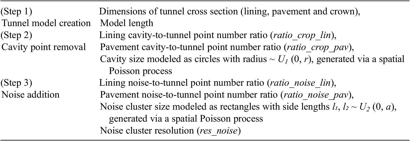
In the first phase, key parameters for synthetic data generation are quantified as per Table 1. The tunnel cross-section adopts either circular or elliptical profiles, vertically truncated at a 2.5 m vertical clearance to emulate road pavement obstruction. Cavity defects are defined by volume ratio with diameters 0-r cm, whereas noise clusters follow spatial Poisson distribution having rectangular shapes. In the second phase, the synthetic data are generated in three steps: building the uniform tunnel section, removing cavity points and adding noise clusters, as described in the following content:

1. 1) Tunnel model creation: the geometry of the tunnel cross-section can be defined according to the dimensions specified in the tunnel technical drawings, including elements such as lining, pavement, and crown. The tunnel length is determined to maintain a balance between the computational load for training and the amount of training information required.

2. 2) Cavity removal: The cavity in a tunnel point cloud model represents the absence of points that should have been captured in the tunnel model. It results from insufficient texture near smooth tunnel surfaces. The extent of cavities is quantified by proportionally removing points in a circular shape from the tunnel model initially created. Two groups of key parameters in Table 1 determine the condition of cavity defects: the ratio of cavity points to total tunnel points and the physical dimensions (diameter of the circle) of the non-textured areas on the tunnel surface.

3. 3) Noise addition: Similarly, noisy points are spurious artifacts that are not part of the true tunnel structure. Such noise is introduced by proportionally adding points in rectangular-shaped areas to mimic noise clusters. A random generation of the cavities and the noise is achieved by a spatial Poisson distribution with similar parameters in Table 1.

Table 1. Input parameters adopted for the synthetic data generation algorithm

For instance, in the DPT dataset, an appropriate model length is determined to be 40 m according to the tunnel dimension. This model length provides enough segmentation data for training and saves computational costs. After selecting the input parameters, the synthetic data generation algorithm produces labeled point clouds. This phase simulates realistic noise distributions caused by image stitching artifacts, thereby removing the need for manual annotation.

In the third phase, the DL model is trained using the RanDLA-Net algorithm, enabling segmentation of the point cloud based on spatial information.

2.2 Synthetic dataset preparation

Figure 2 illustrates an example synthetic dataset generated for DPT comprising three main classes of points: pavements (red), linings (green), and noise (blue). In this way, the proposed method produces fundamental characteristics of real-world point cloud data. In this study, the generation of the training and validation datasets is achieved using the synthetic data generation algorithm. There are 16 synthetic training datasets and 4 validation datasets. Advantages of synthetic point clouds include a substantial increase in efficiency and accuracy of annotation compared to a manual approach, particularly for noise which is commonly the minority class in a highly imbalanced dataset, whose annotation inevitably subjects to human errors. Additionally, the original real DPT dataset alone is insufficient for effective training, whereas the use of synthetic data ensures sufficient data volume.

Figure 2. Illustration of one realization of the synthetic dataset containing noise clusters and cavities (green: tunnel linings, blue: noise, red: road pavement), and zoomed image point clouds from VCP 16 test dataset.

2.3 3D DL method

In the fourth phase of the flowchart in Figure 1, the 3D DL algorithm is trained on the synthetic training dataset to generate a prediction model of the inspected area. The 3D DL RandLA-Net model (Hu et al., Reference Hu, Yang, Xie, Rosa, Guo, Wang, Trigoni and Markham2022; Lin et al., Reference Lin, Sheil, Zhang, Zhou, Wang and Xie2024) is adopted to train and validate with synthetic datasets, due to its advantage of processing large-scale point clouds while preserving complex geometric structures. Figure 3(a) illustrates the underlying principles of the RandLA-Net architecture. First, random down-sampling is used to reduce the computational cost whilst retaining key features. From left to right, the layers (1) to (3) in Figure 3(a) describe two local feature aggregation processes. Local spatial encoding (L) is used to extract valuable spatial information and attentive pooling (A) is used for information aggregation. As a result, one point in the colored circles is used to represent several neighbor points, and this process progressively increases the receptive field size with minimal information loss.

Figure 3. Principle of RandLA-Net (a) Schematic illustration and (b) Down-sampling performance (Hu et al., Reference Hu, Yang, Xie, Rosa, Guo, Wang, Trigoni and Markham2022).

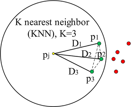
Figure 3(b) provides a down-sampled example from the synthetic dataset where the DL method reduces the number of points by three orders of magnitude whilst retaining important features. In contrast, traditional filters use a fixed number of points to find those close to the centers of point clusters, regardless of the real-world geometry of the point clusters. For instance, Figure 4 presents a Sigma SOR filter, which statistically analyses the K-nearest neighboring points ( $ {p}_i $ ) to each point $ {p}_j $ to calculate the threshold distance for point denoising (K = 3 in this particular example). The analysis is conducted to establish a threshold formula:

(1) $$ {D}_{max}=i+{n}_{\sigma}\cdotp \sigma $$

where $ i $ is the global average distances from each point to its K nearest neighbor points, and $ {n}_{\sigma } $ is a user-defined multiplier of the deviations ( $ \sigma $ ). For $ {p}_i $ , if the distance between $ {p}_i $ and $ {p}_j $ ( $ {D}_i $ ) exceeds threshold $ {D}_{max} $ , it will be considered noise (red points in Figure 4). This method presupposes that noise points are distributed in a uniform manner around the surface, which is not the case around corners in tunnels. Consequently, the Sigma SOR filter struggles to preserve geometric features in intricate underground structures, even though it may be well-suited for denoising smooth surfaces.

Figure 4. Schematic illustration of the principle of traditional filters.

The RandLA-Net is trained using a batch size of 4 and a learning rate of 0.01. The network has 5 layers with subsampling ratios of (Attard et al., Reference Attard, Debono, Valentino and Di Castro2018; Xu and Yang, Reference Xu and Yang2020), and the output dimensions of the layers are [16, 64, 128, 256, 512]. The above hyperparameters apply to all case studies. Once trained, the model is applied to identify noise in the unseen raw real-world infrastructure point cloud.

2.4 Evaluation metrics

Model training was performed on a consumer-grade computer with NVIDIA GeForce RTX 3080 Ti GPU and Intel core i9 12900K CPU. Training of a 40 m model over 100 epochs takes around 16 hours. The cross-entropy loss (Schult et al., Reference Schult, Engelmann, Hermans, Litany, Tang and Leibe2023; Kolodiazhnyi et al., Reference Kolodiazhnyi, Vorontsova, Konushin and Rukhovich2024) is used for the semantic segmentation of the point clouds, and the overall accuracy (OA) and mean intersection over union (mIoU) are used as evaluation metrics for these imbalanced datasets. These metrics are calculated to evaluate the training performance in each iteration (Rainio et al., Reference Rainio, Teuho and Klén2024):

(1) $$ {\displaystyle \begin{array}{c} OA=\frac{\sum_{i=1}^n{TP}_i\;}{n}\end{array}} $$

(2) $$ {\displaystyle \begin{array}{c} IoU=\frac{\mathrm{TP}}{\mathrm{TP}+\mathrm{FP}+\mathrm{FN}}\end{array}} $$

(3) $$ {\displaystyle \begin{array}{c} mIoU=\frac{1}{n}\sum \limits_{i=1}^n Io{U}_i\end{array}} $$

Where OA is overall accuracy, n is the total number of classes, IoU (and $ Io{U}_i $ ) is Intersection over Union (and for the ith class), TP (and $ {TP}_i $ ) is the number of true positives (and for the i-th class), FP is the number of false positives, FN is the number of false negatives, and mIoU represents the mean intersection over union.

3.1 Data acquisition

DPT is one of the longest urban road tunnels in Europe. The DPT twin tunnel structure exhibits tunnel lining deformation and surface defects that have developed over time, necessitating regular structural health condition assessments. The inspection area covers the Southbound Bore (SB) and the Northbound Bore (NB), connected by vehicle cross passages (VCPs), as shown in Figure 1. Inspections focused on the layby tunnel within the “VCP 16” area measuring 40 m in length along the traffic direction, which displayed the most significant surface defects compared to the other sections of the tunnel. In the zone of interest (the inspection area), there are additional adjoining structures, such as lay-by tunnels and VCPs at intervals of 1 km, components, such as fire hoses every 65 m, and telephone niches every 250 m. The DPT lining encompassing the abovementioned structures and components, was inspected, resulting in a 3D digital model of the inspected section (see Figure 5).

Figure 5. 3D visualization of DPT VCP 16 section derived from UAV images (left SB connected to right NB via VCP).

The visual data acquisition platform used is a C2 class DJI Mavic 2 Enterprise Dual. Images were captured using a pre-programmed reactive UAV specifically adapted for automatic and stable inspections in road tunnels such as DPT (Zhang et al., Reference Zhang, Hao, Zhang and Li2024). Figure 6 illustrates the UAV inspection environment under dim lighting conditions. The tunnel linings and road pavement are visible, but the tunnel crown lacks sufficient visual details and is excluded from the UAV inspection. The images were taken from a distance of approximately 3 m from the tunnel lining surface with a resolution of 4056 × 3040 pixels. A total of 2494 images were used for tunnel model reconstruction, totaling 13.3 GB. The inspection required multiple flights for safety reasons, and to account for possible changes in the inspection environment, with 30% of the images were recaptured, potentially introducing artifacts and necessitating data cleaning. The presence of noise in image point clouds introduces noticeable surface roughness, adversely affecting the extraction of spatial information from the tunnel linings. In the context of tunnel health condition assessment, it is imperative to utilize accurate data, free from noise, to ensure reliable outcomes.

Figure 6. UAV inspection area as part of VCP 16 section in DPT.

3.2 Point cloud generation

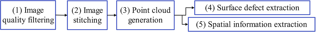
The image point cloud is generated to capitalize on the paired color and positional information, thereby facilitating the concurrent identification of defects and deformation. Figure 7 outlines the primary image processing workflow containing steps (1) to (5) illustrated by Figure 8(1) to (5) for generating a UAV image point cloud from individual images. The image quality filtering step (1) removes blurry images that could cause misalignment of hyperspectral features like edges or corners (Figure 8(1)). The image stitching step (2) aligns images in 3D space using feature matching to create digital models of tunnel linings using the software Pix4Dmapper (Zhang et al., Reference Zhang, Hao, Zhang and Li2024), with Figure 8(2) showing the software interface during this process. The numeric label in the top-left corner (e.g., “DJI_0407”) corresponds to the original image sequence number containing a specific example feature occurrence. The subsequent step (3) in Figure 8(3), point cloud generation, produces point clusters containing color or brightness information. The step (4), defect and spatial information extraction, yields paired datasets crucial for structural health analysis. Surface defects are identified and highlighted with distinct colors in Figure 8(4) (cracks in red, and water leakage in yellow box). In this workflow, image-based analysis is used to detect defects such as cracks and water leakages. The point cloud then provides positional information to accurately locate and size these defects. The DL-segmented point clouds, however, are not used for direct defect detection, but rather to ensure geometric fidelity of the tunnel lining for deformation analysis. Tunnel lining is divided into various zones according to the density of defects. The structural spatial information is incorporated into the DSM in Figure 8(5), which is displayed as depth images and can be extracted using GIS software.

Figure 7. Overview of point cloud processing workflow.

Figure 8. Illustration of point cloud processing steps: (a) Image quality filtering, (b) Image stitching from multiple views (Orange cross: tie points; Green cross: control points), (c) Point cloud generation, (d) Defects from orthomosaic, and (e) Depth image from DSM.

The tunnel model reconstruction process is highly feature-sensitive, particularly to elements such as tunnel fissures, structural components, and edges, leading to non-uniform point cloud density. Under low-light conditions, UAV drifting can result in the generation of cavities, artifacts, and rough surfaces. These issues often stem from conflicts or the lack of hyperspectral information. Potential approaches to enhance the quality of tunnel model reconstruction include addressing geofencing-related point absences, improving sensor quality, and increasing the number of inspection views. While higher-quality sensors and additional inspection views could alleviate some of these limitations, the constrained tunnel environment and safety-related restrictions often prevent optimal acquisition strategies. As such, developing denoising techniques that can operate effectively on imperfect datasets is essential for practical tunnel monitoring workflows.

3.3 Image point cloud deficiencies

Image point cloud deficiencies, including cavities, noise, and spurious rough surfaces, can be identified from the spatial distribution of the points. Figure 9 gives the extracted cross-sections of the tunnel lining from the manually denoised output, with data sourced from both the bored sections and the layby sections. Figure 9(a) shows the overall extraction map in the plan view, where two groups are marked with A–F and (1)–(4), respectively:

1. 1) Labels A to F represents the extraction positions used to investigate tunnel behavior near the VCP structure, consistent with relevant prior research (Zhang et al., Reference Zhang, Wang and Li2024). These extraction points are approximately evenly spaced to ensure data consistency while avoiding obstacles;

2. 2) Labels (1)–(4) represent examination sections, which are control sample locations used to evaluate the effectiveness of noise removal through circle fitting analysis. Specifically, Figure 9(b) shows the tunnel profile at examination Sections (1) to (3), with noise clusters highlighted.

Figure 9. Example of poor-quality cross-sectional extractions: (a) overall extraction map in plan view (two groups marked A to F and (1)–(4)); (b) tunnel lining profiles at examination sections (1)–(3) showing noise clusters; (c) details of tunnel circle fitting (on bored sections (B1 and B2) and layby sections (L)).

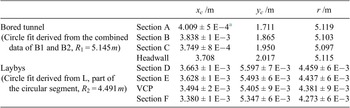
A high-quality point cloud enables quantification of surface defects and the assessment of tunnel geometry. However, when comparing the tunnel’s design specification with the acquired inspection data at key locations (see Figure 9(a)), the original DSM derived from the image point cloud inevitably contains greater errors than the tunnel deformation measurements. Therefore, these measurements must be denoised. Figure 9(c) illustrates the tunnel linings, with the bored sections labeled B1 and B2 and the layby sections denoted L. Also shown are the dimensions of the fitted tunnel diameter in the bored sections (modeled as circles) and layby areas (modeled as multi-center circles). Cross-sectional extractions (see Figure 9(b)) were used to represent the inspected part of the tunnel’s configuration. Based on the as-built design (see Figure 9(c)), these sections should exhibit smooth circular or multi-center circular surfaces under undeteriorated tunnel condition.

The scale of noise is evaluated from the characteristics of the circles fitted to the DSM extractions. While the noise assessment is influenced by tunnel deformation, the noise clusters, which typically present as surface roughness, occur on a scale larger than the actual deformation of the tunnel lining. Hence, the noise level is assessed using the confidence interval of circle radii and centers, as listed in Table 1. A closer fit to the designed geometry of the bored and layby sections ( $ {R}_1 $ and $ {R}_2 $ respectively) indicates fewer instances of clustered noise and better reconstruction accuracy, while a smaller confidence interval indicates less influences from the noise clusters.

In this study, manual point denoising was performed for comparison with later automated methods. It is worth noting that such manual processes remain subjective, prohibitively labor-intensive and introduce file encoding issues. Outlier removal is focused on areas near the edges of the tunnel linings and in areas with color variation. Comparisons of noise-free cross-sections in Table 1 reveals important structural health insights. For example, a slightly decreasing radius from sections D to F is observed, which suggests greater local compression near layby sections. This may be attributed to the diminished soil arching effect, as the soil is replaced by the cross-passage tunnel (Li et al., Reference Li, Soga and Wright2015). Between the twin tunnels, higher stiffness is observed on the east sides of both bores, especially over the right bracelet-shaped tunnel bend, due to increased compression resistance. Additionally, localized strengthening is observed around the headwall structures. Findings from previous research (Chao, Reference Chao2023) for the same inspection area verify this deformation mechanism data. This information is critical for structural analysis and integrity assessment, making denoising an essential step to improve accuracy (Table 2).

Table 2. Circle fit details of SB cross sections A–F (center coordinates (x_c, y_c) and radius r) together with mm-level fitting error

^a Standard errors <5E-4 are omitted for brevity; larger errors are listed for circle fitting uncertainty.

4.1 Experimental setting and model performance

The proposed denoising method is tested on two real-world cases: DPT and Wuxi metro. Application to DPT is first considered here. Each synthetic training and validation dataset contains 102,400 points. The parameters of the noise-free data in the synthetic model were chosen to mirror those of the original point cloud dataset, ensuring the denoised data was representative. A uniform cross-section from the layby area, representing the majority of the tunnel’s length (see Figures 5 and 8), was used in the synthetic dataset to build the tunnel geometry. The cross section’s multi-center circle shape was simplified to an ellipse with major and minor axes of 7.42 m and 5.18 m, respectively. The ellipse was truncated at heights of ±2.8 m to represent the ceiling and pavement. The tunnel model has a total length of 40 m. Its inner width varies at the headwall and VCP. The trained model was tested on both the bored and layby sections, and the results were combined to produce a denoised point cloud covering the entire tunnel length. The original image point cloud is down-sampled to maintain a resolution of 10 mm to preserve details and for training efficiency; the synthetic model shares the downsampling voxel size of 0.01 m.

The noise and cavity distribution in the DPT model are configured based on preliminary assessments from the image point cloud data. The noise is added with ratio_noise_lin set to 5% and ratio_noise_pav set to 1%. It is introduced at a spatial resolution of 0.05 m, and the dimensions of noise rectangular shapes are randomly ranging from 0 × 0 m to 0.5 × 0.5 m. Additionally, cavities are introduced to emulate imperfections in the image data acquisition, with ratio_crop_lin set to 50% and ratio_crop_pav to 10%. The radii of the circular cavities are randomly distributed between 0 m and 1 m.

Figure 10 illustrates the training process on the synthetic datasets. It shows that the DL model converges quickly and achieves good performance on both the training and validation data over 100 epochs, achieving a high mIoU score. Importantly, both training and validation loss decrease sharply and plateau to small and comparable labels indicating effective training without overfitting and thus is able to generalize between the datasets. After approximately 20 epochs, these evaluation metrics remain steady, indicating that it has reached an optimal state of learning. The consequent dataset prediction takes several minutes per model, showcasing advantage of efficiency for long-term or large dataset prediction over manual labeling.

Figure 10. Training process of RandLA-Net on the DPT synthetic dataset over 100 epochs.

Figure 11 shows the original raw point cloud (Figure 11(a)), the DL prediction of the primary segmented data in the DPT southbound bore (Figure 11(b)), and the DL-segmented data with noise removed (Figure 11(c)). The DL segmentation results reveal the present of noise around the tunnel lining. The road pavement and tunnel linings are generally well-segmented, but the narrow pedestrian area on the road pavement is not recognized, as it was not modeled in the synthetic data simulator. After removing the noise class, Figure 11(c) reduces noise points near low fidelity areas in the original model, including the southern part with many cavities, structural complex areas like fire door areas, and VCP areas.

Figure 11. Data visualization of the point cloud applied to SB in VCP 16: (a) Original raw real point cloud data, (b) DL-segmented data into primary classes, (c) DL-segmented following removal of noise.

4.2 Qualitative observations

DPT visualization model contains bulk noise and artifacts (similar to comet tail artifacts in medical imaging). Bulk Noise is observed as randomly distributed noise cover the majority of the model surface. It causes a lower resolution and grainy texture from the noises of the sensors. The artifacts, on the contrary, occurs more frequently on structural edges as fading lines due to various reasons, taking the incapacity in processing as an example.

Figure 12 illustrates the segmentation of the NB point cloud. Figure 12(a) presents the entire structure, focusing on two areas: the road pavement, highlighted by the green box and the tunnel lining edge, highlighted by the red box. A closer examination of them is shown in Figure 12(b) and (c), respectively. The data is presented in two classes: the predicted noise-free structure (black points) and the predicted noise (blue points). And that the resulting noise-free points in pavement section span an absolute range of 0.2 m and the noise spans an absolute range of 2 m. In contrast, for tunnel lining, the noise-free point and the noise span an absolute range of 0.2 m and 0.5-meter range, respectively. Overall, this technique effectively reduces artifact noise in targeted areas, enhancing the clarity and precision of the structural model.

Figure 12. Deep learning-based point cloud denoising shown in (a) the whole southbound, (b) a 14 m long road pavement, and (c) crown-lining border.

Figure 13 illustrates the segmented photogrammetric point cloud of the SB layby tunnel generated from multi-temporal UAV image acquisitions across three inspection dates (September 2022 to March 2023). Dense noise clusters observed behind the fire door (highlighted in blue) predominantly originate from two synergistic factors: (1) temporal redundancy caused by repeated UAV flights capturing transient objects, including parked maintenance vehicles, temporary equipment installations, and dynamic door positions (open/closed states during interventions), which were misinterpreted as persistent structural features during Structure-from-Motion (SfM) processing and (2) environmental variability induced by LED lighting upgrades midway through the monitoring period, resulting in illumination fluctuations between scans. These photometric inconsistencies degraded feature matching accuracy during image registration, propagating positional errors as false 3D points.

Figure 13. Segmentation results of the (a) SPT SB layby tunnel, with two zoomed-in examples of noise: (b) near cavities, and (c) behind the fire door.

Figure 13 provides a three-dimensional visualization of the point cloud, where the different classes are again identified by the different colors. Noise points are particularly noticeable near the edges of the tunnel lining and on top of the pavement. These areas correspond to artifacts near structural edges or erroneous data captured behind the fire door during scanning. The proposed effectively eliminated 7232 spurious points (84% of the initial 8560 noise points) in the fire door’s closed-state region, improving the reconstructed model’s geometric accuracy (RMSE reduction: from 2.6 m to 0.2 m). Moreover, it can be seen that the present DL method effectively retains two structural and geometric details, such as the junction between tunnel walls and the road surface.

In contrast, Figure 14 shows the point cloud using a traditional SOR approach for three different combinations of K and σ, representing the number of points used for mean distance estimation and the factor of deviation for outlier detection, respectively. The SOR method’s reliance on neighborhood-based statistical thresholds (Eq.1) introduces edge-blurring artifacts, particularly in geometrically complex regions. As shown in Figure 14, under K = 10, σ = 1 and K = 5, σ = 1, tunnel lining textures are eroded despite achieving better noise removal effect behind fire door. This demonstrates a critical trade-off: larger K improves global denoising but sacrifices local geometric fidelity. This is because traditional methods treat all points in the data equally, without considering whether a point is part of a flat surface, edge, or corner. These traditional denoising methods often lose detail in sharp features like corners, while the proposed method preserves geometric details, making it ideal for precision-critical applications.

Figure 14. Sensitivity analysis of SOR parameters defined in Eq. 1: (a) K = 10, σ = 1: over-smoothing regime with critical detail loss on tunnel lining (b) K = 5, σ = 1, over-smoothing regime (c) K = 5, σ = 2: under-filtering regime with residual noise clusters near fire door joints.

4.3 Quantitative tunnel geometry examinations

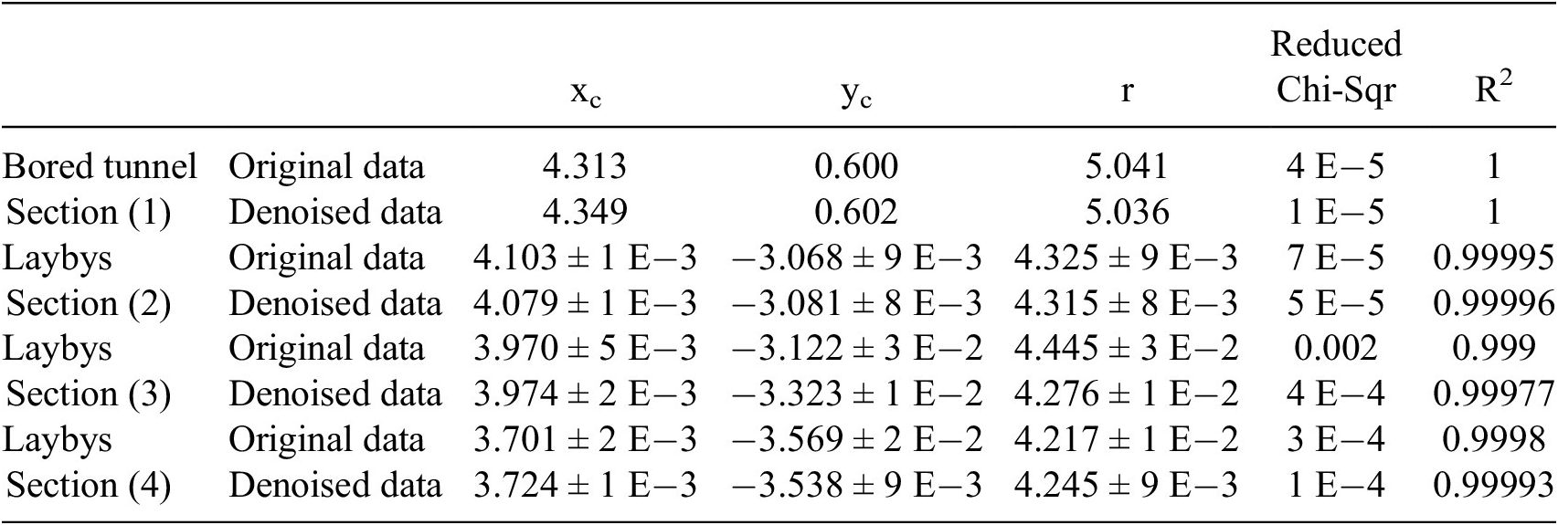
Figure 15 compares tunnel cross-sectional geometries before and after denoising at four inspection locations: (1) shown in Figure 15(a) and (2)–(4) in Figure 15(b). Table 3 quantifies the circle-fitting performance, deviations in center coordinates (maximum shift: 201 mm) and radii (mean difference: 169 mm) between denoised and raw point clouds. It reflects inherent uncertainties in tunnel scanning conditions. These magnitudes are attributable to dynamic acquisition artifacts and denoising algorithmic tolerance. Notably, these sub-200 mm discrepancies represent operational-level precision for infrastructure inspection, where critical alert thresholds are typically set at >500 mm (ASCE 95-2023). The preserved correlation between denoised/raw datasets (Pearson’s r = 1) confirms methodological consistency despite absolute value differences.

Figure 15. Comparison of two fitted circles’ shapes before and after DL denoising in Northbound Bore (NB) (a) Examination section (1) (b) Examination sections (2), (3), (4) from right to left.

Table 3. Circle fit details of two example cross sections before and after DL denoising in NB (/m)

Denoising significantly improves fitting accuracy in high-noise regions (Sections 3) and 4). Particularly, it reducing local horizontal errors from 0.4 m to 0.2 m at most, while the radius narrows at most 17 cm on section (3) circled area in Figure14(b). Statistically, DL denoising reduces the reduced Chi-Square values by 74% in bored sections and at least 28% in layby sections with noise, with both models achieving coefficient of determination (R²) values exceeding 0.99. These millimeter-scale changes in the 3.5 m × 0.5 m local inspection zone, demonstrate critical sensitivity improvements for deformation assessment. Future extensions could incorporate elliptical fittings to analyze localized deformation patterns, particularly in regions showing asymmetric profile shifts.

5.1 Experimental setting

To evaluate the generalizability of the proposed workflow, an additional experiment was conducted utilizing TLS data from the Wuxi dataset (Lin et al., Reference Lin, Sheil, Zhang, Zhou, Wang and Xie2024). The tunnel comprises prefabricated concrete lining rings with a 2.75 m radius, horizontally truncated at the invert to interface with the road surface. Each segmented ring extends 1.5 m axially and incorporates engineered joints. The dataset also includes adjacent structures, including bolts, pipelines, and road surfaces. This high-fidelity data enables robust segmentation of individual lining segments, particularly for detecting service-stage deformations such as joint misalignments >2 mm or radial deviations exceeding 1.5% of the nominal radius.

The synthetic training dataset was generated with systematic noise simulation configured to approximate real-world TLS measurement artifacts. Lining noises was incorporated at a ratio of 5% (ratio_noise_lin = 0.05) along structural edges, while road surface noise was introduced at 1% density (ratio_noise_pav = 0.01). These noise elements were spatially distributed at a resolution of 0.05 m, with rectangular noise clusters randomly sampled within dimensional bounds of 0 × 0 m to 0.5 × 0.5 m to simulate irregular scanning noises. Cavity artifacts were explicitly excluded from the model on the smooth tunnel surfaces. For the RandLA-Net implementation, a 5-layer architecture was employed with progressive downsampling ratios of (Attard et al., Reference Attard, Debono, Valentino and Di Castro2018; Xu and Yang, Reference Xu and Yang2020), corresponding to feature dimension expansions from 16 to 512 channels. Training utilized a batch size of 4 and an initial learning rate of 0.01, optimized through gradient descent with momentum stabilization to mitigate high-noise sensitivity.

Figure 16 illustrates a synthetic point cloud where the structural component of interest (the lining) is identified in red and all other points (noise plus pavement) are again identified in blue. A limitation of this synthetic dataset is the difficulty in incorporating details such as tracks, bolts and pipelines. Each training dataset comprises 204,800 points, following downsampling with a voxel size of 0.04 m. The model validation results on the synthetic data achieve an OA of 98.88% and an mIoU of 97.18%, highlighting the method’s exceptional accuracy and efficacy in segmenting the synthetic data.

Figure 16. An exemplar synthetic point cloud in the Wuxi dataset.

5.2 DL model assessment

Figure 17 compares the DL denoising results (Figure 17(1)) to the manually segmented ground truth (Figure 17(2)). It can be seen the method demonstrates a high level of accuracy in removing non-lining structures, particularly bolts, pipelines, and tracks, which are not prioritized in the training dataset as primary structural details. However, certain discrepancies between the DL predictions and the ground truth are evident, particularly in the form of missegmented fragments within the road pavement. Furthermore, continuous pipelines near the surface at the tunnel crown and 2 m height were misclassified as tunnel linings. When applied to the real-world test set, the method achieves satisfactory results with an OA of 89.68% and an mIoU of 80.06%. While there is a slight decrease in performance when transitioning from synthetic to real-world data, these results still indicate robustness and an ability to generalize to different datasets well. Reasons for these differences in performance can be attributed to the expediency of the modeling process, which did not provide other data artifacts such as miscellaneous obstructions.

Figure 17. Segmentation results and ground truth in the Wuxi Dataset (a) Segmented result using machine learning (b) Ground truth from manual annotation.

5.3 Model comparison

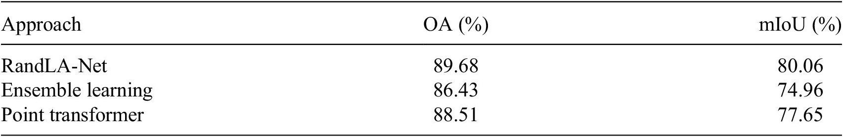
To validate the effectiveness of the RandLA-Net deep learning network adopted in this paper, representative approaches were used for comparisons, i.e., ensemble learning and Point Transformer.

Since there is no intensity or color information in the synthetic data, the input features of the base model consist of three-dimensional coordinates (X, Y, Z) and normal vectors (Nx, Ny, Nz). The normal vectors were calculated using 10 nearest points. The K-nearest neighbors (KNN), gradient boosting (GB), support vector machine (SVM), extra trees (ET), random forest (RF), and bootstrap aggregating (bagging) algorithms were chosen as the base models. The basemodels were trained independently using the training set. The hyperparameters in the basemodels were optimized by grid search. Then the outputs of basemodels were input into the metamodel for another round of training. The metamodel adopts the stacking strategy and uses logistic regression. The model training workflow was the same as that in the previous work (Peng et al., Reference Peng, Lin, Xia, Yu and Wang2024). As a result, the OA and mIoU of the meta model are 84.43% and 74.96%, respectively. The results highlight the adaptability of the adopted deep learning algorithms for the specific task. The potential reason is that the synthetic data includes only basic geometric information, hindering the ensemble learning method from effectively learning the advanced features in the real-world point clouds.

Additional comparison was implemented by replacing the local feature aggregation module in RandLANet with Point Transformer (Zhao et al., Reference Zhao, Jiang, Jia, Torr and Koltun2021). All other experiment setups and hyperparameters were kept unchanged to ensure rigorous comparison. The OA and mIoU of the trained model using Point Transformer are 88.51% and 77.65%, respectively, showing compromised performance compared to RandLA-Net. The results indicate that the feature aggregation module in RandLA-Net, designed with a self-attention mechanism, is more suitable for tunnel point cloud segmentation.

The segmentation performance of the compared approaches is listed in Table 4. It is proven that the synthetic data are effective for different approaches, with mIoU more than 74%, although there are slight differences in segmentation performance. Further, the segmentation results of the compared approaches are presented in Figure 18. Despite the numerical differences in the evaluation metrics, all three compared approaches yield satisfactory performance in recognizing structural points in the tunnel point clouds, demonstrating the feasibility of synthetic data.

Table 4. Segmentation performance of compared approaches

Figure 18. Segmentation results of compared approaches.