






1 Introduction
A folklore conjecture in number theory states that any
$k\in \mathbb {Z}$
 , not congruent to
$\pm 4$
, not congruent to
$\pm 4$
 modulo
$9$
modulo
$9$
 , admits a representation as a sum of three cubes of integers. The state of the art around this difficult problem is summarised in recent work by Wang [Reference Wang57], where a modern form of the circle method is developed to prove the conjecture for a positive proportion of integers k. Wang’s work is highly conditional, depending on an automorphy conjecture and GRH for certain Hasse–Weil L-functions, as well as the Ratios Conjecture from random matrix theory and a Square-Free Sieve Conjecture [Reference Wang57, Conjecture 1.6].
In this paper we investigate the analogous problem over the function field
$K=\mathbb {F}_q(t)$
 , with the aim of removing as many of the hypotheses as possible from [Reference Wang57]. Let
$\mathcal {O}=\mathbb {F}_q[t]$
, with the aim of removing as many of the hypotheses as possible from [Reference Wang57]. Let
$\mathcal {O}=\mathbb {F}_q[t]$
 denote the ring of integers of K and let
$k\in \mathcal {O}$
denote the ring of integers of K and let
$k\in \mathcal {O}$
 . In stark contrast to the case of
$\mathbb {Z}$
. In stark contrast to the case of
$\mathbb {Z}$
 , when
$\operatorname {\mathrm {char}}(\mathbb {F}_q)\ne 3$
, when
$\operatorname {\mathrm {char}}(\mathbb {F}_q)\ne 3$
 and
$q\notin \{2,4,7,13,16\}$
and
$q\notin \{2,4,7,13,16\}$
 , Serre and Vaserstein [Reference Vaserstein51, Lemma 1] have explicitly constructed linear functions
$a_ik+b_i$
, Serre and Vaserstein [Reference Vaserstein51, Lemma 1] have explicitly constructed linear functions
$a_ik+b_i$
 , with
$a_i\in \mathbb {F}_q^\times $
, with
$a_i\in \mathbb {F}_q^\times $
 and
$b_i\in \mathbb {F}_q$
and
$b_i\in \mathbb {F}_q$
 , such that
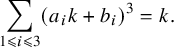
Vaserstein also gives more complicated polynomial constructions if
$q\in \{7,13\}$
 . In each case, the degrees of
$x,y,z\in \mathcal {O}$
. In each case, the degrees of
$x,y,z\in \mathcal {O}$
 solving
$x^3+y^3+z^3 = k$
solving
$x^3+y^3+z^3 = k$
 are
$\geqslant \deg {k}$
are
$\geqslant \deg {k}$
 , whereas one might hope for solutions of degree
$\sim \tfrac 13 \deg {k}$
, whereas one might hope for solutions of degree
$\sim \tfrac 13 \deg {k}$
 . Also, [Reference Vaserstein51] only constructs a bounded finite number of solutions for each k, and thus it remains open to produce an infinitude of solutions, or even a number of solutions tending to infinity with
$\deg {k}$
. Also, [Reference Vaserstein51] only constructs a bounded finite number of solutions for each k, and thus it remains open to produce an infinitude of solutions, or even a number of solutions tending to infinity with
$\deg {k}$
 .
.
According to [Reference Gallardo and Vaserstein24], when
$q=16$
 there is no known polynomial construction, but a direct adaptation of [Reference Colliot-Thélène and Wittenberg15, Lemme 4.5] shows that there are no local obstructions to the representation of k as a sum of three cubes from
$\mathcal {O}$
there is no known polynomial construction, but a direct adaptation of [Reference Colliot-Thélène and Wittenberg15, Lemme 4.5] shows that there are no local obstructions to the representation of k as a sum of three cubes from
$\mathcal {O}$
 and so it is natural to conjecture that most, or perhaps all,
$k\in \mathcal {O}$
and so it is natural to conjecture that most, or perhaps all,
$k\in \mathcal {O}$
 admit such a representation. When
$q\in \{2,4\}$
admit such a representation. When
$q\in \{2,4\}$
 , there are local obstructions at places of residue cardinality
$4$
, there are local obstructions at places of residue cardinality
$4$
 , because all cubes in
$\mathbb {F}_4$
, because all cubes in
$\mathbb {F}_4$
 lie in the proper subfield
$\mathbb {F}_2$
lie in the proper subfield
$\mathbb {F}_2$
 ; but most, or perhaps all,
$k\in \mathcal {O}$
; but most, or perhaps all,
$k\in \mathcal {O}$
 may still satisfy the Hasse principle, with a positive proportion then being representable. If
$\operatorname {\mathrm {char}}(\mathbb {F}_q)=3$
may still satisfy the Hasse principle, with a positive proportion then being representable. If
$\operatorname {\mathrm {char}}(\mathbb {F}_q)=3$
 , then
$\{x^3+y^3+z^3: x,y,z\in \mathcal {O}\}$
, then
$\{x^3+y^3+z^3: x,y,z\in \mathcal {O}\}$
 has density
$0$
has density
$0$
 in
$\mathcal {O}$
in
$\mathcal {O}$
 , however, because
$x^3+y^3+z^3 = (x+y+z)^3$
, however, because
$x^3+y^3+z^3 = (x+y+z)^3$
 .
.
To each smooth hyperplane section
$c_1x_1+\dots +c_6x_6=0$
 of the hypersurface

in
$\mathbb {P}^5_K$
 , for
$\boldsymbol {c}=(c_1,\dots ,c_6)\in \mathcal {O}^6$
, for
$\boldsymbol {c}=(c_1,\dots ,c_6)\in \mathcal {O}^6$
 , we shall see in § 3 that we can associate a Hasse–Weil L-function
$L(s,\boldsymbol {c})$
, we shall see in § 3 that we can associate a Hasse–Weil L-function
$L(s,\boldsymbol {c})$
 over K. Thanks to Grothendieck and Deligne [Reference Deligne20,Reference Grothendieck27], we know that these L-functions are actually rational functions of
$q^{-s}$
over K. Thanks to Grothendieck and Deligne [Reference Deligne20,Reference Grothendieck27], we know that these L-functions are actually rational functions of
$q^{-s}$
 that satisfy the Grand Riemann Hypothesis (GRH); that is, their zeros lie on the line
$\Re (s) = \frac {1}{2}$
that satisfy the Grand Riemann Hypothesis (GRH); that is, their zeros lie on the line
$\Re (s) = \frac {1}{2}$
 . Our main result relies on mean-value statistics of the ratio
$1/L(s,\boldsymbol {c})$
. Our main result relies on mean-value statistics of the ratio
$1/L(s,\boldsymbol {c})$
 over boxes of vectors
$\boldsymbol {c}\in \mathcal {O}^6$
over boxes of vectors
$\boldsymbol {c}\in \mathcal {O}^6$
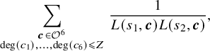
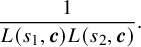
 ; we need an asymptotic formula for
as
$Z\to \infty $
 , where the distance from
$\Re (s_1),\Re (s_2)$
, where the distance from
$\Re (s_1),\Re (s_2)$
 to
$\frac {1}{2}$
to
$\frac {1}{2}$
 is sufficiently small compared to the quality of the error term. This is given by Conjecture 3.6 (R2), a special case of the Ratios Conjecture. The following is our main result.
Theorem 1.1. Suppose
$\operatorname {\mathrm {char}}(\mathbb {F}_q)> 3$
 and assume the Ratios Conjecture 3.6 for
$L(s,\boldsymbol {c})$
and assume the Ratios Conjecture 3.6 for
$L(s,\boldsymbol {c})$
 , as
$\boldsymbol {c}\in \mathcal {O}^6$
, as
$\boldsymbol {c}\in \mathcal {O}^6$
 varies. Then each of the following sets has positive lower density in
$\mathcal {O}$
varies. Then each of the following sets has positive lower density in
$\mathcal {O}$
 .
.
-
1. $\{x^3+y^3+z^3: x,y,z\in \mathcal {O}\text { monic}\}$
 .
. -
2. $\{k: x^3+y^3+z^3=k\text { is soluble in } \mathcal {O} \text { with max }\{\deg {x},\deg {y},\deg {z}\} \leqslant \lceil \frac {\deg {k}}{3} \rceil \}$
.


We remark that
$\deg (x^3+y^3+z^3) = 3\ \text {max}\{\deg {x},\deg {y},\deg {z}\}$
 for all monic polynomials
$x,y,z\in \mathcal {O}$
for all monic polynomials
$x,y,z\in \mathcal {O}$
 , when
$\operatorname {\mathrm {char}}(\mathbb {F}_q)> 3$
, when
$\operatorname {\mathrm {char}}(\mathbb {F}_q)> 3$
 , whence the set in (1) is a subset of the set in (2). In parts (6) and (7) of Theorem 11.1, we will strengthen Theorem 1.1, showing that we can take
$x,y,z\in \mathcal {O}$
, whence the set in (1) is a subset of the set in (2). In parts (6) and (7) of Theorem 11.1, we will strengthen Theorem 1.1, showing that we can take
$x,y,z\in \mathcal {O}$
 to be monic polynomials lying in any fixed subset of
$\mathcal {O}$
to be monic polynomials lying in any fixed subset of
$\mathcal {O}$
 of positive lower density. Throughout this paper, we think of q as being fixed. Thus all implied constants, and unspecified positive densities, are allowed to depend on q.
The set in (2) is known in Waring’s problem as the set of strict sums of three cubes, in the sense of Carlitz [Reference Gallardo and Vaserstein23, p. 2964]. We have already seen that the conclusions of the theorem are false if
$\operatorname {\mathrm {char}}(\mathbb {F}_q)=3$
 , where the sets in (1) and (2) have density
$0$
, where the sets in (1) and (2) have density
$0$
 . If
$\operatorname {\mathrm {char}}(\mathbb {F}_q)=2$
. If
$\operatorname {\mathrm {char}}(\mathbb {F}_q)=2$
 , then most of the proof of Theorem 1.1 still goes through, but some of the ingredients would need to be modified. We shall comment further on this in § 11.
The Ratios Conjectures were originally stated for automorphic L-functions over
$\mathbb {Q}$
 by Conrey, Farmer, et al. [Reference Conrey, Farmer, Keating, Rubinstein and Snaith16,Reference Conrey, Farmer and Zirnbauer17]. Their natural extension to
$\mathbb {F}_q(t)$
by Conrey, Farmer, et al. [Reference Conrey, Farmer, Keating, Rubinstein and Snaith16,Reference Conrey, Farmer and Zirnbauer17]. Their natural extension to
$\mathbb {F}_q(t)$
 has been explained by Andrade and Keating [Reference Andrade and Keating2]. The precise form of the Ratios Conjecture we need will be presented in § 3. It is plausible that the homological stability framework of Bergström, Diaconu, Petersen and Westerland [Reference Bergström, Diaconu, Petersen and Westerland5], together with Miller, Patzt, Petersen and Randal-Williams [Reference Miller, Patzt, Petersen and Randal-Williams43], could eventually resolve the particular form of the Ratios Conjecture needed in the present paper, for sufficiently large values of q. We defer the details of this to § 11.2, where we shall define a q-restricted form of the Ratios Conjecture, together with a strengthening of Theorem 1.1, in the shape of Theorem 11.1. Still working under the Ratios Conjecture, one can show that the set

has lower density approaching
$1$
 as
$A\to \infty $
as
$A\to \infty $
 , by adapting the proof of [Reference Wang54, Theorem 1.6]. Moreover, one can show that this set has upper density
$< 1$
, by adapting the proof of [Reference Wang54, Theorem 1.6]. Moreover, one can show that this set has upper density
$< 1$
 for any fixed
$A\in \mathbb {R}$
for any fixed
$A\in \mathbb {R}$
 , by adapting local density arguments of Diaconu from [Reference Diaconu21, § 1]. Both tasks are deferred to the sequel [Reference Browning, Glas and Wang8], in order to keep the present paper as clean as possible.
The Ratios Conjecture has already found application in the theory of rational points on elliptic curves over K. Thus, following the work of Katz–Sarnak [Reference Katz and Sarnak36], and Conrey et al. [Reference Conrey, Farmer and Zirnbauer17,Reference Conrey and Snaith18], it has been shown that Goldfeld’s Conjecture follows from the Ratios Conjecture for a suitable family of elliptic curve L-functions over K. This conjecture states that there is a density
$\frac 12$
 of curves with prescribed analytic rank
$r\in \{0,1\}$
of curves with prescribed analytic rank
$r\in \{0,1\}$
 , and therefore implies the Birch and Swinnerton-Dyer Conjecture (BSD) for a density
$1$
, and therefore implies the Birch and Swinnerton-Dyer Conjecture (BSD) for a density
$1$
 of curves. Whereas L-function ratios are directly related to analytic ranks and BSD, their connection to integral points and sums of three cubes in Theorem 1.1 is much less direct.
Our proof of Theorem 1.1 uses the second moment method and requires a detailed analysis of the counting function

for given
$P\in \mathcal {O}$
 , where
$|\cdot |$
, where
$|\cdot |$
 denotes the usual absolute value on K. We shall be interested in the size of
$N(P)$
denotes the usual absolute value on K. We shall be interested in the size of
$N(P)$
 as
$|P|\to \infty $
as
$|P|\to \infty $
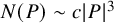
 . The Batyrev–Manin Conjecture suggests that an asymptotic formula of the shape
$N(P)\sim c|P|^3$
. The Batyrev–Manin Conjecture suggests that an asymptotic formula of the shape
$N(P)\sim c|P|^3$
 should hold, for a suitable constant
$c>0$
should hold, for a suitable constant
$c>0$
 . The best progress towards this is to be found in recent work of Glas and Hochfilzer [Reference Glas and Hochfilzer26], who use a function field version of the circle method to prove that

for any
$\varepsilon>0$
 , assuming only that
$\operatorname {\mathrm {char}}(\mathbb {F}_q)\neq 3$
, assuming only that
$\operatorname {\mathrm {char}}(\mathbb {F}_q)\neq 3$
 . It is worth emphasising that this bound is completely unconditional, unlike the parallel picture over
$\mathbb {Z}$
. It is worth emphasising that this bound is completely unconditional, unlike the parallel picture over
$\mathbb {Z}$
 , where the pioneering work of Hooley [Reference Hooley29,Reference Hooley33] and Heath-Brown [Reference Heath-Brown28] is conditional on GRH. Assuming that
$\operatorname {\mathrm {char}}(\mathbb {F}_q)>3$
, where the pioneering work of Hooley [Reference Hooley29,Reference Hooley33] and Heath-Brown [Reference Heath-Brown28] is conditional on GRH. Assuming that
$\operatorname {\mathrm {char}}(\mathbb {F}_q)>3$
 , our proof of Theorem 1.1 entirely rests on our ability to remove the
$\varepsilon $
, our proof of Theorem 1.1 entirely rests on our ability to remove the
$\varepsilon $
 from the upper bound (1.2). Ultimately we shall only manage to do so at the cost of assuming the Ratios Conjecture for the Hasse–Weil L-functions
$L(s,\boldsymbol {c})$
from the upper bound (1.2). Ultimately we shall only manage to do so at the cost of assuming the Ratios Conjecture for the Hasse–Weil L-functions
$L(s,\boldsymbol {c})$
 , as
$\boldsymbol {c}\in \mathcal {O}^6$
, as
$\boldsymbol {c}\in \mathcal {O}^6$
 varies. In fact,
$L(s,\boldsymbol {c})$
varies. In fact,
$L(s,\boldsymbol {c})$
 is only defined for generic vectors
$\boldsymbol {c}$
is only defined for generic vectors
$\boldsymbol {c}$
 , whereas we shall be able to handle the contribution from nongeneric vectors unconditionally, finding that they encode special subvarieties that contribute to
$N(P)$
, whereas we shall be able to handle the contribution from nongeneric vectors unconditionally, finding that they encode special subvarieties that contribute to
$N(P)$
 .
.
Our argument will broadly follow the path laid down by Wang [Reference Wang57] over
$\mathbb {Z}$
 , but with a variety of differences and refinements, some of which we have chosen to highlight here.
-
1. The L-functions $L(s,\boldsymbol c)$
carry less information over
$\mathbb {F}_q(t)$
than over
$\mathbb {Q}$
, since q-adic sums of local coefficients are collapsed into single global coefficients. Nonetheless, these are still the only L-functions that we need in our analysis, provided we choose our weight functions carefully, as suggested in the next item of this list. -
2. In order to avoid introducing character twists as in [Reference Browning and Vishe12], which would enlarge and complicate the form of the Ratios Conjecture needed, we restrict the class of weight functions that we use. This allows us to cleanly factor out the relevant oscillatory integral using symmetry ideas of Glas–Hochfilzer [Reference Glas and Hochfilzer26].
-
3. The precise automorphy hypotheses and Square-Free Sieve Conjecture required in [Reference Wang57] become unconditional over $\mathbb {F}_q(t)$
. For the former, we use Poincaré duality to carefully produce poles of exterior square L-functions. For the latter, we use an argument of Poonen [Reference Poonen45] on square-free values of multivariate polynomials. -
4. In Theorem 7.2 we prove a simple version of the Ekedahl sieve in positive characteristic for square-free moduli, which is sufficient for the applications in this paper. (A general prime moduli version for arbitrary global fields has been worked out by Bhargava–Shankar–Wang [Reference Bhargava, Shankar and Wang7].)
-
5. The bias in exponential sums that was discovered in [Reference Wang56, Lemma 7.7] was only worked out for diagonal cubic forms in six variables; in Proposition 10.6 we extend the argument to handle arbitrary nonsingular senary cubic forms. This requires new geometric insight on quadric bundles, via work of Beauville [Reference Beauville4].


Working over function fields, it is also natural to ask what happens in the limit as
$q\to \infty $
 . In this limit, methods of Coskun–Starr [Reference Coskun and Starr19] on rational curves in cubic hypersurfaces come into play. It follows from recent work of Kitagawa [Reference Kitagawa38] that
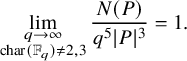
In addition, recent work of the second author [Reference Glas25] implies that
$N(P)\ll _{\deg P} q^5|P|^{3}$
 as long as
$\operatorname {\mathrm {char}}(\mathbb {F}_q)\neq 2,3$
as long as
$\operatorname {\mathrm {char}}(\mathbb {F}_q)\neq 2,3$
 , where the implied constant may depend on
$\deg P$
, where the implied constant may depend on
$\deg P$
 but not on q. Combining such estimates for
$N(P)$
but not on q. Combining such estimates for
$N(P)$
 with the second moment method, as in the proof of part (6) of Theorem 11.1, might then produce an unconditional analogue of Theorem 1.1 in the large q limit. We leave the details to the interested reader.
2 Background
In this section we collect some basic facts about the function field
$K=\mathbb {F}_q(t)$
 , which is equipped with the ring of integers
$\mathcal {O}=\mathbb {F}_q[t]$
, which is equipped with the ring of integers
$\mathcal {O}=\mathbb {F}_q[t]$
 . Let
$K_\infty =\mathbb {F}_q((t^{-1}))$
. Let
$K_\infty =\mathbb {F}_q((t^{-1}))$
 be the field of Laurent series in
$t^{-1}$
be the field of Laurent series in
$t^{-1}$
 . Let
$\mathcal {O}^+$
. Let
$\mathcal {O}^+$
 be the set of monic polynomials
$r\in \mathcal {O}$
be the set of monic polynomials
$r\in \mathcal {O}$
 ; this is analogous to the set of positive integers in
$\mathbb {Z}$
; this is analogous to the set of positive integers in
$\mathbb {Z}$
 . For
$M\in \mathbb {R}$
. For
$M\in \mathbb {R}$
 , we shall write
$\widehat {M}:= q^M$
, we shall write
$\widehat {M}:= q^M$
 . Any
$\alpha \in K_\infty \setminus \{0\}$
. Any
$\alpha \in K_\infty \setminus \{0\}$
 can be written uniquely as
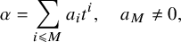
for some
$M\in \mathbb {Z}$
 and
$a_i\in \mathbb {F}_q$
and
$a_i\in \mathbb {F}_q$
 . Define
$|\alpha |:= \widehat {M}$
. Define
$|\alpha |:= \widehat {M}$
 ; then
$|\cdot |$
; then
$|\cdot |$
 naturally extends to
$K_\infty $
naturally extends to
$K_\infty $
 the absolute value on K induced by
$t^{-1}$
the absolute value on K induced by
$t^{-1}$
 . Moreover,
$K_\infty $
. Moreover,
$K_\infty $
 is the completion of K with respect to this absolute value. The analogue of the unit interval in
$K_\infty $
is the completion of K with respect to this absolute value. The analogue of the unit interval in
$K_\infty $
 is given by

Since
$K_\infty $
 is a local field, it can be endowed with a unique Haar measure
$\text {d} \alpha $
is a local field, it can be endowed with a unique Haar measure
$\text {d} \alpha $
 such that
$\int _{\mathbb {T}}\text {d}\alpha =1$
such that
$\int _{\mathbb {T}}\text {d}\alpha =1$
 . We shall extend the absolute value to
$K^n_\infty $
. We shall extend the absolute value to
$K^n_\infty $
 by
$|\boldsymbol {\alpha }|:= \text {max}_{1\leqslant i\leqslant n}|\alpha _i|$
by
$|\boldsymbol {\alpha }|:= \text {max}_{1\leqslant i\leqslant n}|\alpha _i|$
 and the Haar measure by
$\text {d} \boldsymbol {\alpha }:= \text {d} \alpha _1 \cdots \text {d}\alpha _n$
and the Haar measure by
$\text {d} \boldsymbol {\alpha }:= \text {d} \alpha _1 \cdots \text {d}\alpha _n$
 , for
$\boldsymbol {\alpha }=(\alpha _1,\dots , \alpha _n)\in K^n_\infty $
, for
$\boldsymbol {\alpha }=(\alpha _1,\dots , \alpha _n)\in K^n_\infty $
 . Finally, for each prime
$\varpi \in \mathcal {O}^+$
. Finally, for each prime
$\varpi \in \mathcal {O}^+$
 , we have an associated absolute value
$|\cdot |_\varpi $
, we have an associated absolute value
$|\cdot |_\varpi $
 on K, given by
$|a|_\varpi =q^{-v_\varpi (a)\deg \varpi }$
on K, given by
$|a|_\varpi =q^{-v_\varpi (a)\deg \varpi }$
 . We denote by
$K_\varpi $
. We denote by
$K_\varpi $
 the completion of K with respect to this absolute value and we write
$\mathcal {O}_\varpi := \{\alpha \in K_\varpi \colon |\alpha |_\varpi \leqslant 1\}.$
the completion of K with respect to this absolute value and we write
$\mathcal {O}_\varpi := \{\alpha \in K_\varpi \colon |\alpha |_\varpi \leqslant 1\}.$

Farey dissection
Dirichlet’s approximation theorem holds over K. That is, for any
$\alpha \in \mathbb {T}$
 and
$Q \in \mathbb {N} := \mathbb {Z}_{\geqslant 1}$
and
$Q \in \mathbb {N} := \mathbb {Z}_{\geqslant 1}$
 , there exist
$a\in \mathcal {O}$
, there exist
$a\in \mathcal {O}$
 and
$r\in \mathcal {O}^+$
and
$r\in \mathcal {O}^+$
 with
$\gcd (a,r)=1$
with
$\gcd (a,r)=1$
 and
$|a|<|r|\leqslant \widehat {Q}$
and
$|a|<|r|\leqslant \widehat {Q}$
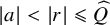 such that
$|r \alpha -a|<\widehat {Q}^{-1}$
such that
$|r \alpha -a|<\widehat {Q}^{-1}$
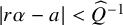 . By the ultrametric property, this is enough to obtain an analogue of a Farey dissection of the unit interval

for any
$Q\geqslant 1$
 . A full proof of this fact can be found in [Reference Browning and Vishe12, Lemma 4.2], for example.
Characters
For
$\alpha \in K_\infty $
 given by (2.1), we define

and set
$\psi (0)=1$
 , where as usual
$e(x) := \exp (2\pi i x)$
, where as usual
$e(x) := \exp (2\pi i x)$
 for
$x \in \mathbb {R}$
for
$x \in \mathbb {R}$
 . It is easy to see that
$\psi $
. It is easy to see that
$\psi $
 is a nontrivial additive character of
$K_\infty $
is a nontrivial additive character of
$K_\infty $
 , and that for
$x\in K_\infty $
, and that for
$x\in K_\infty $
 and
$N\in \mathbb {Z}_{\geqslant 0}$
and
$N\in \mathbb {Z}_{\geqslant 0}$
 , we have

Note that if
$x \in \mathcal {O}$
 , then (2.3) implies
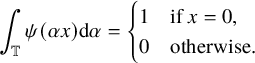
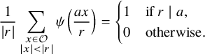
In addition, we will make frequent use of the following formula for exponential sums. If
$r,a \in \mathcal {O}$
 are such that
$r \neq 0$
are such that
$r \neq 0$
 , then
Poisson summation
We call a function
$w \colon K_\infty ^n \rightarrow \mathbb {C}$
 smooth if it is locally constant. Denote by
$S(K_\infty ^n)$
smooth if it is locally constant. Denote by
$S(K_\infty ^n)$
 the space of all smooth functions
$w \colon K_\infty ^n \rightarrow \mathbb {C}$
the space of all smooth functions
$w \colon K_\infty ^n \rightarrow \mathbb {C}$
 with compact support. For such functions the Poisson summation formula [Reference Browning and Vishe12, Lemma 2.1] holds in the following form.
Lemma 2.1. Let
$f \in K_\infty [x_1, \ldots , x_n]$
 and let
$w \in S(K_\infty ^n)$
and let
$w \in S(K_\infty ^n)$
 . Then we have

Delta method
Given a homogeneous cubic polynomial
$F\in \mathcal {O}[x_1,\dots ,x_n]$
 and a weight function
$w\in S(K^n_\infty )$
and a weight function
$w\in S(K^n_\infty )$
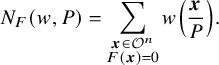
 , we are interested in the counting function
For a parameter
$Q\geqslant 1$
 to be specified later, we deduce from (2.2) and (2.3) that

where
$\sum ^{\prime }_{|a|<|r|} $
 means that we sum over
$a\in \mathcal {O}$
means that we sum over
$a\in \mathcal {O}$
 with
$\gcd (a,r)=1$
with
$\gcd (a,r)=1$
 only, and where

for
$\alpha \in \mathbb {T}$
 . As explained in [Reference Browning and Vishe12, § 4], we can use Poisson summation in Lemma 2.1 to evaluate
$S(\theta +a/r)$
. As explained in [Reference Browning and Vishe12, § 4], we can use Poisson summation in Lemma 2.1 to evaluate
$S(\theta +a/r)$
 , giving

where

and

Moreover, we will also consider averages of
$I_r(\theta ,\boldsymbol {c})$
 of the form

in which case we may write

Ultimately Q will be chosen so that
$|P|^{3/2}\asymp \widehat {Q}$
 .
.
The expression (2.5) is the starting point for our work and from now on we will mostly be concerned with estimating the integrals
$I_r(\theta ,\boldsymbol {c})$
 and the sums
$S_r(\boldsymbol {c})$
and the sums
$S_r(\boldsymbol {c})$
 . To keep notation simple, it is convenient to introduce the normalised sum

If
$r=r_1r_2$
 , where both
$r_1,r_2\in \mathcal {O}$
, where both
$r_1,r_2\in \mathcal {O}$
 are monic with
$\gcd (r_1,r_2)=1$
are monic with
$\gcd (r_1,r_2)=1$
 , the Chinese remainder theorem readily implies that

Therefore the prime factorisation of r will play an important role in our analysis. The letter
$\varpi $
 will generally denote a prime in
$\mathcal {O}^+$
will generally denote a prime in
$\mathcal {O}^+$
 .
.
Notation
Whenever the letter F appears from now on, we take

with
$n=6$
 . However, we will often work with a general choice of n to clarify the nature of arguments. Let

be the (primitive) dual form associated to F; it has degree
$3\cdot 2^{n-2}$
 . Let
$V\subset \mathbb {P}^{n-1}$
. Let
$V\subset \mathbb {P}^{n-1}$
 be the hypersurface defined by
$F=0$
be the hypersurface defined by
$F=0$
 . The dual form
$F^*$
. The dual form
$F^*$
 defines the dual variety
$V^*\subset \mathbb {P}^{n-1}$
defines the dual variety
$V^*\subset \mathbb {P}^{n-1}$
 of V, which parameterises hyperplanes that intersect V tangentially. Alternatively,
$V^*$
of V, which parameterises hyperplanes that intersect V tangentially. Alternatively,
$V^*$
 may be described as the closure of the image under the Gauss map
$V\to \mathbb {P}^{n-1}$
may be described as the closure of the image under the Gauss map
$V\to \mathbb {P}^{n-1}$
 given by
$\boldsymbol {x}\mapsto \nabla F(\boldsymbol {x})$
given by
$\boldsymbol {x}\mapsto \nabla F(\boldsymbol {x})$
 . From this description it is clear that

as an identity in
$K[x_1,\dots , x_n]$
 . Let
. Let

For each
$\boldsymbol {c}\in \mathcal {S}_1$
 , let
, let

Given
$r\in \mathcal {O}^+$
 and nonzero
$B\in \mathcal {O}$
and nonzero
$B\in \mathcal {O}$
 , we will sometimes write
$r\mid B^\infty $
, we will sometimes write
$r\mid B^\infty $
 to mean that
$\varpi \mid r\Rightarrow \varpi \mid B$
to mean that
$\varpi \mid r\Rightarrow \varpi \mid B$
 . This is equivalent to
$\text {rad}(r)\mid B$
. This is equivalent to
$\text {rad}(r)\mid B$
 , where
$\text {rad}(r)$
, where
$\text {rad}(r)$
 is the radical of r. In particular, we note that
$\mathcal {R}_{\boldsymbol {c}}^{\text {B}} = \{r\in \mathcal {O}^+: \text {rad}(r)\mid F^\ast (\boldsymbol {c})\}.$
is the radical of r. In particular, we note that
$\mathcal {R}_{\boldsymbol {c}}^{\text {B}} = \{r\in \mathcal {O}^+: \text {rad}(r)\mid F^\ast (\boldsymbol {c})\}.$

To connect
$S_r(\boldsymbol {c})$
 to Hasse–Weil L-functions, we define further quantities. Given a finite field k, let
$\mathcal {V}(k)$
to Hasse–Weil L-functions, we define further quantities. Given a finite field k, let
$\mathcal {V}(k)$
 be the set of k-points on the variety
$F(\boldsymbol {x})=0$
be the set of k-points on the variety
$F(\boldsymbol {x})=0$
 in
$\mathbb {P}^{5}_{k}$
in
$\mathbb {P}^{5}_{k}$
 , let
$\mathcal {V}_{\boldsymbol {c}}(k)$
, let
$\mathcal {V}_{\boldsymbol {c}}(k)$
 be the set of k-points on the variety
$F(\boldsymbol {x})=\boldsymbol {c}\cdot \boldsymbol {x}=0$
be the set of k-points on the variety
$F(\boldsymbol {x})=\boldsymbol {c}\cdot \boldsymbol {x}=0$
 in
$\mathbb {P}^{5}_{k}$
in
$\mathbb {P}^{5}_{k}$
 , and let

where
$\#{ \mathbb {P}^d(k) } = ((\# k)^{d+1}-1)/((\# k)-1)$
 . Next, let

For primes
$\varpi \nmid \boldsymbol {c}$
 , it is known that

see [Reference Hooley34, Lemma 7] for a general reference over prime fields, which carries over directly to prime-power fields. Moreover, if
$\varpi \nmid F^\ast (\boldsymbol {c})$
 then [Reference Browning and Vishe12, Lemma 5.2] gives

Basic strategy
In order to analyse the quantity
$N_F(w,P)$
 , we will decompose the right-hand side of (2.9) into three main pieces:
-
1. the contribution from vectors $\boldsymbol {c}\in \mathcal {S}_1$
, -
2. the contribution from the zero vector $\boldsymbol {c}=\boldsymbol {0}$
, and -
3. the contribution from nonzero vectors $\boldsymbol {c}\in \mathcal {S}_0$
,


where the sets
$\mathcal {S}_0$
 and
$\mathcal {S}_1$
and
$\mathcal {S}_1$
 are as in (2.13). The explicit definitions of these three pieces can be found in (8.1), (9.1) and (10.1), respectively.
In the following proof sketch, we refer to each section either by its number, or by a representative definition or result contained within it. Thus the paper can be read either linearly or by focusing on particular sections of interest. The three pieces will be tied together in § 11.
The first piece will be handled by approximating
$S_r(\boldsymbol {c})$
 in terms of coefficients of Hasse–Weil L-functions, which are analysed in § 3 using the Ratios Conjecture. In order to measure the quality of the approximation, we construct various Euler products in Definition 4.1, whose coefficients we then investigate using L-function techniques and other methods. This includes exponential sum estimates such as Lemma 6.1, and moment estimates such as Theorem 7.1. The latter is based on the Ekedahl sieve. Finally, we will also need to show that the integral
$I_r(\boldsymbol {c})$
in terms of coefficients of Hasse–Weil L-functions, which are analysed in § 3 using the Ratios Conjecture. In order to measure the quality of the approximation, we construct various Euler products in Definition 4.1, whose coefficients we then investigate using L-function techniques and other methods. This includes exponential sum estimates such as Lemma 6.1, and moment estimates such as Theorem 7.1. The latter is based on the Ekedahl sieve. Finally, we will also need to show that the integral
$I_r(\boldsymbol {c})$
 typically decays unless
$\widehat Q/|r|$
typically decays unless
$\widehat Q/|r|$
 is very small. This is achieved in § 5.
The second piece is standard and we will find that moduli r of small absolute value
$|r|$
 dominate it. This relies on the tail estimate Lemma 9.2, for suitable averages of
$S_r(\boldsymbol {0})$
dominate it. This relies on the tail estimate Lemma 9.2, for suitable averages of
$S_r(\boldsymbol {0})$
 .
.
The third piece is based on a conductor-dropping phenomenon on the set
$\mathcal {S}_0$
 . In general,
$S_r(\boldsymbol {c})$
. In general,
$S_r(\boldsymbol {c})$
 would be expected to vary wildly with
$\boldsymbol {c}$
would be expected to vary wildly with
$\boldsymbol {c}$
 and r. However, when
$\boldsymbol {c}$
and r. However, when
$\boldsymbol {c}$
 is restricted to the set
$\mathcal {S}_0$
is restricted to the set
$\mathcal {S}_0$
 , we will show that
$S_r(\boldsymbol {c})$
, we will show that
$S_r(\boldsymbol {c})$
 typically resembles a coefficient of an Euler product that is independent of
$\boldsymbol {c}$
typically resembles a coefficient of an Euler product that is independent of
$\boldsymbol {c}$
 . A key input for this is Proposition 10.6, which establishes a certain bias in
$S_r(\boldsymbol {c})$
. A key input for this is Proposition 10.6, which establishes a certain bias in
$S_r(\boldsymbol {c})$
 that we mentioned earlier in the introduction. Using this bias, which is independent of
$\boldsymbol {c}$
that we mentioned earlier in the introduction. Using this bias, which is independent of
$\boldsymbol {c}$
 , we are roughly then left with summing the integrals
$I_r(\boldsymbol {c})$
, we are roughly then left with summing the integrals
$I_r(\boldsymbol {c})$
 over
$\boldsymbol {c}$
over
$\boldsymbol {c}$
 , which is achieved through the Poisson summation formula.
Technical results
We proceed to record some useful results that will often be appealed to during the course of our argument.
Lemma 2.2. Let
$R\geqslant 0$
 and
$B\in \mathcal {O} \setminus \{0\}$
and
$B\in \mathcal {O} \setminus \{0\}$
 . Then

In particular, if
$\boldsymbol {c}\in \mathcal {S}_1$
 , then
$\#{ \{r\in \mathcal {R}_{\boldsymbol {c}}^{\text {B}}: \lvert r \rvert =\widehat R\} }\ll _\varepsilon \lvert \boldsymbol {c} \rvert ^\varepsilon \widehat R^\varepsilon $
, then
$\#{ \{r\in \mathcal {R}_{\boldsymbol {c}}^{\text {B}}: \lvert r \rvert =\widehat R\} }\ll _\varepsilon \lvert \boldsymbol {c} \rvert ^\varepsilon \widehat R^\varepsilon $
 .
.
Proof.
$\sum _{r\mid B^\infty } \boldsymbol {1}_{\lvert r \rvert =\widehat R} \leqslant \sum _{r\mid B^\infty } (\widehat R/\lvert r \rvert )^\varepsilon = \widehat R^\varepsilon \prod _{\varpi \mid B} (1 - \lvert \varpi \rvert ^{-\varepsilon })^{-1} \ll _\varepsilon \widehat R^\varepsilon \lvert B \rvert ^\varepsilon $
 .
.
Lemma 2.3. If
$Z,R\in \mathbb {R}$
 and
$A,\varepsilon>0$
and
$A,\varepsilon>0$
 , then we have

Proof. By replacing A with
$\lceil A \rceil $
 , we may assume
$A\in \mathbb {N}$
, we may assume
$A\in \mathbb {N}$
 . We now proceed based on the size of
$\widehat Z$
. We now proceed based on the size of
$\widehat Z$
 . If
$\widehat Z<\widehat R^A$
. If
$\widehat Z<\widehat R^A$
 , we use Lemma 2.2. Now suppose
$\widehat Z\geqslant \widehat R^A$
, we use Lemma 2.2. Now suppose
$\widehat Z\geqslant \widehat R^A$
 . Let
$\Sigma $
. Let
$\Sigma $
 denote the left-hand side of (2.18). Since
$A\in \mathbb {N}$
denote the left-hand side of (2.18). Since
$A\in \mathbb {N}$
 , we have

Let
$k=\text {rad}(u_1\cdots u_A)$
 , noting that
$\lvert k \rvert \leqslant \lvert u_1\cdots u_A \rvert \leqslant \widehat R^A\leqslant \widehat Z$
, noting that
$\lvert k \rvert \leqslant \lvert u_1\cdots u_A \rvert \leqslant \widehat R^A\leqslant \widehat Z$
 . Breaking into residue classes modulo k, we see that the inner sum over
$\boldsymbol {c}$
. Breaking into residue classes modulo k, we see that the inner sum over
$\boldsymbol {c}$
 is at most

Since k is square-free, it follows from the Chinese remainder theorem and the Schwartz–Zippel lemma that the sum over
$\boldsymbol {u}$
 is
$O(|k|^{n-1+\varepsilon })$
is
$O(|k|^{n-1+\varepsilon })$
 , whence
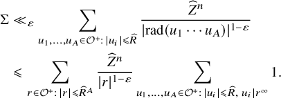
Lemma 2.2 now yields

from which the statement follows on redefining
$\varepsilon $
 .
.
At several points later, we shall require nontrivial bounds on certain level sets. Let
$\overline {K}$
 denote the algebraic closure of K. For each place v of K, fix an embedding of
$\overline {K}$
denote the algebraic closure of K. For each place v of K, fix an embedding of
$\overline {K}$
 into the algebraic closure
$\overline {K}_v$
into the algebraic closure
$\overline {K}_v$
 of
$K_v$
of
$K_v$
 . The absolute value
$\lvert \cdot \rvert _v$
. The absolute value
$\lvert \cdot \rvert _v$
 on
$K_v$
on
$K_v$
 extends uniquely to
$\overline {K}_v$
extends uniquely to
$\overline {K}_v$
 . Restricting from
$\overline {K}_v$
. Restricting from
$\overline {K}_v$
 to
$\overline {K}$
to
$\overline {K}$
 , we thus obtain an absolute value
$\lvert \cdot \rvert _v$
, we thus obtain an absolute value
$\lvert \cdot \rvert _v$
 on
$\overline {K}$
on
$\overline {K}$
 .
.
Lemma 2.4. Let
$B,\lambda \in \mathbb {R}$
 and
$z\in \overline {K}$
and
$z\in \overline {K}$
 . Uniformly over places v of K, we have

Proof. This is trivial if
$v=\infty $
 . If
$v=\varpi \ne \infty $
. If
$v=\varpi \ne \infty $
 , we write
$\Omega _z$
, we write
$\Omega _z$
 for the set appearing on the left hand side, which we may assume is nonempty. Fix an element
$x_0\in \Omega _z$
for the set appearing on the left hand side, which we may assume is nonempty. Fix an element
$x_0\in \Omega _z$
 and note that
$\lvert x-z \rvert _v \leqslant \widehat \lambda \Leftrightarrow \lvert x-x_0 \rvert _v \leqslant \widehat \lambda \Leftrightarrow \varpi ^l \mid x-x_0$
and note that
$\lvert x-z \rvert _v \leqslant \widehat \lambda \Leftrightarrow \lvert x-x_0 \rvert _v \leqslant \widehat \lambda \Leftrightarrow \varpi ^l \mid x-x_0$
 , where
$l := -\lfloor \lambda /\deg {\varpi } \rfloor \in \mathbb {Z}$
, where
$l := -\lfloor \lambda /\deg {\varpi } \rfloor \in \mathbb {Z}$
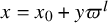
 . Hence we can write
$x = x_0+y\varpi ^l$
. Hence we can write
$x = x_0+y\varpi ^l$
 with
$y\in \mathcal {O}$
with
$y\in \mathcal {O}$
 , to get

where
$z_0 := -x_0/\varpi ^l\in K$
 . By the ‘
$v=\infty $
. By the ‘
$v=\infty $
 case’ of (2.19), the desired result follows, since
$\widehat B/\lvert \varpi \rvert ^l = \widehat B/q^{l\deg {\varpi }} = \widehat B q^{(\deg {\varpi }) \lfloor \lambda /\deg {\varpi } \rfloor } \leqslant \widehat B \widehat \lambda $
case’ of (2.19), the desired result follows, since
$\widehat B/\lvert \varpi \rvert ^l = \widehat B/q^{l\deg {\varpi }} = \widehat B q^{(\deg {\varpi }) \lfloor \lambda /\deg {\varpi } \rfloor } \leqslant \widehat B \widehat \lambda $
 .
.
Lemma 2.5. Suppose
$f\in K[x]$
 has leading term
$ax^d$
has leading term
$ax^d$
 with
$a\neq 0$
with
$a\neq 0$
 and
$d\geqslant 1$
and
$d\geqslant 1$
 . Let
$B,\lambda \in \mathbb {R}$
. Let
$B,\lambda \in \mathbb {R}$
 . Then, uniformly over places v of K, we have

Proof. We use the idea behind Lemma 1 of [Reference Browning, Heath-Brown and Salberger10]. By replacing f with
$f/a$
 , we may assume f is monic. Let
$z_1,\dots ,z_d\in \overline {K}$
, we may assume f is monic. Let
$z_1,\dots ,z_d\in \overline {K}$
 be the roots of f. Then

Summing (2.19) over
$z=z_i$
 gives the desired result.
Given
$f\in \mathcal {O}[x]$
 and
$r\in \mathcal {O}^+$
and
$r\in \mathcal {O}^+$
 , let
$N(f;r)$
, let
$N(f;r)$
 be the number of solutions
$x\in \mathcal {O}/r\mathcal {O}$
be the number of solutions
$x\in \mathcal {O}/r\mathcal {O}$
 to
$f(x)\equiv 0\bmod {r}$
to
$f(x)\equiv 0\bmod {r}$
 . Similarly, for
$g\in \mathcal {O}[y_1,\dots ,y_n]$
. Similarly, for
$g\in \mathcal {O}[y_1,\dots ,y_n]$
 , define

Lemma 2.6. Suppose
$f\in \mathcal {O}[x]$
 has leading term
$ax^d$
has leading term
$ax^d$
 with
$a\neq 0$
with
$a\neq 0$
 and
$d\geqslant 1$
and
$d\geqslant 1$
 . Then there exists
$A_d>0$
. Then there exists
$A_d>0$
 such that for any
$r\in \mathcal {O}^+$
such that for any
$r\in \mathcal {O}^+$
 we have

Moreover, if r is square-free then

Proof. By the Chinese remainder theorem it suffices to assume
$r=\varpi ^l$
 is a prime power. Next, observe that
$N(f;r) = N(f+rx^d;r)$
is a prime power. Next, observe that
$N(f;r) = N(f+rx^d;r)$
 and
$\min (v_\varpi (a),v_\varpi (a+r))\leqslant v_\varpi (r)$
and
$\min (v_\varpi (a),v_\varpi (a+r))\leqslant v_\varpi (r)$
 . Therefore, after possibly replacing f with
$f+rx^d$
. Therefore, after possibly replacing f with
$f+rx^d$
 , we may assume that
$a\mid r$
, we may assume that
$a\mid r$
 . Then to get (2.22), we apply (2.20) with
$ (\widehat B,\widehat \lambda ,v) = (\lvert r \rvert ,\lvert r \rvert ^{-1},\varpi )$
. Then to get (2.22), we apply (2.20) with
$ (\widehat B,\widehat \lambda ,v) = (\lvert r \rvert ,\lvert r \rvert ^{-1},\varpi )$
 , noting that
$|a|_\varpi ^{-1}=q^{v_\varpi (a)} = |a| = \lvert \gcd (r,a) \rvert $
, noting that
$|a|_\varpi ^{-1}=q^{v_\varpi (a)} = |a| = \lvert \gcd (r,a) \rvert $
 . Moreover, if
$l=1$
. Moreover, if
$l=1$
 , then (2.23) holds because
$N(f;\varpi ) \leqslant d\, \lvert \gcd (\varpi ,a) \rvert $
, then (2.23) holds because
$N(f;\varpi ) \leqslant d\, \lvert \gcd (\varpi ,a) \rvert $
 .
.
Before stating a useful consequence of this result, we first prove a technical result which allows us to make a convenient change of variables.
Lemma 2.7. Let
$n\geqslant 1$
 . Let S be a finite subset of
$\mathcal {O}[y_1,\dots ,y_n] \setminus \{0\}$
. Let S be a finite subset of
$\mathcal {O}[y_1,\dots ,y_n] \setminus \{0\}$
 . Then there exists
$\boldsymbol {a}=(a_2,\dots ,a_n)\in \mathcal {O}^{n-1}$
. Then there exists
$\boldsymbol {a}=(a_2,\dots ,a_n)\in \mathcal {O}^{n-1}$
 such that for all
$g\in S$
such that for all
$g\in S$
 , we have

where
$\boldsymbol {a}^\ast {g} := g(y_1,y_2+a_2y_1,\dots ,y_n+a_ny_1)\in \mathcal {O}[y_1,\dots ,y_n]$
 .
.
Proof. For each
$g\in S$
 , let
$h_g\in \mathcal {O}[y_1,\dots ,y_n]\setminus \{0\}$
, let
$h_g\in \mathcal {O}[y_1,\dots ,y_n]\setminus \{0\}$
 be the leading homogeneous part of g, so that
$\deg {h_g} = \deg {g}$
be the leading homogeneous part of g, so that
$\deg {h_g} = \deg {g}$
 and
$\deg (g-h_g) < \deg {g}$
and
$\deg (g-h_g) < \deg {g}$
 . Then for any
$g\in S$
. Then for any
$g\in S$
 and
$\boldsymbol {a}\in R^{n-1}$
and
$\boldsymbol {a}\in R^{n-1}$
 (for any K-algebra R), the desired property is equivalent to

But
$h_g$
 is homogeneous, so this defines a nonempty open subscheme of
$\mathbb {A}^{n-1}_K$
is homogeneous, so this defines a nonempty open subscheme of
$\mathbb {A}^{n-1}_K$
 . Since S is finite and
$\mathcal {O}^{n-1}$
. Since S is finite and
$\mathcal {O}^{n-1}$
 is Zariski dense in
$\mathbb {A}^{n-1}_K$
is Zariski dense in
$\mathbb {A}^{n-1}_K$
 , the lemma follows.
Corollary 2.8. Fix a nonconstant polynomial
$g\in \mathcal {O}[y_1,\dots ,y_n]$
 , where
$n\geqslant 1$
, where
$n\geqslant 1$
 . Then there exists
$A_g>0$
. Then there exists
$A_g>0$
 such that for any
$r\in \mathcal {O}^+$
such that for any
$r\in \mathcal {O}^+$
 we have

Proof. This is analogous to [Reference Pierce, Schindler and Wood44, Lemma 4.10] (in which the homogeneity assumed is unimportant). By Lemma 2.7, we can make an
$\mathcal {O}$
 -linear change of variables in order to assume that
$\deg _{y_1}(g) = \deg (g)$
-linear change of variables in order to assume that
$\deg _{y_1}(g) = \deg (g)$
 . Then (2.22) immediately implies the desired bound.
Beyond Corollary 2.8, we need a strong estimate for square-free polynomials.
Lemma 2.9. Fix a nonzero polynomial
$g\in \mathcal {O}[y_1,\dots ,y_n]$
 , where
$n\geqslant 1$
, where
$n\geqslant 1$
 . Assume g is square-free as an element of
$K[y_1,\dots ,y_n]$
. Assume g is square-free as an element of
$K[y_1,\dots ,y_n]$
 . Then there exists
$A_g>0$
. Then there exists
$A_g>0$
 such that for all cube-free
$r\in \mathcal {O}^+$
such that for all cube-free
$r\in \mathcal {O}^+$
 we have

Proof. Assume
$r=\varpi ^l$
 . When
$l=1$
. When
$l=1$
 , the Lang–Weil estimate for the quasi-projective variety
$g=0$
, the Lang–Weil estimate for the quasi-projective variety
$g=0$
 implies
$N(g;\varpi ) \ll _g \lvert \varpi \rvert ^{n-1}=\lvert r \rvert ^{n-1}$
implies
$N(g;\varpi ) \ll _g \lvert \varpi \rvert ^{n-1}=\lvert r \rvert ^{n-1}$
 . When
$l=2$
. When
$l=2$
 , care is needed because K is not perfect. Nonetheless, in [Reference Poonen45, final paragraph of § 7 (in “Proof of Theorem 3.4”)], it is shown that
$N(g;\varpi ^2) \ll _g \lvert \varpi \rvert ^{2n-2} = \lvert r \rvert ^{n-1}$
, care is needed because K is not perfect. Nonetheless, in [Reference Poonen45, final paragraph of § 7 (in “Proof of Theorem 3.4”)], it is shown that
$N(g;\varpi ^2) \ll _g \lvert \varpi \rvert ^{2n-2} = \lvert r \rvert ^{n-1}$
 . This completes the proof.
Finally, we need an affine dimension growth bound available from [Reference Browning and Vishe12].
Lemma 2.10 [Reference Browning and Vishe12, Lemma 2.8]
Let
$B\geqslant 0$
 . Any affine K-variety W (equipped with an integral model over
$\mathcal {O}$
. Any affine K-variety W (equipped with an integral model over
$\mathcal {O}$
 ) satisfies
$\#\{\boldsymbol {y}\in W(\mathcal {O}): \lvert \boldsymbol {y} \rvert \leqslant \widehat B\} \ll _W {\widehat B}^{\dim {W}}$
) satisfies
$\#\{\boldsymbol {y}\in W(\mathcal {O}): \lvert \boldsymbol {y} \rvert \leqslant \widehat B\} \ll _W {\widehat B}^{\dim {W}}$
 .
.
3 Ratios Conjecture and applications
We start generally and then specialise. Let
$K^{\text {sep}}$
 be the separable closure of K. Fix a prime
$\ell \ne \operatorname {\mathrm {char}}(\mathbb {F}_q)$
be the separable closure of K. Fix a prime
$\ell \ne \operatorname {\mathrm {char}}(\mathbb {F}_q)$
 . For a smooth proper K-variety X, define the
$\ell $
. For a smooth proper K-variety X, define the
$\ell $
 -adic cohomology

This is an
$\ell $
 -adic representation of
$\operatorname {\mathrm {Gal}}(K^{\text {sep}}/K)$
-adic representation of
$\operatorname {\mathrm {Gal}}(K^{\text {sep}}/K)$
 , pure of weight i by Deligne’s resolution of the Weil Conjectures [Reference Deligne20]. The exterior square representation
$\bigwedge ^2{H^i_\ell (X)}$
, pure of weight i by Deligne’s resolution of the Weil Conjectures [Reference Deligne20]. The exterior square representation
$\bigwedge ^2{H^i_\ell (X)}$
 , which will soon play an important role, is pure of weight
$2i$
, which will soon play an important role, is pure of weight
$2i$
 .
.
In general, for an
$\ell $
 -adic representationFootnote
1
M of
$\operatorname {\mathrm {Gal}}(K^{\text {sep}}/K)$
-adic representationFootnote
1
M of
$\operatorname {\mathrm {Gal}}(K^{\text {sep}}/K)$
 , pure of weight
$w\in \mathbb {Z}$
, pure of weight
$w\in \mathbb {Z}$
 , we make the following definitions.
-
1. Let $M^{I_v}$
be the inertia invariants of M at v. Let
$\alpha ^0_{M,j}(v)$
(for
$1\leqslant j\leqslant \dim {M^{I_v}}$
) be the eigenvalues of geometric Frobenius on
$M^{I_v}$
. -
2. Let $\alpha _{M,j}(v) := \alpha ^0_{M,j}(v) / (\# k_v)^{w/2}$
, where
$k_v$
is the residue field of
$\mathcal {O}_v$
. -
3. Let
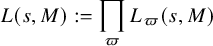
$$ \begin{align*}L_v(s,M) := \prod_j (1-\alpha_{M,j}(v)\lvert k_v \rvert^{-s})^{-1}\end{align*} $$be the analytically normalised local factor at v. Let
$$ \begin{align*}L(s,M) := \prod_{\varpi} L_\varpi(s,M)\end{align*} $$(with $\varpi \ne \infty $
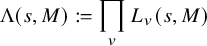
) and $$ \begin{align*}\Lambda(s,M) := \prod_v L_v(s,M)\end{align*} $$(including $v=\infty $
), so that
$\Lambda (\ast ) = L(\ast ) L_\infty (\ast )$
.











Let V and
$V_{\boldsymbol {c}}$
 be the K-varieties in
$\mathbb {P}^{5}_K$
be the K-varieties in
$\mathbb {P}^{5}_K$
 defined by
$F(\boldsymbol {x})=0$
defined by
$F(\boldsymbol {x})=0$
 and
$F(\boldsymbol {x})=\boldsymbol {c}\cdot \boldsymbol {x}=0$
and
$F(\boldsymbol {x})=\boldsymbol {c}\cdot \boldsymbol {x}=0$
 , respectively. Let
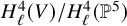
$L(s,V) = L(s,H^4_\ell (V)/H^4_\ell (\mathbb {P}^5))$
, respectively. Let
$L(s,V) = L(s,H^4_\ell (V)/H^4_\ell (\mathbb {P}^5))$
 , and for
$\boldsymbol {c}\in \mathcal {S}_1$
, and for
$\boldsymbol {c}\in \mathcal {S}_1$
 let
let

Let
$\alpha _{V,j}(v)$
 ,
$\alpha _{\boldsymbol {c},j}(v)$
,
$\alpha _{\boldsymbol {c},j}(v)$
 ,
$\alpha _{\boldsymbol {c},\bigwedge ^2,j}(v)$
,
$\alpha _{\boldsymbol {c},\bigwedge ^2,j}(v)$
 be the corresponding normalised eigenvalues. The local factors are independent of
$\ell $
be the corresponding normalised eigenvalues. The local factors are independent of
$\ell $
 , by [Reference Kahn35, Theorem 5.46], and the number of normalised eigenvalues in each case is
$\leqslant \binom {10}{2}=45$
, by [Reference Kahn35, Theorem 5.46], and the number of normalised eigenvalues in each case is
$\leqslant \binom {10}{2}=45$
 , by classical Betti number calculations for smooth projective hypersurfaces over
$\mathbb {C}$
, by classical Betti number calculations for smooth projective hypersurfaces over
$\mathbb {C}$
 , which follow for instance from [Reference Arapura3, Corollary 17.3.8].
For
$r\in \mathcal {O}^+$
 , define
$\lambda _V(r)$
, define
$\lambda _V(r)$
 ,
$\lambda _{\boldsymbol {c}}(r)$
,
$\lambda _{\boldsymbol {c}}(r)$
 ,
$\lambda _{\boldsymbol {c},\bigwedge ^2}(r)$
,
$\lambda _{\boldsymbol {c},\bigwedge ^2}(r)$
 to be the rth coefficients of the Euler products
$L(s,V)$
to be the rth coefficients of the Euler products
$L(s,V)$
 ,
$L(s,\boldsymbol {c})$
,
$L(s,\boldsymbol {c})$
 ,
$L(s,\boldsymbol {c},\bigwedge ^2)$
,
$L(s,\boldsymbol {c},\bigwedge ^2)$
 , respectively. More precisely, for prime
$\varpi \in \mathcal {O}^+$
, respectively. More precisely, for prime
$\varpi \in \mathcal {O}^+$
 let
$\lambda _\ast (\varpi ^k)$
let
$\lambda _\ast (\varpi ^k)$
 be the coefficient of
$\lvert \varpi \rvert ^{-ks}$
be the coefficient of
$\lvert \varpi \rvert ^{-ks}$
 in
$L_\varpi (s,\ast )$
in
$L_\varpi (s,\ast )$
 , and extend multiplicatively to define
$\lambda _\ast (r)$
, and extend multiplicatively to define
$\lambda _\ast (r)$
 for
$r\in \mathcal {O}^+$
for
$r\in \mathcal {O}^+$
 . (We have to carefully define
$\lambda _\ast (r)$
. (We have to carefully define
$\lambda _\ast (r)$
 , because for any
$\varpi $
, because for any
$\varpi $
 ,
$\varpi '$
,
$\varpi '$
 the sizes
$\lvert \varpi \rvert $
the sizes
$\lvert \varpi \rvert $
 ,
$\lvert \varpi ' \rvert $
,
$\lvert \varpi ' \rvert $
 are multiplicatively dependent.)
Let
$\mathsf {T} = \frac {2\pi }{\log {q}}$
 . Note that
$q^s$
. Note that
$q^s$
 is invariant under translation by
$i\mathsf {T}$
is invariant under translation by
$i\mathsf {T}$
 , so
, so

Let
$\zeta _K(s) := \prod _{\varpi } (1 - \lvert \varpi \rvert ^{-s})^{-1} = \sum _{r\in \mathcal {O}^+} \lvert r \rvert ^{-s} = (1-q^{1-s})^{-1}$
 . For later convenience we define

and
$L_v(s,\boldsymbol {c},2) := L_v(s,\boldsymbol {c},{\textstyle \bigwedge ^2})/\zeta _{K,v}(s)$
 .
.
Proposition 3.1. Let
$\boldsymbol {c}\in \mathcal {S}_1$
 . Let
$L(s)$
. Let
$L(s)$
 be one of
$\zeta _K(s)$
be one of
$\zeta _K(s)$
 ,
$L(s,V)$
,
$L(s,V)$
 ,
$L(s,\boldsymbol {c})$
,
$L(s,\boldsymbol {c})$
 ,
$L(s,\boldsymbol {c},\bigwedge ^2)$
,
$L(s,\boldsymbol {c},\bigwedge ^2)$
 ,
$L(s,\boldsymbol {c},2)$
,
$L(s,\boldsymbol {c},2)$
 . Let
$\Lambda (s) = L(s) L_\infty (s)$
. Let
$\Lambda (s) = L(s) L_\infty (s)$
 be the corresponding completed L-function.
-
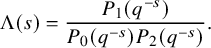
1. There exist unique polynomials $P_0,P_1,P_2\in 1+z\,\mathbb {R}[z]$
, where the roots of
$P_i$
are complex numbers of size
$q^{-i/2}$
, such that $$ \begin{align*} \Lambda(s) = \frac{P_1(q^{-s})}{P_0(q^{-s}) P_2(q^{-s})}. \end{align*} $$
-
2. $\deg {P_0},\deg {P_2} \ll 1$
and
$\deg {P_1} \ll 1+\log \lvert F^\ast (\boldsymbol {c}) \rvert $
. -
3. At each place v, the local factor $L_v(s) = \prod _\alpha (1-\alpha q^{-s})^{-1}$
has real coefficients, and the inverse roots
$\alpha $
satisfy the Ramanujan bound
$\lvert \alpha \rvert \leqslant 1$
. -
4. We have $1/L(s) \ll _{\varepsilon } \lvert \boldsymbol {c} \rvert ^\varepsilon $
for
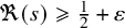
$\Re (s)\geqslant \frac 12+\varepsilon $
. -
5. The $\widehat R^{-s}$
coefficient of
$1/L(s)\in \mathbb {R}[[q^{-s}]]$
is
$\ll _{\varepsilon } \lvert \boldsymbol {c} \rvert ^\varepsilon \widehat R^{1/2+\varepsilon }$
for all
$R\in \mathbb {Z}_{\geqslant 0}$
.













Proof. (1): For
$\zeta _K(s)$
 ,
$L(s,V)$
,
$L(s,V)$
 ,
$L(s,\boldsymbol {c})$
,
$L(s,\boldsymbol {c})$
 ,
$L(s,\boldsymbol {c},\bigwedge ^2)$
,
$L(s,\boldsymbol {c},\bigwedge ^2)$
 , this follows directly from [Reference Kahn35, proof of Theorem 5.58], since the corresponding
$\ell $
, this follows directly from [Reference Kahn35, proof of Theorem 5.58], since the corresponding
$\ell $
 -adic sheaves
$\mathbb {Q}_\ell $
-adic sheaves
$\mathbb {Q}_\ell $
 ,
$H^4_\ell (V)/H^4_\ell (\mathbb {P}^5)$
,
$H^4_\ell (V)/H^4_\ell (\mathbb {P}^5)$
 ,
$H^3_\ell (V_{\boldsymbol {c}})$
,
$H^3_\ell (V_{\boldsymbol {c}})$
 ,
$\bigwedge ^2{H^3_\ell (V_{\boldsymbol {c}})}$
,
$\bigwedge ^2{H^3_\ell (V_{\boldsymbol {c}})}$
 are ‘weakly polarisable’ (by Poincaré duality on V and
$V_{\boldsymbol {c}}$
are ‘weakly polarisable’ (by Poincaré duality on V and
$V_{\boldsymbol {c}}$
 , which gives a symmetric pairing on
$H^4_\ell (V)$
, which gives a symmetric pairing on
$H^4_\ell (V)$
 and a skew-symmetric pairing on
$H^3_\ell (V_{\boldsymbol {c}})$
and a skew-symmetric pairing on
$H^3_\ell (V_{\boldsymbol {c}})$
 , and thus a symmetric pairing on the tensor squares thereof). By Proposition 3.2 and the formula
$\zeta _K(s) = 1/(1-q^{1-s})$
, and thus a symmetric pairing on the tensor squares thereof). By Proposition 3.2 and the formula
$\zeta _K(s) = 1/(1-q^{1-s})$
 , the result then follows for
$L(s,\boldsymbol {c},2)$
, the result then follows for
$L(s,\boldsymbol {c},2)$
 by (3.2).
(2): This is explained in [Reference Browning and Vishe12, § 3.4] using Swan conductors.
(3): This follows from [Reference Kahn35, Theorem 5.46].
(4): This follows from (1)–(3) and the Hadamard three circle theorem as in [Reference Browning and Vishe12, proof of Lemma 8.4].
(5): Let
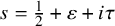
$s=\frac 12+\varepsilon +i\tau $
 and integrate
$\widehat R^s/L(s) \ll _{\varepsilon } \lvert \boldsymbol {c} \rvert ^\varepsilon \widehat R^{1/2+\varepsilon }$
and integrate
$\widehat R^s/L(s) \ll _{\varepsilon } \lvert \boldsymbol {c} \rvert ^\varepsilon \widehat R^{1/2+\varepsilon }$
 over
$\tau \in \mathbb {R}/\mathsf {T}\mathbb {Z}$
over
$\tau \in \mathbb {R}/\mathsf {T}\mathbb {Z}$
 .
.
Proposition 3.2. Let
$\boldsymbol {c}\in \mathcal {S}_1$
 . Then
$L(s,\boldsymbol {c},\bigwedge ^2)$
. Then
$L(s,\boldsymbol {c},\bigwedge ^2)$
 has a pole at
$s=1$
has a pole at
$s=1$
 .
.
Proof. Let
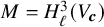
$M = H^3_\ell (V_{\boldsymbol {c}})$
 . Poincaré duality gives a perfect skew-symmetric pairing

where
$\mathbb {Q}_\ell (-3)$
 denotes the Tate motive of weight
$6$
denotes the Tate motive of weight
$6$
 . Since
$\psi $
. Since
$\psi $
 is surjective, its dual

is injective. But
$\psi $
 is perfect, so that it induces an isomorphism

After twisting
$\psi ^\vee $
 by
$\mathbb {Q}_\ell (-6)$
by
$\mathbb {Q}_\ell (-6)$
 , we thus obtain an injection
$\mathbb {Q}_\ell (-3) \to M \wedge M$
, we thus obtain an injection
$\mathbb {Q}_\ell (-3) \to M \wedge M$
 . Thus
$(M\wedge M)(3)$
. Thus
$(M\wedge M)(3)$
 (which is pure of weight
$0$
(which is pure of weight
$0$
 ) has a nonzero space of
$\operatorname {\mathrm {Gal}}(K^{\text {sep}}/K)$
) has a nonzero space of
$\operatorname {\mathrm {Gal}}(K^{\text {sep}}/K)$
 -invariants. So by [Reference Lyons42, correction to Theorem 2.1] (which builds on [Reference Lafforgue40,Reference Lyons41]), it follows that the L-function
$L(s,(M\wedge M)(3)) = L(s,\boldsymbol {c},\textstyle {\bigwedge ^2})$
-invariants. So by [Reference Lyons42, correction to Theorem 2.1] (which builds on [Reference Lafforgue40,Reference Lyons41]), it follows that the L-function
$L(s,(M\wedge M)(3)) = L(s,\boldsymbol {c},\textstyle {\bigwedge ^2})$
 has a pole at
$s=1$
has a pole at
$s=1$
 .
.
Proposition 3.3 (Kisin)
Fix a prime
$\varpi \in \mathcal {O}^+$
 and a tuple
$\boldsymbol {b}\in \mathcal {O}_\varpi ^6$
and a tuple
$\boldsymbol {b}\in \mathcal {O}_\varpi ^6$
 with
$F^\ast (\boldsymbol {b})\ne 0$
with
$F^\ast (\boldsymbol {b})\ne 0$
 . Then there exists an integer
$l\geqslant 0$
. Then there exists an integer
$l\geqslant 0$
 , depending only on
$\varpi $
, depending only on
$\varpi $
 and
$\boldsymbol {b}$
and
$\boldsymbol {b}$
 , such that for all tuples
$\boldsymbol {a}\in \mathcal {O}_\varpi ^6$
, such that for all tuples
$\boldsymbol {a}\in \mathcal {O}_\varpi ^6$
 with
$\boldsymbol {a}\equiv \boldsymbol {b}\bmod {\varpi ^{1+l}}$
with
$\boldsymbol {a}\equiv \boldsymbol {b}\bmod {\varpi ^{1+l}}$
 , we have
$F^\ast (\boldsymbol {a})\ne 0$
, we have
$F^\ast (\boldsymbol {a})\ne 0$
 and
$L_\varpi (s,\boldsymbol {a}) = L_\varpi (s,\boldsymbol {b})$
and
$L_\varpi (s,\boldsymbol {a}) = L_\varpi (s,\boldsymbol {b})$
 .
.
Proof. This follows directly from [Reference Kisin37, case (2) of Theorem 5.1].
Lemma 3.4. For each
$\boldsymbol {b}\in \mathcal {O}_\varpi ^6$
 with
$F^\ast (\boldsymbol {b})\ne 0$
with
$F^\ast (\boldsymbol {b})\ne 0$
 , let
$l(\varpi ,\boldsymbol {b})$
, let
$l(\varpi ,\boldsymbol {b})$
 be the smallest integer
$l\geqslant 0$
be the smallest integer
$l\geqslant 0$
 verifying Proposition 3.3. Then for any integer
$l\geqslant 0$
verifying Proposition 3.3. Then for any integer
$l\geqslant 0$
 , the set

is closed under translation by
$\varpi ^{l+1}\mathcal {O}_\varpi ^6$
 , and its measure tends to
$1$
, and its measure tends to
$1$
 as
$l\to \infty $
as
$l\to \infty $
 .
.
Proof. We first show that
$l(\varpi ,\boldsymbol {b})$
 is locally constant. Let
$\boldsymbol {b}, \boldsymbol {c}\in \mathcal {O}_\varpi ^6$
is locally constant. Let
$\boldsymbol {b}, \boldsymbol {c}\in \mathcal {O}_\varpi ^6$
 with
$F^\ast (\boldsymbol {b})\ne 0$
with
$F^\ast (\boldsymbol {b})\ne 0$
 and
$\boldsymbol {c}\equiv \boldsymbol {b}\bmod {\varpi ^{1+l(\varpi ,\boldsymbol {b})}}$
and
$\boldsymbol {c}\equiv \boldsymbol {b}\bmod {\varpi ^{1+l(\varpi ,\boldsymbol {b})}}$
 . Then
$F^\ast (\boldsymbol {c})\ne 0$
. Then
$F^\ast (\boldsymbol {c})\ne 0$
 and
$L_\varpi (s, \boldsymbol {c}) = L_\varpi (s, \boldsymbol {b})$
and
$L_\varpi (s, \boldsymbol {c}) = L_\varpi (s, \boldsymbol {b})$
 , and thus
$l(\varpi ,\boldsymbol {c})\leqslant l(\varpi ,\boldsymbol {b})$
, and thus
$l(\varpi ,\boldsymbol {c})\leqslant l(\varpi ,\boldsymbol {b})$
 (since
$\boldsymbol {a}\equiv \boldsymbol {c}\bmod {\varpi ^{1+l(\varpi ,\boldsymbol {b})}} \Rightarrow \boldsymbol {a}\equiv \boldsymbol {b}\bmod {\varpi ^{1+l(\varpi ,\boldsymbol {b})}}$
(since
$\boldsymbol {a}\equiv \boldsymbol {c}\bmod {\varpi ^{1+l(\varpi ,\boldsymbol {b})}} \Rightarrow \boldsymbol {a}\equiv \boldsymbol {b}\bmod {\varpi ^{1+l(\varpi ,\boldsymbol {b})}}$
 ). But then
$\boldsymbol {b}\equiv \boldsymbol {c}\bmod {\varpi ^{1+l(\varpi ,\boldsymbol {c})}}$
). But then
$\boldsymbol {b}\equiv \boldsymbol {c}\bmod {\varpi ^{1+l(\varpi ,\boldsymbol {c})}}$
 , so
$l(\varpi ,\boldsymbol {b})\leqslant l(\varpi ,\boldsymbol {c})$
, so
$l(\varpi ,\boldsymbol {b})\leqslant l(\varpi ,\boldsymbol {c})$
 , whence
$l(\varpi ,\boldsymbol {b}) = l(\varpi ,\boldsymbol {c})$
, whence
$l(\varpi ,\boldsymbol {b}) = l(\varpi ,\boldsymbol {c})$
 . So if
$\boldsymbol {b}$
. So if
$\boldsymbol {b}$
 lies in (3.3) for some
$l\geqslant 0$
lies in (3.3) for some
$l\geqslant 0$
 , then (3.3) is indeed closed under translation by
$\varpi ^{l+1}\mathcal {O}_\varpi ^6$
, then (3.3) is indeed closed under translation by
$\varpi ^{l+1}\mathcal {O}_\varpi ^6$
 .
.
We now turn to measures. Let
$A\in \mathbb {Z}_{\geqslant 0}$
 . The set
$S_A = \{\boldsymbol {c}\in \mathcal {O}_\varpi ^6: v_\varpi (F^\ast (\boldsymbol {c}))\leqslant A\}$
. The set
$S_A = \{\boldsymbol {c}\in \mathcal {O}_\varpi ^6: v_\varpi (F^\ast (\boldsymbol {c}))\leqslant A\}$
 is compact. Yet the function
$\boldsymbol {b}\mapsto l(\varpi ,\boldsymbol {b})$
is compact. Yet the function
$\boldsymbol {b}\mapsto l(\varpi ,\boldsymbol {b})$
 on
$S_A$
on
$S_A$
 is continuous. So (3.3) contains
$S_A$
is continuous. So (3.3) contains
$S_A$
 for all
$l\gg _A 1$
for all
$l\gg _A 1$
 , say. But by Corollary 2.8, the measure of
$S_A$
, say. But by Corollary 2.8, the measure of
$S_A$
 tends to
$1$
tends to
$1$
 as
$A\to \infty $
as
$A\to \infty $
 .
.
Let
$\mu _{\boldsymbol {c}}(r)$
 be the rth coefficient of the Euler product
$L(s,\boldsymbol {c})^{-1} = \prod _\varpi L_\varpi (s,\boldsymbol {c})^{-1}$
be the rth coefficient of the Euler product
$L(s,\boldsymbol {c})^{-1} = \prod _\varpi L_\varpi (s,\boldsymbol {c})^{-1}$
 . The following result collects together some facts about averages of
$\mu _{\boldsymbol {c}}(r)$
. The following result collects together some facts about averages of
$\mu _{\boldsymbol {c}}(r)$
 over vectors
$\boldsymbol {c}$
over vectors
$\boldsymbol {c}$
 .
.
Proposition 3.5. Let
$r_1,r_2\in \mathcal {O}^+$
 . Let
$\mathbb {E}_{\boldsymbol {c}\in S}[f]$
. Let
$\mathbb {E}_{\boldsymbol {c}\in S}[f]$
 be the average of f over S. The limit

exists. Moreover,
$\bar {\mu }_{F,2} (r_1,r_2)\bar {\mu }_{F,2}(r^{\prime }_1,r^{\prime }_2) = \bar {\mu }_{F,2}(r_1r^{\prime }_1,r_2r^{\prime }_2) $
 if
$\gcd (r_1r_2,r^{\prime }_1r^{\prime }_2)=1$
if
$\gcd (r_1r_2,r^{\prime }_1r^{\prime }_2)=1$
 .
.
Now let
$\varpi \in \mathcal {O}^+$
 be a prime, and let
$l,l_1,l_2\geqslant 0$
be a prime, and let
$l,l_1,l_2\geqslant 0$
 be integers. Then

Furthermore,


Proof. This result is directly analogous to [Reference Wang57, Proposition 6.1], and is purely local. For the reader’s convenience, we highlight the main points. Existence and multiplicativity of the limit follow from Lemma 3.4, the bound
$\lvert \mu _{\boldsymbol {c}}(r) \rvert \ll _\varepsilon \lvert r \rvert ^\varepsilon $
 (which follows from Proposition 3.1(3)) and the Chinese remainder theorem. The bound
$\lvert \mu _{\boldsymbol {c}}(r) \rvert \ll _\varepsilon \lvert r \rvert ^\varepsilon $
(which follows from Proposition 3.1(3)) and the Chinese remainder theorem. The bound
$\lvert \mu _{\boldsymbol {c}}(r) \rvert \ll _\varepsilon \lvert r \rvert ^\varepsilon $
 implies (3.4). The estimates in (3.5) and (3.6) are subtler; they relate to the rank and homogeneity type [Reference Sarnak, Shin and Templier46, § 1] of our geometric family of L-functions
$L(s,\boldsymbol {c})$
implies (3.4). The estimates in (3.5) and (3.6) are subtler; they relate to the rank and homogeneity type [Reference Sarnak, Shin and Templier46, § 1] of our geometric family of L-functions
$L(s,\boldsymbol {c})$
 .
.
Recall the definition of
$E^\natural _{\boldsymbol {c}}(k)$
 from (2.15). The following hold uniformly over primes
$\varpi \in \mathcal {O}^+$
from (2.15). The following hold uniformly over primes
$\varpi \in \mathcal {O}^+$
 (where
$k_\varpi = \mathcal {O}/\varpi \mathcal {O}$
(where
$k_\varpi = \mathcal {O}/\varpi \mathcal {O}$
 and
$k_{\varpi ,2}$
and
$k_{\varpi ,2}$
 is the unique quadratic field extension of
$k_\varpi $
is the unique quadratic field extension of
$k_\varpi $
 ):
):



This is proven for prime fields in [Reference Wang53, Corollary 1.7]; the proof there carries over directly to arbitrary finite fields of characteristic
$>3$
 .
.
Finally, observe that if
$\varpi \nmid F^\ast (\boldsymbol {c})$
 , then
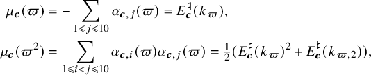
$L_\varpi (s,\boldsymbol {c})^{-1} = \prod _{1\leqslant j\leqslant 10} (1 - \alpha _{\boldsymbol {c},j}(\varpi ) \lvert \varpi \rvert ^{-s})$
, then
$L_\varpi (s,\boldsymbol {c})^{-1} = \prod _{1\leqslant j\leqslant 10} (1 - \alpha _{\boldsymbol {c},j}(\varpi ) \lvert \varpi \rvert ^{-s})$
 , so
, so
because
$E^\natural _{\boldsymbol {c}}(k_\varpi ) = -\sum _{1\leqslant j\leqslant 10} \alpha _{\boldsymbol {c},j}(\varpi )$
 and
$E^\natural _{\boldsymbol {c}}(k_{\varpi ,2}) = -\sum _{1\leqslant j\leqslant 10} \alpha _{\boldsymbol {c},j}(\varpi )^2$
and
$E^\natural _{\boldsymbol {c}}(k_{\varpi ,2}) = -\sum _{1\leqslant j\leqslant 10} \alpha _{\boldsymbol {c},j}(\varpi )^2$
 by the Grothendieck–Lefschetz trace formula. Thus (3.7)–(3.9) imply (3.5) and (3.6).
Informally, Proposition 3.5 tells us

where the terms indexed by
$1\leqslant j\leqslant 2$
 arise from (3.5) and the trivial symmetry identity
$\bar {\mu }_{F,2}(\varpi ^l,1) = \bar {\mu }_{F,2}(1,\varpi ^l)$
arise from (3.5) and the trivial symmetry identity
$\bar {\mu }_{F,2}(\varpi ^l,1) = \bar {\mu }_{F,2}(1,\varpi ^l)$
 . Motivated by this, let

which by Proposition 3.5 converges absolutely for
$\Re (s_1), \Re (s_2)> \frac 13$
 . The expression
$A_{F,2}$
. The expression
$A_{F,2}$
 appears as the ‘leading constant’ in the Ratios Conjecture for
Let
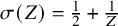
$\sigma (Z) = \frac 12+\frac 1Z$
 . For
$\boldsymbol {c}\in \mathcal {S}_1$
. For
$\boldsymbol {c}\in \mathcal {S}_1$
 , let
, let

For convenience, let
$a_{\boldsymbol {c},1}(r)$
 be the rth coefficient of the Euler product
$\Phi ^{\boldsymbol {c},1}(s)$
be the rth coefficient of the Euler product
$\Phi ^{\boldsymbol {c},1}(s)$
 .
.
The Ratios Recipe [Reference Conrey, Farmer and Zirnbauer17, § 5.1], directly adapted to function fields as in [Reference Andrade and Keating2], produces the following Ratios Conjecture (R2), even with a power-saving error term
$O(\widehat Z^{-\delta })$
 independent of
$\beta $
independent of
$\beta $
 for
$\beta \leqslant \delta $
for
$\beta \leqslant \delta $
 , say. The derivation over K is exactly the same as the derivation over
$\mathbb {Q}$
, say. The derivation over K is exactly the same as the derivation over
$\mathbb {Q}$
 in [Reference Wang57, § 6.3]. We emphasise that the summand on the right-hand side of (3.10) does not depend on
$\boldsymbol {c}$
in [Reference Wang57, § 6.3]. We emphasise that the summand on the right-hand side of (3.10) does not depend on
$\boldsymbol {c}$
 ; a similar point is made after [Reference Wang57, Conjecture 1.5]. For additional context on random matrix predictions for L-functions, we note that the L-functions
$L(s,\boldsymbol {c})$
; a similar point is made after [Reference Wang57, Conjecture 1.5]. For additional context on random matrix predictions for L-functions, we note that the L-functions
$L(s,\boldsymbol {c})$
 over
$\boldsymbol {c}\in \mathcal {S}_1$
over
$\boldsymbol {c}\in \mathcal {S}_1$
 form a geometric family in the sense of [Reference Sarnak, Shin and Templier46, pp. 534–535].
Conjecture 3.6 (R2)
There exists a constant
$\beta \in [0,1]$
 such that if

then uniformly over
$Z\in \mathbb {N}$
 and
$\tau _1,\tau _2\in \mathbb {R}$
and
$\tau _1,\tau _2\in \mathbb {R}$
 , we have

(In fact one would expect (R2) to hold with
$\beta =0$
 , but the approach of [Reference Bergström, Diaconu, Petersen and Westerland5,Reference Miller, Patzt, Petersen and Randal-Williams43] suggests that a small positive value of
$\beta $
, but the approach of [Reference Bergström, Diaconu, Petersen and Westerland5,Reference Miller, Patzt, Petersen and Randal-Williams43] suggests that a small positive value of
$\beta $
 might be more tractable, at least for large fixed q. Also, the ‘slope’
$6$
might be more tractable, at least for large fixed q. Also, the ‘slope’
$6$
 in the exponent
$6\beta $
in the exponent
$6\beta $
 is what we need for our application to Conjecture 3.7 below, but arbitrarily large slope should be permissible.)
For a vertically
$\mathsf {T}$
 -periodic function
$f(s)=f(\sigma +i\tau )$
-periodic function
$f(s)=f(\sigma +i\tau )$
 , define the vertical average

Note that if f is holomorphic on a vertical strip
$\Re (s)\in I$
 , then
$\mathbb {E}_{\Re (s)=\sigma }[f(s)]$
, then
$\mathbb {E}_{\Re (s)=\sigma }[f(s)]$
 is independent of
$\sigma \in I$
is independent of
$\sigma \in I$
 , by Cauchy’s integral theorem over rectangles of height
$\mathsf {T}$
, by Cauchy’s integral theorem over rectangles of height
$\mathsf {T}$
 .
.
Conjecture 3.7. Let
$Z,R\in \mathbb {Z}$
 with
$R\leqslant 3Z$
with
$R\leqslant 3Z$
 . If
$\sigma _0> 1/2$
. If
$\sigma _0> 1/2$
 , then

Proof assuming (R2)
By (3.1) and GRH, the left-hand side of (3.11) is independent of
$\sigma _0>\frac 12$
 . If
$\widehat Z\ll 1$
. If
$\widehat Z\ll 1$
 then (3.11) is trivial, so suppose
$Z\geqslant 2$
then (3.11) is trivial, so suppose
$Z\geqslant 2$
 . We find, after shifting contours to
$\Re (s) = \beta +\sigma (Z)\in (\tfrac 12, 2]$
. We find, after shifting contours to
$\Re (s) = \beta +\sigma (Z)\in (\tfrac 12, 2]$
 and expanding squares using self-duality of
$\Phi ^{\boldsymbol {c},1}$
and expanding squares using self-duality of
$\Phi ^{\boldsymbol {c},1}$
 , the left-hand side of (3.11) equals

After switching the order of
$\boldsymbol {c}$
 and
$\boldsymbol {s}$
and
$\boldsymbol {s}$
 in
$\Sigma_0 $
in
$\Sigma_0 $
 , and plugging in (3.10) for each
$\boldsymbol {s}$
, and plugging in (3.10) for each
$\boldsymbol {s}$
 , we get

where
$\Sigma_1 := \mathbb {E}_{\Re (s)=\beta +\sigma (Z)}[\lvert \widehat R^s \rvert ]=\widehat R^{\beta +\sigma (Z)}$
 and
and

Since
$R\leqslant 3Z$
 and
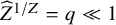
$\widehat {Z}^{1/Z} = q \ll 1$
and
$\widehat {Z}^{1/Z} = q \ll 1$
 , we certainly have
$\Sigma_1 \ll \widehat Z^{3\beta } \widehat R^{1/2}$
, we certainly have
$\Sigma_1 \ll \widehat Z^{3\beta } \widehat R^{1/2}$
 .
.
Let
$\delta =\frac {1}{20}$
 ; then
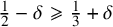
$\frac 12-\delta \geqslant \frac 13+\delta $
; then
$\frac 12-\delta \geqslant \frac 13+\delta $
 . In
$\Sigma_2 $
. In
$\Sigma_2 $
 we shift
$\Re (s_1)$
we shift
$\Re (s_1)$
 from
$\beta +\sigma (Z)$
from
$\beta +\sigma (Z)$
 to
$\frac 12$
to
$\frac 12$
 , then shift
$\Re (s_2)$
, then shift
$\Re (s_2)$
 from
$\beta +\sigma (Z)$
from
$\beta +\sigma (Z)$
 to
$\frac 12-\delta $
to
$\frac 12-\delta $
 . This yields
$\Sigma_2 = \Sigma_3 +O(\Sigma_4 ),$
. This yields
$\Sigma_2 = \Sigma_3 +O(\Sigma_4 ),$
 where
where

comes from the residue
$(\log {q})^{-1}$
 of
$\zeta _K(s_1+s_2) = (1-q^{1-s_1-s_2})^{-1}$
of
$\zeta _K(s_1+s_2) = (1-q^{1-s_1-s_2})^{-1}$
 at
$s_2=1-s_1$
at
$s_2=1-s_1$
 , and where we bound the contribution from
$\Re (s_1) = \frac 12$
, and where we bound the contribution from
$\Re (s_1) = \frac 12$
 and
$\Re (s_2) = \frac 12-\delta $
and
$\Re (s_2) = \frac 12-\delta $
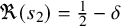 by
by

on using the bounds
$A_{F,2}(s_1,s_2)\ll 1$
 and
$\zeta _K(s_1+s_2)\ll _\delta 1$
and
$\zeta _K(s_1+s_2)\ll _\delta 1$
 . Next we note that

since
$A_{F,2}(s_1, 1-s_1) \ll 1$
 in
$\Sigma_3 $
in
$\Sigma_3 $
 . But
. But

by (3.12). Plugging in our estimates for
$\Sigma_1 , \Sigma_3 $
 and
$\Sigma_4 $
and
$\Sigma_4 $
 , we finally get (3.11).
Conjecture 3.8. Let
$Z,R\in \mathbb {Z}$
 with
$R\leqslant 3Z$
with
$R\leqslant 3Z$
 . Then




4 Euler product factorisations
Recall the definition (2.14) of
$\mathcal {R}_{\boldsymbol {c}}^{\text {G}}$
 and
$\mathcal {R}_{\boldsymbol {c}}^{\text {B}}$
and
$\mathcal {R}_{\boldsymbol {c}}^{\text {B}}$
 . Given
$\boldsymbol {c}\in \mathcal {S}_1$
. Given
$\boldsymbol {c}\in \mathcal {S}_1$
 , consider the factorisation
$\Phi = \Phi ^{\text {G}} \Phi ^{\text {B}}$
, consider the factorisation
$\Phi = \Phi ^{\text {G}} \Phi ^{\text {B}}$
 , where

For convenience, let
$L^{\text {G}}(\ast ) := \prod _{\varpi \nmid F^\ast (\boldsymbol {c})} L_\varpi (\ast )$
 and
$L^{\text {B}}(\ast ) := \prod _{\varpi \mid F^\ast (\boldsymbol {c})} L_\varpi (\ast )$
and
$L^{\text {B}}(\ast ) := \prod _{\varpi \mid F^\ast (\boldsymbol {c})} L_\varpi (\ast )$
 .
.
Definition 4.1. Let
$\Phi ^{\boldsymbol {c},1}(s) := L(s,\boldsymbol {c})^{-1} L(\frac 12+s,V)^{-1} \zeta _K(2s)^{-1}$
 as before, and let

For each
$j\in \{1,2,3\}$
 , let
$a_{\boldsymbol {c},j}(r)$
, let
$a_{\boldsymbol {c},j}(r)$
 be the rth coefficient of the Euler product
$\Phi ^{\boldsymbol {c},j}(s)$
be the rth coefficient of the Euler product
$\Phi ^{\boldsymbol {c},j}(s)$
 .
.
Multiplying out the definitions of
$\Phi ^{\boldsymbol {c},j}(s)$
 above, we find that
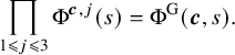
Thus, in order to use (3.13) (which concerns
$\Phi ^{\boldsymbol {c},1}$
 ) to bound
$\Phi ^{\text {G}}(\boldsymbol {c},s)$
) to bound
$\Phi ^{\text {G}}(\boldsymbol {c},s)$
 , we will first need to control the factors
$\Phi ^{\boldsymbol {c},2}$
, we will first need to control the factors
$\Phi ^{\boldsymbol {c},2}$
 and
$\Phi ^{\boldsymbol {c},3}$
and
$\Phi ^{\boldsymbol {c},3}$
 on average over
$\boldsymbol {c}$
on average over
$\boldsymbol {c}$
 .
.
Proposition 4.2. Let
$Z,R\in \mathbb {Z}$
 and
$A, \varepsilon \in \mathbb {R}_{>0}$
and
$A, \varepsilon \in \mathbb {R}_{>0}$
 . Then

Proof. If
$\widehat R\leqslant 1$
 then (4.2) is trivial, so suppose
$\widehat R>1$
then (4.2) is trivial, so suppose
$\widehat R>1$
 . By Hölder’s inequality, we may assume A is an even integer. Let
$\Sigma (Z,R)$
. By Hölder’s inequality, we may assume A is an even integer. Let
$\Sigma (Z,R)$
 denote the left-hand side of (4.2) and put

We claim that for
$Z\geqslant AR$
 we have

To prove this, we write
$\lvert \sum _{\lvert r \rvert =\widehat R} a_{\boldsymbol {c},2}(r) \rvert ^A = \sum _{\lvert r_1 \rvert =\dots =\lvert r_A \rvert =\widehat R} a_{\boldsymbol {c},2}(r_1)\cdots a_{\boldsymbol {c},2}(r_A)$
 , on noting that
$a_{\boldsymbol {c},2}(r)\in \mathbb {R}$
, on noting that
$a_{\boldsymbol {c},2}(r)\in \mathbb {R}$
 . If
$r_1\cdots r_A = M$
. If
$r_1\cdots r_A = M$
 , then (by smooth proper base change) the function
$\boldsymbol {c}\mapsto a_{\boldsymbol {c},2}(r_1)\cdots a_{\boldsymbol {c},2}(r_A)$
, then (by smooth proper base change) the function
$\boldsymbol {c}\mapsto a_{\boldsymbol {c},2}(r_1)\cdots a_{\boldsymbol {c},2}(r_A)$
 is constant on each fibre of the map

Each fibre has cardinality
$(\widehat Z/\lvert M \rvert )^6$
 , since
$1<\lvert M \rvert \leqslant \widehat R^A\leqslant \widehat Z$
, since
$1<\lvert M \rvert \leqslant \widehat R^A\leqslant \widehat Z$
 . The claim follows.
By GRH (Proposition 3.1(5)), we have
$\Sigma (Z,R) \ll _{A,\varepsilon } \widehat Z^{6+\varepsilon } \widehat R^{A/4+\varepsilon }$
 for all
$\widehat Z>0$
for all
$\widehat Z>0$
 . (The exponent is
$A/4$
. (The exponent is
$A/4$
 rather than
$A/2$
rather than
$A/2$
 , because the Euler product of
$\Phi ^{\boldsymbol {c},2}(s)$
, because the Euler product of
$\Phi ^{\boldsymbol {c},2}(s)$
 , as given in Definition 4.1, is supported on square moduli due to the appearance of
$2s$
, as given in Definition 4.1, is supported on square moduli due to the appearance of
$2s$
 .) Thus
$ \widetilde {\Sigma }(Z,R) \ll _{A,\varepsilon } \widehat R^{A/4+\varepsilon } $
.) Thus
$ \widetilde {\Sigma }(Z,R) \ll _{A,\varepsilon } \widehat R^{A/4+\varepsilon } $
 for
$Z\leqslant AR$
for
$Z\leqslant AR$
 , and so for all Z, by (4.3).
Proposition 4.3. For
$\boldsymbol {c}\in \mathcal {S}_1$
 , primes
$\varpi \in \mathcal {O}^+$
, primes
$\varpi \in \mathcal {O}^+$
 , and integers
$l\geqslant 1$
, and integers
$l\geqslant 1$
 , we have

Proof. If
$\varpi \mid F^\ast (\boldsymbol {c})$
 , then
$\Phi ^{\text {G}}_\varpi (\boldsymbol {c},s) = 1$
, then
$\Phi ^{\text {G}}_\varpi (\boldsymbol {c},s) = 1$
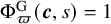 . If
$\varpi \nmid F^\ast (\boldsymbol {c})$
. If
$\varpi \nmid F^\ast (\boldsymbol {c})$
 , then (2.17) implies

because
$S^\natural _\varpi (\boldsymbol {c}) = E^\natural _{\boldsymbol {c}}(\mathcal {O}/\varpi \mathcal {O})-\lvert \varpi \rvert ^{-1/2}E^\natural _F(\mathcal {O}/\varpi \mathcal {O})$
 by (2.16) and

by the Grothendieck–Lefschetz trace formula. In either case,
$a_{\boldsymbol {c},3}(\varpi ^l)\ll _\varepsilon \lvert \varpi \rvert ^{l\varepsilon }$
 follows from the Ramanujan bound
$\lvert \alpha \rvert \leqslant 1$
follows from the Ramanujan bound
$\lvert \alpha \rvert \leqslant 1$
 in Proposition 3.1(3).
Now suppose
$\varpi \nmid F^\ast (\boldsymbol {c})$
 . Multiplying
$\Phi ^{\text {G}}_\varpi (\boldsymbol {c},s)$
. Multiplying
$\Phi ^{\text {G}}_\varpi (\boldsymbol {c},s)$
 by
by

and discarding all terms of the form
$O(\lvert \varpi \rvert ^{-s} \times \lvert \varpi \rvert ^{-2s})$
 or
$O(\lvert \varpi \rvert ^{-s} \times \lvert \varpi \rvert ^{-1/2-s})$
or
$O(\lvert \varpi \rvert ^{-s} \times \lvert \varpi \rvert ^{-1/2-s})$
 , we get

since
$\lambda _{\boldsymbol {c}}(\varpi )^2 = \lambda _{\boldsymbol {c}}(\varpi ^2) + \lambda _{\boldsymbol {c},\bigwedge ^2}(\varpi )$
 . This completes the proof of the proposition.
Corollary 4.4. Let
$Z,R\in \mathbb {Z}$
 and
$A, \varepsilon \in \mathbb {R}_{>0}$
and
$A, \varepsilon \in \mathbb {R}_{>0}$
 . Then

Proof. By multiplicativity (of
$\lvert a_{\boldsymbol {c},3} \rvert $
 ) and positivity, we have

But by Proposition 4.3, we have
$a_{\boldsymbol {c},3}(d)\ll _\varepsilon \lvert d \rvert ^\varepsilon $
 and
and

So by (4.4), the quantity to be estimated is

Now the claimed bound follows from Lemma 2.3.
Conjecture 4.5. Let
$\varepsilon \in (0,1]$
 . Let
$Z,R\in \mathbb {Z}$
. Let
$Z,R\in \mathbb {Z}$
 with
$R\leqslant 3Z$
with
$R\leqslant 3Z$
 . Then

Proof assuming Conjecture 3.8
Let
$\boldsymbol {c}\in \mathcal {S}_1$
 and
$R_1,R_2,R_3\in \mathbb {Z}_{\geqslant 0}$
and
$R_1,R_2,R_3\in \mathbb {Z}_{\geqslant 0}$
 . Writing

for brevity, we have

since
$\Phi ^{\text {G}} = \Phi ^{\boldsymbol {c},1} \Phi ^{\boldsymbol {c},2} \Phi ^{\boldsymbol {c},3}$
 . Let
$\beta := 2-\varepsilon $
. Let
$\beta := 2-\varepsilon $
 . Let
. Let

for some
$\eta>0$
 to be chosen. Let
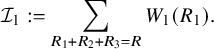
Using Hölder’s inequality in the form
$1 = \frac {\beta -1}{\beta } + \frac {1}{\beta }$
 over the set
$\{R_1+R_2+R_3=R\}$
over the set
$\{R_1+R_2+R_3=R\}$
 (and then exponentiating by
$\beta $
(and then exponentiating by
$\beta $
 ), we obtain

since
$\beta \geqslant 1$
 and
$W_1^{\beta -1} W_2 = 1$
and
$W_1^{\beta -1} W_2 = 1$
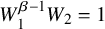 . Here
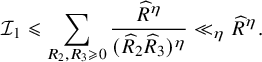
Upon summing (4.6) over
$\lvert \boldsymbol {c} \rvert \leqslant \widehat Z$
 , we thus find that the left-hand side of (4.5) is

Let
$(\gamma _1, \gamma _2, \gamma _3) := (2, 4\beta /\varepsilon , 4\beta /\varepsilon )$
 . Then
$\sum _{1\leqslant j\leqslant 3} \beta /\gamma _j = 1$
. Then
$\sum _{1\leqslant j\leqslant 3} \beta /\gamma _j = 1$
 , so by Hölder over
$\boldsymbol {c}$
, so by Hölder over
$\boldsymbol {c}$
 , we obtain

where
$\mathscr {M}_j = \sum _{\boldsymbol {c}\in \mathcal {S}_1:\, \lvert \boldsymbol {c} \rvert \leqslant \widehat Z} \lvert \Sigma ^{\boldsymbol {c},j}(R_j) \rvert ^{\gamma _j}$
 . By Conjecture 3.8 with
$R_1$
. By Conjecture 3.8 with
$R_1$
 in place of R, we have
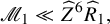
since
$R_1\leqslant R\leqslant 3Z$
 by assumption. Also, by (4.2) and Corollary 4.4, we have

Therefore, if
$R_1+R_2+R_3=R$
 , then the right-hand side of (4.8) is

Plugging (4.8) into (4.7) now bounds the left-hand side of (4.5) by

Let
$\eta = \min (9/40, 2/15)$
 . Then
$R_1+R_2+R_3=R \Rightarrow (\widehat R/\widehat R_1)^\eta \leqslant \widehat R_2^{9/40} \widehat R_3^{2/15}$
. Then
$R_1+R_2+R_3=R \Rightarrow (\widehat R/\widehat R_1)^\eta \leqslant \widehat R_2^{9/40} \widehat R_3^{2/15}$
 . Since
$\beta -1\geqslant 0$
. Since
$\beta -1\geqslant 0$
 , it follows that the quantity (4.9) is

This implies the desired inequality (4.5).
5 Integral estimates
Let
$\gamma \in K_\infty $
 ,
$\boldsymbol {w}\in K_\infty ^n$
,
$\boldsymbol {w}\in K_\infty ^n$
 and
$G\in K_\infty [x_1,\dots , x_n]$
and
$G\in K_\infty [x_1,\dots , x_n]$
 . For a fixed smooth weight function
$w\colon K_\infty ^n\to \mathbb {R}$
. For a fixed smooth weight function
$w\colon K_\infty ^n\to \mathbb {R}$
 with compact support, we are interested in integrals of the form

together with their averages

for
$\Gamma \in \mathbb {Z}$
 . (In fact, the dependence of the latter integral on
$\Gamma $
. (In fact, the dependence of the latter integral on
$\Gamma $
 is mild, as we will soon see.) With this notation we have
$I_r(\theta ,\boldsymbol {c})=J_{F,w}(\theta P^3,P\boldsymbol {c}/r)$
is mild, as we will soon see.) With this notation we have
$I_r(\theta ,\boldsymbol {c})=J_{F,w}(\theta P^3,P\boldsymbol {c}/r)$
 in (2.7) and
$I_r(\boldsymbol {c})=\lvert P \rvert ^{-3}J_{F,w}^{\Gamma }(P\boldsymbol {c}/r)$
in (2.7) and
$I_r(\boldsymbol {c})=\lvert P \rvert ^{-3}J_{F,w}^{\Gamma }(P\boldsymbol {c}/r)$
 in (2.8), where
$\Gamma =-\deg (r)-Q+3\deg (P)$
in (2.8), where
$\Gamma =-\deg (r)-Q+3\deg (P)$
 .
.
When w is the indicator function of
$\mathbb {T}^n$
 , we shall write
$J_G(\gamma ,\boldsymbol {w})$
, we shall write
$J_G(\gamma ,\boldsymbol {w})$
 and
$J^\Gamma _G(\boldsymbol {w})$
and
$J^\Gamma _G(\boldsymbol {w})$
 for the sake of brevity. Moreover, we let
$H_G$
for the sake of brevity. Moreover, we let
$H_G$
 be the maximum of the absolute values of the coefficients of G and refer to it as the height of G.
This level of generality, where G is allowed to vary, will be useful when changing variables to analyse
$J^\Gamma _{F,w}(\boldsymbol {w})$
 . Let us recall Lemmas 2.4 and 2.7 of [Reference Browning and Vishe12].
Lemma 5.1. Let
$G\in K_\infty [x_1,\dots , x_n]$
 and
$\boldsymbol {w}\in K_\infty ^n$
and
$\boldsymbol {w}\in K_\infty ^n$
 . Suppose
$|\boldsymbol {w}|\geqslant 1$
. Suppose
$|\boldsymbol {w}|\geqslant 1$
 and
$|\boldsymbol {w}|>H_G$
and
$|\boldsymbol {w}|>H_G$
 . Then

Lemma 5.2. Let

Then we have

We now fix a nonsingular cubic form
$F\in \mathcal {O}[x_1,\dots , x_n]$
 , which we will eventually take to be our initial cubic form
$x_1^3+\cdots + x_6^3$
, which we will eventually take to be our initial cubic form
$x_1^3+\cdots + x_6^3$
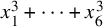 , but is allowed to be arbitrary in this section. Before we start our investigation, we impose the following conditions on the weight function w.
Hypothesis 5.3. Let
$H(\boldsymbol {x})=(\frac {\partial ^{2}F(\boldsymbol {x})}{\partial x_i\partial x_j})$
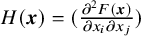 be the Hessian associated to F.
-
(i) If $\boldsymbol {x}\in \operatorname {\mathrm {supp}}(w)$
, then
$\det H(\boldsymbol {x})\neq 0$
. -
(ii) There exist $\boldsymbol {x_0}\in K_\infty ^n$
with
$\lvert \boldsymbol {x}_0 \rvert \leqslant 1$
, and an integer
$L\geqslant 0$
, such that $$\begin{align*}w(\boldsymbol{x})=\begin{cases} 1 &\text{if }|\boldsymbol{x}-\boldsymbol{x}_0|<\widehat{L}^{-1},\\ 0&\text{else.} \end{cases} \end{align*}$$




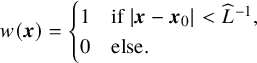
If
$\operatorname {\mathrm {char}}(\mathbb {F}_q)\in \{2,3\}$
 , then
$\det H(\boldsymbol {x})$
, then
$\det H(\boldsymbol {x})$
 vanishes identically and so (i) is impossible in this case. Therefore, all of our results in this section have the implicit assumption that
$\operatorname {\mathrm {char}}(\mathbb {F}_q)>3$
vanishes identically and so (i) is impossible in this case. Therefore, all of our results in this section have the implicit assumption that
$\operatorname {\mathrm {char}}(\mathbb {F}_q)>3$
 . Moreover, condition (ii) is nonrestrictive, since any compactly supported smooth function
$w'\colon K_\infty ^n\to \mathbb {R}$
. Moreover, condition (ii) is nonrestrictive, since any compactly supported smooth function
$w'\colon K_\infty ^n\to \mathbb {R}$
 can be written as
$w'= s_1 w_1+\cdots +s_mw_m$
can be written as
$w'= s_1 w_1+\cdots +s_mw_m$
 , where
$s_i\in \mathbb {R}$
, where
$s_i\in \mathbb {R}$
 and
$w_i$
and
$w_i$
 are indicator functions of some compact ball in
$K_\infty ^n$
are indicator functions of some compact ball in
$K_\infty ^n$
 . Part (ii) of Hypothesis 5.3 implies the crucial symmetry property

In other words, w is invariant under scaling by
$1+t^{-L}\mathbb {T}$
 . Throughout this section, all implied constants are allowed to depend on the choice of w and in particular implicitly also on the parameter L and the vector
$\boldsymbol {x}_0$
. Throughout this section, all implied constants are allowed to depend on the choice of w and in particular implicitly also on the parameter L and the vector
$\boldsymbol {x}_0$
 in the definition of w.
For the purposes of Theorem 1.1, we will be focusing on diagonal cubic forms. In this setting we shall work with the following explicit weight function.
Definition 5.4. Let
$F(\boldsymbol {x})=a_1x_1^3+\cdots +a_nx_n^3$
 , for
$a_1,\dots ,a_n\in \mathbb {F}_q^\times $
, for
$a_1,\dots ,a_n\in \mathbb {F}_q^\times $
 and let
$\boldsymbol {x}_0\in (\mathbb {F}_q^\times )^n$
and let
$\boldsymbol {x}_0\in (\mathbb {F}_q^\times )^n$
 be such that
$F(\boldsymbol {x}_0)=0$
be such that
$F(\boldsymbol {x}_0)=0$
 . Then we define a weight function
$w=w_{\boldsymbol {x}_0}$
. Then we define a weight function
$w=w_{\boldsymbol {x}_0}$
 by the formula
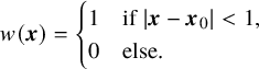
We check that such weight functions satisfy Hypothesis 5.3 when F is a diagonal cubic form with coefficients in
$\mathbb {F}_q^\times $
 and
$\operatorname {\mathrm {char}}(\mathbb {F}_q)>3$
and
$\operatorname {\mathrm {char}}(\mathbb {F}_q)>3$
 . Condition (i) can then be rephrased as
$x_1\cdots x_n\neq 0$
. Condition (i) can then be rephrased as
$x_1\cdots x_n\neq 0$
 for all
$\boldsymbol {x}\in \operatorname {\mathrm {supp}}(w)$
for all
$\boldsymbol {x}\in \operatorname {\mathrm {supp}}(w)$
 , which is obvious. Condition (ii) clearly holds with
$L=0$
, which is obvious. Condition (ii) clearly holds with
$L=0$
 .
.
Returning to the setting of general weight functions w satisfying Hypothesis 5.3, we begin with the following estimate.
Lemma 5.5. For
$\Gamma \in \mathbb {Z}$
 and
$\boldsymbol {w}\in K_\infty ^n$
and
$\boldsymbol {w}\in K_\infty ^n$
 , we have

Moreover, if
$|\boldsymbol {w}|\gg 1$
 , then
$J_{F,w}(\gamma , \boldsymbol {w})=0$
, then
$J_{F,w}(\gamma , \boldsymbol {w})=0$
 unless
$|\gamma |\asymp |\boldsymbol {w}|$
unless
$|\gamma |\asymp |\boldsymbol {w}|$
 .
.
Proof. In this proof all implied constants are allowed to depend on F. Upon making the change of variables
$\boldsymbol {y}=t^L(\boldsymbol {x}-\boldsymbol {x}_0)$
 , it follows that

where
$G(\boldsymbol {y})=F(t^{-L}\boldsymbol {y}+\boldsymbol {x}_0)$
 . It is clear that
$H_G\ll H_F\ll 1$
. It is clear that
$H_G\ll H_F\ll 1$
 . At this point we can use Lemma 5.1 to conclude that
$J_{F,w}(\gamma , \boldsymbol {w})=0$
. At this point we can use Lemma 5.1 to conclude that
$J_{F,w}(\gamma , \boldsymbol {w})=0$
 unless
$|\boldsymbol {w}|\ll \text {max}\{1, |\gamma |\}$
unless
$|\boldsymbol {w}|\ll \text {max}\{1, |\gamma |\}$
 . Furthermore, by Lemma 5.2

since
$\nabla G(\boldsymbol {y}) = t^{-L}\nabla F(\boldsymbol {x})$
 . Let us denote the set whose measure we want to estimate by
$\Omega $
. Let us denote the set whose measure we want to estimate by
$\Omega $
 . Since
$\boldsymbol {0}\not \in \operatorname {\mathrm {supp}}(w)$
. Since
$\boldsymbol {0}\not \in \operatorname {\mathrm {supp}}(w)$
 , we must have
$|\nabla F(\boldsymbol {x})|\asymp 1$
, we must have
$|\nabla F(\boldsymbol {x})|\asymp 1$
 for all
$\boldsymbol {x}\in \operatorname {\mathrm {supp}}(w)$
for all
$\boldsymbol {x}\in \operatorname {\mathrm {supp}}(w)$
 . If
$|\boldsymbol {w}|\ll 1$
. If
$|\boldsymbol {w}|\ll 1$
 , then
$\Omega $
, then
$\Omega $
 is empty unless
$|\gamma |\ll 1$
is empty unless
$|\gamma |\ll 1$
 , so that we can use the trivial estimate
$|J_{F,w}(\gamma ,\boldsymbol {w})|\leqslant 1$
, so that we can use the trivial estimate
$|J_{F,w}(\gamma ,\boldsymbol {w})|\leqslant 1$
 to conclude that
$J^\Gamma _{F,w}(\boldsymbol {w})\ll 1$
to conclude that
$J^\Gamma _{F,w}(\boldsymbol {w})\ll 1$
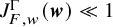 if
$|\boldsymbol {w}|\ll 1 $
if
$|\boldsymbol {w}|\ll 1 $
 . In particular, we may assume
$|\boldsymbol {w}|\gg 1$
. In particular, we may assume
$|\boldsymbol {w}|\gg 1$
 for the rest of the proof. In this case the contribution from
$|\gamma |\ll 1$
for the rest of the proof. In this case the contribution from
$|\gamma |\ll 1$
 vanishes, since then
$\Omega $
vanishes, since then
$\Omega $
 is empty, while for
$|\gamma |\gg 1$
is empty, while for
$|\gamma |\gg 1$
 the defining inequality for
$\Omega $
the defining inequality for
$\Omega $
 becomes

This can only hold if
$|\gamma |\asymp |\boldsymbol {w}|$
 . From this we deduce the statement that
$J_{F,w}(\gamma ,\boldsymbol {w})=0$
. From this we deduce the statement that
$J_{F,w}(\gamma ,\boldsymbol {w})=0$
 unless
$|\gamma |\asymp |\boldsymbol {w}|$
unless
$|\gamma |\asymp |\boldsymbol {w}|$
 .
.
It remains to give an upper bound. This will be similar to [Reference Browning and Vishe12, proof of Lemma 7.3]. Let us now assume that
$\boldsymbol {x}, \boldsymbol {x}+\boldsymbol {x}'$
 are both in
$\Omega $
are both in
$\Omega $
 . Note that
$\nabla F(\boldsymbol {x}+\boldsymbol {x}')-\nabla F (\boldsymbol {x})= H(\boldsymbol {x}+\boldsymbol {x}'/2)\boldsymbol {x}'$
. Note that
$\nabla F(\boldsymbol {x}+\boldsymbol {x}')-\nabla F (\boldsymbol {x})= H(\boldsymbol {x}+\boldsymbol {x}'/2)\boldsymbol {x}'$
 , so that we must then have

As
$\det H(\boldsymbol {y})\neq 0$
 for all
$\boldsymbol {y}\in \operatorname {\mathrm {supp}}(w)$
for all
$\boldsymbol {y}\in \operatorname {\mathrm {supp}}(w)$
 , compactness of
$\operatorname {\mathrm {supp}}(w)$
, compactness of
$\operatorname {\mathrm {supp}}(w)$
 implies that we have
$|\det H(\boldsymbol {y})|\gg 1$
implies that we have
$|\det H(\boldsymbol {y})|\gg 1$
 for all
$\boldsymbol {y}\in \operatorname {\mathrm {supp}}(w)$
for all
$\boldsymbol {y}\in \operatorname {\mathrm {supp}}(w)$
 . In addition, a straightforward computation shows that
$\boldsymbol {x}+\boldsymbol {x}'/2\in \operatorname {\mathrm {supp}}(w)$
. In addition, a straightforward computation shows that
$\boldsymbol {x}+\boldsymbol {x}'/2\in \operatorname {\mathrm {supp}}(w)$
 , so that we can multiply (5.2) from the left by the inverse of
$H(\boldsymbol {x}+\boldsymbol {x}'/2)$
, so that we can multiply (5.2) from the left by the inverse of
$H(\boldsymbol {x}+\boldsymbol {x}'/2)$
 , whose entries have absolute value
$O(1)$
, whose entries have absolute value
$O(1)$
 , to conclude that
$|\boldsymbol {x}'|\ll |\gamma |^{-1/2}\ll |\boldsymbol {w}|^{-1/2}$
, to conclude that
$|\boldsymbol {x}'|\ll |\gamma |^{-1/2}\ll |\boldsymbol {w}|^{-1/2}$
 . Finally, from this we obtain

when
$|\boldsymbol {w}|\gg 1$
 , as desired.
The following symmetry property of
$J^\Gamma _{F,w}(\boldsymbol {w})$
 generalises [Reference Glas and Hochfilzer26, Lemma 3.6].
Lemma 5.6. Suppose
$\lambda _1,\lambda _2 \in K_\infty ^\times $
 are such that
$\lambda _1/\lambda _2\in 1+t^{-L}\mathbb {T}$
are such that
$\lambda _1/\lambda _2\in 1+t^{-L}\mathbb {T}$
 . Then

Proof. Let us write
$\lambda =\lambda _1$
 and show that for
$\boldsymbol {w}$
and show that for
$\boldsymbol {w}$
 fixed, the value of
$J^\Gamma _{F,w}(\lambda \boldsymbol {w})$
fixed, the value of
$J^\Gamma _{F,w}(\lambda \boldsymbol {w})$
 only depends on the image of
$\lambda $
only depends on the image of
$\lambda $
 in the quotient group
$K_\infty ^\times / (1+t^{-L}\mathbb {T})$
in the quotient group
$K_\infty ^\times / (1+t^{-L}\mathbb {T})$
 . We have

where we applied the change of variables
$\boldsymbol {y}=\lambda \boldsymbol {x}$
 . It follows from (2.3) that

This formula clearly only depends on
$|\lambda |$
 . Moreover,
$w(\lambda ^{-1}\boldsymbol {y})$
. Moreover,
$w(\lambda ^{-1}\boldsymbol {y})$
 depends only on
$\lambda \bmod {1+t^{-L}\mathbb {T}}$
depends only on
$\lambda \bmod {1+t^{-L}\mathbb {T}}$
 by (5.1). Since we assume
$L\geqslant 0$
by (5.1). Since we assume
$L\geqslant 0$
 , any two elements of
$K_\infty ^\times $
, any two elements of
$K_\infty ^\times $
 whose image in
$K_\infty ^\times / (1+t^{-L}\mathbb {T})$
whose image in
$K_\infty ^\times / (1+t^{-L}\mathbb {T})$
 coincides must have the same absolute value, from which we deduce that
$J^\Gamma _{F,w}(\lambda \boldsymbol {w})$
coincides must have the same absolute value, from which we deduce that
$J^\Gamma _{F,w}(\lambda \boldsymbol {w})$
 only depends on
$\lambda \bmod {1+t^{-L}\mathbb {T}}$
only depends on
$\lambda \bmod {1+t^{-L}\mathbb {T}}$
 .
.
The above establishes most of the analogue over K of [Reference Wang57, Proposition 8.1]. It still remains to show that
$J^\Gamma _{F,w}(\boldsymbol {w})$
 vanishes unless
$|F^*(\boldsymbol {w})|$
vanishes unless
$|F^*(\boldsymbol {w})|$
 is small. Working over function fields significantly simplifies the execution of the key ideas, because fewer dyadic ranges intervene. We start with an auxiliary lemma.
Lemma 5.7. Let R be a compact set such that
$ R\subset \{\boldsymbol {x}\in K_\infty ^n\colon \det H(\boldsymbol {x})\neq 0\}$
 . Then there exists a constant
$C=C(R)>0$
. Then there exists a constant
$C=C(R)>0$
 such that if
$\boldsymbol {w}\in K_\infty ^n$
such that if
$\boldsymbol {w}\in K_\infty ^n$
 and
$\boldsymbol {x}\in R$
and
$\boldsymbol {x}\in R$
 satisfy

it follows that there exists
$\boldsymbol {s} \in K_\infty ^n$
 with
$\nabla F(\boldsymbol {s})= \boldsymbol {w}$
with
$\nabla F(\boldsymbol {s})= \boldsymbol {w}$
 and
and

Proof. Let
$\boldsymbol {x}\in R$
 . Since
$\det H(\boldsymbol {x}) \neq 0$
. Since
$\det H(\boldsymbol {x}) \neq 0$
 , it follows from the inverse function theorem for local fields [Reference Serre48, Part II, § III.9, Theorem 2] that there exist open neighbourhoods
$U, U'\subset K_\infty ^n$
, it follows from the inverse function theorem for local fields [Reference Serre48, Part II, § III.9, Theorem 2] that there exist open neighbourhoods
$U, U'\subset K_\infty ^n$
 , with
$\det H(\boldsymbol {y})\neq 0$
, with
$\det H(\boldsymbol {y})\neq 0$
 for any
$\boldsymbol {y}$
for any
$\boldsymbol {y}$
 in the closure of U, such that
$\boldsymbol {x}\in U$
in the closure of U, such that
$\boldsymbol {x}\in U$
 ,
$\nabla F(\boldsymbol {x})\in U'$
,
$\nabla F(\boldsymbol {x})\in U'$
 and
$\nabla F\colon U \to U'$
and
$\nabla F\colon U \to U'$
 is an isomorphism. In addition, after shrinking
$U'$
is an isomorphism. In addition, after shrinking
$U'$
 if necessary, we may assume that it is an open ball of radius
$\widehat C_0^{-1}$
if necessary, we may assume that it is an open ball of radius
$\widehat C_0^{-1}$
 around
$\nabla F(\boldsymbol {x})$
around
$\nabla F(\boldsymbol {x})$
 , for some real
$C_0=C_0(\boldsymbol {x})\geqslant 0$
, for some real
$C_0=C_0(\boldsymbol {x})\geqslant 0$
 . It follows that if
$\boldsymbol {w} \in U'$
. It follows that if
$\boldsymbol {w} \in U'$
 , there exists
$\boldsymbol {s}\in U$
, there exists
$\boldsymbol {s}\in U$
 such that
$\nabla F(\boldsymbol {s})= \boldsymbol {w}$
such that
$\nabla F(\boldsymbol {s})= \boldsymbol {w}$
 . Therefore, we have

As
$\boldsymbol {x}\in R$
 , we have
$\det H(\boldsymbol {x})\neq 0$
, we have
$\det H(\boldsymbol {x})\neq 0$
 , and hence

Moreover, as R is compact, the entries of
$H(\boldsymbol {x})^{-1}$
 are
$O_R(1)$
are
$O_R(1)$
 . It follows that there exist constants
$C_1, C_2\geqslant 0$
. It follows that there exist constants
$C_1, C_2\geqslant 0$
 depending only on R and F such that

Upon shrinking U if necessary, we may assume that
$|\boldsymbol {s}-\boldsymbol {x}|< (2\widehat {C}_2)^{-1}$
 , so that we obtain

Since R is compact, we can cover it with finitely many open sets U and then take C to be the maximum of the constants that arise in this process.
Lemma 5.8. Assume
$L=0$
 in condition (ii) on the weight function w. Let
$\Gamma \in \mathbb {Z}$
in condition (ii) on the weight function w. Let
$\Gamma \in \mathbb {Z}$
 and
$\boldsymbol {w}\in K_\infty ^n$
and
$\boldsymbol {w}\in K_\infty ^n$
 . Then
$J^\Gamma _{F,w}(\boldsymbol {w})=0$
. Then
$J^\Gamma _{F,w}(\boldsymbol {w})=0$
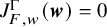 unless
$|F^*({\boldsymbol {w}})|\ll 1+ |\boldsymbol {w}|^{\deg F^*-1}$
unless
$|F^*({\boldsymbol {w}})|\ll 1+ |\boldsymbol {w}|^{\deg F^*-1}$
 .
.
Proof. Note that if
$|\boldsymbol {w}|\ll 1$
 , then
$|F^*({\boldsymbol {w}})|\ll 1+|\boldsymbol {w}|^{\deg F^*-1}$
, then
$|F^*({\boldsymbol {w}})|\ll 1+|\boldsymbol {w}|^{\deg F^*-1}$
 holds trivially, so that we may assume
$|\boldsymbol {w}|\gg 1$
holds trivially, so that we may assume
$|\boldsymbol {w}|\gg 1$
 from now on. Similarly we can assume
$1\ll |\boldsymbol {w}|\ll \widehat {\Gamma }$
from now on. Similarly we can assume
$1\ll |\boldsymbol {w}|\ll \widehat {\Gamma }$
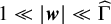 , since otherwise
$J^\Gamma _{F,w}(\boldsymbol {w})=0$
, since otherwise
$J^\Gamma _{F,w}(\boldsymbol {w})=0$
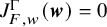 by Lemma 5.5. Using Lemma 5.5 again, it follows that

Let
$Z\in \mathbb {Z}_{>0}$
 be such that
$\widehat {Z}\asymp |\boldsymbol {w}|$
be such that
$\widehat {Z}\asymp |\boldsymbol {w}|$
 . We will now consider the contribution to
$J^\Gamma _{F,w}(\boldsymbol {w})$
. We will now consider the contribution to
$J^\Gamma _{F,w}(\boldsymbol {w})$
 from those
$\gamma $
from those
$\gamma $
 with
$|\gamma |=\widehat {Z}$
with
$|\gamma |=\widehat {Z}$
 . To do so, write
$\gamma = a t^Z(1+\gamma ')$
. To do so, write
$\gamma = a t^Z(1+\gamma ')$
 , where
$a\in \mathbb {F}_q^\times $
, where
$a\in \mathbb {F}_q^\times $
 and
$\gamma '\in \mathbb {T}$
and
$\gamma '\in \mathbb {T}$
 . Let
$\boldsymbol {y} := \boldsymbol {x}-\boldsymbol {x}_0$
. Let
$\boldsymbol {y} := \boldsymbol {x}-\boldsymbol {x}_0$
 and
$G(\boldsymbol {y}) := F(\boldsymbol {y}+\boldsymbol {x}_0)$
and
$G(\boldsymbol {y}) := F(\boldsymbol {y}+\boldsymbol {x}_0)$
 , as in the proof of Lemma 5.5. Then let

Note that since
$(1+\gamma ')^{-1/2} - 1 \in \mathbb {T}$
 and
$L=0$
and
$L=0$
 , property (5.1) of the weight function w implies
$w(\boldsymbol {x})=w(\boldsymbol {x}')$
, property (5.1) of the weight function w implies
$w(\boldsymbol {x})=w(\boldsymbol {x}')$
 . In particular, after the change of variables
$\boldsymbol {x}\mapsto (1+\gamma ')^{-1/2}\boldsymbol {x}$
. In particular, after the change of variables
$\boldsymbol {x}\mapsto (1+\gamma ')^{-1/2}\boldsymbol {x}$
 by condition (ii) on w, we get

by Lemma 5.2, where

and we used that
$\gamma F(\boldsymbol {x}')=at^Z (1+\gamma ')^{-1/2}F(\boldsymbol {y}+\boldsymbol {x}_0)$
 since F is homogeneous of degree
$3$
since F is homogeneous of degree
$3$
 . In summary, we have proven the identity

and applied stationary phase to the latter integral to get an integral over
$\boldsymbol {y}\in \Omega $
 .
.
Upon expressing the integral over
$\boldsymbol {y}\in \Omega $
 in terms of
$\boldsymbol {x} = \boldsymbol {y}+\boldsymbol {x}_0$
in terms of
$\boldsymbol {x} = \boldsymbol {y}+\boldsymbol {x}_0$
 , we find that

where
$\Phi (\boldsymbol {x}) := at^ZF(\boldsymbol {x})+\boldsymbol {w}\cdot \boldsymbol {x}$
 and
and

The crucial observation here is that
$\Omega '$
 is independent of
$\gamma '$
is independent of
$\gamma '$
 . In particular, when considering the total contribution to
$J^\Gamma _{F,w}(\boldsymbol {w})$
. In particular, when considering the total contribution to
$J^\Gamma _{F,w}(\boldsymbol {w})$
 from the set
$\{\gamma = at^Z(1+\gamma '): \gamma '\in \mathbb {T}\}$
from the set
$\{\gamma = at^Z(1+\gamma '): \gamma '\in \mathbb {T}\}$
 , we may exchange the order of integration and see that it is given by

Here
$\Omega '$
 ,
$\Phi $
,
$\Phi $
 depend on Z and a, but all estimates below will be uniform over Z and a. Let us now take the Taylor expansion
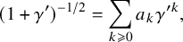
where
$a_k=\binom {-1/2}{k}\in \mathbb {F}_q$
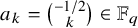 . This is well defined, because
$|\gamma '|<1$
. This is well defined, because
$|\gamma '|<1$
 and
$\operatorname {\mathrm {char}}(\mathbb {F}_q)\neq 2$
and
$\operatorname {\mathrm {char}}(\mathbb {F}_q)\neq 2$
 . Since
$|\gamma '|<1$
. Since
$|\gamma '|<1$
 , the value of
$\psi ((1+\gamma ')^{-1/2}\Phi (\boldsymbol {x}))$
, the value of
$\psi ((1+\gamma ')^{-1/2}\Phi (\boldsymbol {x}))$
 only depends on
$f(\gamma ')=\sum _{k=0}^{k_0}a_k \gamma ^{\prime k}$
only depends on
$f(\gamma ')=\sum _{k=0}^{k_0}a_k \gamma ^{\prime k}$
 if we choose
$k_0$
if we choose
$k_0$
 sufficiently large. We may now apply Lemma 5.2 again with
$n=1$
sufficiently large. We may now apply Lemma 5.2 again with
$n=1$
 to infer that the inner integral is given by
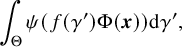
where

It is easy to see that
$|f'(\gamma ')|=1$
 , so that
$\Theta $
, so that
$\Theta $
 is nonempty only if
$|\Phi (\boldsymbol {x})|\leqslant 1$
is nonempty only if
$|\Phi (\boldsymbol {x})|\leqslant 1$
 , which we shall assume for the rest of the proof.
Since
$\boldsymbol {x}\in \Omega '$
 , we have
$\boldsymbol {x}\in \operatorname {\mathrm {supp}}(w)$
, we have
$\boldsymbol {x}\in \operatorname {\mathrm {supp}}(w)$
 and
$|a\nabla F(\boldsymbol {x})+t^{-Z}\boldsymbol {w}|\ll \widehat {Z}^{-1/2}\ll |\boldsymbol {w}|^{-1/2}$
and
$|a\nabla F(\boldsymbol {x})+t^{-Z}\boldsymbol {w}|\ll \widehat {Z}^{-1/2}\ll |\boldsymbol {w}|^{-1/2}$
 . Since we assume
$|\boldsymbol {w}|\gg 1$
. Since we assume
$|\boldsymbol {w}|\gg 1$
 for a sufficiently large implied constant, we may invoke Lemma 5.7 to deduce the existence of
$\boldsymbol {s}\in K_\infty ^n$
for a sufficiently large implied constant, we may invoke Lemma 5.7 to deduce the existence of
$\boldsymbol {s}\in K_\infty ^n$
 such that
$|\boldsymbol {s}-\boldsymbol {x}|\ll |a \nabla F(\boldsymbol {x})+t^{-Z}\boldsymbol {w}|\ll |\boldsymbol {w}|^{-1/2}$
such that
$|\boldsymbol {s}-\boldsymbol {x}|\ll |a \nabla F(\boldsymbol {x})+t^{-Z}\boldsymbol {w}|\ll |\boldsymbol {w}|^{-1/2}$
 and
$\nabla F(\boldsymbol {s})=-a^{-1}t^{-Z}\boldsymbol {w}$
and
$\nabla F(\boldsymbol {s})=-a^{-1}t^{-Z}\boldsymbol {w}$
 . Using Taylor expansion at
$\boldsymbol {s}$
. Using Taylor expansion at
$\boldsymbol {s}$
 it follows that

Moreover, as
$a\nabla F(\boldsymbol {s})=-t^{-Z}\boldsymbol {w}$
 , we have
$3a F(\boldsymbol {s})=-t^{-Z}\boldsymbol {w}\cdot \boldsymbol {s}$
, we have
$3a F(\boldsymbol {s})=-t^{-Z}\boldsymbol {w}\cdot \boldsymbol {s}$
 and hence

By (2.12), the ratio
$F^*(\nabla F(\boldsymbol {x})) / F(\boldsymbol {x})$
 is a homogeneous polynomial in
$\mathcal {O}[x_1,\dots , x_n]$
is a homogeneous polynomial in
$\mathcal {O}[x_1,\dots , x_n]$
 of degree
$2\deg F^*-3$
of degree
$2\deg F^*-3$
 , which immediately implies

In addition, as
$|\boldsymbol {s}-\boldsymbol {x}|\ll |\boldsymbol {w}|^{-1/2}$
 , we have
$|\boldsymbol {s}|\asymp 1$
, we have
$|\boldsymbol {s}|\asymp 1$
 . Together with
$-a^{-1}t^{-Z}\boldsymbol {w}=\nabla F(\boldsymbol {s})$
. Together with
$-a^{-1}t^{-Z}\boldsymbol {w}=\nabla F(\boldsymbol {s})$
 , this implies
$|F^*(t^{-Z}\boldsymbol {w})|=|F^*(\nabla F(\boldsymbol {s}))|\ll |F(\boldsymbol {s})|$
, this implies
$|F^*(t^{-Z}\boldsymbol {w})|=|F^*(\nabla F(\boldsymbol {s}))|\ll |F(\boldsymbol {s})|$
 and hence

as desired.
6 Estimates for exponential sums
As usual we assume that
$K=\mathbb {F}_q(t)$
 with
$\mathcal {O}=\mathbb {F}_q[t]$
with
$\mathcal {O}=\mathbb {F}_q[t]$
 and
$\operatorname {\mathrm {char}}(\mathbb {F}_q)>3$
and
$\operatorname {\mathrm {char}}(\mathbb {F}_q)>3$
 . Throughout this section we assume that

where
$a_1,\dots ,a_n\in \mathbb {F}_q^\times $
 . Let
$r\in \mathcal {O}^+$
. Let
$r\in \mathcal {O}^+$
 and let
$\boldsymbol {c}\in \mathcal {O}^n$
and let
$\boldsymbol {c}\in \mathcal {O}^n$
 . In this section we collect estimates for the exponential sums
$S_r(\boldsymbol {c})$
. In this section we collect estimates for the exponential sums
$S_r(\boldsymbol {c})$
 (defined in (2.6)) and the normalisation
$S_r^\natural ({\boldsymbol {c}})=|r|^{-(n+1)/2}S_r({\boldsymbol {c}})$
(defined in (2.6)) and the normalisation
$S_r^\natural ({\boldsymbol {c}})=|r|^{-(n+1)/2}S_r({\boldsymbol {c}})$
 . As we will see, the quality of our estimates is governed by the behaviour of the dual form
$F^*\in \mathbb {F}_q[c_1,\dots , c_n]$
. As we will see, the quality of our estimates is governed by the behaviour of the dual form
$F^*\in \mathbb {F}_q[c_1,\dots , c_n]$
 , whose formula is recorded in (2.11) in the case
$F=x_1^3+\dots +x_n^3$
, whose formula is recorded in (2.11) in the case
$F=x_1^3+\dots +x_n^3$
 .
.
By (2.10), it suffices to treat the case of prime power moduli when estimating
$S_r(\boldsymbol {c})$
 . Define

for the square-full and cube-full parts of any
$c\in \mathcal {O}$
 ; if
$c=0$
; if
$c=0$
 we take
$\operatorname {\mathrm {sq}}(c)=\operatorname {\mathrm {cub}}(c)=0$
we take
$\operatorname {\mathrm {sq}}(c)=\operatorname {\mathrm {cub}}(c)=0$
 . With this in mind we summarise the relevant facts in the following result.
Lemma 6.1. Let
$\varpi ^e\in \mathcal {O}$
 be a prime power.
-
1. If $e=1$
then
$S_\varpi ^\natural (\boldsymbol {c})\ll |\gcd (\varpi ,\nabla F^*(\boldsymbol {c}))|^{1/2}\leqslant |\varpi |^{1/2}$
. -
2. If $e=2$
then
$S_{\varpi ^2}^\natural (\boldsymbol {c})\ll |\varpi |$
. -
3. If $e\geqslant 3$
then $$ \begin{align*}S_{\varpi^e}^\natural(\boldsymbol{c})\ll |\varpi^e|^{1/2} \prod_{1\leqslant i\leqslant n} |\gcd(\varpi^e,\operatorname{\mathrm{sq}}(c_i))|^{1/4}. \end{align*} $$



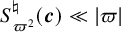


Proof. Part (1) is due to Hooley [Reference Hooley32, Lemma 60]. Part (2) is straightforward and is recorded in the proof of [Reference Glas and Hochfilzer26, Eq. (4.7)], although we take the opportunity to correct the definition of
$\{\varpi ^e,c_i\}$
 to be equal to
$1$
to be equal to
$1$
 when
$e=2$
when
$e=2$
 . To see part (3) we invoke [Reference Glas and Hochfilzer26, Eq. (4.7)] to deduce that

where
$\{\varpi ^e,c_i\}=|\varpi |^{-1}$
 if
$\varpi \| c_i$
if
$\varpi \| c_i$
 , with
$\{\varpi ^e,c_i\}=|\gcd (\varpi ^e,c_i)|$
, with
$\{\varpi ^e,c_i\}=|\gcd (\varpi ^e,c_i)|$
 otherwise. The statement of the lemma follows on noting that
$\{\varpi ^e,c_i\}\leqslant |\gcd (\varpi ^e,\operatorname {\mathrm {sq}}(c_i))|$
otherwise. The statement of the lemma follows on noting that
$\{\varpi ^e,c_i\}\leqslant |\gcd (\varpi ^e,\operatorname {\mathrm {sq}}(c_i))|$
 .
.
The following result follows from combining Lemma 6.1 with multiplicativity.
Lemma 6.2. There exists a constant
$A>0$
 such that

It will also be useful to record a crude upper bound, which will be helpful when
$\boldsymbol {c}=\boldsymbol {0}$
 .
.
Lemma 6.3. There exists a constant
$A>0$
 such that

Proof. By multiplicativity, it suffices to show that
$ S_{\varpi ^e}^\natural ({\boldsymbol {c}}) \ll |\varpi ^e|^{1/2+\theta _e}$
 , for any prime power
$\varpi ^e\in \mathcal {O}$
, for any prime power
$\varpi ^e\in \mathcal {O}$
 , where

For
$e\leqslant 2$
 this follows from parts (1) and (2) of Lemma 6.1. For
$e\geqslant 3$
this follows from parts (1) and (2) of Lemma 6.1. For
$e\geqslant 3$
 , we apply the
$1$
, we apply the
$1$
 -dimensional Hua type estimate recorded in [Reference Glas and Hochfilzer26, § 4.2].
The following classical recursive structure will soon prove useful.
Lemma 6.4. If
$\varpi \mid \boldsymbol {c}$
 and
$e\geqslant 4$
and
$e\geqslant 4$
 , then

Proof. After expressing
$S_{\varpi ^e}(\boldsymbol {c})$
 in terms of one-dimensional sums, this is immediate from the function field analogues of [Reference Hooley29, Eq. (44)–(45)], which hold since
$\operatorname {\mathrm {char}}(\mathbb {F}_q)\ne 3$
in terms of one-dimensional sums, this is immediate from the function field analogues of [Reference Hooley29, Eq. (44)–(45)], which hold since
$\operatorname {\mathrm {char}}(\mathbb {F}_q)\ne 3$
 .
.
Since a priori (depending on one’s conventionFootnote 2 ) the dual form is only defined up to scaling, and we will soon need to understand its relation to discriminants from work of Busé and Jouanolou [Reference Busé and Jouanolou14, Definition 4.6], we record the following standard fact.
Proposition 6.5. Let
$R=\mathbb {F}_q[c_1,\dots ,c_{n-1}]$
 . Then
$F^\ast (c_1,\dots ,c_{n-1},1) \in R$
. Then
$F^\ast (c_1,\dots ,c_{n-1},1) \in R$
 is divisible by the discriminant
$\Delta \in R$
is divisible by the discriminant
$\Delta \in R$
 of the cubic form

Proof. Here
$\Delta $
 is defined by a specialisation process explained in [Reference Busé and Jouanolou14, paragraph after Eq. (4.2.1)]. Write
$\boldsymbol {c}=(c_1,\dots ,c_{n-1},1)$
is defined by a specialisation process explained in [Reference Busé and Jouanolou14, paragraph after Eq. (4.2.1)]. Write
$\boldsymbol {c}=(c_1,\dots ,c_{n-1},1)$
 and let
$\operatorname {\mathrm {disc}}(F,\boldsymbol {c})$
and let
$\operatorname {\mathrm {disc}}(F,\boldsymbol {c})$
 be the discriminant associated in [Reference Terakado50, § 1.1] to the pair
$(F(\boldsymbol {x}), \boldsymbol {c}\cdot \boldsymbol {x})$
be the discriminant associated in [Reference Terakado50, § 1.1] to the pair
$(F(\boldsymbol {x}), \boldsymbol {c}\cdot \boldsymbol {x})$
 .
.
As explained in [Reference Wang53, Proposition 4.4], for example, we have
$\operatorname {\mathrm {disc}}(F,\boldsymbol {c}) / F^\ast (\boldsymbol {c}) \in \mathbb {F}_q^\times $
 . (This is the only step where we use
$\operatorname {\mathrm {char}}(\mathbb {F}_q)> 3$
. (This is the only step where we use
$\operatorname {\mathrm {char}}(\mathbb {F}_q)> 3$
 .) Also

by [Reference Wang53, Proposition 3.2]. It therefore follows that
$\Delta / F^\ast \in \mathbb {F}_q^\times $
 , which suffices.
The following result is the function field analogue of [Reference Wang57, Lemma 9.1 (2),(3)].
Lemma 6.6. Let
$\varpi ^e\in \mathcal {O}$
 be a prime power.
-
1. If $e=2$
and
$v_\varpi (F^*({\boldsymbol {c}}))\leqslant 1$
then
$S_{\varpi ^2}^\natural (\boldsymbol {c})\ll 1$
. -
2. If $e\geqslant 2+v_\varpi (F^*({\boldsymbol {c}}))$
then
$S_{\varpi ^e}(\boldsymbol {c})=0$
.


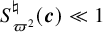


Proof. Let
$e>1$
 and assume that
$\varpi \nmid {\boldsymbol {c}}$
and assume that
$\varpi \nmid {\boldsymbol {c}}$
 . We may appeal to an argument of Hooley [Reference Hooley34, § 6], which carries over to the function field setting to give

Here, for
$i\in \{0,1\}$
 ,
$\nu _i(\varpi ^e,{\boldsymbol {c}})$
,
$\nu _i(\varpi ^e,{\boldsymbol {c}})$
 is the number of
$\boldsymbol {y}\bmod {\varpi ^e}$
is the number of
$\boldsymbol {y}\bmod {\varpi ^e}$
 such that
$F(\boldsymbol {y})\equiv 0\bmod {\varpi ^e}$
such that
$F(\boldsymbol {y})\equiv 0\bmod {\varpi ^e}$
 , with
$\varpi \nmid \boldsymbol {y}$
, with
$\varpi \nmid \boldsymbol {y}$
 and
${\boldsymbol {c}}.\boldsymbol {y}\equiv 0\bmod {\varpi ^{e-i}}$
and
${\boldsymbol {c}}.\boldsymbol {y}\equiv 0\bmod {\varpi ^{e-i}}$
 . Since F is a nonsingular cubic form with coefficients in
$\mathbb {F}_q$
. Since F is a nonsingular cubic form with coefficients in
$\mathbb {F}_q$
 , it follows that
$\varpi \nmid \nabla F(\boldsymbol {y})$
, it follows that
$\varpi \nmid \nabla F(\boldsymbol {y})$
 for any
$\boldsymbol {y}$
for any
$\boldsymbol {y}$
 such that
$\varpi \mid F(\boldsymbol {y})$
such that
$\varpi \mid F(\boldsymbol {y})$
 but
$\varpi \nmid \boldsymbol {y}$
but
$\varpi \nmid \boldsymbol {y}$
 . Hence
$\nu _1(\varpi ^e,{\boldsymbol {c}})=|\varpi |^{n-1}\nu _0(\varpi ^{e-1},{\boldsymbol {c}})$
. Hence
$\nu _1(\varpi ^e,{\boldsymbol {c}})=|\varpi |^{n-1}\nu _0(\varpi ^{e-1},{\boldsymbol {c}})$
 , so that

Since
$\varpi \nmid {\boldsymbol {c}}$
 , we can assume without loss of generality that
$\varpi \nmid c_n$
, we can assume without loss of generality that
$\varpi \nmid c_n$
 . Eliminating
$y_n$
. Eliminating
$y_n$
 , we are left with the expression

where
$\nu (\varpi ^e,{\boldsymbol {c}})$
 is the number of
$\boldsymbol {y}'=(y_1,\dots ,y_{n-1})\bmod {\varpi ^e}$
is the number of
$\boldsymbol {y}'=(y_1,\dots ,y_{n-1})\bmod {\varpi ^e}$
 such that
$G(\boldsymbol {y}')\equiv 0\bmod {\varpi ^e}$
such that
$G(\boldsymbol {y}')\equiv 0\bmod {\varpi ^e}$
 and
$\varpi \nmid \boldsymbol {y}'$
and
$\varpi \nmid \boldsymbol {y}'$
 , where
$ G(\boldsymbol {y}')=F(c_ny_1,\dots ,c_ny_{n-1},-c_1y_1-\dots -c_{n-1}y_{n-1}). $
, where
$ G(\boldsymbol {y}')=F(c_ny_1,\dots ,c_ny_{n-1},-c_1y_1-\dots -c_{n-1}y_{n-1}). $
 Part (2) for
$\varpi \nmid \boldsymbol {c}$
Part (2) for
$\varpi \nmid \boldsymbol {c}$
 now follows from taking
$m=e-1$
now follows from taking
$m=e-1$
 ,
$\delta \in [0, \tfrac {m-1}{2}]$
,
$\delta \in [0, \tfrac {m-1}{2}]$
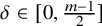 and
$\ell =0$
and
$\ell =0$
 in the multivariate form of the Hensel-type lemma [Reference Browning and Matthiesen11, Lemma 3.3], carried over to
$\mathcal {O}$
in the multivariate form of the Hensel-type lemma [Reference Browning and Matthiesen11, Lemma 3.3], carried over to
$\mathcal {O}$
 . Indeed, for any
$\boldsymbol {u}'$
. Indeed, for any
$\boldsymbol {u}'$
 counted by
$\nu (\varpi ^{e-1},{\boldsymbol {c}})$
counted by
$\nu (\varpi ^{e-1},{\boldsymbol {c}})$
 , we must have

or else
$v_\varpi (F^\ast (\boldsymbol {c})) \geqslant e-1$
 by the
$\beta = \lceil \frac {e-1}{2} \rceil $
by the
$\beta = \lceil \frac {e-1}{2} \rceil $
 case of Lemma 6.7. Using Lemma 6.4 and arguing by induction on
$v_\varpi (\boldsymbol {c})$
case of Lemma 6.7. Using Lemma 6.4 and arguing by induction on
$v_\varpi (\boldsymbol {c})$
 , we can also conclude that part (2) holds if
$\varpi \mid \boldsymbol {c}$
, we can also conclude that part (2) holds if
$\varpi \mid \boldsymbol {c}$
 .
.
Turning to part (1), we take
$e=2$
 and note that
$\varpi \nmid {\boldsymbol {c}}$
and note that
$\varpi \nmid {\boldsymbol {c}}$
 if
$v_\varpi (F^*({\boldsymbol {c}}))\leqslant 1$
if
$v_\varpi (F^*({\boldsymbol {c}}))\leqslant 1$
 , since
$\deg F^*>1$
, since
$\deg F^*>1$
 . But then it follows that

Pick
$\boldsymbol {u}'$
 counted by
$\nu (\varpi ,{\boldsymbol {c}})$
counted by
$\nu (\varpi ,{\boldsymbol {c}})$
 . If
$\varpi \nmid \nabla G(\boldsymbol {u}')$
. If
$\varpi \nmid \nabla G(\boldsymbol {u}')$
 then the contribution to the right hand side vanishes, by Hensel lifting. On the other hand, if
$\varpi \mid \nabla G(\boldsymbol {u}')$
then the contribution to the right hand side vanishes, by Hensel lifting. On the other hand, if
$\varpi \mid \nabla G(\boldsymbol {u}')$
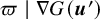 then Lemma 6.7 implies that the contribution to
$\nu (\varpi ^2,{\boldsymbol {c}})$
then Lemma 6.7 implies that the contribution to
$\nu (\varpi ^2,{\boldsymbol {c}})$
 vanishes. Hence

It follows from a result of Zak [Reference Hooley31, Katz’s Appendix, Theorem 2] that the hypersurface
$G=0$
 in
$\mathbb {P}^{n-2}$
in
$\mathbb {P}^{n-2}$
 has only
$O(1)$
has only
$O(1)$
 singular points, whence the number of
$\boldsymbol {u}'$
singular points, whence the number of
$\boldsymbol {u}'$
 is
$O(|\varpi |)$
is
$O(|\varpi |)$
 . It follows that

which is what we wanted.
Lemma 6.7. Suppose
$\varpi \nmid \boldsymbol {u}'$
 and
$\varpi ^\beta \mid \nabla G(\boldsymbol {u}')$
and
$\varpi ^\beta \mid \nabla G(\boldsymbol {u}')$
 . Then
$v_\varpi (F^*({\boldsymbol {c}})) \geqslant \min (v_\varpi (G(\boldsymbol {u}')), 2\beta )$
. Then
$v_\varpi (F^*({\boldsymbol {c}})) \geqslant \min (v_\varpi (G(\boldsymbol {u}')), 2\beta )$
 .
.
Proof. Since
$\varpi \nmid \boldsymbol {u}'$
 , we have
$\varpi \nmid u_a$
, we have
$\varpi \nmid u_a$
 , say. Then by Proposition 6.5 and [Reference Busé and Jouanolou14, Corollary 4.30; see the beginning of § 4 for the definition of
$\tilde{f}$
, say. Then by Proposition 6.5 and [Reference Busé and Jouanolou14, Corollary 4.30; see the beginning of § 4 for the definition of
$\tilde{f}$
 there],
$F^\ast (\boldsymbol {c})$
there],
$F^\ast (\boldsymbol {c})$
 is an
$\mathcal {O}[\boldsymbol {u}'][1/u_a]$
is an
$\mathcal {O}[\boldsymbol {u}'][1/u_a]$
 -linear combination of G and the pairwise products
$(\partial G/\partial u_i)(\partial G/\partial u_j)$
-linear combination of G and the pairwise products
$(\partial G/\partial u_i)(\partial G/\partial u_j)$
 . Since
$\varpi ^{2\beta }$
. Since
$\varpi ^{2\beta }$
 divides each pairwise product, the desired divisibility of
$F^\ast (\boldsymbol {c})$
divides each pairwise product, the desired divisibility of
$F^\ast (\boldsymbol {c})$
 follows.
In addition, we have the following estimate for averages over moduli belonging to
$\mathcal {R}_{\boldsymbol {c}}^{\text {B}}$
 , which is a consequence of Lemma 4.4 in [Reference Glas and Hochfilzer26] and (6.8) in [Reference Glas and Hochfilzer26], together with the bound
$\#\mathcal {R}(\mathbf {C})\ll \widehat C^n$
, which is a consequence of Lemma 4.4 in [Reference Glas and Hochfilzer26] and (6.8) in [Reference Glas and Hochfilzer26], together with the bound
$\#\mathcal {R}(\mathbf {C})\ll \widehat C^n$
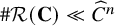 .
.
Proposition 6.8. Let
$Y, C \geqslant 1$
 . Then

We end by recalling [Reference Glas and Hochfilzer26, Lemma 4.2] (a special case of [Reference Browning and Vishe12, Lemma 8.5]), which concerns square-root cancellation of
$S_r(\boldsymbol {c})$
 over ‘good’ moduli r.
Proposition 6.9. Let
$Y\geqslant 1$
 and
$\boldsymbol {c}\in \mathcal {S}_1$
and
$\boldsymbol {c}\in \mathcal {S}_1$
 . Then

7 Moments of bad exponential sums
Our primary goal in this section is to prove the following result.
Theorem 7.1. Let
$0\leqslant R\leqslant 3Z$
 . There exist
$\eta ,\delta>0$
. There exist
$\eta ,\delta>0$
 such that if
$2\leqslant A\leqslant 2+\delta $
such that if
$2\leqslant A\leqslant 2+\delta $
 , then
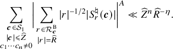
(As we will see in § 8, the complementary locus
$\{\boldsymbol {c}\in \mathcal {S}_1: c_1\cdots c_n=0\}$
 has essentially already been satisfactorily treated in [Reference Glas and Hochfilzer26].)
Let us denote by
$\Sigma _A=\Sigma _A(Z,R)$
 the sum on the left-hand side in the statement of this result. The trivial bounds
$\lvert S_r(\boldsymbol {c}) \rvert \leqslant \lvert r \rvert ^{1+n}$
the sum on the left-hand side in the statement of this result. The trivial bounds
$\lvert S_r(\boldsymbol {c}) \rvert \leqslant \lvert r \rvert ^{1+n}$
 and
$\#\{r\in \mathcal {R}_{\boldsymbol {c}}^{\text {B}}: \lvert r \rvert =\widehat R\} \leqslant \widehat R$
and
$\#\{r\in \mathcal {R}_{\boldsymbol {c}}^{\text {B}}: \lvert r \rvert =\widehat R\} \leqslant \widehat R$
 imply
imply

To analyse
$\Sigma _2$
 , it will be convenient to define

and

Following the approach in [Reference Wang57, § 9], we shall use different arguments according to the size of
$T_r({\boldsymbol {c}})$
 . Let
$B\geqslant 0$
. Let
$B\geqslant 0$
 be a parameter to be chosen in due course and note that
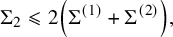
where
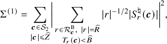

7.1 Ekedahl sieve
A version of the geometric sieve for arbitrary global fields has been worked out by Bhargava, Shankar and Wang [Reference Bhargava, Shankar and Wang7]. Their result sieves out prime moduli, but we need at least a partial version of the result for square-free moduli. This is folklore but we prove it for the reader’s convenience. A similar idea is used in [Reference Bhargava6, § 5, Case III].
Theorem 7.2. Let
$T,Y>0$
 . Fix two polynomials
$H_0,H_1\in \mathcal {O}[c_1,\dots ,c_n]$
. Fix two polynomials
$H_0,H_1\in \mathcal {O}[c_1,\dots ,c_n]$
 that are relatively prime in
$K[c_1,\dots ,c_n]$
that are relatively prime in
$K[c_1,\dots ,c_n]$
 . Then

Proof.
Case 1:
$Y\leqslant T$
 . Applying the Lang–Weil estimate for the quasi-projective variety
$H_0=H_1=0$
. Applying the Lang–Weil estimate for the quasi-projective variety
$H_0=H_1=0$
 , the count on the left is seen to be
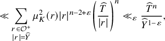
as desired.
Case 2:
$Y>T$
 . By Lemma 2.7, we can make an
$\mathcal {O}$
. By Lemma 2.7, we can make an
$\mathcal {O}$
 -linear change of variables in order to assume that
$\deg _{c_1}(H_0) = \deg (H_0)$
-linear change of variables in order to assume that
$\deg _{c_1}(H_0) = \deg (H_0)$
 and
$\deg _{c_1}(H_1) = \deg (H_1)$
and
$\deg _{c_1}(H_1) = \deg (H_1)$
 .
.
Let
$H_2\in \mathcal {O}[c_2,\dots ,c_n]$
 be the resultant of
$H_0$
be the resultant of
$H_0$
 and
$H_1$
and
$H_1$
 with respect to
$c_1$
with respect to
$c_1$
 . Then any square-free
$r\in \mathcal {O}^+$
. Then any square-free
$r\in \mathcal {O}^+$
 such that
$r\mid \gcd (H_0(\boldsymbol {c}), H_1(\boldsymbol {c}))$
such that
$r\mid \gcd (H_0(\boldsymbol {c}), H_1(\boldsymbol {c}))$
 must also satisfyFootnote
3
must also satisfyFootnote
3

If
$c_2,\dots ,c_n\in \mathcal {O}$
 are specified, with
$|c_2|,\dots ,|c_n|\ll \widehat T$
are specified, with
$|c_2|,\dots ,|c_n|\ll \widehat T$
 , then either
$H_2(c_2,\dots ,c_n) = 0$
, then either
$H_2(c_2,\dots ,c_n) = 0$
 or else there are only
$O_\varepsilon (\widehat T^\varepsilon )$
or else there are only
$O_\varepsilon (\widehat T^\varepsilon )$
 choices for
$r\mid H_2(c_2,\dots ,c_n)$
choices for
$r\mid H_2(c_2,\dots ,c_n)$
 , by the divisor function bound. Note that if r is also specified, then the number of choices for
$c_1\in \mathcal {O}$
, by the divisor function bound. Note that if r is also specified, then the number of choices for
$c_1\in \mathcal {O}$
 with
$|c_1|\ll \widehat T$
with
$|c_1|\ll \widehat T$
 and
$r\mid H_0(\boldsymbol {c})$
and
$r\mid H_0(\boldsymbol {c})$
 is
is
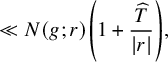
in the notation of (2.21), where
$g(u)=H_0(u,c_2,\dots ,c_n)$
 . It follows from (2.23) that
$N(g;r)\ll _\varepsilon |r|^{\varepsilon }$
. It follows from (2.23) that
$N(g;r)\ll _\varepsilon |r|^{\varepsilon }$
 , uniformly over
$c_2,\dots ,c_n\in \mathcal {O}$
, uniformly over
$c_2,\dots ,c_n\in \mathcal {O}$
 .
.
Putting everything together, and recalling that
$Y>T$
 , we obtain the overall contribution

Since
$H_0$
 and
$H_1$
and
$H_1$
 are coprime over K, it follows that
$H_2$
are coprime over K, it follows that
$H_2$
 is a nonzero polynomial, whence the first term is
$O(\widehat T^{n-1})$
is a nonzero polynomial, whence the first term is
$O(\widehat T^{n-1})$
 by Lemma 2.10.
7.2 Treatment of
$\Sigma^{(1)}$

The main task of this section is to prove the following result.
Proposition 7.3. Let
$0\leqslant R\leqslant 3Z$
 and let
$B\geqslant 0$
and let
$B\geqslant 0$
 . Then

where
$\eta _0=\min \{1/p,1/(3\cdot 2^{n+1})\}$
 and
$p=\operatorname {\mathrm {char}}(\mathbb {F}_q)$
and
$p=\operatorname {\mathrm {char}}(\mathbb {F}_q)$
 .
.
Recall the definition (7.3) of
$\Sigma ^{(1)}$
 . Any
$r\in \mathcal {R}_{\boldsymbol {c}}^{\text {B}}$
. Any
$r\in \mathcal {R}_{\boldsymbol {c}}^{\text {B}}$
 admits a factorisation
$r=r_1s_1s_2$
admits a factorisation
$r=r_1s_1s_2$
 , where
$r_1,s_1,s_2$
, where
$r_1,s_1,s_2$
 are relatively coprime such that
$r_1$
are relatively coprime such that
$r_1$
 is square-free and
$s_1,s_2$
is square-free and
$s_1,s_2$
 are both square-full, and satisfy

It follows from parts (1)–(2) of Lemma 6.6 that
$S_{s_1}^\natural ({\boldsymbol {c}})\ll _\varepsilon |s_1|^\varepsilon $
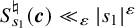 for any
$\varepsilon>0$
for any
$\varepsilon>0$
 . On the other hand, from the definition of
$s_2$
. On the other hand, from the definition of
$s_2$
 we have
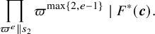
Moreover, it is clear that the left hand side is a square-full element of
$\mathcal {O}$
 with absolute value
$ \prod _{\varpi ^e\| s_2} |\varpi |^{\text {max}\{2,e-1\}}\geqslant |s_2|^{2/3}. $
with absolute value
$ \prod _{\varpi ^e\| s_2} |\varpi |^{\text {max}\{2,e-1\}}\geqslant |s_2|^{2/3}. $
 We note that
$\text {max}\{|r_1|,|s_1|,|s_2|\}\geqslant |r|^{1/3}=\widehat R^{1/3}.$
We note that
$\text {max}\{|r_1|,|s_1|,|s_2|\}\geqslant |r|^{1/3}=\widehat R^{1/3}.$
 Let us temporarily write
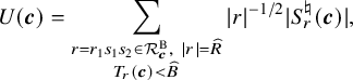
so that
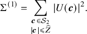
We will argue differently according to which of
$|r_1|,|s_1|,|s_2|$
 is the maximum in the factorisation
$r=r_1s_1s_2$
is the maximum in the factorisation
$r=r_1s_1s_2$
 , exploiting the multiplicativity of the sum
$S^\natural _r(\boldsymbol {c})$
, exploiting the multiplicativity of the sum
$S^\natural _r(\boldsymbol {c})$
 .
.
The contribution to
$U({\boldsymbol {c}})$
 from the case
$\text {max}\{|r_1|,|s_1|,|s_2|\}=|r_1|$
from the case
$\text {max}\{|r_1|,|s_1|,|s_2|\}=|r_1|$
 is
is

since
$ |s_1s_2|^{-1/2} |S^\natural _{s_1s_2}(\boldsymbol {c})|\leqslant T_{s_1s_2}({\boldsymbol {c}})\leqslant T_{r}({\boldsymbol {c}})<\widehat B, $
 by assumption. It follows from Lemma 2.2 that the number of available
$s_1,s_2$
by assumption. It follows from Lemma 2.2 that the number of available
$s_1,s_2$
 is
$O_\varepsilon (\widehat Z^\varepsilon )$
is
$O_\varepsilon (\widehat Z^\varepsilon )$
 , on recalling that
$F^*({\boldsymbol {c}})\neq 0$
, on recalling that
$F^*({\boldsymbol {c}})\neq 0$
 and
$R\leqslant 3Z$
and
$R\leqslant 3Z$
 . Hence the overall contribution to
$\Sigma ^{(1)}$
. Hence the overall contribution to
$\Sigma ^{(1)}$
 from this case is
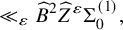
where
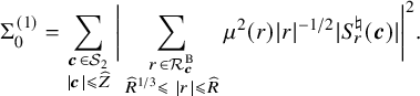
Next, the contribution to
$U({\boldsymbol {c}})$
 from the case
$\text {max}\{|r_1|,|s_1|,|s_2|\}=|s_1|$
from the case
$\text {max}\{|r_1|,|s_1|,|s_2|\}=|s_1|$
 is
is
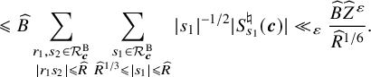
Finally, the contribution to
$U({\boldsymbol {c}})$
 from the case
$\text {max}\{|r_1|,|s_1|,|s_2|\}=|s_2|$
from the case
$\text {max}\{|r_1|,|s_1|,|s_2|\}=|s_2|$
 is
is

where

Putting everything together, it now follows that

where

The statement of Proposition 7.3 now follows from the conjunction of the following pair of results, both of which rely on the version of the geometric sieve for function fields from § 7.1.
Lemma 7.4. We have
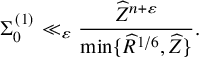
Lemma 7.5. We have

where p is the characteristic of
$\mathbb {F}_q$
 .
.
Proof of Lemma 7.4
It follows from multiplicativity and Lemma 6.1(1) that

We pick a parameter
$0\leqslant Y\leqslant R$
 and break the set
$\mathcal {S}_2$
and break the set
$\mathcal {S}_2$
 into two sets

To begin with, if
${\boldsymbol {c}}\in \mathcal {S}_{2,1}$
 then we take
$S_r^\natural ({\boldsymbol {c}})\ll _\varepsilon \widehat Z^\varepsilon |r|^{1/2}$
then we take
$S_r^\natural ({\boldsymbol {c}})\ll _\varepsilon \widehat Z^\varepsilon |r|^{1/2}$
 and we note that there are
$O_\varepsilon (\widehat Z^\varepsilon )$
and we note that there are
$O_\varepsilon (\widehat Z^\varepsilon )$
 choices of r, by Lemma 2.2. On the other hand, if
${\boldsymbol {c}}\in \mathcal {S}_{2,2}$
choices of r, by Lemma 2.2. On the other hand, if
${\boldsymbol {c}}\in \mathcal {S}_{2,2}$
 then we may take
$S_r^\natural ({\boldsymbol {c}})\ll _\varepsilon \widehat Z^\varepsilon \widehat Y^{1/2}$
then we may take
$S_r^\natural ({\boldsymbol {c}})\ll _\varepsilon \widehat Z^\varepsilon \widehat Y^{1/2}$
 and we also have
$O_\varepsilon (\widehat Z^\varepsilon )$
and we also have
$O_\varepsilon (\widehat Z^\varepsilon )$
 choices of r overall. It follows that
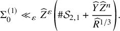
Since
$3\cdot 2^{n-2} F^\ast = \boldsymbol {c}\cdot \nabla {F^\ast }$
 , we can apply the geometric sieve, in the form of Theorem 7.2 (with
$H_0 = F^\ast $
, we can apply the geometric sieve, in the form of Theorem 7.2 (with
$H_0 = F^\ast $
 and
$H_1 = \partial {F^\ast }/\partial {c_1}$
and
$H_1 = \partial {F^\ast }/\partial {c_1}$
 , noting that
$F^\ast $
, noting that
$F^\ast $
 is absolutely irreducible and
$\deg {H_1}<\deg {H_0}$
is absolutely irreducible and
$\deg {H_1}<\deg {H_0}$
 ), in order to deduce the bound
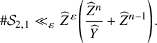
The statement of the lemma follows on combining these and taking
$Y=\frac {1}{6}R$
 .
.
Proof of Lemma 7.5
We shall reduce the problem to estimating the quantities

and

for suitable
$M_1,M_2\geqslant 0$
 .
.
Let
$\boldsymbol {c}\in \mathcal {O}^n$
 be counted by
$N(M,R)$
be counted by
$N(M,R)$
 , so that
$\lvert \boldsymbol {c} \rvert \leqslant \widehat Z$
, so that
$\lvert \boldsymbol {c} \rvert \leqslant \widehat Z$
 and
$c_1\dots c_n F^*({\boldsymbol {c}})\neq 0$
and
$c_1\dots c_n F^*({\boldsymbol {c}})\neq 0$
 , and there exists a square-full
$d\in \mathcal {O}$
, and there exists a square-full
$d\in \mathcal {O}$
 such that
$d\mid F^*({\boldsymbol {c}})$
such that
$d\mid F^*({\boldsymbol {c}})$
 and
$|d|=\widehat M$
and
$|d|=\widehat M$
 . Any such d admits a factorisation

where
$e_1,\dots ,e_m\geqslant 2$
 . Let
$\eta \in (0,1]$
. Let
$\eta \in (0,1]$
 be a parameter, to be chosen in due course. Suppose first that
$|\varpi _i^{e_i}|\leqslant \widehat Z^\eta $
be a parameter, to be chosen in due course. Suppose first that
$|\varpi _i^{e_i}|\leqslant \widehat Z^\eta $
 for all
$1\leqslant i\leqslant m$
for all
$1\leqslant i\leqslant m$
 . Then we claim that
${\boldsymbol {c}}$
. Then we claim that
${\boldsymbol {c}}$
 is counted by

To see this, if
$M\leqslant Z$
 then in fact
${\boldsymbol {c}}$
then in fact
${\boldsymbol {c}}$
 is counted by
$N_1(M,Z)$
is counted by
$N_1(M,Z)$
 , which is satisfactory since

If
$M>Z$
 then we consider the square-full integer
$d_1=d/\varpi _1^{e_1}$
then we consider the square-full integer
$d_1=d/\varpi _1^{e_1}$
 , with absolute value
$|d_1|=\widehat M/|\varpi _1^{e_1}|\geqslant \widehat M/\widehat Z^\eta $
, with absolute value
$|d_1|=\widehat M/|\varpi _1^{e_1}|\geqslant \widehat M/\widehat Z^\eta $
 . If
$\widehat M/|\varpi _1^{e_1}|\leqslant \widehat Z$
. If
$\widehat M/|\varpi _1^{e_1}|\leqslant \widehat Z$
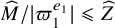 then
${\boldsymbol {c}}$
then
${\boldsymbol {c}}$
 is counted by
$N_1(M-\eta Z ,Z)$
is counted by
$N_1(M-\eta Z ,Z)$
 , where

On the other hand, if
$\widehat M/|\varpi _1^{e_1}|> \widehat Z$
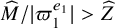 then we repeat the argument for
$d_2=d_1/\varpi _2^{e_2}$
then we repeat the argument for
$d_2=d_1/\varpi _2^{e_2}$
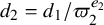 . The claim follows on continuing in this way, since the process clearly terminates with a square-full divisor in the desired interval.
We now suppose, by symmetry, that
$|\varpi _1^{e_1}|> \widehat Z^\eta $
 . If
$|\varpi _1|\leqslant \widehat Z^{\eta /2}$
. If
$|\varpi _1|\leqslant \widehat Z^{\eta /2}$
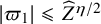 then we let
$e_1'\leqslant e_1$
then we let
$e_1'\leqslant e_1$
 be the largest integer such that
$|\varpi _1^{e_1'}|\leqslant \widehat Z^\eta $
be the largest integer such that
$|\varpi _1^{e_1'}|\leqslant \widehat Z^\eta $
 . It then follows that
$|\varpi _1^{e_1'+1}|> \widehat Z^\eta $
. It then follows that
$|\varpi _1^{e_1'+1}|> \widehat Z^\eta $
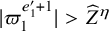 , whence
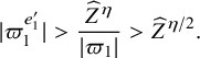
Moreover, we must have
$e_1'\geqslant 2$
 since
$|\varpi _1|\leqslant \widehat Z^{\eta /2}$
since
$|\varpi _1|\leqslant \widehat Z^{\eta /2}$
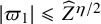 . Thus, since
$\eta \leqslant 1$
. Thus, since
$\eta \leqslant 1$
 , we see that
$\varpi _1^{e_1'}$
, we see that
$\varpi _1^{e_1'}$
 is a square-full divisor of
$F^*({\boldsymbol {c}})$
is a square-full divisor of
$F^*({\boldsymbol {c}})$
 whose norm lies in the interval
$(\widehat Z^{\eta /2},\widehat Z]$
whose norm lies in the interval
$(\widehat Z^{\eta /2},\widehat Z]$
 . In this case, therefore, we deduce that
${\boldsymbol {c}}$
. In this case, therefore, we deduce that
${\boldsymbol {c}}$
 is counted by
$N_1(\frac {\eta }{2}Z ,Z)$
is counted by
$N_1(\frac {\eta }{2}Z ,Z)$
 . Finally, we must attend to the case that
$|\varpi _1^{e_1}|> \widehat Z^\eta $
. Finally, we must attend to the case that
$|\varpi _1^{e_1}|> \widehat Z^\eta $
 and
$|\varpi _1|> \widehat Z^{\eta /2}$
and
$|\varpi _1|> \widehat Z^{\eta /2}$
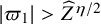 . But then it is immediate that
${\boldsymbol {c}}$
. But then it is immediate that
${\boldsymbol {c}}$
 is counted by
$N_2(\frac {\eta }{2}Z ,Z)$
is counted by
$N_2(\frac {\eta }{2}Z ,Z)$
 .
.
In summary, we may conclude that

for any
$\eta \in (0,1]$
 . We claim that
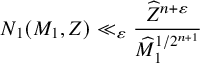
and
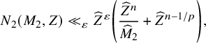
for any
$M_1,M_2>0$
 , where p is the characteristic of
$\mathbb {F}_q$
, where p is the characteristic of
$\mathbb {F}_q$
 . Applying these in (7.5), we deduce that

since
$\eta \min \{M,Z\}\leqslant \eta Z$
 . The statement of Lemma 7.5 easily follows on taking
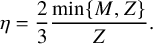
Treatment of
$N_1(M_1,Z)$

We will only make
$N_1(M_1,Z)$
 bigger by summing over all possible square-full d, and then breaking into residue classes modulo d. This gives
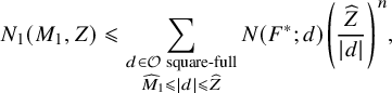
in the notation of (2.21). Let
$\delta =2^{-n}.$
 Since
$N(F^*;d)$
Since
$N(F^*;d)$
 is multiplicative in d, it follows from Rankin’s trick that

When
$e=2$
 , we have
$N(F^\ast ;\varpi ^2) = O(|\varpi |^{2n-2})$
, we have
$N(F^\ast ;\varpi ^2) = O(|\varpi |^{2n-2})$
 by Lemma 2.9. It follows that

Once combined with Corollary 2.8, we conclude that

since
$F^*$
 is an absolutely irreducible form of degree
$3\times 2^{n-2}\leqslant 2^n$
is an absolutely irreducible form of degree
$3\times 2^{n-2}\leqslant 2^n$
 . But clearly

since
$\delta =2^{-n}$
 . Thus the product over
$\varpi $
. Thus the product over
$\varpi $
 converges absolutely and the bound (7.6) follows on noting that
$\widehat M_1^\varepsilon \leqslant \widehat Z^\varepsilon $
converges absolutely and the bound (7.6) follows on noting that
$\widehat M_1^\varepsilon \leqslant \widehat Z^\varepsilon $
 .
.
Treatment of
$N_2(M_2,Z)$

We follow the argument in Poonen [Reference Poonen45, § 7], noting that
$F^*$
 is a square-free polynomial defined over
$\mathbb {F}_q$
is a square-free polynomial defined over
$\mathbb {F}_q$
 . Poonen defines the polynomial
$G\in \mathcal {O}[(y_{i,j})_{1\leqslant i\leqslant n, 0\leqslant j\leqslant p-1}]$
. Poonen defines the polynomial
$G\in \mathcal {O}[(y_{i,j})_{1\leqslant i\leqslant n, 0\leqslant j\leqslant p-1}]$
 via
via

where p is the characteristic of
$\mathbb {F}_q$
 . It follows from n applications of [Reference Poonen45, Lemma 7.2] that G is square-free as an element of
$K[y_{i,j}]$
. It follows from n applications of [Reference Poonen45, Lemma 7.2] that G is square-free as an element of
$K[y_{i,j}]$
 . Let
$Z_j=(Z-j)/p$
. Let
$Z_j=(Z-j)/p$
 . Then, as
$y_{i,j}$
. Then, as
$y_{i,j}$
 runs over elements of
$\mathcal {O}$
runs over elements of
$\mathcal {O}$
 with
$|y_{i,j}|\leqslant \widehat Z_j$
with
$|y_{i,j}|\leqslant \widehat Z_j$
 , so the n-tuples
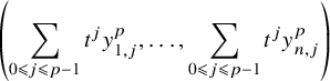
run over elements
$\mathbf {z}\in \mathcal {O}^n$
 with
$\lvert \mathbf {z} \rvert \leqslant \widehat Z$
with
$\lvert \mathbf {z} \rvert \leqslant \widehat Z$
 , with each element appearing exactly once. Hence it follows that

Poonen’s crucial observation is that we have
$\varpi \mid G(\boldsymbol {y})$
 and
$\varpi \mid G'(\boldsymbol {y})$
and
$\varpi \mid G'(\boldsymbol {y})$
 whenever
$\varpi ^2\mid G(\boldsymbol {y})$
whenever
$\varpi ^2\mid G(\boldsymbol {y})$
 , where
$G'=\frac {\partial G}{\partial t}$
, where
$G'=\frac {\partial G}{\partial t}$
 . Since G and
$G'$
. Since G and
$G'$
 are coprime as elements of
$K[y_{i,j}]$
are coprime as elements of
$K[y_{i,j}]$
 , by [Reference Poonen45, Lemma 7.3], we can therefore apply Theorem 7.2 to deduce that

since
$Z_j\leqslant Z_0\leqslant Z/p$
 for all
$0\leqslant j\leqslant p-1$
for all
$0\leqslant j\leqslant p-1$
 . This therefore establishes (7.7).
7.3 Treatment of
$\Sigma ^{(2)}$

We now turn to the estimation of
$\Sigma ^{(2)}$
 , as defined in (7.4), with the main goal being to prove the following bound.
Proposition 7.6. Let
$0\leqslant R\leqslant 3Z$
 and let
$B\geqslant 0$
and let
$B\geqslant 0$
 . Then
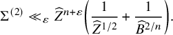
Proof. Let r and
${\boldsymbol {c}}$
 be counted by
$\Sigma ^{(2)}$
be counted by
$\Sigma ^{(2)}$
 . Then it follows from Lemma 6.2 that

since
$\operatorname {\mathrm {cub}}(s)\mid \operatorname {\mathrm {cub}}(r)$
 . On relabelling
$c_1,\dots ,c_n$
. On relabelling
$c_1,\dots ,c_n$
 , we may assume that the maximum occurs at
$i=n$
, we may assume that the maximum occurs at
$i=n$
 on the right hand side. According to part (2) of Lemma 6.6, moreover, we will have
$S^\natural _r(\boldsymbol {c})=0$
on the right hand side. According to part (2) of Lemma 6.6, moreover, we will have
$S^\natural _r(\boldsymbol {c})=0$
 unless
$e\leqslant 1+v_\varpi (F^*({\boldsymbol {c}}))$
unless
$e\leqslant 1+v_\varpi (F^*({\boldsymbol {c}}))$
 for any prime power
$\varpi ^e\|r$
for any prime power
$\varpi ^e\|r$
 . If we let
$d=\gcd (\operatorname {\mathrm {cub}}(r) , \operatorname {\mathrm {sq}}(c_n))$
. If we let
$d=\gcd (\operatorname {\mathrm {cub}}(r) , \operatorname {\mathrm {sq}}(c_n))$
 , then d is a square-full element of
$\mathcal {O}$
, then d is a square-full element of
$\mathcal {O}$
 with
with

Moreover,
$|d|\leqslant \widehat Z$
 since
$d\mid c_n$
since
$d\mid c_n$
 and
$c_n\neq 0$
and
$c_n\neq 0$
 . Finally, we note that
$d\mid F^*({\boldsymbol {c}})^2$
. Finally, we note that
$d\mid F^*({\boldsymbol {c}})^2$
 since
$d\mid \operatorname {\mathrm {cub}}(r)$
since
$d\mid \operatorname {\mathrm {cub}}(r)$
 and
$e\leqslant 2(e-1)$
and
$e\leqslant 2(e-1)$
 for
$e\geqslant 2$
for
$e\geqslant 2$
 .
.
Let
$D\in \mathbb {R}$
 be such that
$\widehat D=\widehat B^{4/n}/\widehat R^\varepsilon $
be such that
$\widehat D=\widehat B^{4/n}/\widehat R^\varepsilon $
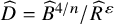 . Then we have proved that

since Lemma 2.2 implies that
$\#\{r\in \mathcal {R}_{\boldsymbol {c}}^{\text {B}}: \lvert r \rvert =\widehat R\}\ll _\varepsilon \widehat Z^\varepsilon $
 . In dealing with this sum we shall make frequent use of the bound
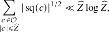
which readily follows on making the factorisation
$c=c_0\operatorname {\mathrm {sq}}(c)$
 , where
$c_0$
, where
$c_0$
 is the square-free part of c, and noting that there are
$O(\widehat C^{1/2})$
is the square-free part of c, and noting that there are
$O(\widehat C^{1/2})$
 square-full elements of
$\mathcal {O}$
square-full elements of
$\mathcal {O}$
 with absolute value
$\widehat C$
with absolute value
$\widehat C$
 .
.
We proceed by sorting the vectors
${\boldsymbol {c}}$
 into two contributions. Let
${\boldsymbol {c}}'=(c_1,\dots ,c_{n-1})$
into two contributions. Let
${\boldsymbol {c}}'=(c_1,\dots ,c_{n-1})$
 and let
$G({\boldsymbol {c}}')= F^*(c_1,\dots ,c_{n-1},0)^2$
and let
$G({\boldsymbol {c}}')= F^*(c_1,\dots ,c_{n-1},0)^2$
 . We first deal with the contribution from those
${\boldsymbol {c}}$
. We first deal with the contribution from those
${\boldsymbol {c}}$
 for which
$G({\boldsymbol {c}}')\neq 0$
for which
$G({\boldsymbol {c}}')\neq 0$
 . In this case we invert the order of summation and observe that there are
$O_\varepsilon (\widehat Z^\varepsilon )$
. In this case we invert the order of summation and observe that there are
$O_\varepsilon (\widehat Z^\varepsilon )$
 choices of d for which
$d\mid G({\boldsymbol {c}}')$
choices of d for which
$d\mid G({\boldsymbol {c}}')$
 , by the standard estimate for the divisor function. Hence the contribution to
$\Sigma ^{(2)}$
, by the standard estimate for the divisor function. Hence the contribution to
$\Sigma ^{(2)}$
 from this case is
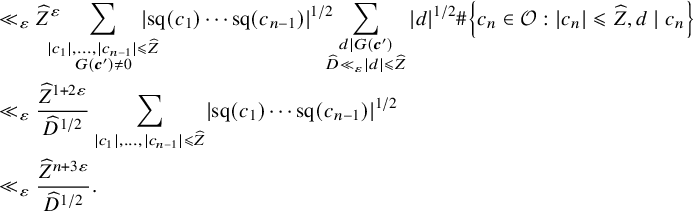
This is satisfactory for the proposition on observing that
$\widehat D\gg \widehat B^{4/n}/\widehat Z^\varepsilon $
 .
.
In order to deal with the remaining contribution from
${\boldsymbol {c}}$
 for which
$G({\boldsymbol {c}}')=0$
for which
$G({\boldsymbol {c}}')=0$
 , we note that for fixed
$c_1,\dots ,c_{n-2}$
, we note that for fixed
$c_1,\dots ,c_{n-2}$
 , there are only finitely many choices of
$c_{n-1}$
, there are only finitely many choices of
$c_{n-1}$
 for which
$G({\boldsymbol {c}}')=0$
for which
$G({\boldsymbol {c}}')=0$
 . This is due to the fact that the coefficient of
$c_{n-1}^{\deg G}$
. This is due to the fact that the coefficient of
$c_{n-1}^{\deg G}$
 appears with a nonzero coefficient, as observed by Heath-Brown [Reference Heath-Brown28, Eq. (4.2)]. Hence we obtain the overall contribution
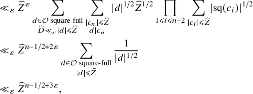
which thereby completes the proof.
7.4 Final touches
We combine Propositions 7.3 and 7.6 in (7.2) to deduce that
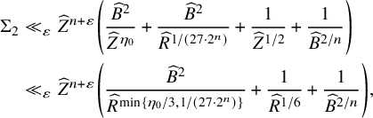
since
$Z\geqslant R/3$
 . The middle term is dominated by the first term. Moreover, we clearly have
$\min \{\eta _0/3,1/(27\cdot 2^{n})\} \geqslant \eta _0/9$
. The middle term is dominated by the first term. Moreover, we clearly have
$\min \{\eta _0/3,1/(27\cdot 2^{n})\} \geqslant \eta _0/9$
 . Balancing for B, we deduce that

where
$ \eta _1= \eta _0/(9n+9). $

We may now deduce the statement of Theorem 7.1, recalling the notation
$\Sigma _A=\Sigma _A(Z,R)$
 for any
$2\leqslant A\leqslant 2+\delta $
for any
$2\leqslant A\leqslant 2+\delta $
 and any
$0\leqslant R\leqslant 3Z$
and any
$0\leqslant R\leqslant 3Z$
 . We claim that

which will clearly suffice for the theorem, in the light of (7.1). If
$Z\leqslant 2R$
 then the statement follows from (7.8), on choosing
$\varepsilon \leqslant \eta _1/4$
then the statement follows from (7.8), on choosing
$\varepsilon \leqslant \eta _1/4$
 . Suppose next that
$Z>2R$
. Suppose next that
$Z>2R$
 and open up the square to get

on noting that
$S^\natural _{r_1}(\boldsymbol {c})S^\natural _{r_2}(\boldsymbol {c})$
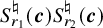 only depends on the value of
${\boldsymbol {c}}$
only depends on the value of
${\boldsymbol {c}}$
 modulo
$r_1r_2$
modulo
$r_1r_2$
 . The inner cardinality is
$O(\widehat Z^n/\widehat R^{2n})$
. The inner cardinality is
$O(\widehat Z^n/\widehat R^{2n})$
 , whence

by Lemma 7.7. The claim now follows on appealing to (7.8).
Lemma 7.7. Suppose
$\lvert \boldsymbol {d} \rvert \leqslant r_1r_2$
 . Then there exists
$\boldsymbol {c}\in \mathcal {S}_2$
. Then there exists
$\boldsymbol {c}\in \mathcal {S}_2$
 with
$\lvert \boldsymbol {c} \rvert \leqslant q^n\, \lvert r_1r_2 \rvert $
with
$\lvert \boldsymbol {c} \rvert \leqslant q^n\, \lvert r_1r_2 \rvert $
 and
$\boldsymbol {c}\equiv \boldsymbol {d}\bmod {r_1r_2}$
and
$\boldsymbol {c}\equiv \boldsymbol {d}\bmod {r_1r_2}$
 .
.
Proof. Let
$H(\boldsymbol {c}) = c_1\cdots c_n F^\ast (\boldsymbol {c})$
 . Let
$S = \{\boldsymbol {d} + r_1r_2\boldsymbol {k}: \lvert \boldsymbol {k} \rvert \leqslant q^n\}$
. Let
$S = \{\boldsymbol {d} + r_1r_2\boldsymbol {k}: \lvert \boldsymbol {k} \rvert \leqslant q^n\}$
 . We want to find
$\boldsymbol {c}\in S$
. We want to find
$\boldsymbol {c}\in S$
 with
$H(\boldsymbol {c})\ne 0$
with
$H(\boldsymbol {c})\ne 0$
 . The set S is a Cartesian product
$\prod _{1\leqslant j\leqslant n} I_j$
. The set S is a Cartesian product
$\prod _{1\leqslant j\leqslant n} I_j$
 , for some sets
$I_1,\dots ,I_n\subseteq \mathcal {O}$
, for some sets
$I_1,\dots ,I_n\subseteq \mathcal {O}$
 of size
$\lvert I_j \rvert = q^{n+1}$
of size
$\lvert I_j \rvert = q^{n+1}$
 . Since
$\deg {H} = n + 3\cdot 2^{n-2} < 2^n + 2^n \leqslant \lvert I_j \rvert $
. Since
$\deg {H} = n + 3\cdot 2^{n-2} < 2^n + 2^n \leqslant \lvert I_j \rvert $
 for all j, the desired
$\boldsymbol {c}$
for all j, the desired
$\boldsymbol {c}$
 exists by the combinatorial nullstellensatz [Reference Alon1, Theorem 1.2] in the field K.
8 Endgame outside dual variety
Let w be as in § 5 with the properties specified in Hypothesis 5.3, but with parameter
$L=0$
 . Let
. Let

where we recall that Q is chosen in such a way that
$|P|^{3/2}\asymp \widehat {Q}$
 . By Lemma 5.1 we have
$I_r(\boldsymbol {c})=0$
. By Lemma 5.1 we have
$I_r(\boldsymbol {c})=0$
 unless
$|\boldsymbol {c}|\ll |r|\text {max}\{1, |P|^3|r|^{-1}\widehat {Q}^{-1}\}|P|^{-1}\ll |P|^{1/2}$
unless
$|\boldsymbol {c}|\ll |r|\text {max}\{1, |P|^3|r|^{-1}\widehat {Q}^{-1}\}|P|^{-1}\ll |P|^{1/2}$
 . In particular, the sum over
$\boldsymbol {c}$
. In particular, the sum over
$\boldsymbol {c}$
 in the definition of
$E_1(P)$
in the definition of
$E_1(P)$
 only runs over vectors
$\boldsymbol {c}\in \mathcal {O}^n$
only runs over vectors
$\boldsymbol {c}\in \mathcal {O}^n$
 with
$|\boldsymbol {c}|\ll |P|^{1/2}$
with
$|\boldsymbol {c}|\ll |P|^{1/2}$
 . Moreover, a simple change of variables shows that Lemma 5.5 implies
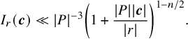
We also keep in mind the
$L=0$
 case of Lemma 5.6, which implies the following:

The primary goal of this section is to establish the following result.
Proposition 8.1. Assume Conjecture 4.5 holds. If
$F=x_1^3+\dots +x_6^3$
 , then
$ E_1(P)\ll |P|^3. $
, then
$ E_1(P)\ll |P|^3. $

We begin by dealing with the contribution from
$c_1\cdots c_n=0$
 , which already follows from [Reference Glas and Hochfilzer26]. Let
$\mathcal {I}\subset \{1,\dots , n\}$
, which already follows from [Reference Glas and Hochfilzer26]. Let
$\mathcal {I}\subset \{1,\dots , n\}$
 with
$\#\mathcal {I}=t$
with
$\#\mathcal {I}=t$
 and define

Let us also fix
$0\leqslant Y\leqslant Q$
 . We will now consider the contribution to
$E_1(P)$
. We will now consider the contribution to
$E_1(P)$
 coming from vectors
$\boldsymbol {c}\in \mathcal {R}(C)$
coming from vectors
$\boldsymbol {c}\in \mathcal {R}(C)$
 and
$r\in \mathcal {O}^+$
and
$r\in \mathcal {O}^+$
 with
$|r|=\widehat {Y}$
with
$|r|=\widehat {Y}$
 . Since the contribution from
$\widehat {C}\gg |P|^{1/2}$
. Since the contribution from
$\widehat {C}\gg |P|^{1/2}$
 vanishes, it is clear that there are at most
$O(\log ^2 |P|)$
vanishes, it is clear that there are at most
$O(\log ^2 |P|)$
 permissible choices for pairs
$(C,Y)$
permissible choices for pairs
$(C,Y)$
 . It follows from the last display on page 21 of [Reference Glas and Hochfilzer26] that

Note that they work with a different weight function; nevertheless, the estimate continues to hold in our setting as we have the stronger integral estimate (8.2) at our disposal. Since we are assuming that
$F^*(\boldsymbol {c})\neq 0$
 and
$c_1\cdots c_n=0$
and
$c_1\cdots c_n=0$
 , we must have
$1\leqslant t \leqslant n-1$
, we must have
$1\leqslant t \leqslant n-1$
 . One now easily sees that the expression above is maximal at
$t=1$
. One now easily sees that the expression above is maximal at
$t=1$
 or
$t=n-1$
or
$t=n-1$
 . The contribution from
$t=n-1$
. The contribution from
$t=n-1$
 is
is

while
$t=1$
 gives
gives

where we used that
$n\geqslant 3$
 and
$\widehat {C}\ll |P|^{1/2}$
and
$\widehat {C}\ll |P|^{1/2}$
 . We have
$3n/4-7/4<n-3$
. We have
$3n/4-7/4<n-3$
 and
$3n/4-13/8<n-3$
and
$3n/4-13/8<n-3$
 for
$n\geqslant 6$
for
$n\geqslant 6$
 and since there are at most
$O(\log ^2 |P|)$
and since there are at most
$O(\log ^2 |P|)$
 choices for
$(Y,C)$
choices for
$(Y,C)$
 , this shows that the contribution from
$c_1\cdots c_n=0$
, this shows that the contribution from
$c_1\cdots c_n=0$
 to
$E_1(P)$
to
$E_1(P)$
 is
$O(|P|^{n-3-\delta })$
is
$O(|P|^{n-3-\delta })$
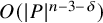 for some
$\delta>0$
for some
$\delta>0$
 . This is satisfactory for Proposition 8.1.
Next, we factor
$r=r_1r_2$
 , where
$r_1\in \mathcal {R}_{\boldsymbol {c}}^{\text {G}}$
, where
$r_1\in \mathcal {R}_{\boldsymbol {c}}^{\text {G}}$
 and
$r_2\in \mathcal {R}_{\boldsymbol {c}}^{\text {B}}$
and
$r_2\in \mathcal {R}_{\boldsymbol {c}}^{\text {B}}$
 . For
$1\leqslant \widehat {C}\ll |P|^{1/2}$
. For
$1\leqslant \widehat {C}\ll |P|^{1/2}$
 and
$0\leqslant Y_1+Y_2\leqslant Q$
and
$0\leqslant Y_1+Y_2\leqslant Q$
 , we shall write
$Y=Y_1+Y_2$
, we shall write
$Y=Y_1+Y_2$
 and consider the sum
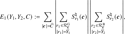
where the sum over
$\boldsymbol {c}$
 runs over
$\boldsymbol {c}\in \mathcal {O}^n$
runs over
$\boldsymbol {c}\in \mathcal {O}^n$
 with
$c_1\cdots c_n\neq 0$
with
$c_1\cdots c_n\neq 0$
 and
$F^*(\boldsymbol {c})\neq 0$
and
$F^*(\boldsymbol {c})\neq 0$
 . We will now provide an upper bound for
$E_1(Y_1,Y_2,C)$
. We will now provide an upper bound for
$E_1(Y_1,Y_2,C)$
 depending on the size of C and the relative size of
$Y_2$
depending on the size of C and the relative size of
$Y_2$
 compared to
$\widehat {Q}/\widehat {Y}$
compared to
$\widehat {Q}/\widehat {Y}$
 . For the rest of this section, let
$\delta>0$
. For the rest of this section, let
$\delta>0$
 be a fixed small real number.
8.1 The case
$\widehat {C}<|P|^{1/2-\delta }$
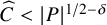
In this case it suffices to use the old estimates from [Reference Glas and Hochfilzer26] and [Reference Browning and Vishe12]. Applying Propositions 6.9 and 6.8 in succession gives

Combining this with (8.2) shows that the contribution to
$E_1(P)$
 with
$\widehat {C}\leqslant |P|^{1/2-\delta }$
with
$\widehat {C}\leqslant |P|^{1/2-\delta }$
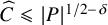 is at most

where we used that
$\widehat {C}\ll |P|^{1/2-\delta }$
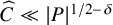 ,
$\widehat {Y}\ll |P|^{3/2}$
,
$\widehat {Y}\ll |P|^{3/2}$
 and that the number of available
$(Y_1,Y_2,C)$
and that the number of available
$(Y_1,Y_2,C)$
 is
$O(\log |P|)=O(|P|^{\varepsilon })$
is
$O(\log |P|)=O(|P|^{\varepsilon })$
 . Thus the contribution to
$E_1(P)$
. Thus the contribution to
$E_1(P)$
 is at most
$O(|P|^{n-3})$
is at most
$O(|P|^{n-3})$
 for
$n\geqslant 6$
for
$n\geqslant 6$
 , which is satisfactory.
8.2 The case
$\widehat {C}\geqslant |P|^{1/2-\delta }$
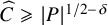
We shall divide the complementary case into two further subcases. First, let from now on
$\varepsilon>0$
 be a fixed, sufficiently small real number. We then define
$\alpha = (1/2-\varepsilon )/\deg F^*$
be a fixed, sufficiently small real number. We then define
$\alpha = (1/2-\varepsilon )/\deg F^*$
 and
and

The case
$\widehat {Y}_2^{n+\varepsilon }\leqslant \widehat {W}^{\alpha /2}$
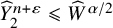
In this regime we require the full strength of Conjecture 4.5 and of Lemma 5.8. To make use of Lemma 5.8, we need the following auxiliary result.
Lemma 8.2. Let
$G\in \mathcal {O}[c_1,\dots , c_n]$
 be a polynomial. Let
$C\geqslant 0$
be a polynomial. Let
$C\geqslant 0$
 and
$\lambda \in \mathbb {R}$
and
$\lambda \in \mathbb {R}$
 . Then

Proof. By Lemma 2.7, we may assume
$\deg _{c_1}(G) = \deg {G}$
 . By the
$v=\infty $
. By the
$v=\infty $
 case of (2.20), the number of available choices for
$c_1$
case of (2.20), the number of available choices for
$c_1$
 is
$\ll _G 1 + \widehat C \widehat \lambda ^{1/\deg G}$
is
$\ll _G 1 + \widehat C \widehat \lambda ^{1/\deg G}$
 , once
$c_2,\dots ,c_n$
, once
$c_2,\dots ,c_n$
 are specified. Summing over
$c_2,\dots ,c_n$
are specified. Summing over
$c_2,\dots ,c_n$
 , the cardinality in Lemma 8.2 is

(A referee pointed out to us that the middle bound
$\widehat {C}^n (\widehat \lambda +\widehat {C}^{-\deg G})^{1/\deg G}$
 might be useful for simplifying some of the subsequent estimates of § 8, as well as the choice of
$\widehat W$
might be useful for simplifying some of the subsequent estimates of § 8, as well as the choice of
$\widehat W$
 in (8.3). However, in order to maintain compatibility with the published sequel [Reference Browning, Glas and Wang8], we do not explore such improvements in the present paper.)
Recall from Lemma 5.8 that
$I_r(\boldsymbol {c})=0$
 unless
$|F^*(P\boldsymbol {c}/r)|\ll 1 + (|P||\boldsymbol {c}|/\widehat {Y})^{\deg F*-1}$
unless
$|F^*(P\boldsymbol {c}/r)|\ll 1 + (|P||\boldsymbol {c}|/\widehat {Y})^{\deg F*-1}$
 . After setting

it then follows from Hölder’s inequality with
$p_1=2-\varepsilon _0$
 ,
$p_2=(2-\varepsilon _0)/(1-2\varepsilon _0)$
,
$p_2=(2-\varepsilon _0)/(1-2\varepsilon _0)$
 and
$p_3=(2-\varepsilon _0)/\varepsilon _0$
and
$p_3=(2-\varepsilon _0)/\varepsilon _0$
 that
that

We can now apply the trivial estimate
$|S_{r_2}^\natural (\boldsymbol {c})|\leqslant |r_2|^{(n+1)/2}$
 and invoke Lemma 2.3 to estimate the sum over
$r_2$
and invoke Lemma 2.3 to estimate the sum over
$r_2$
 . Combining this with Conjecture 4.5 with
$Z=\lceil \text {max}(C,\frac 13Y_1) \rceil $
. Combining this with Conjecture 4.5 with
$Z=\lceil \text {max}(C,\frac 13Y_1) \rceil $
 and
$R=Y_1$
and
$R=Y_1$
 to estimate the sum over
$r_1$
to estimate the sum over
$r_1$
 , we get

where
$\varepsilon := \frac 12 - (1-2\varepsilon _0)/(2-\varepsilon _0) = \frac 34\varepsilon _0 + O(\varepsilon _0^2)$
 . Note that Lemma 8.2 implies that

Together with the last display and (8.2) this shows that the contribution to
$E_1(P)$
 from those
$(Y_1,Y_2, C)$
from those
$(Y_1,Y_2, C)$
 under consideration is
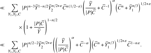
One can check that
$-\alpha +n(1/2+\varepsilon )+1-n\varepsilon>0$
 and
$-\alpha +1-n\varepsilon>0$
and
$-\alpha +1-n\varepsilon>0$
 , so that upon recalling
$\widehat {C}\ll |P|^{1/2}$
, so that upon recalling
$\widehat {C}\ll |P|^{1/2}$
 , we get that the contribution is
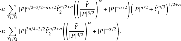
We can now use that

which together with the definition of
$\widehat {W}$
 in (8.3) implies that the contribution is
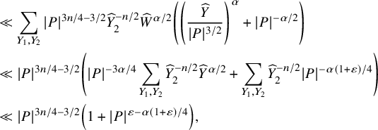
where we used that
$\sum _{Y_1,Y_2}\widehat {Y}_2^{-n/2}\widehat {Y}^{\alpha /2}\ll |P|^{3\alpha /4}$
 , because
$\widehat {Y}\ll |P|^{3/2}$
, because
$\widehat {Y}\ll |P|^{3/2}$
 . Therefore, as
$\varepsilon (1-\alpha /4)-\alpha <0$
. Therefore, as
$\varepsilon (1-\alpha /4)-\alpha <0$
 for
$\varepsilon $
for
$\varepsilon $
 sufficiently small, the contribution from the case under consideration is again
$O(|P|^{n-3})$
sufficiently small, the contribution from the case under consideration is again
$O(|P|^{n-3})$
 for
$n\geqslant 6$
for
$n\geqslant 6$
 .
.
The case
$\widehat {Y}_2^{n+\varepsilon }>\widehat {W}^{\alpha /2}$
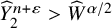
Applying Hölder’s inequality to
$E_1(Y_1,Y_2,C)$
 with
$p_1=2-\varepsilon $
with
$p_1=2-\varepsilon $
 and
$p_2=(2-\varepsilon )/(1-\varepsilon )$
and
$p_2=(2-\varepsilon )/(1-\varepsilon )$
 gives
gives

Next we use Conjecture 4.5 with
$Z=\lceil \text {max}(C,\frac 13Y_1) \rceil $
 and
$R=Y_1$
and
$R=Y_1$
 to estimate the first sum and Theorem 7.1 with
$Z=\lceil \text {max}(C,\frac 13Y_2) \rceil $
to estimate the first sum and Theorem 7.1 with
$Z=\lceil \text {max}(C,\frac 13Y_2) \rceil $
 and
$R=Y_2$
and
$R=Y_2$
 for the second, to obtain

for some
$\eta>0$
 . If we choose
$\delta $
. If we choose
$\delta $
 sufficiently small, we have
$\widehat {C}>|P|^{1/2-\delta }\gg |P|^{1/4}\gg \widehat {Y}^{1/6}$
sufficiently small, we have
$\widehat {C}>|P|^{1/2-\delta }\gg |P|^{1/4}\gg \widehat {Y}^{1/6}$
 . As
$\widehat {Y}_1\widehat {Y}_2=\widehat {Y}$
. As
$\widehat {Y}_1\widehat {Y}_2=\widehat {Y}$
 , this implies that
$\widehat {Y}_1^{1/3}\ll \widehat {C}$
, this implies that
$\widehat {Y}_1^{1/3}\ll \widehat {C}$
 or
$\widehat {Y}_2^{1/3}\ll \widehat {C}$
or
$\widehat {Y}_2^{1/3}\ll \widehat {C}$
 . Therefore, the bound in (8.4) gives

Moreover, if the third term in the brackets dominates then we must have
$\widehat {C}^3\ll \widehat {Y}_2$
 . Thus, on noting that
$1/p_1-1/p_2>0$
. Thus, on noting that
$1/p_1-1/p_2>0$
 , we obtain

where we trivially estimated
$\widehat {Y}_1,\widehat {Y}_2\leqslant \widehat {Y}$
 . Moreover, we have set
$\eta '=\eta /p_2$
. Moreover, we have set
$\eta '=\eta /p_2$
 , which satisfies
$\eta '\geqslant \eta /4$
, which satisfies
$\eta '\geqslant \eta /4$
 for
$\varepsilon $
for
$\varepsilon $
 small enough.
Observe that
$n/p_2+1-n/2>0$
 , so that summing over
$Y_1,Y_2,C$
, so that summing over
$Y_1,Y_2,C$
 and using the integral estimate (8.2) shows that the contribution from this case to
$E_1(P)$
and using the integral estimate (8.2) shows that the contribution from this case to
$E_1(P)$
 is
is
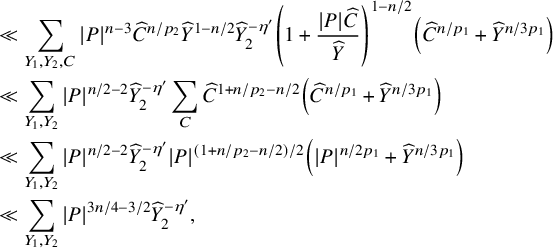
where we used
$1/p_1+1/p_2=1$
 and that
$\widehat {C}\ll |P|^{1/2}$
and that
$\widehat {C}\ll |P|^{1/2}$
 , as well as the fact that
$\widehat {Y}\ll |P|^{3/2}$
, as well as the fact that
$\widehat {Y}\ll |P|^{3/2}$
 . Since
$3n/4-3/2\leqslant n-3$
. Since
$3n/4-3/2\leqslant n-3$
 for
$n\geqslant 6$
for
$n\geqslant 6$
 , to complete our treatment of
$E_1(P)$
, to complete our treatment of
$E_1(P)$
 it will suffice to show that
$\sum _{Y_1,Y_2}\widehat {Y}_2^{-\eta '}\ll 1$
it will suffice to show that
$\sum _{Y_1,Y_2}\widehat {Y}_2^{-\eta '}\ll 1$
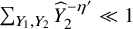 . To do so, recall that
$\widehat {Y}_2^{n+\varepsilon }> \widehat {W}^{\alpha /2}$
. To do so, recall that
$\widehat {Y}_2^{n+\varepsilon }> \widehat {W}^{\alpha /2}$
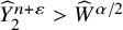 . If we set
$\beta = \eta '\alpha /(4(n+\varepsilon ))$
. If we set
$\beta = \eta '\alpha /(4(n+\varepsilon ))$
 , then recalling the definition of
$\widehat {W}$
, then recalling the definition of
$\widehat {W}$
 in (8.3) this implies
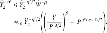
Therefore, as
$\sum _{Y_1,Y_2} |P|^{\beta (\varepsilon -1)/2} \leqslant Q^2 |P|^{\beta (\varepsilon -1)/2}\ll 1$
 , we get
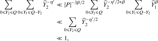
as
$\eta '>0$
 . This completes our proof of Proposition 8.1.
9 Contribution from the centre
In this section we estimate the contribution from
$\boldsymbol {c}=\mathbf {0}$
 in (2.9). This takes the shape
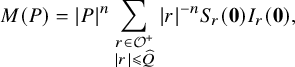
where
$S_r(\boldsymbol {0})$
 is given by (2.6), and
$I_r(\boldsymbol {0})$
is given by (2.6), and
$I_r(\boldsymbol {0})$
 is given by (2.7) and (2.8). The following is the main goal of this section.
Proposition 9.1. Let
$n\geqslant 5$
 . Then
$ M(P)\ll |P|^{n-3}, $
. Then
$ M(P)\ll |P|^{n-3}, $
 for any
$Q\geqslant 0$
for any
$Q\geqslant 0$
 .
.
To begin with, it follows from (8.2) that
$ I_r(\mathbf 0) \ll |P|^{-3}, $
 if
$n\geqslant 3$
if
$n\geqslant 3$
 . Hence

if
$n\geqslant 3$
 . We shall require the following technical result, which will also be useful in the next section.
Lemma 9.2. If
$R\geqslant 0$
 and
$\varepsilon>0$
and
$\varepsilon>0$
 , then

The statement of Proposition 9.1 follows on combining this result with (9.2) to deduce that
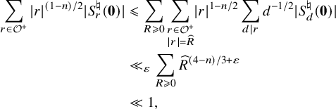
if
$n\geqslant 5$
 .
.
Proof of Lemma 9.2
Recalling the notation for
$\operatorname {\mathrm {cub}}(d)$
 introduced in (6.1), it follows from Lemma 6.3 that
$|d|^{-1/2}S_{d}^\natural (\boldsymbol {0})\ll _\varepsilon |\operatorname {\mathrm {cub}}(d)|^{n/6+\varepsilon }$
introduced in (6.1), it follows from Lemma 6.3 that
$|d|^{-1/2}S_{d}^\natural (\boldsymbol {0})\ll _\varepsilon |\operatorname {\mathrm {cub}}(d)|^{n/6+\varepsilon }$
 , for any
$\varepsilon>0$
, for any
$\varepsilon>0$
 . Hence

on taking the trivial estimate for the divisor function. Writing
$r=r_1r_2$
 , where
$r_1$
, where
$r_1$
 is cube-free and
$r_2$
is cube-free and
$r_2$
 is cube-full, we see that
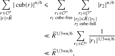
since
$n\geqslant 5$
 . The statement of the lemma easily follows.
10 Contribution from dual variety
Let w be as in § 5, with the properties specified in Hypothesis 5.3, with parameter
$L=0$
 . The purpose of this section is to study the quantity

where Q is chosen so that
$|P|^{3/2}\asymp \widehat {Q}$
 and
$I_r(\boldsymbol {c})=0$
and
$I_r(\boldsymbol {c})=0$
 unless
$|\boldsymbol {c}|\ll |P|^{1/2}$
unless
$|\boldsymbol {c}|\ll |P|^{1/2}$
 , by Lemma 5.1. We shall be interested in this quantity when
$n=6$
, by Lemma 5.1. We shall be interested in this quantity when
$n=6$
 and
$F=x_1^3+\dots +x_6^3$
and
$F=x_1^3+\dots +x_6^3$
 . Let
$V\subset \mathbb {P}_K^5$
. Let
$V\subset \mathbb {P}_K^5$
 denote the cubic hypersurface defined by F.
Let
$\Upsilon $
 be the set of
$3$
be the set of
$3$
 -dimensional K-vector spaces
$L\subseteq K^6$
-dimensional K-vector spaces
$L\subseteq K^6$
 with
$F\vert _L = 0$
with
$F\vert _L = 0$
 . (Note that the projectivisation of
$\Upsilon $
. (Note that the projectivisation of
$\Upsilon $
 is the K-point set of the Fano variety
$F_2(V)$
is the K-point set of the Fano variety
$F_2(V)$
 of planes on V.) Since F is nonsingular, it is well-known that
$\Upsilon $
of planes on V.) Since F is nonsingular, it is well-known that
$\Upsilon $
 is finite, as explained by Starr [Reference Browning and Heath-Brown9, Appendix]. The task of estimating
$E_2(P)$
is finite, as explained by Starr [Reference Browning and Heath-Brown9, Appendix]. The task of estimating
$E_2(P)$
 is divided into two steps. First, in Proposition 10.6 we will establish a bias in the exponential sum
$S_r(\boldsymbol {c})$
is divided into two steps. First, in Proposition 10.6 we will establish a bias in the exponential sum
$S_r(\boldsymbol {c})$
 whenever
$\boldsymbol {c}\in L^\perp $
whenever
$\boldsymbol {c}\in L^\perp $
 , for some
$L\in \Upsilon $
, for some
$L\in \Upsilon $
 . Note that the projectivisation of
$L^\perp $
. Note that the projectivisation of
$L^\perp $
 corresponds to a plane contained in the dual variety of V. Planes contained in the dual variety of V correspond to planes in V via bi-duality. Using Poisson summation, we shall show that the bias of the exponential sums gives a contribution that exactly matches the contribution from the points of bounded height on
$\bigcup _{L\in \Upsilon } L$
corresponds to a plane contained in the dual variety of V. Planes contained in the dual variety of V correspond to planes in V via bi-duality. Using Poisson summation, we shall show that the bias of the exponential sums gives a contribution that exactly matches the contribution from the points of bounded height on
$\bigcup _{L\in \Upsilon } L$
 . The second task will be to show that the vectors
$\boldsymbol {c}\in \mathcal {O}^6$
. The second task will be to show that the vectors
$\boldsymbol {c}\in \mathcal {O}^6$
 such that
$F^*(\boldsymbol {c})= 0$
such that
$F^*(\boldsymbol {c})= 0$
 , but which do not lie on
$L^\perp $
, but which do not lie on
$L^\perp $
 for any
$L\in \Upsilon $
for any
$L\in \Upsilon $
 , are sparse and form a negligible contribution.
The goal of this section is summarised in the following result.
Proposition 10.1. Let
$\varepsilon>0$
 . If
$F=x_1^3+\dots +x_6^3$
. If
$F=x_1^3+\dots +x_6^3$
 , then

In fact, much of our argument carries over to general F in
$n\in \{4,6\}$
 variables, but a restriction to diagonal F is necessary when it comes to handling square-full moduli. Throughout this section we shall therefore assume that
$F=x_1^3+\dots +x_6^3$
variables, but a restriction to diagonal F is necessary when it comes to handling square-full moduli. Throughout this section we shall therefore assume that
$F=x_1^3+\dots +x_6^3$
 , unless otherwise indicated. For later convenience, we note that if
$\operatorname {\mathrm {char}}(\mathbb {F}_q)> 3$
, unless otherwise indicated. For later convenience, we note that if
$\operatorname {\mathrm {char}}(\mathbb {F}_q)> 3$
 there is a unique
$L\in \Upsilon $
there is a unique
$L\in \Upsilon $
 up to an
$\mathbb {F}_q$
up to an
$\mathbb {F}_q$
 -linear automorphism of F, given by

A proof of this fact is given in [Reference Wang52, Remark 6.3.8], based on [Reference Kontogeorgis39,Reference Shioda49].
10.1 Geometric preliminaries
Throughout this subsection, k denotes an arbitrary field with
$\operatorname {\mathrm {char}}(k)\neq 2$
 and we shall adopt the notation
$\mathbb {P}(E)$
and we shall adopt the notation
$\mathbb {P}(E)$
 for the projectivisation of a k-vector space E. (In particular,
$\mathbb {P}^n$
for the projectivisation of a k-vector space E. (In particular,
$\mathbb {P}^n$
 denotes the projective space
$\mathbb {P}(k^{n+1})$
denotes the projective space
$\mathbb {P}(k^{n+1})$
 .) Suppose that
$V\subset \mathbb {P}^5$
.) Suppose that
$V\subset \mathbb {P}^5$
 is a smooth cubic fourfold containing a k-plane
$M\subset \mathbb {P}^5$
is a smooth cubic fourfold containing a k-plane
$M\subset \mathbb {P}^5$
 , corresponding to a three-dimensional vector space
$L\subset k^6$
, corresponding to a three-dimensional vector space
$L\subset k^6$
 . Projection away from M, defined by the natural map
$\mathbb {P}(k^6)\to \mathbb {P}(k^6/L)$
. Projection away from M, defined by the natural map
$\mathbb {P}(k^6)\to \mathbb {P}(k^6/L)$
 , gives a morphism
$V\setminus M \to \mathbb {P}(k^6/L)$
, gives a morphism
$V\setminus M \to \mathbb {P}(k^6/L)$
 . Blowing up V along M resolves the indeterminacy locus and gives a fibration
$\widetilde {V}\to \mathbb {P}(k^6/L)$
. Blowing up V along M resolves the indeterminacy locus and gives a fibration
$\widetilde {V}\to \mathbb {P}(k^6/L)$
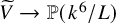 whose fibres are projective quadric surfaces. Being the blow-up of a smooth variety along a smooth subvariety,
$\widetilde {V}$
whose fibres are projective quadric surfaces. Being the blow-up of a smooth variety along a smooth subvariety,
$\widetilde {V}$
 is also smooth. If we denote by
$\mathcal {C}\subset \mathbb {P}(k^6/L)$
is also smooth. If we denote by
$\mathcal {C}\subset \mathbb {P}(k^6/L)$
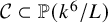 the zero scheme of the determinant of the matrices that define the quadratic forms in the fibres, it follows from Proposition 1.2 and Exemple 1.4.2 of Beauville [Reference Beauville4] that
$\mathcal {C}$
the zero scheme of the determinant of the matrices that define the quadratic forms in the fibres, it follows from Proposition 1.2 and Exemple 1.4.2 of Beauville [Reference Beauville4] that
$\mathcal {C}$
 is a curve of degree 6 which is either smooth or has ordinary double points. Let
$L^\perp $
is a curve of degree 6 which is either smooth or has ordinary double points. Let
$L^\perp $
 be the orthogonal complement of L inside
$k^6$
be the orthogonal complement of L inside
$k^6$
 and note that
$\mathbb {P}(L^\perp )$
and note that
$\mathbb {P}(L^\perp )$
 parameterises hyperplanes in
$\mathbb {P}(k^6)$
parameterises hyperplanes in
$\mathbb {P}(k^6)$
 containing M. If
$\boldsymbol {c}\in \mathbb {P}(L^\perp )$
containing M. If
$\boldsymbol {c}\in \mathbb {P}(L^\perp )$
 , we shall write
$H_{\boldsymbol {c}}$
, we shall write
$H_{\boldsymbol {c}}$
 for the corresponding hyperplane containing M in
$\mathbb {P}(k^6)$
for the corresponding hyperplane containing M in
$\mathbb {P}(k^6)$
 and
$H_{\boldsymbol {c}}'$
and
$H_{\boldsymbol {c}}'$
 for the image of
$H_{\boldsymbol {c}}$
for the image of
$H_{\boldsymbol {c}}$
 in
$\mathbb {P}(k^6/L)$
in
$\mathbb {P}(k^6/L)$
 , which defines a projective line.
If we denote by
$V_{\boldsymbol {c}}=H_{\boldsymbol {c}}\cap V$
 , then we get again a morphism
$V_{\boldsymbol {c}}\setminus M\to H_{\boldsymbol {c}}'$
, then we get again a morphism
$V_{\boldsymbol {c}}\setminus M\to H_{\boldsymbol {c}}'$
 by projecting away from M. Blowing up
$V_{\boldsymbol {c}}$
by projecting away from M. Blowing up
$V_{\boldsymbol {c}}$
 gives a fibration
$\widetilde {V}_{\boldsymbol {c}}\to H_{\boldsymbol {c}}'$
gives a fibration
$\widetilde {V}_{\boldsymbol {c}}\to H_{\boldsymbol {c}}'$
 into quadric surfaces and the locus of degenerate quadric surfaces is given by
$\mathcal {C}_{\boldsymbol {c}}=H_{\boldsymbol {c}}'\cap \mathcal {C}$
into quadric surfaces and the locus of degenerate quadric surfaces is given by
$\mathcal {C}_{\boldsymbol {c}}=H_{\boldsymbol {c}}'\cap \mathcal {C}$
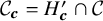 .
.
Note that after a suitable change of variables we may assume that L is given by
$x_1=x_2=x_3=0$
 , so that V is defined by a cubic form of the shape

for some quadratic forms
$Q_1, Q_2, Q_3 \in k[x_1,x_2,x_3,y_1,y_2,y_3]$
 . Upon defining

we obtain a conic bundle
$W\to \mathbb {P}^2$
 by projecting to the first factor. A straightforward computation with the Jacobian criterion shows that smoothness of V along L implies smoothness of W. Hence, on appealing once again to Proposition 1.2 of Beauville [Reference Beauville4], it follows that
$f(\boldsymbol {s})=\det (s_1M_1+s_2M_2+s_3M_3)$
by projecting to the first factor. A straightforward computation with the Jacobian criterion shows that smoothness of V along L implies smoothness of W. Hence, on appealing once again to Proposition 1.2 of Beauville [Reference Beauville4], it follows that
$f(\boldsymbol {s})=\det (s_1M_1+s_2M_2+s_3M_3)$
 is nonzero as a polynomial in
$\boldsymbol {s}$
is nonzero as a polynomial in
$\boldsymbol {s}$
 , where
$M_i$
, where
$M_i$
 is the
$3\times 3$
is the
$3\times 3$
 matrix underlying
$Q_i$
matrix underlying
$Q_i$
 . The equation
$f=0$
. The equation
$f=0$
 thus defines a curve
$\mathcal {D}\subset \mathbb {P}^2$
thus defines a curve
$\mathcal {D}\subset \mathbb {P}^2$
 .
.
Definition 10.2. Let
$\boldsymbol {c}\in L^\perp \setminus \{\boldsymbol {0}\}$
 . We say that
$\boldsymbol {c}$
. We say that
$\boldsymbol {c}$
 is good if
-
(i) $\mathcal {C}_{\boldsymbol {c}}$
is smooth of dimension
$0$
, -
(ii) $H_{\boldsymbol {c}}\subset \mathbb {P}^5$
contains no plane contained in V other than M, -
(iii) $H^{\prime }_{\boldsymbol {c}}$
is not an irreducible component of
$\mathcal {D}$
,


and we say that
$\boldsymbol {c}$
 is bad otherwise.
Note that the definition depends on the choice of L. The significance of this definition is that hyperplane sections coming from good
$\boldsymbol {c}$
 ’s enjoy good geometric properties and bad vectors
$\boldsymbol {c}$
’s enjoy good geometric properties and bad vectors
$\boldsymbol {c}$
 only occur rarely, as we will see in the next two results.
Lemma 10.3. Suppose
$\boldsymbol {c}$
 is bad. Then
$\boldsymbol {c}$
is bad. Then
$\boldsymbol {c}$
 lies in a subvariety of
$\mathbb {P}(L^\perp )$
lies in a subvariety of
$\mathbb {P}(L^\perp )$
 , all of whose irreducible components have dimension at most one.
Proof. Since
$\mathcal {C}$
 is reduced and has at worst ordinary double points, a generic hyperplane section is smooth of dimension
$0$
is reduced and has at worst ordinary double points, a generic hyperplane section is smooth of dimension
$0$
 . Indeed, as long as
$H^{\prime }_{\boldsymbol {c}}$
. Indeed, as long as
$H^{\prime }_{\boldsymbol {c}}$
 does not lie on the dual variety of
$\mathcal {C}$
does not lie on the dual variety of
$\mathcal {C}$
 or contain one of the singular points of
$\mathcal {C}$
or contain one of the singular points of
$\mathcal {C}$
 , the intersection
$H^{\prime }_{\boldsymbol {c}}\cap \mathcal {C}$
, the intersection
$H^{\prime }_{\boldsymbol {c}}\cap \mathcal {C}$
 will be smooth. Moreover, it will be
$0$
will be smooth. Moreover, it will be
$0$
 -dimensional as long as
$H^{\prime }_{\boldsymbol {c}}$
-dimensional as long as
$H^{\prime }_{\boldsymbol {c}}$
 is not a component of
$\mathcal {C}$
is not a component of
$\mathcal {C}$
 . Each case forces
$\boldsymbol {c}$
. Each case forces
$\boldsymbol {c}$
 to lie on a subvariety of dimension at most one. If
$H_{\boldsymbol {c}}$
to lie on a subvariety of dimension at most one. If
$H_{\boldsymbol {c}}$
 contains two distinct planes contained in V, then it must also contain the linear space they span, which has dimension at least 3. Hyperplanes in
$\mathbb {P}(k^6)$
contains two distinct planes contained in V, then it must also contain the linear space they span, which has dimension at least 3. Hyperplanes in
$\mathbb {P}(k^6)$
 containing a fixed three-dimensional linear space are parameterised by a
$\mathbb {P}^1$
containing a fixed three-dimensional linear space are parameterised by a
$\mathbb {P}^1$
 and since there are only finitely many planes contained in V, this shows that
$\boldsymbol {c}$
and since there are only finitely many planes contained in V, this shows that
$\boldsymbol {c}$
 lies on a union of finitely many lines. Finally, the curve
$\mathcal {D}$
lies on a union of finitely many lines. Finally, the curve
$\mathcal {D}$
 has at most 3 irreducible components and so there are at most 3 possibilities for
$\boldsymbol {c}$
has at most 3 irreducible components and so there are at most 3 possibilities for
$\boldsymbol {c}$
 such that
$H_{\boldsymbol {c}}'$
such that
$H_{\boldsymbol {c}}'$
 is an irreducible component of
$\mathcal {D}$
is an irreducible component of
$\mathcal {D}$
 .
.
Lemma 10.4. Suppose that
$\boldsymbol {c}$
 is good. Then every fibre of the quadric surface bundle
$\widetilde {V}_{\boldsymbol {c}}\to H_{\boldsymbol {c}}'$
is good. Then every fibre of the quadric surface bundle
$\widetilde {V}_{\boldsymbol {c}}\to H_{\boldsymbol {c}}'$
 has at worst isolated singularities.
Proof. For
$\boldsymbol {s}\in H_{\boldsymbol {c}}'$
 , let
$Q_{\boldsymbol {s}}$
, let
$Q_{\boldsymbol {s}}$
 be the fibre above
$\boldsymbol {s}$
be the fibre above
$\boldsymbol {s}$
 in
$\widetilde {V}_{\boldsymbol {c}}$
in
$\widetilde {V}_{\boldsymbol {c}}$
 , which is a projective quadric surface and hence corresponds to some matrix
$M_{\boldsymbol {s}}\in \mathrm {Mat}_{4\times 4}(k)$
, which is a projective quadric surface and hence corresponds to some matrix
$M_{\boldsymbol {s}}\in \mathrm {Mat}_{4\times 4}(k)$
 . The claim of the lemma is now equivalent to
$M_{\boldsymbol {s}}$
. The claim of the lemma is now equivalent to
$M_{\boldsymbol {s}}$
 having rank at least 3. Note that if
$\operatorname {\mathrm {rank}} M_{\boldsymbol {s}} = 1$
having rank at least 3. Note that if
$\operatorname {\mathrm {rank}} M_{\boldsymbol {s}} = 1$
 , then
$Q_{\boldsymbol {s}}$
, then
$Q_{\boldsymbol {s}}$
 contains a double plane. However,
$Q_{\boldsymbol {s}}$
contains a double plane. However,
$Q_{\boldsymbol {s}}$
 is also a fibre of the fibration
$\widetilde {V}\to \mathbb {P}(k^6/L)$
is also a fibre of the fibration
$\widetilde {V}\to \mathbb {P}(k^6/L)$
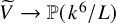 and is thus the residual intersection of a linear
$3$
and is thus the residual intersection of a linear
$3$
 -space containing M with the cubic hypersurface V. Therefore, a result of Zak [Reference Hooley31, Katz’s Appendix, Theorem 2] shows that the singular locus of
$Q_{\boldsymbol {s}}$
-space containing M with the cubic hypersurface V. Therefore, a result of Zak [Reference Hooley31, Katz’s Appendix, Theorem 2] shows that the singular locus of
$Q_{\boldsymbol {s}}$
 has dimension at most 1 and so
$Q_{\boldsymbol {s}}$
has dimension at most 1 and so
$Q_{\boldsymbol {s}}$
 cannot be a double plane. Now assume that
$\operatorname {\mathrm {rank}} M_{\boldsymbol {s}}=2$
cannot be a double plane. Now assume that
$\operatorname {\mathrm {rank}} M_{\boldsymbol {s}}=2$
 . This implies that
$Q_{\boldsymbol {s}}$
. This implies that
$Q_{\boldsymbol {s}}$
 is a union of two distinct planes. However, this is impossible as at least one such plane would be distinct from M and contained in
$H_{\boldsymbol {c}}$
is a union of two distinct planes. However, this is impossible as at least one such plane would be distinct from M and contained in
$H_{\boldsymbol {c}}$
 . This would contradict the assumption that
$\boldsymbol {c}$
. This would contradict the assumption that
$\boldsymbol {c}$
 is good.
10.2 Exponential sums
In this section it is no harder to work with an arbitrary cubic form
$F\in \mathcal {O}[x_1,\dots , x_6]$
 defining a smooth hypersurface
$\mathcal {V}\subset \mathbb {P}^5_{\mathcal {O}}$
defining a smooth hypersurface
$\mathcal {V}\subset \mathbb {P}^5_{\mathcal {O}}$
 . Let
$V:= \mathcal {V}\times \operatorname {\mathrm {Spec}} \mathbb {F}_q(t)$
. Let
$V:= \mathcal {V}\times \operatorname {\mathrm {Spec}} \mathbb {F}_q(t)$
 and for a prime
$\varpi $
and for a prime
$\varpi $
 of
$\mathcal {O}$
of
$\mathcal {O}$
 we let
$\mathbb {F}_\varpi = \mathcal {O}/\varpi \mathcal {O}$
we let
$\mathbb {F}_\varpi = \mathcal {O}/\varpi \mathcal {O}$
 and set
$\mathcal {V}_\varpi := \mathcal {V}\times \operatorname {\mathrm {Spec}} \mathbb {F}_\varpi $
and set
$\mathcal {V}_\varpi := \mathcal {V}\times \operatorname {\mathrm {Spec}} \mathbb {F}_\varpi $
 . Moreover, we fix a K-vector space
$L\subset K^6$
. Moreover, we fix a K-vector space
$L\subset K^6$
 such that
$F_{|L}\equiv 0$
such that
$F_{|L}\equiv 0$
 and denote by
$L^\perp $
and denote by
$L^\perp $
 its orthogonal complement inside
$K^6$
its orthogonal complement inside
$K^6$
 . We then set
$\Lambda = L\cap \mathcal {O}^6$
. We then set
$\Lambda = L\cap \mathcal {O}^6$
 and
$\Lambda ^\perp = L^\perp \cap \mathcal {O}^6$
and
$\Lambda ^\perp = L^\perp \cap \mathcal {O}^6$
 . We shall write M for the subspace of
$\mathbb {P}^{5}$
. We shall write M for the subspace of
$\mathbb {P}^{5}$
 corresponding to L. In addition, we let
$L_\varpi = \Lambda /\varpi \Lambda $
corresponding to L. In addition, we let
$L_\varpi = \Lambda /\varpi \Lambda $
 and
$L^\perp _\varpi = \Lambda ^\perp /\varpi \Lambda ^\perp $
and
$L^\perp _\varpi = \Lambda ^\perp /\varpi \Lambda ^\perp $
 , which are both
$\mathbb {F}_\varpi $
, which are both
$\mathbb {F}_\varpi $
 -vector spaces of dimension 3.
Let
$\boldsymbol {c}\in L^\perp \setminus \{\boldsymbol {0}\}$
 . Abusing the definition of the previous subsection slightly, we shall also say that
$\boldsymbol {c}$
. Abusing the definition of the previous subsection slightly, we shall also say that
$\boldsymbol {c}$
 is good if the corresponding point in projective space is good. Let
$g\in \mathcal {O}[y_1,y_2,y_3]$
is good if the corresponding point in projective space is good. Let
$g\in \mathcal {O}[y_1,y_2,y_3]$
 be a degree 6 form defining the curve
$\mathcal {C}$
be a degree 6 form defining the curve
$\mathcal {C}$
 in
$\mathbb {P}(K^6/L)$
in
$\mathbb {P}(K^6/L)$
 . Note that if
$\boldsymbol {c}\in L^\perp \setminus \{\boldsymbol {0}\}$
. Note that if
$\boldsymbol {c}\in L^\perp \setminus \{\boldsymbol {0}\}$
 is good, then by definition
$\mathcal {C}_{\boldsymbol {c}}\subset H_{\boldsymbol {c}}'$
is good, then by definition
$\mathcal {C}_{\boldsymbol {c}}\subset H_{\boldsymbol {c}}'$
 is smooth. In particular, if we work with coordinates
$(s:t)$
is smooth. In particular, if we work with coordinates
$(s:t)$
 on
$H_{\boldsymbol {c}}'$
on
$H_{\boldsymbol {c}}'$
 , then there exists a separable binary form
$g_{\boldsymbol {c}}\in \mathcal {O}[s,t]$
, then there exists a separable binary form
$g_{\boldsymbol {c}}\in \mathcal {O}[s,t]$
 of degree 6 whose coefficients are degree 6 polynomials in
$\boldsymbol {c}$
of degree 6 whose coefficients are degree 6 polynomials in
$\boldsymbol {c}$
 that define
$\mathcal {C}_{\boldsymbol {c}}$
that define
$\mathcal {C}_{\boldsymbol {c}}$
 .
.
Example 10.5. Suppose that
$L=\{x_1=x_2=x_3=0\}$
 . Then any
$\boldsymbol {c}\in L^\perp \setminus \{\boldsymbol {0}\}$
. Then any
$\boldsymbol {c}\in L^\perp \setminus \{\boldsymbol {0}\}$
 takes the shape
$(c_1,c_2,c_3,0,0,0)$
takes the shape
$(c_1,c_2,c_3,0,0,0)$
 and, without loss of generality, we may assume that
$c_3\neq 0$
and, without loss of generality, we may assume that
$c_3\neq 0$
 and
$c_1,c_2,c_3\in \mathcal {O}$
and
$c_1,c_2,c_3\in \mathcal {O}$
 . Rational points on
$H_{\boldsymbol {c}}'$
. Rational points on
$H_{\boldsymbol {c}}'$
 are of the form
$(c_3s:c_3t: -(c_1s+c_2t))$
are of the form
$(c_3s:c_3t: -(c_1s+c_2t))$
 with
$(s:t)\in \mathbb {P}^1(\mathrm {K})$
with
$(s:t)\in \mathbb {P}^1(\mathrm {K})$
 and we may take
$g_{\boldsymbol {c}}(s,t)=g(c_3s,c_3t, -(c_1s+c_2t))$
and we may take
$g_{\boldsymbol {c}}(s,t)=g(c_3s,c_3t, -(c_1s+c_2t))$
 .
.
Fix coordinates
$z_1,z_2, z_3$
 on
$L^\perp $
on
$L^\perp $
 . It follows from Lemma 10.3 that the collection of all bad
$\boldsymbol {c}\in \mathbb {P}(L^\perp )$
. It follows from Lemma 10.3 that the collection of all bad
$\boldsymbol {c}\in \mathbb {P}(L^\perp )$
 is contained in a hypersurface. In particular, there exists a nonzero form
$B\in \mathcal {O}[z_1,z_2,z_3]$
is contained in a hypersurface. In particular, there exists a nonzero form
$B\in \mathcal {O}[z_1,z_2,z_3]$
 such that if
$B(\boldsymbol {c})\neq 0$
such that if
$B(\boldsymbol {c})\neq 0$
 , then
$\boldsymbol {c}$
, then
$\boldsymbol {c}$
 is good. Moreover, as Lemma 10.3 is independent of the base field, it follows that if
$\varpi \nmid B(\boldsymbol {c})$
is good. Moreover, as Lemma 10.3 is independent of the base field, it follows that if
$\varpi \nmid B(\boldsymbol {c})$
 , then the reduction of
$\boldsymbol {c}$
, then the reduction of
$\boldsymbol {c}$
 modulo
$\varpi $
modulo
$\varpi $
 is also good with respect to
$L_\varpi $
is also good with respect to
$L_\varpi $
 and
$\mathbb {F}_\varpi $
and
$\mathbb {F}_\varpi $
 . Recall from part (1) of Lemma 6.1 that
$S_\varpi ^\natural (\boldsymbol {c})\ll |\varpi |^{1/2}$
. Recall from part (1) of Lemma 6.1 that
$S_\varpi ^\natural (\boldsymbol {c})\ll |\varpi |^{1/2}$
 if
$F^*(\boldsymbol {c})=0$
if
$F^*(\boldsymbol {c})=0$
 . The following result refines this estimate and establishes a bias in the exponential sums for primes.
Proposition 10.6. Suppose that
$\boldsymbol {c}$
 is good and
$\varpi \nmid B(\boldsymbol {c})$
is good and
$\varpi \nmid B(\boldsymbol {c})$
 . Then

Proof. It follows from (2.16) that

After a suitable
$\mathbb {F}_\varpi $
 -linear change of variables, we may assume that
$L_\varpi $
-linear change of variables, we may assume that
$L_\varpi $
 is given by
$x_1=x_2=x_3=0$
is given by
$x_1=x_2=x_3=0$
 and the cubic form F takes the shape

for some quadratic forms
$Q_1,Q_2,Q_3\in \mathbb {F}_\varpi [x_1,x_2,x_3,y_1,y_2,y_3]$
 . In particular, we have
$\boldsymbol {c}=(c_1,c_2,c_3,0,0,0)\in \mathbb {F}_\varpi ^6$
. In particular, we have
$\boldsymbol {c}=(c_1,c_2,c_3,0,0,0)\in \mathbb {F}_\varpi ^6$
 . Moreover, we must have
$\boldsymbol {c}\neq 0$
. Moreover, we must have
$\boldsymbol {c}\neq 0$
 , since
$\varpi \nmid g_{\boldsymbol {c}}$
, since
$\varpi \nmid g_{\boldsymbol {c}}$
 . Without loss of generality, assume that
$c_3\neq 0$
. Without loss of generality, assume that
$c_3\neq 0$
 , so that
$\mathcal {V}_{\boldsymbol {c},\varpi }$
, so that
$\mathcal {V}_{\boldsymbol {c},\varpi }$
 is defined by the vanishing of the form
$F_{\boldsymbol {c}}(s,t, \boldsymbol {y})=F(c_3s,c_3t, -(c_1s+c_2t),\boldsymbol {y})$
is defined by the vanishing of the form
$F_{\boldsymbol {c}}(s,t, \boldsymbol {y})=F(c_3s,c_3t, -(c_1s+c_2t),\boldsymbol {y})$
 . Then we may rewrite
$F_{\boldsymbol {c}}$
. Then we may rewrite
$F_{\boldsymbol {c}}$
 as
$sq_1(s,t,\boldsymbol {y})+tq_2(s,t,\boldsymbol {y})$
as
$sq_1(s,t,\boldsymbol {y})+tq_2(s,t,\boldsymbol {y})$
 , where

Any
$(s,t)\in \mathbb {F}_\varpi ^2\setminus \{\boldsymbol {0}\}$
 satisfies
$\beta s -\alpha t=0$
satisfies
$\beta s -\alpha t=0$
 for a unique
$(\alpha :\beta )\in \mathbb {P}^1(\mathbb {F}_\varpi )$
for a unique
$(\alpha :\beta )\in \mathbb {P}^1(\mathbb {F}_\varpi )$
 and we may then write
$(s:t:y_1:y_2:y_3)= (\alpha u:\beta u: y_1: y_2:y_3)$
and we may then write
$(s:t:y_1:y_2:y_3)= (\alpha u:\beta u: y_1: y_2:y_3)$
 for some
$u\in \mathbb {F}_\varpi \setminus \{0\}$
for some
$u\in \mathbb {F}_\varpi \setminus \{0\}$
 . If
$(\alpha u: \beta u: y_1: y_2: y_3)\not \in M$
. If
$(\alpha u: \beta u: y_1: y_2: y_3)\not \in M$
 , then
$u\neq 0$
, then
$u\neq 0$
 and the equation
$F_{\boldsymbol {c}}(s,t,\boldsymbol {y})=0$
and the equation
$F_{\boldsymbol {c}}(s,t,\boldsymbol {y})=0$
 becomes

This is the defining equation for the residual quadric surface that arises when intersecting
$\mathcal {V}_{\boldsymbol {c},\varpi }$
 with the hyperplane spanned by
$L_\varpi $
with the hyperplane spanned by
$L_\varpi $
 and
$(s:t)$
and
$(s:t)$
 . Upon defining the quadric surfaces

and the conics

we see that
$C_{(\alpha ,\beta )}$
 is precisely
$S_{(\alpha ,\beta )}\cap L_\varpi $
is precisely
$S_{(\alpha ,\beta )}\cap L_\varpi $
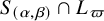 and we may therefore rewrite

Since
$\varpi \nmid B(\boldsymbol {c})$
 , the reduction of
$\boldsymbol {c}$
, the reduction of
$\boldsymbol {c}$
 modulo
$\varpi $
modulo
$\varpi $
 is good and hence the reduction of the binary form
$g_{\boldsymbol {c}}$
is good and hence the reduction of the binary form
$g_{\boldsymbol {c}}$
 modulo
$\varpi $
modulo
$\varpi $
 is separable of degree 6. Moreover, by construction
$S_{(\alpha :\beta )}$
is separable of degree 6. Moreover, by construction
$S_{(\alpha :\beta )}$
 will be singular precisely when
$\varpi \mid g_{\boldsymbol {c}}(\alpha ,\beta )$
will be singular precisely when
$\varpi \mid g_{\boldsymbol {c}}(\alpha ,\beta )$
 , since
$g_{\boldsymbol {c}}(\alpha ,\beta )$
, since
$g_{\boldsymbol {c}}(\alpha ,\beta )$
 is just the determinant of the matrix underlying the quadratic form defining
$S_{(\alpha :\beta )}$
is just the determinant of the matrix underlying the quadratic form defining
$S_{(\alpha :\beta )}$
 . Let
$\chi \colon \mathbb {F}_\varpi ^\times \to \mathbb {C}^\times $
. Let
$\chi \colon \mathbb {F}_\varpi ^\times \to \mathbb {C}^\times $
 be the unique character of order 2. It follows from Schmidt [Reference Schmidt47, § IV.2] that

provided
$\varpi \nmid g_{\boldsymbol {c}}(\alpha ,\beta )$
 . Let
$0\leqslant N_0 \leqslant 6$
. Let
$0\leqslant N_0 \leqslant 6$
 be the number of
$(\alpha :\beta )\in \mathbb {P}^1(\mathbb {F}_\varpi )$
be the number of
$(\alpha :\beta )\in \mathbb {P}^1(\mathbb {F}_\varpi )$
 such that
$\varpi \mid g_{\boldsymbol {c}}(\alpha ,\beta )$
such that
$\varpi \mid g_{\boldsymbol {c}}(\alpha ,\beta )$
 . It then follows that

where the
$O(|\varpi |)$
 term accounts for summing the
$+1$
term accounts for summing the
$+1$
 in Schmidt’s formula and the contribution from those
$(\alpha :\beta )$
in Schmidt’s formula and the contribution from those
$(\alpha :\beta )$
 with
$\beta =0$
with
$\beta =0$
 . The second line follows from the classical Weil bound for character sums, which is applicable since
$g_{\boldsymbol {c}}(t,1)$
. The second line follows from the classical Weil bound for character sums, which is applicable since
$g_{\boldsymbol {c}}(t,1)$
 is square-free modulo
$\varpi $
is square-free modulo
$\varpi $
 .
.
As the reduction of
$\boldsymbol {c}$
 modulo
$\varpi $
modulo
$\varpi $
 is good, we know from Lemma 10.4 that the matrix underlying the quadratic form defining
$S_{(\alpha :\beta )}$
is good, we know from Lemma 10.4 that the matrix underlying the quadratic form defining
$S_{(\alpha :\beta )}$
 has rank at least 3. In particular,
$S_{(\alpha :\beta )}$
has rank at least 3. In particular,
$S_{(\alpha :\beta )}$
 is irreducible and by Lang-Weil we get
$\#S_{(\alpha :\beta )}(\mathbb {F}_\varpi )=|\varpi |^2 +O(|\varpi |^{3/2})$
is irreducible and by Lang-Weil we get
$\#S_{(\alpha :\beta )}(\mathbb {F}_\varpi )=|\varpi |^2 +O(|\varpi |^{3/2})$
 . Thus

Finally, observe that since
$\varpi \nmid B(\boldsymbol {c})$
 , property (iii) in Definition 10.2 implies that there are at most 3 possible
$(\alpha :\beta )\in \mathbb {P}^1(\mathbb {F}_\varpi )$
, property (iii) in Definition 10.2 implies that there are at most 3 possible
$(\alpha :\beta )\in \mathbb {P}^1(\mathbb {F}_\varpi )$
 for which
$C_{(\alpha :\beta )}$
for which
$C_{(\alpha :\beta )}$
 is singular. If
$C_{(\alpha :\beta )}$
is singular. If
$C_{(\alpha :\beta )}$
 is smooth, then it contains
$|\varpi |+1\, \mathbb {F}_\varpi $
is smooth, then it contains
$|\varpi |+1\, \mathbb {F}_\varpi $
 -points, while if it is singular it is either a double line or a union of two lines, so that in either case it contains
$O(|\varpi |)\, \mathbb {F}_\varpi $
-points, while if it is singular it is either a double line or a union of two lines, so that in either case it contains
$O(|\varpi |)\, \mathbb {F}_\varpi $
 -points. Therefore,

Combining these estimates with the fact that
$\#L_\varpi (\mathbb {F}_\varpi )=|\varpi |^2+|\varpi |+1$
 , it follows from (10.5) that

Moreover, by Deligne’s bounds (as recorded in Equation (3.12) and the paragraph thereafter of [Reference Browning and Vishe12]), we have
$\#\mathcal {V}(\mathbb {F}_\varpi )= |\varpi |^4+|\varpi |^3 +O(|\varpi |^2)$
 . Thus (10.3) yields

On dividing both sides by
$|\varpi |^{7/2}$
 , we are led to the statement of the proposition.
Motivated by the previous result, for good
$\boldsymbol {c}\in L^\perp \setminus \{\boldsymbol {0}\}$
 we define

and observe that these sets depend implicitly on L. Moreover, it will be convenient to introduce the notation

for any integer
$l\geqslant 1$
 .
.
10.3 A general upper bound
Having completed the treatment of individual exponential sums, we will now focus on our case of interest and assume that

for the rest of this section. Recall the definition (2.13) of
$\mathcal {S}_0$
 . For each set
$\mathcal {T}\subseteq \mathcal {S}_0$
. For each set
$\mathcal {T}\subseteq \mathcal {S}_0$
 , let
, let

At several points later, it will be convenient to discard
$f(\mathcal {T})$
 for various choices of
$\mathcal {T}$
for various choices of
$\mathcal {T}$
 . This is achieved through the following result (which is analogous to [Reference Wang56, Lemma 5.2]).
Lemma 10.7. Let
$\mathcal {T}\subseteq \mathcal {S}_0$
 and
$\delta \in \mathbb {R}$
and
$\delta \in \mathbb {R}$
 . Suppose
$\{\lambda \boldsymbol {c}: (\lambda , \boldsymbol {c})\in K^\times \times \mathcal {T}\} \cap \mathcal {O}^n = \mathcal {T}$
. Suppose
$\{\lambda \boldsymbol {c}: (\lambda , \boldsymbol {c})\in K^\times \times \mathcal {T}\} \cap \mathcal {O}^n = \mathcal {T}$
 and
$\#{\{\boldsymbol {c}\in \mathcal {T}: \lvert \boldsymbol {c} \rvert \leqslant \widehat C\}}=O(\widehat C^{n-3-\delta })$
and
$\#{\{\boldsymbol {c}\in \mathcal {T}: \lvert \boldsymbol {c} \rvert \leqslant \widehat C\}}=O(\widehat C^{n-3-\delta })$
 for all
$C\in \mathbb {R}_{\geqslant 0}$
for all
$C\in \mathbb {R}_{\geqslant 0}$
 . Assume
$\delta \leqslant \frac 52$
. Assume
$\delta \leqslant \frac 52$
 . Then

for any
$\varepsilon>0$
 .
.
Proof. The result [Reference Glas and Hochfilzer26, Lemma 6.1] essentially gives a version of this result with
$\delta <0$
 , and with
$s=r$
, and with
$s=r$
 instead of
$\sum _{s\mid r}$
instead of
$\sum _{s\mid r}$
 . The same method extends to the present setting, with minor modifications that we now describe.
First, the integral estimate [Reference Glas and Hochfilzer26, Eq. (6.9)] still holds. (In fact, we have seen that the stronger estimate (8.2) is available.) Second, taking
$n=6$
 , we have

in the notation of [Reference Glas and Hochfilzer26]. Therefore,

since
$s_2\mid r_2$
 and
$s_3\mid r_3$
and
$s_3\mid r_3$
 . This is of the exact same strength as the bound for the
$s=r$
. This is of the exact same strength as the bound for the
$s=r$
 term given in [Reference Glas and Hochfilzer26, Lemma 6.1]. Since
$-\frac 52 + \delta \leqslant 0$
term given in [Reference Glas and Hochfilzer26, Lemma 6.1]. Since
$-\frac 52 + \delta \leqslant 0$
 , the rest of the argument of [Reference Glas and Hochfilzer26] goes through with
$-\delta $
, the rest of the argument of [Reference Glas and Hochfilzer26] goes through with
$-\delta $
 in place of
$\eta $
in place of
$\eta $
 to give the desired upper bound for
$f(\mathcal {T})$
to give the desired upper bound for
$f(\mathcal {T})$
 . Here our assumption on
$\mathcal {T}$
. Here our assumption on
$\mathcal {T}$
 guarantees that if
$H\boldsymbol {c}\in \mathcal {T}$
guarantees that if
$H\boldsymbol {c}\in \mathcal {T}$
 for some
$\boldsymbol {c}\in \mathcal {O}^n$
for some
$\boldsymbol {c}\in \mathcal {O}^n$
 and
$H\in \mathcal {O}\setminus \{0\}$
and
$H\in \mathcal {O}\setminus \{0\}$
 , then in fact we have
$\boldsymbol {c}\in \mathcal {T}$
, then in fact we have
$\boldsymbol {c}\in \mathcal {T}$
 . This implies that

which is all that is used to arrive at [Reference Glas and Hochfilzer26, Eq. (6.10)].
10.4 Factorising exponential sums
Given the bias established in Proposition 10.6, we typically expect
$S^\natural _r(\boldsymbol {c})$
 to be of size
$|r|^{1/2}$
to be of size
$|r|^{1/2}$
 for
$\boldsymbol {c}\in \Lambda ^\perp $
for
$\boldsymbol {c}\in \Lambda ^\perp $
 , at least when r is square-free. To keep track of the error, we will decompose
$S_r^\natural (\boldsymbol {c})$
, at least when r is square-free. To keep track of the error, we will decompose
$S_r^\natural (\boldsymbol {c})$
 into smaller pieces.
For
$r\in \mathcal {O}$
 , let
$\phi _K(r)=\#(\mathcal {O}/r\mathcal {O})^\times $
, let
$\phi _K(r)=\#(\mathcal {O}/r\mathcal {O})^\times $
 be the Euler totient function. Consider the Dirichlet series

In the notation of (4.1), it follows from Proposition 10.6 that the local factor
$\Phi _\varpi (\boldsymbol {c},s)$
 should resemble the local factor
$\Psi _\varpi (s)$
should resemble the local factor
$\Psi _\varpi (s)$
 of
$\Psi (s)$
of
$\Psi (s)$
 . Let
$S_{r,0}(\boldsymbol {c})$
. Let
$S_{r,0}(\boldsymbol {c})$
 be the rth coefficient of the Euler product
$\Phi (\boldsymbol {c},s)/\Psi (s)$
be the rth coefficient of the Euler product
$\Phi (\boldsymbol {c},s)/\Psi (s)$
 ; then

Since
$\mu _K(r)$
 is the rth coefficient of
$\zeta _K(s)^{-1} = \prod _\varpi (1-\lvert \varpi \rvert ^{-s})$
is the rth coefficient of
$\zeta _K(s)^{-1} = \prod _\varpi (1-\lvert \varpi \rvert ^{-s})$
 , it follows upon expanding products that

Moreover, the Euler product factorisation
$\Phi = (\Phi /\Psi ) \cdot \Psi $
 implies

We will need some basic properties of
$S_{r,0}(\boldsymbol {c})$
 as a function of
$\boldsymbol {c}\in \Lambda ^\perp $
as a function of
$\boldsymbol {c}\in \Lambda ^\perp $
 and
$r\in \mathcal {O}^+$
and
$r\in \mathcal {O}^+$
 .
.
Lemma 10.8. The quantity
$S_{r,0}(\boldsymbol {c})$
 is multiplicative in r and only depends on
$\boldsymbol {c}\bmod {r}$
is multiplicative in r and only depends on
$\boldsymbol {c}\bmod {r}$
 . Also,

Proof. Being the convolution of multiplicative functions, the multiplicativity is clear. Moreover, from (10.8) it follows that
$S_{r,0}(\boldsymbol {c})$
 depends only on the list of values
$\boldsymbol {c} \bmod d$
depends only on the list of values
$\boldsymbol {c} \bmod d$
 for divisors d of r, which in turn implies that
$S_{r,0}(\boldsymbol {c})$
for divisors d of r, which in turn implies that
$S_{r,0}(\boldsymbol {c})$
 only depends on
$\boldsymbol {c}\bmod r$
only depends on
$\boldsymbol {c}\bmod r$
 . Finally, by orthogonality of characters we have

so that the last assertion follows from the formal identity

which follows from (10.7).
We now provide some bounds for
$S_{r,0}(\boldsymbol {c})$
 for
$\boldsymbol {c}\in \Lambda ^\perp \setminus \{\boldsymbol {0}\}$
for
$\boldsymbol {c}\in \Lambda ^\perp \setminus \{\boldsymbol {0}\}$
 .
.
Lemma 10.9. Let
$r\in \mathcal {O}^+$
 ,
$\boldsymbol {c}\in \Lambda ^\perp \setminus \{\boldsymbol {0}\}$
,
$\boldsymbol {c}\in \Lambda ^\perp \setminus \{\boldsymbol {0}\}$
 and let
$\varepsilon>0$
and let
$\varepsilon>0$
 . Then

Moreover, if
$B(\boldsymbol {c})\neq 0$
 and r is a square-free element of
${\mathcal{N}_{\boldsymbol{c}}^{\text{G}}} $
and r is a square-free element of
${\mathcal{N}_{\boldsymbol{c}}^{\text{G}}} $
 , then
$ S_{r,0}(\boldsymbol {c})\ll _\varepsilon |r|^{\varepsilon }. $
, then
$ S_{r,0}(\boldsymbol {c})\ll _\varepsilon |r|^{\varepsilon }. $

Proof. Applying the triangle inequality in (10.8), followed by Lemma 6.1 to cube-free divisors of r, we obtain

which verifies the first part. If
$\varpi \nmid B(\boldsymbol {c})$
 , then (10.8), Proposition 10.6 and Lemma 10.8 together imply
$ S_{\varpi ,0}(\boldsymbol {c}) = -\lvert \varpi \rvert ^{1/2} + \lvert \varpi \rvert ^{-1/2} + S^\natural _\varpi (\boldsymbol {c}) \ll 1$
, then (10.8), Proposition 10.6 and Lemma 10.8 together imply
$ S_{\varpi ,0}(\boldsymbol {c}) = -\lvert \varpi \rvert ^{1/2} + \lvert \varpi \rvert ^{-1/2} + S^\natural _\varpi (\boldsymbol {c}) \ll 1$
 . The second assertion now follows from multiplicativity.
We shall also require the following estimate for averages of
$S_{r,0}(\boldsymbol {c})$
 .
.
Lemma 10.10. Let
$\varepsilon>0$
 . Let
$\boldsymbol {c}\in \Lambda ^\perp \setminus \{\boldsymbol {0}\}$
. Let
$\boldsymbol {c}\in \Lambda ^\perp \setminus \{\boldsymbol {0}\}$
 be such that
$B(\boldsymbol {c})\neq 0$
be such that
$B(\boldsymbol {c})\neq 0$
 and
$R\geqslant 0$
and
$R\geqslant 0$
 . Then
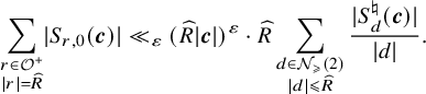
Proof. Any
$r\in \mathcal {O}^+$
 can be written uniquely as
$r_1r_2r_3$
can be written uniquely as
$r_1r_2r_3$
 , where
$r_1,r_2,r_3\in \mathcal {O}^+$
, where
$r_1,r_2,r_3\in \mathcal {O}^+$
 are pairwise coprime with
$r_1\in {\mathcal{N}_{\boldsymbol{c}}^{\text{G}}} $
are pairwise coprime with
$r_1\in {\mathcal{N}_{\boldsymbol{c}}^{\text{G}}} $
 square-free,
$r_2\in {\mathcal{N}_{\boldsymbol{c}}^{\text{B}}} $
square-free,
$r_2\in {\mathcal{N}_{\boldsymbol{c}}^{\text{B}}} $
 square-free and
$r_3$
square-free and
$r_3$
 square-full. Upon writing
$S_{r,0}(\boldsymbol {c}) = \prod _{1\leqslant i\leqslant 3} S_{r_i,0}(\boldsymbol {c})$
square-full. Upon writing
$S_{r,0}(\boldsymbol {c}) = \prod _{1\leqslant i\leqslant 3} S_{r_i,0}(\boldsymbol {c})$
 , and applying Lemma 10.9 to each factor, we get after decomposing into q-adic intervals

Since
$B(\boldsymbol {c})\neq 0$
 and
$|B(\boldsymbol {c})|\ll |\boldsymbol {c}|^{O(1)}$
and
$|B(\boldsymbol {c})|\ll |\boldsymbol {c}|^{O(1)}$
 , it follows from Lemma 2.2 that the number of
$r_2\in {\mathcal{N}_{\boldsymbol{c}}^{\text{B}}} $
, it follows from Lemma 2.2 that the number of
$r_2\in {\mathcal{N}_{\boldsymbol{c}}^{\text{B}}} $
 with
$|r_2|=\widehat {R}_2$
with
$|r_2|=\widehat {R}_2$
 is
$O_\varepsilon ((|\boldsymbol {c}|\widehat {R}_2)^\varepsilon )$
is
$O_\varepsilon ((|\boldsymbol {c}|\widehat {R}_2)^\varepsilon )$
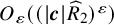 . In particular, we get, after summing over the
$r_i$
. In particular, we get, after summing over the
$r_i$
 for each fixed d, that the right-hand side is

Lemma 10.10 follows, since
$\widehat R_1 \widehat R_2^{1/2} \widehat R_3^{1/2} \widehat R_3^{1/2} \leqslant \widehat R_1\widehat R_2\widehat R_3 = \widehat R$
 .
.
10.5 Linear space extraction
By an
$\mathbb {F}_q$
 -linear change of variables, when studying linear spaces
$L\in \Upsilon $
-linear change of variables, when studying linear spaces
$L\in \Upsilon $
 we may concentrate on
$L=L_0$
we may concentrate on
$L=L_0$
 , as given by (10.2). Elements of
$L_0^\perp $
, as given by (10.2). Elements of
$L_0^\perp $
 are of the shape
$(c_1,c_2,c_3,c_1,c_2,c_3)$
are of the shape
$(c_1,c_2,c_3,c_1,c_2,c_3)$
 for
$\boldsymbol {c}=(c_1,c_2,c_3)\in \mathcal {O}^3$
for
$\boldsymbol {c}=(c_1,c_2,c_3)\in \mathcal {O}^3$
 . Motivated by this, we define
$\boldsymbol {c}^*=(c_1,c_2,c_3,c_1,c_2,c_3)$
. Motivated by this, we define
$\boldsymbol {c}^*=(c_1,c_2,c_3,c_1,c_2,c_3)$
 for
$\boldsymbol {c}\in \mathcal {O}^3$
for
$\boldsymbol {c}\in \mathcal {O}^3$
 .
.
Our next result will allow us to extract the main contribution from solutions on linear subspaces to our counting function. Before stating it, we need some more notation. Given
$\boldsymbol {x}\in \mathcal {O}^6$
 , set
, set

for
$i=1,2,3$
 . Moreover, we let
$M\in \operatorname {\mathrm {GL}}_6(\mathcal {O})$
. Moreover, we let
$M\in \operatorname {\mathrm {GL}}_6(\mathcal {O})$
 be such that
$\boldsymbol {x}=M(\boldsymbol {y},\boldsymbol {z})$
be such that
$\boldsymbol {x}=M(\boldsymbol {y},\boldsymbol {z})$
 . We then define the cubic form

and the density
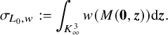
Note that
$M(\boldsymbol {0},\boldsymbol {z})=\frac {1}{2}(z_1,z_2,z_3,-z_1,-z_2,-z_3)$
 , so that
$\sigma _{L_0,w}$
, so that
$\sigma _{L_0,w}$
 measures the density of
$K_\infty $
measures the density of
$K_\infty $
 -points on the lattice
$\Lambda _0$
-points on the lattice
$\Lambda _0$
 with respect to w.
Lemma 10.11. Let
$\boldsymbol {c}_0\in \mathcal {O}^3$
 and assume that
$r=r_0r_1\in \mathcal {O}^+$
and assume that
$r=r_0r_1\in \mathcal {O}^+$
 . There exists a constant
$C\in \mathbb {N}$
. There exists a constant
$C\in \mathbb {N}$
 such that if
$|r_1|\geqslant \widehat {C}|P|$
such that if
$|r_1|\geqslant \widehat {C}|P|$
 , then
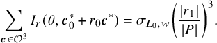
Proof. Upon making the unimodular change of variables
$\boldsymbol {x}\mapsto (\boldsymbol {y}, \boldsymbol {z})$
 described above, we get that

Applying another change of variables given by
$\boldsymbol {y}'=P\boldsymbol {y}/r_1$
 , we obtain

where
$\widehat {g}_{\boldsymbol {z}}$
 is the Fourier transform of the function

In particular, using Poisson summation, in the form Lemma 2.1, we deduce that

Suppose that
$\boldsymbol {b}\neq \boldsymbol {0}$
 . Then, since we may assume
$|r_1|\geqslant \widehat {C}|P|$
. Then, since we may assume
$|r_1|\geqslant \widehat {C}|P|$
 for a sufficiently large constant C, we must have
$w(M(r_1\boldsymbol {b}/P,\boldsymbol {z}))=0$
for a sufficiently large constant C, we must have
$w(M(r_1\boldsymbol {b}/P,\boldsymbol {z}))=0$
 . It follows that only the term
$\boldsymbol {b}=\boldsymbol {0}$
. It follows that only the term
$\boldsymbol {b}=\boldsymbol {0}$
 contributes. However, we have
$\widetilde {F}(\boldsymbol {0},\boldsymbol {z})=0$
contributes. However, we have
$\widetilde {F}(\boldsymbol {0},\boldsymbol {z})=0$
 identically in
$\boldsymbol {z}$
identically in
$\boldsymbol {z}$
 , so that we arrive at the statement of the lemma.
10.6 Proof of Proposition 10.1
We will now combine all the results we have obtained so far to complete the proof of Proposition 10.1. For
$\mathcal {E}\subset \mathcal {O}^6$
 , we set

Then
$S(\mathcal {S}_0)= E_2(P)$
 , so that Proposition 10.1 can be rephrased as

Let us define

where
$B\in \mathcal {O}[x_1,x_2,x_3]$
 is the form in the statement of Proposition 10.6.
Lemma 10.12. For any
$C\geqslant 1$
 and
$L\in \Upsilon $
and
$L\in \Upsilon $
 , we have

Proof. Since
$B\in \mathcal {O}[x_1,x_2,x_3]$
 is a nonzero form, we get from Lemma 2.10 that the contribution from
$\boldsymbol {c}\in \mathcal {E}_2(L)$
is a nonzero form, we get from Lemma 2.10 that the contribution from
$\boldsymbol {c}\in \mathcal {E}_2(L)$
 with
$B(\boldsymbol {c})=0$
with
$B(\boldsymbol {c})=0$
 is
$O(\widehat {C}^2)$
is
$O(\widehat {C}^2)$
 . Moreover, any
$\boldsymbol {c}\in \Lambda ^\perp $
. Moreover, any
$\boldsymbol {c}\in \Lambda ^\perp $
 takes the shape
$(c_1, c_2, c_3, c_1, c_2, c_3)$
takes the shape
$(c_1, c_2, c_3, c_1, c_2, c_3)$
 for some
$(c_1,c_2,c_3)\in \mathcal {O}^3$
for some
$(c_1,c_2,c_3)\in \mathcal {O}^3$
 . From this description it immediately follows that the contribution from
$\boldsymbol {c}\in \Lambda ^\perp $
. From this description it immediately follows that the contribution from
$\boldsymbol {c}\in \Lambda ^\perp $
 with
$c_1\cdots c_6=0$
with
$c_1\cdots c_6=0$
 is
$O(\widehat {C}^2)$
is
$O(\widehat {C}^2)$
 .
.
For
$\boldsymbol {c}\in \mathcal {E}_1$
 , this is already implicit in the proof of Lemma 5.1 of [Reference Glas and Hochfilzer26] and so we shall be brief. Let
$m_{1},\dots , m_{k}\in \mathcal {O}$
, this is already implicit in the proof of Lemma 5.1 of [Reference Glas and Hochfilzer26] and so we shall be brief. Let
$m_{1},\dots , m_{k}\in \mathcal {O}$
 with
$1\leqslant k \leqslant 6$
with
$1\leqslant k \leqslant 6$
 be square-free and either monic or with leading coefficient a primitive root of
$\mathbb {F}_q^\times $
be square-free and either monic or with leading coefficient a primitive root of
$\mathbb {F}_q^\times $
 . Suppose that
$\boldsymbol {c}\in \mathcal {O}^6$
. Suppose that
$\boldsymbol {c}\in \mathcal {O}^6$
 satisfies
$F^*(\boldsymbol {c})=0$
satisfies
$F^*(\boldsymbol {c})=0$
 . We then partition
$\{1,\dots , 6\}$
. We then partition
$\{1,\dots , 6\}$
 into sets
$\mathcal {I}(1),\dots , \mathcal {I}(k)$
into sets
$\mathcal {I}(1),\dots , \mathcal {I}(k)$
 , where
$i\in \mathcal {I}(j)$
, where
$i\in \mathcal {I}(j)$
 if and only if
$c_i^3=m_jd_i^2$
if and only if
$c_i^3=m_jd_i^2$
 for some
$d_i\in \mathcal {O}$
for some
$d_i\in \mathcal {O}$
 . It then follows from the last display in the proof of Lemma 5.1 of [Reference Glas and Hochfilzer26] that the contribution from all
$\boldsymbol {c}\in \mathcal {O}^6$
. It then follows from the last display in the proof of Lemma 5.1 of [Reference Glas and Hochfilzer26] that the contribution from all
$\boldsymbol {c}\in \mathcal {O}^6$
 ranging over all permissible
$m_1,\dots , m_k$
ranging over all permissible
$m_1,\dots , m_k$
 is
$O_\varepsilon (\widehat {C}^{2+\varepsilon })$
is
$O_\varepsilon (\widehat {C}^{2+\varepsilon })$
 unless
$k=3$
unless
$k=3$
 and
$\#\mathcal {I}(1)=\#\mathcal {I}(2)=\#\mathcal {I}(3)=2$
and
$\#\mathcal {I}(1)=\#\mathcal {I}(2)=\#\mathcal {I}(3)=2$
 . If the latter holds, then the display after (5.1) in the proof of Lemma 5.1 of [Reference Glas and Hochfilzer26] gives
$d_{i_1}=-d_{i_2}$
. If the latter holds, then the display after (5.1) in the proof of Lemma 5.1 of [Reference Glas and Hochfilzer26] gives
$d_{i_1}=-d_{i_2}$
 for
$\mathcal {I}(j)=\{i_1,i_2\}$
for
$\mathcal {I}(j)=\{i_1,i_2\}$
 and
$j=1,2,3$
and
$j=1,2,3$
 , which in turn implies
$c_{i_1}^3=c^3_{i_2}$
, which in turn implies
$c_{i_1}^3=c^3_{i_2}$
 and hence
$\boldsymbol {c}$
and hence
$\boldsymbol {c}$
 lies in
$\Lambda ^\perp $
lies in
$\Lambda ^\perp $
 for some
$L\in \Upsilon $
for some
$L\in \Upsilon $
 .
.
Note that for any distinct
$L_1,L_2\in \Upsilon $
 , we have

In particular, applying Lemma 10.7 twice, with
$\delta =1-\varepsilon $
 , in conjunction with Lemma 10.12, we obtain

Note that since any
$L_1, L_2\in \Upsilon $
 are isomorphic under an
$\mathbb {F}_q$
are isomorphic under an
$\mathbb {F}_q$
 -linear map, we may concentrate on the contribution from
$L=L_0$
-linear map, we may concentrate on the contribution from
$L=L_0$
 . In particular, Proposition 10.1 will follow once we have established

where
$\mathcal {E}_2=\mathcal {E}_2(L_0)$
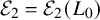 . Indeed, the only step that needs explaining is the equality

However, this counting result is standard (with a much better error term) and we omit the proof.
For a real number
$U>0$
 and a set
$\mathcal {T}\subseteq \mathcal {O}^6$
and a set
$\mathcal {T}\subseteq \mathcal {O}^6$
 , let
, let

Similarly we define
$\Sigma _{\geqslant U}(P, \mathcal {T})$
 by replacing
$\lvert r_1 \rvert <U$
by replacing
$\lvert r_1 \rvert <U$
 with
$\lvert r_1 \rvert \geqslant U$
with
$\lvert r_1 \rvert \geqslant U$
 . For a parameter
$W\geqslant 1$
. For a parameter
$W\geqslant 1$
 , to be chosen in due course, (10.9) allows us to rewrite the left-hand side of (10.10) as

We will complete the proof of Proposition 10.1 with the following three results.
Lemma 10.13. For any real
$W\geqslant 1$
 , we have

Proof. Since
$I_r(\boldsymbol {c})\ne 0$
 only for
$|\boldsymbol {c}|\ll \lvert P \rvert ^{1/2}$
only for
$|\boldsymbol {c}|\ll \lvert P \rvert ^{1/2}$
 , it follows that

We now examine an individual
$\boldsymbol {c}\in \Lambda _0^\perp \setminus \mathcal {E}_2$
 . Since
$c_1\cdots c_6\neq 0$
. Since
$c_1\cdots c_6\neq 0$
 , it follows from (8.2) that

Recall that any element of
$\Lambda _0^\perp $
 takes the shape
$(c_1,c_2, c_{3},c_1,c_2, c_{3})$
takes the shape
$(c_1,c_2, c_{3},c_1,c_2, c_{3})$
 . Let us now consider the contribution from those
$r_0$
. Let us now consider the contribution from those
$r_0$
 with
$|r_0|=\widehat {R}_0$
with
$|r_0|=\widehat {R}_0$
 . Upon inserting (10.13) and then applying Lemma 10.10, we find that the contribution to the quantity
$\Sigma _{<\widehat {Q}/\widehat {W}}(P, \Lambda _0^\perp \setminus \mathcal {E}_2)$
. Upon inserting (10.13) and then applying Lemma 10.10, we find that the contribution to the quantity
$\Sigma _{<\widehat {Q}/\widehat {W}}(P, \Lambda _0^\perp \setminus \mathcal {E}_2)$
 is
is

We also have
$S^\natural _d(\boldsymbol {c}) \ll _\varepsilon \lvert d \rvert ^{1/2+\varepsilon } \prod _{1\leqslant i\leqslant 3} \lvert \text {sq}(c_i) \rvert ^{1/2}$
 by Lemma 6.2, and
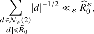
so that the last display is

Since
$\sum _{0<\lvert c \rvert \leqslant \widehat C} \lvert \text {sq}(c) \rvert ^{1/2}/\lvert c \rvert \ll _\varepsilon \widehat C^\varepsilon $
 , this becomes

Recalling that
$\widehat {Q} \asymp \lvert P \rvert ^{3/2}$
 and that there are
$O_\varepsilon (\widehat {Q}^\varepsilon )=O_\varepsilon (|P|^\varepsilon )$
and that there are
$O_\varepsilon (\widehat {Q}^\varepsilon )=O_\varepsilon (|P|^\varepsilon )$
 choices for
$R_0$
choices for
$R_0$
 completes the proof.
In the light of Lemma 10.11, we make the choice

We now turn to the range
$\lvert r_1 \rvert \geqslant \widehat {Q}/\widehat {W}$
 in (10.12).
Lemma 10.14. We have

Proof. By the first part of Lemma 10.8,
$S_{r_0,0}(\boldsymbol {c})$
 only depends on
$\boldsymbol {c}\bmod {r_0}$
only depends on
$\boldsymbol {c}\bmod {r_0}$
 . If
$\lvert r_1 \rvert \geqslant \widehat {Q}/\widehat {W} = \widehat {C}\lvert P \rvert $
. If
$\lvert r_1 \rvert \geqslant \widehat {Q}/\widehat {W} = \widehat {C}\lvert P \rvert $
 , then after splitting
$\boldsymbol {c}$
, then after splitting
$\boldsymbol {c}$
 into residue classes, Lemma 10.11 implies that

By Lemma 10.8 and the equality
$\#{ \Lambda _0^\perp /r_0\Lambda _0^\perp } = |r_0|^{3}$
 , we conclude that

We have therefore established the identity

However, by Dirichlet’s approximation theorem (2.2) we have

which completes the proof.
Lemma 10.15. We have

Proof. The main subtlety here is that we must treat
$\boldsymbol {c}\neq \boldsymbol {0}$
 and
$\boldsymbol {c}=\boldsymbol {0}$
and
$\boldsymbol {c}=\boldsymbol {0}$
 separately. First, given
$r\in \mathcal {O}^+$
separately. First, given
$r\in \mathcal {O}^+$
 , we apply the triangle inequality and the trivial divisor estimate to (10.8), giving

Inserting (10.15) into the definition (10.11) of
$\Sigma _{\geqslant \widehat {Q}/\widehat {W}}(X, \mathcal {E}_2\setminus \{\boldsymbol {0}\})$
 and recalling the definition (10.6) of f, we get

On combining Lemma 10.7 with the choice
$\delta =1-\varepsilon $
 in Lemma 10.12, we deduce that
$f(\mathcal {E}_2)\ll _\varepsilon |P|^{3-1/2+\varepsilon }$
in Lemma 10.12, we deduce that
$f(\mathcal {E}_2)\ll _\varepsilon |P|^{3-1/2+\varepsilon }$
 , which is satisfactory since
$\widehat {Q}= |P|^{3/2}$
, which is satisfactory since
$\widehat {Q}= |P|^{3/2}$
 . Similarly, (10.15) gives

which is
$O_\varepsilon (|P|^{3+\varepsilon } (\widehat {Q}/\widehat {W})^{-2/3+\varepsilon })$
 by (8.2) and Lemma 9.2 summed over q-adic ranges for
$|r|$
by (8.2) and Lemma 9.2 summed over q-adic ranges for
$|r|$
 . Since
$\widehat Q/\widehat W\gg |P|$
. Since
$\widehat Q/\widehat W\gg |P|$
 , we conclude that
$|P|^{3}(\widehat {Q}/\widehat {W})^{-2/3 } \ll |P|^{3 -2/3 }$
, we conclude that
$|P|^{3}(\widehat {Q}/\widehat {W})^{-2/3 } \ll |P|^{3 -2/3 }$
 .
.
Recalling our choice for
$\widehat {W}$
 in (10.14), we see that (10.10) follows from inserting Lemmas 10.13–10.15 into (10.12). This finally completes the proof of Proposition 10.1.
11 Final reckoning
11.1 Proof of Theorem 1.1
Let
$F(\boldsymbol x)=x_1^3+\cdots +x_6^3$
 and let
$w_{\boldsymbol {x}_0}$
and let
$w_{\boldsymbol {x}_0}$
 be the weight function defined in Definition 5.4, associated to an appropriate
$\boldsymbol {x}_0\in (\mathbb {F}_q^\times )^6$
be the weight function defined in Definition 5.4, associated to an appropriate
$\boldsymbol {x}_0\in (\mathbb {F}_q^\times )^6$
 . Then we have

for any
$P\in \mathcal {O}$
 , in the notation of (1.1) and (2.4). Let
$L(s,\boldsymbol c)$
, in the notation of (1.1) and (2.4). Let
$L(s,\boldsymbol c)$
 be the Hasse–Weil L-function introduced in § 3, for
$\boldsymbol {c}\in \mathcal {O}^6$
be the Hasse–Weil L-function introduced in § 3, for
$\boldsymbol {c}\in \mathcal {O}^6$
 . Theorem 1.1 relies on the Ratios Conjecture for these L-functions, as
$\boldsymbol {c}$
. Theorem 1.1 relies on the Ratios Conjecture for these L-functions, as
$\boldsymbol {c}$
 varies. We have seen several forms of the Ratios Conjecture during the course of the paper. The following result is a stronger version of Theorem 1.1, and makes clear the various interdependencies.
Theorem 11.1. Assume
$\operatorname {\mathrm {char}}(\mathbb {F}_q)>3$
 . Then each of the following implies the next:
-
1. The Ratios Conjecture 3.6 (R2), for shifted second moments of $1/L(s,\boldsymbol {c})$
. -
2. Conjecture 3.7 holds.
-
3. Conjecture 3.8 holds.
-
4. Conjecture 4.5 holds.
-
5. $N(P)\ll _q |P|^3$
for any
$P\in \mathcal {O}$
. -
6. If $S\subseteq \mathcal {O}$
has positive lower density, then so does
$\{x^3+y^3+z^3: x,y,z\in S\}$
. -
7. The set $\{k: x^3+y^3+z^3=k\text { is soluble in } \mathcal {O}^+ \text { with } \text {max}\{\lvert x \rvert ,\lvert y \rvert ,\lvert z \rvert \} = \lvert k \rvert ^{1/3}\}$
has positive lower density.






Proof. We gave a proof that Conjecture 3.7 follows from the Ratios Conjecture (R2) directly after the annunciation of the conjecture, so that (1)
$\Rightarrow $
 (2). Similarly for the deduction of Conjecture 3.8 from Conjecture 3.7, whence (2)
$\Rightarrow $
(2). Similarly for the deduction of Conjecture 3.8 from Conjecture 3.7, whence (2)
$\Rightarrow $
 (3), and for the deduction of Conjecture 4.5 from Conjecture 3.8, whence (3)
$\Rightarrow $
(3), and for the deduction of Conjecture 4.5 from Conjecture 3.8, whence (3)
$\Rightarrow $
 (4). These implications mostly lie in the world of L-functions.
The implication (4)
$\Rightarrow $
 (5) requires the full force of the function field circle method. Combining (2.9) with the notation introduced in (8.1), (9.1) and (10.1), we see that

Assume that Conjecture 4.5 holds. Bearing in mind the bound (10.10) and the fact that
$\Upsilon $
 is finite, we may combine Propositions 8.1, 9.1 and 10.1 in order to conclude that
$N(P)\ll |P|^3$
is finite, we may combine Propositions 8.1, 9.1 and 10.1 in order to conclude that
$N(P)\ll |P|^3$
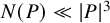 for any
$P\in \mathcal {O}$
for any
$P\in \mathcal {O}$
 .
.
The implication (6)
$\Rightarrow $
 (7) follows by taking
$S=\mathcal {O}^+$
(7) follows by taking
$S=\mathcal {O}^+$
 in (6). Indeed, in
$\mathcal {O}^+$
in (6). Indeed, in
$\mathcal {O}^+$
 we always have
$\deg (x^3+y^3+z^3) = 3\text { max}(\deg (x),\deg (y),\deg (z))$
we always have
$\deg (x^3+y^3+z^3) = 3\text { max}(\deg (x),\deg (y),\deg (z))$
 , since
$\operatorname {\mathrm {char}}(\mathbb {F}_q)> 3$
, since
$\operatorname {\mathrm {char}}(\mathbb {F}_q)> 3$
 .
.
Finally, we deal with the implication (5)
$\Rightarrow $
 (6). For any positive integer d, let

We wish to prove that
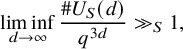
where the implied constant is allowed to depend on S and q. Since
$S\subseteq \mathcal {O}$
 has positive lower density, there exists
$A\in \mathbb {N}$
has positive lower density, there exists
$A\in \mathbb {N}$
 such that

Let
$S_e = \{x\in S: |x| = q^e\}$
 , for any
$e\in \mathbb {Z}_{\geqslant 0}$
, for any
$e\in \mathbb {Z}_{\geqslant 0}$
 . Then, for all sufficiently large integers d, we have
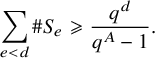
Since
$\sum _{e < d-A} \#S_e \leqslant q^{d-A}$
 , by trivially bounding
$\#S_e$
, by trivially bounding
$\#S_e$
 , we obtain

Thus, by the pigeonhole principle, there exists
$e = e(d) \in [d-A, d-1]$
 such that
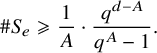
Given
$k\in \mathcal {O}$
 , we denote by
$r_S(k)$
, we denote by
$r_S(k)$
 the number of
$(x,y,z)\in S^3$
the number of
$(x,y,z)\in S^3$
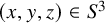 for which
$x^3+y^3+z^3=k$
for which
$x^3+y^3+z^3=k$
 and
$|x|= |y|=|z|= q^e$
and
$|x|= |y|=|z|= q^e$
 . Then it follows from Cauchy–Schwarz that

Part (5) implies that
$N(t^e)=O(q^{3e})$
 . Moreover, on the left hand side we have
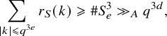
by (11.1). It now follows that
$U_S(d)\geqslant U_S(e)\gg _A q^{3d}$
 , which establishes part (6).
When
$F=x_1^3+\dots +x_6^3$
 , through careful use of Hölder’s inequality, it would be possible to replace the upper bound in (5) by
$N_F(w,P) \ll _w \lvert P \rvert ^3$
, through careful use of Hölder’s inequality, it would be possible to replace the upper bound in (5) by
$N_F(w,P) \ll _w \lvert P \rvert ^3$
 for any
$w\in S(K^n_\infty )$
for any
$w\in S(K^n_\infty )$
 . However, since doing so would make the paper needlessly longer, we have decided to omit the details here.
11.2 Possible reductions to Ratios
To facilitate a deeper discussion of the Ratios Conjecture, we make the following definition.
Definition 11.2. Let
$\mathcal {F}_q$
 be a geometric family of L-functions
$L(s,f)$
be a geometric family of L-functions
$L(s,f)$
 over
$\mathbb {F}_q(t)$
over
$\mathbb {F}_q(t)$
 , with a gauge function
$D(f)$
, with a gauge function
$D(f)$
 approximating the conductor, in the sense of [Reference Sarnak, Shin and Templier46, pp. 534–535]. Let
$\mathcal {Q} \subseteq \mathbb {Z}$
approximating the conductor, in the sense of [Reference Sarnak, Shin and Templier46, pp. 534–535]. Let
$\mathcal {Q} \subseteq \mathbb {Z}$
 . Assume
$\mathcal {F}_q$
. Assume
$\mathcal {F}_q$
 varies naturally with
$q\in \mathcal {Q}$
varies naturally with
$q\in \mathcal {Q}$
 , forming a family
$\mathcal {F} = (\mathcal {F}_q)_{q\in \mathcal {Q}}$
, forming a family
$\mathcal {F} = (\mathcal {F}_q)_{q\in \mathcal {Q}}$
 . We say that the q-restricted Ratios Conjecture holds if for any ratio average over
$D(f)\leqslant q^Z$
. We say that the q-restricted Ratios Conjecture holds if for any ratio average over
$D(f)\leqslant q^Z$
 , one has an asymptotic with power saving
$O_q(q^{-\delta Z})$
, one has an asymptotic with power saving
$O_q(q^{-\delta Z})$
 in the strip

where
$\delta>0$
 depends only on
$\mathcal {F}$
depends only on
$\mathcal {F}$
 ,
$\mathcal {Q}$
,
$\mathcal {Q}$
 and the ratio in question.
Note that one can also study the Ratios Conjecture in other aspects; see work of Bui–Florea–Keating [Reference Bui, Florea and Keating13], and work of Florea [Reference Florea22]. We shall prove in Theorem 11.4 that the q-restricted Ratios Conjecture suffices in Theorem 1.1, if q is large enough. The homological stability framework of [Reference Bergström, Diaconu, Petersen and Westerland5,Reference Miller, Patzt, Petersen and Randal-Williams43] might eventually resolve this particular form of the Ratios Conjecture for sufficiently large values of q. Evidence for this appears in work of Wang [Reference Wang55], in the simpler setting of (imaginary) quadratic Dirichlet L-functions.
Theorem 11.3 [Reference Wang55]
The q-restricted Ratios Conjecture holds for quadratic Dirichlet L-functions over
$\mathbb {F}_q(t)$
 , for odd q large enough in terms of the ratio in question.
The following result illustrates how a homological stability proof might impact the work of this paper. The specific term
$q^{-\delta }$
 in (11.2) is unimportant; any term of the form
$o_{q\to \infty }(1)$
in (11.2) is unimportant; any term of the form
$o_{q\to \infty }(1)$
 would suffice.
Theorem 11.4. The q-restricted Ratios Conjecture for
$L(s_1,\boldsymbol {c})^{-1} L(s_2,\boldsymbol {c})^{-1}$
 , in the sense of Definition 11.2, implies (1)–(6) in Theorem 11.1 for all large enough q.
Proof. Assume the q-restricted Ratios Conjecture, for
$L(s_1,\boldsymbol {c})^{-1} L(s_2,\boldsymbol {c})^{-1}$
 . Let
$\beta := 2 q^{-\delta }$
. Let
$\beta := 2 q^{-\delta }$
 . If q and Z are sufficiently large in terms of
$\delta $
. If q and Z are sufficiently large in terms of
$\delta $
 , then
$q^{-\delta } \leqslant \beta + \frac 1Z \leqslant \delta $
, then
$q^{-\delta } \leqslant \beta + \frac 1Z \leqslant \delta $
 and
$6\beta < \delta $
and
$6\beta < \delta $
 , so Conjecture 3.6 holds with constant
$\beta = 2 q^{-\delta }$
, so Conjecture 3.6 holds with constant
$\beta = 2 q^{-\delta }$
 . On the other hand, if
$Z \ll 1$
. On the other hand, if
$Z \ll 1$
 , then
$L(s_1,\boldsymbol {c})^{-1} L(s_2,\boldsymbol {c})^{-1} \ll _q 1$
, then
$L(s_1,\boldsymbol {c})^{-1} L(s_2,\boldsymbol {c})^{-1} \ll _q 1$
 for
$\lvert \boldsymbol {c} \rvert \leqslant q^Z$
for
$\lvert \boldsymbol {c} \rvert \leqslant q^Z$
 by GRH, so Conjecture 3.6 holds trivially. This proves (1) in Theorem 11.1, and therefore (1)–(6) too, for
$q\gg 1$
by GRH, so Conjecture 3.6 holds trivially. This proves (1) in Theorem 11.1, and therefore (1)–(6) too, for
$q\gg 1$
 .
.
11.3 Future extensions
First, as mentioned in the introduction, a density
$1$
 relative of Theorem 1.1 is proven in the sequel [Reference Browning, Glas and Wang8]. Second, most of the proof of Theorem 11.1 works when
$\operatorname {\mathrm {char}}(\mathbb {F}_q)=2$
relative of Theorem 1.1 is proven in the sequel [Reference Browning, Glas and Wang8]. Second, most of the proof of Theorem 11.1 works when
$\operatorname {\mathrm {char}}(\mathbb {F}_q)=2$
 , but the proof of the following main ingredients would need to be modified: Lemmas 5.5 and 5.8, [Reference Hooley32, Lemma 60], Lemma 6.6, and Proposition 10.1. We leave open the challenge of extending Theorem 11.1 to
$\operatorname {\mathrm {char}}(\mathbb {F}_q)=2$
, but the proof of the following main ingredients would need to be modified: Lemmas 5.5 and 5.8, [Reference Hooley32, Lemma 60], Lemma 6.6, and Proposition 10.1. We leave open the challenge of extending Theorem 11.1 to
$\operatorname {\mathrm {char}}(\mathbb {F}_q)=2$
 , but some general progress towards Proposition 10.6 (which is a key ingredient in Proposition 10.1) and [Reference Hooley32, Lemma 60] can be found in [Reference Wang53, Theorem 1.2].
We close by discussing the task of rigorously verifying Conjecture 3.6 (R2). Thanks to a uniform homological stability result for braid groups established in [Reference Miller, Patzt, Petersen and Randal-Williams43], the Moments Conjecture for quadratic Dirichlet L-functions for large fixed odd q is now proven, even with a power saving [Reference Bergström, Diaconu, Petersen and Westerland5]. The next questions would be (a) whether these techniques can establish the q-restricted Ratios Conjecture, say, for negative moments; and (b) whether they work for more general geometric families in the sense of [Reference Sarnak, Shin and Templier46].
The note [Reference Wang55] affirmatively answers (a). On the other hand, question (b) is much more technical, so we limit ourselves to a few brief remarks. The L-function of a quadratic field
$K(\sqrt {d}) \cong K[y]/(y^2-d)$
 of discriminant
$d\in \mathcal {O}^+$
of discriminant
$d\in \mathcal {O}^+$
 can be interpreted in terms of the corresponding hyperelliptic curve
$y^2 = d(t)$
can be interpreted in terms of the corresponding hyperelliptic curve
$y^2 = d(t)$
 over
$\mathbb {F}_q$
over
$\mathbb {F}_q$
 . In higher dimensions the situation is more complicated, but at least when
$F^\ast (\boldsymbol {c})\in \mathcal {O}$
. In higher dimensions the situation is more complicated, but at least when
$F^\ast (\boldsymbol {c})\in \mathcal {O}$
 is nearly square-free, one may use [Reference Wang55, Proposition A.1] to interpret the L-function of a smooth cubic threefold

over K in terms of the corresponding fibred fourfold over
$\mathbb {F}_q$
 .
.
In [Reference Bergström, Diaconu, Petersen and Westerland5], braid groups arise as the fundamental groups of moduli spaces

of hyperelliptic curves. Moreover, the moduli spaces in question are aspherical, allowing for a purely group-theoretic reformulation of the relevant homology groups arising from the Grothendieck–Lefschetz trace formula. As a first step towards (b), one might try to compute the (likely very rich) fundamental groups of the moduli spaces

to bound their Betti numbers and to determine whether
$X_e$
 is aspherical or not.
An interesting, yet simpler higher-dimensional task for (b) would be to study L-function statistics in quadratic or cubic twist families of elliptic curves over
$\mathbb {F}_q(t)$
 . In this case, the base moduli spaces from [Reference Bergström, Diaconu, Petersen and Westerland5] would most likely not need to be changed much, with the main changes occurring for the relevant local systems and gluing maps.
Acknowledgements
Thanks are due to Dan Petersen and Peter Sarnak for discussions on homological stability, to Trevor Wooley for providing the reference [Reference Vaserstein51], and to the anonymous referees for numerous valuable comments.
Competing interests
The authors have no competing interests to declare.
Financial support
While working on this paper the first two authors were supported by FWF grant (DOI 10.55776/P36278) and the third author was supported by the European Union’s Horizon 2020 research and innovation programme under the Marie Skłodowska-Curie Grant Agreement No. 101034413, and by the National Science and Technology Council Project Grant 114-2115-M-001-010-MY2.




 Open access

