





1. Introduction
The Greenland ice sheet (GrIS) is a critical contributor to global sea-level rise, accounting for ∼25% of contemporary mean sea-level increase (Church and others, Reference Church2011). Over recent decades, its mass loss has accelerated, intensifying from 51 ± 65 Gt yr−1 in the early 1990s to 263 ± 30 Gt yr−1 between 2005 and 2010 (Shepherd and others, Reference Shepherd2012). This continuous mass loss of Greenland persisted from 1992 to 2018, resulting in a cumulative ice loss of 3902 ± 342 Gt, equivalent to 10.8 ± 0.9 mm of global mean sea-level rise (Shepherd and others, Reference Shepherd2020). Therefore, enhanced understanding of the mechanisms driving Greenland’s ice loss is essential for accurate projection of future sea-level rise.
Among Greenland’s numerous marine-terminating glaciers, three dominant systems (Fig. 1)—Jakobshavn Isbræ (JI), officially known as Sermeq Kujalleq, Kangerlussuaq Glacier (KG) and Helheim Glacier (HG)—constitute the largest sources of GrIS mass loss (Mankoff and others, Reference Mankoff, Solgaard and Larsen2020); JI, characterized as Greenland’s fastest-flowing glacier with summer velocities exceeding 17 km yr−1, contributes ∼10% of total GrIS mass loss (King and others, Reference King2020). HG underwent rapid acceleration and retreat after 2000, exhibiting pronounced sensitivity to environmental forcings (Howat and others, Reference Howat, Joughin, Tulaczyk and Gogineni2005). Similarly, KG’s flow velocity doubled between 2003 and 2005, while its 2016–18 retreat coincided with anomalously warm shelf waters and ice mélange collapse (Bevan and others, Reference Bevan, Luckman, Benn, Cowton and Todd2019). These glaciers illustrate the broader ice sheet’s response to climate perturbations, with their multi-decadal records of frontal ablation dynamics (Kochtitzky and others, Reference Kochtitzky2023; Greene and others, Reference Greene, Gardner, Wood and Cuzzone2024; Fahrner and others, Reference Fahrner2025) and terminus retreat (Goliber and others, Reference Goliber2022; Loebel and others, Reference Loebel2023) providing examples of pronounced dynamic changes and datasets that have the requisite time-series length to investigate the physical drivers of ice loss.
Locations of Jakobshavn Isbræ/Sermeq Kujalleq (JI), Kangerlussuaq Glacier (KG) and Helheim Glacier (HG) in Greenland. Background bathymetry is from the GEBCO (GEBCO Bathymetric Compilation Group, 2024). Orange dots mark Danish Meteorological Institute (DMI) stations used for near-surface 2 m air temperature. Purple crosses indicate locations where ensemble ocean reanalysis data are extracted to calculate ocean thermal forcing (OTF) near each glacier. Red triangles denote sampling locations for sea-ice concentration (SIC). The overlaid warm (red) and cold (blue) arrows are schematic representations of major ocean currents, adapted from Pearce and others (Reference Pearce, Özdemir, Forchhammer Mathiasen, Detlef and Olsen2023). Light yellow areas near each glacier terminus mark runoff zones extracted from RACMO output (Noël and others, Reference Noël, van de Berg, Lhermitte and van den Broeke2019).

Figure 1 Long description
The map of Greenland highlights the locations of Jakobshavn Isbræ, Kangerlussuaq Glacier and Helheim Glacier. It includes bathymetric data with depth contours ranging from 0 to -4000 meters. The map shows major ocean currents with red arrows indicating warm currents and blue arrows indicating cold currents. Sampling locations are marked with symbols: orange dots for Danish Meteorological Institute (DMI) stations, purple crosses for ocean thermal forcing (OTF) sampling and red triangles for sea ice concentration (SIC) sampling. The glaciers are marked with distinct areas: Jakobshavn Isbræ near Ilulissat Icefjord, Kangerlussuaq Glacier near Kangerlussuaq Fjord and Helheim Glacier near Sermilik Fjord. The map also labels surrounding seas and bays, including Baffin Bay, Labrador Sea and the Irminger Basin.
The dynamics of marine-terminating glaciers are driven by atmospheric and oceanic forcings, yet modulated by bedrock and fjord geometry. Ocean thermal forcing drives basal and frontal ablation through fjord circulation coupled with turbulent meltwater plumes controlling submarine melt rates (Straneo and Heimbach, Reference Straneo and Heimbach2013; Fahrner and others, Reference Fahrner, Lea, Brough, Mair and Abermann2021). Atmospheric warming induces hydrofracturing through supraglacial meltwater ponding and enhances surface ablation through direct runoff (Cowton and others, Reference Cowton, Sole, Nienow, Slater and Christoffersen2018). The presence of sea ice and ice mélange provides lateral buttressing forces that stabilize glacier termini; however, their disintegration under warming conditions amplifies calving rates (Amundson and others, Reference Amundson2010; Bevan and others, Reference Bevan, Luckman, Benn, Cowton and Todd2019). Bedrock and fjord geometry plays the primary control on the stability of marine-terminating glaciers: retrograde bed slopes render glaciers vulnerable to unstable retreat, whereas narrow fjords and sills constrain ice flow and stabilize termini by exerting lateral and basal resistance, limiting both ice discharge and ocean heat access to the calving front (Bassis and Jacobs, Reference Bassis and Jacobs2013; Catania and others, Reference Catania2018; Catania and Felikson, Reference Catania and Felikson2022). While existing studies have identified multiple potential drivers of terminus retreat, substantial uncertainties persist regarding their relationships. At the individual glacier scale, these relationships are often highly nonlinear; topographic feedbacks during terminus retreat often mask the initial climatic triggers (Catania and others, Reference Catania2018). Furthermore, the complex mechanics of calving and submarine melt, with the continued absence of a validated universal calving parameterization (Slater and others, Reference Slater2020), make the causal drivers of terminus retreat difficult to identify. This difficulty is compounded by a scarcity of high-resolution winter observations.
Traditional understanding of empirical dynamical drivers of individual glaciers has been shaped by analyses of observational datasets, which rely on Pearson correlations and lagged regression techniques. However, these approaches suffer from three key limitations: (1) failure to establish causal directionality (Janse and others, Reference Janse2021); (2) susceptibility to spurious correlations arising from shared periodicities (McGraw and Barnes, Reference McGraw and Barnes2018); and (3) inability to adequately represent the nonlinear couplings inherent in glacial systems (Fried and others, Reference Fried2018). To overcome these limitations and advance our causal understanding of glacier dynamics, we employ the Liang–Kleeman information flow (LKIF) framework—a robust methodology rigorously rooted in entropy transfer theory (Liang, Reference Liang2014). LKIF quantifies causal interactions under a linear approximation and identifies both the direction and magnitude of causal relationships, with demonstrated applicability in nonlinear systems. This framework has been successfully applied in various cryospheric studies: on Arctic and Antarctic sea-ice variability (Docquier and others, Reference Docquier, Vannitsem, Ragone, Wyser and Liang2022; Docquier and others, Reference Docquier2024; Jiang and others, Reference Jiang2022); Antarctic surface mass balance (Vannitsem and others, Reference Vannitsem, Dalaiden and Goosse2019); and Northern Hemisphere snow cover (Takaya and others, Reference Takaya, Komatsu, Ganeshi, Toyoda and Hasumi2024). However, LKIF has not yet been applied to study the causal mechanisms governing Greenland’s outlet glaciers.
We use the LKIF framework to elucidate causal interactions among glacier terminus position, frontal ablation and environmental forcings at three major, but contrasting, marine-terminating glaciers. To assess the influence of subglacial bed topography on glacier dynamics, we only use bed slope as a metric. Through this analysis, we seek to determine the dominant drivers of glacier retreat, considering time-lagged effects and establish frontal ablation parameterizations for ice-sheet modeling frameworks. By systematically resolving these causal relationships, our work provides a foundation for developing physics-based parameterizations in large-scale ice-sheet models, thereby enhancing projections of Greenland’s future contribution to sea-level rise.
2. Data
2.1. Terminus position
Glacier terminus positions from 2000 to 2021 were obtained from the TerminusPicks dataset (Goliber and others, Reference Goliber2022) and additional records from Loebel and others (Reference Loebel2024). Given the three glaciers’ relatively fixed flow directions, we employed the centerline method, measuring the linear distance along a central flowline from a fixed reference point (visualized as the first downstream yellow dot in Figs 2a, 3a and 4a) to the glacier terminus. These measurements were compiled into monthly time series, where missing observations (accounting for ∼16.4% of the total time steps) were filled via simple interpolation (Holt, Reference Holt2004). The resulting complete records are defined as ‘Terminus Position’ and visualized in Figs 5a, 6a and 7a.
(a) Terminus positions of Jakobshavn Isbræ (JI) in September of each year (colored lines) overlaid on a Sentinel-2A image from September 2020. Yellow and red dots denote velocity sampling points at 5 and 1 km intervals; the point marked 0 km is the fixed reference origin. (b) Glacier velocity at JI from 15 to 25 July 2018 (NSIDC-0481). (c) Bed topography along the central flowline versus distance (km), with terminus overlays from (a); yellow shading indicates bedrock. (d) Monthly mean along-flow bed slope computed within a 2 km × 2 km window immediately upstream of the terminus.

Figure 2 Long description
The figure comprises four panels related to Jakobshavn Isbræ. Panel (a) shows annual September terminus positions as colored outlines over a satellite image, with velocity sampling points marked along the glacier centerline. Panel (b) presents a surface velocity map in which colors indicate differences in ice flow speed near the terminus. Panel (c) displays bed elevation along the central flowline with annual terminus positions superimposed above a shaded bedrock profile. Panel (d) plots monthly mean along-flow bed slope values immediately upstream of the glacier terminus.
(a) Terminus positions of Kangerlussuaq Glacier (KG) in September of each year (colored lines) overlaid on a Sentinel-2A image from September 2021. Yellow and red dots denote velocity sampling points at 5 and 1 km intervals; the point marked 0 km is the fixed reference origin. (b) Glacier velocity at KG from 14 to 24 July 2018 (NSIDC-0481). (c) Bed topography along the central flowline versus distance (km), with terminus overlays from (a); yellow shading indicates bedrock. (d) Monthly mean along-flow bed slope computed within a 2 km × 2 km window immediately upstream of the terminus.

Figure 3 Long description
The figure comprises four panels related to Kangerlussuaq Glacier. Panel (a) displays annual September terminus positions as colored outlines over a satellite image, together with regularly spaced velocity sampling points along the flowline. Panel (b) shows a color-coded map of glacier surface velocity near the terminus. Panel (c) illustrates bed elevation along the central flowline with annual terminus locations overlaid above a shaded bedrock profile. Panel (d) presents monthly mean along-flow bed slope measurements calculated immediately upstream of the glacier terminus.
(a) Terminus positions of Helheim Glacier (HG) in September of each year (colored lines) overlaid on a Sentinel-2A image from September 2021. Yellow and red dots denote velocity sampling points at 5 and 1 km intervals; the point marked 0 km is the fixed reference origin. (b) Glacier velocity at HG from 19 to 24 July 2018 (NSIDC-0766). (c) Bed topography along the central flowline versus distance (km), with terminus overlays from (a); yellow shading indicates bedrock. (d) Monthly mean along-flow bed slope computed within a 2 km × 2 km window immediately upstream of the terminus.

Figure 4 Long description
The figure consists of four panels related to Helheim Glacier. The first panel is a plan-view map showing glacier terminus positions from 2000 to 2021, with colored lines representing each year overlaid on a Sentinel-2A image from September 2021. Yellow and red dots indicate velocity sampling points at 5 kilometer and 1 kilometer intervals, with 0 kilometer as the reference origin. The second panel is a velocity map of the glacier from 19 to 24 July 2018, with a color scale indicating speed in km per year, ranging from 0 to 10. The third panel is a bed elevation profile along the central flowline versus distance in kilometers. The x-axis is labeled distance (km) with a range from 0 to 40 kilometers. The y-axis is labeled bed elevation (km), showing a profile with a peak near 20 kilometers and a trough near 28 to 30 kilometers. Vertical lines indicate terminus positions from 2000 to 2021. The fourth panel is a time series scatter plot of bed slope in degrees versus year. The x-axis is labeled year, ranging from 2000 to 2022. The y-axis is labeled bed slope (degrees), with red and blue points showing variations over time. Key observations include the glacier′s terminus retreat over the years, increasing velocity towards the terminus, a deepening bed elevation inland and fluctuating bed slope values.
(a) Terminus position and frontal ablation (FA) of JI. The dashed line represents the linear trend in terminus position. (b) Surface ice speed of JI. The surface ice velocity is extracted at the positions marked in Figure 2(b). T max-1 indicates 1 km upstream of the maximum annual terminus retreat. (c) Sea-ice concentration (SIC) from NSIDC and subglacial runoff from RACMO2.3p2. The blue vertical shaded bars indicate periods of subglacial runoff. The occurrence dates of rigid mélange are marked with blue circles. (d) Ocean thermal forcing (OTF) at 5 m (dashed green curve) and 250 m (solid purple curve) depths, extracted at a fixed sampling location situated near the fjord mouth (Figure 1), and calculated as the ensemble mean of five products: GLORYS12V1, GLORYS2V4, ORAS5, C-GLORSv7 and ASTE_R1. (e) Air temperature anomaly (T A) relative to the average in the period 2000–21.

Figure 5 Long description
The image consists of five time-series plots from 2001 to 2022. (a) The first plot shows terminus position in kilometers on the left y-axis and frontal ablation in meters per day on the right y-axis. The x-axis is labeled with years. Terminus position shows a decreasing trend, while frontal ablation fluctuates. (b) The second plot displays surface ice speed in meters per day at various distances (0 km, 10 km, 20 km, 30 km) from the terminus. The speed varies seasonally, with peaks in summer months. (c) The third plot illustrates sea ice concentration in percent and subglacial runoff in cubic meters per second. Blue shaded bars indicate periods of subglacial runoff and blue circles mark rigid mélange occurrences. (d) The fourth plot presents ocean thermal forcing in degrees Celsius at 5 meters (dashed green line) and 250 meters (solid purple line) depths. Both show seasonal variations, with higher values in summer. (e) The fifth plot shows air temperature anomaly in degrees Celsius, with a baseline average from 2000 to 2021. The anomaly fluctuates annually, with notable peaks in warmer years. Each panel highlights seasonal and annual variations, with key events marked for clarity.
The same as in Figure 5 but for Kangerlussuaq Glacier (KG).

Figure 6 Long description
The figure consists of multiple panels displaying time series data from 2000 to 2022. Panel (a) shows terminus position and runoff. The x-axis is labeled ′Time (years)′ from 2000 to 2022. The left y-axis is labeled ′Terminus Position (km)′ ranging from 0 to 60 and the right y-axis is labeled ′Runoff (m³/s)′ ranging from 0 to 500. Black circles represent terminus position and red circles represent runoff. The terminus position shows a general increase over time, while runoff exhibits seasonal peaks. Panel (b) displays flow speed at different distances. The x-axis is labeled ′Time (years)′ from 2000 to 2022 and the y-axis is labeled ′Velocity (m/day)′ ranging from 0 to 10. Different colored markers represent flow speeds at 7 km, 20 km, 30 km and 45 km. The flow speed shows seasonal variations with peaks and troughs. Panel (c) illustrates sea ice concentration (SIC), rigid mélange and runoff. The x-axis is labeled ′Time (years)′ from 2000 to 2022 and the y-axis is labeled ′SIC (%)′ ranging from 0 to 100. Green lines represent SIC, purple lines represent rigid mélange and blue lines represent runoff. SIC and mélange show seasonal patterns with peaks in winter months. Panel (d) shows ocean temperature at different depths. The x-axis is labeled ′Time (years)′ from 2000 to 2022 and the y-axis is labeled ′Ocean Temperature (°C)′ ranging from -2 to 4. Green lines represent temperatures at 200 m and purple lines represent temperatures at 250 m. Ocean temperatures show seasonal fluctuations. Panel (e) displays air temperature. The x-axis is labeled ′Time (years)′ from 2000 to 2022 and the y-axis is labeled ′Air Temperature (°C)′ ranging from -30 to 10. The line shows seasonal variations with peaks in summer and troughs in winter. Overall, the data highlights seasonal patterns and long-term trends in glacier dynamics and environmental conditions.
The same as in Figure 5 but for Helheim Glacier (HG).

Figure 7 Long description
The image consists of multiple panels showing time series data from 2000 to 2021. The first panel shows terminus position and surface speed. The x-axis is labeled ′Year′ ranging from 2000 to 2021. The left y-axis is labeled ′Terminus Position (km)′ ranging from 0 to 5 in increments of 0.5. The right y-axis is labeled ′Surface Speed (m/day)′ ranging from 0 to 0.5 in increments of 0.05. The terminus position shows a general retreat over time with seasonal fluctuations. Surface speed shows periodic peaks and troughs. The second panel shows sea ice and mélange extent. The y-axis is labeled ′Extent (km²)′ ranging from 0 to 100 in increments of 10. The data shows seasonal cycles with peaks in winter months. The third panel shows runoff data. The y-axis is labeled ′Runoff (m³/s)′ ranging from 0 to 500 in increments of 50. Runoff peaks during summer months. The fourth panel shows air temperature. The y-axis is labeled ′Temperature (°C)′ ranging from -10 to 10 in increments of 2. Temperature shows a cyclical pattern with higher values in summer. Each panel highlights seasonal cycles and key trends, such as the retreat of the terminus and variations in surface speed and runoff.
For subsequent statistical and causal analyses, we calculated the Glacier Terminus Position Changes (GTPC) as the first-order difference of the monthly position series. The metric captures the monthly dynamic response (net advance or retreat) rather than absolute location. Note that the GTPC are used exclusively for statistical computations to identify driver-response relationships.
2.2. Frontal ablation
Frontal ablation represents the total mass loss at a marine-terminating glacier front due to iceberg calving, submarine melting and subaerial melting at the terminus (Fahrner and others, Reference Fahrner2025). Under a terminus mass-balance framework, frontal ablation, FA, can be expressed as the residual between the solid ice discharge, D, advected to the glacier front and the mass change associated with terminus advance or retreat and near-terminus thickness variations, TMC (Fahrner and others, Reference Fahrner2025) (Eqs (1–6)):
 \begin{equation}\begin{array}{*{20}{c}}
{FA = D - TMC.{\text{ }}}
\end{array}\end{equation}
\begin{equation}\begin{array}{*{20}{c}}
{FA = D - TMC.{\text{ }}}
\end{array}\end{equation} We obtain  $D$ from the discharge product of Mankoff and others (Reference Mankoff2020); within the study period, 9.2% of values are missing and are filled using linear interpolation. The terminus mass change term $TMC$ is derived from the glacier-specific terminus mass estimates provided by Greene and others (Reference Greene, Gardner, Wood and Cuzzone2024). Owing to uncertainties in both discharge and terminus mass estimates, 9.2% of the resulting FA values within the study period are negative and are set to zero.
2.3. Glacier velocity
Glacier surface velocity data were obtained from two InSAR-based products under the NASA MEaSUREs (Making Earth System Data Records for Use in Research Environments) program. The first product, NSIDC-0481 (Joughin and others, Reference Joughin, Smith, Howat, Scambos and Moon2010), provides velocity fields derived from TerraSAR-X/TanDEM-X image pairs acquired by the German Aerospace Center. The second product, NSIDC-0766 (Joughin and others, Reference Joughin, Howat, Smith and Scambos2021), contains velocity maps derived from ESA Sentinel-1A and Sentinel-1B SAR imagery. NSIDC-0481 was selected as the primary dataset, supplemented by NSIDC-0766 to address temporal coverage gaps. Monthly average velocities were computed at specific points shown in Figs 2–4 to obtain a continuous time series of monthly means. For each glacier, we extracted surface velocities from the location ∼1 km upstream of the terminus position with annual maximum retreat (denoted as T max–1).
2.4. Bed slope
Subglacial bed topography is widely recognized as a primary control on glacier stability. According to the Marine Ice Sheet Instability (MISI) hypothesis (Weertman, Reference Weertman1974; Schoof, Reference Schoof2007), marine-terminating glaciers grounded on retrograde (landward-deepening) bed slopes are particularly susceptible to rapid and irreversible mass loss under climatic warming conditions. In this study, we adopted bed slope as an index of basal topographic condition to evaluate the influence of bed topography on terminus position. Bed slope is derived from the BedMachine v5 dataset (Morlighem and others, Reference Morlighem2017, Reference Morlighem2022), which provides a 150 m resolution map of subglacial topography derived from radar sounding, gravity inversion and mass conservation constraints across 42 independent surveys.
Bed slope was estimated within a 2 km × 2 km window upstream of each monthly terminus position, aligned with the flowline tangent. Within this window, we estimated the horizontal bed-elevation gradient ( $\frac{{\partial z}}{{\partial x}}$, $\frac{{\partial z}}{{\partial y}}$) from the Digital Elevation Model (DEM) using central differences, and projected it onto the downstream flow direction to obtain the along-flow component of the gradient. The bed slope was defined as the window-mean of this along-flow component (Figs 2d, 3d and 4d).
2.5. Subglacial runoff
RACMO2.3p2 is a polar-optimized version of the Regional Atmospheric Climate Model (RACMO2) tailored for simulating ice-sheet climate (Noël and others, Reference Noël2018). It couples the dynamical core of the High-Resolution Limited Area Model with the CY33r1 physical parameterization scheme from the ECMWF Integrated Forecasting System. A multilayer snow module is embedded to represent key cryospheric processes, including meltwater production, percolation and storage of liquid water, refreezing and runoff generation (Ettema and others, Reference Ettema2010). Notably, RACMO2.3p2 incorporates an enhanced cloud microphysics scheme that improves the partitioning of precipitation into rainfall and snowfall (Noël and others, Reference Noël2018). In this study, we used a 1 km version of RACMO2.3p2, statistically downscaled from 5.5 km and forced by ERA5 reanalysis; this dataset, provided by Noël, is an extension of Noël and others (Reference Noël, van de Berg, Lhermitte and van den Broeke2019). For each glacier basin, we extracted runoff from fixed catchment areas proximal to the glacier terminus (highlighted in yellow in Fig. 1), representing zones of intense surface melt and runoff concentration. Monthly subglacial runoff for each glacier basin was quantified within a manually delineated fixed region adjacent to the glacier terminus, characterized by the highest runoff activity (Supplementary Fig. S1).
2.6. Ocean thermal forcing and 2 m air temperature
Oceanic thermal and haline conditions are characterized using the ensemble mean of multiple ocean reanalysis products to reduce uncertainties associated with any single dataset. We use five products: Global Ocean Physics Reanalysis (GLORYS12V1) (Jean-Michel and others, Reference Jean-Michel2021), the CMEMS Global Ocean Ensemble Reanalysis (including GLORYS2V4, ORAS5 and C-GLORSv7) and the Arctic Subpolar gyre sTate Estimate Release 1 (ASTE_R1) (Yang and others, Reference Yang, Masina and Storto2017). For each glacier, ocean properties are extracted at a fixed sampling location near the fjord mouth (Fig. 1), representing the closest offshore point where all reanalysis products consistently provide valid data. Due to the lack of data coverage within the inner fjord, these forcings do not fully capture the thermal forcing at the glacier terminus. Uncertainties in glacier thermal forcing estimates from ocean products may also arise from unresolved fjord geometry. In particular, sills can limit shelf-fjord exchange, with relatively deep sills for two glaciers (450–550 m) but a shallower sill at JI (∼265 m) potentially exerting a constraint (Sutherland and others, Reference Sutherland, Straneo and Pickart2014). Nevertheless, these data characterize the vertical structure of the oceanic thermal boundary condition for fjord circulation by representing the density stratification of the inflowing water, which dominates buoyancy-driven circulation and ocean heat exchange within the fjord. As the grounding lines of all three glaciers lie well below the fjord's effective depth (Slater, Reference Slater2022), this configuration can facilitate plume-driven vertical redistribution of ocean heat. Together with plumes formed at the glacier termini, this stratified inflow establishes the fjord circulation pattern, regulates water temperature and exerts a strong control on submarine melting and calving at the glacier front.
Because the reanalysis products differ in their native vertical discretization and maximum resolved depths, we interpolate temperature and salinity profiles from each product onto a common vertical grid to ensure consistency across datasets. To represent the ocean thermal forcing (OTF), we use the potential ocean temperature (T O) relative to its local freezing point ( ${T_{\text{f}}}$), defined as ${\text{OTF}} = {T_{\text{O}}} - {T_{\text{f}}}$. The local freezing point is calculated using a linearized expression in terms of the practical salinity S and depth z, ${T_{\text{f}}} = {\lambda _1}S + {\lambda _2} + {\lambda _3}z$, and the constant coefficients take values ${\lambda _1} = $ −5.73 × 10⁻²℃ psu−1, ${\lambda _2}$= 8.32 × 10⁻²℃ and ${\lambda _3}$= 7.61 × 10⁻⁴℃ m−1 (Jenkins, Reference Jenkins2011). Additional OTF time series at selected depths of 5 and 250 m are shown in Supplementary Fig. S2.
Air temperatures at 2 m ( ${T_{\text{A}}}$) were acquired from the Danish Meteorological Institute (DMI) report 25-08 at three stations, Mitt. llulissat (#422100, JI), Tasiilaq (#436000, HG) and Aputiteeq (#435100, KG). Anomalies in monthly mean 2 m air temperatures were calculated relative to the period 2000–21.
2.7. Sea-ice concentration and ice mélange
Sea-ice concentration (SIC) data were derived from the NSIDC Sea Ice Index Version 3 (Fetterer, Reference Fetterer, Knowles, Meier, Savoie and Windnagel2017), which provides pan-Arctic daily and monthly records of sea-ice variability since October 1978. The dataset integrates passive microwave brightness temperature data from a succession of satellite instruments—Nimbus-7 SMMR, DMSP SSM/I and SSMIS—processed via the NASA Team algorithm to distinguish sea ice from open water. For each glacier, SIC was extracted from the coastal grid cell closest to the respective fjord mouth. Given the coarse spatial resolution (25 km), a single representative grid cell was selected for each site, corresponding to the SIC sampling locations shown in Fig. 1.
The ice mélange records were manually extracted from the figures published in previous studies (Kehrl and others, Reference Kehrl, Joughin, Shean, Floricioiu and Krieger2017; Bevan and others, Reference Bevan, Luckman, Benn, Cowton and Todd2019; Joughin and others, Reference Joughin, Shean, Smith and Floricioiu2020) based on visual interpretation of the extent or presence of ice mélange. The temporal coverage varies across glaciers, depending on the data availability. Although these ice mélange series were not derived from a unified dataset, they were used to construct seasonal time series. While this method introduces some uncertainty, it nonetheless captures the key seasonal dynamics relevant to glacier terminus stability. The datasets are all summarized in Table 1.
Datasets used in this study.

Table 1 Long description
The table lists the observational and model datasets used to analyze glacier terminus behavior and related environmental drivers, including time period, temporal resolution, spatial resolution, and source. Terminus position is provided daily for 2000–2020 from the TermPicks dataset and daily for 2013–2021 from a deep-learning calving-front product. Terminus mass change and ice discharge are available monthly for 2000–2021, while runoff is monthly at 1 km from RACMO2.3p2. Glacier velocity is derived from SAR and InSAR products, with 11-day maps at 100 m for 2008–2021 and 6-to-12-day mosaics at 200 m for 2015–2021. Ocean thermal forcing is represented by three monthly reanalyses spanning 2000–2021 at one twelfth degree and one quarter degree, plus a monthly product for 2002–2017 at about 13 km. Additional drivers include hourly 2 m air temperature for 2000–2021, monthly sea ice concentration at 25 km for 2000–2021, and subglacial topography for 2022 at 150 m. Spatial resolution is not specified for several glacier-terminus and atmospheric station datasets, and the ice mélange entry lists literature sources without a stated period or resolution, so coverage and comparability vary by variable.
3. Methods
3.1. Data preprocessing
Missing values in all datasets were imputed using the Holt–Winters additive model (Holt, Reference Holt2004), exploiting its capability to model and forecast seasonal time series. Statistical Stationarity was assessed using the augmented Dickey–Fuller test (Dickey and Fuller, Reference Dickey and Fuller1979). Most series are stationary, except for bed slope and parts of ocean thermal forcing, which show long-term trends. We chose to use the original data in the causal analysis to avoid altering their intrinsic characteristics. We also checked the effects of non-stationarity by detrending and differencing the bed slope and ocean thermal forcing and found similar results as reported here.
3.2. Liang–Kleeman information flow
Identifying the direction of influence between two interacting time series—specifically, identifying whether one variable causally drives changes in another, or whether mutual feedback exists—is a central yet unresolved problem in many areas of scientific inquiry, particularly within complex and nonlinear systems. Information flow, sometimes referred to as information transfer, describes how information propagates between components of a dynamical system through their evolution processes and has long been recognized as being logically associated with causation, with implications for predictability and uncertainty propagation. Liang (Reference Liang2014) developed a rigorous and physically interpretable framework for quantifying directional causality by formulating it as directed information transfer within dynamical systems. Given two time series X 1 and X 2, the information flow from X 2 to X 1 is defined as the difference between the rate of change of the marginal entropy of X₁ and the corresponding rate when the influence of X₂ is excluded. With the underlying dynamics approximated to first order as linear, this quantity can be estimated using a maximum likelihood estimator, yielding an explicit expression for the information flow from X 2 to X 1 per unit time (Liang, Reference Liang2014):
 \begin{equation}\begin{array}{*{20}{c}}
{{T_{2 \to 1}} = \frac{{{C_{11}}{C_{12}}{C_{2,d1}} - C_{12}^2{C_{1,d1}}}}{{C_{11}^2{C_{22}} - {C_{11}}C_{12}^2}}}
\end{array}\end{equation}
\begin{equation}\begin{array}{*{20}{c}}
{{T_{2 \to 1}} = \frac{{{C_{11}}{C_{12}}{C_{2,d1}} - C_{12}^2{C_{1,d1}}}}{{C_{11}^2{C_{22}} - {C_{11}}C_{12}^2}}}
\end{array}\end{equation}where  ${C_{ij}}$ is the sample covariance between ${X_i}$ and ${X_j}$, ${C_{i,dj}}$ is the covariance between ${X_i}$ and the discrete derivative of ${X_j}$, which is defined using the Euler forward differencing method as: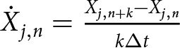 ${\dot X_{j,n}} = \frac{{{X_{j,n + k}} - {X_{j,n}}}}{{k\Delta t}}$, where Δt is the time step (1 month in this study) and k ≥ 1 (integer). To calculate the reverse information flow ${T_{1 \to 2}}$, one simply interchanges the indices 1 and 2 in the formula, with the unit being nats (natural units of information) per unit time. The information flow formulation can also be expressed in terms of linear correlation coefficients and the normalized derivative-covariances, as detailed by Liang (Reference Liang2014), leading to the important implication that, in linear systems, causality necessarily implies correlation, but correlation does not necessarily imply causality (Liang, Reference Liang2016). Although derived under a linear approximation, the estimator has been shown to perform robustly in nonlinear systems (Liang, Reference Liang2014).
A unique property of information flow measure is its asymmetry between the two directions,  ${T_{2 \to 1}}$ and ${T_{1 \to 2}}$, together with the principle of nil causality, which states that if the evolution of one variable is independent of another, the corresponding information flow must be zero. Specifically, if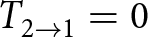 ${T_{2 \to 1}} = 0$, then ${X_2}$ has no causal effect on ${X_1}$, if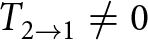 ${T_{2 \to 1}} \ne 0$, a causal relationship exists from ${X_2}$ to ${X_1}$: a positive ${T_{2 \to 1}}$ means that variability in ${X_2}$ contributes to increasing the entropy of ${X_1}$, while a negative value indicates that ${X_2}$ functions to reduce the entropy of ${X_1}$. Statistical significance testing must be employed to verify whether ${T_{2 \to 1}}$ is significantly different from zero.
To eliminate the influence of numerical scale differences between variables, Liang introduced a normalized information flow formula (Liang, Reference Liang2015):
 \begin{equation}\begin{array}{*{20}{c}}
{{\tau _{2 \to 1}} = \frac{{{T_{2 \to 1}}}}{{\left| {{T_{2 \to 1}}} \right| + \left| {\frac{{dH_1^{\text{*}}}}{{dt}}} \right| + \left| {\frac{{dH_1^{{\text{noise}}}}}{{dt}}} \right|}}}
\end{array}\end{equation}
\begin{equation}\begin{array}{*{20}{c}}
{{\tau _{2 \to 1}} = \frac{{{T_{2 \to 1}}}}{{\left| {{T_{2 \to 1}}} \right| + \left| {\frac{{dH_1^{\text{*}}}}{{dt}}} \right| + \left| {\frac{{dH_1^{{\text{noise}}}}}{{dt}}} \right|}}}
\end{array}\end{equation}where  $\frac{{dH_1^{\text{*}}}}{{dt}}$ represents the contribution of system dynamics to entropy, describing how the dynamic changes of the system in phase space affect the uncertainty of variable ${X_1}$. This originates from the intrinsic dynamical properties of the system, such as how the state of ${X_1}$ evolves over time. Correspondingly, $\frac{{dH_1^{{\text{noise}}}}}{{dt}}$ represents the influence of noise on the uncertainty of ${X_1}$. The noise contribution increases the marginal entropy of ${X_1}$, thereby making τ more conservative under noisy conditions. Under the linear approximation used for time-series estimation, these two terms are estimated directly from the same covariance-based statistics used to estimate ${T_{2 \to 1}}$. The core concept of the normalized information flow formulation is to compare the information flow strength ${T_{2 \to 1}}$ with the other contributions to the entropy change of ${X_1}$ (represented by $\frac{{dH_1^{\text{*}}}}{{dt}}$ and $\frac{{dH_1^{{\text{noise}}}}}{{dt}}$), thereby obtaining the normalized information flow strength ${\tau _{2 \to 1}}$. Consequently, the results are no longer affected by the scale of the variables themselves, ensuring good comparability between different datasets.
A statistically significant 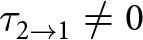 ${\tau _{2 \to 1}} \ne 0$ indicates causal influence from ${X_2}$ to ${X_1}$, whereas ${\tau _{2 \to 1}}$= 0 implies no causality. In this study, we focus on the absolute value of ${\tau _{2 \to 1}}$, expressed as a percentage, to quantify the causal strength representing the magnitude of influence of ${X_2}$ on ${X_1}$.
3.3. Significant test
The statistical significance of information flow  $\tau $ was evaluated through a nonparametric bootstrap procedure (Docquier and others, Reference Docquier2024). For each causal pair, 1000 bootstrap iterations were generated by resampling the original time series with replacement while preserving the original temporal length. For each iteration, the rate of information flow $\tau $ was recomputed by recalculating all terms involved in Eqs (2) and (3) based on the resampled data. The uncertainty of $\tau $, denoted as ${ \in _\tau }$, was quantified as the standard deviation across the 1000 bootstrap estimates. Statistical significance testing was performed by constructing 95% confidence intervals ( $\tau \pm 1.96{ \in _\tau }$). Causal relationships were considered statistically significant at $\alpha = 0.05$ when the confidence interval excludes zero. Pairs whose 95% confidence interval includes zero are treated as noncausal in this dataset (i.e. τ is indistinguishable from zero given the available record length and noise level).
3.4. Multiple linear regression (MLR) model
To complement and validate the causal relationships revealed by the LKIF causal analysis, we employed an MLR model using frontal ablation as the dependent variable to quantify the statistical contributions of drivers. Details of the frontal ablation calculation are provided in Section 2.2. The analysis proceeded through the following steps.
i. The explanatory variables were selected based on the LKIF results, prioritizing those with stronger causal impacts on frontal ablation. To avoid multicollinearity among them, one from any highly correlated pair representing a similar physical process was excluded, ensuring that each final regressor represented a distinct physical process.
ii. Given the inherent memory in glacier–climate systems, each predictor was tested for temporal autocorrelation. We incorporated a temporal lag for each predictor to account for delayed responses of frontal ablation to climate forcing.
iii. Potential outliers were identified using Bonferroni-adjusted p values and subsequently removed. The Bonferroni adjustment (Bland and Altman, Reference Bland and Altman1995) corrects for multiple comparisons by dividing the significance threshold by the number of simultaneous tests conducted on the dataset.
iv. The Lindeman, Merenda and Gold (LMG) method (Lindeman and others, Reference Lindeman, Merenda and Gold1980) was applied to assess the relative importance of each predictor in explaining the variability of frontal ablation within the final MLR model. The LMG method quantifies a predictor’s relative importance by averaging its marginal contribution to R 2 over all possible orderings of variables. This process yields a robust attribution that accounts for inter-predictor correlations. The LMG (Grömping, Reference Grömping2006) can be defined as follows:
 \begin{equation}\begin{array}{*{20}{c}}
{LMG\left( {{x_k}} \right) = \frac{1}{{p!}}{\sum }_{r{\text{ permutation}}} seq{\text{ }}{R^2}\left( {\left\{ {{x_k}} \right\}{\text{|}}r} \right){\text{ }}}
\end{array}\end{equation}
\begin{equation}\begin{array}{*{20}{c}}
{LMG\left( {{x_k}} \right) = \frac{1}{{p!}}{\sum }_{r{\text{ permutation}}} seq{\text{ }}{R^2}\left( {\left\{ {{x_k}} \right\}{\text{|}}r} \right){\text{ }}}
\end{array}\end{equation}where seq R 2 denotes sequential R 2. ‘Sequential’ means that the regressors are entered into the model in the order they are listed. The additional R 2 when adding a regressor xk to a model with the regressors in set Sk(r) is given as  $seq\,R^{2}(\{x_{k} \}{\text{|}}S_{k}(r)) = R^{2}(\{x_{k}\}\,\cup\,S_{k}(r)) - R^{2}(S_{k}(r))$ and the coefficient of determination R 2 can be written as modeled sums of squares (SS) by the total SS: ${R^2}\left( S \right) = \frac{{{\text{Model SS}}\left( {{\text{model with regressors in set }}S} \right)}}{{{\text{Total SS}}}}$. Orders with the same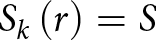 ${S_k}\left( r \right) = S$ can be summarized into one summand, allowing Eqn (4) to be rewritten as
 \begin{align}\begin{array}{*{20}{c}}
LMG\left( {{x_k}} \right) = \frac{1}{{p!}} \sum_{S \subset \left\{ {{x_1} \ldots {x_p}} \right\}\backslash \left\{ {{x_k}} \right\}} \nonumber \\
n\left( S \right)!\left( {p \!-\! n\left( S \right) \!-\! 1} \right)!seq{\text{ }}{R^2}\left( {\left\{ {{x_k}} \right\}{\text{|}}S} \right){\text{ }}
\end{array}\end{align}
\begin{align}\begin{array}{*{20}{c}}
LMG\left( {{x_k}} \right) = \frac{1}{{p!}} \sum_{S \subset \left\{ {{x_1} \ldots {x_p}} \right\}\backslash \left\{ {{x_k}} \right\}} \nonumber \\
n\left( S \right)!\left( {p \!-\! n\left( S \right) \!-\! 1} \right)!seq{\text{ }}{R^2}\left( {\left\{ {{x_k}} \right\}{\text{|}}S} \right){\text{ }}
\end{array}\end{align} Here,  $p$ is the total number of regressors in the final model, and $n\left( S \right)$ denotes the number of regressors in set $S$. This formula shows that LMG is the average over average contributions in models of different sizes.
4. Results
4.1. Changes of the three major glaciers from 2000 to 2021
The terminus positions of JI, KG and HG exhibit sustained long-term retreat between 2000 and 2021, but with notable differences in retreat magnitude and timing (Figs 2–4). All three glaciers show clear seasonal cycles—advancing during winter and retreating in summer (Figs 5–7).
JI experienced a cumulative retreat of ∼20 km (Fig. 2a), with pronounced seasonal variability. Following a transition onto a retrograde slope after 2003 (Fig. 2c), the glacier’s maximum summer terminus position retreated almost every year through 2011. Major retreat events were recorded in 2003 and 2009, coinciding with the disintegration of its long-term floating tongue and elevated summer runoff, respectively. Ice velocity peaked in 2012–13 (Fig. 5b), while from 2012 to 2016, the extent of maximum summer retreat remained consistent. Following this period, stable winter advances for three subsequent years temporarily slowed the net retreat, likely associated with a sustained temperature drop at 250 m depth (Fig. 5d), before the retreat trend appeared to resume around 2020.
Over two decades, KG experienced ∼10 km of retreat (Fig. 3a), marked by a significant retreat in 2005 followed by a period of relative stability until 2016. Anomalous retreat occurred during the winters of 2016 and 2017, attributed by Bevan and others (Reference Bevan, Luckman, Benn, Cowton and Todd2019) to elevated polar surface temperatures that reduced mélange buttressing. This mechanism is corroborated by Fig. 6d, which shows warmer ocean surface conditions in 2016 and 2017 relative to the preceding years. Unlike the JI glacier, KG displays a ∼3 month phase lag in its seasonal cycle, with peak retreat occurring in November–December and peak advance in June. Topographically, KG is situated on a low-gradient retrograde slope (Fig. 3c and d), where further inland retreat could amplify instability through positive feedback mechanisms (Felikson and others, Reference Felikson2017).
HG followed a different topographic evolution from the other two glaciers, retreating from a retrograde slope (2000–03) onto a prograde bed (2004–21), with a pinning feature ∼15–20 km inland (Fig. 4c and d). Compared to the other two glaciers, HG’s terminus was generally more stable, with a less pronounced seasonal cycle. Despite this relative stability, it experienced a major, rapid retreat in 2005, coinciding with a significant increase in runoff and low SIC, followed by a subsequent re-advance and stabilization from 2006 to 2015. Then its terminus retreated further inland than its 2005 position in 2017 and 2019. Notably, these major retreat phases coincided with ocean surface warming and SIC decrease (Fig. 7), implying a more fragile state that is highly vulnerable to oceanic forcing.
4.2. LKIF between glacier terminus position and environmental forcing
Glacier terminus retreat phases for JI and HG typically align with runoff periods, concurrently characterized by reduced SIC, elevated ocean thermal forcing at 5 m (OTF5m) and 250 m (OTF250m) and air temperatures (T A) (Figs 5 and 7). Furthermore, subglacial bed slope appears to modulate glacier terminus behavior, though this relationship is ambiguous. These qualitative spatiotemporal associations, while suggestive, do not constitute evidence of direct causal mechanisms nor reliably identify the dominant drivers of glacial change.
To rigorously identify directional causal mechanisms, we applied the LKIF method to quantify information transfer from potential climatic and oceanic forcing factors to GTPC for JI, KG and HG during 2000–21. Due to its binary (presence/absence) nature and limited temporal availability, ice mélange data were excluded from the LKIF analysis, as discrete variables are incompatible with information-theoretic approaches that require continuous distributions for reliable causal inference. The resulting causal relationships were subsequently compared with traditional Pearson correlation analyses to evaluate method consistency and identify potential discrepancies between correlation-based and causality-based approaches (Fig. 8). For this comparative analysis, time lags were varied from zero to 3 months to allow for a delayed response of glacier terminus position to external forcing factors.
Absolute rates of information transfer (|τ|) from bed slope, sea-ice concentration (SIC), air temperature (T A), runoff, ocean thermal forcing (OTF) at 5 and 250 m depth to GTPC for the three glaciers during 2000–21 (left panels) and Pearson correlation coefficients between them (right panels) with no time lag (the 1st row), 1 month lag (the 2nd row), 2 month lag (the 3rd row) and 3 month lag (the 4th row). Colored circles represent values for individual glaciers, with black outlines indicating statistical significance at the 95% confidence level.

Figure 8 Long description
Lag 0: The tau plot shows information transfer from Bed slope, SIC, Runoff, T, OTF5m and OTF250m. Values range from 0 to 20 percent, with notable peaks at SIC and Runoff. The R plot shows correlation coefficients ranging from negative 1 to 1, with SIC showing negative correlation and Runoff showing positive correlation. Lag 1: The tau plot shows increased values for Runoff and T, peaking at 18 percent. The R plot shows mixed correlations, with Runoff and T having positive values. Lag 2: The tau plot shows moderate values, with T peaking at 16 percent. The R plot shows mostly negative correlations, except for T. Lag 3: The tau plot shows higher values for SIC and T, peaking at 18 percent. The R plot shows mixed correlations, with SIC and T having positive values. The legend distinguishes datasets by colors: JI, KG, HG. Higher tau does not consistently align with stronger correlations, indicating different insights from each metric.
The Pearson correlation analysis revealed that bed slope has little to no meaningful association with GTPC across all time lags (0–3 months), with only an isolated significant correlation (Fig. 8b and h). Consistently, the causal analysis detects no significant causality between bed slope and GTPC at any lag (Fig. 8).
The three glaciers demonstrated consistent causal relationships and Pearson correlation patterns between GTPC and both runoff and near-surface air temperature (Fig. 8), as runoff is largely temperature-driven. Pearson correlation analysis generally supports these relationships, although lagged correlations are more sensitive to seasonal phase shifts and may change sign at longer lags.
Correlation analysis and causality analysis reveal detectable but moderate relationships from SIC to GTPC. For KG, SIC and GTPC show significant causality and negative correlations at 0 month lag (R = −0.51). For JI and HG, the information transfer from SIC to GTPC and their correlation are weaker than KG and only significant at specific lags. It is well understood that correlation can sometimes be misleading about causation.
For ocean thermal forcing at 5 m, KG exhibits both positive correlations and causal relationships at short time lags (0–1 month). For HG, causality emerges mainly at longer lags (1–3 months). For JI, information transfer from OTF5m to GTPC is significant at all lags, peaking at 2 month lag. Overall, KG responds rapidly to OTF5m, whereas JI and HG exhibit a multi-month delayed response. For OTF250m, the inferred causal influence is generally comparable to, or lower than, that of OTF5m.
For KG, while a causal relationship from runoff to GTPC is evident at short lags and weakens as the lag increases (Fig. 8), the correlation remains positive across all lags. For JI, information transfer from runoff to GTPC is significant at all lags and progressively increases. For HG, information transfer appears at 2–3 months. For JI and HG, positive correlations consistent with runoff-enhanced retreat are observed only at lag 0; at longer lags, the correlations become negative, likely reflecting seasonal phase shifts.
To consider seasonal variations in glacier termini responses, we carried out season-specific analyses by categorizing the forcing data into two periods: summer (from May to October) and winter (from November to April) (Fig. 9). For a 3 month lag, forcing values from the summer subset (May–October) are therefore paired with GTPC observed 3 months later, covering August–January. Accordingly, the seasonal interpretation becomes less strictly seasonal at longer lags, but it still provides a useful basis for assessing seasonal variability in the sensitivity of GTPC to external forcing.
Seasonal contrast in absolute rates of information transfer (|τ|) from bed slope, sea-ice concentration (SIC), runoff, air temperature (T A) and ocean thermal forcing (OTF) at 5 and 250 m depth to GTPC for three major glaciers during 2000–21. Left panels: Summer regime (May–October); Right panels: Winter regime (November–April). Colored circles represent values for individual glaciers, with black outlines indicating statistical significance at the 95% confidence level.

Figure 9 Long description
The image consists of eight scatter plots arranged in two columns, representing seasonal contrasts in information transfer rates from various environmental factors to glacier termini position changes. The left column shows summer regimes (May-October) and the right column shows winter regimes (November-April). Each row corresponds to a different lag period from 0 to 3. The horizontal axis in each plot represents different environmental factors: Bed Slope, Sea Ice Concentration (SIC), Runoff, Air Temperature (T), Ocean Thermal Forcing at 5 meters (OTF5m) and Ocean Thermal Forcing at 250 meters (OTF250m). The vertical axis represents the information transfer rate in percentage. Colored circles indicate values for individual glaciers, with red, blue and yellow representing different glaciers. Black outlines around some circles indicate statistical significance at the 95 percent confidence level. In the summer regime, higher information transfer rates are observed for Bed Slope and Air Temperature, especially at Lag 0. In the winter regime, Sea Ice Concentration and Ocean Thermal Forcing at 5 meters show notable values. The plots illustrate seasonal variability in glacier sensitivity to these factors, with some clusters and outliers visible, particularly in the summer plots.
We quantify the seasonal partitioning of terminus movement (Supplementary Fig. S3). During the runoff season, over 70–80% of total retreat occurred across all three glaciers. In contrast, during winter when ice mélange was present, JI and KG exhibited substantial seasonal advance (∼60% of total change), while HG showed only modest forward motion (∼50%). These contrasts reflect glacier-specific sensitivities to seasonal forcings, probably largely due to the prograde bedrock beneath the HG terminus.
During summer, surface air temperature ( ${T_{\text{A}}}$) and runoff emerge as the primary immediate drivers of terminus position variations for JI and KG at 0 month lag and for HG at 2 month lag. OTF5m maintains high information transfer levels for JI at lags of 0–2 months and for HG at 1 month lag, highlighting sustained causal effects likely driven by prolonged oceanic heat exchange at the glacier terminus. For JI and KG, SIC affects GTPC in the same month. For HG, SIC only affects GTPC with a time lag of 1 month. We speculate that this time lag represents the consolidation period required for newly formed sea ice to cement calved icebergs into a mélange rigid enough to inhibit calving and stabilize the terminus.
Information transfer from most external forcing is much lower during winter than summer, with many flows falling below the statistical significance threshold for the three glaciers. This substantial seasonal difference indicates weaker detectable influences of external forcings during winter in the monthly lagged analysis, consistent with diminished runoff, lower temperatures and relatively stable oceanic conditions, leading to limited dynamic glacier terminus responses. However, it is noteworthy that during winter, SIC continued to exert significant immediate influence on JI and KG and is the clearest forcing signal among the variables considered for winter terminus stability (Fig. 9). In winter, the fjord in front of JI and KG is filled with ice mélange (Bevan and others, Reference Bevan, Luckman, Benn, Cowton and Todd2019; Joughin and others, Reference Joughin, Shean, Smith and Floricioiu2020), and SIC may influence GTPC by providing favorable conditions for ice mélange formation and persistence within the fjord. OTF5m also shows detectable information transfer to GTPC for JI and KG, possibly reflecting the influence of near-surface ocean conditions on sea ice and mélange development.
Seasonal analysis reveals that the dominant information transfers identified at the annual scale—particularly from runoff and thermal forcings—are largely driven by summer conditions, while winter contributions are less evident in the present analysis. Furthermore, the estimated bed slope near the terminus shows consistently weak information transfer at all time lags studied, indicating that this local slope metric alone serves as a weak proxy for the broader influence of subglacial topography on terminus dynamics.
4.3. The effect of ocean thermal forcing on glacier terminus position varies with water depth
We analyzed the causal relationship between OTF at different depths and GTPC. Figure 10 demonstrates that the causal impact of OTF on GTPC is concentrated in the depth range where each glacier appears most responsive to ocean heat, producing a coherent but glacier-specific pattern.
Depth-dependent information transfer from ocean thermal forcing (OTF) to GTPC. The profiles show the absolute information transfer ( $\left| \tau \right|$) as a function of depth (0–500 m) for JI, KG and HG at monthly lags 0–3. Red circles indicate statistical significance at the 95% confidence level.

Figure 10 Long description
The image consists of twelve scatter plots arranged in a grid, showing depth-dependent information transfer from Ocean Thermal Forcing to GTPC. The x-axis is labeled ′Information transfer |T|′ in percent, ranging from 0 to 25. The y-axis is labeled ′Depth′ in meters, ranging from 0 to 500. Each column represents a different glacier: JI, KG and HG. Each row corresponds to a different monthly lag: 0, 1, 2 and 3. Red circles indicate statistical significance at the 95 percent confidence level, while blue circles represent non-significant data points. For JI, at lag 0, significant information transfer is concentrated at shallow depths, decreasing with depth. At lag 1, significant points appear at mid-depths. At lag 2, significant points are scattered throughout and at lag 3, they are concentrated at shallow depths again. For KG, at lag 0, significant points are concentrated at shallow depths. At lag 1, they appear at mid-depths. At lag 2, significant points are scattered and at lag 3, they are concentrated at shallow depths. For HG, at lag 0, significant points are concentrated at shallow depths. At lag 1, they appear at mid-depths. At lag 2, significant points are scattered and at lag 3, they are concentrated at shallow depths. The plots illustrate how the causal impact of Ocean Thermal Forcing on GTPC varies by glacier and lag, with significant effects often occurring at shallower depths.
JI exhibits strong information transfer from OTF to GTPC in the upper ∼100 m at time lags of 0–3 months, with |τ| value peaking at ∼17% at 2 month lag. Below 100 m, weaker but significant information transfer is detected at 3 month lag, consistent with the causal relationships from OTF250m to GTPC at 3 month lag for JI (Fig. 8). It is likely due to the presence of a shallow sill (∼265 m) at the fjord mouth, which restricts deep water inflow and limits deep ocean influence.
KG shows significant information flow mainly at 0 month lag, with a pronounced signal extending through much of the upper ∼400 m; at this time,  $\left| \tau \right|$ peaks near the surface (15%) and progressively weakens with depth. This broad vertical reach likely reflects efficient shelf-fjord connectivity, which allows ocean thermal forcing across the water column to penetrate the fjord and influence the terminus. At 1 month lag, only weakly significant information transfer remains near the surface, while no significant signal is detected at 2 month lag. By a 3 month lag, the signal reappears but remains weak and is mainly confined to the 70–200 m layer.
The influence of OTF on HG is weak, with significant causality appearing at lags of 0–2 months across most of the vertical profile. Although Atlantic water occupies in Sermilik Fjord where HG terminates, its heat transport is about ten times lower than in Kangerdlugssuaq Fjord where KG terminates due to much smaller Atlantic water volume inflow (Inall and others, Reference Inall2014). Limited heat supply, strong surface stratification and a prograde bed slope together constrain its impact on terminus retreat.
4.4. Parameterizing frontal ablation using climatic and oceanic forcings
Although our primary causal analysis in preceding sections focused on GTPC, a parallel analysis using frontal ablation as the response variable revealed highly consistent information transfer patterns (see Supplementary Figs S4–S6). The causal structure of the drivers and their seasonal dependencies’ responses to OTF closely mirrored those of GTPC and are therefore not repeated here.
Building upon the causal results, we further parameterized frontal ablation to provide a quantitative representation of calving processes. LKIF was used to identify causally supported drivers, and an MLR model was used as a simple and operable first-order representation of frontal ablation. The relative importance of predictors was assessed using the LMG method.
For frontal ablation parameterization, we selected runoff, SIC and OTF5m. Subglacial runoff was used because it stimulates buoyant upwelling adjacent to the terminus (Jenkins, Reference Jenkins2011) and drives the renewal of warm water in the fjord (Cowton and others, Reference Cowton, Sole, Nienow, Slater and Christoffersen2018). SIC represents mélange buttressing, while OTF5m was selected because it exhibits the strongest information flow across time lags (Fig. 10), capturing surface-layer thermal forcing that can weaken mélange.
We assume that frontal ablation, FA, at time t can be expressed by a multi-additive model incorporating both concurrent and lagged effects of the forcings:
 \begin{align}
F{A_t} & = C + \mathop \sum \limits_{i = 0}^3 {\alpha _i}\cdot\left( {1 - SI{C_{t - i}}} \right) + \mathop \sum \limits_{i = 0}^3 {\beta _i}\cdot{Runof}{f_{t - i}} \nonumber\\
& \qquad + \mathop \sum \limits_{i = 0}^3 {\gamma _i}\cdot{OT}{F_{5m,{\text{ }}t - i}}
\end{align}
\begin{align}
F{A_t} & = C + \mathop \sum \limits_{i = 0}^3 {\alpha _i}\cdot\left( {1 - SI{C_{t - i}}} \right) + \mathop \sum \limits_{i = 0}^3 {\beta _i}\cdot{Runof}{f_{t - i}} \nonumber\\
& \qquad + \mathop \sum \limits_{i = 0}^3 {\gamma _i}\cdot{OT}{F_{5m,{\text{ }}t - i}}
\end{align}where  $C$ is a constant, i denotes the time lag and ${\alpha _i}$, ${\beta _i}$, ${\gamma _i}$ represent the sensitivities of FA to SIC, Runoff and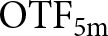 ${\text{OT}}{{\text{F}}_{5{\text{m}}}}$ at lag i, respectively.
The model results (Fig. 11) are consistent with the causal inference findings (Fig. 8). The selected drivers collectively explain 66.3% of frontal ablation variance for JI, 53.2% for KG and 38.5% for HG, confirming HG’s lower sensitivity to climatic forcings. OTF₅m dominates frontal ablation variability for JI (50.7% of the explained variance), whereas runoff is the leading driver for KG and HG (46.1% and 45.2%, respectively), indicating that frontal ablation is primarily governed by oceanic and atmospheric forcing, with SIC contributing only secondarily.
Relative importance of drivers explaining frontal ablation (FA) variance for JI, KG and HG. Bars show the percentage contribution of OTF₅m, SIC and runoff to the total explained variance (R 2), calculated via the LMG method. Total R 2 for each glacier is noted above each panel.

A time-lagged decomposition (Fig. 12) reveals contrasting glacier response behaviors. KG exhibits a rapid response to atmospheric forcing, with the relative importance of runoff peaking at lag 0 (20.9%) and remaining high at lag 1 (15.8%). In contrast, JI shows a more delayed and persistent response dominated by oceanic forcing, with the importance of OTF5m remaining significant across lags 0–3 and peaking at lag 2 (17.4%). Runoff and SIC also show sustained contributions to the frontal ablation of JI. For HG, the model explains the least variance, and runoff contributes the most, reflecting HG’s limited sensitivity to external climatic forcing. Overall, the relative importance patterns of these climatic drivers are broadly consistent with the LKIF results, reinforcing the robustness of the inferred glacier–climate linkages.
Time-labeled relative importance of drivers explaining frontal ablation (FA) variance for JI, KG and HG. Plots disaggregate the total importance from Figure 11, showing the percentage contribution of each variable to the total R 2 at monthly lags of 0–3 months.

Figure 12 Long description
Three grouped bar graphs titled JI, KG and HG. JI: Vertical axis label Relative importance percent of R superscript 2. Horizontal axis labels lag0, lag1, lag2, lag3. Legend entries OTF5m, SIC, Runoff. Values at lag0: OTF5m 4.1 percent, SIC 10.8 percent, Runoff 4.1 percent. Values at lag1: OTF5m 12.7 percent, SIC 5.9 percent, Runoff 4.2 percent. Values at lag2: OTF5m 17.4 percent, SIC 4.6 percent, Runoff 6.9 percent. Values at lag3: OTF5m 16.5 percent, SIC 3.4 percent, Runoff 9.4 percent. KG: Vertical axis label Relative importance percent of R superscript 2. Horizontal axis labels lag0, lag1, lag2, lag3. Legend entries OTF5m, SIC, Runoff. Values at lag0: OTF5m 17.9 percent, SIC 9.7 percent, Runoff 20.9 percent. Values at lag1: OTF5m 10.7 percent, SIC 5.0 percent, Runoff 15.8 percent. Values at lag2: OTF5m 4.3 percent, SIC 2.3 percent, Runoff 6.9 percent. Values at lag3: OTF5m 1.8 percent, SIC 2.2 percent, Runoff 2.5 percent. HG: Vertical axis label Relative importance percent of R superscript 2. Horizontal axis labels lag0, lag1, lag2, lag3. Legend entries OTF5m, SIC, Runoff. Values at lag0: OTF5m 6.3 percent, SIC 2.5 percent, Runoff 15.4 percent. Values at lag1: OTF5m 5.0 percent, SIC 6.2 percent, Runoff 4.5 percent. Values at lag2: OTF5m 10.3 percent, SIC 9.0 percent, Runoff 4.6 percent. Values at lag3: OTF5m 8.9 percent, SIC 6.7 percent, Runoff 20.8 percent.
5. Discussion
5.1. Causal mechanisms revealed by LKIF
We employed a causal analysis method, LKIF and characterized the primary drivers of GTPC and frontal ablation for three major outlet glaciers—JI, KG and HG. The results indicate that SIC, runoff,  ${T_{\text{A}}}$ and OTF5m all exert notable influences on glacier dynamics, with atmospheric forcing proving to be nearly as important as oceanic forcing. Distinguishing causality from correlation is critical; our results show that some lagged correlations change sign, likely due to seasonal phase shifts, whereas LKIF provides a more stable measure of directional information transfer. While all three glaciers exhibited significant causal linkages to external forcings, their sensitivities differed in both magnitude and type. JI shows a relatively balanced overall response to both atmospheric and oceanic drivers, consistent with its exposure to warm waters. KG responded more acutely to short-term runoff events, with causal strength peaking at shorter lags—indicating a rapid dynamic feedback, possibly due to unstable winter mélange and the proximity of large overdeepened reverse slopes, where mélange loss rapidly amplifies melt-driven retreat (Barnett and others, Reference Barnett, Holmes and Kirchner2023). HG exhibited the weakest overall causal signals and the most muted terminus fluctuations, suggesting greater dynamic stability and perhaps stronger topographic control from its prograde bed slope. These differences likely reflect a combination of subglacial runoff, fjord geometry, ice mélange persistence and bed topography, which modulate how external forcings translate into glacier dynamical change.
Despite the persistent long-term retreat observed in all three glaciers over the past two decades, their terminus positions still exhibit a strong seasonal cycle—retreating in summer and advancing or stabilizing during winter (Figs 5–7). In summer, elevated air temperatures enhance surface meltwater production and reduce sea-ice formation, while winter mélange stabilizes the terminus through winter mélange-associated backstresses. Driven by these seasonal climate forcings, the terminus stress regime shifts fundamentally, thereby modulating the glacier’s sensitivity to external drivers (Greene and others, Reference Greene, Gardner, Wood and Cuzzone2024). Based on this, we decomposed the data seasonally and performed separate information flow analyses. The results revealed that the strength of causal information flow from external forcings also varies with season. In summer, atmospheric drivers such as  ${T_{\text{A}}}$ and runoff show clear influences on GTPC across all three glaciers. Elevated air temperatures drive higher surface melt rates, and the resulting runoff may promote hydrofracturing (van der Veen, Reference van der Veen1998) and basal lubrication (Zwally and others, Reference Zwally2002), which could elevate ice flow and potentially weaken terminus integrity. For example, fresh meltwater routed to the glacier base may power buoyant subglacial plumes that entrain warm fjord water and undercut the ice front, potentially triggering calving (van der Veen, Reference van der Veen1998; O’Leary and Christoffersen, Reference O’Leary and Christoffersen2013). In addition, warm air and increased surface melt may reduce ice tensile strength and promote crevassing, preconditioning the terminus for failure.
In contrast, the winter-season analysis revealed that the causal influence of most external forcings on GTPC became insignificant. During winter, the lack of surface meltwater input may lead to reduced subglacial hydrological activity, which could weaken the coupling between atmospheric forcing and glacier dynamics. Consequently,  ${T_{\text{A}}}$ and runoff might not effectively accelerate ice flow or trigger terminus change. SIC and OTF5m still retain some winter influence, likely reflecting the role of sea-ice conditions and near-surface ocean heat in regulating mélange development. In this context, the mélange—composed of sea ice, icebergs and calved ice fragments—remains largely intact and persistent throughout winter. The mélange acts as a mechanical buttress that resists calving and stabilizes the glacier front (Amundson and others, Reference Amundson2010). Consequently, the absence of effective atmospheric and oceanic perturbations in winter leads to a marked reduction in the strength of LKIF to the GTPC.
5.2. Surface-layer dominance in ocean thermal forcing
Our analysis indicates that the causal influence of ocean thermal forcing on GTPC and frontal ablation appears most pronounced in the upper 0–100 m of the ocean surface layer for JI and KG (Fig. 10). While submarine melting is typically associated with warm Atlantic Water at depth (Cowton and others, Reference Cowton, Sole, Nienow, Slater and Christoffersen2018), the inferred information flow in deeper layers exhibits lower intensity.
One plausible explanation is that the glacier’s response to oceanic heat forcing is often mediated by surface-layer processes. A prominent example is the role of mélange. When surface ocean temperatures are anomalously warm, the formation of sea ice is suppressed, reducing the mechanical stability of mélange. This weakened mélange fails to provide sufficient back stress, exposing the glacier front to the open ocean and triggering increased calving and terminus retreat. For instance, KG experienced anomalously warm winters during 2016–18, during which the unstable mélange formation was associated with a lack of seasonal advance and persistent multi-year retreat (Bevan and others, Reference Bevan, Luckman, Benn, Cowton and Todd2019). These observations highlight that surface water may exert indirect yet significant influence by modulating the stability of fjord mélange.
Although Atlantic water below 200 m is theoretically expected to drive substantial basal melt, our information flow analysis indicates only a weak causal influence of deep water on terminus variations. This absence may partly reflect data limitations: our ocean temperature fields were derived from reanalysis data at offshore coastal grid points near, but not within, the fjords, and thus may not fully capture the fjord-specific vertical thermal structure. Furthermore, shallow sills at the fjord mouths of JI likely restrict the inflow of deep warm water, which would further dampen the transmission of deep-ocean causal signals to the glacier termini. Even so, the finding of no significant information flow, despite potential observational bias, lends weight to the interpretation that deep warm water plays a more limited role in controlling terminus variability. This is consistent with process-based evidence: previous numerical modeling has shown that even under relatively high melt rates, frontal melting alone can only induce limited terminus retreat and has little influence on multiannual mass balance (Barnett and others, Reference Barnett, Holmes and Kirchner2023). In fast-flowing tidewater glaciers, terminus changes are primarily governed by high-frequency calving events and variations in upper-layer ocean temperature, with ice loss from calving often exceeding that from submarine melting (Krug and others, Reference Krug, Durand, Gagliardini and Weiss2015). Barnett and others (Reference Barnett, Holmes and Kirchner2023) further showed that for KG, increased submarine melt—whether from deep Atlantic water inflow or runoff—had little effect unless winter mélange buttressing was lost, in which case retreat into over-deepened reverse slopes greatly amplified melt-driven retreat. Furthermore, the geoengineering intervention experiments for JI in which ‘curtains’ blocking deep warm water inflow reduced fjord temperatures but produced only minor changes in retreat trajectories and failed to prevent continued retreat once MISI had been initiated (Zhao and others, Reference Zhao, Luo, Wolovick, Mettiäinen and Moore2025). These results suggest that deep warm water may play a more limited role in controlling terminus retreat than expected, and that similar deep-water blocking measures are unlikely to be effective for other rapidly retreating marine-terminating outlets in Greenland that have already passed critical stability thresholds.
At the same time, a glacier’s sensitivity to thermal forcing, particularly submarine melting, depends strongly on its instantaneous terminus position, grounding state and bed geometry (Barnett and others, Reference Barnett, Holmes and Kirchner2023). Thus, submarine melting likely assumes a dominant role only during specific unstable phases, such as when retreat onto reverse-sloping bedrock increases the submerged ice-ocean contact area, thereby amplifying the glacier’s response to thermal forcing. However, over the two-decade analysis period considered here, such unstable configurations may not have persisted continuously, which could partly explain the weak causal linkage detected between submarine melting and terminus position in our results. In glacier-ocean systems, the effectiveness of external forcing is constrained by geometry and environmental setting. Ocean thermal forcing can affect terminus dynamics only if warm subsurface waters reach the glacier front, which is limited by fjord bathymetry and sill geometry. Causal relationships from a given forcing are thus valid only under the geometric and dynamical conditions of the analyzed period. When a glacier retreats into a substantially different configuration, the relative importance of forcings may change, as seen in the three glaciers studied. Our information flow analysis therefore focuses on periods where large-scale geometric conditions remain stable. This also implies that, when applying the information-flow approach to other glaciers, inferred causal links should be interpreted as conditional on the local geometric setting and are likely to be most consistent when the glacier remains within a broadly similar bed/fjord configuration (i.e. without major long-term geometric changes). If large geometric changes occur, the relative importance and apparent causal pathways of external forcings may shift, and the causality should be reassessed for the new setting. The validity of information-flow causal inference depends on whether the time series sufficiently samples a statistically stable dynamical regime, rather than a fixed physical length. Short time series may increase uncertainty, while adequate sampling recovers reliable causal directions.
5.3. The limited causal role of bed slope and the complexity of topographic controls
Despite the fact that classical theory posits that retrograde slopes promote MISI through feedbacks between increased discharge and deepening beds (Weertman, Reference Weertman1974; Schoof, Reference Schoof2007; Fyke and others, Reference Fyke, Sergienko, Löfverström, Price and Lenaerts2018; Catania and Felikson, Reference Catania and Felikson2022), our LKIF results did not identify a significant causal influence of bed slope on glacier terminus variability (Fig. 8). Both JI and KG are situated in such topographic settings (Figs 2 and 3), whereas HG has largely remained on relatively shallow or landward-rising bedrock over the past two decades (Fig. 4). From a purely geometric standpoint, JI and KG should be more prone to MISI-type retreat, while HG appears more stable—a pattern that aligns with our observational data (Figs 5a, 6a and 7a).
However, our LKIF analysis revealed no significant information transfer from bed slope to GTPC (Fig. 8). This finding does not imply that bed topography is irrelevant; rather, it suggests that slope at kilometer-resolution alone is an insufficient predictor in a statistical or causal modeling context. This interpretation is consistent with recent glacial geomorphic reconstructions, which demonstrate that irregular or unmarked retreat is not exclusive to reverse bed slopes but also occurs under complex slope configurations in prograde or variable slope settings (Greenwood and others, Reference Greenwood, Simkins, Winsborrow and Bjarnadóttir2021; Greene and others, Reference Greene, Gardner, Wood and Cuzzone2024). Indeed, the proportion of such retreat styles is broadly similar across slope types, and a notable portion of retreat events on reverse slopes even proceeds in a steady and regular manner.
The influence of bed slope typically manifests only when combined with external forcing (Catania and others, Reference Catania2018). Even glaciers grounded on retrograde slopes may remain stable for extended periods because of buttressing from side walls or complex three-dimensional bed topography unless perturbed by external drivers. It is often the external forcing that triggers the onset of retreat, with bed topography, particularly retrograde slopes, modulating the subsequent rate and extent of grounding-line migration (Seroussi and others, Reference Seroussi2017). For instance, the 2004–05 retreat of KG was precipitated by the collapse of an ice tongue due to ocean warming (Bevan and others, Reference Bevan, Luckman, Benn, Cowton and Todd2019), which resulted in the removal of frontal buttressing and the exposure of a retrograde bed, consequently leading to flow acceleration—a phenomenon that is consistent with MISI. In such cases, bed slope functions more as a post-trigger amplifier than a primary driver, and its static nature limits its detection in time-varying causality frameworks. Recent studies also suggest that once fast ice flow has started, it can continue even in areas where it would not naturally happen (Greenwood and others, Reference Greenwood, Simkins, Winsborrow and Bjarnadóttir2021). In this study, all three glaciers—JI, KG and HG—are fast-flowing outlet glaciers near their termini (Figs 2–4), where sustained high velocities likely diminish the local sensitivity to bed slope.
Another key topographic control is the presence of pinning points, which can temporarily stabilize the terminus by providing basal resistance (Greenwood and others, Reference Greenwood, Simkins, Winsborrow and Bjarnadóttir2021; Williams and others, Reference Williams, Gourmelen, Nienow, Bunce and Slater2021). For instance, the post-2005 stabilization of HG is attributed to its retreat onto a shallow sill at the fjord head. Partially regrounding on this shallower bed likely restored frictional resistance and created a temporary equilibrium (Ekström and others, Reference Ekström, Nettles and Tsai2006). However, such stability is often transient if external warming persists.
It is evident that the intricate interplay of topographic influences on glacier dynamics cannot be fully encapsulated by a solitary one-dimensional scalar slope value. The present findings thus suggest that, while bed topography plays a critical role, it often exerts its influence indirectly and episodically, rather than exerting a direct, continuous influence on GTPC.
5.4. Frontal ablation as a combined response to atmospheric and oceanic forcings
Frontal ablation has accounted for a substantial share of mass loss from the GrIS since the mid-1990s, contributing ∼30–60% of the total annual loss (Shepherd and others, Reference Shepherd2020; Fahrner and others, Reference Fahrner2025). More specifically, a recent study attributed 1034 ± 120 Gt of mass loss between 1985 and 2022 solely to secular glacier terminus retreat (Greene and others, Reference Greene, Gardner, Wood and Cuzzone2024). Yet despite its importance, representing frontal ablation in ice-sheet models remains challenging (Fahrner and others, Reference Fahrner2025).
Building on our quantitative analyses, we parameterized FA using a simple linear regression model with runoff, SIC and OTF5m as predictors. The model reproduces the observed frontal ablation variability well, explaining 66.3%, 53.2% and 38.5% of the variance for JI, KG and HG, respectively, in agreement with the causal inference results. The model’s lower interpretation for HG is likely because Helheim has a lightly grounded terminus, whereas KG has a floating terminus and JI is often near flotation. For glaciers with lightly grounded termini like Helheim, terminus position is the primary control on its dynamics, and the link to climate forcings is indirect (Kehrl and others, Reference Kehrl, Joughin, Shean, Floricioiu and Krieger2017). For glaciers with floating or near-flotation termini like KG and JI, terminus retreat is less coupled to the immediate stress balance, allowing external factors like mélange rigidity and ocean temperature to exert a more direct and detectable influence. Notably, even when the regression is restricted to the top five most influential lagged variables (Supplementary Fig. S7), the explanatory power remains robust (R 2 = 0.560 for JI, 0.501 for KG and 0.356 for HG). This suggests that a limited subset of climatic predictors—primarily runoff and OTF5m—is sufficient to capture the dominant variability in frontal ablation, underscoring the strong climatic control on terminus dynamics.
The relative importance patterns (Figs 11 and 12) indicate that atmospheric warming–induced runoff explains a large fraction of the temporal variability in frontal ablation, particularly for KG, while oceanic thermal forcing exerts a more sustained influence for JI. Meanwhile, SIC provides a secondary but non-negligible control, consistent with its role in modulating mélange buttressing. Together, these findings demonstrate that the retreat of Greenland’s marine-terminating glaciers can be effectively explained as a joint response to atmospheric and oceanic forcings. Rather than being dominated by a single driver, glacier frontal ablation reflects the combined influence of subglacial runoff and ocean thermal conditions, whose interplay governs both the rate and extent of terminus retreat (Cowton and others, Reference Cowton, Sole, Nienow, Slater and Christoffersen2018).
Such a simplified parameterization, linking frontal ablation directly to runoff and ocean temperature, offers a physically grounded yet computationally efficient framework for incorporation into large-scale ice-sheet models. This approach provides a practical means of representing the glacier–climate coupling and improving projections of the GrIS’s response to concurrent atmospheric and oceanic warming.
6. Conclusion
The LKIF method was applied to long-term observations of JI, KG and HG, enabling the quantitative disentangling of the causal drivers of glacier terminus retreat and frontal ablation. Our analysis shows that both atmospheric forcing and oceanic forcing (upper-ocean thermal content) play comparably important roles in driving glacier retreat, particularly during summer. Conversely, the direct effects of winter forcings on terminus position are negligible. Notably, the causal impact of ocean warming is concentrated in the shallow (0–100 m) surface layer of the fjord for JI and KG. Warm surface waters indirectly accelerate retreat by suppressing sea-ice formation and weakening the integrity of the ice mélange, thus exposing the glacier terminus to enhanced calving. In contrast, deep water shows little detectable short-term influence on terminus fluctuations in our analysis. This suggests that, on seasonal to interannual timescales, processes within the surface layer are more critical for glacier front dynamics than submarine melting in deep water. Within this evidence, measures that target deep warm-water inflow—such as ‘curtains’—are unlikely to be decisive once retreat has been initiated: they may reduce fjord temperatures at depth yet leave the mélange–calving pathway largely intact. Static topographic features, such as bed slope, do not appear as direct causal drivers of terminus change on the timescales analyzed. Instead, topography modulates glacier response after external perturbations initiate retreat. In our parameterized frontal ablation model, climate variables (runoff, SIC and upper-ocean thermal forcing) explain about 53–66% of the monthly variability for floating-type glaciers but show weaker explanatory power for lightly grounded glaciers such as Helheim, possibly reflecting the influence of local geometry and terminus position. This confirms that a simple climate-driven model can capture a large fraction of observed calving variability. The application of LKIF provides a rigorous, nonlinear framework for identifying cause-and-effect relationships in the ice–ocean–atmosphere system. Unlike traditional correlation or regression analyses, this method helps distinguish directional causal relationships from spurious associations, providing a more informative basis for interpreting glacier sensitivity. Looking ahead, these findings have important implications for ice-sheet modeling. The identified causal mechanisms point to specific processes that should be represented in simulations: for example, explicit coupling between surface meltwater production, subglacial hydrology and mélange strength, as well as the influence of near-surface ocean warming on glacier fronts. Incorporating these causal pathways into next-generation models will help reduce uncertainty in projections of Greenland’s sea-level contribution.
Supplementary material
The supplementary material for this article can be found at https://doi.org/10.1017/jog.2026.10173.
Data availability statement
TermPicks dataset, Version 2, is available at Zenodo (https://doi.org/10.5281/zenodo.6557981, Goliber and Black, Reference Goliber and Black2021). Data product of Greenland glacier calving front locations delineated by deep learning, 2013 to 2021, is available at https://dx.doi.org/10.25532/OPARA-208 (Loebel and others, Reference Loebel2023). Greenland ice masking is available at https://doi.org/10.5281/zenodo.8388136 (Greene, Reference Greene2023). Greenland Ice Sheet solid ice discharge from 1986 through last month is available at https://doi.org/10.22008/promice/data/ice_discharge (Mankoff and others, Reference Mankoff, Solgaard and Larsen2020). MEaSUREs Greenland Ice Velocity: Selected Glacier Site Velocity Maps from InSAR, version 4, is available at https://doi.org/10.5067/GQZQY2M5507Z (Joughin and others, Reference Joughin, Howat, Smith and Scambos2021). MEaSUREs Greenland 6 and 12 day Ice Sheet Velocity Mosaics from SAR, version 1, is available at https://doi.org/10.5067/6JKYGMOZQFYJ (Joughin, Reference Joughin2021). RACMO2.3p2, statistically downscaled from 5.5 km to 1 km and forced by ERA5 reanalysis, is an extension of Noël and others (Reference Noël, van de Berg, Lhermitte and van den Broeke2019) and is available from the authors upon request. IceBridge BedMachine Greenland, version 5, is available at https://doi.org/10.5067/GMEVBWFLWA7X (Morlighem and others, Reference Morlighem2022). The Sea Ice Index, version 3, is available at https://doi.org/10.7265/N5K072F8 (Fetterer and others, Reference Fetterer, Knowles, Meier, Savoie and Windnagel2017). DMI report 25-08 is downloaded from https://www.dmi.dk/publikationer/ (last access: 23 October 2025). The GEBCO 2024 Grid bathymetry data are available at https://doi.org/10.5285/1c44ce99-0a0d-5f4f-e063-7086abc0ea0f (GEBCO Compilation Group, 2024). This study has been conducted using E.U. Copernicus Marine Service Information; insert all relevant DOI links here (https://doi.org/10.48670/moi-00021, https://doi.org/10.48670/moi-00024). ASTE_R1 output may be downloaded from the UT Austin ECCO portal at https://web.corral.tacc.utexas.edu/OceanProjects/ASTE/.
Acknowledgements
This work was supported by the National Natural Science Foundation of China (grant no. 42576280) and the Academy of Finland (grant no. 355572). We thank Dr. Brice Noël for providing RACMO2.3p2 runoff data, which was statistically downscaled to 1 km.
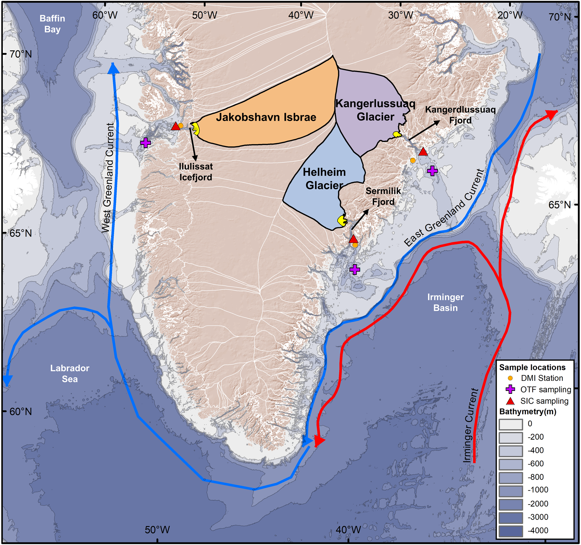
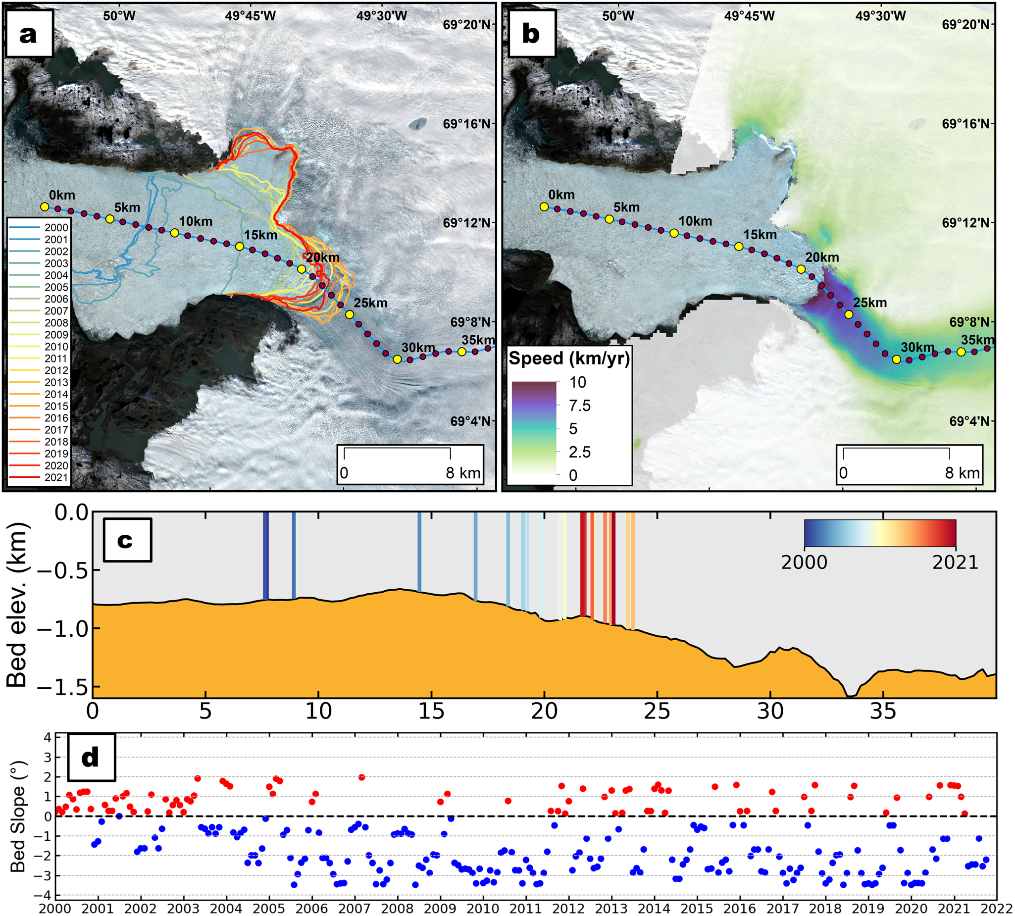
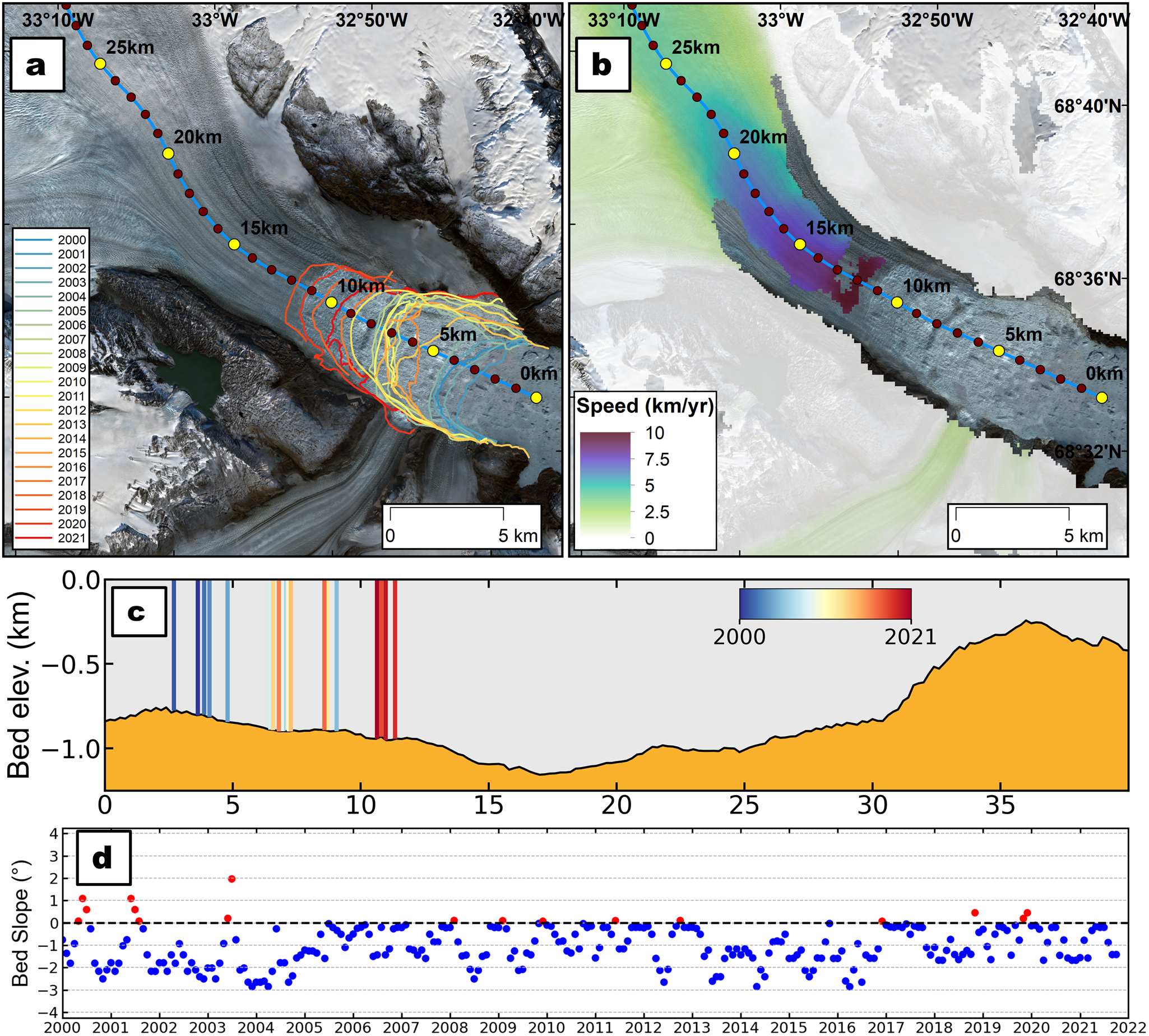
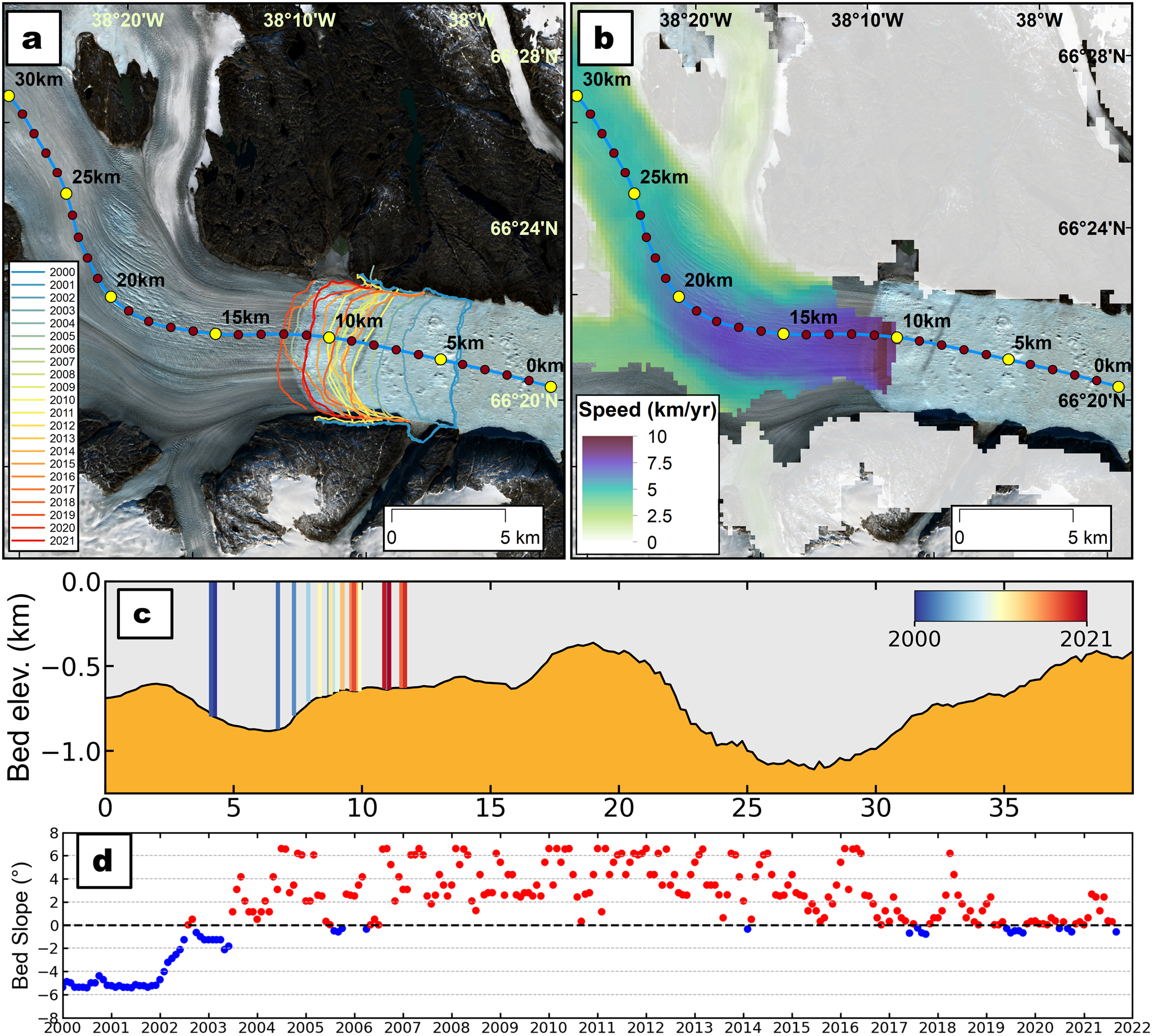
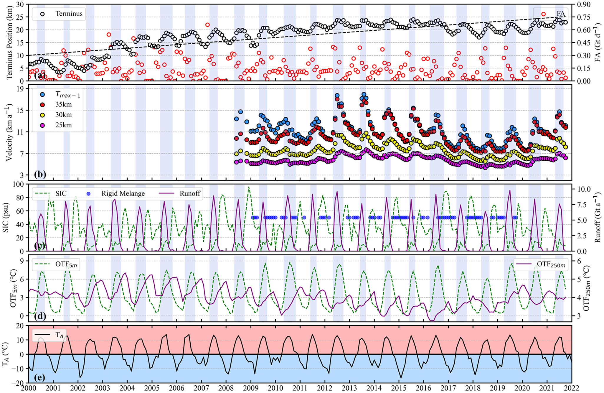
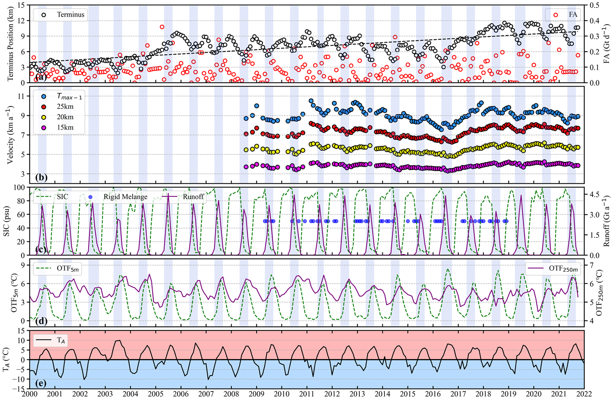
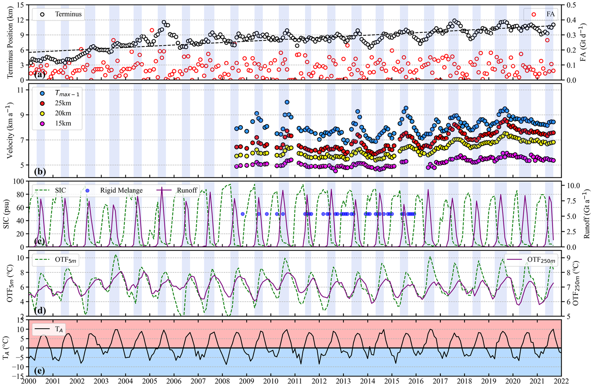
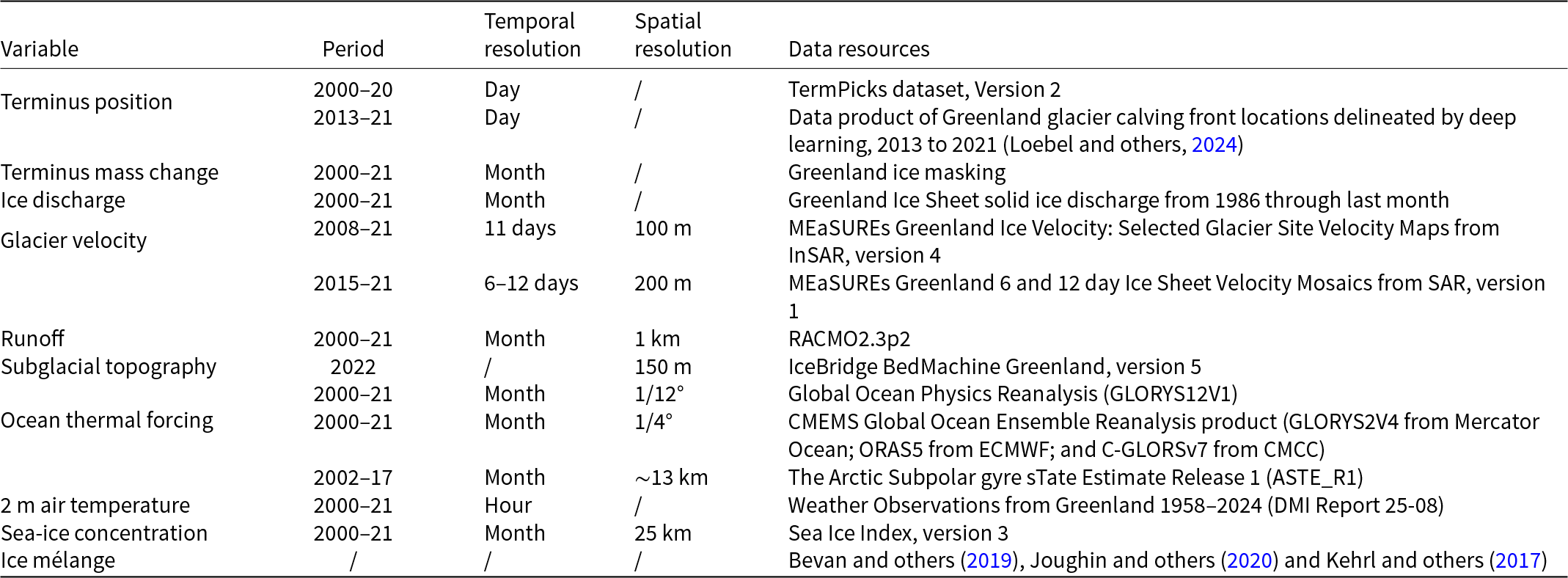
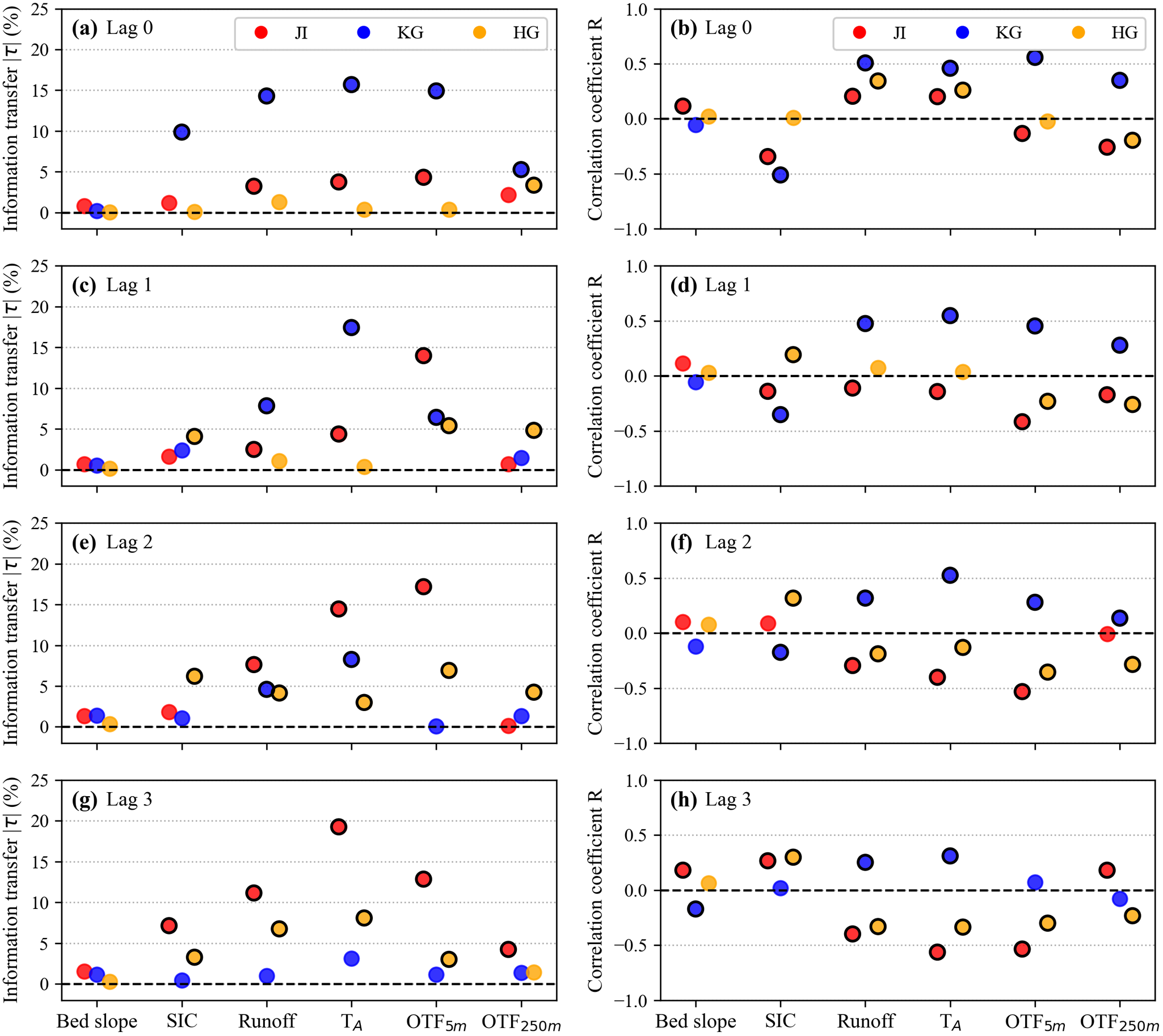
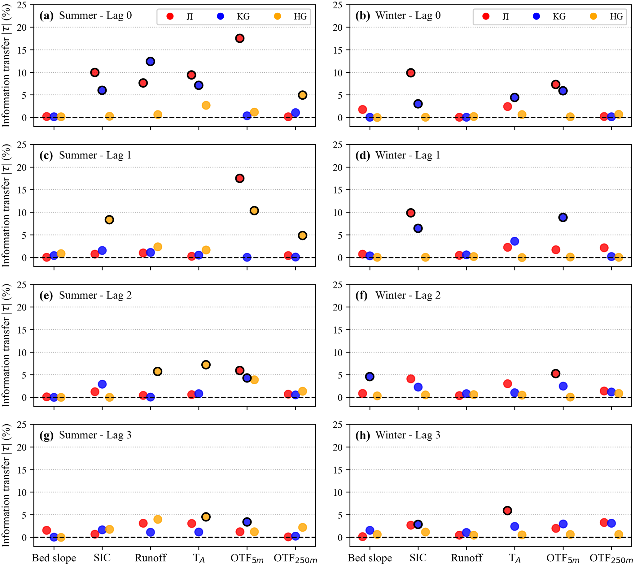
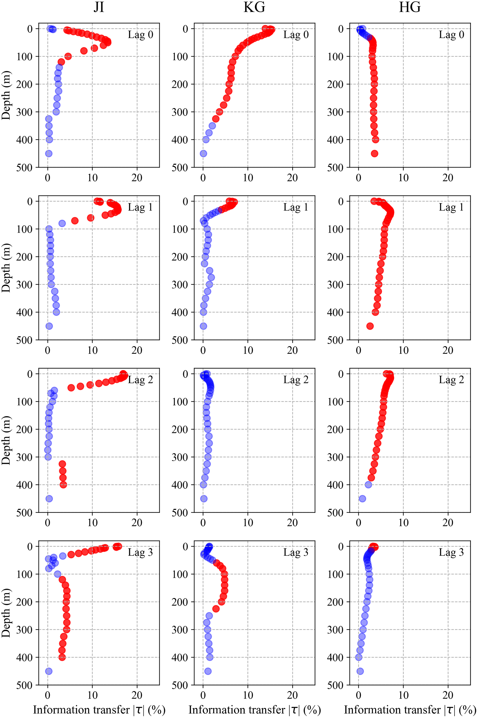

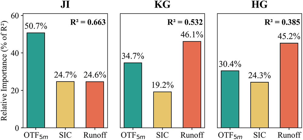
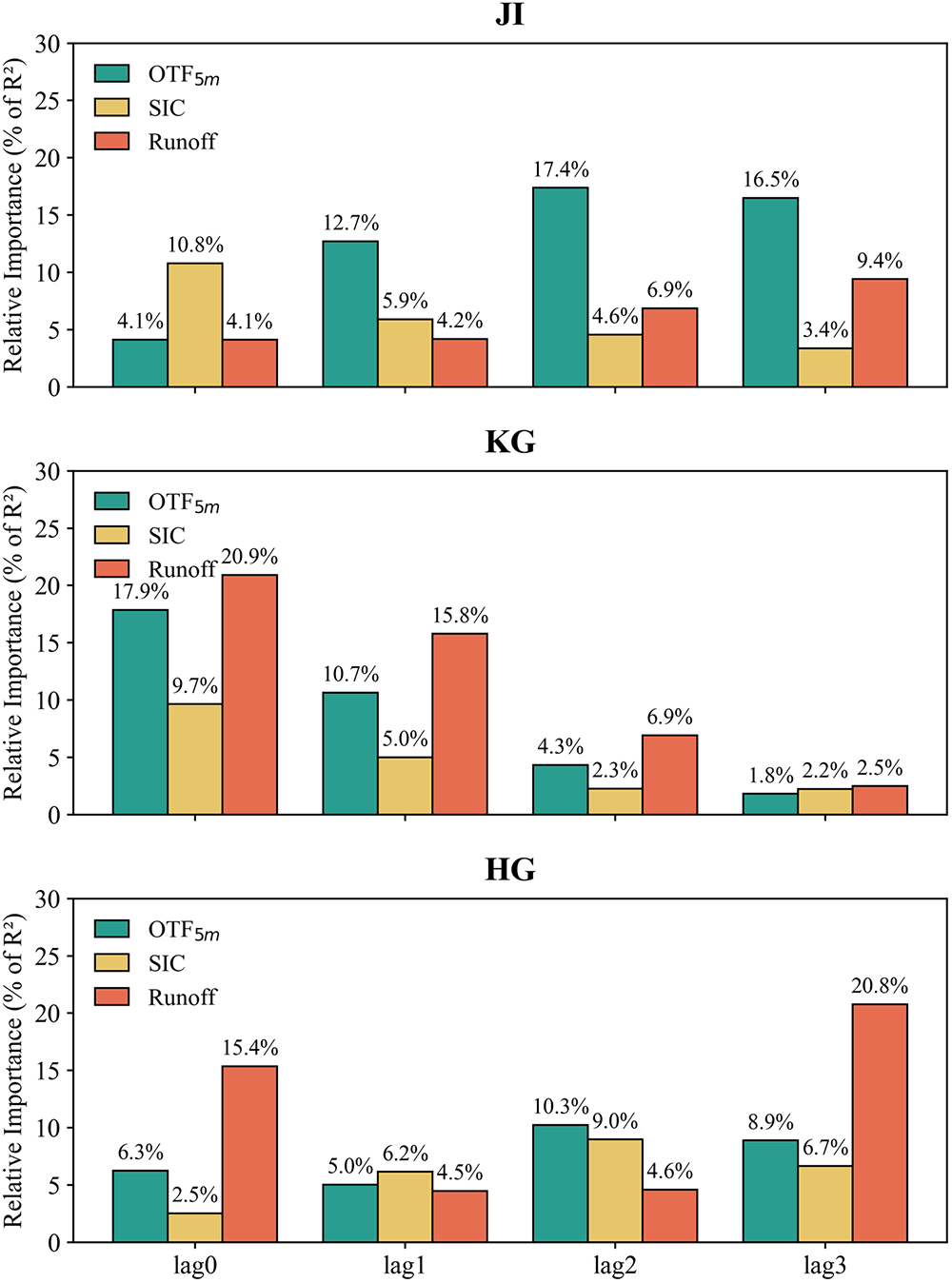


 Open access

