


1. Introduction
Glaciers and ice sheets are important components of the environment at high altitudes and latitudes due to their interactions with the atmosphere, ocean and periglacial environments. To explain the past and present changes in the glaciated regions and predict their evolution in a changing climate it is necessary to understand the processes of mass and energy exchange at and below the surface of glaciers (e.g. Haeberli and others, Reference Haeberli, Hoelzle, Paul and Zemp2007). Several of such processes occur when liquid water at the glacier surface interacts with the often subfreezing snow and firn.
Infiltrating liquid water at glaciers is often refrozen and retained in snow and firn. The processes significantly reduce the fraction of meltwater that contributes to runoff from large areas of both ice sheets and glaciers (e.g. Noël and others, Reference Noël2017, Reference Noël2018; van Wessem and others, Reference van Wessem2018). Rates of water refreezing and retention are controlled by the availability of liquid water as well as by the spatial distribution of subsurface temperature, density and water content. These parameters can, in turn, be significantly altered by infiltrating water. Quantification of the mass and energy fluxes involved in the interaction between water and porous snow/firn layers is further often complicated by preferential water flow. According to field observations (e.g. Williams and others, Reference Williams, Erickson and Petrzelka2010) water flows not only vertically, but also horizontally, and the rate of flow can be highly spatially variable.
Refreezing can occur both during the melt season, when the water enters the subfreezing environment and after it, when the water retained by capillary forces against gravity is refrozen as the winter cold wave penetrates downwards (e.g. Golubev, Reference Golubev1975). In all cases refreezing is associated with the release of latent heat and thus subsurface temperature can be used as a measurable proxy (e.g. Pfeffer and Humphrey, Reference Pfeffer and Humphrey1996; Humphrey and others, Reference Humphrey, Harper and Pfeffer2012). The current study focuses on estimating the potential of firn to retain water in pores as its refreezing is an important component of the climatic mass balance (e.g. Schneider and Jansson, Reference Schneider and Jansson2004; Reijmer and Hock, Reference Reijmer and Hock2008; Van Pelt and others, Reference Van Pelt2019). Results from a simulation covering glaciers of the Kongsfjorden area in Svalbard further illustrate the point: average refreezing rate during melt seasons of 1961–2012 was 0.13 m w.e. a−1 while for the cold periods the corresponding value is 0.16 m w.e. a−1 (Van Pelt and Kohler, Reference Van Pelt and Kohler2015). The amount of liquid water in snow/firn can be expressed as either a gravimetric (Θm = m w/m s) or volumetric (Θ = V w/V s) fraction of a sample, where m s and V s are the mass and volume of a sample and m w and V w are the mass and volume of liquid water therein (Jordan and others, Reference Jordan, Albert, Brun, Armstrong and Brun2008; DeWalle and Rango, Reference DeWalle and Rango2008). The two terms are related as: Θ = Θm · ρ/ρ w, where ρ w and ρ are densities of the sample and of pure water. An alternative way to describe the amount of water in snow/firn is through the water saturation of pores (S) which is the relation between the volumes of water and pores in a sample. It is related to the water content as: S = Θ/p = Θ/(1 − (ρ − Θm · ρ)/ρ i), where p is porosity and ρ i is the density of ice (Schneider and Jansson, Reference Schneider and Jansson2004). Other commonly used terms are the irreducible liquid water content and saturation (Θir and S ir) describing the amount of water remaining in the snow/firn when all free water is drained (Coléou and Lesaffre, Reference Coléou and Lesaffre1998; DeWalle and Rango, Reference DeWalle and Rango2008). These parameters are usually included in multilayer snow and firn models coupled to the surface mass and energy flux formulations and possibly incorporated in regional climate models (e.g. Steger and others, Reference Steger2017). A common assumption is that liquid water enters each next layer only after the current layer is at 0°C and water storage equals the irreducible liquid water content (e.g. Van Pelt and others, Reference Van Pelt2012). Liquid water content of snow and firn is challenging to measure due to the subtle thermodynamic balance inherent to mixes of two different phases of the same material (e.g. Colbeck, Reference Colbeck1978; Boyne and Fisk, Reference Boyne and Fisk1987). Several techniques utilizing different physical principles have been applied for the task. A group of methods is based on the effects occurring when the liquid water contained in the pores of a sample is subjected to either thermal or chemical forcing. In the first case, the thermal and phase change feedback of a sample subjected to a precisely dosed external cooling (Jones and others, Reference Jones, Rango and Howell1983; Coléou and Lesaffre, Reference Coléou and Lesaffre1998) or heating (Kawashima and others, Reference Kawashima, Endo and Takeuchi1998) is measured. In the latter case, the pore water in firn is diluted by a solution of dye (Grenfell, Reference Grenfell1986) or salt (Davis and others, Reference Davis, Dozier, LaChapelle and Perla1985; Schneider and Jansson, Reference Schneider and Jansson2004) and the change in concentration is measured. Alcohol calorimetry suggested by Fisk (Reference Fisk1986) is essentially a combination of the two approaches. Wet snow consists of ice, liquid water and air, which all have different dielectric permittivity allowing to solve for the liquid water content using a mixing model (e.g. Looyenga, Reference Looyenga1965; Denoth and others, Reference Denoth1984; Tiuri and others, Reference Tiuri, Sihvola, Nyfors and Hallikaiken1984; Roth and others, Reference Roth, Schulin, Flühler and Attinger1990) and measured density and permittivity of the snow/firn pack. The latter can be measured using capacitive sensors (e.g. Denoth, Reference Denoth1994), parallel-wire transmission-line resonators (e.g. Sihvola and Tiuri, Reference Sihvola and Tiuri1986), ground-penetrating radars (Mitterer and others, Reference Mitterer, Heilig, Schweizer and Eisen2011a; Heilig and others, Reference Heilig2015), time-domain reflectometry (Schneebeli and others, Reference Schneebeli, Coléou, Touvier and Lesaffre1998; Samimi and Marshall, Reference Samimi and Marshall2017) or GPS receivers placed above and below the snowpack (Koch and others, Reference Koch, Prasch, Schmid and Schweizer2014; Schmid and others, Reference Schmid2015). Recently Adachi and others (Reference Adachi, Yamaguchi, Ozeki and Kose2020) used magnetic resonance imaging to derive the water content of snow in three dimensions and with a high spatial resolution. The reported estimates of the snow and firn liquid water content vary from 0 to ~15 vol.% (e.g. DeWalle and Rango, Reference DeWalle and Rango2008) with a general tendency to increase in response to the supply of liquid water (e.g. Mitterer and others, Reference Mitterer, Hirashima and Schweizer2011b). The amount of irreducible water in snow/firn is known to reduce with density (Coléou and Lesaffre, Reference Coléou and Lesaffre1998). According to Schneider and Jansson (Reference Schneider and Jansson2004) for ρ values of 400 and 700 kg m−3 Θ ir is 4.24 and 2.33 vol.%. The parameter is often reported as saturation fraction S ir and values range from 0.07 (Colbeck and Anderson, Reference Colbeck and Anderson1982) to 0.04 (Jordan and others, Reference Jordan, Andreas and Makshtas1999) and even 0.01 (Jordan and others, Reference Jordan, Albert, Brun, Armstrong and Brun2008). For the above ρ values (400 and 700 kg m−3) S ir = 0.07 corresponds to Θir of 4.05 and 1.7 vol.%, while S ir = 0.04 to 2.28–0.95 vol.% respectively. At the same time in a widely applied SNOWPACK model (Bartelt and Lehning, Reference Bartelt and Lehning2002) Θir was initially a constant equal to 8 vol.%. Motivated by the scarcity of the water content estimates from firn, two new methods for deriving the parameter are presented. Both methods are based on quantification of the latent heat released by the water refreezing in pores as the freezing front propagates downwards during autumn. The methods are applied using the subsurface temperature and density measured at Lomonosovfonna, Svalbard, during April 2014–16 (e.g. Marchenko and others, Reference Marchenko2017b). We present the reconstructed liquid water fractions and discuss possible implications for simulating the subsurface processes by multilayer models.
2. Estimation of firn water content
Processes at the migrating transition from cold to temperate parts of the subsurface temperature profile including refreezing of pore water were earlier considered for solid ice at Jakobshavn Isbræ (Lüthi and others, Reference Lüthi, Funk, Iken, Gogineni and Truffer2002) and at Storglaciären (Pettersson and others, Reference Pettersson, Jansson and Blatter2004). There, the migration of the freezing front is driven by the vertical advection of ice upwards occurring in the ablation areas of glaciers and ice sheets. In this study we address freezing of pore water driven by the upward-directed subsurface heat flux induced by the low surface temperature during the autumn and winter seasons. That process is also characteristic for the permafrost active layer. Nicolsky and others (Reference Nicolsky, Romanovsky and Tipenko2007) quantified the thermal conductivity, heat capacity and unfrozen water content of soil by iteratively optimizing the combination of parameters minimizing the misfit between the measured and simulated temperature.
Here, we focus on the propagation of the winter cold wave and freezing front (or cold-temperate transition – CTT) downwards. By that time surface melt largely ceases and the amount of water stored in firn pores cannot be expected to increase. Quantification of the firn water content is based on the analysis of the rate of CTT propagation under different assumptions and thus CTT is a key parameter for the study. Here, it is defined as the depth above which the entire profile is colder than the temperature of water freezing T 0, is assumed to be equal to − 0.03°C. Temperature measurements are subject to uncertainties and using a higher value results in an unrealistically uneven and discontinuous pattern of CTT propagation, which complicates quantitative analysis (see the green curve in Fig. 1b). Here, we assume that a change in the CTT depth is governed by two processes: the vertical conductive heat flux and refreezing of liquid water in the pores of firn through which the freezing front advances. Thus, low effective thermal conductivity and large water content result in a reduced rate of freezing front propagation. The process is similar to the zero curtain effect in seasonally freezing soils and permafrost (Outcalt and others, Reference Outcalt, Nelson and Hinkel1990). Two different implementations of the approach are employed for quantification of the firn water content: optimization and ‘direct’ calculation. Both of them rely on the same empirical dataset and forward model described below. Within the optimization method we attempt to minimize the misfit between the measured and simulated depths of the freezing front by adjusting the mass of water assumed to be present in the subsurface profile at the start of the cold season. The ‘direct’ quantification of water mass in firn is based on conversion of the difference in firn temperature between measurements and simulation assuming zero water content.
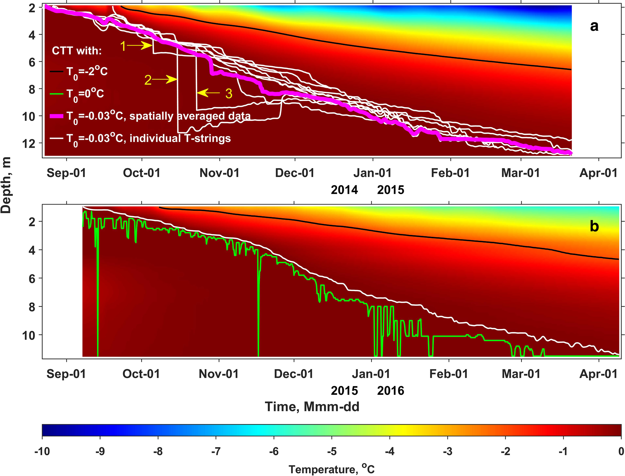
Evolution of subsurface temperature measured at Lomonosovfonna in fall–winter 2014/15 (a) and 2015/16 (b). Note: panel a shows horizontally-averaged data from nine T-strings and panel b data from a single T-string. Also shown are the − 2°C isotherm (black curves), the propagation patterns of the CTT based on ice melt temperature T 0 = −0.03°C derived from the horizontally-averaged temperature data (thick magenta curve) and from the individual T-strings (thin white curves). The green curve in panel b shows the CTT based on ice melt temperature T 0 = 0°C. Yellow numbered arrows point to rises in CTT depth, details are given in Fig. 5.
2.1. Empirical data and post-processing
The results presented below are based on the empirical data collected at Lomonosovfonna, Svalbard (78.824° N, 17.432° E, 1200 m a.s.l.). This includes measurements of firn temperature, firn density and air temperature. We use data from nine thermistor strings (T-strings) installed in April 2014 in a 3×3 square pattern with a lateral spacing of 3 m and from a single T-string installed in April 2015. The same raw data were earlier presented by Marchenko and others (Reference Marchenko, Pohjola and Pettersson2019b) and used to constrain a parameterization of preferential water flow in firn and an optimization of effective thermal conductivity of firn (Marchenko and others, Reference Marchenko2017b, Reference Marchenko2019a). The data are available at https://github.com/SergeyMarchenko/FirnWaterCodesGit along with two Matlab apps for interactive visualization (see Supplementary material for details). Here, we use the temperature measurements covering the autumn and winter seasons of 2014/15 and 2015/16 and done in the depth range from 0.5 to 12 m referenced to the glacier surface at the time of T-string installation (Fig. 1). The T-strings installed earlier had 11–15 sensors spaced by 0.5–2 m, the later T-string had 31 sensors spaced by 0.25–1 m (see the Fig. S1 in Supplementary material for further details).
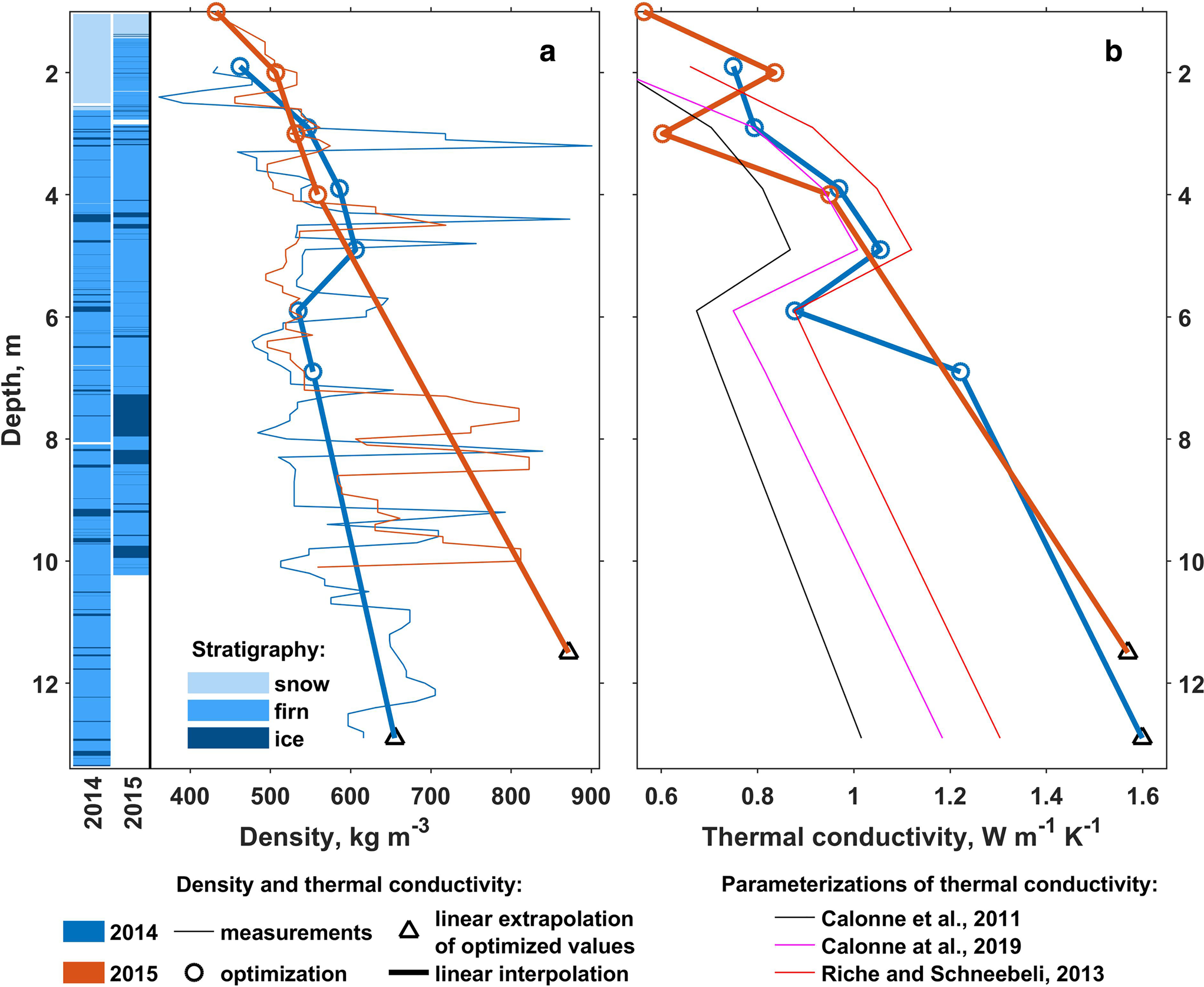
Post processing of the firn temperature data included several steps. First, readings from most individual sensors were calibrated against 0°C by introducing offsets defined as the mode of values during the time period, when the temperature is expected to be at 0°C. The periods are defined for individual sensors based on subjective data analysis: in most cases readings from individual thermistors plotted as a function of time show a distinctive upper threshold and have kinks just before and after it. The mean and mean absolute offsets are respectively − 0.01 and 0.06°C. In a second step temperature values were linearly interpolated to an even time grid spaced by Δτ~ = ~6 h. This was followed by low-pass filtering with 12 h cut-off threshold to eliminate the high-frequency fluctuations. Finally, the values were interpolated to a 0.1 m-spaced vertical grid using piecewise cubic interpolation. The values measured in 2014/15 were laterally averaged to produce one more data series, which is expected to be more laterally representative than data from individual T-strings. Positive temperature values in all data were deemed unrealistic and were reset to 0°C (see Supplementary material for further discussion on the calibration of temperature data and positive T values). Along with that we employ air temperature measurements done at the site using a Rotronic HC2S3 sensor during April 2014–2015 and data from shallow firn cores drilled in April 2014 and 2015 (Fig. 2a). The firn density data along with description of the routines applied in the field and cold chamber were presented by Marchenko and others (Reference Marchenko2019c). The water content calculations described below rely on effective thermal conductivity k eff and density ρ of firn (Fig. 2) derived using optimization techniques following Marchenko and others (Reference Marchenko2019a). For that we use measured subsurface density (thin blue and red curves in Fig. 2a and temperature values (Fig. 1) colder than − 2 °C, since we would like to minimize the influence of refreezing processes on the inversion routine. The optimization starting in fall 2014 is based on horizontally-averaged T data and for the 2015 season we use the measurements from the single available T-string. The optimized k eff and ρ values (red and blue circles) are spaced by 1 m and are vertically limited by the maximum depth of the − 2°C isotherm. Therefore, k eff and ρ at the bottom of the calculation domains (black triangles in Fig. 2) were determined by linear extrapolation of the optimized values and linear interpolation was applied to constrain the parameters at the nodes of the regular 0.1 m-spaced grid applied in water content calculations (thick red and blue curves in Fig. 2). We use the glacier surface in April 2015 as a common zero reference for the vertical axis. The vertical offset between glacier surfaces in April 2014 and 2015, when the T-strings were installed, is estimated to be 0.9 m. The value minimizes the misfit between temperature profiles simultaneously measured in April 2015 using the earlier and later T-string installations and vertically referenced to the glacier surface at the day of deployment.
Subsurface density (ρ) and stratigraphy (a) and thermal conductivity (k eff, b) at Lomonosovfonna. The parameterized k eff values are calculated following Calonne and others (Reference Calonne2011), Calonne and others (Reference Calonne2019) and Riche and Schneebeli (Reference Riche and Schneebeli2013). The optimized k eff and ρ values are calculated following Marchenko and others (Reference Marchenko2019a).
2.2. Forward model
The forward model used in both methods of firn water content quantification describes the processes of conductive heat flow and water refreezing in firn. The model is 1-D and at every time step it first calculates firn temperature changes due to heat conduction and then assesses the effect of water refreezing on the subsurface temperature and water content. Thermal conduction is approximated using Fourier's law:

where the medium properties C, ρ, T and k eff are the specific heat capacity (J (kg °C)−1), density (kg m−3), temperature (°C) and effective thermal conductivity (W (m °C)−1), respectively. Variables τ and z are the time (s) and vertical space (m) coordinates. A temperature-dependent function is used to approximate the values of specific heat capacity (Cuffey and Paterson, Reference Cuffey and Paterson2010). The conduction Eqn (1) is numerically solved using an explicit forward in time and central in space finite difference scheme. Refreezing of pore water occurs in a layer i if it is both cold (T i < T 0) and wet (m i > 0) Here, m i is the mass of water in pores in kg m−2. As a result of that both the temperature and water mass within the layer change according to:

and

where $T_{ i}^r$ and $m_{ i}^r$
 are the updated temperature and pore water mass of the layer. It can be noted that it is assumed that density of firn layers does not change in time. The initial temperature is constrained by the empirical data and the choice of initial water content is described below. The model is driven by the measured temperature fluctuations at the upper boundary of the domain. The lower boundary conditions is constrained by measured temperature values. The subsurface snow/firn profile is represented by multiple layers with thickness Δz = 0.1 m. The extent of simulation domain in the vertical direction and in time depends on the pattern of measured CTT propagation and thus varies between T-strings and years. In all cases the uppermost point of the grid lies at the depth of 1 m referenced to the glacier surface at the time of T-string installation and typically the domain extends down to 12 m and covers the time period from September to April. To ensure numerical stability of the finite difference scheme used for solving the conduction equation the Courant–Friedrichs–Lewy (CFL) condition (Dahlquist and Björck, Reference Dahlquist and Björck2012) is checked on every time step. If k eff,i~Δτ/ρ i~C i~Δz 2 > 0.45 for any of the layers, then auxiliary iterations of the entire forwards model are done on a finer time grid. The additional calculations are constrained by linearly interpolated upper and lower boundary conditions of the domain. In case the CFL condition is not fulfilled with the standard time step, it is essential to include both the conduction and refreezing parts of the forward model into the loop of additional iterations. This will force consecutive refreezing of water in layers and ensure that no phase transitions occur in the layer between z i and z i+1 before all water above z i is refrozen and the measured CTT reaches it.
2.3. Method 1: optimization of water content
The optimization routine uses the above described model as the forward model. Executed in multiple steps, it consecutively optimizes the elements of the vector m i, i = 1…nl defining the water mass contained in the pores of firn layers (nl is the number of layers) at the start of the simulation. At an optimization step i the mass of water $m_{ i}^{opt}$ in a layer i bound by depths z i and z i+1 is found as the argument minimizing the absolute value of the cost function Q i:

where

Here, z CTT,s (m, τ) and z CTT(τ) are respectively the simulated and measured depths of the freezing front. The first one is controlled by the assumed initial water content profile and both depend on time. The comparison is done only at the time steps when the measured CTT penetrates through the layer i: from $\tau ^{CTT}_{z_{ i}}$ to $\tau ^{CTT}_{z_{i + 1}} - \Delta \tau$
 when the CTT is found just below and just above the depths z i and z i+1, respectively. With an increase of the assumed water mass m i the cost function Q i decreases but only to a certain threshold after which additional water has no effect on the rate of CTT propagation. Equation (4) is solved using the bisection algorithm (Dahlquist and Björck, Reference Dahlquist and Björck2008) with 0 and 10 kg m−2 as the lower and upper margins of the initial search window. At the first optimization step quantifying the water mass in the topmost layer the initial water content in all layers is 0 kg m−2. Starting from the second optimization step the initial water content profile includes the water masses $m^{opt}_1$
 …$m^{opt}_{i-1}$
 from all previous optimization steps, while all other layers (m i …m nl values) are initially assumed to have no water. It can also be noted that implementation of the forward model on a vertical grid with layers having finite thickness results in a step-wise propagation of the CTT: it is always found at the boundaries between layers. This complicates the use of some optimization techniques as the derivative of the cost function dQ i/dm i (Eqn (4)) is discontinuous. In ≈ 9% of all cases the cost function Q i is negative even for m i = 0 kg m−2 suggesting that at the corresponding time steps the simulated rate of CTT propagation is lower than the measured one even if there is no water holding it back. These situations are associated with exceptionally high rates of measured CTT propagation, occasional drops in the CTT can be seen in Fig. 1 and some of them are discussed in the Discussion section and in the Supplementary material. In that case $m^{opt}_{ i}$
 is set to 0 kg m−2. A side effect of using 0 as the initial guess for the water mass in layers below the one for which the optimization is done at step i (m i+1 …m nl) is that the optimization routine tends to overestimate $m^{opt}_{ i}$
 to prevent the freezing front from penetrating too deep as below there is no water that could impede the CTT propagation. Therefore, the whole optimization routine is repeated several times and at each next repetition results from the previous one are used as the initial condition for the water content profile. Typically, the m opt values settle down after four iterations. This is illustrated in Fig. 3: the sum of differences between the water mass profiles returned by two consecutive optimization iterations n and n − 1 ($\sum m^{opt}_n - m^{opt}_{n-1}$
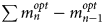 ) decreases with increasing n and changes only slightly after n reaches five. The overall negative range of values suggests that the vertically integrated mass of water decreases with every optimization iteration. To speed up the calculation of water content for all optimization steps starting from i = 3 the number of time steps for which the forward model is run was reduced. First, the simulation starts from $\tau ^{CTT}_{z_{i-1}} - \Delta \tau$
 , which is when the data-derived CTT is found just above the depth z i−1. Second, the simulation stops at the time step $\tau ^{CTT}_{z_{i + 1}} - \Delta \tau$
 when the measured freezing front is just above z i+1. In that case the initial temperature and water content profiles are constrained by values derived at the end of the forward model run using $m^{opt}_1 \ldots m^{opt}_{i-1}$
 values from the previous optimization steps.
Influence of multiple optimization iterations on the optimized water masses. The vertical axis shows the sum of differences in water mass profiles derived in consecutive iterations of the optimization routine. The thick black curve corresponds to the horizontally-averaged data from 2014, thin curves are from the individual T-strings installed in April 2014 and 2015.

2.4. Method 2: ‘direct’ calculation of water content
For the ‘direct’ estimates of firn water content (see Fig. 4a) we use measured temperature T k (black curve) at time step τk to predict the temperature profile at the next time step (τk+1) assuming that thermal conduction is the only mechanism of heat transfer. For that we use the above described forward model (Eqn (1)) and set the water content m to zero. The misfit:

between the simulated ($T^{s}_{k + 1}$ ) and measured (T k+1) temperature profiles at time τk+1 (dashed green and solid blue curves respectively) is related to the effect of meltwater refreezing as the observed CTT advances from depth $z^{CTT}_k$
 (black triangular marker) to depth $z^{CTT}_{k + 1}$
 (blue triangular marker). The dT k+1 values (Fig. 4b) exhibit positive values along the measured CTT (shown by the black curve), which is interpreted as an effect of refreezing not captured by the model. For every time step the anomaly is defined as a series of positive values that monotonically decrease away from a maxima found within 0.5 m from the measured CTT. In Fig. 4b the vertical limits of the dT anomaly for each time step are indicated by the blue (upper, z t), red (lower, z b) and green (in case z t = z b) markers. If the simulated freezing front $z^{CTT, s}_{k + 1}$
 is deeper than the measured one $z^{CTT}_{k + 1}$
 (green and blue triangular markers in Fig. 4a), then the positive dT k+1 values bound by the depths z b and z t are converted to the corresponding water masses as:

After that m k, k = 2…nτ values are summed in groups in accordance with the depths of the measured CTT depth at time moments τ2…τnτ, where nτ is the number of time steps in the domain, to produce the profile of water masses in 0.1 m-thick depth intervals.
‘Direct’ calculation of the mass of liquid water in firn. (a) Conceptual model illustrating typical measured (T) and simulated (T s) temperature profiles at time steps τk and τk+1 and corresponding CTT depths. For the purposes of illustration the simulation time (τk+1 − τk) was $\gg$ 6 h. (b) Difference between simulated and measured temperature profiles (dT k+1, see Eqn (6)) for one of the individual T-strings installed in 2014.

3. Results
The evolution of subsurface temperature measured at Lomonosovfonna is presented in Fig. 1 for fall–winter 2014/15 (a) and 2015/16 (b). At the start of simulations (late August–early September) temperate firn is found along the entire depth of the firn profile. At the same time according to three T-strings on the 1st of September 2014 firn at subfreezing temperature was present below the depth of 5 m. The same conditions were measured in 2015. These cold pockets largely disappeared by mid-October due to heating from adjacent warmer firn volumes. Due to cooling at the surface the firn temperature gradually decreases and reaches negative values all the way down to 10–12 m by April of the next year. The only notable deviation from the dominating cooling tendency is observed around the 18th of September 2014, when temperature rose above − 1°C down to the depth of ~1.7 m. The phenomenon can be interpreted as a response to a preceding surface melt event, as on the 16th of September the measured air temperature was above − 0.3°C during 12 h, while the mean value during 10–20 September was − 7.8°C. The measured patterns of CTT propagation are shown in Fig. 1. The average rate of daily CTT subsidence for all temperature datasets is 5.5 cm d−1 with a prominent variability across time and different T-strings: from − 1.04 to 6.75 m d−1. While the standard deviation in daily CTT propagation rates averaged for individual T-strings installed in 2014 is not large, 0.52 cm d−1, from Fig. 1a it is apparent that freeze-up of the firn is not homogeneous in space. That is confirmed by the mean standard deviation of simultaneous CTT depths for different T-strings (0.71 m). Assuming a constant temperature gradient above the freezing front, lower rates of CTT propagation can be interpreted as being caused either by an increase of the firn water content or by a decrease of the effective thermal conductivity in the corresponding depth interval. For example, around the 12th of November 2015 there is a notable kink in the CTT curve from the horizontally-averaged data (magenta curve in Fig. 1b). Before that date, the daily CTT propagation rate is ~3.7 cm d−1, while after it is 5.4 cm d−1. The step-wise behaviour of the curves based on data from single T-strings is even more pronounced as the temperature signal recorded by individual arrays of sensors comes from a smaller volume of firn and is thus more affected by the spatial heterogeneity in its properties.
The prominent jumps of 0.5–5 m seen in the depths of CTT derived from individual T-strings (e.g. on the 5th of October 2014) are marked by numbered arrows in Fig. 1a. The relevant temperature data is presented in detail in Fig. 5. As it appears from the figures, the magnitude and the pattern of temporal change in readings from sensors at some depths (4.75 m in T-string 1, 5.65–7.65 m in T-string 4 and 5.85–8.85 m in T-string 5) suggest that firn adjacent to them did not experience the direct influence of liquid water and remained dry. At the same time thermistors placed above and below the named depth intervals show signs of water presence: measured temperature remains at one level during at least 1 week, which is followed and in most cases preceded by steep cooling and warming respectively.
Temperature measured by individual sensors at T-strings n. 1 (a), 4 (b) and 5 (c) installed in April 2014 and explaining the abrupt increases in the CTT depth labelled ‘1’, ‘2’ and ‘3’ in Fig. 1a. Note: the data shown here is not low-pass filtered.
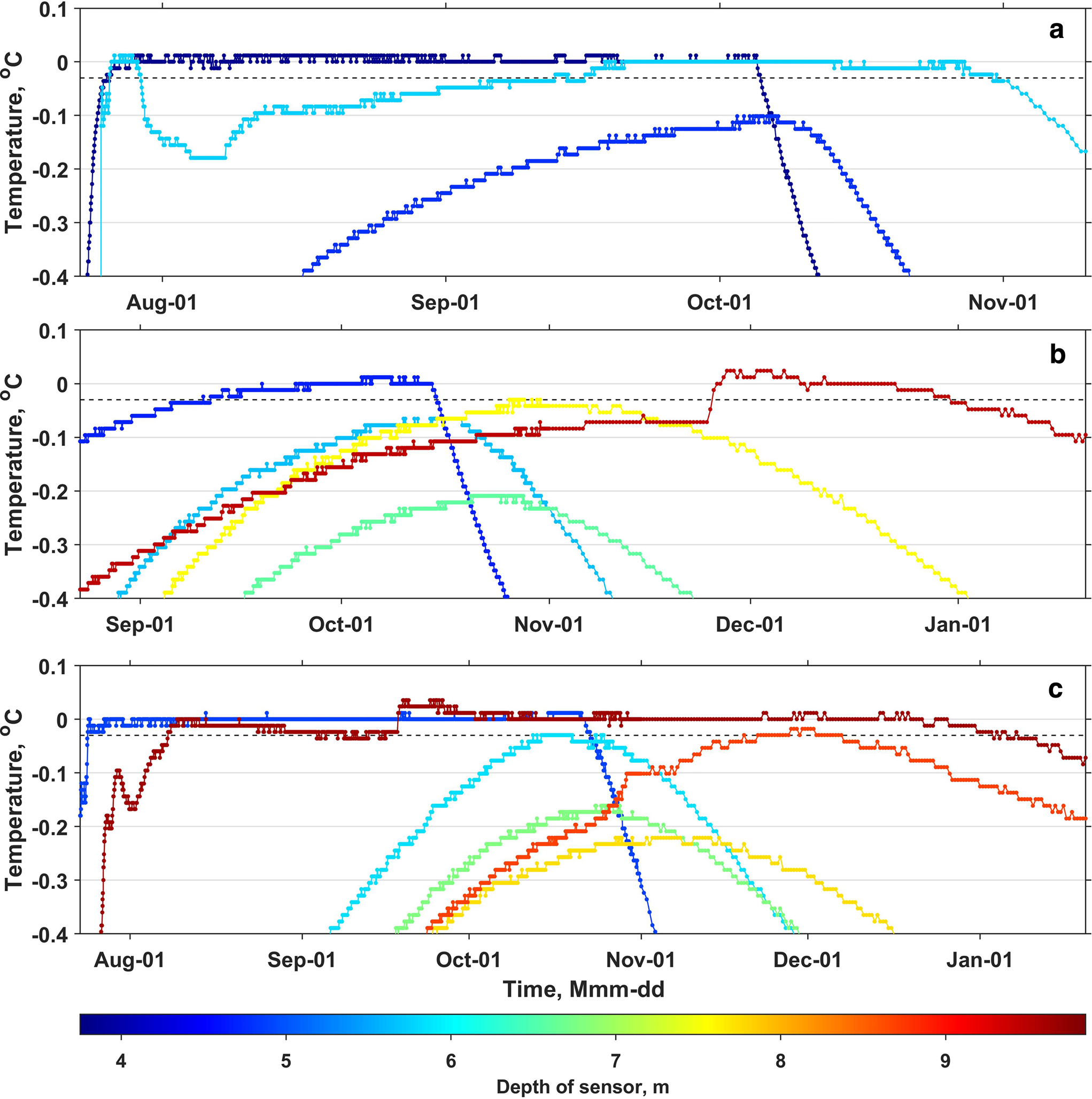
Figure 6 shows relative volumetric water content (Θ in vol.%) calculated using different datasets (b) and methods (a, c). The general pattern in the vertical variability of water content is that the values are higher in the upper part of the profile and significantly lower deeper down. In most cases the optimized Θ values are well below 1 vol.%. The local maxima in water content profiles derived from single T-string data (blue and red curves in panel b) reach up to 3 vol.%. Prominent spikes (> 0.5 vol.%) can be seen all the way down to the depth of 8 m. These last phenomena are observed mainly in results based on data from individual T-strings: water content from the laterally-averaged dataset (black curve) expectedly exhibits lower peak values while fewer firn layers have no water, especially higher up in the profile. Compared to the Θ values for 2014/15 (blue curves in Fig. 6b, the volumetric content calculated for the fall–winter 2015/16 season (red curve) is considerably lower: the peaks in the upper part of the profile are not that high and are absent below the 4 m depth. Although, it has to be said that half of the water content profiles from the earlier single T-strings does not have spikes above 0.5 vol.% below 5 m depth. As evidenced by Fig. 6a in most cases Θopt and Θdir profiles exhibit similar vertical dynamics with spikes appearing at the same depth intervals. However, the magnitude of maxima varies between results from the two methods. Figure 6c presents the relation between all the firn water content values calculated using both presented methods with Θopt and Θdir shown along the horizontal and vertical axis respectively. Note that here Θ values are averaged to a 0.2 m-spaced depth grid to exclude the influence of high-frequency fluctuations on the analysis. The high coefficient of determination (R 2 = 0.75) between Θopt and Θdir and low mean difference ($MD = {\mathbb E} ( \Theta ^{dir} - \Theta ^{opt}) = -0.01$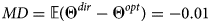 vol.%) suggest a decent match and low bias between values derived using these different methods. At the same time, for the layers where either Θopt ≥ 0.5 vol.% or Θdir ≥ 0.5 vol.% (red dots in Fig. 6c) the linear dependence between data series is not that strong (R 2 = 0.47), while MD remains low 0.01 vol.%). The total water mass calculated for nine domains based on data from individual T-strings installed in 2014 is on average 14.9 kg m−2 for optimization and 14.5 kg m−2 for the ‘direct’ method, while the respective standard deviations are 3.4 and 2.4 kg m−2.
Volumetric water content of firn at Lomonosovfonna quantified using different temperature datasets and methods. (a) Results derived using laterally-averaged firn temperature from fall 2014. Optimized values (Θopt) – black curve, results from the ‘direct’ method (Θdir) – light-blue curve. (b) Optimized values (Θopt) for the single T-string data from fall 2014 (blue curves) and fall 2015 (red curve). Also shown are Θir values calculated following Schneider and Jansson (Reference Schneider and Jansson2004) as a function of density (green). (c) Dependence between optimized (Θopt) and ‘directly’ calculated (Θdir) volumetric water content values. Results are averaged for 0.2 m depth intervals. Red markers highlight the points where Θopt or Θdir are ≥0.5 vol.%.

The thermal conduction Eqn (1) suggests that assumptions regarding both the thermal conductivity (k eff) and density (ρ) profiles have an impact on the water content estimates. Sensitivity of our results to perturbations in the parameters was separately tested by running both methods for the laterally-averaged data from fall 2014 using the thermal conductivity $k_{eff}^p$ parameterized following (Calonne and others, Reference Calonne2019) (magenta curve in Fig. 1b and density ρ p from shallow core measurements (blue curve in Fig. 1a) in place of optimized values (Fig. 7). The relative perturbations in thermal conductivity (dk eff) and density (dρ) are shown by the black curves in panels a and b respectively and the feedback of the water content values (dΘ) by the blue curves for optimization and red curves for the ‘direct’ method. The values are expressed in % and calculated as:

where the terms with superscript p are the perturbed values.
Relative sensitivity of the water content profiles quantified using the optimization (blue) and ‘direct’ (red) methods to perturbations (black) in the thermal conductivity (a) and density (b) used in the forward model (8). Note that the sensitivity of Θdir goes outside of the axis limits: up to 60% for k eff (a) and between − 100 and 170% for ρ (b).

Lower parameterized thermal conductivities (− 21% on average) expectedly result in lower simulated water content values (Fig. 7a). The relative change in the results of the ‘direct’ method (− 30% on average) is closer to the k eff perturbations in terms of magnitude than the respective feedback of the optimization method (− 49% on average), while the latter is less vertically variable. The last observation also applies to the feedback of water content quantification methods to density perturbations (Fig. 7b). Optimization returns a more vertically smooth response, which is also less pronounced than that of the ‘direct’ method and then the magnitude of the perturbation itself: the corresponding mean absolute values are 3, 13 and 11%.
4. Discussion
4.1. Methods for water content quantification
The methods presented above rely on measurements of subsurface temperature and density and on assumptions regarding the effective thermal conductivity of firn k eff. They allow us to derive the mass of water left in the firn pores by the time when the freezing front reaches the layer in question during the cold season following the ablation period. Our approach can be seen as a variation of the cold calorimetry method making use of natural temperature fluctuations and applied to a large volume of firn. The Θ estimates for fall 2014 presented above are based on readings from multiple temperature sensors, covering an area of 36 m2, which makes the volume of our ‘samples’ much larger than in all earlier published experiments. At the same time the spatial resolution of our measurement system does not allow to resolve the 3-D pattern of water refreezing. The latter likely occurs at the scale of centimetres or tens of centimetres, while our sensors are spaced by 0.25–2 m vertically and 3 m horizontally. As a consequence, the results presented in Figs 6 and 7 may not be representative at 0.1 m vertical resolution, particularly the vertical position and magnitude of thinner peaks in Θ. It can be recommended to use T-strings with more densely placed sensors; alternatively, fibre optic temperature sensors can be employed for temperature measurements to be used for firn water content quantification (Selker and others, Reference Selker2006).
Both suggested methods use the same 1-D forward model. Its validity is undermined by the fact that the measured horizontal temperature gradients are not equal to zero. This can be illustrated by the lateral variability in the simultaneous CTT depths from individual T-strings (thin white lines in Fig. 1a). Yet, most contemporary models simulating processes in snow and firn and used within spatially distributed domains (e.g. Van Pelt and others, Reference Van Pelt2019) are 1-D and ways to describe essentially 3-D processes within these models are to be found.
The optimization method minimizes the mismatch between simulated and measured CTT depths by iteratively adjusting the water content in corresponding layers. Within the ‘direct’ Θ estimates the water mass is calculated by comparing the empirical firn temperature data with the output of conduction only model at discrete time steps. However, the process of latent heat release at the CTT is a continuous process sustaining the high temperature gradient just above the freezing front. As a result of that, the suggested method can be expected to have a bias towards underestimation of the water stored in pores and small time steps are advisable. Another potentially weak point of the ‘direct’ method is the formalization of the choice of the dT values (Eqn (6)) to be converted to water masses. Typical rates of conductive heat flux suggest that anomalies found further than several meters from the CTT should be excluded, but defining the exact threshold is challenging. On the other hand ‘direct’ calculations are much faster than the optimization: ~4 s and 3.5 min per domain respectively and implementation of the method is more straightforward. Since both suggested methods are based on analysis of the dynamics of the freezing front, the choice of ice melt temperature T 0 used to define its depth is important. Although the chosen value of − 0.03°C returns a steady CTT propagation pattern without multiple sudden spikes occurring with T 0 = 0°C (white and green curves in Fig. 1b), the temperature gradient above the 0 °C isotherm causes a vertical offset of the water content estimates upwards. When the real CTT 0 based on T 0 = 0°C reaches a water-rich layer, the CTT −0.03 based on T 0 = −0.03°C will be found at a distance dz above that level. The offset can be expected to decrease when the CTT goes through a layer with higher water content. Provided that the heat flux above CTT is stable, the event will increase the temperature gradient and thus bring CTT −0.03 closer to CTT 0. The opposite is to happen when the freezing front goes through a layer with less pore water. The phenomenon is seen in Fig. 1b. The offset dz can be quantified from the measured temperature profiles: the depth difference between CTT 0 and CTT −0.03 averaged for all time moments and temperature data series is 1.3 m. However, if we consider only the dz values that are below 1.5 m, which excludes most of the unrealistic spikes in CTT 0 obvious from the green curve in Fig. 1b, then dz equals 0.6 m. Performance of the water content quantification methods can be assessed by comparing empirical CTT depths with the values simulated using the forward model constrained by different assumptions regarding Θ and also k eff in firn. Figure 8 shows the results for the domain constrained by the initial and boundary conditions from the horizontally-averaged firn temperature measured in fall–winter 2014/15. The black curve shows the CTT simulated using the optimized water content profile, the curve basically overlies the data-derived CTT (red) and can thus be taken as reference. The light-blue curve shows the CTT resulting from simulation using the water content profile derived using the ‘direct’ method. The somewhat deeper CTT position of the curve is in line with the lower Θdir values derived for this dataset compared to Θopt: the total water mass is 13.07 and 14.57 kg m−2 respectively.
CTT propagation patterns simulated using the horizontally-averaged firn temperature measured in fall–winter 2014/15 as initial and boundary conditions and different water mass (m) and effective thermal conductivity (k eff) profiles. Water content profiles: black – results of optimization m opt, light-blue – results of ‘direct’ calculations m dir, green and magenta – Schneider and Jansson (Reference Schneider and Jansson2004) parametrization m param, yellow – no water m = 0. k eff values: the magenta curve relies on the Calonne and others (Reference Calonne2019) parametrization of k eff, others on the k eff-optimization. Also shown are the CTT depths from the measured temperature dataset – red curve.
More generally, the root mean square differences (RMSD) between the simulated and measured CTT depths averaged for all datasets are 0.50 m for the calculations relying on the ‘direct’ method and 0.28 m for optimization. The RMSD between the measured firn temperature and the forward model run with both the optimized and the ‘directly’ calculated water profiles equals to 0.08°C when averaged for all calculation domains. Altogether this suggests that the first method results in more accurate reproduction of the measured subsurface temperature and CTT depth.
4.2. Comparison of water content estimates with other studies
The results of our firn water content calculations lie closer to the lower end of the wide range within which the earlier published estimates vary (see the Introduction). That particularly applies to the lower part of the profile. Still, as it is obvious from Fig. 8, the rate of freezing front propagation simulated under the assumption of Θ = 0 (yellow curve) is obviously too high compared to the measured CTT depths, suggesting that the estimated water masses have an important impact on firn thermodynamics. At the same time the simulated freezing front advance is too slow compared to the measurements if the initial water content profile is constrained by the density-based Θir parametrization (Schneider and Jansson, Reference Schneider and Jansson2004, green curve). This suggests that Θ is likely overestimated and it takes too long to refreeze the available pore water. Using the somewhat lower k eff values parametrized following Calonne and others (Reference Calonne2019) expectedly shifts the CTT depth slightly upwards (magenta curve). Our estimates are lower by an order of magnitude than the Θir values suggested by the widely used Schneider and Jansson (Reference Schneider and Jansson2004) parameterization (thick green curve in Fig. 6b) based on the same density profile (blue curve in Fig. 2a) as used in the forward model. We interpret the mismatch as a consequence of the differences in the characteristics of firn samples used in the two studies. To the best of our knowledge Schneider and Jansson (Reference Schneider and Jansson2004) presented the only known to us dataset of Θ measurements in deep freely drained firn. Their parameterization is based on two sets of empirical data. Earlier results from Coléou and Lesaffre (Reference Coléou and Lesaffre1998) cover the low density range and were derived using freezing calorimetry method from relatively small sifted seasonal snow samples (~100 cm3) that were completely soaked with water and then allowed to drain. Measurements in firn from the depth 12–20 m at Storglaciären using the salt dilution method constrain the parameterization in the high density range. During the summer 1998 preceding the field campaign in May 1999 the surface melt was estimated to be ~1.8 m w.e. a−1 (data available at: http://bolin.su.se/data/tarfala/storglaciaren.php). Moreover the deep firn used for measurements was exposed to the liquid water from preceding ablation seasons, the average melt rate during 1993–97 is ~1 m w.e. Firn at the top of Lomonosovfonna is exposed to considerably lower amount of liquid water: during 1989–2010 the average melt rate was 0.34 m w.e. a−1 (Van Pelt and others, Reference Van Pelt2012). According to the recent cold laboratory experiments (Avanzi and others, Reference Avanzi, Petrucci, Matzl, Schneebeli and De Michele2017) and simulations (Hirashima and others, Reference Hirashima, Avanzi and Wever2019) of the water flow in snow transition from preferential to uniform matrix flow is to a large extent controlled by grain coarsening as one of the main processes of wet-snow metamorphism. The transition occurs slower in case the initial grain size is larger, which applies for firn, and if the amount and duration of the water supply are low. These considerations along with the empirical evidences of preferential flow occurrence at our site available from subsurface stratigraphy (Marchenko and others, Reference Marchenko2017a) and temperature measurements and simulations (Marchenko and others, Reference Marchenko2017b) suggest that our low Θ values are explained by existence of large firn volumes that never receive water. The hypothesis is that during the melt season a fraction of firn pores found within the preferential flow channels receives water which is partly retained by capillary forces and partly infiltrates further. At the same time remaining pores stay dry and the shorter and less intensive melt season at Lomonosovfonna (in comparison with Storglaciären and seasonal snowpacks) does not provide enough water to convert preferential flow to matrix flow. Since by the end of ablation seasons in 2014 and 2015 firn temperate firn was observed down to 12 m, we assume that the cold content of the dry firn volumes was mostly eliminated by horizontal conductive heat fluxes. Later during the fall/winter freeze-up, our sensors recorded the thermal signal from refreezing events occurring in the vicinity of several decimetres, thus possibly including the information from parts directly affected by meltwater infiltration and those that were left behind the laterally variable wetting front and remained dry. The presence of dry pockets in firn is confirmed by the empirical data presented in Fig. 5 showing data from sensors at three T-strings according to which they remained dry unlike the thermistors above and below. Similar phenomena were observed in seasonal snow which is logistically more accessible for empirical studies than firn. For example, pockets of dry snow in between volumes of moist snow were documented in multiple dye-trace experiments (e.g. Williams and others, Reference Williams, Erickson and Petrzelka2010; Techel and Pielmeier, Reference Techel and Pielmeier2011). At the Weissfluhjoch study site in Switzerland lysimeters registered outflow from the seasonal snowpack several days earlier than the Θ measured at 10 cm above the ground (Mitterer and others, Reference Mitterer, Hirashima and Schweizer2011b) and averaged over the entire profile (Heilig and others, Reference Heilig2015) exceeded 4 vol.%, although later during the season Θ values reached values up to 8 vol.%. Heilig and others (Reference Heilig, Eisen, MacFerrin, Tedesco and Fettweis2018) reported volumetric water content values derived for firn in western Greenland during summer 2016 using an up-looking GPR that are very close to our Θ estimates. Averaged over a ~3.4 m-thick snow/firn layer water content reached 1 vol.%, but was generally considerably lower. Humphrey and others (Reference Humphrey, Harper and Pfeffer2012) observed the thermal effect of preferential water flow within firn on the western slope of the Greenland ice sheet. Earlier Reijmer and others (Reference Reijmer, van den Broeke, Fettweis, Ettema and Stap2012) intentionally used a low S ir value (0.02, which for ρ = 400 and 700 kg m−3 translates to Θir = 1.13 and 0.47 vol. % respectively) to mimic the effects of preferential water flow on the properties of and runoff from firn at the Greenland ice sheet. After that Marchenko and others (Reference Marchenko2017b) reported that a multilayer firn model complemented with a preferential water flow parametrization tuned to minimize the misfit between measured and simulated firn summer temperature produces significantly lower water content values compared to the output of the same model not allowing for deep water percolation. Preferential water flow is essentially not a unidimensional process and implementation of its explicit description requires a 2-D or 3-D modelling framework (Leroux and Pomeroy, Reference Leroux and Pomeroy2017; Hirashima and others, Reference Hirashima, Avanzi and Wever2019), which is computationally expensive and validation of parameters remains challenging. Although the 1-D approach in modelling of the infiltration, refreezing and storage of water in snow and firn prevails, the media properties should represent the bulk volume of snow and firn at the horizontal scales exceeding the characteristic length of the associated horizontal variability. Therefore, we suggest that the above given facts call for application of a transient in time Θir parameter within models. Increase in the parameter in response to the duration of the melt season and/or the amount of supplied meltwater will help to more accurately describe the effects of preferential flow (e.g. Schneebeli, Reference Schneebeli1995; Williams and others, Reference Williams, Erickson and Petrzelka2010) on the evolution of runoff and of the subsurface temperature, density and water content. Furthermore, that can be a way to describe the hysteresis of the water retention curve causing lower water retention by capillary forces during the wetting phase compared to the drying phase (Leroux and Pomeroy, Reference Leroux and Pomeroy2017; Adachi and others, Reference Adachi, Yamaguchi, Ozeki and Kose2020). According to our results Θir can be as low as 0.5 vol. % for the simulation of initial phase of water infiltration in firn. We argue that the shape of the function describing the suggested Θir increase in response to the supply of liquid water can be constrained by applying the above described methods for firn packs with different density and stratigraphy distribution and exposed to different rates of melt. The required empirical data – subsurface density and temperature – are available from multiple glaciated locations.
5. Conclusion
We conclude that the measurements of subsurface temperature during autumn–winter season can be used to estimate the mass of water stored in large volumes of snow and firn as it exerts a dramatic effect on the rate of the freezing front propagation downwards. The approach was applied for firn at Lomonosovfonna based on measurements from multiple thermistor strings after the melt seasons 2014 and 2015. The estimates suggest that firn at between 1 and 5 m depth (referenced to the glacier surface in April 2015) had a water content of up to 1.8 vol.% on average and up to 3.5 vol.% locally. The lower part of the profile (5–12 m depth) had significantly less liquid water stored in pores: < 0.5 vol.% on average and up to 2 vol.% locally. Our estimates of the liquid water fraction in firn are significantly lower than some of the values earlier reported from the seasonal snowpack at Weissfluhjoh (e.g. Heilig and others, Reference Heilig2015) and from firn at Storglaciären (Schneider and Jansson, Reference Schneider and Jansson2004). This is attributed to the effect of preferential water flow enabling parts of the firn profile to remain essentially dry after reaching 0 °C. The effect is larger in firn than in snow and for profiles exposed to lower amounts of infiltrating meltwater.
Supplementary material
The supplementary material for this article can be found at https://doi.org/10.1017/jog.2021.43.
Data and code availability
The empirical data used in this study were presented by Marchenko and others (Reference Marchenko, Pohjola and Pettersson2019b) and Marchenko and others (Reference Marchenko2019c). Computer codes used for processing the empirical data, simulations and presentation of the results can be found following the link: https://github.com/SergeyMarchenko/FirnWaterCodesGit.
Acknowledgments
This publication is a contribution of the Nordic Centre of Excellence SVALI funded by the Nordic Top-Level Research Initiative. This research has been supported by Vetenskapsrådet grant no. 621-2014-3735 (Veijo Pohjola), additional funding was provided by the Ymer-80 foundation, Swedish Polar Research Secretariat, Arctic Field Grant of the Research Council of Norway and the Margit Althins stipend of the Royal Swedish Academy of Sciences. Logistical support during field campaigns was provided by the Norwegian Polar Institute. The authors acknowledge the constructive feedback provided by the William Colgan (scientific editor), Baptiste Vandecrux and one more anonymous reviewer, their efforts helped to significantly improve the manuscript.


 Open access