

List of symbols
- 〈Δr 2〉
mean-squared displacement (MSD)
- 〈u 2〉
apparent mean-squared displacement
- 2θ
scattering angle
- b, b i
scattering length $b_i^{{\rm coh}} $, $b_\alpha ^{{\rm coh}} $, $b_\beta ^{{\rm coh}} $
coherent scattering length
- $b_i^{{\rm inc}} $, $b_\alpha ^{{\rm inc}} $
incoherent scattering length
- β
stretching factor in a stretched exponential
- c p
protein concentration
- c s
salt concentration
- D, D(t)
diffusion coefficient
- ${\bf D}$
diffusion tensor
- D 0
dilute limit diffusion coefficient
- D s
short-time diffusion coefficient
- D (s)
self-diffusion coefficient
- $D_{\rm s}^{\lpar {\rm s} \rpar } $
short-time self-diffusion coefficient
- $D_{\rm s}^{\lpar {\rm c} \rpar } $
short-time collective diffusion coefficient
- $D_{{\rm app}}^{\lpar {\rm c} \rpar } $
apparent collective diffusion coefficient
- $D_{\rm t}^{\lpar {\rm c} \rpar}$
collective translational diffusion coefficient
- D t
translational diffusion coefficient
- D r
rotational diffusion coefficient
- E
energy
- E kin
kinetic energy
- E 0
analyzer energy
- E f
neutron energy after scattering by the sample
- E i
neutron energy before scattering by the sample
- φ
volume fraction
- $G\lpar {{\bf r},t} \rpar $
van Hove correlation function
- $G_{\rm s}\lpar {{\bf r},t} \rpar $
van Hove self-correlation function
- γ, γ(q)
global tumbling relaxation rate
- Γ, Γ(q)
internal relaxation rate
- H(q)
hydrodynamic function
- $\hbar \omega $
energy transfer
- I(q, t)
autocorrelation function (intermediate scattering function)
- I r(q, t)
rotational autocorrelation function
- I t(q, t)
translational autocorrelation function
- I(q, ω), I s
scattering intensity
- I a
absorbed intensity
- j l(.)
spherical Bessel function of first kind and l-th order
- ${\bf k}$, k
wavevector and its magnitude
- ${\bf k}_i$, k i
neutron wavevector before scattering and its magnitude
- ${\bf k}_f$, k f
neutron wavevector after scattering and its magnitude
- L
length scale
- λ
wavelength
- ${\cal L} $(.)
Lorentzian function
- m
mass
- N
total number of particles
- Ω
solid angle
- Ωα
orientation of individual atoms
- p
fraction of atoms immobile on the accessible timescale
- q
scattering vector (momentum transfer)
- r
position
- R
radius of atomic confinement
- ${\bf R}_{i\alpha} $, ${\bf R}_{i\beta} $
position of particle i and type α or β
- R eff
effective protein radius
- R h
hydrodynamic radius
- R p
protein radius
- ρ(r)
radial distribution function
- $\rho \lpar {{\bf r},t} \rpar $
microscopic particle density operator
- S(q)
structure factor
- S(q, ω)
scattering function
- S αβ(q, ω)
coherent scattering function
- S α(q, ω)
incoherent scattering function
- σ s
scattering cross-section
- σ coh
coherent scattering cross-section
- σ inc
incoherent scattering cross-section
- t
time
- T
temperature
- T 0
dynamical transition temperature
- T d
denaturation temperature
- T m
melting temperature
- τ
residence time or relaxation time (depending on model)
- τ B
ballistic timescale
- τ D
diffusive timescale
- τ I
interaction timescale
- Θ
incidence angle
- v
velocity
- V p
protein volume
- W(t)
mean-squared displacement
- ξ
correlation length
- Y lm(Ω)
spherical harmonic functions


List of abbreviations aIF6, initiation factor 6 from Methanocaldococcus jannaschii; ADH, alcohol dehydrogenase; AFM, atomic force microscopy; αSN, α-synuclein; BLA, bovine α-lactalbumin; BLG, bovine beta-lactoglobulin; BSA, bovine serum albumin; CD, circular dichroism; CG, coarse grained; CI2, chymotrypsin inhibitor 2; CYP101, cytochrome P450cam; deoxyHb, deoxyhemoglobin; DLS, dynamic light scattering; eIF6, initiation factor 6 from Saccharomyces cerevisiae; EINS, elastic incoherent neutron scattering; EISF, elastic incoherent structure factor; EPR, electron paramagnetic resonance; FCS, fluorescence correlation spectroscopy; FRAP, fluorescence recovery after photobleaching; FRET, Föster resonance energy transfer; GFP, green fluorescent protein; Hb, hemoglobin; HbCO, carbonmonoxyhemoglobin; HDX, exchange-mass spectrometry; hIgG, human immunoglobulin G; HWHM, half width at half maximum; IDP, intrinsically disordered protein; IF6, initiation factor 6; IgG, immunoglobulin G; IHP, inositol hexaphosphate; IR, infrared; Ip, ‘intermediate’ pepsin (partially unfolded at pH 8); IRO, intermediate range order; K247R-Tn-CD, troponin core domain, mutant TnT2; Lys, lysozyme; LOV, light, oxygen, voltage; MalDH, malate dehydrogenase; MBLA, molten globule bovine α-lactalbumin; NBS, neutron backscattering; NMR, nuclear magnetic resonance; N-LDL, normolipidemic low-density lipoprotein; Np, native pepsin; NpP, pepstatin-bound native pepsin; NSE, neutron spin-echo; PAN, proteasome-activating nucleotidase; PFG-NMR, pulsed-field gradient nuclear magnetic resonance; PGK, phosphoglycerate kinase; PGKsub, substrate-bound phosphoglycerate kinase; pIgG, pig immunoglobulin G; ProTα, prothymosin α; PST, phase-space transformer; PVP, poly(vinylpyrrolidone); QENS, quasielastic neutron scattering; RBC, red blood cell; Rp, refolded; rOPN, recombinant osteopontin; SANS, small angle neutron scattering; SAXS, small angle X-ray scattering; snase, staphylococcal nuclease; TG-LDL, triglyceride-rich low-density lipoprotein; TMAO, trimethylamine-N-oxide; TOF, time-of-flight; TRXS, time resolved X-ray solution scattering; wtTn-CD, wild type troponin core domain; XPCS, X-ray photon correlation spectroscopy.
Introduction
Importance of protein dynamics in the biological environment
Proteins are considered the machinery of life. They are an exciting subject of study for many branches of modern science and technology, from biology to medicine and pharmacy, but also in colloid science, chemical engineering and nanotechnology.
Obviously, proteins were first studied because of their biological relevance. They take part in a large variety of processes of vital importance for all biological cells, and, depending on their composition, they can serve for instance as enzymes, antibodies or carriers of smaller molecules or ions, as well as for structural purposes (Berg et al., Reference Berg, Tymoczko and Stryer2002). When defective, proteins can cause serious disorders in the life cycle of a cell (Griffiths et al., Reference Griffiths, Gelbart, Miller and Lewontin1999). Moreover, deficiencies in protein activity resulting e.g. from misfolding, denaturation, and aggregation have been associated with a variety of different diseases (Benedek, Reference Benedek1997; Bloemendal et al., Reference Bloemendal, De Jong, Jaenicke, Lubsen, Slingsby and Tardieu2004; Ross and Poirier, Reference Ross and Poirier2004; Gunton et al., Reference Gunton, Shiryayev and Pagan2007).
In addition to the obvious importance of the time-averaged structure determined by the amino acid sequence and the folding state, leading typically to a few-nanometer-sized objects in the case of globular proteins, the dynamics is key to fulfill their function (Frauenfelder, Reference Frauenfelder, Jardetzky, Lefèvre and Holbrook1998; Zaccai, Reference Zaccai2000; Henzler-Wildman et al., Reference Henzler-Wildman, Lei, Thai, Kerns, Karplus and Kern2007; Richter, Reference Richter, Garcia Sakai, Alba-Simionesco and Chen2012; Yang et al., Reference Yang, Sang, Tao, Fu, Zhang, Xie and Liu2014; Campbell et al., Reference Campbell, Kaltenbach, Correy, Carr, Porebski, Livingstone, Afriat-Jurnou, Buckle, Weik, Hollfelder, Tokuriki and Jackson2016; Hong et al., Reference Hong, Jain, Cheng, Bernal, Tyagi and Smith2016). Here, different contributions have to be distinguished, namely internal dynamics as well as center-of-mass translational and rotational diffusion (details further below). A quantitative characterization of protein dynamics is essential for the understanding of living systems at a molecular level and presumably also the mechanisms leading to protein malfunction. Moreover, protein internal dynamics allowing structural flexibility can increase the affinity between a drug and its target and is therefore fundamental to understanding the ways in which drugs exert biological effects (Teague, Reference Teague2003).
A large fraction of proteins exists in the aqueous intra-cellular or extra-cellular environment. In the current review, we therefore focus particularly on proteins in aqueous solutions. These solutions may include the presence of additives such as salt ions and/or other macromolecules. Both salt ions and other macromolecules in protein solutions can have an important impact on the dynamics of the proteins. The salt ions may for instance cause dynamic or static aggregation of the proteins, while other macromolecules induce the so-called crowding through the volume that they occupy.
Numerous studies have addressed protein diffusion in living cells (Lippincott-Schwartz et al., Reference Lippincott-Schwartz, Snapp and Kenworthy2001), in the nucleoplasm (Phair and Misteli, Reference Phair and Misteli2000), in the mitochondrial lumen (Partikian et al., Reference Partikian, Ölveczky, Swaminathan, Li and Verkman1998), and in the cytoplasm (Wojcieszyn et al., Reference Wojcieszyn, Schlegel, Wu and Jacobson1981; Swaminathan et al., Reference Swaminathan, Hoang and Verkman1997; Arrio-Dupont et al., Reference Arrio-Dupont, Foucault, Vacher, Devaux and Cribier2000; Verkman, Reference Verkman2002; Jasnin et al., Reference Jasnin, Moulin, Härtlein, Zaccai and Tehei2008a). In the intracellular fluid of a living cell the macromolecular volume fraction amounts to 20–40%, which is roughly equivalent to a concentration of 200–400 mg ml−1 of a typical protein. Therefore, generally, the global protein diffusion in vivo is found to be significantly slower than in dilute protein solutions. In addition to this effect of crowding on the global motion, also the protein internal dynamics, and thus potentially protein function including reaction equilibria, is expected and indeed found to be affected by macromolecular crowding, i.e. by the high concentrations found in physiological environments (see e.g. (Ellis, Reference Ellis2001; Grimaldo et al., Reference Grimaldo, Roosen-Runge, Zhang, Seydel and Schreiber2014)). It is therefore important to study the entire hierarchy of protein dynamics in solution with their range of length and timescales in order to ultimately better understand intracellular processes of life such as biomolecular self-assembly and dynamical function of enzymes.
Scope and outline of this review
The current review aims for a systematic and organized overview on protein dynamics in aqueous solutions at the molecular level. We will first explain the hierarchy of time and length scales involved, and then briefly illustrate the importance of understanding the impact of the biological environment on protein dynamics. Subsequently within this introductory section, we will provide an overview over various experimental methods accessing protein dynamics.
In the ‘Principles of neutron spectroscopy’ section, we will particularly focus on neutron spectroscopic methods. We will explain the principles of quasi-elastic neutron scattering (QENS) and their implementation in different types of neutron spectrometers, including a list of existing instruments worldwide that are frequently used for protein dynamics. We will also review the necessary theoretical and analysis frameworks as well as the fundamentals of diffusion.
In the ‘Results’ section, we will provide an overview of published results regarding neutron spectroscopy on proteins in solution, and compare with complementing results from other experimental techniques. This section will also review quantitative findings for observables in protein dynamics and distinguishing various different proteins.
The review will close with a summary drawing a few conclusions from the knowledge gained so far.
Given the size of the research field reflected in the several hundred references, we emphasize that we cannot claim completeness, but aim for a balanced account centered around neutron spectroscopy. We apologize for inevitable distortions in terms of the selection of and relative weight of experimental methods covered as well as omissions of publications, which we ensure are not intentional and not supposed to suggest that certain pieces of work are less relevant. In particular, this review does not comprise associated theoretical work and computer simulations on protein dynamics in depth, since these are beyond its scope. For further information on these aspects, we refer the reader to Okumura et al. (Reference Okumura, Higashi, Yoshida, Sato and Akiyama2017); Riest et al. (Reference Riest, Nägele, Liu, Wagner and Godfrin2018); Das et al. (Reference Das, Riest, Winkler, Gompper, Dhont and Nägele2018); Riest and Nägele (Reference Riest and Nägele2015); Liu et al. (Reference Liu, Shi, Zhou, Liu, Liu and Yao2018); Mitsutake and Takano (Reference Mitsutake and Takano2018); Zuckerman and Chong (Reference Zuckerman and Chong2017); Feig et al. (Reference Feig, Yu, Wang, Nawrocki and Sugita2017); Perilla et al. (Reference Perilla, Goh, Cassidy, Liu, Bernardi, Rudack, Yu, Wu and Schulten2015); Schöneberg et al. (Reference Schöneberg, Ullrich and Noé2014); Karplus and McCammon (Reference Karplus and McCammon2002).
Protein dynamics on hierarchical time- and length-scales
The dynamics of proteins in solution encompasses a hierarchy of dynamical processes on different length and timescales, and is linked to the hierarchical structure of proteins (McCammon, Reference McCammon1984). Proteins are heteropolymers made from a group of 20 amino acids, each of which consists of a backbone segment with an amino and a carboxylic group as well as a residue with further chemical and functional groups. During translation in the cell, the amino acids assemble with their backbone segments into a protein-specific sequence, the so-called primary structure. Parts of the sequence assemble into specific backbone configurations such as α-helix, β-sheet and random coil, the so-called secondary structure. Furthermore, this locally structured protein chain folds into rather compact domains, the tertiary structure, which potentially assemble to the quaternary structure of multi-domain proteins.
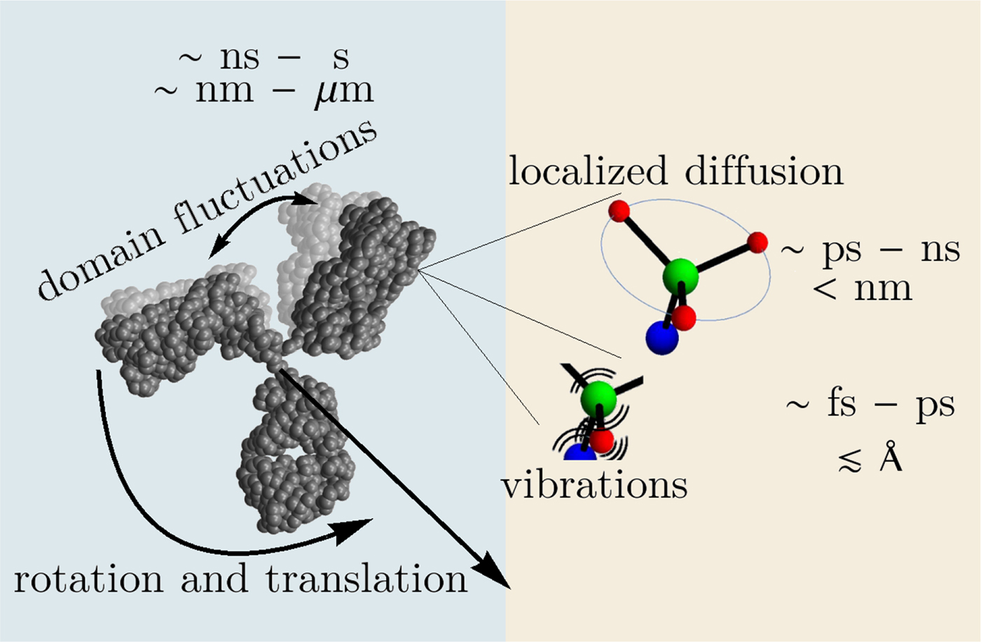
In the following, we outline four classes of dynamical processes occurring in proteins, from the largest supramolecular length scale to the smallest atomic length scale of chemical groups, all of which are linked and can contribute to the protein function (Henzler-Wildman et al., Reference Henzler-Wildman, Lei, Thai, Kerns, Karplus and Kern2007). A sketch representing these types of processes is shown in Fig. 1. We emphasize already at this point that different techniques with different experimental resolution address potentially very different dynamical regimes, all of which are relevant for a complete picture of these complex systems at the interface of physics, biology and chemistry (Sakai et al., Reference Sakai, Alba-Simionesco and Chen2011; Khodadadi and Sokolov, Reference Khodadadi and Sokolov2017; Narayanan et al., Reference Narayanan, Wacklin, Konovalov and Lund2017).
Sketch of different types of protein dynamics. Left: The rotation and translation of the entire protein occurs on timescales of nanoseconds to seconds and lengthscales from nanometers to micrometers. Domain fluctuations occur on timescales of several nanoseconds to milliseconds with amplitudes from some Ångströms to about a nanometer. Right: Localized and confined diffusive relaxations occurring on a timescale of picoseconds to nanoseconds and a subnanometer length scale, as well as vibrations occurring on the femto- to pico-second timescale with amplitudes up to a few Ångströms are depicted. The IgG protein (Harris et al., Reference Harris, Larson, Hasel and McPherson1997) was rendered using Mathematica (Wolfram Research, Inc.) and the figure was produced using Mathematica (Wolfram Research, Inc.) and Gimp (Spencer Kimball and the GIMP Development Team).
Diffusion of the entire protein
On the largest supramolecular scale, global diffusion occurs in two types: (1) gradients and fluctuations in the protein concentration are relaxed by collective diffusion, which depends on the protein–protein interactions and allows to connect to thermodynamic quantities of protein solutions. (2) Self-diffusion or synonymously tracer-diffusion of the entire molecule depends on the surrounding medium with possible obstacles. Theoretically, these two types of diffusion are defined by their respective correlation functions (see Eqs. (15) and (16)). Experimentally, the two types of diffusion are determined by the specific methods that access them separately.
As for all diffusive processes without global confinement, time and length scales are directly related via the diffusion coefficient D: relaxations on a length scale L occur on the timescale τ D = L 2/(4π 2D) = 1/(Dq 2) with the wavevector q = (2π)/L. In a real system with various environmental factors such as e.g. other macromolecules serving as ‘obstacles’, diffusion becomes a scale-dependent process. The mean-square displacement (MSD)
 $$\langle{{\rm \Delta} r^2} \rangle = 6D\lpar t \rpar t^\alpha $$
typically changes from simple diffusive behavior (α = 1) at nanosecond timescales to a crossover regime with apparent anomalous subdiffusion (α < 1) at microsecond timescales, and may recover another simple diffusive regime at much longer timescales (Höfling and Franosch, Reference Höfling and Franosch2013) (see Fig. 2).
Sketch of the diffusive MSD W(t) as a function of time. For very short times, W(t) ~ t 2. For t B < t < t I,  $W\lpar t \rpar \sim D_{\rm s}^{\lpar {\rm s} \rpar } \,t$, and for t ≫ t I, $W\lpar t \rpar \sim D_l^{\lpar {\rm s} \rpar } \,t$. τ I is the typical interaction time, i.e. the time on which proteins collide.

A possible and remarkably productive framework to describe the global center-of-mass protein diffusion in liquid solutions is provided by colloid physics (see section ‘Diffusion of the entire protein’), which predicts a short-time regime on which only hydrodynamic interactions induce a simple diffusive behavior (see Fig. 2). Beyond a so-called interaction time τ I, often approximated with the time needed for a protein to diffuse to a distance equal to its own radius, collisions of the proteins with obstacles increasingly slow down the motion, giving rise to subdiffusive behavior. At very long times, the interparticle interactions average out, and a simple diffusive long-time regime is recovered. Indeed, a rough estimate for the interaction timescale for a globular protein under conditions of macromolecular crowding yields 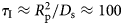 $\tau _{\rm I}\approx R_{\rm p}^2 /D_{\rm s}\approx 100$ ns (R p ~ 2.5 nm protein radius, D s ~ 7 Å2 ns−1 short-time diffusion coefficient), consistent with the overall observations.
On the length scale of the protein size, rotational diffusion significantly contributes to the entire-molecule motion. Depending on the experimental technique, rotational diffusion can contribute a constant offset in the observed relaxation coefficient (e.g. dynamic light scattering (DLS); Berne and Pecora, Reference Berne and Pecora2000), appear as an apparent simple diffusion accounting for rotations and translations together (e.g. QENS, see section ‘Diffusion of the entire protein’ for details), or also be accessed directly (e.g. relaxometric nuclear magnetic resonance (NMR); Korzhnev et al., Reference Korzhnev, Billeter, Arseniev and Orekhov2001; d'Auvergne and Gooley, Reference d'Auvergne and Gooley2008; Bouchoux et al., Reference Bouchoux, Schorr, Daffé, Cambert, Gesan-Guiziou and Mariette2012; Roos et al., Reference Roos, Ott, Hofmann, Link, Roössler, Balbach, Krushelnitsky and Saalwächter2016).
Despite numerous positive results, the small size and softness of globular proteins poses a challenge for the application of colloidal concepts and theories in order to describe their translational and rotational diffusion in aqueous solution. In this context, the class of intrinsically disordered proteins (IDPs) as well as unfolded protein chains provides an interesting test case, how far colloidal concepts can be merged with polymer descriptions to account for the complex dynamics of unfolded structures. Moreover, the inhomogeneous surface charge pattern of proteins and their tendency, under certain conditions, to form clusters constitutes an additional challenge to colloid physics.
Recently, mutual inspiration from protein studies and colloid physics has led to the remarkably successful development and application of the theory of ‘patchy colloids’ for the interpretation of a number of experimental observations (Gögelein et al., Reference Gögelein, Nägele, Tuinier, Gibaud, Stradner and Schurtenberger2008; Whitelam, Reference Whitelam2010; Bianchi et al., Reference Bianchi, Blaak and Likos2011; Roosen-Runge et al., Reference Roosen-Runge, Zhang, Schreiber and Roth2014). Thus, the study of proteins in solution under different conditions is ideal for testing and refining such theories, and is promising for smart engineering of self-assembling nano-particles and crystallization pathways.
Fluctuations of protein domains
The largest internal motions concern collective fluctuations of domains relative to each other. These motions, which also depend on the fluctuations of bulk solvent (Frauenfelder et al., Reference Frauenfelder, Chen, Berendzen, Fenimore, Jansson, McMahon, Stroe, Swenson and Young2009), can occur on rather long timescales from tens of nanoseconds to milliseconds (Henzler-Wildman et al., Reference Henzler-Wildman, Lei, Thai, Kerns, Karplus and Kern2007; Biehl et al., Reference Biehl, Monkenbusch and Richter2011). Interdomain motions can be essential to protein function, e.g. in the case of cleft-opening around catalytic centers (Biehl et al., Reference Biehl, Hoffmann, Monkenbusch, Falus, Prévost, Merkel and Richter2008). Furthermore, an understanding of these collective modes is important to understand un- and re-folding of proteins.
Conceptually, the interdomain motions have been linked back to overdamped low-frequency normal modes of the protein, and also resemble principal components of dynamics from computer simulations. The underlying idea is in these cases that the coordinate of the mode diffuses under an overall harmonic potential, corresponding to an Ornstein–Uhlenbeck process (Kneller, Reference Kneller2000). Finally, as one interesting experimental signature of different modes besides the relaxation constant Γ, the motional Fourier amplitude has been considered, and can be indeed used to describe experimental data (for details see section ‘Large-scale and domain motions’).
Localized and confined diffusive relaxations
On smaller scales of several Ångströms within the protein, motions can be disentangled into local fluctuations of the backbone, and strongly confined diffusion of the side-chains fixed at the backbone anchor point and motionally restricted by neighboring side-chains. On the atomic scale of Ångström, diffusive rotations and jump-like reorientations of chemical and functional groups such as methyl represent the fastest processes to diffusive protein dynamics.
Since a disentanglement of these motions is experimentally challenging, information on the motion of individual atoms can be obtained e.g. using two effective quantities accessible in experiments. First, the relaxation constant, often modeled as
 $${\rm \Gamma} \lpar q \rpar = \displaystyle{{Dq^2} \over {1 + D\tau q^2}},$$
provides insights into the overall diffusivity D of the atom as well as, from the q dependence, the motional character, i.e. continuous (τ = 0) or jump-like (τ > 0) motion. Second, the degree of confinement on a length scale L = 2π/q results in a change of the amplitude of the relaxations Γ(q) as a function of q, and provides interesting insight into the local geometric confinement of the atom motion (for details see section ‘Localized internal dynamics’).
Vibrational dynamics
On still faster timescales of femto- to pico-seconds and length scales of Ångströms and below, collective vibrational excitations of the protein occur as well as vibrations of individual chemical bonds in the protein. Employing various techniques, protein vibrations have been successfully studied to e.g. address redox-dependent properties (Chin et al., Reference Chin, Jimenez and Romesberg2002), pressure response (Lerbret et al., Reference Lerbret, Hdoux, Annighfer and Bellissent-Funel2013), determine cellular death (Verrier et al., Reference Verrier, Notingher, Polak and Hench2004) and study motions of the heme complex (Zhu et al., Reference Zhu, Sage and Champion1994; Levantino et al., Reference Levantino, Lemke, Schiro, Glownia, Cupane and Cammarata2015). These phenomena in the true inelastic regime are related to the so-called Boson peak in proteins and hydration water (Kataoka et al., Reference Kataoka, Kamikubo, Yunoki, Tokunaga, Kanaya, Izumi and Shibata1999b; Leyser et al., Reference Leyser, Doster and Diehl1999; Tarek and Tobias, Reference Tarek and Tobias2002; Roh et al., Reference Roh, Curtis, Azzam, Novikov, Peral, Chowdhuri, Gregory and Sokolov2006; Lerbret et al., Reference Lerbret, Hdoux, Annighfer and Bellissent-Funel2013; Khodadadi and Sokolov, Reference Khodadadi and Sokolov2017).
We do not further consider such vibrational motions in this review, because they appear less specific to aspects of protein dynamics in solution. For further details, we refer the reader to other reviews covering protein vibrations from the perspective of various specific techniques (Vogel and Siebert, Reference Vogel and Siebert2000; Parak, Reference Parak2003a; Nibbering et al., Reference Nibbering, Fidder and Pines2005; Vural et al., Reference Vural, Hu, Lindner, Jain, Miao, Cheng, Liu, Hong and Smith2017).
Overview: techniques addressing protein dynamics
The dynamical hierarchy of protein dynamics implies that a broad range of time and length scales has to be accessed to comprehensively describe the motions of proteins and their subunits. In this context, individual experimental techniques address specific windows of experimental scales, and contribute to an overall picture of protein dynamics (see Table 1 for a brief comparison). Ideally, such techniques should be non-invasive, efficient and should require the least possible interpretation. In this section, we outline common techniques for the study of protein dynamics and put them in a context regarding the accessed scales as well as other advantages and limitations.
Comparison between several techniques in the context of dynamics of proteins in solution

XPCS, X-ray photon correlation spectroscopy; TRXS, time-resolved X-ray scattering; TOF, neutron time-of-flight spectroscopy; NBS, neutron backscattering spectroscopy; NSE, neutron spin echo spectroscopy; NMR, nuclear magnetic resonance (for advanced techniques see text); PFG-NMR, pulsed-field gradient NMR; Diel. and THz spectroscopy: dielectrical and terahertz spectroscopy; FCS, fluorescence correlation spectroscopy; FRAP, fluorescence recovery after photobleaching; FRET, Förster resonance energy transfer.
Scattering techniques
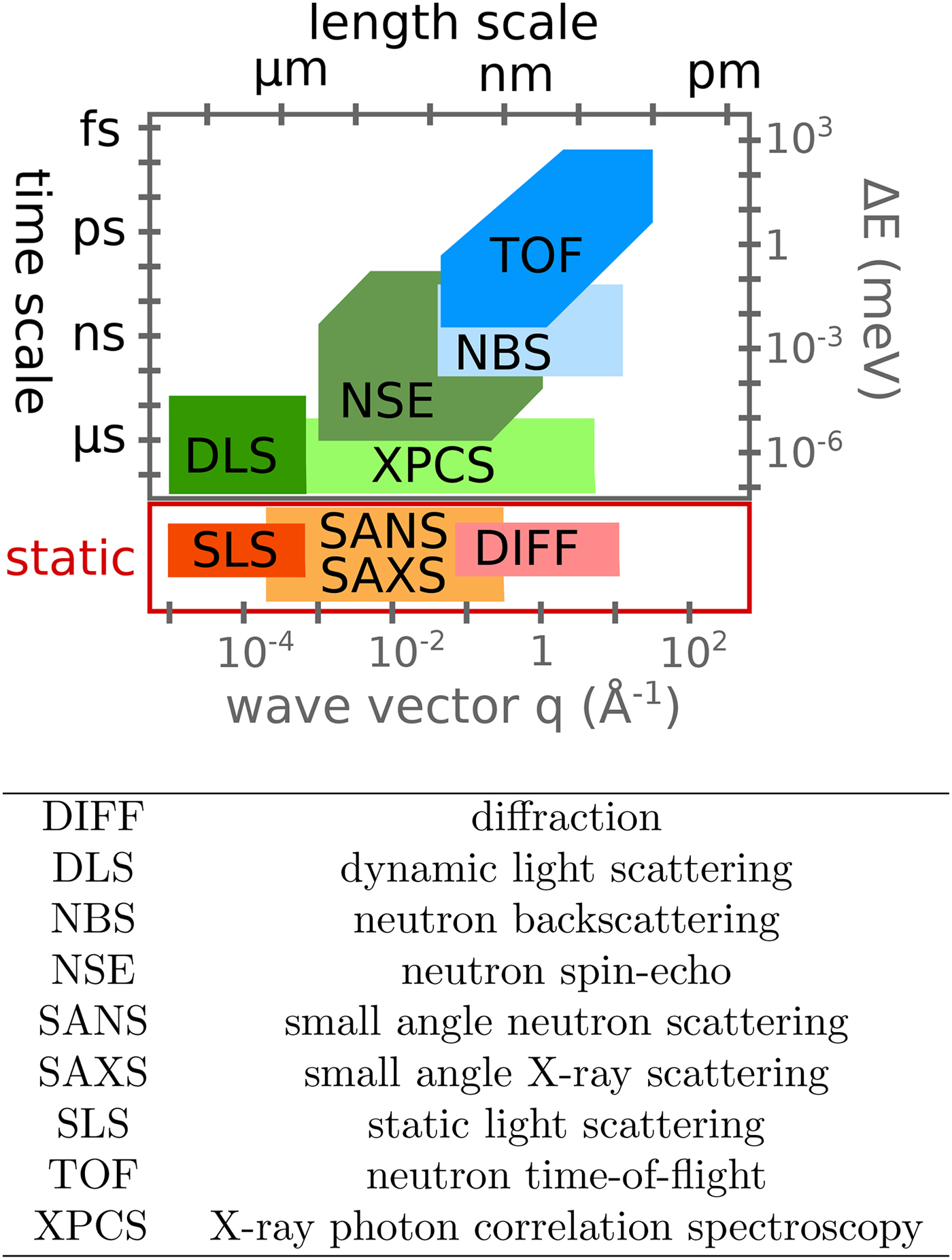
Various probe particles may be used by scattering experiments, such as protons, electrons, He-atoms, photons or neutrons. For biological matter including proteins, photons and neutrons constitute the most obvious choice, because they can be tuned to energy ranges where they cause little or no damage and access intermolecular length scales. Furthermore, they can penetrate bulk matter including solvents. In the case of photons, the hard X-ray regime causes sufficiently little damage on the required measurement times due to the weak interaction of high-energy photons with biological matter. In the case of neutrons, the cold and thermal energy range from ~2 to 25 meV is perfectly suitable, since these energies well below the energies of chemical bonds do not cause any damage at all. The simultaneous access to information on well-defined time- and length scales (Fig. 3) makes scattering techniques a very valuable tool to study dynamics.
Accessible length- and time-scales of typical scattering techniques.
Scattering techniques provide three different modes how dynamics can be studied. Importantly, all of these include a clear notion of both the time and length scales on which dynamics occurs. First, dynamics can be studied through changes of the probe particle energy during the scattering event in the sample, as realized in neutron spectroscopy. In this context, cold or thermal neutrons allow for an unparalleled accuracy in defining the energy transfer due to their low absolute kinetic energies (on the order of 10 meV) compared with X-ray photons (on the order of 10 keV). Second, time-correlation spectroscopy can access the intensity fluctuations in the scattered wave field of a coherently illuminated sample, which is linked to underlying dynamical processes causing fluctuating phase shifts in the scattered radiation (Dierker et al., Reference Dierker, Pindak, Fleming, Robinson and Berman1995; Thurn-Albrecht et al., Reference Thurn-Albrecht, Steffen, Patkowski, Meier, Fischer, Grübel and Abernathy1996; Seydel et al., Reference Seydel, Madsen, Tolan, Grübel and Press2001; Grübel et al., Reference Grübel, Madsen, Robert, Borsali and Pecora2008; Sun et al., Reference Sun, Zhu, Song, Decker, Sutton, Ludwig, Roseker, Grübel, Hruszkewycz, Stephenson, Fuoss and Robert2017; Roseker et al., Reference Roseker, Hruszkewycz, Lehmkühler, Walther, Schulte-Schrepping, Lee, Osaka, Strüder, Hartmann, Sikorski, Song, Robert, Fuoss, Sutton, Stephenson and Grübel2018). Third, scattering profiles at a given time lag from a trigger signal in pump–probe time-resolved setups can be compared with obtained information on changes in the sample (Cho et al., Reference Cho, Dashdorj, Schotte, Graber, Henning and Anfinrud2010; Lima et al., Reference Lima, Milne, Amarasinghe, Rittmann-Frank, Veen, Reinhard, Pham, Karlsson, Johnson, Grolimund, Borca, Huthwelker, Janousch, van Mourik, Abela and Chergui2011; Navirian et al., Reference Navirian, Herzog, Goldshteyn, Leitenberger, Vrejoiu, Khakhulin, Wulff, Shayduk, Gaal and Bargheer2011; Kim et al., Reference Kim, Lee, Choi, Kim, van Wilderen, Guerin, Kim, Jung, Yang, Kim, Wulff, van Thor and Ihee2012b, Reference Kim, Kim, Kim and Ihee2015).
Neutron spectroscopy
In most cases relevant for biological studies, neutrons with Ångström wavelengths can be considered as classical particles that during the scattering process exchange momentum and energy with the sample. By measuring these changes, conclusions on the dynamics and structure in the sample can be drawn. Depending on the specific realization (see sections ‘Quasi-elastic neutron scattering theory’ and ‘Experimental techniques’ for details), timescales ranging from pico- to hundreds of nano seconds can be addressed on length scales ranging from Ångströms to several nanometers.
The simultaneous collection of spatial and temporal information as well as the inherent property of neutron spectroscopy to record ensemble averages allows a robust modeling of the statistical and motional characteristics of the underlying dynamical processes.
Neutron spectroscopy is an established technique to study systems of soft and biological matter (Fitter et al., Reference Fitter, Gutberlet and Katsaras2006; Sakai and Arbe, Reference Sakai and Arbe2009; Hoffmann, Reference Hoffmann2014), and due to the accessible time and length scales in particular suitable for protein dynamics (see section ‘Results’ for a comprehensive review). Using neutron spectroscopy, the full hierarchy of protein dynamics can be accessed, including global diffusion, inter-domain motions and local diffusive dynamics.
Photon correlation spectroscopy: dynamic light scattering (DLS) and X-ray photon correlation spectroscopy (XPCS)
Photon correlation spectroscopy is based on coherently illuminating a macroscopically large volume in the sample by a photon beam, which ranges from 100 to 1000 cubic micrometers at synchrotron sources up to the entire sample volume (~mm3) at laser sources for both visible light and X-ray photons.
In photon correlation spectroscopy, information on the collective dynamics inside the sample is accessed via the temporal fluctuations of the speckle pattern scattered from the coherently illuminated volume. While the timescale is thus set by the read-out frequency and the stability of the system, the length scale is related to the scattering vector at which the so-called speckle is observed.
DLS is probably the most frequently used lab-based technique to obtain information on diffusional properties in soft matter (Dhont, Reference Dhont1996; Murphy, Reference Murphy1997; Berne and Pecora, Reference Berne and Pecora2000; Gun'ko et al., Reference Gun'ko, Klyueva, Levchuk and Leboda2003; Scheffold and Cerbino, Reference Scheffold and Cerbino2007; Schmitz, Reference Schmitz2012; Phillies, Reference Phillies2016). Given the long history of several decades and the ubiquitous use also in protein science, a complete coverage of DLS results is beyond the scope of this review, and we only briefly mention a few case studies. Based on the measured translational collective (or gradient) diffusion coefficients on timescales of typically microseconds and length scales of micrometers, inter alia protein interactions (Phillies et al., Reference Phillies, Benedek and Mazer1976; Muschol and Rosenberger, Reference Muschol and Rosenberger1995; Kuehner et al., Reference Kuehner, Heyer, Rämsch, Fornefeld, Blanch and Prausnitz1997; Heinen et al., Reference Heinen, Zanini, Roosen-Runge, Fedunova, Zhang, Hennig, Seydel, Schweins, Sztucki, Antalik, Schreiber and Nägele2012), protein assemblies (Schurtenberger and Augusteyn, Reference Schurtenberger and Augusteyn1991; Shen et al., Reference Shen, Scott, Merchant and Murphy1993; Ferré-D'Amaré and Burley, Reference Ferré-D'Amaré and Burley1994; Piazza, Reference Piazza2004; Soraruf et al., Reference Soraruf, Roosen-Runge, Grimaldo, Zanini, Schweins, Seydel, Zhang, Roth, Oettel and Schreiber2014) and unfolding and denaturation (Baussay et al., Reference Baussay, Bon, Nicolai, Durand and Busnel2004; Jachimska et al., Reference Jachimska, Wasilewska and Adamczyk2008) have been addressed. Using depolarized DLS, also rotational self-diffusion has been accessed (Dubin et al., Reference Dubin, Clark and Benedek1971; Berne and Pecora, Reference Berne and Pecora2000).
XPCS is a synchrotron-based technique, accessing length scales from the atomic scale up to a few micrometers (Grübel et al., Reference Grübel, Madsen, Robert, Borsali and Pecora2008; Leheny, Reference Leheny2012; Möller et al., Reference Möller, Chushkin, Prévost and Narayanan2016). So far, it has only been used tentatively for protein dynamics because of the prevailing challenge of radiation damage (Vodnala et al., Reference Vodnala, Karunaratne, Lurio, Thurston, Vega, Gaillard, Narayanan, Sandy, Zhang, Dufresne, Foffi, Grybos, Kmon, Maj and Szczygiel2018), although XPCS could provide a unique time and length scale window for collective dynamics, and there may be ways to circumvent the problems (Verwohlt et al., Reference Verwohlt, Reiser, Randolph, Matic, Medina, Madsen, Sprung, Zozulya and Gutt2018). The advent of free-electron lasers provides further promising opportunities for X-ray based techniques, such as X-ray speckle visibility studies using a single bunch and a delay line with variable lag time.
Time resolved X-ray solution scattering (TRXS)
When specific time-dependent processes in proteins can be triggered, e.g. by photoactivation or changes of temperature and other environmental factors, the subsequent kinetics of changes of the protein structure can be followed by collecting scattering profiles at multiple suitably chosen lag times (Ihee et al., Reference Ihee, Wulff, Kim and Adachi2010). For slower processes on timescales longer than several microseconds such as assembly of virus capsids, crystal nucleation, as well as protein folding, these profiles can be collected on one identical sample, or in stopped-flow or rapid fluid mixing setups (Pollack et al., Reference Pollack, Tate, Finnefrock, Kalidas, Trotter, Darnton, Lurio, Austin, Batt, Gruner and Mochrie2001; Svergun and Koch, Reference Svergun and Koch2003; Kirby and Cowieson, Reference Kirby and Cowieson2014; Sauter et al., Reference Sauter, Roosen-Runge, Zhang, Lotze, Jacobs and Schreiber2015).
Faster processes on timescales below a few microseconds require pump–probe setups, in which the trigger signal is followed by the X-ray pulse after a defined lag time. The duration of the X-ray pulse sets the minimum accessible timescales to roughly 100 ps at third-generation synchrotron sources and clearly below 1 ps for X-ray free-electron lasers (Ihee et al., Reference Ihee, Wulff, Kim and Adachi2010; Kirby and Cowieson, Reference Kirby and Cowieson2014).
By these techniques, photo-induced protein dynamics on picosecond timescales could be addressed e.g. in hemoglobin (Hb) (Cammarata et al., Reference Cammarata, Levantino, Schotte, Anfinrud, Ewald, Choi, Cupane, Wulff and Ihee2008; Kim et al., Reference Kim, Muniyappan, Oang, Kim, Nozawa, Sato, Koshihara, Henning, Kosheleva, Ki, Kim, Kim, Kim, Adachi and Ihee2012a, Reference Kim, Kim, Kim and Ihee2015), myoglobin (Mb) (Ahn et al., Reference Ahn, Kim, Kim, Kim and Ihee2009; Cho et al., Reference Cho, Dashdorj, Schotte, Graber, Henning and Anfinrud2010), photoactive yellow protein (Kim et al., Reference Kim, Kim, Kim and Ihee2015), proton pumps (Andersson et al., Reference Andersson, Malmerberg, Westenhoff, Katona, Cammarata, Wöri, Johansson, Ewald, Eklund, Wulff, Davidsson and Neutze2009) and a photosynthetic reaction center (Arnlund et al., Reference Arnlund, Johansson, Wickstrand, Barty, Williams, Malmerberg, Davidsson, Milathianaki, DePonte, Shoeman, Wang, James, Katona, Westenhoff, White, Aquila, Bari, Berntsen, Bogan, van Driel, Doak, Kjaer, Frank, Fromme, Grotjohann, Henning, Hunter, Kirian, Kosheleva, Kupitz, Liang, Martin, Nielsen, Messerschmidt, Seibert, Sjohamn, Stellato, Weierstall, Zatsepin, Spence, Fromme, Schlichting, Boutet, Groenhof, Chapman and Neutze2014). Given the necessity of a trigger signal, the application of this ultra-fast TRXS is limited to specific cases, and usually requires additional molecular modeling to interpret the data.
Fluorescence techniques
Fluorescence-based techniques provide a well-established, lab-based access to several aspects of protein dynamics, and are frequently used to obtain information on in-vivo biological systems (Lippincott-Schwartz et al., Reference Lippincott-Schwartz, Snapp and Kenworthy2001; Rivas and Minton, Reference Rivas and Minton2016).
The required insertion of a fluorescence marker can be both advantageous, since it provides opportunities to target the property in question, and disadvantageous, since the solution behavior of proteins might be altered significantly (Quinn et al., Reference Quinn, Gnan, James, Ninarello, Sciortino, Zaccarelli and McManus2015; Rivas and Minton, Reference Rivas and Minton2016).
While a thorough overview over this vivid research methodology is beyond the scope of this review, we briefly discuss main techniques, and refer the reader to review articles for further information (Lippincott-Schwartz et al., Reference Lippincott-Schwartz, Snapp and Kenworthy2001; Rivas and Minton, Reference Rivas and Minton2016).
Fluorescence recovery after photobleaching (FRAP)
The basic idea of FRAP is to bleach the fluorophores in a part of the sample, and then record how the fluorescence signal recovers in time, yielding the density of fresh intruders as the observable. The length scale of the accessed dynamics is set by the optical resolution and bleaching volume (typically around a few micrometers), whereas the timescale is limited by the scanning speed of the confocal microscope to timescales of several milliseconds. Multiple variants of FRAP differing e.g. in the geometry of the bleach volume have been exploited (Bancaud et al., Reference Bancaud, Huet, Rabut and Ellenberg2010). The achieved results include protein mobility, topology of cellular compartments and protein reaction dynamics (Lippincott-Schwartz et al., Reference Lippincott-Schwartz, Snapp and Kenworthy2001; Bancaud et al., Reference Bancaud, Huet, Rabut and Ellenberg2010; Fritzsche and Charras, Reference Fritzsche and Charras2015).
Fluorescence correlation spectroscopy (FCS)
In FCS, the correlation of the fluorescence intensity is used to obtain information on the diffusion time of molecules across the confocal volume (Lippincott-Schwartz et al., Reference Lippincott-Schwartz, Snapp and Kenworthy2001; Krichevsky and Bonnet, Reference Krichevsky and Bonnet2002). The accessible timescales start around several 100 ns, and are mainly determined by the deadtime of the photon counting detector and the subsequent hardware correlator. The length scales are directly given by the confocal volume, which usually is around a few μm3. Using the autocorrelation of single dyes, translational and rotational motions can be addressed (Lippincott-Schwartz et al., Reference Lippincott-Schwartz, Snapp and Kenworthy2001; Krichevsky and Bonnet, Reference Krichevsky and Bonnet2002; Di Rienzo et al., Reference Di Rienzo, Piazza, Gratton, Beltram and Cardarelli2014), while cross correlations of two dyes allow for a dynamical picture of binding and protein interaction (Lippincott-Schwartz et al., Reference Lippincott-Schwartz, Snapp and Kenworthy2001; Bacia et al., Reference Bacia, Kim and Schwille2006).
Förster resonance energy transfer (FRET)
The energy transfer between specific pairs of donor and acceptor dyes exhibits a strong distance dependence on the scale of a few nanometers, which allows for high-precision measurements of the distance between labeled sites by measuring the efficiency of the transfer (Deniz et al., Reference Deniz, Laurence, Dahan, Chemla, Schultz and Weiss2001; Lippincott-Schwartz et al., Reference Lippincott-Schwartz, Snapp and Kenworthy2001; Piston and Kremers, Reference Piston and Kremers2007; Roy et al., Reference Roy, Hohng and Ha2008). The fastest accessible timescales are set by the read-out frequency of the photon detector, while the longest timescales are limited by the time molecules stay in the confocal volume. Since this time is of the order of a few milliseconds for freely diffusing molecules, long-time processes can only be monitored when molecules are immobilized (Lippincott-Schwartz et al., Reference Lippincott-Schwartz, Snapp and Kenworthy2001; Roy et al., Reference Roy, Hohng and Ha2008).
The choice of the labeling dyes allows to fine-tune the sensitivity, and defines the type of possible experiment. Using two dyes on two molecules, intermolecular docking can be studied in time (Lippincott-Schwartz et al., Reference Lippincott-Schwartz, Snapp and Kenworthy2001; Piston and Kremers, Reference Piston and Kremers2007; Roy et al., Reference Roy, Hohng and Ha2008) as well as protein localizations in the cell (Sekar and Periasamy, Reference Sekar and Periasamy2003). Labeling two sites on a single molecule, folding dynamics under native and denaturing conditions can be studied (Nienhaus, Reference Nienhaus2006; Borgia et al., Reference Borgia, Williams and Clarke2008; Schuler and Eaton, Reference Schuler and Eaton2008; Ferreon and Deniz, Reference Ferreon and Deniz2011). While adding specificity to the obtained information, the attachment of dyes can also have severe drawbacks, since their effects on internal dynamics and intermolecular interactions might not be negligible (Sánchez-Rico et al., Reference Sánchez-Rico, Voith von Voithenberg, Warner, Lamb and Sattler2017).
Nuclear magnetic resonance (NMR) techniques
A multitude of NMR techniques exists and has been exploited to address protein dynamics and folding. We refer the reader to reviews from the last decade for a more detailed overview (Dosset et al., Reference Dosset, Hus, Blackledge and Marion2000; Ishima and Torchia, Reference Ishima and Torchia2000; Dyson and Wright, Reference Dyson and Wright2004; Blackledge, Reference Blackledge2005; Kay, Reference Kay2005; Boehr et al., Reference Boehr, Dyson and Wright2006; Mittermaier and Kay, Reference Mittermaier and Kay2009; Kleckner and Foster, Reference Kleckner and Foster2011; Krushelnitsky et al., Reference Krushelnitsky, Reichert and Saalwächter2013). Standard measurements of the spin relaxations in protein solutions are bound to timescales of pico- to nanoseconds due to the protein tumbling (Boehr et al., Reference Boehr, Dyson and Wright2006; Kleckner and Foster, Reference Kleckner and Foster2011; Krushelnitsky et al., Reference Krushelnitsky, Reichert and Saalwächter2013). A much broader range of timescales up to seconds can be accessed using more specialized NMR techniques, such as e.g. residual dipolar couplings, exchange spectroscopy and real-time NMR (Blackledge, Reference Blackledge2005; Boehr et al., Reference Boehr, Dyson and Wright2006; Kleckner and Foster, Reference Kleckner and Foster2011). While a full hierarchy of timescales is accessible, spatial information on dynamical processes can only be inferred through modeling when using NMR, with few exceptions (see below).
For most of these techniques, labeling with specific isotopes such as 13C and 15N is used, and also allows for site-specific information on protein dynamics in a non-invasive way.
In pulsed-field gradient NMR (PFG-NMR) (Price, Reference Price1997) or variants such as diffusion ordered spectroscopy (Johnson, Reference Johnson1999), the spin echo after at least two pulsed field gradients allows to obtain information on the molecular translational mobility, since displacement of the protein results in a varied phase shift. Technically, the timescale is set by the pulse separation usually on the order of several milliseconds. Practically, the spin–spin relaxation provides an upper limit for the accessible timescale. Importantly, the length scale can be independently set via the gradient (within certain technical limits), which allows to obtain information on diffusion coefficient and confinement geometry (Price, Reference Price1997).
Using translational self-diffusion coefficients, PFG-NMR allows for systematic study of numerous aspects of protein dynamics (Price, Reference Price2000), such as aggregation behavior (Price et al., Reference Price, Tsuchiya and Arata1999), unfolding (Wilkins et al., Reference Wilkins, Grimshaw, Receveur, Dobson, Jones and Smith1999) or effects of protein concentration (Le Bon et al., Reference Le Bon, Nicolai, Kuil and Hollander1999; Roos et al., Reference Roos, Link, Balbach, Krushelnitsky and Saalwächter2015, Reference Roos, Ott, Hofmann, Link, Roössler, Balbach, Krushelnitsky and Saalwächter2016).
Dielectric and terahertz spectroscopy
Dielectric spectroscopy has been used to obtain information on the dynamics of proteins in solution and, in particular, their hydration properties from the dielectric spectrum up to several gigahertz (Nandi et al., Reference Nandi, Bhattacharyya and Bagchi2000; Oleinikova et al., Reference Oleinikova, Sasisanker and Weingärtner2004; Cerveny et al., Reference Cerveny, Alegría and Colmenero2008; Frauenfelder et al., Reference Frauenfelder, Chen, Berendzen, Fenimore, Jansson, McMahon, Stroe, Swenson and Young2009; Fenimore et al., Reference Fenimore, Frauenfelder, Magazù, McMahon, Mezei, Migliardo, Young and Stroe2013; Nakanishi and Sokolov, Reference Nakanishi and Sokolov2015). Usually, the dielectric spectrum in protein solutions displays three main features, denoted as β, γ and δ dispersion, representing dielectric relaxation processes at well-separated timescales. While the technique is well-established, no general consensus of the physical origins of the dispersions has been found, and computer simulations and comparison with other techniques are needed for a conclusive assignment (Nakanishi and Sokolov, Reference Nakanishi and Sokolov2015).
While the β dispersion with relaxation times around tenths of nanoseconds can be assigned to protein tumbling, the γ dispersion on timescales of a few picoseconds is attributed to bulk water reorientations (Oleinikova et al., Reference Oleinikova, Sasisanker and Weingärtner2004). The origin of the bimodal δ dispersion at timescales of 100 ps to 1 ns is usually assigned to processes connected to the dynamics of hydration water (Nandi et al., Reference Nandi, Bhattacharyya and Bagchi2000; Oleinikova et al., Reference Oleinikova, Sasisanker and Weingärtner2004).
Improvements in experimental techniques allowed the extension into the terahertz regime, corresponding to timescales down to around 1 ps (Markelz et al., Reference Markelz, Roitberg and Heilweil2000; Jepsen et al., Reference Jepsen, Cooke and Koch2011; Falconer and Markelz, Reference Falconer and Markelz2012; Bellissent-Funel et al., Reference Bellissent-Funel, Hassanali, Havenith, Henchman, Pohl, Sterpone, van der Spoel, Xu and Garcia2016). In connection with theoretical modeling, the changes in absorbance have been linked to changes in the vibrational states of proteins (Castro-Camus and Johnston, Reference Castro-Camus and Johnston2008; Acbas et al., Reference Acbas, Niessen, Snell and Markelz2014), and solvation effects on proteins (Markelz et al., Reference Markelz, Roitberg and Heilweil2000; Xu et al., Reference Xu, Plaxco and Allen2006; Ebbinghaus et al., Reference Ebbinghaus, Kim, Heyden, Yu, Gruebele, Leitner and Havenith2008).
Molecular dynamics simulations
Molecular dynamics (MD) simulations complement experimental methods and modeling. The interpretation of experimental data with the help of MD simulations has evolved into a very large field (e.g. Smith, Reference Smith1991; Daniel et al., Reference Daniel, Dunn, Finney and Smith2003; Sakai and Arbe, Reference Sakai and Arbe2009; Smith et al., Reference Smith, Tan, Petridis and Hong2018) beyond the scope of this review. The comparison of results from simulated atom trajectories with experimental scattering functions has been achieved using software packages such as nMOLDYN (Kneller et al., Reference Kneller, Keiner, Kneller and Schiller1995; Róg et al., Reference Róg, Murzyn, Hinsen and Kneller2003) or MDANSE (Goret et al., Reference Goret, Aoun and Pellegrini2017). To this effect, these software packages calculate the simulated scattering functions from the computed trajectories, and the possibility to selectively investigate for instance only some molecular groups contributes to the advantages of the simulation approach. To some extent, the simulation approach can be an alternative to the use of models outlined in the ‘Modeling and analysis’ section, especially for the interpretation of increasingly complex systems (Kneller, Reference Kneller2005; Sakai and Arbe, Reference Sakai and Arbe2009).
Other techniques on protein dynamics
Multiple other techniques have been used to study different aspects of the dynamics of proteins, which are beyond the scope of this review, and should only be mentioned briefly with key references.
Also exploiting magnetic resonance, but different from NMR, electron spin resonance has to be mentioned, which requires an unpaired electron spin for detection. It can also serve as a microscopic probe for the dynamics and kinetics in situ (Steinhoff et al., Reference Steinhoff, Mollaaghababa, Altenbach, Hideg, Krebs, Khorana and Hubbell1994; Klose et al., Reference Klose, Voskoboynikova, Orban-Glass, Rickert, Engelhard, Klare and Steinhoff2014; Beutel et al., Reference Beutel, Roder, Birkholz, Rickert, Steinhoff, Grzybek, Coskun and Piehler2015; Dunkel et al., Reference Dunkel, Pulagam, Steinhoff and Klare2015; Matthies et al., Reference Matthies, Glinka, Theiling, Hideg and Steinhoff2016).
As a classical tool to study vibrational dynamics we should mention infrared (IR) and Raman spectroscopy, which can also be performed in a time-dependent way to investigate various aspects of protein dynamics and kinetics of transformations (Arrondo and Goñi, Reference Arrondo and Goñi1999; Zanni and Hochstrasser, Reference Zanni and Hochstrasser2001; Schweitzer-Stenner, Reference Schweitzer-Stenner2005; Garczarek and Gerwert, Reference Garczarek and Gerwert2006; Kolano et al., Reference Kolano, Helbing, Kozinski, Sander and Hamm2006; Barth, Reference Barth2007; Kong and Yu, Reference Kong and Yu2007; Balakrishnan et al., Reference Balakrishnan, Weeks, Ibrahim, Soldatova and Spiro2008; Fayer, Reference Fayer2009; Kim and Hochstrasser, Reference Kim and Hochstrasser2009; Kötting and Gerwert, Reference Kötting and Gerwert2015; Kuhne et al., Reference Kuhne, Eisenhauer, Ritter, Hegemann, Gerwert and Bartl2015; López-Peña et al., Reference López-Peña, Leigh, Schlamadinger and Kim2015; Schröter et al., Reference Schröter, Mann, Kötting and Gerwert2015).
High-speed atomic force microscopy (AFM) allows to study protein dynamics sticking to a surface on timescales of a few milliseconds with nanometer-resolution (Ando et al., Reference Ando, Kodera, Takai, Maruyama, Saito and Toda2001; Casuso et al., Reference Casuso, Rico and Scheuring2011; Katan and Dekker, Reference Katan and Dekker2011).
Single-molecule force spectroscopy using AFM, optical or magnetic tweezers accesses the folding dynamics in response to severe mechanical stresses (Viani et al., Reference Viani, Schäffer, Chand, Rief, Gaub and Hansma1999; Zhuang and Rief, Reference Zhuang and Rief2003; Borgia et al., Reference Borgia, Williams and Clarke2008; Neuman and Nagy, Reference Neuman and Nagy2008; Ferreon and Deniz, Reference Ferreon and Deniz2011).
Very recent developments in super-resolution microscopy allow for the tracking of single fluorescence-labeled molecules on length scales of several nanometers down to timescales of several milliseconds, such as the dynamics of the cytoskeleton, chromatin-binding and freely diffusing proteins in the cell (Schneider et al., Reference Schneider, Zahn, Maglione, Sigrist, Marquard, Chojnacki, Krausslich, Sahl, Engelhardt and Hell2015; Balzarotti et al., Reference Balzarotti, Eilers, Gwosch, Gynnå, Westphal, Stefani, Elf and Hell2016; Basu et al., Reference Basu, Tan, Taylor, Laue, Lee and Leake2016; Finkenstaedt-Quinn et al., Reference Finkenstaedt-Quinn, Qiu, Shin and Haynes2016; Nienhaus and Nienhaus, Reference Nienhaus and Nienhaus2016).
Time-resolved Laue X-ray crystallography achieved high-resolution information on photo-activated protein dynamics in the crystalline state (Wulff et al., Reference Wulff, Schotte, Naylor, Bourgeois, Moffat and Mourou1997; Srajer et al., Reference Srajer, Ren, Teng, Schmidt, Ursby, Bourgeois, Pradervand, Schildkamp, Wulff and Moffat2001; Schotte et al., Reference Schotte, Lim, Jackson, Smirnov, Soman, Olson, Phillips, Wulff and Anfinrud2003, Reference Schotte, Cho, Kaila, Kamikubo, Dashdorj, Henry, Graber, Henning, Wulff, Hummer, Kataoka and Anfinrud2012; Aquila et al., Reference Aquila, Hunter, Doak, Kirian, Fromme, White, Andreasson, Arnlund, Bajt, Barends, Barthelmess, Bogan, Bostedt, Bottin, Bozek, Caleman, Coppola, Davidsson, DePonte, Elser, Epp, Erk, Fleckenstein, Foucar, Frank, Fromme, Graafsma, Grotjohann, Gumprecht, Hajdu, Hampton, Hartmann, Hartmann, Hau-Riege, Hauser, Hirsemann, Holl, Holton, Hömke, Johansson, Kimmel, Kassemeyer, Krasniqi, Kühnel, Liang, Lomb, Malmerberg, Marchesini, Martin, Maia, Messerschmidt, Nass, Reich, Neutze, Rolles, Rudek, Rudenko, Schlichting, Schmidt, Schmidt, Schulz, Seibert, Shoeman, Sierra, Soltau, Starodub, Stellato, Stern, Strüder, Timneanu, Ullrich, Wang, Williams, Weidenspointner, Weierstall, Wunderer, Barty, Spence and Chapman2012). Temperature dependencies of protein crystallography have been used to address spatial information on dynamical flexibility in the protein (Frauenfelder et al., Reference Frauenfelder, Petsko and Tsernoglou1979).
In special cases of proteins containing Mössbauer-active isotopes such as 57Fe, Mössbauer spectroscopy has been used to provide information on the mean-square displacement in proteins (Frauenfelder et al., Reference Frauenfelder, Parak and Young1988, Reference Frauenfelder, Chen, Berendzen, Fenimore, Jansson, McMahon, Stroe, Swenson and Young2009; Parak, Reference Parak2003a, Reference Parakb; Fenimore et al., Reference Fenimore, Frauenfelder, Magazù, McMahon, Mezei, Migliardo, Young and Stroe2013).
In the context of dynamics, we shall also mention rheology-related techniques, although they are slightly different in nature than some of the other techniques. For a background on rheology, we refer to Mewis and Wagner (Reference Mewis and Wagner2012) and Zhang and Liu (Reference Zhang and Liu2017).
Overview: complementarity of techniques
Protein dynamics occurs on broad and hierarchical timescales ranging from picoseconds up to seconds, and length scales between Ångströms and several nanometers (for internal dynamics) or even millimeters (for long-range diffusion). Revisiting the different characteristics of the experimental techniques (Table 1), the necessity for complementary studies on protein dynamics becomes clear. NMR, dielectric and THz spectroscopy provide a broad range of timescales, but cannot be interpreted without the knowledge of the spatial distribution of the underlying motions. A combination of scattering techniques, PFG-NMR and fluorescence techniques, in combination with computer simulations, can provide the missing information, although individual techniques are bound to smaller time windows.
While this review is centered around protein dynamics as seen by QENS, we aim to provide connections to the other techniques to put forward a more comprehensive and detailed picture of protein dynamics, and promote fruitful, mutual understanding in the scientific landscape studying it.
Principles of neutron spectroscopy
Quasi-elastic neutron scattering theory
In the following, a short introduction to the theory of neutron scattering will be given. For a more complete treatment of neutron scattering, the reader is invited to consult for instance the article by Schober (Reference Schober2014) and the text books by Squires (Reference Squires2012) and Bee (Reference Bee1988), on which this section is based.
Neutrons are spin-1/2 subatomic particles having a mass m ≃ 1.67 × 10⁻²⁷ kg, and carrying no net charge, but a magnetic dipole moment. Together with protons, they are usually found in atomic nuclei, where they are stable. Free neutrons, which can be produced by fission or spallation nuclear reactions, are unstable and decay to a proton, an electron and an antineutrino with a mean lifetime of about 15 min. Their energy after moderation is simply equal to their non-relativistic kinetic energy:
 $$E_{{\rm kin}} = \displaystyle{1 \over 2}\; m\,v^2 = \displaystyle{{\hbar ^2}{k^2} \over {2m}},$$
where the last equality follows from the wave-particle duality with the wavevector  ${\bf k} = (m/\hbar\!){\bf v}$ (Bee, Reference Bee1988).
A neutron interacts with the atomic nuclei in the sample and can either be absorbed or scattered. In the case of scattering, the neutron may change, in addition to its spin orientation, its energy and its wavevector. Two basic quantities can be thus measured in a scattering experiment, that is, the energy transfer
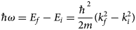 $$\hbar\!\omega = E_f-E_i = \displaystyle{{\hbar ^2} \over {2m}}\lpar {k_f^2 -k_i^2} \rpar $$
between the energy of the neutron before, E i, and after, E f, the scattering event, and the scattering vector
 $${\bf q} = {\bf k}_i - {\bf k}_f,$$
in addition to the magnetic polarization state. A schematic representation of a scattering event is depicted in Fig. 4. It should be noted that, for inelastic scattering,  $\hbar\!\omega \ne 0$ implies that |k i| ≠ |k f|.
Schematic representation of a scattering event. An incoming neutron with initial wavevector  ${\bf k}_i$ interacts with an atomic nucleus and is scattered at an angle 2θ. After the event, its wavevector is ${\bf k}_f$. The scattering vector ${\bf q}$ is defined as the difference between ${\bf k}_f$ and ${\bf k}_i$. Figure rendered using Mathematica (Wolfram Research, Inc.).

The neutron-nucleus scattering is characterized by the scattering length b tot = b + ib abs, which, for the thermal neutrons considered here, is independent of the neutron energy and can be a complex number. The imaginary part of b tot represents absorption, while the real part is related to scattering. For a repulsive neutron-nucleus potential, b is positive, while a negative and very large b indicates the imminent appearance of a bound state. Note that an attractive potential does not necessarily require a negative b (Squires, Reference Squires2012; Schober, Reference Schober2014).
Since b characterizes the interaction between a neutron and a nucleus, its value is different not only for different elements, but also for different isotopes and spin states. In general, a sample is composed of several atomic species i, all with a given b i. The coherent  $b_i^{{\rm coh}} $ and the incoherent $b_i^{{\rm inc}} $ scattering lengths of the i species are defined as the average of b i over isotopes and spin states
 $$b_i^{{\rm coh}} = \langle{b_i} \rangle $$
and as the mean square deviation of b i from 〈b i〉
 $$b_i^{{\rm inc}} = \left[ {\langle{b_i^2} \rangle -{\langle{b_i} \rangle}^2} \right] ^{1/2},$$
respectively (Bee, Reference Bee1988).
The scattering length can be related to the probability that a neutron with incident energy E i leaves the sample in the solid angle element dΩ about the direction Ω and with an energy transfer between  $\hbar\! \omega $ and $\hbar\! (\omega + {\rm d}\omega {\rm )}$, that is the double-differential cross-section
 $$\displaystyle{{\partial ^2\sigma _{\rm s}} \over {\partial {\rm \Omega} \partial E}} = \displaystyle{1 \over \hbar} \displaystyle{{\partial ^2\sigma _{\rm s}} \over {\partial {\rm \Omega} \partial \omega}}. $$
The integral over Ω and E of the double-differential cross-section is the scattering cross-section σ s. Let I 0 be the number of incoming neutrons per unit of time and area, then the number I s of scattering events per unit of time is given by
 $$I_{\rm s} = I_{\rm 0}\,\sigma _{\rm s} = I_0 {\mathop \int \nolimits} \,{\rm d}E\; {\mathop \int \nolimits} \,{\rm d\Omega} {\displaystyle{{\partial ^2\sigma _{\rm s}} \over {\partial {\rm \Omega} \partial E}}},$$
with
 $$\sigma _{\rm s} = \sigma _{{\rm inc}} + \sigma _{{\rm coh}} = 4\pi {\rm (}b_{{\rm inc}}^2 {\rm}+{\rm } b_{{\rm coh}}^2 {\rm )}{\rm.} $$
We note that, similar to the scattering cross-section in Eq. (9), an absorption cross-section can be defined such that
 $$I_{\rm a} = I_0\,b_{{\rm abs}}^2 = I_0\,\sigma _{\rm a} = I_0 {\mathop \int \nolimits} \,{\rm d}E\; {\mathop \int \nolimits} \,{\rm d\Omega} \;{\displaystyle{{\partial ^2\sigma _{\rm a}} \over {\partial {\rm \Omega} \partial E}}},$$
where I a denotes the number of absorption events per unit of time (Bee, Reference Bee1988).
In general, a sample can be composed of n different types of atoms such as H, D, and C. It can be shown that, in the absence of coupling between the values of the scattering lengths for different isotopes (i.e. independent averages), the double-differential scattering cross-section can be written as
 $$\displaystyle{{\partial ^2\sigma _{\rm s}} \over {\partial {\rm \Omega} \partial \omega}} = \left( {\displaystyle{{\partial^2\sigma_{\rm s}} \over {\partial {\rm \Omega} \partial \omega}}} \right)_{{\rm coh}} +\; \left( {\displaystyle{{\partial^2 \sigma_{\rm s}} \over {\partial {\rm \Omega} \partial \omega}}} \right)_{{\rm inc}\,},$$
with
 $$\left( {\displaystyle{{\partial^2\sigma_{\rm s}} \over {\partial {\rm \Omega} \partial \omega}}} \right)_{{\rm coh}} = \displaystyle{1 \over N}\displaystyle{k \over {k_0}}\mathop \sum \limits_{\alpha = 1}^n \mathop \sum \limits_{\beta = 1}^n b_\alpha ^{{\rm coh}} b_\beta ^{{\rm coh}} \matrix{ {\sqrt {N_\alpha \,N_\beta} \; S^{\alpha \beta} \lpar {{\bf q},\omega} \rpar\!} \cr}, $$
and
 $$\left( {\displaystyle{{\partial^2\sigma_{\rm s}} \over {\partial {\rm \Omega} \partial \omega}}} \right)_{{\rm inc}} = \displaystyle{1 \over N}\displaystyle{k \over {k_0}}\mathop \sum \limits_{\alpha = 1}^n \left( {b_\alpha^{{\rm inc}}} \right) ^2\,S_{{\rm inc}}^{\rm \alpha} ({\bf q}{\rm,} \,\omega ),$$
where N α and N β denote the number of atoms of type α and β (Bee, Reference Bee1988).
The function  $S^{\alpha \beta} \lpar {{\bf q},\omega} \rpar $ is the so-called coherent scattering function of the components α and β, while $S_{{\rm inc}}^\alpha \lpar {{\bf q},\omega} \rpar $ is the incoherent scattering function. They are defined as:
 $$\eqalign{S^{\alpha \beta} \lpar {{\bf q}, \!\omega} \rpar = &\displaystyle{1 \over {2\pi \sqrt {N_\alpha \,N_\beta}}} \int_{-\infty} ^{ + \infty} {{\rm d}t\,{\rm exp}\lpar {-i\omega \,t} \rpar } \cr & \times \mathop \sum \limits_{i_\alpha = 1}^{N_\alpha} \mathop \sum \limits_{\,j_\beta = 1}^{N_\beta} \langle{\exp [ {i\,{\bf q}\cdot \lpar {{\bf R}_{i_\alpha} \lpar t \rpar -{\bf R}_{\,j_\beta} \lpar 0 \rpar } \rpar } ] } \rangle,} $$
and
 $$\eqalign{S_{{\rm inc}}^\alpha \lpar {{\bf q},\!\omega} \rpar = &\displaystyle{1 \over {2\pi N_\alpha}} \int_{-\infty} ^{ + \infty} {{\rm d}t\,} {\rm exp}\lpar {-i\omega \,t} \rpar \cr & \times \mathop \sum \limits_{i_\alpha = 1}^{N_\alpha} \langle{\exp [ {i\,{\bf q}\cdot \lpar {{\bf R}_{i_\alpha} \lpar t \rpar -{\bf R}_{i_\alpha} \lpar 0 \rpar } \rpar } ] \,} \rangle} $$
respectively.
Importantly, by applying the inverse Fourier transform twice to  $S^{\alpha \beta} \lpar {{\bf q},\omega} \rpar $, from ω to t, and from q to r, the time-dependent pair-correlation function also known as the van Hove function (van Hove, Reference van Hove1954)
 $$G\lpar {{\bf r},t} \rpar = \displaystyle{1 \over N} \int \langle{\rho \lpar {{\bf {r}^{\prime}}-{\bf r},0} \rpar \,\rho \lpar {{\bf {r}^{\prime}}, \!t} \rpar } \rangle {\rm d}{\bf {r}^{\prime}}$$
is obtained, with the microscopic particle density operator
 $$\rho \lpar {{\bf r}, \!t} \rpar = \mathop \sum \limits_i \delta \lpar {{\bf r}-{\bf R}_i\lpar t \rpar } \rpar \,,$$
where Ri(t) is the position of particle i at time t. The same can be obtained from  $S^\alpha_{{\rm inc}}\lpar {{\bi q},\omega \rpar } $, but without cross-correlation terms between different atoms, yielding the van Hove self-correlation function:
 $$G_{\rm s}\lpar {{\bf r}, \!t} \rpar = \displaystyle{1 \over N}\int {\left\langle {\mathop \sum \limits_i \delta \lpar {{\bf r}-{\bf R}_i\lpar 0 \rpar } \rpar \delta \lpar {{\bf r}-{\bf R}_i\lpar t \rpar } \rpar } \right\rangle {\rm d}{\bf {r}^{\prime}}}. $$
 Consequently, S αβ(q, ω) provides information on the correlation between a particle at time t and another particle at time t + t′ (cross-correlation), while  $S^\alpha_{{\rm inc}}\lpar {{\bi q},\omega \rpar }$ provides information on the correlation between the position of a particle at a time t and its position at time t + t′ (autocorrelation) (Bee, Reference Bee1988).
To explain these two types of correlations in a more intuitive way, let us imagine many particles in suspension, where they can diffuse freely. At a given time t, the particle i is at the position R i(0). The presence of the particle at that location at that time may influence the behavior of the close-by particles at subsequent times, which may, in turn, influence other particles and so on. Let one of these be particle j. The cross-correlation
 $$\langle{R_i(t)\,R_j(t + {t}^{\prime})} \rangle $$
between particles i and j gives information on how the position, R i(t), of particle i at time t influences particle j at a time t + t′. The same concept can be applied to a single particle, in which case the so-called self-correlation or autocorrelation is given by:
 $$\langle{R_i(t)\,R_i(t + {t}^{\prime})\,}\! \rangle. $$
At time t, the particle i is at position R i(t). For sufficiently short times, the particle cannot move considerably, and therefore its position at time t + t′ will be related to its initial location, i.e. 〈R i(t) R i(t + t′)〉 ≠ 0. After a sufficiently long time, however, the position R i(t) of the particle could have been reached from several other locations. In other words, for sufficiently large times, one cannot tell anymore where the particle was in the beginning, and therefore the correlation between the position of the particle i at time t and that of the same particle at a later time will be lost, i.e. 〈R i(t) R i(t + t′ → ∞)〉 = 0.
The coherent scattering function provides information on collective motion, while the incoherent scattering function yields information on the particle's self-motion. A suitable combination of scattering techniques thus allows for the distinction of self- and collective diffusion.
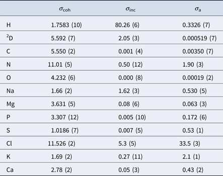
In aqueous solutions of proteins, the by far highest neutron scattering cross-section is the incoherent scattering cross-section of 1H, as reported in Table 2. Since proteins are largely composed of hydrogen, their main contribution to the neutron scattering function is incoherent, at least at scattering vectors q sufficiently far from correlation peaks. Moreover, given that deuterium (D) atoms have a much smaller cross-section than H-atoms, one can dissolve proteins in D2O rather than in H2O, thereby significantly reducing the signal of the solvent. Therefore, although the impact of the replacement of H2O with D2O on the protein dynamics should be considered (see section ‘From powder to solution: influence of solution conditions on protein dynamics’), neutron scattering is well-suited to access the self-dynamics of proteins in solution.
Coherent (σ coh), incoherent (σ inc) and absorption (σ a) neutron cross-sections in barns of the elements comprising proteins and common salts in biological environments (Sears, Reference Sears1992)
As an example, considering a colloidal particle undergoing free translational Fickian diffusion, the van Hove self-correlation function G s(r, t) is given by the probability density function (Vineyard, Reference Vineyard1958):
 $$G_{\rm s}\lpar {{\bf r}, \!t} \rpar = \displaystyle{1 \over {{(4\pi \,D^{\lpar {\rm s} \rpar }\,t)}^{d/2}}}\exp \left( {-\displaystyle{{{({\bf r}-{\bf r}_0)}^2} \over {4\,D^{{\rm (s)}}t}}} \right),$$
with the self-diffusion coefficient D (s), and the dimension d. The double Fourier transform of G s(r, t) yields a Lorentzian function
 $$S(q,\omega ) = \displaystyle{1 \over \pi} \; \displaystyle{\gamma \over {\gamma ^2 + \omega ^2}}\,,$$
with half width at half maximum (HWHM)  $\gamma = D^{(s)}q^2 $. For proteins, typical time-scales for short-time diffusion are on the order of nanoseconds, which correspond to γ ~ 1 μeV at q ~ 1 Å−1. These energy transfer and scattering vector ranges are directly accessible by quasi-elastic neutron backscattering (NBS).
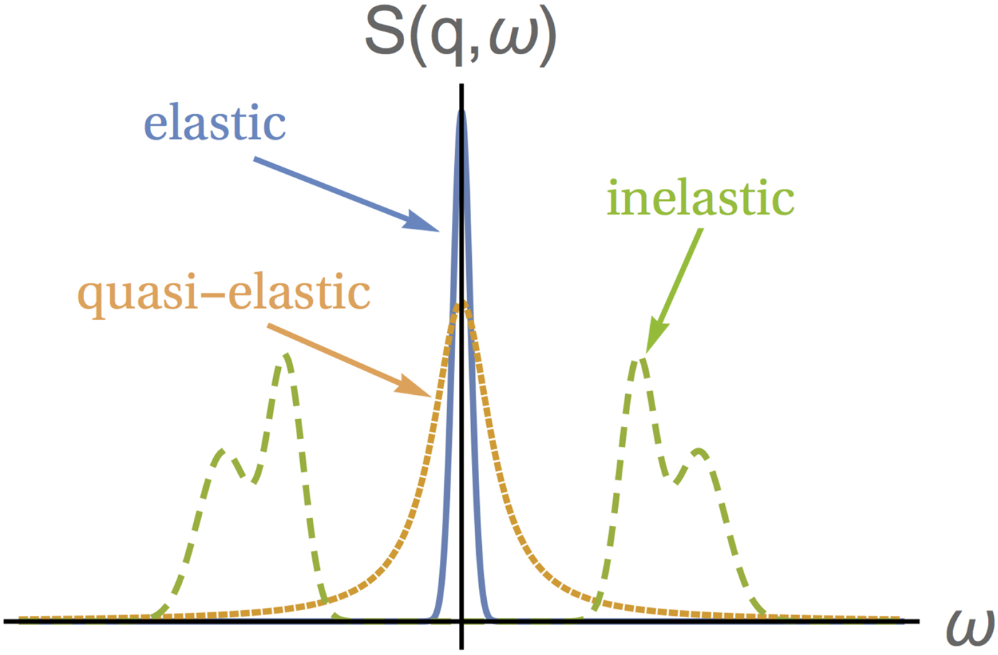
Depending on the energy transfer spectrum, three types of scattering can be identified, as shown in Fig. 5: (i) elastic scattering occurs when the spectrum is, ideally, a delta function centered at  $\hbar \! \omega = 0$, implying no dynamics in the sample. Note that, in practice, the delta function is always convoluted with a resolution function specific for every instrument, which in combination with a given statistics also limits the longest observable correlation time (cf. section ‘Experimental techniques’). (ii) QENS corresponds to a broadening of the elastic spectrum due to the movement of the scattering centers in the sample. Hence, the spectrum is broader than in the elastic case but, importantly, it still features a peak centered at zero energy transfer, hence the term quasi-elastic. For instance, in the case of diffusion, quasi-elastic scattering resulting in a scattering function with a Lorentzian profile centered at $\hbar\!\omega = 0$ is expected, as seen in Eq. (21). Typical broadenings γ due to protein diffusion in solution are on the order of eV for 0.2 Å−1 ${\rm \lesssim} \;q\;{\rm \lesssim} 2\,$Å−1. (iii) If the spectrum presents peaks centered at $\hbar\!\omega \ne 0$, the scattering is inelastic. Inelastic scattering is due to e.g. vibrational modes, typically at energies of a few millielectronvolts.
Sketch of the scattering function of elastic, quasi-elastic and inelastic neutron scattering near room temperature, in the absence of so-called detailed-balance effects. Elastic scattering gives a very sharp peak centered at ω = 0. QENS yields a broader peak centered at ω = 0, while the scattering function of inelastic scattering is characterized by peaks centered at ω ≠ 0. Figure rendered using Mathematica (Wolfram Research, Inc.).
In the case of elastic scattering, the magnitude of the wavevectors of the incoming (ki) and outgoing (kf) neutron is the same, and
 $$q\equiv \vert {\bf q} \vert = \displaystyle{{4\pi} \over \lambda} \sin \left( {\displaystyle{{2\theta} \over 2}} \right)\,,$$
where 2θ is the angle between ki and kf (see Fig. 4). Equation (22) also holds within the experimental accuracy for QENS.
The well-established theoretical framework for neutron scattering presented above involves some classical physics approximations. In a recent work by Kneller (Reference Kneller2018), incoherent neutron scattering is interpreted in terms of quantum mechanical transition rather than on classical displacement probabilities. The approach results in expressions for the scattering functions enabling an energy landscape-oriented analysis of neutron scattering spectra as well as a physical interpretation of Van Hove's space–time correlation functions in the quantum regime. With this formalism being so recent, so far we are not aware of published applications in the context of biophysical research. Therefore, although it may be employed in future studies, it will not be further discussed here.
Relevance of QENS for protein dynamics
Neutron spectroscopy is a remarkable technique to study protein dynamics for a number of reasons. Cold neutrons interact only weakly with matter, which allows the measurement of fragile biological samples such as proteins with negligible radiation damage. Also, generally, high protein concentrations typical of cell environments and turbid solutions can be easily measured, as opposed to optical techniques. Moreover, the neutrons are scattered particularly well by the hydrogen atoms compared with the other elements in proteins (Table 2). Such a scattering is mainly incoherent, meaning ultimately that neutron spectroscopy can provide information on the self-correlations of the rather homogeneously distributed hydrogen atoms, which allows for a label-free measurement of the average protein dynamics. Furthermore, the coherent scattering can be exploited to provide information on collective motions e.g. of protein domains.
Since the hydrogen atoms in H2O scatter neutrons just as well as those in proteins, a common workaround is to use D2O as a solvent, due to the much lower scattering cross-section of deuterium atoms compared with hydrogen atoms (cf. Table 2). The same principle can be used within the macromolecules: proteins can be synthesized in such a way that the hydrogen atoms in specific domains and sub-domains are exchanged with deuterium atoms (D-labeling), thus information on selected parts can be obtained.
Neutron instruments used for the spectroscopy of protein samples generally operate with an incident neutron energy on the order of a few millielectronvolts. This energy, corresponding to the so-called cold or thermal neutrons, is commensurate with the diffusive motions as well as the low-energy vibrational excitations of the proteins at the molecular level. Moreover, these neutron energies permit to access scattering vectors that are in a biologically interesting range from several hundred nanometers down to around 0.1 nm. A trivial advantage of cold or thermal neutron beams is the absence of radiation damage in biological samples, since the neutron energy is too low for ionization or the destruction of chemical bonds. Furthermore, neutron spectroscopy carries the additional advantage of directly accessing the atom motions, and not being affected by selection rules. These features make neutron spectroscopy a unique tool to study geometrical and dynamical features of protein dynamics at different levels, while of course other techniques provide highly complementary information (cf. section ‘Overview: techniques addressing protein dynamics’).
Experimental techniques
Neutron beams for condensed matter research emerge from nuclear fission or spallation processes. Depending on the employed process of neutron production, neutron sources produce neutron beams that are either continuous in time or display a pulse pattern. As the first step after neutron production, the initial neutron energy on the order of 1–10 MeV has to be reduced to the meV energy range using cold or thermal neutron moderators at fixed temperatures. The minimum path length of a few centimeters necessary to moderate neutron energies ultimately defines the source size. After moderation, neutron guides deliver the neutrons to the instruments. Although focus optics reduce the initial beam size at most modern neutron spectrometers, the source size sets already the size scale for the beam size at the sample, since the cost of the increasing divergence of a focused beam mostly sets the lower limit of the characteristic cross-section of a neutron beam at the sample to ~2.2 cm2.
Neutron spectrometers are subject to continuous progress in neutron optics to make optimal use of the available source flux from current and future neutron sources. Although neutron spectrometers can be generally classified based on their type of neutron detection, the given beam characteristics at different sources require specific adaptations and optimizations, rendering each instrument a unique neutron spectrometer with characteristics complementary to others.
In most cases, protein samples investigated by neutron spectroscopy are not in a crystalline but in a liquid solution, gel, glass or (hydrated) powder state. For this reason, the prevailing types of neutron spectrometers employed to study the dynamics of proteins comprise time-of-flight (TOF) and backscattering spectrometers as well as spin-echo spectrometers. These types of spectrometers will be reviewed in this section. Another class of neutron spectrometers, the triple-axis spectrometers, is less frequently used for the protein samples. Triple-axis spectrometers define both ki and kf by Bragg reflections from single crystals. Employing different setups, triple-axis spectroscopy covers a q-range from 10−3 up to almost 102 Å−1 and a  $\hbar\!\omega $-range from ~10 μeV to ~100 meV, with energy resolutions from some μeV to several millielectronvolts (Shirane et al., Reference Shirane, Shapiro and Tranquada2002). Their disadvantage for the study of powder samples is that they generally access only one pair (ki, kf) at once. However, a future advantage of triple-axis spectrometers may be the possibility to implement polarization analysis more easily than on other types of spectrometers. Moreover, triple-axis spectrometers can be combined with certain types of spin-echo techniques (Pynn, Reference Pynn1978) that are beyond the scope of this review.
Since energy-dispersive detectors do not exist for cold or thermal neutrons, a variety of different techniques has been developed to determine the energy of a scattered neutron. The TOF, backscattering and spin-echo techniques are named after three different ways to measure the energy of a cold or thermal neutron, namely by measuring its speed via its flight time over a known distance, by measuring its wavelength via a Bragg reflection, or by inferring the flight time from the number of its spin precessions while traveling through a magnetic field of known dimensions, respectively. The design of these spectrometers is mainly given by the specification of a desired resolution or coherence volume in reciprocal space and time and its optimal propagation through the primary (before the sample) and secondary (behind the sample) neutron optics. Optimal in this respect generally implies that the primary and secondary resolutions are identical, i.e. contribute equally to the Gaussian error propagation.
Time-of-flight (TOF) spectroscopy
TOF spectrometers are the most common instruments for QENS. The basic idea is to measure changes in energy by the TOF of the neutron. For this purpose, the sample is illuminated by a pulsed monochromatic beam. Subsequent to a short illuminating pulse, the sample remains ‘dark’ while the detectors count, as a function of time, the neutrons having been scattered by the sample. Each detected neutron is sorted in an acquisition channel according to its arrival time. With the known fixed flight path of typically 2–3 m from the sample to the detector, the detected neutron velocity and thus energy E = 1/2 mv2 can be easily obtained. The ‘classical’ TOF spectrometer such as TOFTOF at the MLZ (Unruh et al., Reference Unruh, Neuhaus and Petry2007) is a disk chopper spectrometer where a series of rotating chopper disks with narrow slits on their circumference is mounted with their center axis parallel to the neutron beam. These choppers provide the monochromatic incident beam. The resulting time series of brief openings allows neutrons to pass in an elaborate time pattern through the subsequent disks that are typically mounted with a distance of a few meters relative to each other. Both the individual disk speeds and their relative phases can be freely adjusted up to technically limited maximum speeds. On a continuous neutron source, in this way the incident wavelength and frame spacing can be freely tuned, which also varies the energy resolution greatly. A typical elastic energy resolution with cold neutrons at 5 Å is 90 μeV full width at half maximum (FWHM). The accessible range in the neutron energy transfer is limited by the initial neutron energy on the neutron energy loss side of the spectrum. The spectral range is in principle unlimited on the neutron energy gain side. However, the energy resolution drops with increasing energy. The large detectable range in energy transfers on TOF spectrometers allows to measure, besides QENS, also the low-energy inelastic scattering from molecular vibrations from some 100 μeV up to on the order of 1 eV. TOF instruments are therefore also particularly well-suited for phonon spectroscopy. Typical cold neutron TOF spectrometers are, hence, also THz spectrometers. These neutron THz spectra can be compared e.g. to photon and dielectric THz spectra.
Variants of TOF spectrometers are, among others, the so-called Fermi-chopper spectrometers and hybrid spectrometers that use the so-called mosaic crystals as monochromators. The latter can employ a series of several such crystals to become the so-called time-focusing TOF spectrometers such as FOCUS at SINQ (Janßen et al., Reference Janßen, Mesot, Holitzner, Furrer and Hempelmann1997).
Novel designs at pulsed neutron sources with a low pulse frequency (so-called long-pulse target stations) allow for TOF spectrometers such as LET at ISIS (Bewley et al., Reference Bewley, Taylor and Bennington2011) that can record QENS spectra at several incident energies in a quasi-instantaneous mode (at the expense of the inelastic information). A typical TOF spectrometer layout is depicted in Fig. 6. Several typical TOF spectrometers at neutron facilities worldwide are summarized in Table 3.
Simplified schematic representation of a TOF spectrometer at a reactor neutron source: a continuous ‘white’ neutron beam enters from the far left, passing a series of chopper disks (marked by the numbers 1–3). The total of six choppers in the chosen example setup are, from left, a pair of counter-rotating pulse choppers (1) chopping the continuous neutron beam into short pulses, the so-called contamination order and frame overlap choppers (2), and the pair of counter-rotating monochromator choppers (3). Each chopper carries a slit with an opening on its circumference that has an open area equal to the neutron guide cross-section area. The remainder of the chopper disk area absorbs neutrons. The counter-rotating chopper pairs serve to minimize the opening and closing times, thus enhancing the energy resolution. The sample (small red cylinder, 4) is located close to the last downstream chopper (3), typically tens of meters away from the pulse choppers. The detectors (long cyan cylindrical tubes, 5) cover a large solid angle at a neutron flight distance of several meters from the sample to simultaneously detect neutrons at multiple scattering angles. Figure rendered using Mathematica (Wolfram Research, Inc.).
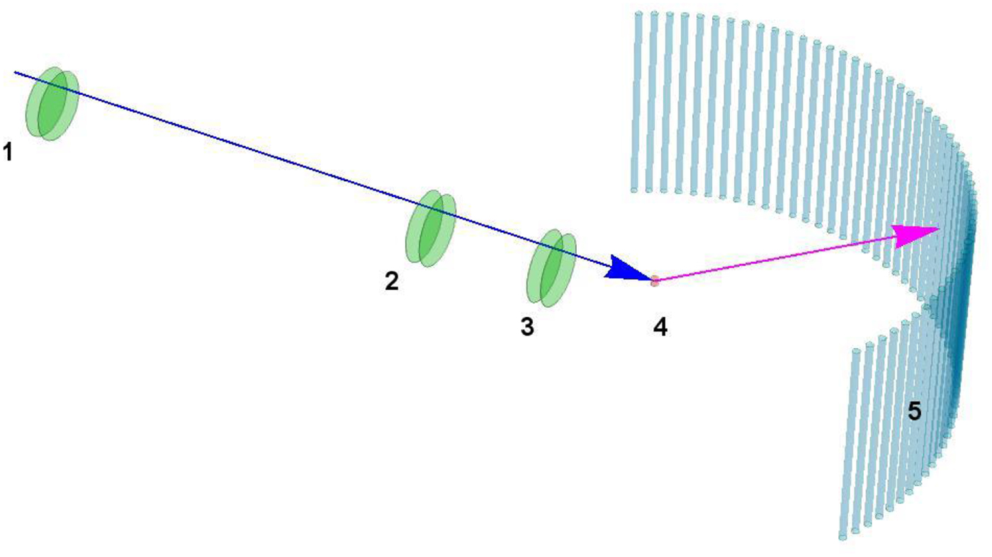
Neutron spectrometers with characteristics suitable for protein dynamics

We categorize the instruments along their fundamental measurement principles: NSE, neutron spin echo spectroscopy; NBS, neutron backscattering spectroscopy; TOF-NBS, combined time-of-flight backscattering spectroscopy; SA-TOF, small angle time-of-flight spectroscopy; TOF, neutron time-of-flight spectroscopy. Due to limited space, not all instruments and all configurations could be listed. We apologize for any omissions, which are not intentional.
a Sources: Reactor: ANSTO, Australian Nuclear Science and Technology Organisation, Lucas Heights, Australia; FLNP, Frank Laboratory of Neutron Physics, Dubna, Russia; ILL, Institut Laue-Langevin, Grenoble, France; LLB, Laboratoire Léon Brillouin, Saclay, France; MLZ, Heinz Maier-Leibnitz Zentrum, Garching, Germany; NCNR, NIST Center for Neutron Research, Gaithersburg, MD, USA. Spallation: ESS, European Spallation Source, Lund, Sweden (under construction); ISIS, STFC Rutherford Appleton Laboratory, UK; J-PARC, Japan Proton Accelerator Complex, Tokai, Ibaraki, Japan; SINQ, Swiss Spallation Neutron Source, Paul-Scherrer-Insitut, Villingen, Switzerland; SNS, Spallation Neutron Source, Oak Ridge National Laboratory, TN, USA; JCNS, Jülich Center for Neutron Sciences, Jülich, Germany.
Neutron backscattering (NBS) spectroscopy
The purpose of a backscattering spectrometer is to achieve a high energy resolution in the range of 0.5 μeV ⩽ Δω ⩽ 10 μeV FWHM, corresponding to an access to nanosecond relaxation timescales. To this end, NBS employs Bragg reflections at nearly or exactly vertical incidence on single crystals to achieve the highest possible definition of the neutron energy as becomes clear by the first derivative of Bragg's law,
 $$\displaystyle{{\delta E} \over E} = \displaystyle{{\delta d_{hkl}} \over {d_{hkl}}} + {\rm cot}({\rm \Theta} )\,\delta {\rm \Theta}, $$
where d hkl denotes the crystal lattice interplanar distance. Hence, the highest energy resolution is obtained for Θ = 90°, around which the contribution of the beam divergence is minimum.
Backscattering spectrometers at continuous cold neutron sources generally use exact backscattering both to define the incident neutron energy and the analyzed neutron energy. They achieve energy resolutions of ~0.75–0.9 µeV using bent Si crystals, depending on the crystal thickness. This resolution can be further enhanced by using flat Si crystals (at the expense of flux and a deviation from a Gaussian resolution line shape) or possibly further in the future by using GaAs crystals as an option on IN16B. Moreover, IN16B allows for the use of Si311 crystals. IN16B (Frick et al., Reference Frick, Mamontov, Eijck and Seydel2010), HFBS (Meyer et al., Reference Meyer, Dimeo, Gehring and Neumann2003) and SPHERES (Wuttke et al., Reference Wuttke, Budwig, Drochner, Kämmerling, Kayser, Kleines, Ossovyi, Pardo, Prager, Richter, Schneider, Schneider and Staringer2012) in addition possess a so-called phase-space transformer (PST) (Hennig et al., Reference Hennig, Frick and Seydel2011) for a flux enhancement at the sample. IN13 (Natali et al., Reference Natali, Peters, Russo, Barbieri, Chiapponi, Cupane, Deriu, Bari, Farhi, Gerelli, Mariani, Paciaroni, Rivasseau, Schiro and Sonvico2008) at the ILL employs CaF-analyzers, displaying a slight deviation from backscattering at the monochromator, and uses neutrons at higher energies in the thermal range.
Backscattering spectroscopy accesses the quasi-elastic spectrum of a sample typically in a range from ~1 to 100 μeV. A schematic representation of a standard backscattering spectrometer is shown in Fig. 7, and its principle is further illustrated in Fig. 8. NBS spectrometers are generally designed as so-called inverted geometry spectrometers, i.e. the incident energy is varied to record a spectrum, while the analyzed energy is kept fixed. This requirement results from the large analyzer surfaces usually employed (cf. Fig. 7). Depending on whether a pulsed or a continuous neutron source is employed, the incident energy is either scanned by detuning the effective monochromator lattice spacing relative to the analyzer lattice spacing, or by letting a very short source pulse spread in energy over a long distance on the order of 100 m (TOF method). For the former method, the effective monochromator lattice spacing can be detuned either by varying the crystal temperature (as employed on IN13; Natali et al., Reference Natali, Peters, Russo, Barbieri, Chiapponi, Cupane, Deriu, Bari, Farhi, Gerelli, Mariani, Paciaroni, Rivasseau, Schiro and Sonvico2008), or by mechanically moving the monochromator along its optical axis in order to achieve an apparent Doppler shift of the incident energy (effectively being explained by a Bragg reflection in a moving reference frame).
Schematic representation of the backscattering spectrometer IN16B at the ILL. A polychromatic (‘pink’) neutron beam (dashed line) illuminates the so-called PST (disk in the figure marked by ‘1’), which reflects the beam toward the backscattering monochromator (far bottom left, 2). This single crystal sends the monochromatic neutrons back toward the PST (1), which lets pass this neutron bunch via an open segment in the disk toward the sample (illustrated by the small cylinder, 3). The scattered neutrons are analyzed by the large crystals mounted on the surface of a sphere with a radius of 2 m, and the sample at its center (right part of the image, 4). The analyzed neutrons are detected by the detector tubes mounted right behind the sample (5). Figure rendered using Mathematica (Wolfram Research, Inc.), adapted from Hennig (Reference Hennig2011).
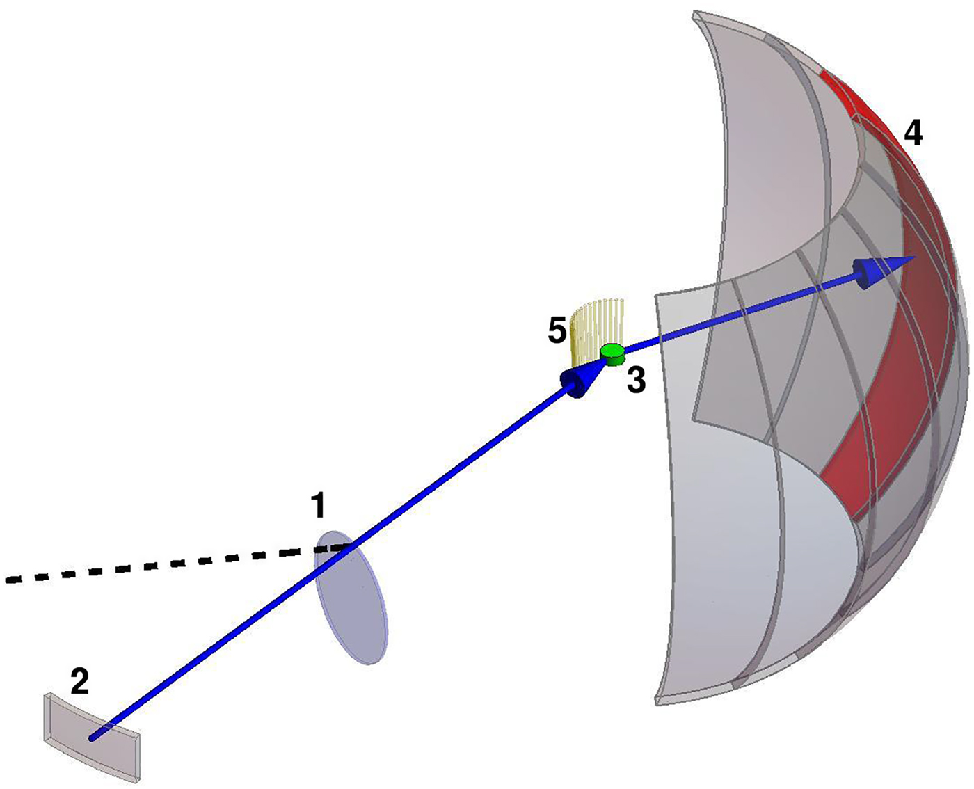
Schematic of the principle of a backscattering spectrometer. In the example, a neutron with energy E 0 + δE is delivered to the sample, where E 0 is the energy in backscattering from the analyzer crystals. After scattering by the sample, if the energy transfer equals − δE the neutron is reflected by the analyzers and detected; if the energy transfer differs from − δE the neutron is not reflected and is usually absorbed by absorbing material placed behind the analyzers. The thickness of the sample is chosen such that the probability for a neutron to be scattered once is  $\sim 10{\rm \%} $ and that of being scattered twice is hence $\sim \!1{\rm \%} $. The distance from the sample to the analyzers is typically 2 m, while the distance from the sample to the detectors amounts to <0.2m. Figure rendered using Mathematica (Wolfram Research, Inc.).
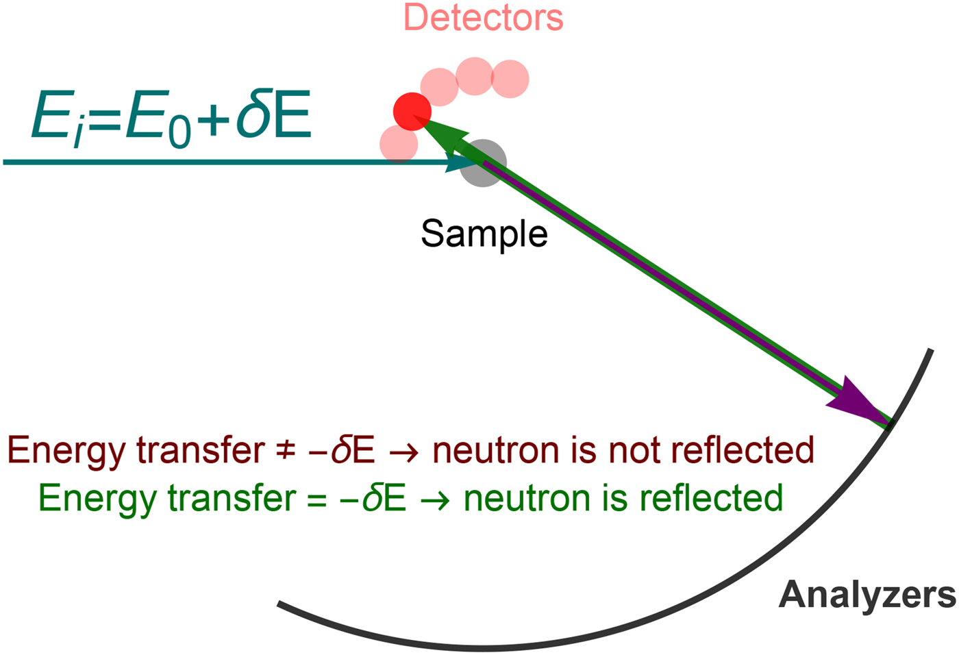
In the case of the latter method, the combined TOF backscattering spectrometers (TOF-NBS such as BASIS; Mamontov and Herwig, Reference Mamontov and Herwig2011), which use the flight time to define the incident neutron energy and backscattering from single crystals in the secondary spectrometer, in most cases allow for a slight deviation from exact backscattering. This deviation is matched to the incident resolution and results in an overall broader resolution function compared with continuous-source backscattering spectrometers. In most cases, these TOF-NBS instruments are located at pulsed neutron sources and are optimized for the time structure of these sources.
The rather involved backscattering setup requires that the neutrons scattered by the sample and having been backscattered by the analyzers travel backward in their original path toward the detectors (Fig. 8). The discrimination of outgoing and returning neutrons is therefore achieved by their flight time, and backscattering spectrometers at continuous sources use pulse choppers with an ~50% duty cycle for this purpose, while pulsed neutron sources are ‘dark’ for most of the time anyway. Note that the scattering probability by the sample is in general chosen to be <10% such that for the same neutron to be scattered a second time upon return is negligible.
Some NBS spectrometers worldwide are listed in Table 3.
Neutron spin-echo (NSE) spectroscopy
Following the TOF technique and the single-crystal technique, NSE spectroscopy (Mezei, Reference Mezei1972) provides the third option for the measurement of a neutron energy, or, more accurately, the change of the energy of a neutron. A fundamental idea of NSE is that, similar to interferometry, small changes in the energy of a neutron can be measured without knowing the absolute energy of this neutron precisely. The basic idea of a NSE spectrometer is to infer on the difference in the total number of spin precessions of a neutron in two equal magnetic fields, one of the fields being located upstream and the other downstream from the sample. This difference in the spin precessions is obtained indirectly by measuring the change in the polarization of a given neutron in the scattering process. If the polarization of a neutron changes differently in the second, identical magnetic field, it follows that this given neutron must have undergone a different number of spin precessions in that second field. Since with this concept, in a first approximation, only the change in the number of spin precessions is relevant to determine the change in the energy of a neutron, a spin echo spectrometer does not require a very good monochromaticity of the incident radiation. Importantly therefore, a spin echo spectrometer does not measure absolute energies, but accesses a correlation function in time associating the polarizations of the incident and scattered neutrons. From this information, the intermediate scattering function I(q,t) of the sample is obtained (Mezei et al., Reference Mezei, Pappas and Gutberlet2002) (cf. section ‘Modeling and analysis’). The monochromaticity of the incident beam is in this context still important for the definition of the scattering vector. Typically, a monochromaticity of Δλ/λ ≈ 0.08 is employed. This incident Δλ/λ is two orders of magnitude larger than on a typical backscattering spectrometer, implying largely increase neutron flux. The technical implementation of spin echo spectrometers is quite complex, and a large variety of designs can be found. Reviewing these would be beyond the scope of this paper. The reader is referred to the book by Mezei et al. (Reference Mezei, Pappas and Gutberlet2002). Novel instruments (Fouquet et al., Reference Fouquet, Ehlers, Farago, Pappas and Mezei2007; Farago et al., Reference Farago, Falus, Hoffmann, Gradzielski, Thomas and Gomez2015) benefit particularly from progress both in the strength and in the accurate geometry of magnetic fields.
In practical terms, the intermediate scattering function obtained from an NSE experiment is analogous to the scattering function obtained in a photon correlation spectroscopy experiment (i.e. DLS or XPCS). In NSE, only a small number of polarizations needs to be measured per data point in I(q,t). This requirement differs strongly from the necessary photon statistics that has to be obtained in a photon correlation spectroscopy experiment (be it using visible or X-ray photons) in order to build the photon intensity autocorrelation function for one point in I(q,t). NSE can therefore provide conceptually similar results compared with photon correlation spectroscopy despite the significantly weaker flux at neutron sources compared with visible or X-ray laser sources. Also, due the polarization analysis inherent to NSE, it distinguishes coherent and incoherent scattering. A standard NSE experiment records the coherent scattering analogous to a photon correlation spectroscopy experiment. Incoherent scattering by the sample in this case is rather a nuisance, but NSE can also be used to specifically explore incoherent scattering.
NSE can access very high relaxation-times (up to microseconds) and, thus, very slow motions, but requires long incident wavelengths implying relatively small scattering vectors. Nevertheless, the accessed scattering vectors are significantly larger than those obtained in DLS experiments, and NSE is obviously not limited to transparent samples. NSE does encounter difficulties when applied to magnetic samples that manipulate the neutron spin in the scattering process, but this issue is of little relevance for protein samples. Example NSE spectrometers worldwide are listed in Table 3, and a typical NSE layout is depicted in Fig. 9.
Simplified schematic representation of a spin echo spectrometer. A neutron beam with a typical wavelength spread of  $\Delta \lambda /\lambda \approx 8{\rm \%} $ impinges from the left and first passes a polarizer and π/2- (i.e. 90°-)spin-flipper (marked by ‘1’). In a classical picture, this device ‘flips’ the neutron spin axis to be perpendicular to their flight axis. The beam subsequently enters a first, homogeneous magnetic field, illustrated by the schematic cylindrical coil (2). The neutron spins precess in this first magnetic field, as indicated by the arrows perpendicular to the optical axis and illuminate the sample (3) illustrated by the square box. The scattered neutrons pass _a_ π-spin flipper behind the sample (4) to invert their spin and enter a second, equivalent magnetic field indicated by the cylindrical coil on the right side of the figure (5), where they precess again and finally pass a π/2-flipper and polarization analyzer (6) and hit the detector (7). If the neutrons are elastically scattered by the sample, they will have the same polarization in (6) as they have had in (1) due to this symmetric setup. In contrast, any change in their velocity by the scattering in the sample will change their initial polarization. The scattering angle 2Θ is adjusted by rotating the arm (4–7) around the sample (3). Figure rendered using Mathematica (Wolfram Research, Inc.), adapted from Hennig (Reference Hennig2011).

Modeling and analysis
The full hierarchy of motions ranging from translational and rotational diffusion of the entire molecule over large-scale domain motions down to localized dynamics of backbone and side-chains (see section ‘Protein dynamics on hierarchical time- and length-scales’) is represented in the quasielastic spectrum S(q,ω) in a convoluted way. While qualitative dynamical changes can be already observed from the spectra alone, extracting more detailed and quantitative information on the underlying dynamics requires modeling and data fitting, and potentially comparison with simulation (Vural et al., Reference Vural, Hu, Lindner, Jain, Miao, Cheng, Liu, Hong and Smith2017). In the following sections, we outline the basic modeling approaches to address the different hierarchical levels of protein dynamics.
Diffusion of the entire protein
Translations and rotations of the entire protein molecule are in a good approximation independent of the internal dynamics. They do, however, depend on the protein structure and size as well as the concentration of protein and other crowder molecules in solutions. Here, we will first outline two modeling approaches for the combined effect of translational and rotational diffusion. Second, we briefly revisit how interprotein interactions can be incorporated based on colloid theory.
Combination of translational and rotational diffusion
The translational diffusion of the center of mass of the protein results in a Lorentzian scattering function (cf. Eqs. (20) and (21)). However, also the rotation of the protein is a diffusive process, and causes an additional broadening of the quasi-elastic spectrum, which is practically indistinguishable from an effectively enhanced translational diffusion (Pérez et al., Reference Pérez, Zanotti and Durand1999; Roosen-Runge et al., Reference Roosen-Runge, Hennig, Zhang, Jacobs, Sztucki, Schober, Seydel and Schreiber2011), and modeling is key to extract more detailed information.
One approach to model these global contributions to protein dynamics is to calculate the diffusion tensor based on protein structures using software packages such as HYDROPRO (de la Torre et al., Reference de la Torre, Huertas and Carrasco2000). This approach accounts for the full anisotropy of the shape and diffusion, but depends on an available protein structure, which furthermore is assumed to be rigid. From the diffusion tensor D, the apparent collective diffusion coefficient  $D_{{\rm app}}^{\lpar {\rm c} \rpar } (q)$ is given by (Biehl et al., Reference Biehl, Monkenbusch and Richter2011; Stingaciu et al., Reference Stingaciu, Ivanova, Ohl, Biehl and Richter2016)
 $$ D_{{\rm app}}^{\lpar {\rm c} \rpar } \lpar q \rpar = \displaystyle{1 \over {P\lpar q \rpar }}\left\langle {\mathop \sum \limits_{\alpha, \beta} b_\alpha^{{\rm coh}} b_\beta^{{\rm coh}} {\rm e}^{i{\bf q}\cdot \lpar {{\bf r}_\alpha -{\bf r}_\beta} \rpar }} \right.\left. {\left( {\matrix{ {\hat{{\bf q}}} \cr {{\hat{\bf q} \times} {\bf r}_\alpha} \cr}} \right){\bf D}\left( {\matrix{ {\hat{{\bf q}}} \cr {{\hat{\bf q} \times} {\bf r}_\beta} \cr}} \right)} \right\rangle $$
where  $P\lpar q \rpar = \left\langle {\sum\nolimits_{\alpha, \beta} {b_\alpha^{{\rm coh}} b_\beta^{{\rm coh}} {\rm e}^{i{\bf q}\cdot \lpar {{\bf r}_\alpha -{\bf r}_\beta} \rpar }}} \right\rangle $ is the form factor of the particle and b i and r i denote the scattering length and the coordinate of the individual atoms. The related autocorrelation functions are represented as $I\lpar {q,t} \rpar = \exp {\rm \;} (-6D_{{\rm app}}^{\lpar {\rm c} \rpar } t)$. Note that a similar evaluation is in principle possible for the apparent self-diffusion coefficient by collapsing the double sum to a single sum with j = k.
A different coarse-grained (CG) approach has been to use effective (isotropic) translational and rotational diffusion coefficients D t and D r as an input, and study the resulting apparent diffusion coefficient. The explicit choice of the diffusion coefficients can be based on knowledge from other techniques, and allows to implicitly introduce effects of anisotropic shape (Harding, Reference Harding1995; Ferrer et al., Reference Ferrer, Duchowicz, Carrasco and Torre2001), permeability (Abade et al., Reference Abade, Cichocki, Ekiel-Jeyewska, Nägele and Wajnryb2010; Riest et al., Reference Riest, Eckert, Richtering and Nägele2015) and softness (Protopapas et al., Reference Protopapas, Andersen and Parlee1973; Senff and Richtering, Reference Senff and Richtering1999) into the effective hard sphere model (Jennings and Parslow, Reference Jennings and Parslow1988). The translational and rotational autocorrelations are represented as (Bee, Reference Bee1988; Pérez et al., Reference Pérez, Zanotti and Durand1999)
 $$I_{\rm t}\lpar {q, \!t} \rpar = \exp (-D_{\rm t}q^2t)$$
 $$I_{\rm r}\lpar {q,t} \rpar = \mathop \sum \limits_{l = 0}^\infty \exp {\rm } \! (-l\lpar {l + 1} \rpar D_{\rm r}t)B_{\rm l}\lpar q \rpar $$
where, depending on coherent or incoherent scattering,
 $$B_l^{{\rm coh}} \lpar q \rpar = \mathop \sum \limits_m \left \vert {\mathop \sum \limits_\alpha b_\alpha^{{\rm coh}} j_l\lpar {{\bf q}\cdot {\bf r}_\alpha} \rpar Y_{lm}\lpar {{\rm \Omega}_\alpha} \rpar } \right \vert ^2\;, $$
 $$B_l^{{\rm inc}} \lpar q \rpar = \int_0^\infty {{\rm d}r\,\rho \lpar r \rpar \lpar {2l + 1} \rpar j_l^2 \lpar {qr} \rpar } $$
with the orientation Ωα of the individual atoms, and the radial distribution function ρ(r) of incoherent scatterers, i.e. mainly hydrogen atoms. j l(x) denotes the spherical Bessel function of first kind, and Y lm(Ω) are spherical harmonic functions. We remark that the focus on hydrogen in the case of self-dynamics is valid since protons dominate the incoherent scattering. Generally, ρ(r) would be the radial distribution of incoherent scatterers.
Assuming a decoupling of translation and rotation, the total autocorrelation is multiplicative, I(q, t) = I t(q, t)I r(q, t). The resulting apparent diffusion coefficient D app can been calculated as the first cumulant via comparably expensive numerical integration (Pérez et al., Reference Pérez, Zanotti and Durand1999; Stadler et al., Reference Stadler, Digel, Artmann, Embs, Zaccai and Büldt2008) or the more efficient numerical solution of the analytical implicit expression (Roosen-Runge et al., Reference Roosen-Runge, Hennig, Zhang, Jacobs, Sztucki, Schober, Seydel and Schreiber2011; Grimaldo et al., Reference Grimaldo, Roosen-Runge, Jalarvo, Zamponi, Zanini, Hennig, Zhang, Schreiber and Seydel2015c)
 $$\mathop \sum \limits_{l = 0}^{l_{{\rm max}}} B_l(q)\displaystyle{{D_{\rm r}l\lpar {l + 1} \rpar + \lpar {D_{\rm t}-D_{{\rm app}}} \rpar q^2} \over {D_{\rm r}l\lpar {l + 1} \rpar + \lpar {D_{\rm t} + D_{{\rm app}}} \rpar q^2}} = 0$$
where l max has to be large enough to ensure convergence, depending on the evaluated q range. The apparent diffusion coefficient D app(q) starts off at low q with the value of D t. Around q ≈ 1/R p with the effective protein radius R p, D app(q) increases to a second plateau value at high q, which includes the contribution of translational and rotational diffusion (Grimaldo et al., Reference Grimaldo, Roosen-Runge, Jalarvo, Zamponi, Zanini, Hennig, Zhang, Schreiber and Seydel2015c).
Effects of crowding on diffusion
Interactions between proteins and crowding molecules inevitably alter the diffusion behavior. While self-diffusion is generally slowed down by crowding effects, repulsive interactions can increase collective diffusion on selected wavelengths (Nägele, Reference Nägele1996). Colloid theory has been found to provide a suitable reference for protein solutions, even in concentrated and strongly interacting suspensions and on different length and timescales (see e.g. Longeville et al. (Reference Longeville, Doster and Kali2003b); Doster and Longeville (Reference Doster and Longeville2007); Heinen et al. (Reference Heinen, Zanini, Roosen-Runge, Fedunova, Zhang, Hennig, Seydel, Schweins, Sztucki, Antalik, Schreiber and Nägele2012); Roosen-Runge et al. (Reference Roosen-Runge, Hennig, Zhang, Jacobs, Sztucki, Schober, Seydel and Schreiber2011) and references therein).
Importantly, colloid theory provides not only a qualitative understanding, but also quantitative predictions for self- and collective-diffusion coefficients. In particular, series expressions of the type
 $$D^{\lpar {\rm s} \rpar } = D_0\lpar {1 + a\varphi + \cdots} \rpar$$
have been derived for the dependence of translational and rotational self-diffusion on volume fraction φ for hard and charged spheres (Medina-Noyola, Reference Medina-Noyola1988; Tokuyama and Oppenheim, Reference Tokuyama and Oppenheim1994; Banchio and Nägele, Reference Banchio and Nägele2008).
For translational collective diffusion, the diffusion coefficient D(q) depends explicitly on the structure factor S(q) (Dhont, Reference Dhont1996; Nägele, Reference Nägele1996),
 $$D_{\rm t}^{\lpar {\rm c} \rpar } (q) = D_0\displaystyle{{H(q)} \over {S(q)}}$$
 The hydrodynamic function H(q) can be calculated based on information on the interparticle interaction (Beenakker and Mazur, Reference Beenakker and Mazur1984; Dhont, Reference Dhont1996; Nägele, Reference Nägele1996; Heinen et al., Reference Heinen, Zanini, Roosen-Runge, Fedunova, Zhang, Hennig, Seydel, Schweins, Sztucki, Antalik, Schreiber and Nägele2012), while the self-diffusion coefficient in the dilute limit, D 0, has to be provided by other experimental or modeling methods. In the high-q limit, in the absence of attractive interactions, S(q) → 1 and H(q) → D (s)/D 0, and hence  $D_{\rm t}^{\lpar {\rm c} \rpar } (q)\to D^{\lpar {\rm s} \rpar }$. Note that although the method has been developed for repulsive systems, it has also been applied successfully to mildly attractive systems (Riest and Nägele, Reference Riest and Nägele2015).
Large-scale and domain motions
Given the relevance of large-scale motions such as cleft opening for protein function, experimental access to these motions is of great importance. The determination of prevailing large-scale motions in proteins is, however, no trivial task, and depends in general on the availability of protein structures.
The most conventional approach for the analysis of experimental data of large-scale protein motions is a normal mode analysis aiming at the low-frequency Brownian modes (Hinsen, Reference Hinsen1998; Doruker et al., Reference Doruker, Atilgan and Bahar2000; Hinsen et al., Reference Hinsen, Petrescu, Dellerue, Bellissent-Funel and Kneller2000; Cui and Bahar, Reference Cui and Bahar2006), as implemented in open-source software packages such as the molecular modeling toolkit MMTK (Hinsen, Reference Hinsen2000) or ProDy (Bakan et al., Reference Bakan, Meireles and Bahar2011). The basic idea is to assume an elastic network of all atoms in the protein as a model of collective fluctuations around the equilibrium structure, which corresponds to the classical Ornstein–Uhlenbeck process. The force matrix  ${\bf K}_{\alpha \beta} = \left. {{\textstyle{{\partial^2E_{{\rm pot}}} \over {\partial R_\alpha \partial R_\beta}}}} \right\vert_{{\rm eq}}$ represents harmonic springs between atom α and β, usually varying with interatomic distance. In addition, atom-wise frictions γ α are introduced. The input parameters can be chosen either as semiempirical constants, or based on MD simulations (Hinsen et al., Reference Hinsen, Petrescu, Dellerue, Bellissent-Funel and Kneller2000).
The resulting autocorrelations are represented as (Kneller, Reference Kneller2000):
 $$I_{{\rm coh}}\lpar {q,\!t} \rpar = \left\langle {\mathop \sum \limits_{\alpha, \beta} b_\alpha^{{\rm coh}} b_\beta^{{\rm coh}} \exp \lpar {-i{\bf q}\cdot \lpar {{\bf R}_\alpha^{{\rm eq}} -{\bf R}_\beta^{{\rm eq}}} \rpar } \rpar f_{\alpha \beta} \lpar {{\bf q},\!t} \rpar } \right\rangle $$
 $$I_{{\rm inc}}\lpar {q,\!t} \rpar = \left\langle {\mathop \sum \limits_\alpha {\lpar {b_\alpha^{{\rm inc}}} \rpar }^2f_{\alpha \alpha} \lpar {{\bf q}, \!t} \rpar } \right\rangle $$
where  $R_\alpha ^{{\rm eq}} $ are the equilibrium positions of the atom α, and b α denote the scattering length (see section ‘Quasi-elastic neutron scattering theory’). The dynamical form factors f αβ(q, t) can be rewritten in a static and a time-dependent part (Kneller, Reference Kneller2000; Stingaciu et al., Reference Stingaciu, Ivanova, Ohl, Biehl and Richter2016):
 $$f_{\alpha \beta} \lpar {{\bf q}, \! t} \rpar = f_{\alpha \beta} \lpar {{\bf q}, \!\infty} \rpar {\,f}^{\prime}_{\alpha \beta} \lpar {{\bf q}, \!t} \rpar $$
 The static part as well as the initial equilibrium expression only depend on the harmonic potential, and are calculated using the eigenvalues ω j and orthonormal eigenvectors  $\hat{{\bf u}}_j$ of the mass-weighted force matrix ${\bf K}_{\alpha \beta} ^{\lpar m \rpar } = {\bf K}_{\alpha \beta} /\sqrt {m_\alpha m_\beta} $ as (Kneller, Reference Kneller2000)
 $$f_{\alpha \beta} \lpar {{\bf q}, \! \infty} \rpar = \exp \left( {-\displaystyle{{k_{\rm B}T} \over 2}\mathop \sum \limits_{\,j = 1}^{3N} \displaystyle{{{({\bf q}\cdot {\hat{{\bf u}}}_{\,j\alpha} )}^2 + {({\bf q}\cdot {\hat{{\bf u}}}_{\,j\beta} )}^2} \over {\omega_j^2}}} \right)$$
 $$f_{\alpha \beta} \lpar {{\bf q}, \!0} \rpar = \exp \left( {-\displaystyle{{k_{\rm B}T} \over 2}\mathop \sum \limits_{\,j = 1}^{3N} \displaystyle{{{({\bf q}\cdot {\hat{{\bf u}}}_{\,j\alpha} -{\bf q}\cdot {\hat{{\bf u}}}_{\,j\beta} )}^2} \over {\omega_j^2}}} \right)$$
with the displacement  $\hat{{\bf u}}_{j\alpha} $ of the atom α in the jth mode.
For the time-dependent part, the solution depends on the specific dynamics, see Kneller (Reference Kneller2000) for details. Assuming overdamped dynamics, the Brownian modes are given by the eigenvalues λ k and orthonormal eigenvectors  $\hat{{\bi v}}_k$ of the friction-weighted force matrix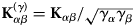 ${\bf K}_{\alpha \beta} ^{\lpar \gamma \rpar } = {\bf K}_{\alpha \beta} /\sqrt {\gamma _\alpha \gamma _\beta} $ and yield for the time-dependent part (Hinsen et al., Reference Hinsen, Petrescu, Dellerue, Bellissent-Funel and Kneller2000; Kneller, Reference Kneller2000)
 $${\,f}^{\prime}_{\alpha \beta} \lpar {q, \!t} \rpar = \exp \left( {\displaystyle{{k_{\rm B}T} \over {\sqrt {\gamma_\alpha \gamma_\beta}}}} \right.\left. {\mathop \sum \limits_{k = 1}^{3N} ({\bf q}\cdot {\hat{{\bf v}}}_{k\alpha} )\lpar {{\bf q}\cdot {\hat{{\bf v}}}_{k\beta}} \rpar \displaystyle{{{\rm exp}(-\lambda_kt)} \over {\lambda_k}}} \right)$$
with the displacement  $\hat{{\bf v}}_{k\alpha} $ of the atom α in the kth mode. A graphic visualization of a normal mode calculated for immunoglobulin G (IgG) is shown in Fig. 10.
Graphical representation of a normal mode of IgG (Harris et al., Reference Harris, Larson, Hasel and McPherson1997) obtained through the anisotropic network model for CG normal mode analysis (Eyal et al., Reference Eyal, Lum and Bahar2015).
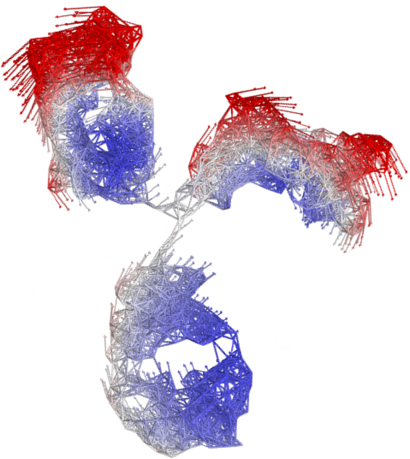
Considering the limited instrumental time window, not all relaxations will be resolved in the experiment. In particular, fast motions, i.e. higher order modes, will have relaxed already, and slower modes might be too slow to be resolved. Taking this into account, a simplified form suitable for data fitting can be derived when summarizing all modes in the accessible time window with an effective relaxation constant  $\bar{\lambda} $,
 $$I\lpar {q,t} \rpar /I\lpar {q,0} \rpar = I_{\rm t}\lpar {q,t} \rpar I_{\rm r}\lpar {q,t} \rpar \lpar {C\lpar q \rpar + A\lpar q \rpar \exp (-\bar{\lambda} t)} \rpar.$$
In principle, I(q,0) equals the form factor P(q). However, I(q,0) is usually determined from the experimental data, and thus effectively corrects for fast relaxations outside the experimental window as well as effects of incoherent scattering. After this correction, the slower motions that appear fixed during the experiment time are represented by the amplitude C(q) = 1 − A(q). Finally, A(q) for a set S of Brownian modes is given by (Biehl et al., Reference Biehl, Monkenbusch and Richter2011)
 $$\!\!\!\!A(q) = \mathop \sum \limits_{k\in S} a_k\mathop \sum \limits_{\alpha, \beta} b_\alpha b_\beta \exp\!\lpar {i{\bf q}\cdot \lpar {{\bf r}_\alpha -{\bf r}_\beta} \rpar } \rpar \lpar {\hat{{\bf q}}\cdot {\hat{{\bf v}}}_{k\alpha}} \rpar \lpar {\hat{{\bf q}}\cdot {\hat{{\bf v}}}_{k\beta}} \rpar $$
where the mode amplitudes a k depend on the friction constants and the temperature. A(q) as the q signature of internal motions has been successfully used to determine motional patterns occurring in proteins (Biehl et al., Reference Biehl, Hoffmann, Monkenbusch, Falus, Prévost, Merkel and Richter2008, Reference Biehl, Monkenbusch and Richter2011; Sill et al., Reference Sill, Biehl, Hoffmann, Radulescu, Appavou, Farago, Merkel and Richter2016).
It has to be mentioned that the standard normal mode analysis does not account for anharmonic potentials and effects of secondary structure as well as details in the friction within the protein and with water (Smolin et al., Reference Smolin, Biehl, Kneller, Richter and Smith2012). Nevertheless, results for the low-frequency normal modes are reasonably robust against changes of the representation from full-atomic detail to only backbone carbons or even small rigid blocks (Hinsen, Reference Hinsen1998; Tama et al., Reference Tama, Gadea, Marques and Sanejouand2000). Furthermore, the results can be compared with much more costly computer simulations aiming for the so-called essential dynamics or proteins, i.e. a smaller set of motions that describe larger protein motions with good accuracy (Amadei et al., Reference Amadei, Linssen and Berendsen1993). In particular, modes derived from singular value decomposition of simulated protein dynamics revealed similar signatures and cross-correlations as normal modes (Doruker et al., Reference Doruker, Atilgan and Bahar2000). Dynamical models can also be constructed and improved ad hoc, based on complementary techniques or intuition (Yang et al., Reference Yang, Song and Jernigan2007; Stingaciu et al., Reference Stingaciu, Ivanova, Ohl, Biehl and Richter2016).
Comparing the obtained signatures for large scale motions in proteins with experimentally accessible data e.g. from NSE spectroscopy allows to understand collective internal protein dynamics, and thus the underlying dynamical mechanisms of protein function.
Localized internal dynamics
Localized internal dynamics such as fluctuations of backbone and side-chains are intrinsic to the physicochemical properties of proteins. In the following, we present several conventional models for these fast motions on small length scales. As the basic model and analogously to the case of large-scale motions, two contributions are considered (Bee, Reference Bee1988):
 $$S_{{\rm int}}(q, \!\omega ) = A(q)\,\delta (\omega ) + (1-A(q))\,{\cal L} ({\rm \Gamma}, \!\omega )$$
The so-called elastic incoherent structure factor (EISF) A(q) (see section ‘Localized internal dynamics’) provides access to the confinement geometry of motions within the experimental time window. The effective relaxation constant Γ(q) (see section ‘Localized internal dynamics’) comprises all dynamical processes within the experimental time window, and thereby accesses the motional character of the underlying motions. Thus notably, neutron spectroscopy provides information on both geometrical and dynamical signatures of localized protein dynamics.
Confinement geometry of localized motions: elastic incoherent structure factor
The formal expression for the EISF is represented as (Kneller, Reference Kneller2000)
 $$A(q) = \mathop \sum \limits_\alpha b_\alpha ^2 \vert \exp \! \lpar {-i{\bf q}\cdot {\bf r}_\alpha} \rpar \vert ^{2.}$$
Given the dominant (incoherent) scattering contribution of hydrogen, the most common models focus on the motion of one representative atom in an effective confinement such as an impermeable sphere, a parabolic potential or a finite number of sites on a circle.
Diffusion in an isotropic confinement
The motion in an isotropic confinement has been modeled in two variants. First, considering free diffusion in an impermeable sphere with radius r, the EISF is represented as (Volino and Dianoux, Reference Volino and Dianoux1980; Press, Reference Press1981)
 $$A_{{\rm sph}}(q\,,R) = \left \vert {\displaystyle{{3j_1\lpar {qR} \rpar } \over {qR}}} \right \vert ^2$$
where j 1(x) = [sin(x) − x cos(x)]/x 2 denotes the first order spherical Bessel function of the first kind.
Second, assuming diffusion in a radial harmonic potential, a Gaussian density profile is obtained with a corresponding EISF of (Volino et al., Reference Volino, Perrin and Lyonnard2006)
 $$A_{\rm G}(q) = \exp \! \lpar {-q^2\langle{u^2} \rangle} \rpar \,.$$
 When the variance of the density profile is  $\langle u^2 \rangle \equals R^2 \hbox{/} 5$, both expressions are almost superimposed for $(q\,R)^2{\rm \lesssim} 5$ (Volino et al., Reference Volino, Perrin and Lyonnard2006). The radius R can be used to estimate the volume accessible to the hydrogen atoms in a protein, although there are no obvious reasons for this volume to be spherical. The radius obtained from the model is easily compared between different proteins and may be used as a rough indicator of the local structural flexibility and the ability of the protein to explore different conformations.
Jumps between three sites on a circle
In order to describe the geometrical confinement of the H-atoms in a methyl group, a model describing an atom jumping between three equivalent sites on the vertices of an equilateral triangle is commonly used. The expression for the EISF is given by (Press, Reference Press1981; Bee, Reference Bee1988; Bée, Reference Bée1992; Pérez et al., Reference Pérez, Zanotti and Durand1999):
 $$A_{3-j}\lpar {q,a} \rpar = \displaystyle{1 \over 3}[ {1 + 2\,j_0\lpar {qa} \rpar } ],$$
where j 0(x) = sin(x)/x is the zeroth order spherical Bessel function of the first kind and a denotes the jump-distance between two sites.
Combinations of models and immobile fraction
The EISF is usually described simply by a linear combination of these and similar models, whose amplitudes represent the fraction of hydrogens in the respective confinement. In most cases the total EISF is modeled as
 $$A(q) = p + (1-p)\,A_{{\rm model}}(q)\,,$$
where p denotes the number of atoms which remain immobile on the timescale accessible by the instrument, and A model(q) is one or a combination of the models presented above. It should be emphasized that these models provide a very simplified description of the complexity of the local confinement of atoms in a protein. Nevertheless, these simple models were successfully applied in previous studies to obtain valuable information on the confinement of the internal dynamics, and its dependence on several parameters. Further information on the topic and other models can be found e.g. in Bee (Reference Bee1988).
Dynamical signature of local motions
The internal self-dynamics as measured by QENS is usually modeled by one or more Lorentzian functions. As already seen in the ‘Quasi-elastic neutron scattering theory’ section (in particular Eq. (21)), simple Fickian diffusion of an unbound scatterer results in a HWHM of the quasi-elastic broadening Γ ∝ q 2.
In contrast, atoms in the protein are affected by a complex potential landscape with several minima, corresponding to preferred spatial configurations. Under such conditions, the functional form of Γ(q) changes significantly (Fig. 11). The resulting motion of atoms can be thought of as a sequence of effective jumps with rate 1/τ 0 between preferred configurations. Consequently, a behavior resembling free diffusion may be expected only on a length scale sufficiently large compared with the length of the jumps, i.e. at lower q. Furthermore, geometrical constraints due to e.g. steric interactions or chemical bond lengths limit the length scale on which dynamical processes occur. In the following, we present some of the models used for a description of the internal dynamics.
Comparison of the HWHM Γ as a function of q 2 for Fickian diffusion and jump-diffusion. For Fickian diffusion Γ = Dq 2: a straight line is obtained and the slope gives the diffusion coefficient D. For unrestricted jump-diffusion, the slope at low q gives the jump-diffusion coefficient D 1, and the asymptote at high q gives the inverse of the residence time τ 0. Figure rendered using Mathematica (Wolfram Research, Inc.).
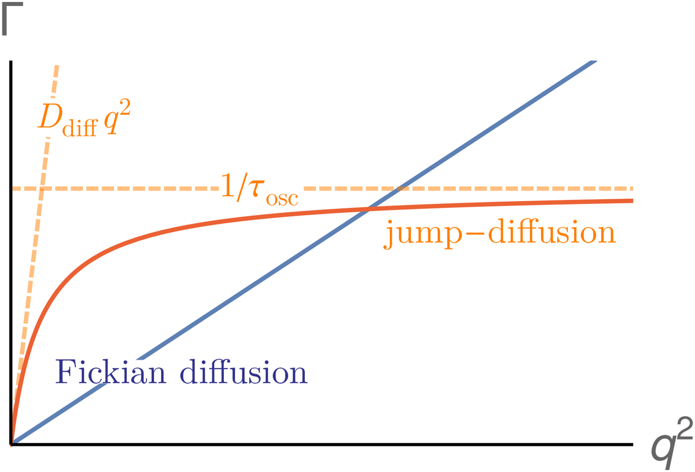
Jump-diffusion model
The jump-diffusion model by Singwi and Sjölander (Reference Singwi and Sjölander1960) describes a particle switching between an oscillation around an equilibrium position for a time τ osc, and a diffusive motion with diffusion coefficient D diff.
In order for the model to describe jump diffusion, the limiting case of a short diffusive period τ osc ≫ τ diff and very small oscillation amplitude is done, yielding a Lorentzian shape with HWHM (Singwi and Sjölander, Reference Singwi and Sjölander1960)
 $${\rm \Gamma} _{{\rm jump}}\lpar q \rpar = \displaystyle{{D_{{\rm diff}}q^2} \over {1 + D_{{\rm diff}}\tau _{{\rm osc}}\,q^2}}\;. $$
As shown in Fig. 11, a simple diffusive signature Γjump ≈ D diffq 2 is obtained for q → 0, whereas Γjump ≈ 1/τ 0 for q → ∞. This characteristic is typical for random jump-diffusion models, such as the one presented here or e.g. that by Hall and Ross (Reference Hall and Ross1981).
Diffusion in a Gaussian well and the overdamped Brownian oscillator
To describe a localized motion in a region of space with a soft boundary, Volino, Perrin, and Lyonnard (Volino et al., Reference Volino, Perrin and Lyonnard2006) have developed a model based on Gaussian statistics. Considering a particle moving isotropically and in three dimensions about the origin, under the assumption that the displacement u from the origin is a Gaussian random variable with variance  $\langle u^2 \rangle $, characterizing the region in which the particle is confined, and the normalized equilibrium density probability function is given by (Volino et al., Reference Volino, Perrin and Lyonnard2006):
 $$p(u) = \displaystyle{1 \over {{[ {2\pi \langle{u^2} \rangle} ] }^{1/2}}}\exp \left[ {-\displaystyle{{u^2} \over {2\langle{u^2}\rangle }}} \right]\,.$$
Then, the intermediate scattering function can be expressed as (Volino et al., Reference Volino, Perrin and Lyonnard2006):
 $$I\lpar {q, \! t} \rpar = \exp [ {-q^2\langle{u^2} \rangle \lpar {1-\rho \lpar t \rpar } \rpar } ] \,$$
with the correlation function ρ(t). In the case of a particle diffusing with a diffusion coefficient D eff, ρ(t) = exp[ −t·D eff/〈u 2〉] (Volino et al., Reference Volino, Perrin and Lyonnard2006; Stadler et al., Reference Stadler, Garvey, Embs, Koza, Unruh, Artmann and Zaccai2014a). Hence, for an overdamped Brownian oscillator, the intermediate scattering function becomes (Volino et al., Reference Volino, Perrin and Lyonnard2006; Stadler et al., Reference Stadler, Garvey, Embs, Koza, Unruh, Artmann and Zaccai2014a):
 $$I(q, \!t) = \exp [ {-q^2\langle u^2\rangle (1-\exp {\rm}\! [-t\,\cdot D_{{\rm eff}}/\langle u^2\rangle ])} ] \,,$$
and the scattering function is represented as (Volino et al., Reference Volino, Perrin and Lyonnard2006; Stadler et al., Reference Stadler, Garvey, Embs, Koza, Unruh, Artmann and Zaccai2014a):
 $$\eqalign{S\lpar {q, \! \omega} \rpar = &\exp [{-q^2\langle{u^2} \rangle} ] \cr & \times \left(\delta \lpar \omega \rpar + \mathop \sum \limits_{n = 1}^{\infty} \displaystyle{(q^2\langle u^2\rangle )^n \over n!} \right. \left. \displaystyle{1 \over 2\pi} \displaystyle{n\; D_{{\rm eff}\;} /\langle u^2\rangle \over n\; D_{\rm eff}\; /\langle u^2 \rangle + \omega^2} \right)}$$
D eff being an effective coefficient describing the diffusive motion of an atom within the protein, the model can be integrated with the jump-diffusion model if D eff(q) = D diff/(1 + D diffτ osc q 2) (Volino et al., Reference Volino, Perrin and Lyonnard2006). The scattering functions for the anisotropic case as well as for the two- and one-dimensional cases can be found in Volino et al. (Reference Volino, Perrin and Lyonnard2006).
Switching model between dynamical states
The jump-diffusion model presented in the previous subsection concerns a specific situation. However, the idea of a motion switching between dynamical states can be exploited in a more general way, providing analytical correlation functions for a larger class of dynamical switching processes (Roosen-Runge et al., Reference Roosen-Runge, Bicout and Barrat2016).
As one practical example, an atom switching between two diffusive states with relaxation constants Γ1(q) and Γ2(q) is considered. With switching rates 1/τ 1 and 1/τ 2 constant in time, one obtains a function with two Lorentzian profiles (Roosen-Runge et al., Reference Roosen-Runge, Bicout and Barrat2016)
 $$S_{{\rm sw}}(q, \!\omega ) = \alpha (q)\,{\cal L} (\lambda _1(q), \! \omega ) + (1-\alpha (q))\,{\cal L} (\lambda _2(q), \!\omega )$$
with HWHM λ 1 and λ 2, respectively, and
 $$\alpha = \tau_1\Gamma_2 + \tau_2\Gamma_1 + (\tau_1+\tau_2)(\tau_1^{-1} +\tau_1^{-1} - \lambda_1)$$
 $$\lambda _{1,2} = \displaystyle{{{\rm \Gamma} _1 + {\rm \Gamma} _2 + \tau _1^{-1} + \tau _2^{-1} \pm {\rm \Lambda}} \over 2}$$
 $${\rm \Lambda} = \sqrt {{({\rm \Gamma} _1-{\rm \Gamma} _2 + \tau _1^{-1} -\tau _2^{-1} )}^2 + 4\; {(\tau _1\,\tau _2)}^{-1}} \,.$$
Although more complicated compared with the jump diffusion model, this model allows to test a specific picture of internal dynamics against experimental data. Depending on data statistics, simultaneous fitting of several q values can be used to achieve reliable results for the chosen model parameter, as e.g. proven successfully by Grimaldo et al. (Reference Grimaldo, Roosen-Runge, Hennig, Zanini, Zhang, Jalarvo, Zamponi, Schreiber and Seydel2015a). We remark that the flexibility to choose the specific form of Γ1,2(q) as well as the switching time distributions for τ 1,2 allows to model processes ranging from simple diffusion and Ornstein–Uhlenbeck processes to continuous time random walks (Roosen-Runge et al., Reference Roosen-Runge, Bicout and Barrat2016).
Other models
In the models presented above, we have only considered exponential relaxations. In some cases, non-exponential relaxations are observed. The non-exponentiality may either be of intrinsic characteristics of the relaxation in a complex system, or arise from the combination of a distribution of single exponential relaxations. In both cases, the phenomenological stretched exponential function, also known as Kohlrausch–Williams–Watts (KWW) function (Williams and Watts, Reference Williams and Watts1970),
 $$I(q, \!t) = \exp [(-t/\tau (q))^\beta ]$$
is often used to model the intermediate scattering function, with the relaxation times τ(q) and the stretching coefficient β. A mean relaxation time can be calculated by
 $$\langle \tau \rangle \lpar q \rpar = \displaystyle{{\tau \lpar q \rpar } \over \beta} \cdot {\rm \Gamma} \left( {\displaystyle{1 \over \beta}} \right)\,,$$
where Γ(.) is the gamma function. There exists an analytical form of the Fourier transform of Eq. (53) (Kneller and Hinsen, Reference Kneller and Hinsen2004) (without resolution function term), but practically its calculation is often performed numerically (Toppozini et al., Reference Toppozini, Roosen-Runge, Bewley, Dalgliesh, Perring, Seydel, Glyde, Sakai and Rheinstädter2015; Ameseder et al., Reference Ameseder, Radulescu, Khaneft, Lohstroh and Stadler2018b).
To describe non-exponential relaxations, also the fractional Brownian dynamics (FBD) model can be employed. This model is derived as a solution of the fractional generalization of the Fokker–Planck equation, and is characterized by construction by non-exponential decays (Kneller, Reference Kneller2005). The solution can derived for a fractional Ornstein–Uhlenbeck process describing non-Markovian diffusion of a Brownian particle under a harmonic potential (see the paragraph Brownian oscillator and the review by Kneller (Reference Kneller2005) and references therein). The intermediate scattering function for this dynamical model is represented as:
 $$I\lpar {q, \!t} \rpar = \exp (-q^2\langle u^2\rangle )\mathop \sum \limits_{n = 0}^\infty \displaystyle{{{(q^2\langle u^2\rangle )}^n} \over {n!}}E_\alpha (-nt^\alpha \tilde{\tau} ^{1-\alpha} /\tau )\,,$$
where u is the displacement of the atom under the harmonic potential, τ is the relaxation time, and  $\tilde{\tau} $ is a scaling factor ensuring the correct dimension of the expression. The function
 $$E_\alpha (z) = \mathop \sum \limits_{k = 0}^\infty \displaystyle{{z^k} \over {{\rm \Gamma} \lpar {1 + \alpha k} \rpar }}$$
is the Mittag–Leffler function, which can be seen as a generalized KWW function (Kneller, Reference Kneller2005). In the limit α → 1, Eq. (55) tends to Eq. (47), with τ = 〈u 2〉/D eff. The Mittag–Leffler function has the advantage, compared with the KWW function, of possessing a an analytical Fourier transform, namely, for 0 < α ⩽ 1, the generalized Lorentzian function
 $${\cal L} _\alpha (\omega ; \!\tau ) = \displaystyle{{2\tau \,{\rm sin}(\alpha \pi /2)} \over {\vert {\omega \tau} \vert ( \vert \omega \tau \vert ^\alpha + 2\,{\rm cos}(\alpha \pi /2) + \vert \omega \tau \vert ^{-\alpha} )}}\;. $$
Hence, the scattering function can be expressed analytically as
 $$\eqalign{S(q, \!\omega ) = &\exp [-q^2\langle u^2\rangle ] \cr & \times \left( {\delta \lpar \omega \rpar + \mathop \sum \limits_{n = 1}^\infty \displaystyle{{{(q^2\langle u^2\rangle )}^n} \over {n!}}} \right.\left. {\displaystyle{}{1 \over 2\pi} {\cal L}_\alpha \lpar {\omega ;\tau_{\alpha, n}} \rpar } \right),} $$
with the relaxation times  $\tau _{\alpha, n} = \tilde{\tau} /(n\tilde{\tau} /\tau )^{1/\alpha} $.
Analysis of mean-squared displacements
Besides the model-driven approaches outlined in the last sections, a model-free approach provides a frequently used measure for the overall averaged mean-squared displacement (MSD) of hydrogens
 $$\langle {\rm \Delta} R^2\rangle \lpar t \rpar = \displaystyle{1 \over N}\mathop \sum \limits_{\alpha = 1}^{N_\alpha} ({\bf R}_\alpha \lpar t \rpar -{\bf R}_\alpha (0))^2\;. $$
The approach is based on the cumulant expansion of the intermediate scattering function
 $$ \eqalign{I\lpar {{\bf q}, \! t} \rpar &= \mathop \sum \limits_{\alpha = 1}^{N_\alpha} \,\langle{\exp [ {i\,{\bf q}\cdot \lpar {{\bf R}_\alpha \lpar t \rpar -{\bf R}_\alpha \lpar 0 \rpar } \rpar } ] } \rangle \cr I\lpar {{\bf q}, \!t} \rpar &= \exp \left[ {-\displaystyle{{q^2} \over 2}\langle{{\rm \Delta} R^2} \rangle + {\rm {\cal O}}\lpar {q^4} \rpar } \right]\;.}$$
Experimentally, and based only on the elastic incoherent scattering, one obtains the apparent mean-square displacement 〈u 2〉, which is linked to the real mean-square displacements (Magazu et al., Reference Magazu, Maisano, Migliardo and Mondelli2004; Zorn, Reference Zorn2009; Roosen-Runge and Seydel, Reference Roosen-Runge and Seydel2015):
 $$ \eqalign{ \langle{u^2} \rangle & = -\mathop {\lim} \limits_{q\to 0} \displaystyle{3 \over {q^2}}\log [ {S_{{\rm exp}}\lpar {q, \!\omega = 0} \rpar }] \cr \langle{u^2} \rangle &= \displaystyle{3 \over 2}\mathop \int \limits_{-\infty} ^\infty {\rm d}t\,\langle{{\rm \Delta} R^2} \rangle \lpar t \rpar {\rm {\cal R}}\lpar t \rpar \;.} $$
Here,  ${\rm {\cal R}}(t)$ denotes the instrumental resolution function, and introduces an explicit resolution dependence.
The apparent MSD 〈u 2〉 thus corresponds to a measure of geometrical confinement within a timescale given by the instrumental resolution, and is not decisive to the underlying dynamical processes. Although the apparent MSD thus does not allow for a detailed picture of protein dynamics, it provides a model-free way of monitoring changes in a comparative fashion. Historically, this approach was specifically important, since full quasi-elastic spectra could not be collected with sufficient statistics in reasonable times, while the elastic intensity was accessible. Even nowadays, scans at several fixed energies provide a promising approach to monitor changes in confinement and dynamical processes in real-time or during temperature ramps (Frick et al., Reference Frick, Combet and van Eijck2012; Appel et al., Reference Appel, Frick, Spehr and Stühn2015; Roosen-Runge and Seydel, Reference Roosen-Runge and Seydel2015).
Results
In this section, we report on studies on protein dynamics in solution, summarized into several subsections on specific topical areas. In each subsection, we will first review results from neutron scattering, which, as seen in the previous sections, is well suited for the study of protein dynamics (see also Zaccai, Reference Zaccai2003; Gabel et al., Reference Gabel, Bicout, Lehnert, Tehei, Weik and Zaccai2003; Fitter et al., Reference Fitter, Gutberlet and Katsaras2006). These results will then be compared with results obtained from different techniques on similar systems. Although we attempt to provide a list of references as complete as possible, we emphasize that the selection of results is inevitably and non-intentionally not representative.
Three types of neutron scattering can be used to obtain dynamical information on proteins: elastic, quasi-elastic and inelastic neutron scattering (cf. section ‘Quasi-elastic neutron scattering theory’). In the following, elastic and QENS investigations will be extensively reviewed. Inelastic neutron scattering reveals atomic vibrations and the so-called protein boson peak, which is related to low-frequency vibrational modes observed at low temperatures for globular proteins, where it is coupled to the protein hydration water, but is also found in several glassy materials (Cusack and Doster, Reference Cusack and Doster1990; Smith et al., Reference Smith, Kuczera and Karplus1990; Diehl et al., Reference Diehl, Doster, Petry and Schober1997; Joti et al., Reference Joti, Kitao and Go2005; Ciliberti et al., Reference Ciliberti, De Los Rios and Piazza2006; Perticaroli et al., Reference Perticaroli, Nickels, Ehlers, Mamontov and Sokolov2014). Its origin was found to be related to an energy landscape rich of local minima (Joti et al., Reference Joti, Kitao and Go2005) and could be explained in terms of a mechanical instability of the system (Ciliberti et al., Reference Ciliberti, De Los Rios and Piazza2006). Inelastic scattering is however not in the focus of this review, and therefore related studies will not be reviewed. For further information on this topic we refer the reader to Smith et al. (Reference Smith, Tan, Petridis and Hong2018).
Parameters regarding internal dynamics of proteins in solution from several studies are reported in Table 4 (effective forces, see section ‘Dynamics of hydrated protein powders’), Table 5 (parameters from analysis of NBS and TOF spectra) and Table 6 (relaxation times and amplitudes of domain motions, from NSE). We note that certain observations may be influenced by the resolution functions of the instruments (Magazù et al., Reference Magazù, Mezei, Falus, Farago, Mamontov, Russina and Migliardo2017) as well as by the specific data treatment and models used to describe the data. The respective instrument resolution is also listed in the tables.
Effective force constants (Eq. (61)) of proteins in solution from different studies

a Intended as the FWHM of the resolution function; the resolution in time is reported when estimated in the respective reference.
b Calculated with the specific volume of BSA,  $\vartheta = 0.735\,$ ml g−1, from a nominal concentrations of 200 and 500 mg ml−1.
c Calculated with the specific volume of Hb,  $\vartheta = 0.75\,$ ml g−1 from a hydration level of 1.1 g D2O per 1 g protein.
Parameters on protein internal dynamics obtained from TOF and NBS studies

a Intended as the FWHM of the resolution function; the resolution in time is reported when estimated in the respective reference.
b Calculated with the specific volume of Hb,  $\vartheta = 0.75\,$ ml g−1 from a hydration level of 1.1 g D2O per 1 g protein.
cCalculated with the specific volume of IgG,  $\vartheta = 0.739\,$ ml g−1, from nominal concentrations of 100–500 mg ml−1.
dCalculated with the specific volume of BSA,  $\vartheta = 0.735\,$ ml g−1.
eEstimated.
Parameters on protein internal dynamics obtained from TOF and NBS studies (continued from page 23)

a Intended as the FWHM of the resolution function; the resolution in time is reported when estimated in the respective reference.
b Calculated with the specific volume of BSA,  $\vartheta = 0.735\,$ ml g−1.
c Calculated with the specific volume of IgG,  $\vartheta = 0.739\,$ ml g−1, from nominal concentrations of 100–500 mg ml−1.
d Calculated with the specific volume of Hb,  $\vartheta = 0.75\,$ ml g−1 from a hydration level of 1.1 g D2O per 1 g protein.
e Estimated.
Relaxation times and amplitudes of protein internal modes obtained from NSE studies
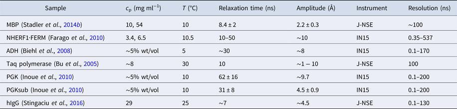
This section is organized as follows: first, a brief summary of the results obtained on the dynamics of hydrated protein powders will be given, and some recent results will be shortly reviewed in the ‘Dynamics of hydrated protein powders’ section. Second, the main studies pointing out differences of protein internal dynamics in hydrated powders compared with solutions will be reviewed in the ‘From powder to solution: influence of solution conditions on protein dynamics’ section. Subsequently, studies regarding a temperature-dependent dynamical transition in solution will be reviewed in the ‘The dynamical transition in solution’ section, followed by studies on the influence of the protein conformation on the internal macromolecular motions in the ‘Comparison of internal protein dynamics in native, molten and denatured states’ and ‘Relations of protein dynamics to structure: from globular to intrinsically disordered proteins’ sections. In the ‘Internal dynamics of proteins at high pressure’ section, pressure experiments on protein solutions are reported. In the ‘Adaptation of proteins to ambient and extreme temperatures’ section, investigation of the molecular basis of thermal adaptation will be reviewed, part of which were performed in vivo. Studies on slow, collective dynamics of domains and subdomains are presented in the ‘Collective internal motions in proteins’ section, and in the ‘Combination of neutron spectroscopy techniques: alcohol dehydrogenase’ section, the characterization of the internal dynamics of alcohol dehydrogenase (ADH) from the fast self-dynamics, to the slow collective dynamics is reviewed. Finally, further in vivo studies are presented in the ‘In vivo neutron spectroscopy’ section, followed by a review of results regarding protein diffusion, in the ‘In vitro studies on the effect of macromolecular crowding on protein dynamics’ and ‘Dynamics of protein clusters, aggregates and glasses’ sections.
Dynamics of hydrated protein powders
Several neutron scattering experiments focused on hydrated protein powders with the aim of suppressing the diffusive dynamics of the entire protein. As a first step toward protein dynamics in solutions, in this section we review some of these studies with the aim to give an overview of the kind of information that can be obtained from such experiments.
Numerous studies have investigated protein internal dynamics on subnanosecond timescales by comparing dry and hydrated protein powders, i.e. with a layer of hydration on the protein surface (for extensive reviews also highlighting the fundamental connection between water and protein structure and dynamics see Daniel et al. (Reference Daniel, Dunn, Finney and Smith2003); Gabel et al. (Reference Gabel, Bicout, Lehnert, Tehei, Weik and Zaccai2003); Halle (Reference Halle2004); Pieper and Renger (Reference Pieper and Renger2009); Khodadadi and Sokolov (Reference Khodadadi and Sokolov2015); Bellissent-Funel et al. (Reference Bellissent-Funel, Hassanali, Havenith, Henchman, Pohl, Sterpone, van der Spoel, Xu and Garcia2016); Khodadadi and Sokolov (Reference Khodadadi and Sokolov2017); Magazù et al. (Reference Magazù, Mezei, Falus, Farago, Mamontov, Russina and Migliardo2017)). Notably, neutron studies have shown that the presence of one hydration water layer activates specific internal motions above a transition temperature T 0 that are not visible in dry samples, thereby confirming Mössbauer spectroscopy results (Parak et al., Reference Parak, Knapp and Kucheida1982). Such an activation is indicated in elastic incoherent neutron scattering (EINS) experiments by the change of the slope of the MSD as a function of temperature, as shown in Fig. 12. This so-called dynamical transition, in some cases, appears correlated with the onset of the protein activity (Fitter et al., Reference Fitter, Ernst, Hauß, Lechner, Hofmann and Dencher1998; Lehnert et al., Reference Lehnert, Réat, Weik, Zaccai and Pfister1998; Réat et al., Reference Réat, Patzelt, Ferrand, Pfister, Oesterhelt and Zaccai1998; Zaccai, Reference Zaccai2000, Reference Zaccai2003). Moreover, it was found to be correlated with an increased mobility of water above T 0 (Tournier et al., Reference Tournier, Xu and Smith2003). Later, Frauenfelder et al. (Reference Frauenfelder, Chen, Berendzen, Fenimore, Jansson, McMahon, Stroe, Swenson and Young2009) explained the experimental observations obtained with Mössbauer spectroscopy proposing a model, in which the localized internal dynamics is strictly entangled with the β-fluctuations of the protein hydration shell. The increased mobility above T ~ 200 K was explained as a result of the changes in the β-relaxations combined with the sensitivity of the experimental technique. Hence, the fact that the dynamical transition, as observed by neutron scattering, does not require a protein structure (He et al., Reference He, Ku, Knab, Chen and Markelz2008) (see also section ‘The dynamical transition in solution’), and occurs even in hydrated amino acids that are not connected in a chain (Schiro et al., Reference Schiro, Caronna, Natali, Koza and Cupane2011) is possibly to be interpreted in light of this model.
Average mean-square displacements  $ \langle u^2 \rangle $ of hydrogen atoms in Mb hydrated powder. Figure adapted and reproduced with permission from Doster et al. (Reference Doster, Cusack and Petry1989). Copyright Nature Publishing Group.

A further study by Nickels et al. (Reference Nickels, O'Neill, Hong, Tyagi, Ehlers, Weiss, Zhang, Yi, Mamontov, Smith and Sokolov2012) employed NBS to access the picosecond-to-nanosecond dynamics of green fluorescent protein (GFP) and its hydration water, revealing that hydration water suppresses protein motions at  $T{\rm \lesssim} 200\,{\rm K}$, and facilitates protein dynamics at higher temperatures. Moreover, a decoupling of the dynamics of hydration water from that of the protein was reported at higher temperatures. Hence, the dynamical transition seen in hydrated powder seems to be slaved to the hydration water, but we anticipate that this is not always observed in solution (see section ‘The dynamical transition in solution’). Finally, the authors found a reduced dynamics of GFP compared with that of other globular proteins from earlier studies and attributed it to the β-barrel structure of GFP.
Sakai et al. (Reference Sakai, Khodadadi, Cicerone, Curtis, Sokolov and Roh2013) explored the influence of water, glycerol and trehalose on the picosecond–nanosecond dynamics of lysozyme using neutron scattering. The data suggested that at room temperature or above, trehalose forms hydrogen bonds with the protein surface, replacing the water molecules, and building a glassy layer suppressing protein dynamics and improving the protein stability (Sakai et al., Reference Sakai, Khodadadi, Cicerone, Curtis, Sokolov and Roh2013). At lower temperatures, instead, it was found that glycerol forms a strong glass integrated with protein residues, which results in suppressed fast motions in the glassy state. In contrast, trehalose interacts only weakly with the protein surface at low temperatures – consistent with arguments based on DSC glass temperature measurements (Olsson et al., Reference Olsson, Jansson and Swenson2016) – and has no stabilizing effect (Sakai et al., Reference Sakai, Khodadadi, Cicerone, Curtis, Sokolov and Roh2013). Hence, the authors concluded that glycerol is the most effective bioprotectant for low temperatures and trehalose for high temperatures.
In an attempt to obtain further insight into the physics behind the increase of the MSD with rising temperature, Zaccai (Reference Zaccai2000) proposed to model proteins in a simplified picture of atoms connected by effective springs. In this picture, the apparent vibrational mean square displacements  $\langle u^2 \rangle $ measured by elastic neutron scattering could be interpreted in terms of the harmonic spring equation, yielding the mean force constant (Zaccai, Reference Zaccai2000)
 $${\langle k \rangle} = 2\,k_{\rm B}\,\left( {\displaystyle{{{\rm d}\langle{u^2} \rangle} \over {{\rm d}T}}} \right)^{-1}$$
with the Boltzmann constant k B. The force constant was associated with the resilience of the protein, and was calculated in a number of studies to compare in a quantitative manner EINS results from different proteins in various conditions (Gabel et al., Reference Gabel, Bicout, Lehnert, Tehei, Weik and Zaccai2003).
Zaccai et al. (Reference Zaccai, Natali, Peters, Řihová, Zimmerman, Ollivier, Combet, Maurel, Bashan and Yonath2016) investigated both water dynamics and conformational fluctuations in the 30 S and 50 S ribosomal subunits from Haloarcula marismortui, under high salt, stable conditions. Whereas no significant difference was observed for hydration water of the two subunits, the 30 S was found to have a softer force constant (0.016(1) and 0.018(2) N m−1 in 3 M NaCl and 3 M KCl, respectively) and larger MSD (17.9(9) and 16.3(8) Å2) than the 50 S ( $\langle k \rangle $ = 0.034(4) N m−1, $\langle u^2 \rangle $ = 12.1(6) Å2). The authors argued that the enhanced flexibility likely facilitates conformational adjustments required for messenger and transfer RNA binding (Zaccai et al., Reference Zaccai, Natali, Peters, Řihová, Zimmerman, Ollivier, Combet, Maurel, Bashan and Yonath2016).
Fabiani et al. (Reference Fabiani, Stadler, Madern, Koza, Tehei, Hirai and Zaccai2009) combined circular dichroism (CD), neutron and X-ray scattering to study changes of MD of apomyoglobin (apoMb) as a function of temperature. A dynamical transition at about 200 K for motions on the 50 ps timescale was observed also for a hydrated powder of heat-denatured aggregated apoMb. Moreover, a significant change in MD indicating a more resilient structure was observed at about 328 K, above which α-helix secondary structure of apoMb at pH 9 was replaced by β-sheet structures, as seen by CD. Such structural changes, confirmed by X-ray scattering, can generate amyloid deposits in humans (Fabiani et al., Reference Fabiani, Stadler, Madern, Koza, Tehei, Hirai and Zaccai2009). These results were later on confirmed by Stadler et al. (Reference Stadler, Pellegrini, Johnson, Fitter and Zaccai2012b), who, in addition, found evidence for amyloid formation and noted that the dynamic changes observed in the α–β transition were more important on the nanosecond timescale, than on the 0.1 ns timescale. Hence, it was suggested by the authors that the secondary structure has a stronger influence on the longer timescale (Stadler et al., Reference Stadler, Pellegrini, Johnson, Fitter and Zaccai2012b).
With regard to Mb, Stadler et al. (Reference Stadler, Garvey, Bocahut, Sacquin-Mora, Digel, Schneider, Natali, Artmann and Zaccai2012c) found different dynamics of hydrated powders of holomyoglobin (holoMb) compared with apoMb: the resilience of holoMb was found to be significantly lower than that of apoMb, indicating entropic stabilization by a higher degree of conformational sampling. The experimental results were further corroborated by MD simulations indicating that, although the residues close to the heme group in the holoMb have a lower MSD, the binding of heme increases the MSD of the other residues, thus providing an entropic contribution to the protein stability.
Andersson et al. (Reference Andersson, Martinez, Zeller, Rondahl, Koza, Frick, Ekström, Peters and Linusson2017) investigated the effect of two different inhibitors, namely TPCK and chymostatin, on the dynamics of the serine protease α-chymotrypsin. From the analysis of the EINS signal, the authors concluded that the inhibited enzymes underwent a dynamical transition at lower temperatures and in a more cooperative way leading to bigger amplitudes of motions at higher temperatures (up to 310 K). Andersson and collaborators deduced that the inhibitor either directly allows for larger amplitudes of the enzyme motions, or influences the water network around the enzymes in a way that permits more degrees of motional freedom leading to a lowering of the potential energy barrier seen by the enzyme atoms (Andersson et al., Reference Andersson, Martinez, Zeller, Rondahl, Koza, Frick, Ekström, Peters and Linusson2017).
Dynamical differences between distinct states of a protein characterized by the presence or absence of a ligand were also investigated by Shrestha et al. (Reference Shrestha, Perera, Bhowmik, Chawla, Mamontov, Brown and Chu2016), who employed neutron scattering to study the activation of the membrane protein rhodopsin. They found a broadly distributed relaxation of hydrogen atom dynamics of rhodopsin on a pico- to nano-second timescale as only observed for globular proteins previously. Moreover they found that the dynamics of opsin, yielded after removal of the ligand 11-cis-retinal through photon absorption, is significantly slower than that of the dark state rhodopsin (before photoactivation), which, instead, is locked by the ligand. This, suggested the authors, may be crucial for functional interactions between opsin and the G-protein transducin leading to its catalytic activation.
Lenton et al. (Reference Lenton, Grimaldo, Roosen-Runge, Schreiber, Nylander, Clegg, Holt, Härtlein, Sakai, Seydel and Teixeira2017) studied the effect of phosphorylation on a disordered protein, the recombinant human-like osteopontin (rOPN). While no significant structural changes could be detected by small-angle X-ray scattering (SAXS), NBS and TOF-NBS showed differences between the dynamics of the phosphorylated and unphosphorylated rOPN. In particular, it was concluded by the authors that phosphorylation of rOPN blocks some nanosecond side-chain motions while increasing the flexibility of other side-chains on faster timescales. Lenton and collaborators suggested that such a selective change of the dynamic behavior of even a highly disordered protein such as osteopontin could direct allosteric mechanisms, interactions with substrates, cofactors and amorphous or crystalline biominerals (Lenton et al., Reference Lenton, Grimaldo, Roosen-Runge, Schreiber, Nylander, Clegg, Holt, Härtlein, Sakai, Seydel and Teixeira2017).
Notably, Hong et al. (Reference Hong, Jain, Cheng, Bernal, Tyagi and Smith2016) performed NBS and NSE experiments on perdeuterated powder of the protein cytochrome P450cam (CYP101) and were able to obtain a description of even large-scale dynamic modes, thereby establishing a microscopic relationship between the structure, dynamics and function. In particular, both experiments and simulations indicated that in CYP101 three domains rotate against each other to grant access of the substrate to the catalytic site, with an amplitude of about 0.4 Å2, which is crucial for the enzymatic function.
In summary, while studies on proteins in hydrated powders generally fail to consider the full dynamical spectrum including center of mass and large scale motions, they highlight the presence of a temperature-activated dynamical transition in the sub-nanosecond internal dynamics. The transition was found to be coupled to the dynamics of the hydration water, and, in some cases, it was possible to associate the onset of the fast dynamics with the activation of the protein function. Recent studies on protein powders have also shown that distinct ribosomal subunits are characterized by different mean effective force constants. Experiments further demonstrated that binding of ligands and phosphorylation can induce changes in the protein dynamics and suggested that the secondary structure of proteins may have a stronger influence on nanosecond internal dynamics than on shorter timescales. Finally, a perdeuterated powder of CYP101 was successfully used to obtain a description of even large-scale dynamic modes.
General features of the dynamics of proteins in solution as seen by neutron scattering
As a general remark on the parameters measured by neutron scattering (cf. Table 4), we note that the effective force constants of proteins in solution in vitro span from some piconewtons per nanometer (10−3 N m−1), to some hundreds of piconewtons per nanometer (10−1 N m−1), with the exception of Methanococcus jannaschii malate dehydrogenase (Mj MalDH), having 〈k〉=1.5 N m−1. In particular, force constants measured on the 10 ps timescale are mostly on the order of 10−2 N m−1. Those measured on a 100 ps timescale are predominantly on the order of some 10−1 N m−1, while on the longer timescales of some nanoseconds and some hundreds of nanoseconds, effective force constants appear to decrease to some 10−2 N m−1 and even some 10−3 N m−1, as obtained from models of the full NBS and NSE signals, respectively.
QENS studies (cf. Table 5) suggest that the radius R of the effective sphere accessible by H-atoms within a protein close to room temperature vary from ~1.5 to ~7 Å, whereas the internal relaxation times τ are more heterogeneous, spanning from some picoseconds to some hundreds of picoseconds, depending on the instrument resolution. These relaxation times can be compared with typical ‘fast’ rotational correlation times on the order of some hundreds of picoseconds in native proteins, as observed for specific residues by fluorescence spectroscopy (Lakshmikanth and Krishnamoorthy, Reference Lakshmikanth and Krishnamoorthy1999; Mukhopadhyay et al., Reference Mukhopadhyay, Nayak, Udgaonkar and Krishnamoorthy2006; Mondal et al., Reference Mondal, Kallianpur, Udgaonkar and Krishnamoorthy2015), and residue-specific internal relaxation times ranging from a few tens to some hundreds of picoseconds in the same protein, as generally observed by NMR (Stone et al., Reference Stone, Chandrasekhar, Holmgren, Wright and Dyson1993; Wand et al., Reference Wand, Urbauer, McEvoy and Bieber1996; Constantine et al., Reference Constantine, Friedrichs, Wittekind, Jamil, Chu, Parker, Goldfarb, Mueller and Farmer1998; Hill et al., Reference Hill, Bracken, DeGrado and Palmer2000; Ishima et al., Reference Ishima, Petkova, Louis and Torchia2001; Skrynnikov et al., Reference Skrynnikov, Millet and Kay2002). The former represent the local motional freedom of the covalently bound probe with respect to the polypeptide chain, the latter are due either to methyl reorientational and other motions of side-chains bearing methyl groups, or to backbone fluctuations.
The fraction of atoms seen as immobile by QENS on the 10–100 ps time is generally about 0.6, while it ranges from ~0.1 to ~0.2 on the nanosecond timescale. Finally, the internal collective dynamics as measured by NSE (cf. Table 6) is characterized by relaxation times ranging from several nanoseconds to several tens of nanoseconds and amplitudes of several Ångströms.
From powder to solution: influence of solution conditions on protein dynamics
Motivated by the different states of powder samples and protein solutions, several studies focused on the subnanosecond internal dynamics of protein powders under different hydration conditions and in solution. After reviewing these studies, results on the influence of the specific solvent conditions (use of H2O versus D2O, presence of salts) on protein dynamics are summarized.
In 1999, Pérez and co-workers performed the first systematic neutron scattering experiments on the picosecond internal dynamics of proteins as a function of hydration, from dry powders to solutions (Pérez et al., Reference Pérez, Zanotti and Durand1999). Measurements of two proteins, Mb and lysozyme (Lys), demonstrated that, from dry powder to coverage by one water layer, the surface side-chains progressively participate in local diffusive motions. The half-widths at half-maxima, Γ, of the Lorentzian function  $\cal L $(Γ, ω) accounting for the internal dynamics of the proteins in hydrated powders and solutions are shown in Fig. 13. When increasing the level of hydration, the rate of the local proton diffusion is enhanced. In a solution with ~60 mg ml−1 protein, motions were found to occur with an average amplitude larger than in the fully hydrated powder by about a factor three. Also, the calculated average relaxation time decreased from ~9.4 ps in powders with one hydration layer to ~4.5 ps in solution.
HWHM, Γ, of the internal motion Lorentzian L(Γ, ω), for Mb samples. The lines are guide to the eye. Except for the dry Mb sample, Γ increases with q 2, which characterizes the presence of local diffusive motions as soon as the protein is hydrated. In the case of dry Mb, Γ is almost constant, as expected from a reorientational type of motion. The inverse of Γ gives the correlation time of the motions. In solutions, the correlation time extrapolated at q = 0 is ~4.4 ps, less than half of that in powders. Figure adapted and reproduced with permission from Pérez et al. (Reference Pérez, Zanotti and Durand1999). Copyright Elsevier.

The authors also noticed that, in solution, a component of the total scattering characterized by a quasi-elastic broadening proportional to q 2 (typical for Fickian diffusion) could be attributed to the global diffusion of the entire proteins, including both a translational and a rotational contribution. Importantly, the contribution of rotational diffusion to the apparent diffusion coefficient measured by QENS was calculated and the translational coefficient could be consistently extracted from the data (Pérez et al., Reference Pérez, Zanotti and Durand1999).
Shortly after this first systematic study, differences between the dynamics of a hydrated powder (0.4 g D2O per g protein) and a solution (50 mg ml−1) of α-amylase from Bacillus licheniformis were investigated by Fitter (Reference Fitter2000) with a similar energy resolution. Clear differences were observed between the two types of samples. In particular, the number of mobile atoms was found to increase significantly, whereas the volume accessible to the atoms was reported to decrease. We remark that here any contribution arising from global diffusion was neglected (Fitter, Reference Fitter2000).
In a comparative neutron scattering study of the dynamics of Lys in hydrated powders and in solutions at ~100 mg ml−1, a two-power law characteristics of the quasi-elastic contribution to the spectra was identified, with a ballistic Gaussian decrease above ~2 meV (Marconi et al., Reference Marconi, Cornicchi, Onori and Paciaroni2008). The most significant difference between the powder and the solution sample was the much larger intensity of the quasi-elastic contribution, which was attributed by the authors to the increase of both the number and the amplitudes of the confined diffusive processes related to protein side-chain motions at the protein surface (Marconi et al., Reference Marconi, Cornicchi, Onori and Paciaroni2008). The comparison confirmed thus that proteins in solution exhibit enhanced dynamics.
Further investigations focused on the effect of an increasing hydration level and on the difference between the dynamics in powders and solution (Jansson et al., Reference Jansson, Kargl, Fernandez-Alonso and Swenson2009; Russo et al., Reference Russo, Teixeira and Ollivier2009; Stadler et al., Reference Stadler, Digel, Embs, Unruh, Tehei, Zaccai, Büldt and Artmann2009). Jansson et al. (Reference Jansson, Kargl, Fernandez-Alonso and Swenson2009) employed NBS to study Mb in water:glycerol mixtures at hydration levels ranging from h = 0.5 to 2 g solvent per g protein, in a temperature range of 260–320 K. The data were fitted with a single KWW function (see section ‘Localized internal dynamics’). The results suggested that the stretched nature of the correlation functions is due to a distribution of exponential relaxations with different relaxation times rather than to a homogeneous non-exponential relaxation, but were also consistent with the assumption that the protein dynamics is dominated by confined motions on the accessible timescale. Jansson et al. (Reference Jansson, Kargl, Fernandez-Alonso and Swenson2009) investigated the dynamics of the solvent, which was well described by a jump-diffusion model, with the jump-diffusion coefficients being a factor 2.0 ± 0.3 and 2.6 ± 0.3 slower than for bulk water, for h = 1 and h = 0.5, respectively. Moreover, they found temperature dependences of the protein average relaxation times very similar to that of the average solvent relaxation times. The absolute values, however, were found to be significantly different, those of the protein atoms being in a range of ~1–10 ps, and those of the solvent in a range of ~5–30 ps. Hence, the data were consistent with the hypothesis of a slaving of the protein dynamics to the solvent, but at the same time the authors noted that the protein dynamics was strongly dependent on the hydration level, implying that also the amount of solvent plays an important role in the activation of protein internal relaxations (Jansson et al., Reference Jansson, Kargl, Fernandez-Alonso and Swenson2009).
Russo et al. (Reference Russo, Teixeira and Ollivier2009, Reference Russo, Hura and Copley2007) measured the internal dynamics of hydrophobic side-chains of small peptides as a function of the level of hydration and of temperature. Hydrated powders were measured from 50 to 300 K, whereas the solutions were measured between 275 and 310 K. An evolution of the dynamics was observed: for low levels of hydration, only rotational motions, mostly due to methyl group rotations were observed, whereas at high hydration levels also translational internal diffusive motions were detected above 250 K. Importantly, the experiments revealed that only long side-chains could trigger the diffusive motion, while short side-chains were found to undergo only rotational motions. Therefore, both the interfacial water and the side-chain length play a major role in the dynamical transition (Russo et al., Reference Russo, Teixeira and Ollivier2009). Surprisingly, the internal translational motions were not observed in highly concentrated solutions at room temperature (Russo et al., Reference Russo, Hura and Copley2007), but were only measured in hydrated powders (Russo et al., Reference Russo, Teixeira and Ollivier2009). This discrepancy was explained as a consequence of the structural and dynamical properties of the specific interfacial water network, since the hydration water network around hydrophobic side-chains in hydrated powders is less structured (Russo et al., Reference Russo, Teixeira and Ollivier2009). Therefore, the outcome of the experiment corroborated the hypothesis of the authors that protein dynamics is strongly influenced by the structural and dynamical properties of interfacial water (Russo et al., Reference Russo, Teixeira and Ollivier2009). No significant differences between different hydration levels were reported at low temperatures (T <250 K) (Russo et al., Reference Russo, Teixeira and Ollivier2009).
Stadler et al. (Reference Stadler, Digel, Embs, Unruh, Tehei, Zaccai, Büldt and Artmann2009, Reference Stadler, Fabiani and Zaccai2012a) focused on the internal picosecond dynamics of human Hb, as well as platypus and chicken Hb, as a function of hydration and temperature. The rates of the diffusive motion were found to increase with increasing hydration up to highly concentrated solutions (~570 mg ml−1). Moreover, the data showed a substantial difference between powders and solutions: in solution, the volume accessible to the amino acid side-chains above body temperature was larger than that expected from a linear extrapolation from lower temperatures. The same was not observed in fully hydrated powders, suggesting that the investigation of fully hydrated protein powders is not sufficient to accurately describe all aspects of protein picosecond dynamics that might be relevant for biological function (Stadler et al., Reference Stadler, Digel, Embs, Unruh, Tehei, Zaccai, Büldt and Artmann2009).
Before concluding this section we note that the amplitude of fast molecular motions depends on the properties of the solvent, such as on whether the protein is dissolved in H2O or in D2O, and on the presence of different kinds of salts or cosolvents. This phenomenon was measured with elastic neutron scattering in solutions of halophilic MalDH, and bovine serum albumin (BSA) at ~200 mg ml−1 (Tehei et al., Reference Tehei, Madern, Pfister and Zaccai2001), as well as for full cells of Escherichia coli (Jasnin et al., Reference Jasnin, Tehei, Moulin, Härtlein and Zaccai2008b). The values of resilience measured in the study can be found in Table 4, and the overall cytoplasm shows a smaller motional amplitude and smaller resilience in D2O compared with H2O (Jasnin et al., Reference Jasnin, Tehei, Moulin, Härtlein and Zaccai2008b). It was noted by Tehei et al. (Reference Tehei, Madern, Pfister and Zaccai2001) that BSA must be stabilized predominantly by entropic effects, since its resilience is higher in H2O, even though its thermostability is higher in D2O. In contrast, the higher resilience of MalDH in D2O, where the protein is more stable, suggests that enthalpic terms dominate its stability (Tehei et al., Reference Tehei, Madern, Pfister and Zaccai2001). The ion-dependent changes of k in MalDH were interpreted as a consequence of a significant contribution of the protein–ion interactions in the hydration shell. Hence, although the use of D2O is common praxis for neutron scattering, NMR, and other spectroscopic techniques, it should be kept in mind that the solvent affects protein dynamics in a non-trivial way (Tehei et al., Reference Tehei, Madern, Pfister and Zaccai2001) and the quantitative determination of some parameters related to the protein structure and dynamics may differ depending on whether the protein is dissolved in H2O or in D2O (Gabel et al., Reference Gabel, Bicout, Lehnert, Tehei, Weik and Zaccai2003).
Al-Ayoubi et al. (Reference Al-Ayoubi, Schummel, Golub, Peters and Winter2017) further found that two different cosolvents in D2O, namely trimethylamine-N-oxide (TMAO) and urea, affect the sub-nanosecond dynamics in different ways. At ambient pressure, the presence of 2 M TMAO in a solution of Lys at concentrations of 80 and 160 mg ml−1 in D2O results in the MSD being reduced by  $\sim 70\% $ and $\sim 45\% $ respectively, compared with Lys in pure D2O. Instead, 2 M urea was found to reduce the MSD by only $\sim 35\% $ in the most diluted sample and to have no effect on the most concentrated one. Finally, a urea–TMAO 2–1 M mixture caused a reduction of the MSD by $\sim 75\% $ in the 80 mg ml−1 Lys sample. At higher pressures, the MSD values in the presence and absence of urea were found to be of similar magnitude at both protein concentrations, and in general the MSD remains rather constant over the whole pressure range probed in the presence of both cosolvents (Al-Ayoubi et al., Reference Al-Ayoubi, Schummel, Golub, Peters and Winter2017) (see also section ‘Internal dynamics of proteins at high pressure’). Additional Fourier-transform IR spectroscopy indicated a stabilization effect of the osmolyte TMAO and a destabilization in the presence of urea. The authors hypothesized that the different influences of TMAO and urea be due the fact that urea interacts weakly with water, but directly with the protein-backbone, while TMAO is preferentially excluded from the protein surface and instead enhances the overall hydrogen bonding network structure. The authors speculate that this might lead to a damping of conformational fluctuations of the protein's surface groups which propagates into the protein interior, thereby affecting the flexibility of the whole protein molecule (Al-Ayoubi et al., Reference Al-Ayoubi, Schummel, Golub, Peters and Winter2017).
In conclusion, a general outcome of the reported neutron scattering experiments is that additional MD is found when proteins are in solution, compared with hydrated powders, as schematically depicted in Fig. 14. A similar result was obtained in a recent NMR study (Harpole et al., Reference Harpole, O'Brien, Clark, McKnight, Vugmeyster and Wand2016) highlighting how the dynamics faster than ~3 ns of methyl-bearing side-chains in solution is clearly different from that in hydrated powders (~0.4 g water per g protein), for which in turn a change of dynamics was detected by NMR (Separovic et al., Reference Separovic, Lam, Ke and Chan1998; Diakova et al., Reference Diakova, Goddard, Korb and Bryant2007; Krushelnitsky et al., Reference Krushelnitsky, Zinkevich, Mukhametshina, Tarasova, Gogolev, Gnezdilov, Fedotov, Belton and Reichert2009) and dielectric relaxation spectroscopy (Mijovic et al., Reference Mijovic, Bian, Gross and Chen2005; Khodadadi et al., Reference Khodadadi, Pawlus and Sokolov2008; Fomina et al., Reference Fomina, Schirò and Cupane2014) as a function of hydration. Further NMR studies, instead, indicated that the dynamics of both methyl groups (Reif et al., Reference Reif, Xue, Agarwal, Pavlova, Hologne, Diehl, Ryabov and Skrynnikov2006; Agarwal et al., Reference Agarwal, Xue, Reif and Skrynnikov2008) on the sub-nanosecond timescale and backbone atoms (Chevelkov et al., Reference Chevelkov, Xue, Linser, Skrynnikov and Reif2010) on a ~1–100 ns timescale is mostly unchanged, when comparing proteins in crystals and aqueous solution, consistent with the observation that, in hydrated powders, the millisecond-dynamics does not change significantly above ~0.3 g g−1, at least up to h ~0.7 g water per g protein (Krushelnitsky et al., Reference Krushelnitsky, Zinkevich, Mukhametshina, Tarasova, Gogolev, Gnezdilov, Fedotov, Belton and Reichert2009).
Sketch of the gradual dynamics activation from protein powders to proteins in solution. Numerous studies indicate that, generally, additional dynamics is present in proteins in solution compared with hydrated protein powders, which in turn are characterized by additional types of motions compared with dry protein powders. IgG (Harris et al., Reference Harris, Larson, Hasel and McPherson1997) was rendered using PyMol (DeLano, Reference DeLano2002) and the figure was produced with Gimp (Spencer Kimball and the GIMP Development Team).
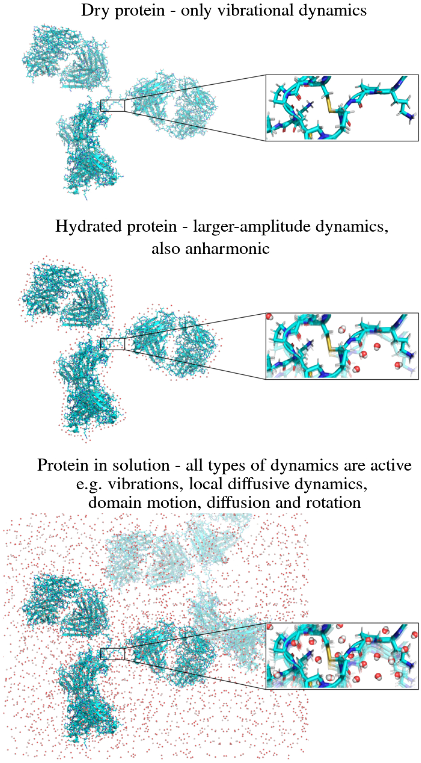
Nevertheless, the additional sub-nanosecond dynamics observed mostly by neutron scattering in solution can be relevant for biological function (for more general information on the hydration–function relation, see e.g. Ball (Reference Ball2008)), and hence a full picture of the dynamical properties of proteins does require studies in solution. In this context, it was established that, after appropriate sample preparation, information on the internal dynamics can be detected by neutron scattering experiments also in bulk solutions composed of membrane proteins in detergent microemulsions (Gall et al., Reference Gall, Seguin, Robert and Bellissent-Funel2002).
Finally, it should be kept in mind that marked differences in the amplitude of protein fluctuations can occur depending on the solvent. Although no general understanding could be presented so far, recent studies suggest that the hydrogen bonding network around the protein surface might play a role in this respect.
The dynamical transition in solution
A dynamical transition at low T far below physiological temperatures was observed in protein hydrated powders in numerous studies, as briefly mentioned in the ‘Dynamics of hydrated protein powders’ section (for a review see those by Gabel et al. (Reference Gabel, Bicout, Lehnert, Tehei, Weik and Zaccai2003) and Daniel et al. (Reference Daniel, Dunn, Finney and Smith2003)). In aqueous solutions, similar measurements are limited by the crystallization of water. Nevertheless, few experiments, mostly on proteins dissolved in antifreeze solvents (cryoprotectants), revealed a dynamical transition also in solution. Such studies are presented below.
Neutron scattering experiments probing two different timescales, namely below 100 ps, as seen by TOF, and below 5 ns, as seen by NBS, were performed on solutions of the enzyme glutamate dehydrogenase in 70% v/v CD3OD/D2O for 70 K<T <320 K (Daniel et al., Reference Daniel, Smith, Ferrand, Hry, Dunn and Finney1998, Reference Daniel, Finney, Réat, Dunn, Ferrand and Smith1999). The temperature dependence of the MSD was found to be markedly dependent on the instrument resolution: at the nanosecond timescale, several inflections of the MSD were identified, at ~140, ~210 and 280 K, while on the picosecond timescale only the well-known dynamical transition at ~220 K was observed. Moreover, none of these temperatures could be associated with an activity loss. It was therefore concluded that anharmonic fast motions are not necessarily coupled to the much slower motions required for the enzyme activity. However, as noted by the same authors, it cannot be excluded that functionally important fast motions may occur locally in the protein at the active site, even though these are not detectable in the average dynamics (Daniel et al., Reference Daniel, Finney, Réat, Dunn, Ferrand and Smith1999).
Another investigation regarding the dynamical transition in protein solutions was carried out by Réat et al. (Reference Réat, Dunn, Ferrand, Finney, Daniel and Smith2000). The study focused on the solvent dependence of the picosecond dynamic transition of solutions of xylanase, a simple single-subunit enzyme. The elastic intensity of the protein in dry powder, in D2O, and in four two-component perdeuterated single-phase cryosolvents in which the protein is active and stable was measured with a resolution of 50 eV. It was found that the dynamic transitions of the protein solutions are partially coupled to those of the respective solvents. In D2O a very sharp transition is observed at ~280 K, i.e. substantially above the transition temperature of hydrated powders (200–220 K), but very close to the melting temperature of D2O, T m = 277 K. In the cryosolvents used in the performed experiment, instead, the transition is much more gradual and starts at ~230 K, independent of the cryosolvent composition. In particular, the transition temperature remains the same not only in the cryosolvent with a melting temperature of ≈ 230 K, but also in that with melting temperature below 190 K (Réat et al., Reference Réat, Dunn, Ferrand, Finney, Daniel and Smith2000).
An at least apparent decoupling of the dynamics of a protein (Lys) in solution from the dynamics of its solvent (7.6 M LiCl D2O) was observed also in a more recent QENS study (Chu et al., Reference Chu, Mamontov, O'Neill and Zhang2012). Other than the cryosolvent used in the aforementioned study, which was characterized by a melting point below 190 K (Réat et al., Reference Réat, Dunn, Ferrand, Finney, Daniel and Smith2000), the LiCl solution undergoes a dynamical crossover at about 220 K. Nevertheless, no transition is visible in the protein dynamics at this temperature. The authors argued that there may be two ways to explain the observations: (i) there is a real decoupling of the dynamics of the solvent from that of the protein, or (ii) the transition observed for the solvent does not reflect a transition in its α-relaxation, which is believed to drive the dynamical transition in proteins (Chu et al., Reference Chu, Mamontov, O'Neill and Zhang2012).
The protein dynamical transition in solution was further observed by terahertz dielectric spectroscopy by Markelz et al. (Reference Markelz, Knab, Chen and He2007) and He et al. (Reference He, Ku, Knab, Chen and Markelz2008), in comparison with MD simulations. Such investigations, as opposed to the ones reported above, revealed that, on the sub-picosecond timescale, the dynamical transition of native and denatured proteins as well as polypeptides dissolved in H2O occurs at about 200 K (the same temperature observed for hydrated powders), independent of the protein secondary and tertiary structure and concentration (He et al., Reference He, Ku, Knab, Chen and Markelz2008). Hence, this study first revealed that the dynamical transition on the sub-picosecond timescale does not require a protein structure, but is probably rather due to the side-chain interaction with the solvent. He et al. (Reference He, Ku, Knab, Chen and Markelz2008), however, provide evidence using a phonon-assisted Mössbauer experiment on hydrated powders (Achterhold et al., Reference Achterhold, Keppler, Ostermann, Van Bürck, Sturhahn, Alp and Parak2002) that such a transition on the sub-picosecond timescale does not concern the protein core.
Summarizing, neutron as well as terahertz spectroscopy experiments show that the dynamical transition is not restricted to protein hydrated powders, but can be observed also in D2O, H2O and cryosolvents. Unlike for hydrated powders, the coupling of the protein dynamics and the dynamics of the solvent at low temperature (when using cryosolvents) does not seem to be obvious.
For proteins in (heavy) water, the combination of results from THz spectroscopy and neutron scattering suggests the following picture. The water-side-chain interaction suppresses water crystallization on the protein surface except for short chain lengths, as reflected by the transition at ~200 K of the sub-picosecond dynamics probed by THz spectroscopy (Markelz et al., Reference Markelz, Knab, Chen and He2007; He et al., Reference He, Ku, Knab, Chen and Markelz2008). The suppression of water crystallization, however, is probably still insufficient to trigger motions on the picosecond to nanosecond timescale, or it affects too few side-chains to be observed by neutron scattering. Instead, significant movements on these timescales seem to require the melting of a larger fraction of D2O (Réat et al., Reference Réat, Dunn, Ferrand, Finney, Daniel and Smith2000).
Comparison of internal protein dynamics in native, molten and denatured states
Several studies have attempted identifying general differences of the internal dynamics of proteins in solution between well-folded conformations and molten (i.e. an intermediate equilibrium state between native and fully denatured) or unfolded states. In the following, we summarize the results of such investigations.
The comparison of TOF data of yeast phosphoglycerate kinase (PGK) in the native form and denatured in 1.5 M guanidinium chloride revealed a clear increase of the fraction of hydrogen atoms undergoing picosecond diffusive motions upon denaturation (Receveur et al., Reference Receveur, Calmettes, Smith, Desmadril, Coddens and Durand1997). The same experiment evidenced that the H-atoms can access a larger volume in the denatured state, as reflected by the increase of the radius of the effective accessible sphere from 1.8 to 2.2 Å (cf. section ‘Modeling and analysis’).
Partial denaturation through C-terminal truncation of staphylococcal nuclease (snase) was studied in solutions at a concentration c p ~ 80 mg ml−1 by TOF spectroscopy by Kataoka et al. (Reference Kataoka, Ferrand, Goupil-Lamy, Kamikubo, Yunoki, Oka and Smith1999a). An increase in the amplitude of the picosecond-timescale average local fluctuations u 2 on truncation of the 13C-terminal residues of snase was detected, from 0.49 ± 0.02 Å in the native state to 0.60 ± 0.02 Å in the denatured form. MD simulations suggested that these differences are related to an increased solvent accessibility of the protein chain, accompanied by a decrease of the number of internal hydrogen bonds (Kataoka et al., Reference Kataoka, Ferrand, Goupil-Lamy, Kamikubo, Yunoki, Oka and Smith1999a). However, overall, NMR studies probing the sub-nanosecond dynamics of methyl-bearing side-chains in solution showed essentially no correlation between their amplitudes and their depth, their local packing density, or their solvent accessible surface area (Igumenova et al., Reference Igumenova, Frederick and Wand2006). This suggests that the increased amplitude of motion observed by Kataoka et al. (Reference Kataoka, Ferrand, Goupil-Lamy, Kamikubo, Yunoki, Oka and Smith1999a) is rather related to the decrease of the number of internal hydrogen bonds.
Picosecond dynamics differences were also measured between the native bovine α-lactalbumin (BLA) and its molten globules (MBLA) at ~75 mg ml−1 by Bu et al. (Reference Bu, Neumann, Lee, Brown, Engelman and Han2000), as shown in Fig. 15. The authors observed that spatially restricted long-range diffusive motions and local jump motions (cf. section ‘Modeling and analysis’) of H-atoms within the proteins are less restricted in the molten globules than in the native BLA. At T = 303 K, it was found that H-atoms in BLA and MBLA diffuse in effective spheres of radii R BLA = 4.1 ± 0.1 Å and R MBLA = 5.4 ± 0.1 Å, as obtained from the fit of the EISF in Fig. 15a. A jump-diffusion was identified, with diffusion coefficients D BLA = 42 ± 0.5 Å2 ns−1 and D MBLA = 73 ± 0.5 Å2 ns−1, and a residence time τ BLA = 56 ± 7 ps in native BLA, reducing to τ MBLA = 23 ± 2 ps in MBLA (Fig. 15b). However, root mean square jump distances did not change significantly ( $\sqrt {{\langle r^2\rangle} _{{\rm BLA}}} = 3.7 \pm 0.3\,$ Å versus $\sqrt {{\langle r^2\rangle} _{{\rm MBLA}}} = 3.2 \pm 0.3$ Å), which may indicate switching between different rotamers (Bu et al., Reference Bu, Neumann, Lee, Brown, Engelman and Han2000). In addition to the self-dynamics, Bu and co-workers extracted information on collective diffusive motions within the protein (Bu et al., Reference Bu, Neumann, Lee, Brown, Engelman and Han2000). Evaluating the coherent scattering suggested that atoms move in a correlated manner with correlation lengths ξ BLA = 18 ± 4 Å and ξ MBLA = 6.9 ± 1.2 Å respectively. Therefore, the dynamics of the native protein is characterized by more localized motions of atoms correlated up to relatively long distances, as opposed to that of the molten globule presenting less localized motions of less strongly correlated atoms.
(a) EISF of: BLA (black squares) and MBLA (empty circles). Although a better fit to the EISF was achieved with a two-sphere model, the one sphere model (Eq. (40)) was used in Bu et al. (Reference Bu, Neumann, Lee, Brown, Engelman and Han2000) to describe the change in the effective radius of restricted motions. (b) q dependence of HWHM Γ of the quasi-elastic Lorentzian peak of: BLA (black squares) and MBLA (empty circles). Clear differences are visible between the two states of the protein. Figure adapted and reproduced with permission from Bu et al. (Reference Bu, Neumann, Lee, Brown, Engelman and Han2000). Copyright Elsevier.

In a later study, Bu et al. (Reference Bu, Cook and Callaway2001) compared the nanosecond and picosecond dynamics of native, molten and denatured BLA in solution at 60 and ~15 to 20 mg ml−1, respectively. Two dynamical contributions (two Lorentzian functions) were used to describe the TOF data. The fast contribution was identified with the motion of the side-chains, whereas the other one was attributed to the center-of-mass motion of the protein and was not discussed. The picosecond dynamics showed a reduced potential barrier to side-chain torsional motion in the molten globule and in the denatured protein. Importantly, although faster internal dynamics may be expected also because of the lower concentration of the molten and denatured protein samples compared with that of the native protein solution, the urea-denatured BLA showed a less restricted long-range motion than both native protein and the molten globule, the latter at a comparable concentration. Unlike the TOF data, the NBS data were interpreted in terms of one single dynamical contribution, under the assumption that the center-of-mass diffusion was too fast to be detected. The results suggested the presence of dynamical regimes and strongly correlated density fluctuations within the native protein and the denatured states, based on coherent scattering intensity: an unusual dynamical behavior not observed for chain-like polymers was reported, which was suggested to be due to strongly non-local, attractive forces within the proteins. Finally, the analysis of the q-dependence of the scattering intensity suggested that both a residual secondary structure and long-range interactions on the scale of the tertiary structure fluctuate over several hundred picoseconds in both the native protein and in the highly denatured states α-lactalbumin (Bu et al., Reference Bu, Cook and Callaway2001).
BLA in the native and molten state was further studied combining QENS and MD simulations (Tarek et al., Reference Tarek, Neumann and Tobias2003). The protein concentrations were ~60 mg ml−1 for the native and ~20 mg ml−1 for the molten globule. The study confirmed the increase of the average internal motion of the molten state, and showed that such a motion is characterized by a high degree of heterogeneity, which is more pronounced in MBLA compared with BLA. The simulations showed differences of up to an order of magnitude between the amplitude of motions in highly structured parts of the protein, compared with unstructured regions (loops connecting secondary structural elements, termini, unfolded chain segments of the molten globule). Thereby, it was demonstrated that the increased average sub-nanosecond dynamics of the molten globule was mainly due to additional motions in the region of the protein that unfolds upon formation of the molten globule (Tarek et al., Reference Tarek, Neumann and Tobias2003).
The same conclusion was drawn earlier by Russo et al. (Reference Russo, Pérez, Zanotti, Desmadril and Durand2002) in a study on the temperature dependence of the picosecond internal dynamics of an all-β protein, neocarzinostatin, in solutions at 58 and 42 mg ml−1 (Russo et al., Reference Russo, Pérez, Zanotti, Desmadril and Durand2002). The authors observed that the number of protons undergoing detectable diffusive motions increased from 33% at 293 K to ~90% upon heat-induced partial unfolding at 344 K. Furthermore, a decrease of the average volume accessible to the atoms upon unfolding was reported. It was pointed out by the authors of this study that 33% is very close to the fraction of protons contained in the side-chains of random coil structures and it was suggested that, at room temperature, the only detectable diffusive movements are those involving the side-chains of random coil structures. Thus, the increased fraction of mobile atoms at higher temperature could be explained by the onset of picosecond dynamics in the fraction of backbone and β-sheet side-chain hydrogen atoms, which were seen as immobile at room temperature. These atoms would still be in a very confined environment until the protein is fully unfolded, which would account for the decrease of the average accessible volume, as most of the additional motion would have to be very restricted (Russo et al., Reference Russo, Pérez, Zanotti, Desmadril and Durand2002).
Also a later study by Gibrat et al. (Reference Gibrat, Assairi, Blouquit, Craescu and Bellissentfunel2008) on apo-calmodulin reported the observation of a dynamical transition upon protein thermal denaturation. The transition was characterized by a decrease of the confinement of hydrogen atoms, and a decrease of the fraction of immobile protons. Moreover, the data analysis revealed an increase of dynamical heterogeneity, but also a decrease of the ‘most probable volume explored’ (Gibrat et al., Reference Gibrat, Assairi, Blouquit, Craescu and Bellissentfunel2008). It was proposed that the distance between atom and protein backbone is more important for the dynamics than the solvent exposure of the residue, or a related classification of the residue as belonging to the surface or the interior of the protein. In fact, if the exposure of the residue to the solvent determined dynamics, this should be less homogeneous in the folded state, where only a fraction of side-chains is solvent-exposed, than in the unfolded state, where all residues become exposed to the solvent (Gibrat et al., Reference Gibrat, Assairi, Blouquit, Craescu and Bellissentfunel2008). This hypothesis is consistent with previously mentioned NMR observations indicating the absences of correlations between the amplitude of sub-nanosecond dynamics of side-chains containing methyl groups and their solvent accessibility, as well as their depth, and their local packing density (Igumenova et al., Reference Igumenova, Frederick and Wand2006).
An increase of the radius as obtained from the diffusion in a sphere model (cf. section ‘Modeling and analysis’) was observed instead for α-amylase by Fitter (Reference Fitter2003a) at 30 mg ml−1 from the folded (R = 1.2 Å) to a pH-induced unfolded conformation (R = 1.8 Å). In both states, at 303 K, an average correlation time of ~4.4 ps and a mean square displacement  $\langle u^2 \rangle $ = 0.15 ± 0.03 Å2 were found (Fitter, Reference Fitter2003a).
At higher temperatures, while no variation within the experimental error of the correlation time was observed, an increase of R was detected (Fitter, Reference Fitter2003b). Such a change was more pronounced in the unfolded conformation, the radius of which increased from R ≃ 1.8 Å at 303 K to R ≃ 2.4 Å at 343 K, as opposed to that of the native protein, which increased from R ≃ 1.2 Å at 303 K to R ≃ 1.4 Å at 343 K. The conformational entropy change between the two states upon heating was also estimated on the basis of the neutron scattering data and a significant increase upon heating was demonstrated. As a consequence, it was concluded that, since an increasingly larger part of the conformational space can be explored by confined motions with increasing temperature in the unfolded compared with the natively folded protein, the conformational entropy change contributes significantly to thermal unfolding (Fitter, Reference Fitter2003b). This result is consistent with NMR experiments on α-lactalbumin showing that also conformational fluctuations of the backbone on microsecond to millisecond timescales are more strongly enhanced in molten globules than in the native protein when rising temperature (Ramboarina and Redfield, Reference Ramboarina and Redfield2008).
Jansson and Swenson (Reference Jansson and Swenson2008) investigated the dynamical behavior of both the protein Hb and its surrounding water during thermal denaturation using EINS as a support to complement modulated temperature differential scanning calorimetry, and frequency dependent conductivity measurements. Their analysis of the elastic intensity as a function of temperature throughout thermal denaturation suggested that the unfolding of the secondary structure reduces the number of water molecules mobile on a 50–100 ps timescale – probably because of an increased number of water molecules interacting with the larger exposed protein surface –, whereas the flexibility of the protein was found to be enhanced by denaturation. The important role of the solvent properties at the hydration interface in determining the region in the temperature-pressure thermodynamic plane in which proteins are stable, is further demonstrated by multiple experimental and computational studies (Bellissent-Funel et al., Reference Bellissent-Funel, Hassanali, Havenith, Henchman, Pohl, Sterpone, van der Spoel, Xu and Garcia2016; Bianco et al., Reference Bianco, Pagès-Gelabert, Coluzza and Franzese2017).
A combined QENS and EINS study was performed on the thermal denaturation of BSA in highly concentrated aqueous solution (Hennig et al., Reference Hennig, Roosen-Runge, Zhang, Zorn, Skoda, Jacobs, Seydel and Schreiber2012). The apparent mean square displacement u 2 was decomposed into the global diffusive contribution  $u_{{\rm diff}}^2 $ and the internal part $ \langle u^2 \rangle -u_{{\rm diff}}^2 $ comprising the vibrations and the subunit diffusive motions. Upon increasing T, u 2 was characterized by a linear increase up to T = 325 K, followed by a sharp decrease in the range 331 K<T <354 K and a second linear increase up to 370 K. This observation was interpreted as a result of the transition from a liquid solution to a cross-linked gel-like state: as long as the proteins are free, they diffuse increasingly fast with rising temperature. When denaturation starts, the diffusion is hindered by the formation of a growing network. When the formation of the cross-linked network of denatured proteins is complete, a further temperature increase enhances the dynamics of the subunits of the proteins, while their center-of-mass diffusion is restrained. The MSD of the internal dynamics $ \langle u^2\rangle - \langle u_{{\rm diff}}^2 \rangle $ showed a slow linear increase up to the denaturation temperature T = 343 K, after which it increased linearly with a higher slope, indicating an enhanced flexibility after denaturation, consistent with a more marked increase of the average relaxation rate measured by fluorescence spectroscopy on rubredoxin mutant A51C (Santos et al., Reference Santos, Duarte, Fedorov, Martinho and Moura2010) and on human serum albumin (Yadav et al., Reference Yadav, Sengupta and Sen2014) above ~343 K. In particular, Santos et al. (Reference Santos, Duarte, Fedorov, Martinho and Moura2010) observed an additional fast relaxation (~0.1 ns) above 343 K. The force constants were calculated by Hennig et al. (Reference Hennig, Roosen-Runge, Zhang, Zorn, Skoda, Jacobs, Seydel and Schreiber2012) in the two regimes: before denaturation, $\langle k_1 \rangle $ = 4.1 × 10⁻² N m−1, consistent with the force constant measured by Wood et al. (Reference Wood, Caronna, Fouquet, Haussler, Natali, Ollivier, Orecchini, Plazanet and Zaccai2008) in a solution of ribonuclease A, while after denaturation $\langle k_2 \rangle $ = 0.1 × 10⁻² N m−1.
Following this investigation, a quasi-elastic NBS study on BSA in solution by Grimaldo et al. (Reference Grimaldo, Roosen-Runge, Hennig, Zanini, Zhang, Jalarvo, Zamponi, Schreiber and Seydel2015a) evidenced dynamical processes on three distinct timescales. The authors identified one component with the translation and rotation of the entire protein, after finding it quantitatively consistent with theories of effective colloidal hard spheres, for all temperatures where the protein is in its native conformational state. Above the denaturation temperature T d, the corresponding diffusion coefficient was found to drop, consistent with the result by Hennig et al. (Reference Hennig, Roosen-Runge, Zhang, Zorn, Skoda, Jacobs, Seydel and Schreiber2012), indicating that the motion of the entire macromolecule is strongly obstructed by cross-linking or entanglement (Grimaldo et al., Reference Grimaldo, Roosen-Runge, Hennig, Zanini, Zhang, Jalarvo, Zamponi, Schreiber and Seydel2015a). The two remaining processes were associated with internal dynamics and interpreted in terms of a model of two switching diffusive states. It was hypothesized that these two internal diffusive states could be assigned to a slow backbone fluctuation and a fast side-chain motion, respectively. In this picture the amplitude of backbone fluctuations was found to grow with rising T, and the associated diffusion coefficient increased more steeply around and above T d, which was attributed to the melting of secondary structures. An effective force constant of the backbone  $\langle k \rangle $ = 0.09 ± 0.01 N m−1 was extracted from the data and found consistent with independent measurements (see also Table 4). Finally, the number of mobile side-chains was found to increase sharply at T d, while their average dynamics and accessible volume exhibited only little or no variations (Grimaldo et al., Reference Grimaldo, Roosen-Runge, Hennig, Zanini, Zhang, Jalarvo, Zamponi, Schreiber and Seydel2015a).
The effect of chemical denaturation on BSA at lower concentrations (~30 mg ml−1) induced by 6 M guanidinium hydrochloride (GndCl) at T = 295 K was studied with TOF and NBS by Ameseder et al. (Reference Ameseder, Radulescu, Holderer, Falus, Richter and Stadler2018a, Reference Ameseder, Radulescu, Khaneft, Lohstroh and Stadler2018b). Moreover, also the effect of the reduction of disulfide bridges in denatured BSA induced by 6 M GndCl 150 mM β-mercaptoethanol (β-met) was investigated. The data were fitted with two different models for the internal dynamics, namely a KWW function (Williams and Watts, Reference Williams and Watts1970) and a Brownian oscillator (Volino et al., Reference Volino, Perrin and Lyonnard2006) (see section ‘Localized internal dynamics’). From the former, clear differences in the stretching factor β between the native and the denatured proteins were observed both with TOF and NBS. In the unfolded state, β was found between 0.7 and 0.8, in qualitative agreement with a Zimm-like dynamics (β ~ 1/2 to 2/3) (Ameseder et al., Reference Ameseder, Radulescu, Khaneft, Lohstroh and Stadler2018b). From further analysis of the q-dependence of the relaxation rates 1/τ it was concluded by the authors that, in the native protein, the dynamics is heterogeneous due to a fast anomalous diffusion ( $D_{{\rm int}}^{{\rm fast}} = 47.7 \pm 6.1\,$Å2 ns−1) and a slower normal diffusive motion ( $D_{{\rm int}}^{{\rm slow}} = 26.1 \pm 1.6\,$Å2 ns−1) (Ameseder et al., Reference Ameseder, Radulescu, Khaneft, Lohstroh and Stadler2018b). Also in denatured BSA a heterogeneous dynamics was observed, but in this case it was found consistent with a distribution of relaxation times arising only from slow, normal diffusive processes with diffusion coefficients between 8 and 13 Å2 ns−1. The additional reduction of disulfide bridges in the denatured protein was found to lead to only a slightly increased flexibility. However, a later NSE study by Ameseder et al. (Reference Ameseder, Radulescu, Holderer, Falus, Richter and Stadler2018a) indicated that presence of the sulfur bonds leads to a suppression of low-frequency Zimm modes (see section ‘Relations of protein dynamics to structure: from globular to intrinsically disordered proteins’). Although incapable of distinguishing heterogeneous dynamics on the same timescale, as the authors noted (Ameseder et al., Reference Ameseder, Radulescu, Khaneft, Lohstroh and Stadler2018b), the Brownian oscillator model yielded reasonably similar results with $D_{{\rm int}}^{{\rm fast}} = 95.8 \pm 1.8\,$Å2 ns−1 and $D_{{\rm int}}^{{\rm slow}} = 24.5 \pm 1.5\,$Å2 ns−1 in the native protein and diffusion coefficients between 14 and 21 Å2 ns−1 in denatured BSA. As remarked by Ameseder and collaborators, $D_{{\rm int}}^{{\rm fast}} $ and $D_{{\rm int}}^{{\rm slow}} $ obtained with this model are on the same order of magnitude as the diffusion coefficients obtained from the switching model applied before on BSA at the same temperature (Grimaldo et al., Reference Grimaldo, Roosen-Runge, Hennig, Zanini, Zhang, Jalarvo, Zamponi, Schreiber and Seydel2015a) and $D_{{\rm int}}^{{\rm fast}} $ is in good agreement with a ‘slow’ dynamics of amino acid side-chains in folded proteins observed by Monkenbusch et al. (Reference Monkenbusch, Stadler, Biehl, Ollivier, Zamponi and Richter2015) and characterized by effective diffusion coefficients of around 70–80 Å2 ns−1 (Ameseder et al., Reference Ameseder, Radulescu, Khaneft, Lohstroh and Stadler2018b) (see also section ‘Combination of neutron spectroscopy techniques: alcohol dehydrogenase’). The apparent disappearance of the fast dynamics upon denaturation is to be interpreted together with the drastic increase of the fraction of atoms moving on both the timescales accessible by TOF and NSE, respectively, as obtained from the Brownian oscillator model. As suggested by Ameseder et al. (Reference Ameseder, Radulescu, Khaneft, Lohstroh and Stadler2018b), in the denatured protein, the slow process may become the predominating contribution to the dynamics (e.g. if the additional mobile atoms were mostly slow), practically obscuring the faster one. The authors further suggested that in BSA unfolded by GndCl conformational dynamics that are relevant for the sampling of the conformational space are governed by diffusion of the entire protein backbone (Ameseder et al., Reference Ameseder, Radulescu, Khaneft, Lohstroh and Stadler2018b). Finally, the root MSD was found to decrease when measured with TOF, but slightly increased when measured with NBS, possibly also as an effect of the increased mobility of the slow atoms.
Stadler et al. combined TOF and NBS measurements to outline differences of global and internal dynamics of Mb between different folding states characterized by α-helical content (Stadler et al., Reference Stadler, Demmel, Ollivier and Seydel2016a). The global diffusion appeared to be slightly faster for the folded apo- and holo-Mb compared with the acid-denatured unfolded apo-Mb. Molten globule Mb shows a transition from a liquid-like to a gel-like behavior in the range of 3–5% volume fraction, which is reflected by a drop of the global diffusion coefficient. The internal dynamics at the high-resolution NBS spectrometer was found to be localized with a relaxation time τ ≈ 200 ps independent of the folding state. On the lower-resolution spectrometers, a jump-diffusion signature was observed. While the jump-diffusion coefficients showed no clear trend across the folding states, the residence time τ 0 of the folded state was larger than the molten and unfolded states. This observation suggested that secondary structure confines and temporarily arrests side-chain motions, which is further supported by the geometric parameters from the EISF. Both confinement radius and fraction of immobile protons evidence more flexibility in the molten and unfolded state, which can be connected to changes in conformational entropy relevant for protein folding (Stadler et al., Reference Stadler, Demmel, Ollivier and Seydel2016a).
Several additional studies with complementary non-neutron-based techniques were carried out in order to characterize the dynamics of proteins in native, molten and denatured states (Buck et al., Reference Buck, Schwalbe and Dobson1996; Bai et al., Reference Bai, Luo and Peng2000; Dilg et al., Reference Dilg, Grantner, Iakovleva, Parak, Babini, Bertini, Capozzi, Luchinat and Meyer-Klaucke2002; Kuzmenkina et al., Reference Kuzmenkina, Heyes and Nienhaus2005; Nienhaus, Reference Nienhaus2006; Ramboarina and Redfield, Reference Ramboarina and Redfield2008; Santos et al., Reference Santos, Duarte, Fedorov, Martinho and Moura2010; Dutta et al., Reference Dutta, Altenbach, Mangahas, Yanamala, Gardner, Hubbell and Klein-Seetharaman2014; Yadav et al., Reference Yadav, Sengupta and Sen2014; Ghosh et al., Reference Ghosh, Ghosh, Nandi and Bhattacharyya2015; Mondal et al., Reference Mondal, Kallianpur, Udgaonkar and Krishnamoorthy2015; Aznauryan et al., Reference Aznauryan, Delgado, Soranno, Nettels, Huang, Labhardt, Grzesiek and Schuler2016). In general, FRET (Kuzmenkina et al., Reference Kuzmenkina, Heyes and Nienhaus2005; Nienhaus, Reference Nienhaus2006; Yadav et al., Reference Yadav, Sengupta and Sen2014; Mondal et al., Reference Mondal, Kallianpur, Udgaonkar and Krishnamoorthy2015) as well as NMR (Buck et al., Reference Buck, Schwalbe and Dobson1996; Bai et al., Reference Bai, Luo and Peng2000; Ramboarina and Redfield, Reference Ramboarina and Redfield2008; Dutta et al., Reference Dutta, Altenbach, Mangahas, Yanamala, Gardner, Hubbell and Klein-Seetharaman2014) and Mössbauer (Dilg et al., Reference Dilg, Grantner, Iakovleva, Parak, Babini, Bertini, Capozzi, Luchinat and Meyer-Klaucke2002) as well as NMR (Buck et al., Reference Buck, Schwalbe and Dobson1996; Bai et al., Reference Bai, Luo and Peng2000; Ramboarina and Redfield, Reference Ramboarina and Redfield2008; Dutta et al., Reference Dutta, Altenbach, Mangahas, Yanamala, Gardner, Hubbell and Klein-Seetharaman2014) and Mössbauer (Dilg et al., Reference Dilg, Grantner, Iakovleva, Parak, Babini, Bertini, Capozzi, Luchinat and Meyer-Klaucke2002) studies indicate a higher flexibility and dynamic heterogeneity of denatured proteins and molten globules compared with natively folded proteins on timescales ranging from nanoseconds (Buck et al., Reference Buck, Schwalbe and Dobson1996; Ramboarina and Redfield, Reference Ramboarina and Redfield2008; Dutta et al., Reference Dutta, Altenbach, Mangahas, Yanamala, Gardner, Hubbell and Klein-Seetharaman2014; Yadav et al., Reference Yadav, Sengupta and Sen2014; Mondal et al., Reference Mondal, Kallianpur, Udgaonkar and Krishnamoorthy2015) to micro- to milli-seconds (Buck et al., Reference Buck, Schwalbe and Dobson1996; Bai et al., Reference Bai, Luo and Peng2000; Dutta et al., Reference Dutta, Altenbach, Mangahas, Yanamala, Gardner, Hubbell and Klein-Seetharaman2014), and even several seconds, as evidenced by a significant ‘dynamic’ heterogeneity of the structure of the unfolded proteins (Kuzmenkina et al., Reference Kuzmenkina, Heyes and Nienhaus2005; Nienhaus, Reference Nienhaus2006). By analyzing the average fluorescence lifetime of labeled HSA at different GnHCl concentrations and temperatures, Yadav et al. (Reference Yadav, Sengupta and Sen2014) also suggested that chemical denaturation induced by GnHCl involves two intermediate states, which are not observed during thermal denaturation. These intermediates were not visible with CD or through monitoring changes in the hydrodynamic radius of the protein. Interestingly, Buck et al. (Reference Buck, Schwalbe and Dobson1996) found that, although denaturation leads to an overall more pronounced backbone dynamics, the most mobile residues in the native protein remain more mobile than the average also in the denatured protein, in the absence of secondary structure. In contrast to the aforementioned results, Ghosh et al. (Reference Ghosh, Ghosh, Nandi and Bhattacharyya2015) found that denaturation of HSA induced by cholesterol causes a slowing down of the side-chain dynamics on the microsecond timescale. Hence, the type of denaturation seems also to play an important role of the way the dynamics changes compared with the native proteins. The characterization of these changes on different timescales is crucial for obtaining a complete picture of such processes.
In summary, most experiments performed with different techniques accessing protein internal dynamics on an extremely large range of timescales from picoseconds to several seconds indicate that molten globules and denatured proteins are characterized by an increased flexibility, a loss of local confinement and a larger fraction of mobile atoms (Buck et al., Reference Buck, Schwalbe and Dobson1996; Receveur et al., Reference Receveur, Calmettes, Smith, Desmadril, Coddens and Durand1997; Kataoka et al., Reference Kataoka, Ferrand, Goupil-Lamy, Kamikubo, Yunoki, Oka and Smith1999a; Bai et al., Reference Bai, Luo and Peng2000; Bu et al., Reference Bu, Neumann, Lee, Brown, Engelman and Han2000, Reference Bu, Cook and Callaway2001; Dilg et al., Reference Dilg, Grantner, Iakovleva, Parak, Babini, Bertini, Capozzi, Luchinat and Meyer-Klaucke2002; Russo et al., Reference Russo, Pérez, Zanotti, Desmadril and Durand2002; Tarek et al., Reference Tarek, Neumann and Tobias2003; Fitter, Reference Fitter2003a, Reference Fitter2003b; Jansson and Swenson, Reference Jansson and Swenson2008; Gibrat et al., Reference Gibrat, Assairi, Blouquit, Craescu and Bellissentfunel2008; Ramboarina and Redfield, Reference Ramboarina and Redfield2008; Santos et al., Reference Santos, Duarte, Fedorov, Martinho and Moura2010; Hennig et al., Reference Hennig, Roosen-Runge, Zhang, Zorn, Skoda, Jacobs, Seydel and Schreiber2012; Dutta et al., Reference Dutta, Altenbach, Mangahas, Yanamala, Gardner, Hubbell and Klein-Seetharaman2014; Yadav et al., Reference Yadav, Sengupta and Sen2014; Mondal et al., Reference Mondal, Kallianpur, Udgaonkar and Krishnamoorthy2015; Grimaldo et al., Reference Grimaldo, Roosen-Runge, Hennig, Zanini, Zhang, Jalarvo, Zamponi, Schreiber and Seydel2015a; Aznauryan et al., Reference Aznauryan, Delgado, Soranno, Nettels, Huang, Labhardt, Grzesiek and Schuler2016; Stadler et al., Reference Stadler, Demmel, Ollivier and Seydel2016a; Ameseder et al., Reference Ameseder, Radulescu, Khaneft, Lohstroh and Stadler2018b). Moreover, the dynamics of the mobile atoms is generally characterized by an increased dynamic heterogeneity in the molten and denatured structures compared with the native conformations (Bai et al., Reference Bai, Luo and Peng2000; Tarek et al., Reference Tarek, Neumann and Tobias2003; Kuzmenkina et al., Reference Kuzmenkina, Heyes and Nienhaus2005; Nienhaus, Reference Nienhaus2006; Ramboarina and Redfield, Reference Ramboarina and Redfield2008; Santos et al., Reference Santos, Duarte, Fedorov, Martinho and Moura2010; Dutta et al., Reference Dutta, Altenbach, Mangahas, Yanamala, Gardner, Hubbell and Klein-Seetharaman2014; Mondal et al., Reference Mondal, Kallianpur, Udgaonkar and Krishnamoorthy2015; Aznauryan et al., Reference Aznauryan, Delgado, Soranno, Nettels, Huang, Labhardt, Grzesiek and Schuler2016). This, however, might not be true in all denaturing environments (Ghosh et al., Reference Ghosh, Ghosh, Nandi and Bhattacharyya2015). The combination of simulations with neutron scattering and NMR experiments suggest that changes are related to the decrease of internal hydrogen bonds (Kataoka et al., Reference Kataoka, Ferrand, Goupil-Lamy, Kamikubo, Yunoki, Oka and Smith1999a; Igumenova et al., Reference Igumenova, Frederick and Wand2006). Furthermore, evidence was found from both neutron scattering and NMR suggesting that the conformational entropy change significantly contributes to thermal unfolding (Fitter, Reference Fitter2003b; Ramboarina and Redfield, Reference Ramboarina and Redfield2008). In addition to this, a neutron scattering study suggested that the distance of atoms to the protein backbone is more important than the solvent exposure or the distance from the surface when determining average dynamics (Gibrat et al., Reference Gibrat, Assairi, Blouquit, Craescu and Bellissentfunel2008), consistent with NMR studies (Igumenova et al., Reference Igumenova, Frederick and Wand2006). Also in light of such observations, a model was proposed to interpret NBS data on thermal denaturation of BSA in solution, suggesting that, while the number of mobile side-chains sharply increases upon denaturation, the acceleration of their motion due to temperature is more smooth and constant, whereas a diffusion coefficient associated with backbone fluctuations was found to increase more quickly in the denatured protein (Grimaldo et al., Reference Grimaldo, Roosen-Runge, Hennig, Zanini, Zhang, Jalarvo, Zamponi, Schreiber and Seydel2015a).
Finally, we note that FRET and NMR can also, in some cases, follow almost in real-time fast processes such as protein folding, hence not only the dynamics of the native, unfolded and intermediate states, but also the protein folding kinetics (Dobson and Hore, Reference Dobson and Hore1998; van Nuland et al., Reference van Nuland, Forge, Balbach and Dobson1998; Mok et al., Reference Mok, Nagashima, Day, Jones, Jones, Dobson and Hore2003; Dyson and Wright, Reference Dyson and Wright2004; Schuler and Eaton, Reference Schuler and Eaton2008; Goluguri and Udgaonkar, Reference Goluguri and Udgaonkar2016; Takahashi et al., Reference Takahashi, Kamagata and Oikawa2016).
Relations of protein dynamics to structure: from globular to intrinsically disordered proteins
In light of the results presented above, an obvious question is how the specific hierarchical structure of different proteins affects their subnanosecond dynamics.
In an attempt to answer this question, Gaspar et al. (Reference Gaspar, Appavou, Busch, Unruh and Doster2008) investigated the dynamics faster than 22 ps of well-folded and IDPs, and found that the rigidity, as obtained from the fraction of mobile atoms, changes depending on the secondary structure. The most rigid protein was concanavalin A, composed of β-sheets. Mb, the structure of which is made of α-helices, was found less rigid than concanavalin A, but more rigid than the α/β-protein Lys. In contrast to this, Ramboarina and Redfield (Reference Ramboarina and Redfield2008) obtained from NMR that the α-domain of α-lactalbumin molten globule has significantly more restricted pico- to nano-second backbone dynamics than the β-domain, whereas, for instance, Mandel et al. (Reference Mandel, Akke and Palmer1995) reported a more complex pattern, involving enhanced mobility of a band of residues across three parallel β-sheets, alternating high and low picosecond-mobility in another β-sheet, as well as an intricate pattern in α-helices, and an enhanced mobility of loops surrounding the active site of E. coli RNase H. Differences between these studies suggest that further investigation is needed to understand the impact of the secondary structure on localized internal dynamics, but may be at least partially due to different sampling. While TOF spectroscopy prominently measures the average picosecond dynamics of all the side-chains, 15N NMR relaxation measurements provide an order parameter at a residue level indicating how restricted the pico- to nano-second backbone dynamics is. Hence, differences may arise from the different types of dynamics the techniques are sensitive to. Alternatively, such seemingly contradictory trends may indicate that also, if not mostly, the primary sequence of the protein plays an important role in determining the pico- to nano-second dynamics, as suggested by Buck et al. (Reference Buck, Schwalbe and Dobson1996) and by a statistical study by Goodman et al. (Reference Goodman, Pagel and Stone2000). The latter study suggested that backbone dynamics on such a time-scale is only weakly correlated with the secondary and tertiary structure, whereas amino acids with small side-chains tend to have greater backbone flexibility than those with large side-chains. Moreover, the analysis showed that the motions of a given NH group may be restricted by the presence of large amino acid side-chains in the two preceding or two following amino acid residues in the primary sequence. In addition, recently, Cilia et al. (Reference Cilia, Pancsa, Tompa, Lenaerts and Vranken2013) have demonstrated that the backbone dynamics as observed from NMR can be predicted remarkably well based solely on the amino acid sequence. On the virtually infinite timescale probed by X-ray crystallography, however, the flexibility as measured by the atomic mean square displacements was found to be inversely proportional to the number of noncovalent neighbors within a local region of ~1.5 nm3 (Halle, Reference Halle2002). Taken together, these two results suggest that the primary structure may have a larger impact on shorter timescales, whereas on sufficiently long timescales all the space sterically available to the atoms is eventually explored. Further hints of the importance of the primary sequence is given by an NMR study by Tada et al. (Reference Tada, Kobashigawa, Mizuguchi, Miura, Kouno, Kumaki, Demura, Nitta and Kawano2002) in which two segments with the same type of secondary structure (distorted α-helix) were shown to have markedly different dynamics in two homologous proteins. Nevertheless, the primary structure cannot be the only factor regulating the atomic motion, as demonstrated by the studies reviewed below and in the ‘Collective internal motions in proteins’ section reporting changes of the dynamics for instance upon ligand binding, as well as by the studies in the ‘Comparison of internal protein dynamics in native, molten and denatured states’ section, where differences upon denaturation were observed. As a matter of fact, the sensitivity of dynamics to local structural changes even allowed to address effects of photo-activation on the dynamics of a light, oxygen, voltage (LOV) photoreceptor from Pseudomonas putida using TOF and NBS (Stadler et al., Reference Stadler, Knieps-Grnhagen, Bocola, Lohstroh, Zamponi and Krauss2016b). Upon photo-activation, the overall structure remains similar and compact, as reflected in an unchanged global diffusion. The internal dynamics displays a slower relaxation in light state on the timescale of a few picoseconds accessible to TOF, whereas slower internal dynamics around 100–200 ps accessed by NBS show no significant trend. From the dynamical confinement based on the EISF, effective force constants were calculated. On the TOF timescale of a few picoseconds, 〈k〉 = 0.28 ± 0.07 and 〈k〉 = 0.16 ± 0.03 N m−1 for the light and dark states, respectively, were found, while a reversed behavior was observed on the NBS timescales of hundreds of picoseconds, with 〈k〉 = 0.018 ± 0.003 and 〈k〉 = 0.10 ± 0.02 N m−1 for the light and dark states, respectively. This behavior was interpreted in a picture where local forces are strong on the motions on picosecond timescales, but then effectively become less determining when approaching nanosecond timescales, resulting in the significant loss of stiffness. The pronounced effect for the photo-activated state has been suggested to be related to the formation of a specific covalent bond that stabilizes the light state. Overall, the significant changes of dynamics and stiffness of the protein on subnanosecond timescales were suggested to be important for signaling in the LOV photoreceptor family (Stadler et al., Reference Stadler, Knieps-Grnhagen, Bocola, Lohstroh, Zamponi and Krauss2016b). In any case, even if a complete picture of the effect of the local arrangement of amino acids on protein dynamics is still missing, NMR measurements generally indicate that at least interconnecting loops are more mobile than other secondary structures (Keeler et al., Reference Keeler, Dannies and Hodsdon2003; Shi et al., Reference Shi, Lake, Ahmed, Brown and Ladizhansky2009; Fenwick et al., Reference Fenwick, Schwieters and Vögeli2016). Consistent with these observations, the intrinsically disordered casein proteins appeared to undergo additional motions, compared with well-folded proteins, and were associated by Gaspar and co-workers with the smallest rigidity (Gaspar et al., Reference Gaspar, Appavou, Busch, Unruh and Doster2008).
Further information relating structural elements with protein internal dynamics was obtained by Ameseder et al. (Reference Ameseder, Radulescu, Holderer, Falus, Richter and Stadler2018a), in a combined NSE-small-angle neutron scattering (SANS) study of BSA denatured by GndCl. The dynamics of the chemically denatured BSA was interpreted in terms of the Zimm theory (Edwards et al., Reference Doi and Edwards1986) from polymer physics including an internal friction, which was previously used to model the dynamics of IDPs observed by FRET (Soranno et al., Reference Soranno, Buchli, Nettels, Cheng, Müller-Späth, Pfeil, Hoffmann, Lipman, Makarov and Schuler2012) and NSE (Stadler et al., Reference Stadler, Stingaciu, Radulescu, Holderer, Monkenbusch, Biehl and Richter2014b) (see also section ‘Collective internal motions in proteins’). As noted by Ameseder et al. (Reference Ameseder, Radulescu, Holderer, Falus, Richter and Stadler2018a), at the atomistic level, the origin of internal friction in unfolded proteins was investigated by computer simulations before (Echeverria et al., Reference Echeverria, Makarov and Papoian2014) and was attributed to concerted dihedral rotations in the polypeptide chain. The NSE data by Ameseder et al. (Reference Ameseder, Radulescu, Holderer, Falus, Richter and Stadler2018a) indicated that the structural expansion induced by denaturation leads to a reduction of internal chain friction and a suppression of low-frequency Zimm modes acting on long length scales. A further comparison of denatured BSA in the absence and in the presence of β-met – which causes the rupture of the sulfur bonds – suggested that active disulfide bridges within the proteins block longer wavelength Zimm modes. Hence, concluded the authors, the structural expansion and other structural constraints affect both the internal friction and the low-frequency Zimm mode suppression (Ameseder et al., Reference Ameseder, Radulescu, Holderer, Falus, Richter and Stadler2018a).
In order to understand the influence of the quaternary structure on the nanosecond and subnanosecond protein dynamics, neutron scattering experiments were performed on Hb solutions in two states, namely deoxyhemoglobin (deoxyHb) in T-quaternary conformation, and carbonmonoxyhemoglobin (HbCO) in R-quaternary conformation (Caronna et al., Reference Caronna, Natali and Cupane2005). As a solvent, 65% glycerolD8/D2O was used. EINS showed no differences in the sub-nanosecond MSD on the entire temperature range from 20 to 300 K. Similarly, the MSD shows no difference up to ~250 K on the nanosecond timescale. Above that temperature, deoxyHb is characterized by an MSD ~15% smaller than that of HbCO. It was concluded that the quaternary structure does not affect the sub-nanosecond dynamics, but it does influence the nanosecond dynamics. Also, the q-averaged QENS spectra at room temperature showed a stronger quasi-elastic broadening for deoxyHb than HbCO, indicating a faster dynamics of the former conformation (Caronna et al., Reference Caronna, Natali and Cupane2005). In light of recent studies showing how the protein internal dynamics can be modulated by the bonding of a ligand also without major structural changes (see e.g. Lal et al. (Reference Lal, Maccarini, Fouquet, Ho, Ho and Makowski2017) and Matsuo et al. (Reference Matsuo, Tominaga, Kono, Shibata and Fujiwara2017) below, and section ‘Collective internal motions in proteins’), it seems however not easy to disentangle the effect of quaternary structure changes from a possible allosteric effectFootnote 1.
Lal et al. (Reference Lal, Maccarini, Fouquet, Ho, Ho and Makowski2017) employed NSE at scattering vectors 0.1 Å−1 <q <1 Å−1 to study allosteric effects in Hb. They observed a change in the dynamics of Hb upon ligandation of the allosteric effector inositol hexaphosphate (IHP), which leads to a lowered oxygen affinity in both deoxy-Hb and HbCO. In particular, it was shown that binding of IHP to HbCO results in an increased rate of coordinated motions of Hb subunits relative to one another, even though little if any change in the protein quaternary structure could be observed by wide-angle X-ray scattering, suggesting that enhanced dynamic motions may be responsible for the lowered oxygen affinity triggered by IHP ligandation. In addition, rather surprisingly, the increase of large-scale dynamics seemed to be coupled with a decrease in the average magnitude of higher frequency modes of individual residues (Lal et al., Reference Lal, Maccarini, Fouquet, Ho, Ho and Makowski2017).
Four forms of pepsin – a kinetically stable (Np), a thermodynamically stable (Rp), a partially unfolded (Ip) and an inhibitor-bound (NpP) state – were investigated by neutron TOF and backscattering. The aim of the study was to determine whether different states of the same enzyme are characterized by different picosecond to nanosecond internal dynamics (Dee et al., Reference Dee, Myers and Yada2011). By comparing solutions at 50 mg ml−1 of Np, Rp and Ip, and at 100 mg ml−1 of Np and NpP, differences between the different states could indeed be identified. In particular, the authors found increasing flexibility in the order Rp < Np < Ip, and therefore concluded that kinetic stabilization does not necessarily correspond to a reduction in picosecond diffusive motions. The TOF measurements yielded, especially at high q, significant differences between quasi-elastic broadening of Rp and Np. The variations between Np and Ip on the picosecond timescale were more subtle. However, on the nanosecond timescale Ip was characterized by faster dynamics, especially at short length scales. Instead, no significant variations were observed between Np and NpP (Dee et al., Reference Dee, Myers and Yada2011).
Matsuo et al. (Reference Matsuo, Tominaga, Kono, Shibata and Fujiwara2017) used QENS to investigate the picosecond dynamics and its changes upon binding of Ca2+ in the troponin core domain (wtTn-CD), regulating cardiac muscle contraction in a Ca2+-dependent manner, and the mutant TnT2 (K247R-Tn-CD), characterized by a functional aberration. The protein solutions were prepared at 20 mg ml−1 in D2O and measured at T = 300 K. Both Ca2+-binding to the wtTn-CD and the mutation (in the absence of Ca2+) were found to decrease the residence time of H-atoms from 3.25 ± 0.07 to 2.91 ± 0.06 ps, as obtained by fitting the data with a jump-diffusion model. The mutant residence times in the absence and presence of Ca2+ were identical (2.88 ± 0.06 ps) and equal to that of wtTn-CD in the presence of the calcium ions. Instead, while for wtTn-CD the amplitudes of motion were essentially unchanged by the addition of calcium, those of K247R-Tn-CD showed a significant increase, indicating increased flexibility. It was therefore suggested by the authors that the short residence times are essential for the correct regulatory function of the protein, and that the functional aberration of this specific mutant may be due to a too high flexibility. Matsuo and collaborators further analyzed their observations in light of results from NMR (Blumenschein et al., Reference Blumenschein, Stone, Fletterick, Mendelson and Sykes2005; Cordina et al., Reference Cordina, Liew, Potluri, Curmi, Fajer, Logan, Mackay and Brown2014), exchange-mass spectrometry (HDX) (Kowlessur and Tobacman, Reference Kowlessur and Tobacman2010a, Reference Kowlessur and Tobacmanb, Reference Kowlessur and Tobacman2012) and electron paramagnetic resonance (EPR) (Nakamura et al., Reference Nakamura, Ueki, Hara and Arata2005; Aihara et al., Reference Aihara, Ueki, Nakamura and Arata2006), and argued that, although Ca2+-binding causes selective slowing down of certain amino acids and increases the rigidity around the binding site, the enhanced mobility seen elsewhere is sufficiently large to make the atomic motion on the picosecond timescale averaged over all non-exchangeable H-atoms faster (Matsuo et al., Reference Matsuo, Tominaga, Kono, Shibata and Fujiwara2017). This study illustrates well the potential of combining different techniques. While incoherent neutron spectroscopy is well suited for determining the overall changes in residence times and amplitudes of localized motions, it cannot easily determine how such changes are distributed along the polypeptide chain. This information is more easily obtained by other techniques such as NMR, HDX and EPR, from which, on the other hand, it is not simple to obtain information on the dynamics averaged over the entire protein.
In summary, the experiments reported above give a clear indication that mean fast internal motions can be affected by changes in the protein state, which are often related to at least small structural changes (Blumenschein et al., Reference Blumenschein, Stone, Fletterick, Mendelson and Sykes2005; Caronna et al., Reference Caronna, Natali and Cupane2005; Nakamura et al., Reference Nakamura, Ueki, Hara and Arata2005; Aihara et al., Reference Aihara, Ueki, Nakamura and Arata2006; Kowlessur and Tobacman, Reference Kowlessur and Tobacman2010a, Reference Kowlessur and Tobacmanb, Reference Kowlessur and Tobacman2012; Dee et al., Reference Dee, Myers and Yada2011; Cordina et al., Reference Cordina, Liew, Potluri, Curmi, Fajer, Logan, Mackay and Brown2014; Stadler et al., Reference Stadler, Knieps-Grnhagen, Bocola, Lohstroh, Zamponi and Krauss2016b; Matsuo et al., Reference Matsuo, Tominaga, Kono, Shibata and Fujiwara2017). Several NMR studies reported a higher mobility of interconnecting loops compared with more structured parts of the proteins (Keeler et al., Reference Keeler, Dannies and Hodsdon2003; Shi et al., Reference Shi, Lake, Ahmed, Brown and Ladizhansky2009; Fenwick et al., Reference Fenwick, Schwieters and Vögeli2016). Some studies suggest that, rather than the secondary structure, the primary sequence and the neighboring amino acids are crucial in determining the dynamics of each residue (Buck et al., Reference Buck, Schwalbe and Dobson1996; Goodman et al., Reference Goodman, Pagel and Stone2000; Tada et al., Reference Tada, Kobashigawa, Mizuguchi, Miura, Kouno, Kumaki, Demura, Nitta and Kawano2002; Cilia et al., Reference Cilia, Pancsa, Tompa, Lenaerts and Vranken2013), and recent MD simulations even suggested the presence of transient clusters of residues moving in a concerted manner in protein kinases, which do not follow subdomain structure nor secondary structure elements (Kornev and Taylor, Reference Kornev and Taylor2015). Differences between the dynamics of proteins in different states as observed by neutron spectroscopy can occur on both the pico- and nano-second timescale (Dee et al., Reference Dee, Myers and Yada2011), but also either predominantly on the nanosecond timescale (Caronna et al., Reference Caronna, Natali and Cupane2005; Dee et al., Reference Dee, Myers and Yada2011), or mostly on the picosecond timescale (Stadler et al., Reference Stadler, Knieps-Grnhagen, Bocola, Lohstroh, Zamponi and Krauss2016b). Gaining a deep understanding of the physical reasons behind these differences, as well as of the relation between the hierarchical protein structure and dynamics will require more studies spanning several timescales, and observing different aspects of the dynamics of different protein components. In this context, the combined use of complementary techniques such as neutron scattering and NMR will be crucial.
Internal dynamics of proteins at high pressure
Protein dynamics are effected by the environmental conditions, such as prevailing temperature and pressure. The following two sections focus on the effect of these two control parameters on protein dynamics. Particular interest emerges from extremophile organisms, since the mechanisms of adaptation to high temperatures and pressures are of fundamental interest to understand the essential parameters of protein function.
In this section, we focus on effects of high pressures on protein dynamics, which due to the difficulty of high-pressure experiments, only relatively recently could be studied by neutron spectroscopy (Ortore et al., Reference Ortore, Spinozzi, Mariani, Paciaroni, Barbosa, Amenitsch, Steinhart, Ollivier and Russo2009; Appavou et al., Reference Appavou, Busch, Doster, Gaspar and Unruh2011; Erlkamp et al., Reference Erlkamp, Marion, Martinez, Czeslik, Peters and Winter2015; Marion et al., Reference Marion, Trovaslet, Martinez, Masson, Schweins, Nachon, Trapp and Peters2015; Shrestha et al., Reference Shrestha, Bhowmik, Copley, Tyagi, Leo and Chu2015; Martinez et al., Reference Martinez, Michoud, Cario, Ollivier, Franzetti, Jebbar, Oger and Peters2016; Al-Ayoubi et al., Reference Al-Ayoubi, Schummel, Golub, Peters and Winter2017; Golub et al., Reference Golub, Lehofer, Martinez, Ollivier, Kohlbrecher, Prassl and Peters2017).
The investigation of the influence of pressure on the dynamics of human Hb at ~320 mg ml−1 by Appavou et al. (Reference Appavou, Busch, Doster, Gaspar and Unruh2011) demonstrated a subtle pressure-induced slowing down of the protein fluctuations, as evidenced by a slight increase of the proton relaxation time, from 3.36 ps at atmospheric pressure to 3.71 ps at 2 kbar. The authors hypothesized that the change may be attributed to the rearrangement of water molecules in the hydration shell of the protein leading to stronger geometrical constraints for the motions of lateral chain residues. In addition to this, the global diffusion was observed to slow down with increasing pressure, which was tentatively explained by the authors as due to the increase of solvent viscosity and to the formation of Hb pentamers and hexamers (Appavou et al., Reference Appavou, Busch, Doster, Gaspar and Unruh2011).
In a combined X-ray and neutron scattering experiment, the high-pressure-induced changes on interactions, the structure and the dynamics of egg-white Lys in solution (10 w/w%) were investigated by Ortore et al. (Reference Ortore, Spinozzi, Mariani, Paciaroni, Barbosa, Amenitsch, Steinhart, Ollivier and Russo2009). The neutron scattering data indicated that the global and the local Lys dynamics change close to a threshold pressure where the mass density of the protein hydration water undergoes a soft transition, suggesting that these effects are related (Ortore et al., Reference Ortore, Spinozzi, Mariani, Paciaroni, Barbosa, Amenitsch, Steinhart, Ollivier and Russo2009). In particular, the MSD was found to decrease relatively fast up to ~700 bar and then to decrease more slowly. A change in the q-dependence of the quasi-elastic broadening associated with internal dynamics was also observed above 1.5 kbar and attributed to a change of the type of dynamics of the protein side-chains. Moreover, the fraction of immobile atoms and the confinement radii were observed to change from p = 0.68 and R = 3 Å at 1 bar to p = 0.87 and R = 2 Å at 1.5 kbar and p = 1 at 2 kbar. The center-of-mass diffusion, instead, was constant up to 1 kbar and then started decreasing linearly up to 2 kbar (Ortore et al., Reference Ortore, Spinozzi, Mariani, Paciaroni, Barbosa, Amenitsch, Steinhart, Ollivier and Russo2009).
EINS was employed to investigate the influence of high pressure (up to 4 kbar) on the internal subnanosecond dynamics of Lys in solution at 80 and 160 mg ml−1 (Erlkamp et al., Reference Erlkamp, Marion, Martinez, Czeslik, Peters and Winter2015; Al-Ayoubi et al., Reference Al-Ayoubi, Schummel, Golub, Peters and Winter2017). At 80 mg ml−1, the MSD was found to decrease from ~1.4 to ~1.0 Å2 in the range 1–2000 bar, indicating that pressure induces a loss of protein mobility. No further change was observed from 2 to 4 kbar. At 160 mg ml−1, instead, no changes in the MSD are observed up to 1000 bar. Above this pressure, up to 4 kbar, a slow decrease of the MSD occurs, from ~0.9 to ~0.75 Å2. These results, further supported by Fourier-transform IR, indicate therefore that (a) crowding reduces the protein sub-nanosecond dynamics, and (b) the crowding condition stabilizes the protein against pressure changes (Erlkamp et al., Reference Erlkamp, Marion, Martinez, Czeslik, Peters and Winter2015) (see also section ‘In vitro studies on the effect of macromolecular crowding on protein dynamics’ for the effect of crowding on protein dynamics). This result may explain the different qualitative trends of the results by Appavou et al. (Reference Appavou, Busch, Doster, Gaspar and Unruh2011) and Ortore et al. (Reference Ortore, Spinozzi, Mariani, Paciaroni, Barbosa, Amenitsch, Steinhart, Ollivier and Russo2009), the former detecting only a subtle change in the dynamics of Hb at ~320 mg ml−1 up to 2 kbar, the latter observing a relatively fast dampening of the dynamics of Lys at ~100 mg ml−1 up to 700 bar.
Recent experiments combined SANS and EINS to investigate the effects of pressure on ~400 mg ml−1 human acetylcholinesterase in D2O (Marion et al., Reference Marion, Trovaslet, Martinez, Masson, Schweins, Nachon, Trapp and Peters2015). A four-step model was proposed, based on different regimes of the 100 ps dynamics:
(i) From 1 bar to 1 kbar, only minor changes are visible in the measured MSD, even though a clear compression of the enzyme structure by about 11% was detected by SANS up to a pressure of 900 bar (Marion et al., Reference Marion, Trovaslet, Martinez, Masson, Schweins, Nachon, Trapp and Peters2015).
(ii) In the range of 1–3 kbar, a marked decrease of the MSD is observed, indicating that local degrees of freedom are strongly reduced. This was attributed to a reduction of the cavities inside the inner parts of the proteins as a consequence of pressure (Marion et al., Reference Marion, Trovaslet, Martinez, Masson, Schweins, Nachon, Trapp and Peters2015).
(iii) The MSD at 1750 bar clearly deviates from the trend defined by the points at lower and higher pressure. At these pressures, the formation of a molten globule was expected, which is associated with an increased protein flexibility and a larger MSD (Marion et al., Reference Marion, Trovaslet, Martinez, Masson, Schweins, Nachon, Trapp and Peters2015).
(iv) In the range 3–6 kbar, the slope of the MSD as a function of pressure was found to decrease again. This was interpreted by the competition of two effects: on the one hand, the degrees of freedom at the atomic scale are decreased. On the other hand, large parts of the protein are exposed to water as a consequence of unfolding. An increasing amount of inner cavities are invaded by water, leading to an increase in the degrees of freedom (Marion et al., Reference Marion, Trovaslet, Martinez, Masson, Schweins, Nachon, Trapp and Peters2015).
A picture consistent with this interpretation was obtained from phosphorescence relaxation measurements accessing the microsecond–millisecond timescale (Cioni and Gabellieri, Reference Cioni and Gabellieri2011). The pressure profile of the phosphorescence lifetime of Trp-48 in native azurin indicated an initial tightening of the protein core up to ~3 kbar, presumably due to the predominance of cavity reductions, followed by a progressive loosening when further increasing pressure, reflecting enhanced internal hydration (Cioni and Gabellieri, Reference Cioni and Gabellieri2011). A comparison with the profile of two mutants with single-point cavity-forming mutations indicated that the more flexible the structure, the shorter the compaction phase. For the most flexible protein structure there was even no sign of compaction as the lifetime was found to decrease monotonously above 0.5 kbar (Cioni and Gabellieri, Reference Cioni and Gabellieri2011).
Pressure-induced changes of protein dynamics have been used to address functional differences between low-density lipoprotein in its normal healthy (N-LDL) and triglyceride-rich form (TG-LDL) (Golub et al., Reference Golub, Lehofer, Martinez, Ollivier, Kohlbrecher, Prassl and Peters2017). While N-LDL dynamics remained rather similar, QENS scans of TG-LDL evidenced a slowing down of at least some components of the protein, reflected also in a dramatic decrease of the MDS observed in EINS. The authors also observed small adaptations of the molecular shape of TG-LDL via SANS, whereas N-LDL was compressed with an overall constant shape (Golub et al., Reference Golub, Lehofer, Martinez, Ollivier, Kohlbrecher, Prassl and Peters2017).
A recent paper addressed adaptive strategies within the extremophile bacteria to deep-sea pressures (Martinez et al., Reference Martinez, Michoud, Cario, Ollivier, Franzetti, Jebbar, Oger and Peters2016). Based on a detailed analysis of QENS spectra at ambient conditions and high pressure of piezophile and piezosensitive bacteria from the Thermococcus family, Martinez et al. (Reference Martinez, Michoud, Cario, Ollivier, Franzetti, Jebbar, Oger and Peters2016) suggested two main factors of adaptation. First, the internal relaxations in the piezophile proteome were reported to be faster than the piezosensitive proteome at both pressures. Interestingly, the relaxations appeared faster at higher pressure for the piezophile protein, while the piezosensitive protein displayed a slowing down with pressure. Second, the authors found evidence for a reduced level of hydration water in the piezophile proteome (Martinez et al., Reference Martinez, Michoud, Cario, Ollivier, Franzetti, Jebbar, Oger and Peters2016).
In summary, pressure provides a well-controlled way to vary protein dynamics (Golub et al., Reference Golub, Lehofer, Martinez, Ollivier, Kohlbrecher, Prassl and Peters2017). While neutron scattering measurements evidence an attenuation of protein dynamics at high pressures for most proteins (Ortore et al., Reference Ortore, Spinozzi, Mariani, Paciaroni, Barbosa, Amenitsch, Steinhart, Ollivier and Russo2009; Appavou et al., Reference Appavou, Busch, Doster, Gaspar and Unruh2011; Erlkamp et al., Reference Erlkamp, Marion, Martinez, Czeslik, Peters and Winter2015; Marion et al., Reference Marion, Trovaslet, Martinez, Masson, Schweins, Nachon, Trapp and Peters2015), the proteome of the studied piezophile bacterium showed a reverse behavior (Martinez et al., Reference Martinez, Michoud, Cario, Ollivier, Franzetti, Jebbar, Oger and Peters2016). Furthermore, pressure helped associating the formation of a molten globule and denaturation with changes in subnanosecond dynamics (Marion et al., Reference Marion, Trovaslet, Martinez, Masson, Schweins, Nachon, Trapp and Peters2015).
Numerous NMR experiments were performed using high-pressure also as a tool for tuning the distribution of different functionally important protein conformations. Several reviews were written on this topic (Akasaka, Reference Akasaka2006; Li and Akasaka, Reference Li and Akasaka2006; Cioni and Gabellieri, Reference Cioni and Gabellieri2011; Williamson, Reference Williamson, Akasaka and Matsuki2015). Generally, fluctuations on microsecond and longer timescales were found to be significantly affected by pressure, with the exchange rates between different conformational states being slowed down by a factor 4–10 per kbar (Williamson, Reference Williamson, Akasaka and Matsuki2015). Instead, 15N relaxation measurements reported no evidence for significant pressure-induced changes in the backbone dynamics on the picosecond–nanosecond timescale. Hence, as already seen in the previous section, NMR and neutron measurements seem to provide inconsistent results, possibly due to slightly different sampling and sensitivity to different dynamics (e.g. backbone atoms versus side-chain H-atoms, per-residue signal versus average over entire protein). Therefore, combining the two techniques may provide further, more complete insight on hierarchical protein dynamics.
Even though the pressures reached in the reviewed studies are often beyond deep-sea limits, their outcomes may help understanding the molecular mechanisms of adaptation of organisms living under high pressure, such as deep-sea bacteria. Evidence for the adaptation of organisms to hostile conditions at a macromolecular level were found in the case of extreme temperatures and are presented in the next section.
Adaptation of proteins to ambient and extreme temperatures
For the adaptation of proteins to the prevailing temperature in their environment, protein dynamics is of particular interest. First, we will focus on adaptation to extreme temperatures. Second, we will report findings on the correlation of Hb dynamics with body temperature.
The first neutron scattering studies on thermal adaptation were performed on living bacteria adapted to low temperature (psychrophile), room temperature (mesophile), high (thermophile) and very high temperature (hyperthermophile) by Tehei and co-workers (Tehei et al., Reference Tehei, Franzetti, Madern, Ginzburg, Ginzburg, Giudici-Orticoni, Bruschi and Zaccai2004; Tehei and Zaccai, Reference Tehei and Zaccai2007). Even if in such systems a very large number of different types of macromolecules contribute to the overall scattering, EINS was successfully employed to determine the root mean square atomic fluctuation amplitudes averaged over all these cellular constituents. Interestingly, it was found that, on the 100 ps timescale,  $\sqrt {\langle u^2 \rangle} \simeq 1\,$Å for each organism at its respective physiological temperature. The authors could also calculate the effective force constants determining the mean macromolecular resilience, and observed that they increase with rising physiological temperature: for the measured psychrophiles $\langle k \rangle $ = (0.21 ± 0.03) N m−1, for the mesophiles $\langle k \rangle $ = (0.39 ± 0.01) N m−1, for the thermophiles $\langle k \rangle $ = (0.67 ± 0.11) N m−1, and for the hyperthermophiles $\langle k \rangle $ = (0.60 ± 0.01) N m−1. This result indicated that the increase in stabilization free energy is dominated by enthalpic rather than entropic terms, and it was suggested by the authors that larger resilience allows for macromolecular stability at high temperatures, while maintaining flexibility within acceptable limits for biological activity (Tehei et al., Reference Tehei, Franzetti, Madern, Ginzburg, Ginzburg, Giudici-Orticoni, Bruschi and Zaccai2004).
In a subsequent study, Tehei et al. (Reference Tehei, Madern, Franzetti and Zaccai2005) measured $\langle u^2 \rangle $ and  $\langle k \rangle $ of two homolog enzymes in solution at 200 mg ml−1. The enzymes were extracted from a mesophilic and a hyperthermophilic organism, and once again the root mean square fluctuations were approximately the same, $\sqrt { \langle u^2 \rangle} \simeq 1.5\,$Å for both enzymes at their optimal activity temperature. Furthermore, $\langle k \rangle $ ≃ 0.15 N m−1 for the enzyme of the mesophile organism, while $\langle k \rangle $ ≃ 1.5 N m−1 for the enzyme of the hyperthermophilic organism, consistent with the earlier in vivo measurements (Tehei et al., Reference Tehei, Franzetti, Madern, Ginzburg, Ginzburg, Giudici-Orticoni, Bruschi and Zaccai2004; Tehei and Zaccai, Reference Tehei and Zaccai2005). An enhancement of the overall protein rigidity with increasing physiological temperature has been reported and suggested as an adaptation strategy already several years ago (Feller and Gerday, Reference Feller and Gerday1997; Feller, Reference Feller2003) and corroborated by studies performed with several experimental techniques such as H/D exchange (Závodszky et al., Reference Závodszky, Kardos, Svingor and Petsko1998), NMR (Leone et al., Reference Leone, Di Lello, Ohlenschläger, Pedone, Bartolucci, Rossi, Di Blasio, Pedone, Saviano, Isernia and Fattorusso2004; Wolf-Watz et al., Reference Wolf-Watz, Thai, Henzler-Wildman, Hadjipavlou, Eisenmesser and Kern2004; Henzler-Wildman et al., Reference Henzler-Wildman, Lei, Thai, Kerns, Karplus and Kern2007; Schrank et al., Reference Schrank, Bolen and Hilser2009; Lee et al., Reference Lee, Jeong, Jin, Ryu, Kim, Ahn and Kim2013), fluorescence T-jump spectroscopy (Peng et al., Reference Peng, Egawa, Chang, Deng and Callender2015) and even X-ray spectroscopy (Siglioccolo et al., Reference Siglioccolo, Gerace and Pascarella2010) as well as computational techniques (Radestock and Gohlke, Reference Radestock and Gohlke2011; Stafford et al., Reference Stafford, Robustelli and Palmer2013; Papaleo et al., Reference Papaleo, Parravicini, Grandori, De Gioia and Brocca2014). Most of these studies were performed on enzymes and suggest also that adaptation mechanisms tend to provide, at the adaptation temperature, optimal flexibility close to the active site while maintaining a good structural stability. Notably, Henzler-Wildman et al. (Reference Henzler-Wildman, Lei, Thai, Kerns, Karplus and Kern2007), not only reported a remarkably similar fast, local fluctuations of atoms in mesophilic and hyperthermophilic adenylate kinase at temperatures at which enzymatic activity and free energy of folding are matched, but also showed that such fluctuations facilitate large-scale domain motions promoting the catalysis. The outcome of these investigations is not that all proteins in psychrophilic organisms are more flexible than all those in meso-, thermo- and hyper-thermophilic organisms: depending on their function, a protein from a mesophilic organism may be more flexible than one of a psychrophile, as suggested by an NMR study by Choi et al. (Reference Choi, Park, Kim, Seo, Lee, Choi, Lee and Lee2015) showing that the backbone dynamics of an ice-binding protein of a psychrophilic organism is significantly less flexible than that of a human sialic-acid-binding protein at 5 °C. The reported neutron studies directly measured the average flexibility on a 100 ps timescale of entire enzymes or even entire cells, and hence strongly suggest that the adaptation of the dynamics is a very general mechanism, used not only by single proteins, but achieved by most macromolecules in the cells.
Following these findings, a specific correlation between dynamics and body temperature was discovered also for human Hb, both in solution (Stadler et al., Reference Stadler, Digel, Embs, Unruh, Tehei, Zaccai, Büldt and Artmann2009) and in red blood cells (RBCs) (Stadler et al., Reference Stadler, Digel, Artmann, Embs, Zaccai and Büldt2008). The investigation of the dynamics of human Hb in RBCs revealed a change in the geometry of confinement of the protein protons at 36.9 °C (Stadler et al., Reference Stadler, Digel, Artmann, Embs, Zaccai and Büldt2008): above that temperature, the volume accessible by the side-chain atoms was larger than expected from normal temperature dependence. As mentioned in the ‘From powder to solution: influence of solution conditions on protein dynamics’ section, the same was observed for Hb in highly concentrated solution (Stadler et al., Reference Stadler, Digel, Embs, Unruh, Tehei, Zaccai, Büldt and Artmann2009). In addition to the internal dynamics, the global diffusion of Hb was found rather consistent with theoretical predictions for the short-time self-diffusion of effective hard-sphere suspensions (Stadler et al., Reference Stadler, Digel, Artmann, Embs, Zaccai and Büldt2008).
Finally, also Hb from platypus and from chicken exhibit a resilience correlated with the respective physiological temperatures (the higher the body temperature, the stronger the resilience) (Stadler et al., Reference Stadler, Fabiani and Zaccai2012a, Reference Stadler, Garvey, Embs, Koza, Unruh, Artmann and Zaccai2014a), and a root MSD at the body temperature of ~1.2 Å (Stadler et al., Reference Stadler, Fabiani and Zaccai2012a). Hb from salt water crocodile, instead, does not undergo any similar change in the dynamics, presumably because of the much larger body temperature range of reptiles (Stadler et al., Reference Stadler, Fabiani and Zaccai2012a, Reference Stadler, Garvey, Embs, Koza, Unruh, Artmann and Zaccai2014a). The half-widths at half-maxima of the Lorentzian function accounting for internal dynamics in Hb of platypus, chicken and crocodile are shown in Fig. 16. The solid lines are fits according to a jump-diffusion model (Eq. (44)). Activation energies calculated from the temperature dependence of the residence times and diffusion coefficients associated with the side-chain motions were found to be similar for all species, namely ~4 and ~10 kJ mol−1, respectively (Stadler et al., Reference Stadler, Garvey, Embs, Koza, Unruh, Artmann and Zaccai2014a).
HWHM Γ of the Lorentzian accounting for the internal motion of Hb from (a) platypus Hb, (b) chicken Hb, (c) crocodile Hb, as a function of the squared scattering vector q 2. The solid lines are fits according to a jump-diffusion model in the range of 0.64 ⩽ q 2 ⩽ 3.24 Å−2. The horizontal solid lines indicate the region of constant half-widths. Figure reproduced with permission from Stadler et al. (Reference Stadler, Garvey, Embs, Koza, Unruh, Artmann and Zaccai2014a). Copyright Elsevier.
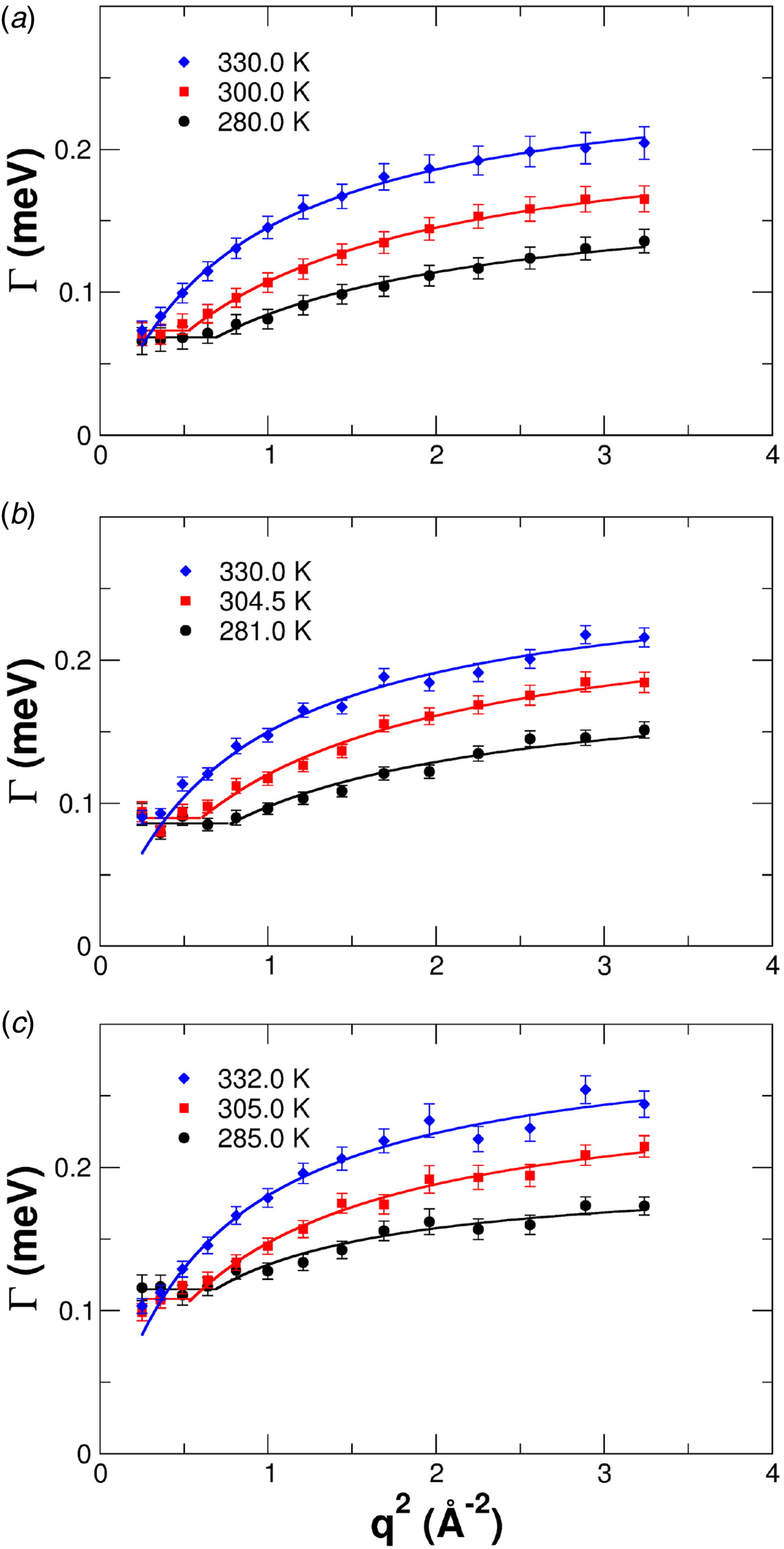
Further insight into the molecular basis for thermal adaptation is provided by MD simulations: Calligari et al. (Reference Calligari, Calandrini, Ollivier, Artero, Härtlein, Johnson and Kneller2015) combined MD simulations and QENS measurements of the protein Initiation Factor 6 (IF6) from Methanocaldococcus jannaschii (aIF6) at high temperature and pressure and its eukaryotic homolog from Saccharomyces cerevisiae under ambient conditions. Results obtained by MD were consistent with QENS data and showed once more that the two proteins share similar flexibility at the respective physiological temperatures, which can be fine-tuned by pressure (Calligari et al., Reference Calligari, Calandrini, Ollivier, Artero, Härtlein, Johnson and Kneller2015). The analysis of the scattering functions using a FBD model suggested that such a similarity is mainly due to entropic contributions. Furthermore, structure dependent analysis of the MD simulations showed that, in the extremophilic protein (aIF6), a suppression of the backbone flexibility with increasing pressure is compensated by an increased mobility of the amino acid side-chains, and that the most significant pressure- and temperature-induced flexibility changes occur in the bending regions between helices and β-strands. Finally, the differences between aIFS and its mesophilic (initiation factor 6 from S. cerevisiae (eIF6)) homolog were found to be due to the presence, in the latter protein, of a 20 amino acid tail, ensuring the necessary flexibility to eIF6 at ambient temperature (Calligari et al., Reference Calligari, Calandrini, Ollivier, Artero, Härtlein, Johnson and Kneller2015).
Summarizing, the reviewed results provide solid evidence for temperature adaptation of protein dynamics, ensuring comparable stability and function of proteins at their respective physiological temperatures (Tehei and Zaccai, Reference Tehei and Zaccai2007), and MD simulations help understanding the underlying molecular mechanisms.
Collective internal motions in proteins
As discussed in the Introduction, the protein exhibits a hierarchy of dynamics. So far, a picture of the local self-dynamics of atoms on timescales ranging from picoseconds to a few nanoseconds was provided. On a larger length scale, the motion of entire domains and subdomains takes place on timescales from nanoseconds to microseconds. Such movements can be directly observed at rather low protein concentrations by employing NSE spectroscopy combined with normal mode analysis of the protein crystal structure or a CG structural ensemble, as explained in detail in Callaway et al. (Reference Callaway, Farago and Bu2013); Richter (Reference Richter, Garcia Sakai, Alba-Simionesco and Chen2012); Monkenbusch and Richter (Reference Monkenbusch and Richter2007); Monkenbusch et al. (Reference Monkenbusch, Richter and Biehl2010); Callaway and Bu (Reference Callaway, Bu and Kelman2016, Reference Callaway and Bu2017); Stadler (Reference Stadler, Artmann, Artmann, Zhubanova and Digel2018); Biehl and Richter (Reference Biehl and Richter2014) and the modeling section ‘Modeling and analysis’.
To the best of our knowledge, the first NSE study regarding the domain motion of a protein was carried out in 1982 by Alpert et al. (Reference Alpert, Cser, Farago, Franek, Mezei and Ostanevich1982). The pig anti-Dnp-immunoglobulin (pIgG), an antibody protein, was modeled as two prolate ellipsoids of revolution connected at the end points of their longer axes (Fab arm) and an ellipsoid of revolution whose volume was equal to the volume of the Fab arm (Fc part) (Alpert et al., Reference Alpert, Cser, Farago, Franek, Mezei and Ostanevich1982). Samples at ~40 and ~80 mg ml−1 in the presence of ~200 mg ml−1 sucrose were measured at 14 °C. The comparison of the experimental scattering function with those expected for a rigid and two increasingly flexible pIgGs indicated that the molecule is subject to a rather large wobbling type motion of the Fab arms around the so-called hinge region within an angle of 50° (Alpert et al., Reference Alpert, Cser, Farago, Franek, Mezei and Ostanevich1982). A few years later, Alpert et al. (Reference Alpert, Cser, Faragó, Franěk, Mezei and Ostanevich1985) confirmed the result also in the absence of sucrose.
More recently, Stingaciu et al. (Reference Stingaciu, Ivanova, Ohl, Biehl and Richter2016) have studied IgG from human serum (hIgG) and observed that, on a timescale of 7 ns, hIgG fragments move with motional amplitudes of about 1 nm relative to each other. hIgG was measured at 29 mg ml−1 and 25 °C. Notably, the observed dynamics could be well described by a rather simple model neglecting the details of the complex interaction at the residue level in the linker region, which was instead modeled by an effective spring with a force constant of ~0.02 N m−1, while fragments undergo Brownian motion under a harmonic potential (Stingaciu et al., Reference Stingaciu, Ivanova, Ohl, Biehl and Richter2016).
In 2005, Bu and collaborators, measured coupled motion of domains separated by 70 Å of DNA polymerase I from Thermus aquaticus (Bu et al., Reference Bu, Biehl, Monkenbusch, Richter and Callaway2005). This motion is essential to coordinate nucleotide synthesis and cleavage during DNA synthesis and repair. In particular, at low concentration, the deviation of the effective diffusion coefficients from the diffusion coefficient measured by DLS was attributed to large-scale internal dynamics. These experimentally determined deviations were compared with those calculated assuming domain motions based on normal mode analysis. Thereby, it was shown that the motion of DNA polymerase I can be well approximated by a few normal modes of three coupled domains.
In a similar study, NSE revealed that catalytic activity of PGK is enabled by large domain fluctuations on the 50 ns timescale (Inoue et al., Reference Inoue, Biehl, Rosenkranz, Fitter, Monkenbusch, Radulescu, Farago and Richter2010). Small-angle scattering data revealed that the protein in solution has a more compact structure than that in a crystal, but the structural analysis indicated that the distance between residues taking part in the catalytic reaction would be too large if the protein were static. Correlation functions measured with NSE were characterized, above q ~ 0.08 Å−1, by a superposition of two decays. The slower of these was ascribed to the long-time translational and rotational diffusion, while the faster decay was attributed to internal dynamics. Normal mode data analysis indicated that domain movements facilitate a close encounter of the key residues in the active center to build the active configuration. Furthermore, the measurements showed that substrate binding induces faster domain motion, but with a simultaneous reduction of its amplitude. Hence, it was shown that the binding of a substrate leads to an increased rigidity of PGK. The results of this study were later compared with MD simulations, which confirmed that a significant component of the NSE signal arises from internal dynamics. The comparison also evidenced that the amplitudes of the motions derived by MD are smaller than those derived from the experimental analysis (Smolin et al., Reference Smolin, Biehl, Kneller, Richter and Smith2012).
The use of a normal mode approach was later justified by Hong et al. by analyzing neutron scattering data and performing MD simulations, as protein interdomain motion was shown to obey overdamped Langevin dynamics (Hong et al., Reference Hong, Smolin and Smith2014b). Moreover, the authors demonstrated that protein interdomain motion follows the principle of de Gennes narrowing, meaning that the wavevector dependence of the interdomain diffusion coefficient is inversely proportional to the interdomain structure factor. As noted by the authors (Hong et al., Reference Hong, Smolin and Smith2014b), this aspect can be understood as the domains moving slower with respect to each other when in favored spatial arrangements.
As an interesting example of joint use of complementary techniques, Hong et al. (Reference Hong, Sharp, Poblete, Biehl, Zamponi, Szekely, Appavou, Winkler, Nauss, Johs, Parks, Yi, Cheng, Liang, Ohl, Miller, Richter, Gompper and Smith2014a) investigated the structure and dynamics of the compact form of the multidomain protein mercuric ion reductase (MerA). MerA is a protein acting as an enzyme, which is central to the mercury resistance pathway found in many aerobic bacteria (Hong et al., Reference Hong, Sharp, Poblete, Biehl, Zamponi, Szekely, Appavou, Winkler, Nauss, Johs, Parks, Yi, Cheng, Liang, Ohl, Miller, Richter, Gompper and Smith2014a). By comparing the dynamics of the full length MerA and the bare catalytic core domain without linkers or NmerA domains, SANS indicated that MerA adopts a compact structure in solution with the NmerA domains in direct contact with the core (Hong et al., Reference Hong, Sharp, Poblete, Biehl, Zamponi, Szekely, Appavou, Winkler, Nauss, Johs, Parks, Yi, Cheng, Liang, Ohl, Miller, Richter, Gompper and Smith2014a). Moreover, NSE measurements and CG simulations indicated that the domain motion is of small amplitude and the linkers are relatively rigid (Hong et al., Reference Hong, Sharp, Poblete, Biehl, Zamponi, Szekely, Appavou, Winkler, Nauss, Johs, Parks, Yi, Cheng, Liang, Ohl, Miller, Richter, Gompper and Smith2014a). Finally, all-atom MD simulations indicated that the NmerA domain electrostatically interacts with the core, hence being in close contact with it, and undergoing a subdiffusive motion over its surface. Since it is believed that Hg2+ first binds to the Nmer domains and is then transferred to the catalytic site in the core, it was suggested by the authors that such an exploratory movement may facilitate the binding of Hg and a fast delivery to the core (Hong et al., Reference Hong, Sharp, Poblete, Biehl, Zamponi, Szekely, Appavou, Winkler, Nauss, Johs, Parks, Yi, Cheng, Liang, Ohl, Miller, Richter, Gompper and Smith2014a).
In order to understand the domain motion of complex proteins, selective deuteration can be employed. This was the case for NHERF1, a multidomain protein assembling protein complexes after being allosterically triggered by the binding of another protein, ezrin, 11 nm away from the active domains (Farago et al., Reference Farago, Li, Cornilescu, Callaway and Bu2010). NSE measurements of selectively deuterated NHERF1 highlighted the activation of interdomain collective dynamics on nanometer length-scales and on submicrosecond timescales after the formation of a complex with ezrin. The results demonstrated therefore that allosteric regulation can involve changes in long-range submicrosecond domain motions (Farago et al., Reference Farago, Li, Cornilescu, Callaway and Bu2010). Subsequent to this study, Callaway et al. (Reference Callaway, Matsui, Weiss, Stingaciu, Stanley, Heller and Bu2017) studied a phosphomimic mutation of NHERF1 at different NaCl concentrations, and hence ionic strengths, in order to investigate the role of electrostatics in allosteric regulation. The results showed that the phosphomimic mutation and the salt concentration alter the nanoscale dynamics and target-binding kinetics in the intrinsically disordered tail of NHERF1. The authors suggested that the electrostatic charges introduced by phosphomimic mutation NHERF1 cause the activation of specific internal dynamics, which can be reversed by increasing the salt concentration. Moreover, the kinetic association rate constant of the binding of the mutant to erzin was also found to correlate with the excited nanoscale dynamics. In fact, increased nanoscale dynamics was found to correspond to an improved binding ability (Callaway et al., Reference Callaway, Matsui, Weiss, Stingaciu, Stanley, Heller and Bu2017).
For additional details on the use of NSE for the study of the implications of protein dynamics changes on several timescales due to allosteric signaling, we refer the reader to Bu and Callaway (Reference Bu and Callaway2013) and Callaway and Bu (Reference Callaway and Bu2015). Additional neutron scattering studies regarding the role of the dynamics in allosteric regulation can be found in the ‘Relations of protein dynamics to structure: from globular to intrinsically disordered proteins’ section. Other techniques such as NMR, and fluorescence-based techniques, as well as MD simulations can also be employed to investigate this topic. Such studies have demonstrated that proteins respond to perturbations by redistributing their motions, even in the absence of detectable structural changes (Tzeng and Kalodimos, Reference Tzeng and Kalodimos2011). Moreover, there is also strong evidence for the crucial role of fluctuating conformational states and conformational entropy in the allosteric mechanism (Kern and Zuiderweg, Reference Kern and Zuiderweg2003; Tzeng and Kalodimos, Reference Tzeng and Kalodimos2011). Emerging evidence indicates furthermore that connecting, poorly structured regions of the polypeptide chain play an important role in allosteric regulation (Papaleo et al., Reference Papaleo, Saladino, Lambrughi, Lindorff-Larsen, Gervasio and Nussinov2016). For further reading on this topic, we refer the reader to Kern and Zuiderweg (Reference Kern and Zuiderweg2003); Tzeng and Kalodimos (Reference Tzeng and Kalodimos2011); Motlagh et al. (Reference Motlagh, Wrabl, Li and Hilser2014); Kornev and Taylor (Reference Kornev and Taylor2015); Papaleo et al. (Reference Papaleo, Saladino, Lambrughi, Lindorff-Larsen, Gervasio and Nussinov2016).
Recently, NSE has been successfully employed also to determine the internal dynamics of intrinsically disordered myelin basic protein (MBP) (Stadler et al., Reference Stadler, Stingaciu, Radulescu, Holderer, Monkenbusch, Biehl and Richter2014b; Stadler, Reference Stadler, Artmann, Artmann, Zhubanova and Digel2018) (further information on the dynamics in intrinsically disordered as well as denatured proteins and molten globules can be found in the ‘Comparison of internal protein dynamics in native, molten and denatured states’ and ‘Relations of protein dynamics to structure: from globular to intrinsically disordered proteins’ sections). First, small-angle scattering revealed that the protein compactness lies between that of a globular protein and that of a random coil polymer. Instead, the large contribution of the internal motions of the peptide chain to the overall diffusion measured by NSE indicated a high-structural flexibility with a relaxation rate of 8.4 ns. Collective stretching and bending motions, especially pronounced at the termini, were identified by normal mode analysis as the prominent contribution to the internal dynamics. Moreover, the data were found to be inconsistent with the Zimm model with internal friction derived from polymer theory. The inconsistency was interpreted by the authors as a result of the presence of a compact core and of a secondary structure content of 44%. Relaxations on correlation times of several nanoseconds to ~100 ns were observed in IDPs also with fast field cycling relaxation NMR (Parigi et al., Reference Parigi, Rezaei-Ghaleh, Giachetti, Becker, Fernandez, Blackledge, Griesinger, Zweckstetter and Luchinat2014) (probing proton relaxations, also at higher protein concentrations than in Stadler et al. (Reference Stadler, Stingaciu, Radulescu, Holderer, Monkenbusch, Biehl and Richter2014b)) and fluorescence spectroscopy (Mukhopadhyay et al., Reference Mukhopadhyay, Krishnan, Lemke, Lindquist and Deniz2007; Müller-Späth et al., Reference Müller-Späth, Soranno, Hirschfeld, Hofmann, Rüegger, Reymond, Nettels and Schuler2010; Liu et al., Reference Liu, Chia, Csizmok, Farber, Forman-Kay and Gradinaru2014) (dynamics of labeled residues), in the latter case depending also on the presence of salt. In addition to this, FRET studies detected conformational fluctuations on the millisecond or longer timescale in IDPs or in disordered domains (Huang et al., Reference Huang, Rajagopalan, Settanni, Marsh, Armoogum, Nicolaou, Bain, Lerner, Haas, Ying and Fersht2009; Lamboy et al., Reference Lamboy, Kim, Lee, Ha and Komives2011; Liu et al., Reference Liu, Chia, Csizmok, Farber, Forman-Kay and Gradinaru2014). Hence, the combination of neutron scattering and other techniques might be crucial also for a complete understanding of the internal collective dynamics of IDPs.
The NSE technique has the advantage to not only measure internal relaxations, but also explicitly relate such relaxations to the geometry of collective domain motions, providing essential information on mechanisms of protein function. NMR and FRET can complement the information on protein collective dynamics and its correlation times for a broader range of volume fractions. In fact, slow (nanosecond–millisecond) collective dynamics along the backbone of proteins could be observed also by NMR (Eisenmesser et al., Reference Eisenmesser, Bosco, Akke and Kern2002; Wolf-Watz et al., Reference Wolf-Watz, Thai, Henzler-Wildman, Hadjipavlou, Eisenmesser and Kern2004; Vögeli and Yao, Reference Vögeli and Yao2009; Fenwick et al., Reference Fenwick, Schwieters and Vögeli2016), usually at a residue level, although also the domain motion could be measured by combining SAXS, reorientational eigenmode dynamics analysis and NMR (Bernadó et al., Reference Bernadó, Modig, Grela, Svergun, Tchorzewski, Pons and Akke2010). For a better investigation of this type of motions in proteins, encouraging results were obtained with computational means with the recently developed essential collective dynamics method (Stepanova, Reference Stepanova2007; Barakat et al., Reference Barakat, Issack, Stepanova and Tuszynski2011; Santo et al., Reference Santo, Berjanskii, Wishart and Stepanova2011; Issack et al., Reference Issack, Berjanskii, Wishart and Stepanova2012; Dorosh et al., Reference Dorosh, Kharenko, Rajagopalan, Loewen and Stepanova2013; Stueker et al., Reference Stueker, Ortega, Goss and Stepanova2014), which was also successfully employed to interpret NMR data.
Particularly interesting for determining the protein domain motions in solution, on timescales of microseconds and milliseconds, is the recent development of a new methodology based on networks of distance distributions obtained from time-resolved single-molecule FRET (Hellenkamp et al., Reference Hellenkamp, Wortmann, Kandzia, Zacharias and Hugel2017). The approach was applied to the flexible multidomain heat-shock protein Hsp90. By combining the data from more than 100 pairs of FRET dyes across the entire Hsp90 dimer under various conditions in solution with MD simulations, Hellenkamp et al. (Reference Hellenkamp, Wortmann, Kandzia, Zacharias and Hugel2017) were able to show how Hsp90 interdomain dynamics changes depending on the protein state (open versus closed).
As mentioned in the Introduction, structural rearrangements of proteins during the transition from one state to another can be followed, in specific cases, by time-resolved X-ray scattering (see section ‘Scattering techniques’). Lately, also time-resolved neutron scattering profiting from deuterium labeling and contrast variation, and combined with fluorescence spectroscopy has been successfully employed to follow a coarse structural evolution of the protein complex PAN unfoldase PAN unfoldase (proteasome-activating nucleotidase in archaebacteria), on tens of seconds to minutes. More in detail, Ibrahim et al. (Reference Ibrahim, Martel, Moulin, Kim, Härtlein, Franzetti and Gabel2017) observed that, while unfolding its substrate, the PAN complex undergoes a transition from a relaxed to a contracted conformation, with a characteristic time of 315 ± 25 s, followed by a slower expansion to its initial state at the end of the reaction, with a characteristic time of 405 ± 30 s. The authors argued that the result supports a model in which these complexes unfold their substrates in a reversible power stroke mechanism involving several subunits (Ibrahim et al., Reference Ibrahim, Martel, Moulin, Kim, Härtlein, Franzetti and Gabel2017).
In summary, recent developments in different techniques enable the study of the concerted motion of protein domains on different, complementary timescales. Future studies combining these methods may considerably help understanding the hierarchy of domain dynamics and gathering more information on an in-depth understanding of these nanomachines.
Combination of neutron spectroscopy techniques: alcohol dehydrogenase
Both the internal and center-of-mass dynamics of ADH, a protein responsible for the interconversion between alcohol and ketones, were investigated with NSE, TOF and NBS, on a broad range of timescales (Biehl et al., Reference Biehl, Hoffmann, Monkenbusch, Falus, Prévost, Merkel and Richter2008; Stadler et al., Reference Stadler, Monkenbusch, Biehl, Richter and Ollivier2013a; Monkenbusch et al., Reference Monkenbusch, Stadler, Biehl, Ollivier, Zamponi and Richter2015).
Biehl et al. (Reference Biehl, Hoffmann, Monkenbusch, Falus, Prévost, Merkel and Richter2008) determined the main domain motions of ADH by employing NSE. The difference  ${\rm \Delta} D_{{\rm eff}}^0 $ between the measured diffusion coefficient $D_{{\rm eff}}^0 $ and that calculated accounting for translation and rotational diffusion is shown in Fig. 17a as a function of q. Such a difference is due to slow collective internal dynamics. The analysis of the q-dependence of ${\rm \Delta} D_{{\rm eff}}^0 $ and its comparison with the diffusion coefficients calculated based on normal mode analysis (Fig. 17b) revealed the occurrence of two main domain motions shown in Fig. 17c, one of which corresponds to the opening and closing of a cleft in the protein structure, between the binding and the catalytic domains (Biehl et al., Reference Biehl, Hoffmann, Monkenbusch, Falus, Prévost, Merkel and Richter2008). This motion enables the binding and release of the cofactor required for the conversion of ethanol to acetaldehyde. Moreover, the analysis indicated that, when the cofactor is bound, the mode related to the opening and closing of the cleft is reduced, denoting a stiffening of the concerned domains.
(a) Difference of the corrected diffusion coefficients  $D_{eff}^{0}(q)$ and the calculated translational or rotational diffusion coefficient. (b) Diffusion form factor of the normal modes 7 and 11 for the protein configuration with and without the cofactor. (c) Top – Motional pattern of mode 7: without cofactor the exterior domain (catalytic domain) tilts outward and opens the cleft. The inner domain with connection points between the monomers remains stiff. Bottom: Motional pattern of mode 11: with and without the bound cofactor the monomers within a dimer exhibit torsional motion around the long dimer axis (in the image plane), which is more pronounced with the cofactor. Figure reproduced with permission from (Biehl et al., Reference Biehl, Hoffmann, Monkenbusch, Falus, Prévost, Merkel and Richter2008). Copyright American Physical Society.
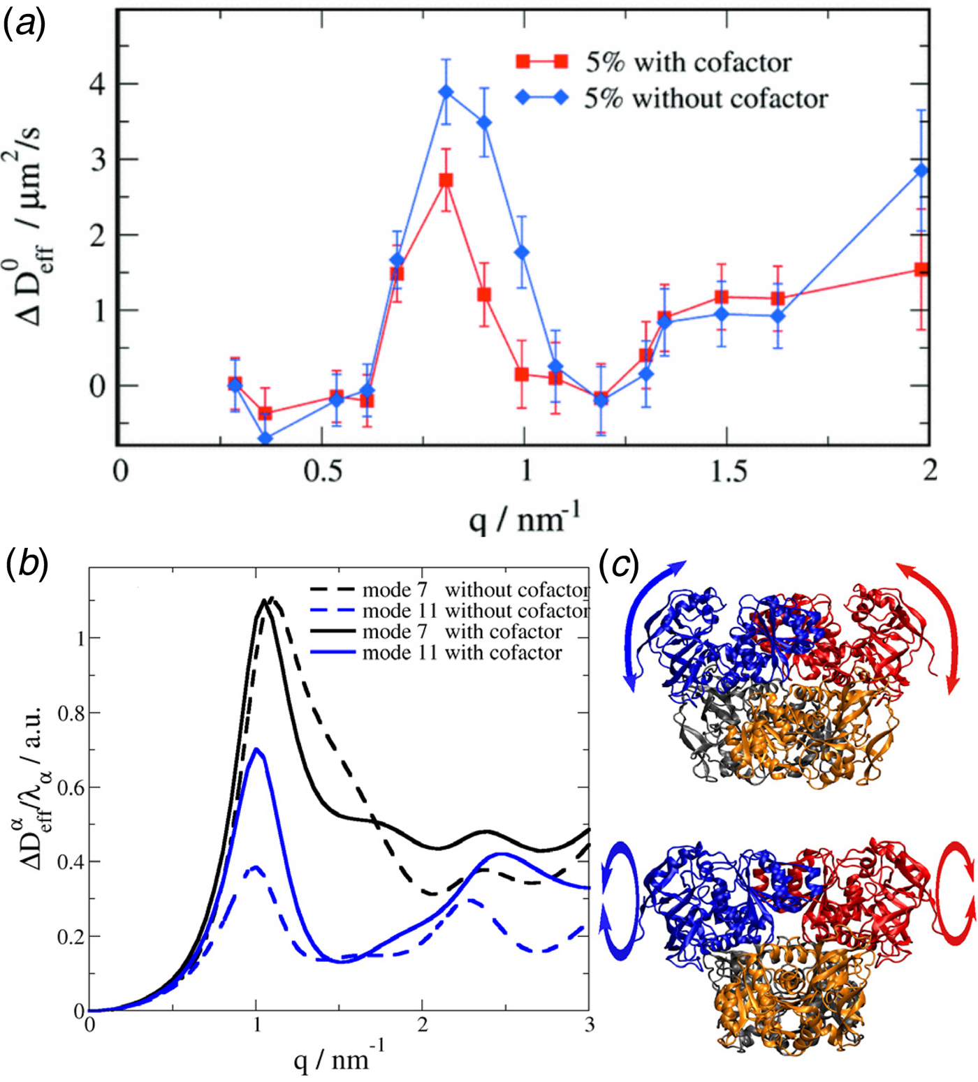
The diffusion coefficient and the slow internal relaxation obtained with NSE were fixed in a global fit of TOF and NBS data (Monkenbusch et al., Reference Monkenbusch, Stadler, Biehl, Ollivier, Zamponi and Richter2015). The fitted model considered atoms to belong to one of three classes of motions occurring on top of rotation and translation of the entire protein: (i) atoms immobile with respect to the protein as a rigid body; (ii) atoms undergoing large scale domain motions and (iii) atoms participating in fast localized motions. In addition, atoms belonging to each of the three classes were free to distribute over 10 concentric shells comprising the protein. Approximately 34–37% of the atoms were found to undergo fast diffusive motions with the diffusion coefficient D s ranging between 65 and 78 Å2 ns−1 in a confined volume with an effective radius of 7.1–7.5 Å, depending on whether class (ii) was taken into account or not. It was noted by the authors that the results are consistent with a more simple analysis combining NSE and TOF, but not NBS data on ADH, yielding a fraction of mobile atoms around 35%, and a radius R ~ 8 Å (Stadler et al., Reference Stadler, Monkenbusch, Biehl, Richter and Ollivier2013a), and with the results in Grimaldo et al. (Reference Grimaldo, Roosen-Runge, Zhang, Seydel and Schreiber2014), where R ~ 6.7 Å. A further outcome of the model is that most H-atoms undergoing fast movements seemed to be close to the surface, while those being immobile seem to be located mainly in the center. It was therefore hypothesized that the fast motions result from direct interaction of amino acids at the surface with the surrounding water.
In conclusion, the analysis of NSE, TOF and NBS data proposed by Monkenbusch et al. (Reference Monkenbusch, Stadler, Biehl, Ollivier, Zamponi and Richter2015) to model the dynamics of ADH suggested the presence of three distinct dynamical processes: one due to the translation and rotation of the protein, the second, occurring on tens of nanoseconds, due to domain motion and the third, occurring on hundreds of picoseconds, related to fast localized motions at the amino acid level. Moreover, the model suggested that the third component is mainly arising from motions of amino acids in the outer shells, close to the solvent, whereas those in the inner parts appeared immobile.
In vivo neutron spectroscopy
In addition to the EINS measurements of living bacteria and RBCs presented in the ‘Adaptation of proteins to ambient and extreme temperatures’ section, other neutron spectroscopy studies have been performed in living E. coli and human RBCs, exploiting instruments accessing different timescales.
The first attempts to measure Hb diffusion at rather high concentrations and in RBCs, as well as the dynamics of an entire bromegrass mosaic virus with neutron scattering date back, to the best of our knowledge, to 1980, when Alpert (Reference Alpert1980) was testing the applicability of NSE to biological systems. In this pioneering experiment, Alpert was able to measure the diffusion of Hb at 295 K and c p = 120 and 180 mg ml−1, obtaining 3.7 and 3.0 Å2 ns−1, respectively, hence significantly lower than the dilute limit diffusion coefficient D 0 ≃ 5.6 Å2 ns−1 in D2O (Alpert, Reference Alpert1980). Furthermore, a much lower relaxation rate, also with a different q-dependence, was observed in the RBCs compared with the Hb solutions. No significant dynamics could be observed in the bromegrass mosaic virus, likely because the signal was too weak and the dynamics too slow for the spectrometers at that time.
Later, Hb diffusion in RBCs was studied again using NSE spectroscopy by Doster and Longeville (Reference Doster and Longeville2007). The measured time and wavevector behavior suggested the crossover of self- and collective diffusion in the accessible time and q-range. The data revealed feature characteristics of hydrodynamic interactions between the proteins, and the diffusion coefficients (in RBC containing H2O, at 20 °C D = 1.1 Å2 ns−1) agreed quantitatively with long-time self-diffusion coefficients from the theory of hard-sphere suspensions, after adjusting the volume fraction of Hb by including the volume of the hydration layer to the dry protein volume. The results suggested therefore the applicability of concepts of colloid physics to proteins. It was concluded from these results that hydrodynamic interactions dominate long-range molecular transport at physiological concentrations.
In a recent study by Longeville and Stingaciu (Reference Longeville and Stingaciu2017) the diffusion of Hb in RBCs was again measured with NSE and quantitative agreement was found with that in an aqueous solution of Hb at a concentration similar to that within the cells. Moreover, diffusion was reported to be Brownian, up to the accessed timescale (~50 to ~100 ns) and concentrations (~330 mg ml−1). Remarkably, using a rather simple model for the kinetics of oxygen uptake by Hb in the lungs, the authors found that the diffusion of Hb facilitates the oxygen capture of the RBCs, and that the Hb concentration in the RBCs corresponds to an optimum of oxygen capture for an individual under physical activity (Longeville and Stingaciu, Reference Longeville and Stingaciu2017).
An earlier study on Hb dynamics in RBC was performed with two backscattering spectrometers with different energy resolutions (Stadler et al., Reference Stadler, Van Eijck, Demmel and Artmann2010). The scattering function of both spectrometers was modeled with two dynamical contributions, one arising from the protein global diffusion (translation and rotation of the whole protein), the other due to internal motions. Different apparent global diffusion coefficients were obtained from each instrument. The translational diffusion coefficient was extracted from the apparent coefficient, and compared with the values expected from the theory of colloidal suspensions. Similar to Doster and Longeville (Reference Doster and Longeville2007), Stadler et al. (Reference Stadler, Van Eijck, Demmel and Artmann2010) added the volume of the hydration layer to that of the bare protein in calculating the volume fraction. After this correction, the two translational diffusion coefficients were found to agree quantitatively with the expected short- and long-time self-diffusion coefficients. Regarding the internal Hb dynamics, the faster contribution was attributed to localized jump-diffusion with D jump ~ 300 Å2 ns−1 and τ 0 ~ 4 ps at 20 °C. The slow internal contribution was rather q-independent and its correlation time at 27 °C was ~100 ps. While the fast internal dynamics was higher than in fully hydrated Hb powder, the slow component was found to be rather similar to that of fully hydrated protein powders, solutions and E. coli cells reported in other studies (Stadler et al., Reference Stadler, Van Eijck, Demmel and Artmann2010).
Jasnin et al. (Reference Jasnin, Moulin, Härtlein, Zaccai and Tehei2008a) carried out measurements of E. coli on three different spectrometers providing access to dynamics on a wide range of timescales. Several types of motions were identified and associated with contributions from diverse dynamical classes. Three types of motions were associated with internal processes. A fast relaxation was attributed to confined jump-diffusion motions with correlation times of 4.7 and 3.6 ps at 280 and 300 K, respectively. A slower process characterized by a q-independent quasi-elastic broadening was assigned to rotational motions occurring on characteristic times of ~40 ps. It was noted by the authors that this process may arise from stochastic reorientations of large molecular subunits, such as polypeptide side-chains, fatty acid chains or other molecular subunits, as well as rotational motions of smaller groups such as protons in methyl groups. The slowest dynamical contribution associated with internal dynamics was also characterized by a q-independent quasi-elastic broadening and was therefore ascribed to rotational motions, with correlation times of ~94 and 90 ps at 284 and 303 K, respectively. The authors interpreted this contribution as due, for example, to librations of buried groups, relative displacements of globular domains, sugar conformational changes or RNA global bending. A comparison of the results of this study with those in hydrated powders led Jasnin and co-workers to the conclusion that the cellular environment induces a significant enhancement of internal dynamics. Instead, the in vivo dynamics appeared limited compared with that measured in solutions. It was therefore inferred that macromolecular interactions and confinement typical of physiological environments is not mimicked accurately by protein solutions, and it was suggested that intracellular complexity may participate in functional dynamics necessary for biological activity (Jasnin et al., Reference Jasnin, Moulin, Härtlein, Zaccai and Tehei2008a). Finally, an even slower dynamical contribution showing typical features of jump-diffusion was attributed to the average macromolecular self-diffusion with diffusion coefficients 0.85 ± 0.15 Å2 ns−1 = 0.85 ± 0.15 × 10⁻⁷cm2 s−1 and 1.06 ± 0.11 Å2 ns−1 at 284 and 303 K, consistent with the measurements of self-diffusion in RBCs (Doster and Longeville, Reference Doster and Longeville2007). The respective residence times were τ = 0.97 ± 0.08 and τ = 0.59 ± 0.04 ns.
Further in vivo studies were performed on extremophile bacteria in the context of the adaptation to extreme temperatures and pressures (Tehei et al., Reference Tehei, Franzetti, Madern, Ginzburg, Ginzburg, Giudici-Orticoni, Bruschi and Zaccai2004; Tehei and Zaccai, Reference Tehei and Zaccai2005; Martinez et al., Reference Martinez, Michoud, Cario, Ollivier, Franzetti, Jebbar, Oger and Peters2016), see sections ‘Internal dynamics of proteins at high pressure’ and ‘Adaptation of proteins to ambient and extreme temperatures’. The solvent isotope effect on in vivo protein dynamics was studied in E. coli (Jasnin et al., Reference Jasnin, Tehei, Moulin, Härtlein and Zaccai2008b), see section ‘From powder to solution: influence of solution conditions on protein dynamics’.
Recently, even multicellular living organisms, namely planarian flatworms, have been studied by QENS (Mamontov, Reference Mamontov2018). Mamontov (Reference Mamontov2018) found two remarkably well defined pico- to nano-second dynamical contributions to the scattering function, one of which was attributed to water diffusion and the other to the dynamics of the other cellular constituents. Since the quasielastic broadenings γ had no obvious q 2-dependence, they were fitted both with a jump-diffusion model and a Fickian diffusion model. In both cases, the diffusion coefficients in a temperature range of 284.5–304.1 K were not increasing according to the Stokes–Einstein coefficient, but rather decoupled from the solvent diffusivity, as expected instead for the lateral diffusion of lipids in membranes. Moreover, the author noted, independent of the model, the diffusion coefficients seemed to exhibit systematically higher values above 298 K compared with the lower measurement temperatures, reasonably consistent with the well-known phase transition in lipid assemblies around that temperature (Mamontov, Reference Mamontov2018). Hence, it was suggested by the author that the measured component was at least mainly due to lipid diffusion. Finally, Mamontov speculated that the fact that temperatures higher than 294–296 K may eventually damage planarians may be related to the possible increase in the diffusivity of cell constituent above 298 K and possibly a diminished ability to maintain tightly the diffusivity in their cell constituents at elevated temperatures (Mamontov, Reference Mamontov2018).
While the studies so far monitored the dynamics of all cellular components, Anunciado et al. reported a study on the global and internal dynamics of only a particular protein in a living bacterial cell (Anunciado et al., Reference Anunciado, Nyugen, Hurst, Doktycz, Urban, Langan, Mamontov and O'Neill2017). Using overexpression of protonated GroEL protein in a deuterated E. coli, the global diffusion was found to be slowed down by a factor of 4 compared with dilute buffer conditions. Furthermore, internal motions were found to be slowed down by roughly a factor of 2 from ~ 39 ps under buffer conditions to ~ 65 ps, while their confinement geometry remained similar with a confinement radius of about 1.3 Å (Anunciado et al., Reference Anunciado, Nyugen, Hurst, Doktycz, Urban, Langan, Mamontov and O'Neill2017).
Other techniques such as NMR and fluorescence spectroscopy are in principle suitable to study specific protein dynamics in living cells. NMR has the potential to detect the dynamics of a selected type of labeled protein. Such measurements are still a major challenge mainly due to the limited signal produced by low concentrated proteins and their interactions with the crowded cellular environment (Hänsel et al., Reference Hänsel, Luh, Corbeski, Trantirek and Doetsch2014). So far, only a few proteins have yielded sufficiently good NMR spectra in this context (Freedberg and Selenko, Reference Freedberg and Selenko2014; Hänsel et al., Reference Hänsel, Luh, Corbeski, Trantirek and Doetsch2014). Fluorescence techniques such as FRAP and FCS provide further complementary information on diffusion and binding of labeled macromolecules in living cells down to the microsecond timescale, with high-spatial resolution (Lippincott-Schwartz et al., Reference Lippincott-Schwartz, Snapp and Kenworthy2001; Diekmann and Hoischen, Reference Diekmann and Hoischen2014; Wachsmuth, Reference Wachsmuth2014). While several in vivo studies on diffusion as observed by FCS have reported a subdiffusive, anomalous behavior, other observations were consistent with normal Brownian diffusion (Höfling and Franosch, Reference Höfling and Franosch2013), and even unobstructed Brownian diffusion was reported for GFP in the cell cytoplasm on the 1 µs timescale, and explained as a consequence of the presence of rather immobile structures (the endoplasmic reticulum sheets, mitochondria, vesicles, Golgi apparatus, etc.), rather than of freely diffusing macro-molecules (Di Rienzo et al., Reference Di Rienzo, Piazza, Gratton, Beltram and Cardarelli2014). The question of the generality of anomalous diffusion is a topic of current discussion, and whether or not it occurs as well as how strong the deviation is from normal diffusion may depend on the moment in time of the cell life cycle (Selhuber-Unkel et al., Reference Selhuber-Unkel, Yde, Berg-Sørensen and Oddershede2009) (related to changes in the cellular environment) and on the position in the cell, the nucleus seemingly leading to the largest anomalies (Wachsmuth et al., Reference Wachsmuth, Waldeck and Langowski2000; Höfling and Franosch, Reference Höfling and Franosch2013). Also, whether the obstacles are mobile or immobile and the size of the probe seems to play a crucial role in the appearance of anomalous behaviors, as demonstrated by experiments and simulations (Berry and Chaté, Reference Berry and Chaté2014; Sentjabrskaja et al., Reference Sentjabrskaja, Zaccarelli, De Michele, Sciortino, Tartaglia, Voigtmann, Egelhaaf and Laurati2016). For further reading on the question of anomalous diffusion in biological cells, we refer the reader to Höfling and Franosch (Reference Höfling and Franosch2013) and Cardarelli and Gratton (Reference Cardarelli, Gratton and Jameson2016). Usually, fluorescence studies reported diffusion coefficients 3–10 times smaller than in dilute aqueous solutions (Luby-Phelps et al., Reference Luby-Phelps, Castle, Taylor and Lanni1987; Arrio-Dupont et al., Reference Arrio-Dupont, Cribier, Foucault, Devaux and d'Albis1996; Elowitz et al., Reference Elowitz, Surette, Wolf, Stock and Leibler1999; Schwille et al., Reference Schwille, Haupts, Maiti and Webb1999; Arrio-Dupont et al., Reference Arrio-Dupont, Foucault, Vacher, Devaux and Cribier2000; Wachsmuth et al., Reference Wachsmuth, Waldeck and Langowski2000; Lippincott-Schwartz et al., Reference Lippincott-Schwartz, Snapp and Kenworthy2001; Dauty and Verkman, Reference Dauty and Verkman2005), although also values smaller by a factor 104 were reported for large proteins in muscle cells (Arrio-Dupont et al., Reference Arrio-Dupont, Cribier, Foucault, Devaux and d'Albis1996, Reference Arrio-Dupont, Foucault, Vacher, Devaux and Cribier2000). Frequently, an increase of this factor with rising size of the probe was reported and often explained by the hindrance due to filamentous networks permeating the cells (Höfling and Franosch, Reference Höfling and Franosch2013), such as the cytoskeleton, with typical mesh sizes of 20–250 nm (Charras et al., Reference Charras, Hu, Coughlin and Mitchison2006; Morone et al., Reference Morone, Fujiwara, Murase, Kasai, Ike, Yuasa, Usukura and Kusumi2006; Salbreux et al., Reference Salbreux, Charras and Paluch2012) becoming particularly relevant at the long time probed by fluorescence spectroscopy.
The cellular environment and its implications for the macromolecular dynamics have been subject of an increasing number of computational studies in the past decade (Feig et al., Reference Feig, Yu, Wang, Nawrocki and Sugita2017). Generally, such studies achieved a rather good agreement with experimental observations and gave valuable information on the heterogeneity of the internal dynamics of biomacromolecules under crowded conditions (Feig et al., Reference Feig, Yu, Wang, Nawrocki and Sugita2017). Regarding the translational diffusion in the cellular environment simulations provided further insight into the crucial role of hydrodynamic interactions in slowing down the diffusion of highly concentrated spherical colloidal particles with a size distribution inspired from that of the components of E. coli cytoplasm (Ando and Skolnick, Reference Ando and Skolnick2010), as well as into the importance of the intrinsic polydispersity of bacterial cytoplasm in suppressing the occurrence of glassy dynamics at high concentrations (Hwang et al., Reference Hwang, Kim and Sung2016).
In summary, evidence for a substantially decreased diffusion of proteins in living cells compared with dilute solutions has been gathered by several complementary techniques, covering timescales from nanoseconds to hundreds of seconds. In some cases, especially on shorter timescales, concepts of colloid physics were applied to understand the diffusive properties of the macromolecules. On longer timescales, anomalous diffusion was often, but not always, observed by FCS. Its occurrence seems ultimately related to the characteristics of the local environment, and, although a complete physical picture is still missing, some studies indicate that it may be influenced by the presence of rather immobile structure versus freely diffusing macromolecules and the size of the probe relative to typical lengths characterizing the structure.
In vitro studies on the effect of macromolecular crowding on protein dynamics
One of the strengths of high-resolution neutron scattering spectroscopy is the possibility to investigate the dynamics of proteins up to very high solution concentrations. The study of proteins at high concentrations is motivated by the fact that the environment in which most proteins are found in living cells is crowded, i.e. it is filled with several types of macromolecules at volume fractions between 20 and 30% (Ellis, Reference Ellis2001). In the following, we review the results of in vitro neutron experiments under such conditions (see section ‘In vivo neutron spectroscopy’ for measurements of dynamics in vivo).
Global diffusion
The most obvious effect of crowding is on global translational and rotational diffusion of entire proteins. Several studies were carried out in order to understand and quantify such an effect. Mb dynamics at high concentrations was investigated using NSE by Longeville and co-workers (Longeville et al., Reference Longeville, Doster, Diehl, Gaehler, Petry, Mezei, Pappas and Gutberlet2003a, Reference Longeville, Doster and Kali2003b) and by Le Coeur and Longeville (Reference Le Coeur and Longeville2008). At q ~ 0.3 Å−1, collective diffusion approaches the self-diffusion (cf. section ‘Diffusion of the entire protein’). The self-diffusion coefficient D s was found to decrease with concentration (Longeville et al., Reference Longeville, Doster and Kali2003b). Compared with the dilute limit, D s for 32 mM (~530 mg ml−1) Mb was reduced by a factor of 15 (Longeville et al., Reference Longeville, Doster, Diehl, Gaehler, Petry, Mezei, Pappas and Gutberlet2003a). After the volume of one hydration layer on the surface was added to that of the bare protein to calculate the volume fraction – as done by Doster and Longeville (Reference Doster and Longeville2007) for Hb in RBCs – the measured diffusion coefficients were found to agree remarkably well with the long-time self-diffusion coefficient predicted by the theory of colloidal hard spheres (Le Coeur and Longeville, Reference Le Coeur and Longeville2008). The same was observed also in a subsequent NSE experiment by Longeville and Stingaciu (Reference Longeville and Stingaciu2017). The collective diffusion at low q, instead, was shown to increase with concentration as a result of increasing direct interactions (Longeville et al., Reference Longeville, Doster, Diehl, Gaehler, Petry, Mezei, Pappas and Gutberlet2003a). In a similar NSE experiment, Wood et al. (Reference Wood, Caronna, Fouquet, Haussler, Natali, Ollivier, Orecchini, Plazanet and Zaccai2008) reported a decrease of the diffusion of ribonuclease A with increasing concentration.
In an attempt to measure also the short-time limit of the diffusion coefficient by NSE, Hb was measured at 350 mg ml−1 in H2O (Le Coeur and Longeville, Reference Le Coeur and Longeville2008). Two relaxations were observed at 1 Å−1, one of which was attributed to water diffusion. The second component with relaxation time τ = 67 ± 15 ps was too fast due to short-time diffusion and it was not possible to determine the related process.
Later, Lal et al. (Reference Lal, Fouquet, Maccarini and Makowski2010) investigated Hb and Mb at two protein concentrations (20 and 150 mg ml−1) and two temperatures (15 and 37 °C) employing NSE at rather high scattering vectors 0.1 Å−1 < q <1 Å−1 (small length scales). For q>0.26 Å−1, the NSE intermediate scattering function was well fitted with a single exponential decay exp ( − t/τ). The relaxation times τ of Hb and Mb as a function of q showed marked differences. While for Mb the q-dependence could be interpreted in terms of a relatively rigid, freely diffusing quasi-spherical particle, for Hb an increase of τ with q was attributed to both additional rotational diffusion and internal modes (Lal et al., Reference Lal, Fouquet, Maccarini and Makowski2010). For q >0.26 Å−1, where the signal was interpreted in terms of self-correlations due to the predominant contribution of incoherent scattering, the intermediate scattering function could not be fitted by single-exponential function, and a KWW function (Williams and Watts, Reference Williams and Watts1970) (see section ‘Localized internal dynamics’) was used instead. After extracting the MSD $\langle r^2 (t)\rangle $ for q > 0.26 Å−1 as a function of time from several picoseconds to a few nanoseconds, found that <r 2(t)> ~ t β, with β = 0.4 ± 0.03, indicating subdiffusive motion, and that, for all timescales measured, <r 2(t)> was greater than expected if proteins were rigid. Hence, the authors concluded that the additional dynamics must be due to internal motion. In addition, MSDs at 150 mg ml−1 were found to be slower than those at 20 mg ml−1, consistent with several other studies (cf. section ‘In vitro studies on the effect of macromolecular crowding on protein dynamics’). The KWW characteristic time τ KWW ~ q −2/β, i.e. with a steeper q-dependence than for simple diffusion. Such a behavior, noted by the authors, is similar to that observed in polymer systems and in simulations of the dynamics of protein backbone atoms (Lal et al., Reference Lal, Fouquet, Maccarini and Makowski2010). It was suggested by Lal and co-workers that the observation of a stretched-exponential decay at high q-values results from the superposition of processes on at least three time regimes: an essentially harmonically, constrained fast motion at short times, concerted domain motions at intermediate times, and whole-body diffusion at longer times (Lal et al., Reference Lal, Fouquet, Maccarini and Makowski2010).
Mb diffusion up to a volume fraction of 40% was measured also by using NBS spectrometers (Busch et al., Reference Busch, Doster, Longeville, Sakai, Unruh and Sokol2006). Two components of the scattering function were identified: the slow relaxation was attributed to translational diffusion (neglecting rotational diffusion), whereas the fast process was assigned to internal dynamics. The narrow quasi-elastic broadening was found to follow a q-behavior typical of subdiffusive processes. The data were fitted with the jump-diffusion model by Singwi and Sjölander (see section ‘Localized internal dynamics’), and the diffusion coefficients were found to decrease with increasing protein concentration, whereas the residence times increased.
Similar results were observed in solutions of ferritin, a complex consisting of protein units responsible for iron storage (Häußler, Reference Häußler2008). At low concentrations and high-ionic strength, the diffusion measured by NSE approaches the dilute limit. Increasing the concentration, as expected, slows down the diffusion. The study examined also solutions with low-salt content. In these samples, a structure factor peak appeared as a consequence of the ordering of the ferritin molecules. In the vicinity of the peak, only an approximate analysis was possible, because the q-averaged intermediate scattering function is affected by the slope of the structure factor. Nevertheless, the data indicated that in low-salt samples both direct electrostatic and indirect interactions influence the ferritin dynamics, especially close to the structure factor. These results essentially confirmed those by Häussler and Farago on apoferritin (ferritin without the iron core) suggesting that, at the structure factor peak, dynamics is slowed down by strong spatial correlations, while at lower scattering vectors (larger length scales), dynamics is hindered by hydrodynamic interactions (Häußler and Farago, Reference Häußler and Farago2003).
Recently, Gupta et al. (Reference Gupta, Biehl, Sill, Allgaier, Sharp, Ohl and Richter2016) have mimicked a crowded environment by dispersing model globular proteins such as α-lactalbumin and Hb, in aqueous solution of poly(ethylene oxide). By employing NSE and SANS, the corresponding protein dynamics in semidilute polymer solution was measured. The authors could describe protein dynamics in such a crowded environment analogous to the diffusion under a periodic potential. A fast dynamic process was attributed to diffusion inside a trap built by the polymer mesh whereas a slower process was interpreted in terms of long time diffusion on macroscopic length scales also observed by other techniques. Moreover, for higher concentrated polymer solutions, the onset of fractional diffusion was observed (Gupta et al., Reference Gupta, Biehl, Sill, Allgaier, Sharp, Ohl and Richter2016). Previously, it was observed by NMR that the effect of crowding by a polymer mesh on long-time diffusion is qualitatively different from that of crowding by proteins (Wang et al., Reference Wang, Li and Pielak2010). Instead, the dynamics observed by Gupta et al. (Reference Gupta, Biehl, Sill, Allgaier, Sharp, Ohl and Richter2016) is likely rather analogous to that of a protein in nucleic acids such as DNA chains, or similarly trapping local environments within the cytoplasm. In fact, the long-time translational diffusion of GFP and BSA as a function of the concentration of DNA as investigated by FRAP (Wattenbarger et al., Reference Wattenbarger, Bloomfield, Bu and Russo1992; Busch et al., Reference Busch, Kim and Bloomfield2000) and NMR (Wang et al., Reference Wang, Li and Pielak2010) is qualitatively more similar to that observed in the presence of rather large synthetic polymers (Furukawa et al., Reference Furukawa, Arauz-Lara and Ware1991; Wang et al., Reference Wang, Li and Pielak2010) than in the presence of freely diffusing proteins or cell lysate (Wang et al., Reference Wang, Li and Pielak2010). Different dynamical behaviors might be related to the strand-like, meshing and more trapping nature of the DNA and polymers compared with the proteins.
The effect of crowding and the presence of NaCl on the diffusion of BSA was investigated using both NBS and NSE (Roosen-Runge et al., Reference Roosen-Runge, Hennig, Seydel, Zhang, Skoda, Zorn, Jacobs, Maccarini, Fouquet and Schreiber2010; Reference Roosen-Runge, Hennig, Zhang, Jacobs, Sztucki, Schober, Seydel and Schreiber2011). A crowding-induced decrease of the apparent self-diffusion coefficient D app was observed with both techniques. The addition of NaCl was found to affect the diffusion only at low protein concentrations (Roosen-Runge et al., Reference Roosen-Runge, Hennig, Seydel, Zhang, Skoda, Zorn, Jacobs, Maccarini, Fouquet and Schreiber2010). Later, Heinen et al. (Reference Heinen, Zanini, Roosen-Runge, Fedunova, Zhang, Hennig, Seydel, Schweins, Sztucki, Antalik, Schreiber and Nägele2012) investigated the static and dynamic properties of aqueous BSA solutions employing DLS, SLS, SAXS and rheometry integrated with analytical colloid theory. In the absence of salt, the long-time collective diffusion coefficients were found to rapidly increase from D 0 ~ 5 Å2 ns−1= 50 m2 s−1 in the dilute limit, to roughly 25 Å2 ns−1 at 10 mg ml−1 and then linearly decrease to ~25 Å2 ns−1 at 120 mg ml−1. The increase, observed in the collective diffusion measured by DLS but not in the self-diffusion measured in another study by NBS (Roosen-Runge et al., Reference Roosen-Runge, Hennig, Zhang, Jacobs, Sztucki, Schober, Seydel and Schreiber2011), is due to the repulsive nature of the interactions between BSA molecules, and was less and less marked with increasing screening induced by the addition of NaCl. Notably, while intentionally keeping the modeling rather simple, the measured static and dynamic features of the system were captured with semi-quantitative accuracy by such a colloid physics approach. Roosen-Runge et al. (Reference Roosen-Runge, Hennig, Zhang, Jacobs, Sztucki, Schober, Seydel and Schreiber2011) established an analytical framework for separating the rotational D r and the translational D t contributions to the experimentally determined D app, requiring knowledge of D r (see also section ‘Diffusion of the entire protein’). Using the short-time limit of D r from the theory of colloids, D t could be extracted from the data at 280 and 300 K and its value as a function of the protein volume fraction φ, calculated with the hydrodynamic radius R h rather than the bare protein radius R p, was found to agree quantitatively with the corresponding theoretical short-time translational diffusion coefficients, as shown in Fig. 18. Therefore, hydrodynamic interactions arising from self-crowding at physiological volume fractions (between 20 and 30%) were shown to slow down short-time self-diffusion by a factor 5 compared with the dilute limit (Roosen-Runge et al., Reference Roosen-Runge, Hennig, Zhang, Jacobs, Sztucki, Schober, Seydel and Schreiber2011). A slowing down generally on the same order of magnitude or more pronounced was observed on longer timescales by fluorescence spectroscopy in vitro (Höfling and Franosch, Reference Höfling and Franosch2013), as well as in vivo, as reported in the previous section.
Translational self-diffusion coefficients D t normalized by the dilute limit diffusion coefficient D t(0) (circles) for two different temperatures (red and purple circles denote 280 and 300 K, respectively) after separation of the rotational contributions. The purple line superimposed on the data is a guide to the eye obtained from a polynomial fit indicating the temperature-independent master-curve. The top and bottom dashed purple lines indicate the upper and lower 96% prediction bounds, respectively. The blue lines denote the colloidal short-time self-diffusion for hard spheres (light blue, solid) and charged spheres (dark blue, dashed). The inset in the top right corner illustrates the flow field (light blue stream line plot) generated by the movement of three spheres (velocities are denoted by blue arrows) and therefore experiencing hydrodynamic forces (pink arrows). Figure reproduced with permission from Roosen-Runge et al. (Reference Roosen-Runge, Hennig, Zhang, Jacobs, Sztucki, Schober, Seydel and Schreiber2011). Copyright National Academy of Sciences of the United States of America.
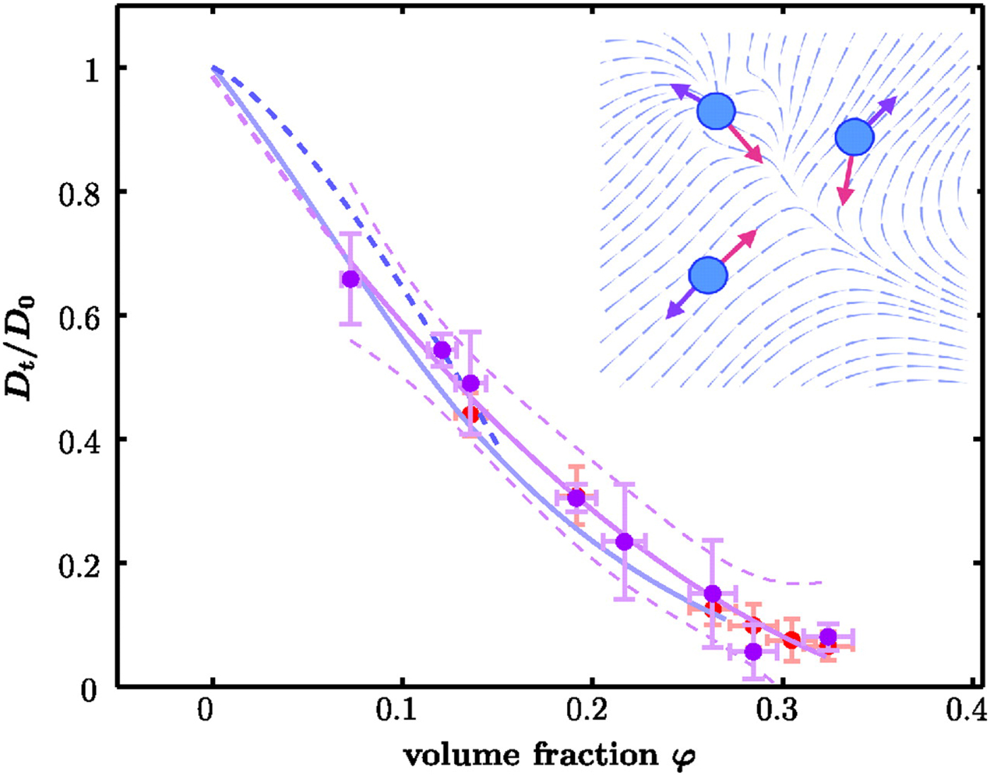
In a subsequent NBS study, Grimaldo et al. (Reference Grimaldo, Roosen-Runge, Zhang, Seydel and Schreiber2014) measured the apparent self-diffusion of the distinctly non-spherical Y-shaped γ-globulins in D2O as a function of φ. As for BSA, the short-time self-diffusion coefficient D app was found to decrease significantly with φ. The system was considered as a monodisperse solution of monomers of IgG, and the framework established in Roosen-Runge et al. (Reference Roosen-Runge, Hennig, Zhang, Jacobs, Sztucki, Schober, Seydel and Schreiber2011) was employed to extract D t, after assuming D r(φ) from the theory of colloidal hard spheres. The obtained D t(φt) was found to agree quantitatively with the theory of colloidal hard-sphere suspensions if an empirical effective hydrodynamic radius R eff = 1.4((3/(4π))V p)1/3 is used to account for anisotropy of the protein structure. This value may also reflect the presence of a significant motion of the three branches of the protein, as recently suggested by a NSE study on the internal dynamics of IgG by Stingaciu et al. (Reference Stingaciu, Ivanova, Ohl, Biehl and Richter2016) and an earlier study based on a comparison between crystal structures (Saphire et al., Reference Saphire, Stanfield, Crispin, Parren, Rudd, Dwek, Burton and Wilson2002). Moreover, the radius R eff may effectively account for the anisotropy of the structure of IgG, which is not considered in the theory for hard-spheres. Hence, this observation represents a challenge for the modeling of such a flexible and anisotropic protein, while maintaining a consistent physical picture. Non-neutron-based complementary techniques and simulations may help tackling this challenge. For instance, Brownian dynamics simulations, neglecting however solvent-mediated hydrodynamic interactions, suggest that protein anisotropy significantly affects the rotational diffusion, especially at high-volume fractions (Długosz and Antosiewicz, Reference Długosz and Antosiewicz2013). MD simulations predict stronger effects of crowding through glucose on the rotational diffusion, than on the translational diffusion (Spiga et al., Reference Spiga, Abriata, Piazza and Dal Peraro2014). A similar trend was observed in all-atom simulations investigating self-crowding, in which such a slowing down was attributed to protein–protein interactions and the formation of increasingly large clusters with rising protein concentration (Nawrocki et al., Reference Nawrocki, Wang, Yu, Sugita and Feig2017) (clustering due to increased protein concentration is observed also in other systems; see section ‘Dynamics of protein clusters, aggregates and glasses’). Also a previous NMR study by Wang et al. (Reference Wang, Li and Pielak2010), probing diffusion on a timescales of 0.01–1 s, suggested that weak protein–protein interactions were responsible for a stronger slowing down of rotational diffusion compared with translational diffusion. Interestingly, the same trend was observed when the crowders were mostly compact biomacromolecules (BSA, ovalbumin, Lys, cell lysate), but not with synthetic polymers (also forming a mesh), for which the opposite was observed, that is translational diffusion, although faster than expected by the modified Stokes–Einstein relation, was more strongly affected by the crowder concentration than rotational diffusion (Wang et al., Reference Wang, Li and Pielak2010). Hence, it is possibly because of a lack of weak protein–protein interactions that Roos et al. (Reference Roos, Link, Balbach, Krushelnitsky and Saalwächter2015) have found by NMR measurements that the slowing down of the rotation of α B-crystallin due to increasing concentration is decoupled and less pronounced than that of the translation, which instead follows well the inverse solution viscosity change (Roos et al., Reference Roos, Link, Balbach, Krushelnitsky and Saalwächter2015). As a matter of fact, also SAXS, DLS and viscometry measurements, together with simulations and mode-coupling theory scaling relations (Foffi et al., Reference Foffi, Savin, Bucciarelli, Dorsaz, Thurston, Stradner and Schurtenberger2014), as well as NSE measurements (Bucciarelli et al., Reference Bucciarelli, Myung, Farago, Das, Vliegenthart, Holderer, Winkler, Schurtenberger, Gompper and Stradner2016) of α-crystallin between 48 and 330 mg ml−1 were found consistent with a bare hard sphere-like repulsion. NMR and FCS measurements by Roos et al. (Reference Roos, Link, Balbach, Krushelnitsky and Saalwächter2015, Reference Roos, Ott, Hofmann, Link, Roössler, Balbach, Krushelnitsky and Saalwächter2016) indicated essentially that short-time rotational diffusion can be coupled or uncoupled from the viscosity at high concentrations, and suggested that the strength of such a coupling may be due to anisotropic interactions originating from hydrodynamic shape effects combined with high charge and possibly a patchy charge distribution.
As a matter of fact, colloid physics and biophysics are mutually profiting from the development of concepts, theories and simulations on the so-called patchy colloids on the one hand and the application and verification of such theories on protein solutions on the other hand (see also section ‘Dynamics of protein clusters, aggregates and glasses’). An NSE study by Bucciarelli et al. (Reference Bucciarelli, Myung, Farago, Das, Vliegenthart, Holderer, Winkler, Schurtenberger, Gompper and Stradner2016) on highly stable eye lens proteins, bovine α-crystallin and γ B-crystallin detected a slowing down of the diffusion of both proteins with increasing concentration over distances comparable with the nearest neighbor distance, but with marked variations that are directly linked to subtle differences in their interaction potentials: when the proteins exhibit short-range attractions – a feature proper to γ B-crystallin and common to many globular proteins – the reduction of the diffusion becomes particularly pronounced (Bucciarelli et al., Reference Bucciarelli, Myung, Farago, Das, Vliegenthart, Holderer, Winkler, Schurtenberger, Gompper and Stradner2016). Furthermore, by a comparison with computer simulations, it was shown that, at comparable effective pair potential strength, the presence of attractive patches on the protein surface rather than an isotropic interaction potential could have a tremendous effect on short-time diffusion, related also to the formation of large and open network-like clusters (Bucciarelli et al., Reference Bucciarelli, Myung, Farago, Das, Vliegenthart, Holderer, Winkler, Schurtenberger, Gompper and Stradner2016). Therefore, these results point out that, in numerous cases, further extending models for proteins in crowded environments by considering anisotropic interactions might be needed.
Finally, while all the studies reviewed so far in this section have been focusing on the effect of crowding on the diffusion of globular proteins, Li et al. (Reference Li, Charlton, Lakkavaram, Seagle, Wang, Young, Macdonald and Pielak2008) and Cino et al. (Reference Cino, Karttunen and Choy2012) investigated by NMR and MD simulations the effect of macromolecular crowding on the dynamics of IDPs. Li et al. (Reference Li, Charlton, Lakkavaram, Seagle, Wang, Young, Macdonald and Pielak2008), comparing the 15N NMR spectra of the IDP α-synuclein (αSN) with those of the globular protein chymotrypsin inhibitor 2 (CI2) in buffer and in 300 mg ml−1 poly(vinylpyrrolidone) (PVP) at 4 K, found that relaxations in αSN are less influenced by the presence of PVP than those in CI2. The authors argued that, while the relaxation rates of CI2 mostly reflect the rotation of the entire globular protein, which is quite sensitive to the level of crowding, the spectra of αSN rather provide information on the fluctuations of residues along the IDP chain, which remains remarkably flexible also in the presence of PVP (Li et al., Reference Li, Charlton, Lakkavaram, Seagle, Wang, Young, Macdonald and Pielak2008). Cino et al. (Reference Cino, Karttunen and Choy2012) observed a similar trend in solutions of prothymosin α (ProTα) with Ficoll 70 up to 400 mg ml−1 as crowding agents. Combining NMR data and simulations, the authors concluded that, even though crowded environments can slow down the local segmental motions in ProTα, the protein still retains a certain level of flexibility even at high concentrations of crowders, although a few regions become more structured. Cino and co-workers also reported that some of these regions overlap or are close to known target-binding motifs of ProTα, and argued that this feature might be rather general and crucial for the biological function of IDPs in the crowded physiological environment (Cino et al., Reference Cino, Karttunen and Choy2012).
A general outcome of the above studies is that both the translational and the rotational diffusion of proteins is slowed down by crowding. The application of concepts from the theory of colloids is rather common and indicates that hydrodynamic interactions play a major role in the damping of the dynamics on nanosecond timescales. In addition to that, it was found that, close to the structure peak appearing at high concentrations of charged proteins at low salt concentrations, collective dynamics is hindered by strong spatial correlations. Despite the substantial progress in the past few years in understanding the effect of crowding on protein diffusion, further work is needed to eventually model complex systems such as crowded biological cells. In particular, the question how anisotropic potentials, as well as different shapes and domain motions of globular and IDPs affect both the translation and rotation of proteins on different timescales in crowded environments will be only fully answered by systematic studies combining different experimental techniques.
Before concluding this section, two critical issues for the interpretation of the measured self-diffusion in terms of colloid physics deserve discussion. (i) In most cases, an agreement between experimental data and theories for effective hard-spheres is observed only after an appropriate renormalization of the volume fraction of the bare proteins to an effective, larger volume fraction. This renormalization requires a calibration based on accurate information on the volume, dilute limit dynamics (e.g. from DLS or HYDROPRO; Ortega et al., Reference Ortega, Amorós and García De La Torre2011), and structure of the proteins (e.g. from the specific volume, SAXS/SANS measurements or PDB files). In addition to this, assumptions on the physical origin of the volume fraction renormalization are necessary, in particular concerning the relevant radius for the hydrodynamic interactions. The sensitivity of the result to the precise calibration of the volumes occupied by the proteins and hydration layers will inevitably lead to different conclusions under different assumptions. In particular, it should be mentioned that non-sphericity in general leads to a larger effective volume and it is thus in principle insufficient to increase the volume only by the geometric volume of the hydration layer. (ii) The application of the aforementioned colloid theories implies that the measurement must access either the long- or short-time diffusion limit, which in practice is not always simple to ensure and depends on the experimental observation scales.
Internal dynamics
In the ‘Internal dynamics of proteins at high pressure’ section it was mentioned that crowding was found to reduce the protein sub-nanosecond dynamics, and stabilize the protein against pressure changes (Erlkamp et al., Reference Erlkamp, Marion, Martinez, Czeslik, Peters and Winter2015). A reduction of the internal protein dynamics in crowded environments was also observed at atmospheric pressure by quasi-elastic NBS. Grimaldo et al. (Reference Grimaldo, Roosen-Runge, Zhang, Seydel and Schreiber2014) measured the average internal self-dynamics of γ-globulin (IgG) in D2O on the sub-nanosecond timescale, which could be described by a jump-diffusion process (cf. Eq. (44)). With increasing volume fraction, the residence time between jumps increased, suggesting a crowding-induced thermal stabilization of the protein conformation. Interestingly, the geometrical constraints to the internal motion of hydrogen atoms did not change within the experimental uncertainty (Grimaldo et al., Reference Grimaldo, Roosen-Runge, Zhang, Seydel and Schreiber2014). Similar results were obtained by Makowski et al. (Reference Makowski, Rodi, Mandava, Minh, Gore and Fischetti2008) from a wide-angle X-ray scattering study.
Neutron studies focusing on the effect of external crowding (i.e. when the crowding agents are other than the target proteins) on protein internal dynamics are, to the best of our knowledge, still missing, but MD simulations, NMR and FRET were employed to investigate the effect of different types of external crowders. NMR studies suggest that different crowders can affect protein dynamics in different ways: while non-interacting crowding agents had little effect on protein dynamics, especially on the picosecond- to nanosecond-timescale, direct non-specific interactions seemed to have a larger impact, at least on the millisecond-timescale (Latham and Kay, Reference Latham and Kay2012; Santero et al., Reference Santero, Favretto, Zanzoni, Chignola, Assfalg and D'Onofrio2016). Moreover, while some FRET measurements indicated that crowding can induce a damping of the protein local dynamics on subnanosecond timescale accompanied by a decrease in structural heterogeneity (Mondal et al., Reference Mondal, Kallianpur, Udgaonkar and Krishnamoorthy2015), as well as a marked decrease of the rate of subunit exchange and thermal stabilization (Ghahghaei et al., Reference Ghahghaei, Rekas, Price and Carver2007), other results suggested that crowding can result both in the stabilization of several compact conformations and in enhanced flexibility of some parts of the protein (Santero et al., Reference Santero, Favretto, Zanzoni, Chignola, Assfalg and D'Onofrio2016). MD simulations, instead, have shown that high glucose concentrations extensively dehydrate the protein surface and restrict the motion of the remaining water molecules. This effect leads to a slight damping of the fast internal dynamics and to a more significant limitation of the rate of exploration of the conformational space (Spiga et al., Reference Spiga, Abriata, Piazza and Dal Peraro2014). Further simulations indicated that crowding stabilizes the proteins (Cheung et al., Reference Cheung, Klimov and Thirumalai2005; Minh et al., Reference Minh, Chang, Trylska, Tozzini and McCammon2006; Stagg et al., Reference Stagg, Zhang, Cheung and Pernilla2007). Overall, studies with other techniques suggest that the effect of crowding depends on the nature of the crowding agents. Hence further neutron scattering studies with different types of crowders are auspicable to understand how different crowders affect the average pico- to nano-second internal dynamics of H-atoms.
Dynamics of protein clusters, aggregates and glasses
In the previous sections, solutions of protein monomers were studied. Proteins can, under specific conditions, also form different types of clusters and aggregates, as well as dynamically arrest in gels and glasses. In this section, we review neutron scattering studies on these phenomena.
Porcar et al. (Reference Porcar, Falus, Chen, Faraone, Fratini, Hong, Baglioni and Liu2009) investigated solutions of Lys at concentrations in the range ~50 to ~250 mg ml−1. Prior to that study, small-angle scattering had not provided a definite picture on whether proteins were forming clusters or rather strongly repulsive, individual Lys proteins were present in solution at high concentrations (see Porcar et al. (Reference Porcar, Falus, Chen, Faraone, Fratini, Hong, Baglioni and Liu2009) and references therein). The self-diffusion coefficients measured by NSE spectroscopy were found to decrease with increasing concentration more than predicted by colloid theories, assuming proteins are diffusing as monomers and dimers, as at low concentrations (Porcar et al., Reference Porcar, Falus, Chen, Faraone, Fratini, Hong, Baglioni and Liu2009). It was therefore inferred that increasingly large protein clusters form at high Lys concentrations, with a lifetime larger than 25 ns, since the data were consistent with static clusters in the timescale accessible by the instrument (25 ns). Moreover, at a volume fraction φ = 0.2, the effective cluster radius was found to increase from 2.5 to 3.6 times that of a monomer when temperature was decreased from 25 to 5 °C, in agreement with small-angle scattering (Porcar et al., Reference Porcar, Falus, Chen, Faraone, Fratini, Hong, Baglioni and Liu2009). In a subsequent study, the short- and long-time diffusion properties of Lys samples at different concentrations were obtained from NSE and NMR (Liu et al., Reference Liu, Porcar, Chen, Chen, Falus, Faraone, Fratini, Hong and Baglioni2010). As shown in Fig. 19 the comparison yielded, within the error bars, the same diffusion coefficients, even though the long-time diffusion coefficient is expected to be smaller than in the short-time limit. Both diffusion coefficients were significantly slower than those expected for suspensions of both hard and charged spheres with radii calculated from the fit of SANS spectra. These findings were interpreted as a result of the diffusion of clusters with a finite lifetime, larger than the NSE timescale, but shorter than that probed by NMR. In other words, while on the timescale of NSE clusters are still static, at a timescale of ~200 ms proteins can escape from the cluster, which is thus a dynamic cluster (Liu et al., Reference Liu, Porcar, Chen, Chen, Falus, Faraone, Fratini, Hong and Baglioni2010).
Comparison of normalized long-time self-diffusion coefficient,  $D_{{\rm s}\_{\rm L}}/D_0$ and normalized short-time self-diffusion coefficient, D s/D 0, as a function of volume fraction. Figure reproduced with permission from Liu et al. (Reference Liu, Porcar, Chen, Chen, Falus, Faraone, Fratini, Hong and Baglioni2010). Copyright American Chemical Society.
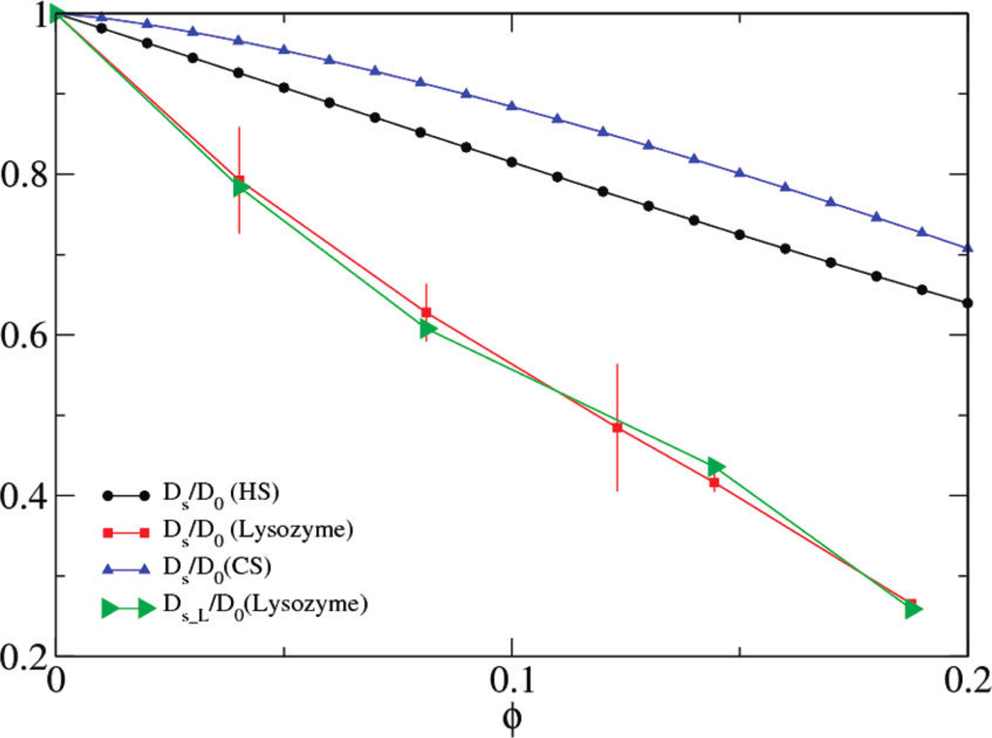
The competition of more types of interactions can lead to the formation of kinds of clusters in protein solutions differing e.g. in the lifetime, or in the stiffness. However, the variety of phenomena arising from such pair potentials is very broad, and in the same system more than one may occur, depending for instance on the time- and length scale of observation. As an example, Cardinaux et al. (Reference Cardinaux, Zaccarelli, Stradner, Bucciarelli, Farago, Egelhaaf, Sciortino and Schurtenberger2011) identified an arrest transition at volume fractions  $\varphi {\rm \mathbin{\lower.3ex\hbox{$\buildrel\gt\over {\smash{\scriptstyle\sim}\vphantom{_x}}$}}} 0.26$ in Lys solutions by combining SAXS, NSE and rheology experiments. In addition to this, the authors employed molecular and Brownian dynamics simulations using effective pair potential among proteins based on the combination of short-range attraction and long-range repulsion. Such simulations suggested that the experimentally observed arrest is driven by the slowing down of the motion of clusters (Cardinaux et al., Reference Cardinaux, Zaccarelli, Stradner, Bucciarelli, Farago, Egelhaaf, Sciortino and Schurtenberger2011). In particular, a transition from a suspension dominated by monomers to one dominated by transient clusters was obtained at volume fractions larger than φ ~ 0.05. However, at higher volume fractions, simulations still predicted transient clusters, even though NSE measurements indicated that the cluster lifetime was becoming increasingly large, as evinced by the fact that the dynamic structure factor became almost independent of q for q >q c, where q c is the wavevector at which a cluster–cluster correlation peak is observed in S(q) from SAXS (Cardinaux et al., Reference Cardinaux, Zaccarelli, Stradner, Bucciarelli, Farago, Egelhaaf, Sciortino and Schurtenberger2011).
Godfrin et al. (Reference Godfrin, Hudson, Hong, Porcar, Falus, Wagner and Liu2015) also noticed that, while viscosity measurements on Lys in aqueous solutions show a behavior typical for Newtonian liquids, at high concentration the short-time dynamics measured by NSE is characterized by features typical of glassy colloid systems. Moreover, with increasing protein concentration, a correlation peak grows in the SANS data, the so-called intermediate range order peak (IRO, observed first by Stradner et al., Reference Stradner, Sedgwick, Cardinaux, Poon, Egelhaaf and Schurtenberger2004), also referred to as cluster–cluster correlation peak in previous studies. This behavior was explained by Godfrin and co-workers as a consequence of localized heterogeneous density distributions occurring at the same length-scale at which the IRO peak is detected, due in turn to competing short-range attractive and long-range repulsive interactions (Godfrin et al., Reference Godfrin, Hudson, Hong, Porcar, Falus, Wagner and Liu2015).
Recently, Riest et al. (Reference Riest, Nägele, Liu, Wagner and Godfrin2018) have also tested a semi-analytic theoretical method predicting diffusion properties and viscosity in isotropic particle suspensions to low-salinity Lys protein solutions, using a short-range attractive plus long-range repulsive potential. Monte Carlo simulations representing seven lysozyme samples indicated that Lys in these systems is either in a dispersed fluid or in random percolated states. The obtained theoretical predictions for the hydrodynamic function were in quantitative agreement with experimental NSE data up to φ ~ 0.04, also featuring an IRO peak. Significant differences at higher concentrations and low temperatures were suggested to be due to translational–rotational diffusion coupling induced by the shape and interaction anisotropy of particles and clusters, patchiness of the Lys particle surfaces, and the intra-cluster dynamics, which were not included in the theoretical model (Riest et al., Reference Riest, Nägele, Liu, Wagner and Godfrin2018). Nevertheless, such a simplified model may be of interest for predicting and identifying trends in the structure, short-time diffusion and rheology of globular protein solutions as a function of different interaction and system parameters (Riest et al., Reference Riest, Nägele, Liu, Wagner and Godfrin2018).
The formation of increasingly large clusters as a function of protein concentration is rather often observed (although also the opposite, that is a decreased aggregation at high concentrations, has been observed; see e.g. Da Vela et al. (Reference Da Vela, Roosen-Runge, Skoda, Jacobs, Seydel, Frielinghaus, Sztucki, Schweins, Zhang and Schreiber2017) for γ-globulin). For instance, clusters of bovine beta-lactoglobulin (BLG) were investigated with SAXS as well as NSE and NBS spectroscopy by Braun et al. (Reference Braun, Grimaldo, Roosen-Runge, Hoffmann, Czakkel, Sztucki, Zhang, Schreiber and Seydel2017), and a monotonous increase of the average hydrodynamic cluster radius was observed over a broad protein concentration range, corresponding to oligomeric structures of BLG ranging from the native dimers up to roughly four dimers. The combination of static and dynamic measurements suggested that the clusters are compact and have a lifetime that is larger than both the NSE and NBS observation timescales, that is up to ~50 ns (Braun et al., Reference Braun, Grimaldo, Roosen-Runge, Hoffmann, Czakkel, Sztucki, Zhang, Schreiber and Seydel2017). The authors further reported that an SLS/DLS study by Piazza and Iacopini (Reference Piazza and Iacopini2002) on a specific type of BLG (bovine β-lactalbumin A) indicated the formation of oligomer-type ‘transient’ clusters with a limited lifetime on the microsecond observation timescale, consistent with PFG-NMR results on millisecond timescales by Le Bon et al. (Reference Le Bon, Nicolai, Kuil and Hollander1999), indicating that BLG self-diffusion in concentrated solutions is in agreement with that of dimers. A recent all-atom MD investigation of the dynamics of chicken villin headpiece HP-36 at concentrations ranging from ~30 up to ~130 mg ml−1 by Nawrocki et al. (Reference Nawrocki, Wang, Yu, Sugita and Feig2017) yielded similar results and provided further insight into the possible mechanism of formation of these clusters. After adjusting the force-field to increase the protein–water interactions and reproduce the expected dilute limit translational and rotational diffusion coefficients, the concentration of villin was increased and the formation of transient clusters was observed. The clusters were characterized by a size distribution moving to larger sizes and by an increasing lifetime (up to some hundreds of nanoseconds) with rising protein concentration. Other than in the approach by Braun et al. (Reference Braun, Grimaldo, Roosen-Runge, Hoffmann, Czakkel, Sztucki, Zhang, Schreiber and Seydel2017), Nawrocki and collaborators found in their simulations that the formation of clusters alone nearly completely accounts for the obtained slowing down of the translational diffusion of villin (Nawrocki et al., Reference Nawrocki, Wang, Yu, Sugita and Feig2017). For rotational diffusion, a somewhat more pronounced effect was observed. Finally, the authors also found that the residues involved in protein–protein binding were largely acidic and basic, which, was argued, suggests that the assembly of nonspecific clusters may be driven by electrostatic interactions and salt-bridge formation (Nawrocki et al., Reference Nawrocki, Wang, Yu, Sugita and Feig2017).
Yearley et al. (Reference Yearley, Godfrin, Perevozchikova, Zhang, Falus, Porcar, Nagao, Curtis, Gawande, Taing, Zarraga, Wagner and Liu2014) observed by NSE the formation of protein clusters even in solutions of monoclonal antibodies (mAbs) at high concentrations. In their study, two model mAbs in solution were compared, one of which was characterized by a steep increase of the viscosity of solutions at high concentration (mAb1), the other showing a less pronounced increase (mAb2). The combination of NSE and small-angle scattering demonstrated that in the solutions with high viscosity the mAb1 molecules formed dimers, whereas the mAb2 molecules retained their monomer structure. The high viscosity, which is undesirable for pharmaceutical applications, was therefore related to the formation of such dimers at high concentrations (Yearley et al., Reference Yearley, Godfrin, Perevozchikova, Zhang, Falus, Porcar, Nagao, Curtis, Gawande, Taing, Zarraga, Wagner and Liu2014).
Understanding protein aggregation is fundamental also because it often leads to the formation of the so-called amyloid fibrils, which are related to numerous diseases. In this context, Erlkamp et al. (Reference Erlkamp, Grobelny, Faraone, Czeslik and Winter2014) performed a combined SAXS-NSE study of insulin under two solvent different conditions, one promoting, and the other inhibiting amyloid fibril formation. In the former case, no collective diffusion (density fluctuations) was observed in the range of time and length scales experimentally accessible, and only self-diffusion could be measured. In the latter case, collective diffusion was visible, along with an appearance of a correlation peak in the SAXS profiles. The results suggested therefore that a lack of repulsive interactions reducing collective effects promotes the fibril formation (Erlkamp et al., Reference Erlkamp, Grobelny, Faraone, Czeslik and Winter2014).
The formation of amyloid fibrils by an IDP, αSN, was shown to be involved in the pathogenesis of Parkinson's disease, which motivated an NBS study by Fujiwara et al. (Reference Fujiwara, Araki, Matsuo, Yagi, Yamada, Shibata and Mochizuki2016). The authors were able to measure the dynamics of 9.5 mg ml−1 purified αSN, and that of 46 mg ml−1 αSN in the fibril state in D2O. Such measurements are remarkable for NBS, since this technique usually requires rather large protein concentrations to obtain a reasonable signal-to-noise ratio. The detection of low quantities of proteins is challenging and is only possible in latest, state of the art spectrometers. Fujiwara et al. (Reference Fujiwara, Araki, Matsuo, Yagi, Yamada, Shibata and Mochizuki2016) found that the αSN in its monomeric state undergoes diffusive global motions, which are instead largely suppressed in the fibril state. In contrast, the amplitude of the side-chain motion was found to be larger in the fibril state than in the monomeric state (Fujiwara et al., Reference Fujiwara, Araki, Matsuo, Yagi, Yamada, Shibata and Mochizuki2016). It was concluded by the authors that, within the fibrils, a significant space is left for the solvent, which allows for a large a distribution of conformations of αSN side-chains. Moreover, it was pointed out that the larger amplitude of the side-chain motion in the fibril state compared with the monomeric state implies that the fibril state is entropically favorable (Fujiwara et al., Reference Fujiwara, Araki, Matsuo, Yagi, Yamada, Shibata and Mochizuki2016).
Other non-neutron based techniques such as DLS (Bolañnos-García et al., Reference Bolanños-García, Mas-Oliva, Soriano-García and Moreno1998; Li et al., Reference Li, Lubchenko and Vekilov2011; Arzenšek et al., Reference Arzenšek, Kuzman and Podgornik2012; Soraruf et al., Reference Soraruf, Roosen-Runge, Grimaldo, Zanini, Schweins, Seydel, Zhang, Roth, Oettel and Schreiber2014; Maes et al., Reference Maes, Vorontsova, Potenza, Sanvito, Sleutel, Giglio and Vekilov2015; Bauer et al., Reference Bauer, Göbel, Schwab, Schermeyer and Hubbuch2016), DLS combined with Raman spectroscopy (Lewis et al., Reference Lewis, Qi, Kidder, Amin, Kenyon and Blake2014) or with NMR (Poznański et al., Reference Poznański, Szymaǹski, Basiǹska, Słomkowski and Zielenkiewicz2005), fluorescence spectroscopy (Nath et al., Reference Nath, Meuvis, Hendrix, Carl and Engelborghs2010; Roberti et al., Reference Roberti, Jovin and Jares-Erijman2011; Nath and Rhoades, Reference Nath and Rhoades2013) and rheology (Dharmaraj et al., Reference Dharmaraj, Godfrin, Liu and Hudson2016), as well as simulations (Bratko et al., Reference Bratko, Cellmer, Prausnitz and Blanch2007) can be used to study the dynamics of systems with aggregating proteins. One of the strengths of the combination of such techniques with neutron scattering related to the different accessible times, is the potential of inferring information on the type and lifetime of clusters (as in Liu et al., Reference Liu, Porcar, Chen, Chen, Falus, Faraone, Fratini, Hong and Baglioni2010) and aggregates on wide concentration ranges, as well as on the kinetics of the process.
Several types of isotropic and anisotropic interactions between proteins exist, with different typical ranges and strengths. One of these anisotropic interactions arises as a consequence of the highly heterogeneous surface charge pattern of proteins, such that, in some cases, proteins could be successfully modeled as hard spheres with attractive patches (Gögelein et al., Reference Gögelein, Nägele, Tuinier, Gibaud, Stradner and Schurtenberger2008; Roosen-Runge et al., Reference Roosen-Runge, Zhang, Schreiber and Roth2014). In an NBS study on the dynamics of BSA in the presence of the trivalent salt YCl3, Grimaldo et al. (Reference Grimaldo, Roosen-Runge, Hennig, Zanini, Zhang, Zamponi, Jalarvo, Schreiber and Seydel2015b) found that, at several fixed protein concentrations c p and a series of salt concentrations c s, the apparent diffusion coefficient of BSA D(c s, c p) normalized by D(c s = 0, c p) decreases as a function of the number c s/c p of ions of Y3+ per protein in a remarkably universal manner with respect to c p. The authors interpreted such a result in terms of a model of ion-activated patchy hard spheres (Roosen-Runge et al., Reference Roosen-Runge, Zhang, Schreiber and Roth2014), and suggested that the observations could be explained by the formation of protein clusters with a given size-distribution mediated by Y3+ ions binding semi-quantitatively to specific sites on the protein surface (Grimaldo et al., Reference Grimaldo, Roosen-Runge, Hennig, Zanini, Zhang, Zamponi, Jalarvo, Schreiber and Seydel2015b). Such a result complemented a previous DLS study on the same system, but at smaller protein concentrations and corroborated the hypothesis that the formation of clusters could be observed by light scattering when increasing c s/c p (Soraruf et al., Reference Soraruf, Roosen-Runge, Grimaldo, Zanini, Schweins, Seydel, Zhang, Roth, Oettel and Schreiber2014).
In many globular proteins competing interactions can lead, in addition to cluster formation, to liquid–liquid phase separation at low temperatures, as in the case of γ B-crystallin. The collective diffusion of proteins in such a system was investigated by Bucciarelli et al. (Reference Bucciarelli, Casal-Dujat, De Michele, Sciortino, Dhont, Bergenholtz, Farago, Schurtenberger and Stradner2015) with a combination of DLS and NBS. The authors found that the combination of critical slowing down and dynamical arrest results in a peculiar wavevector dependence of the dynamic structure factor I(q,t), even though the static properties such as the osmotic compressibility and the static correlation length are in quantitative agreement with predictions for binary liquid mixtures (Bucciarelli et al., Reference Bucciarelli, Casal-Dujat, De Michele, Sciortino, Dhont, Bergenholtz, Farago, Schurtenberger and Stradner2015). Later studies combining NSE experiments with CG simulations (Bucciarelli et al., Reference Bucciarelli, Myung, Farago, Das, Vliegenthart, Holderer, Winkler, Schurtenberger, Gompper and Stradner2016; Myung et al., Reference Myung, Roosen-Runge, Winkler, Gompper, Schurtenberger and Stradner2018) indicated that a major role in determining S(q, t) and hence collective diffusion might be played by the presence of attractive patches on the protein surface and nonspherical shape (see also section ‘Global diffusion’).
In summary, the combination of static and dynamic techniques was shown to provide important information on microscopic properties such as clustering and phase transitions useful to understand the basis of macroscopic properties of the system. From the perspective of colloid science, proteins represent a fascinating model system and an opportunity for the study of new phenomena related to the interplay of repulsive and attractive, potentially anisotropic interactions (Riest and Nägele, Reference Riest and Nägele2015; Sentjabrskaja et al., Reference Sentjabrskaja, Zaccarelli, De Michele, Sciortino, Tartaglia, Voigtmann, Egelhaaf and Laurati2016; Das et al., Reference Das, Riest, Winkler, Gompper, Dhont and Nägele2018; Myung et al., Reference Myung, Roosen-Runge, Winkler, Gompper, Schurtenberger and Stradner2018).
Concluding remarks
From the reviewed work employing neutron spectroscopy and complementary techniques to explore proteins in liquid solutions, three aspects have become undoubtedly clear:
• Protein dynamics occurs on multiple hierarchical time and length scales.
• Different experimental techniques, each having specific advantages and disadvantages, access different types of dynamics and, hence, are complementary (see Table 1).
• Protein dynamics is related to protein function.
The review has focused on neutron spectroscopy while mentioning complementary methods in a non-exhaustive manner to highlight where neutron spectroscopy, to their advantage or disadvantage, differ from these other methods. For instance, the access to short-time center-of-mass diffusive dynamics in protein solutions is part of the advantages of employing neutron spectroscopy, by providing a unique probe to global dynamics on a timescale before this dynamics is altered by protein–protein collisions. However, it is generally necessary to use D2O as a solvent to focus on the incoherent signal from protonated proteins. D2O solvent may alter the dynamics of the proteins themselves beyond the sole effect of the different viscosity compared with H2O.
In liquid protein solutions, mainly the diffusive dynamics has been explored using QENS, accessing picosecond to nanosecond timescales and nanometer length scales. Moreover, diffusive dynamics on longer time- and length-scales has been explored using NSE spectroscopy. Our review has attempted but certainly not attained a comprehensive overview of these studies addressing diffusive dynamics in liquid protein solutions using neutrons. In contrast, besides the above-mentioned complementary methods, also the deep inelastic neutron scattering accessing high-frequency vibrational dynamics (in the THz range and beyond) could not be addressed in any detail within the limited scope of this review.
Among the unique properties of neutron spectroscopy experiments, we highlight the possibility to benefit from the information contained in incoherent scattering to infer on ensemble-averaged localized dynamics. This information on the geometrical confinement of a diffusive process indirectly provides knowledge on local order in proteins which – outside crystals – generally do not display any long-range order. In liquid solutions of proteins, both the coherent and incoherent scattering can be interesting, and many NSE experiments on protein solutions are based on the coherent part of the signal. For instance, information on dynamic or transient protein cluster formation can be enhanced by combining both coherent (NSE, on longer length scales) and incoherent (NBS, on shorter length scales) scattering experiments.
Despite the substantial efforts and number of studies carried out in the past few decades on protein dynamics, several questions remain at least partially unanswered. The hierarchical nature of protein dynamics in relation to the protein function, the role of the structure, the binding of different ligands, the state of a protein in determining the protein internal dynamics and the impact of different local cellular environments, as well as anisotropic pair potentials or particles shapes on the global protein dynamics are all topics still lacking a deep, fundamental understanding. As seen in this review, to tackle these problems a great flexibility regarding both the type of probed atoms or groups of atoms and the observation timescales is required. For this reason, we believe that, in the near future, studies combining different experimental techniques such as neutron scattering, NMR, fluorescence spectroscopy, light scattering and profiting from MD simulations will be essential to provide a substantial thrust to several fields of biological physics. Recent improvements as well as new neutron scattering instruments will also open new perspectives. Future topics of great interest include kinetic studies of dynamics during processes such as macromolecular assembly formation, in situ crystallization and cluster formation.
Summary
Protein dynamics is a key research area in biophysics with many facets in terms of time and length scales as well as implications for physical properties and biological function. Neutron scattering spectroscopy was employed in a multitude of investigations of protein dynamics – from fast, localized motion with TOF and NBS to slow domain motion with NSE, as well as center-of-mass diffusion with NBS and NSE. In this context, neutron spectroscopy has benefited from progress in neutron instrumentation and data analysis during the recent years. With its nondestructive and contact-free access to a wide range of time and length scales accessing the molecular level, including in optically opaque samples, the neutron scattering technique has proven to be complementary to other established biophysical techniques such as NMR, fluorescence spectroscopy and light scattering. By probing both the coherent and incoherent scattering, it can measure both collective and self-dynamics. Among the emerging topics of research, the center-of-mass and internal dynamics in crowded protein solutions, the formation of static or transient protein clusters, and more generally protein self-assembly in solution may be named. Experiments have shown that the internal motion of proteins in hydrated powders differs from that in solution, where generally additional dynamics was observed. Protein internal dynamics does not only depend on the hydration level, but also on the characteristics of the solvent, e.g. if H2O or D2O are used. EINS studies revealed the existence of a dynamical transition in solution similar to that observed in powders. Other than in powders, some results suggested an apparent decoupling of water and protein dynamics. Furthermore, numerous studies have demonstrated an effect of the structure and state of proteins, as well as an influence of pressure, temperature and crowding, on their dynamic behavior. Finally, in addition to studies on highly concentrated protein solutions, investigations of entire living cells demonstrated the occurrence of different dynamical processes in vivo, and provided evidence for a molecular mechanism of adaptation of organisms to the temperature at which they live.
Author ORCIDs
Marco Grimaldo: 0000-0002-3772-7137, Felix Roosen-Runge, 0000-0001-5106-4360, Fajun Zhang, 0000-0001-7639-8594, Frank Schreiber, 0000-0003-3659-6718, Tilo Seydel, 0000-0001-9630-1630
Acknowledgements
The authors are indebted to many collaborators, with whom it has been a pleasure to interact. These include in particular present and former members of the Tübingen-ILL collaboration. The authors would like to thank in particular H. Schober, B. Farago and B. Frick for discussions and support. Fruitful interactions with A. Stadler, R. Biehl, I. Hoffmann, V. Garcia Sakai, G. Kneller, J. Peters, K. Saalwächter, A. Stradner and P. Schurtenberger are also gratefully acknowledged. The authors would like to acknowledge enlightening discussions with numerous colleagues in the field, who cannot all be mentioned. We thank C. Beck, O. Matsarskaia, M. Braun, M. Oettel, R. Roth and E. Schäffer for stimulating discussions. The authors wish to thank the ILL (Grenoble), the JCNS (Jülich), FRM-II (Munich) and SNS (Oak Ridge) for making our own neutron-based work on proteins in solution possible. Finally, this work would not have been possible without the support (in part) of the Deutsche Forschungsgemeinschaft (DFG), the Agence Nationale de la Recherche (Project ID: ANR-16-CE92-0009 ‘ImmunoglobulinCrowding’), the ILL and the Studienstiftung des Deutschen Volkes.

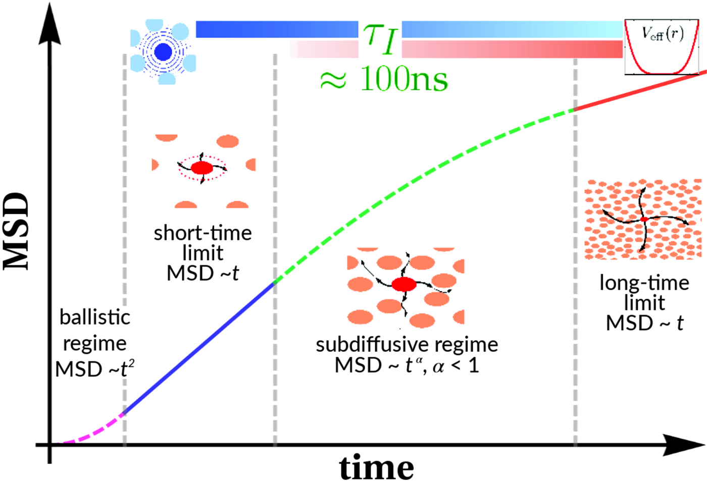


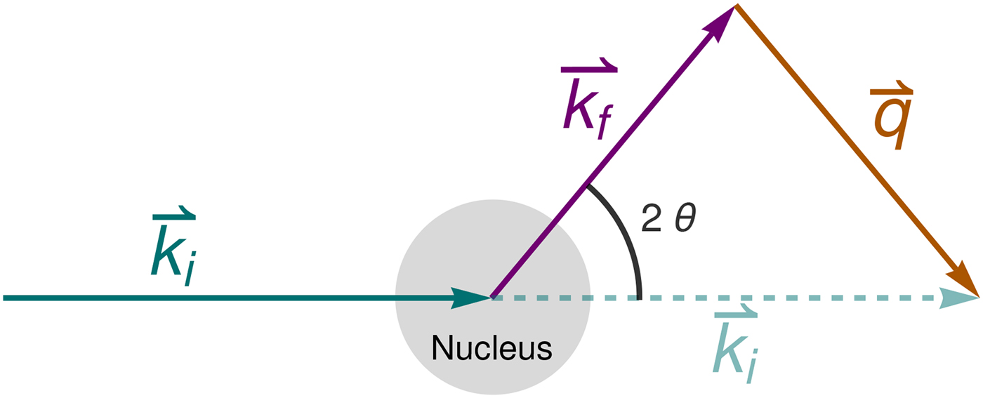


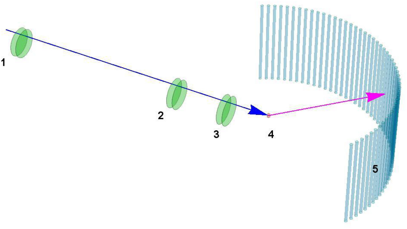


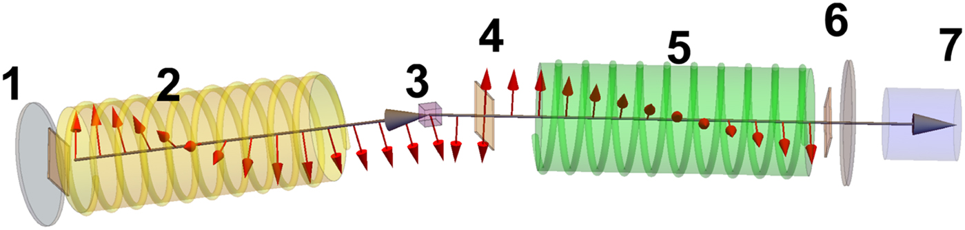


 Open access

