


1 INTRODUCTION
Since its astronomical discovery in 1970 (Wilson, Jefferts, & Penzias Reference Wilson, Jefferts and Penzias1970), the carbon monoxide (CO) molecule has been utilised as a key tracer of molecular gas in the Galaxy. Second in numerical abundance only to the H2 molecule, the large abundance (~10−4) and low electric dipole moment (0.122 D) of CO allow cold molecular gas to be well-traced by the J = 1–0 rotational transition. CO surveys of the molecular gas in the Galactic Plane can help shape an understanding of star formation, dynamics, and chemistry within the Milky Way.
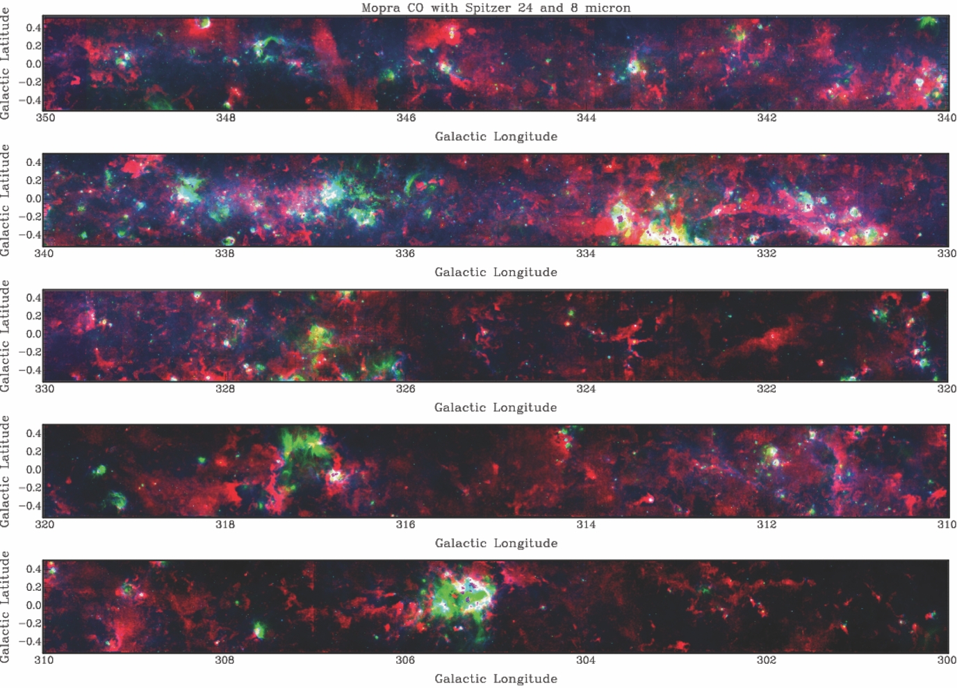
The Mopra Galactic Plane CO survey is the highest resolution large-scale three-dimensional molecular gas survey of the inner Galactic Plane so far. With this paper, we publicly release COFootnote 1, 13CO, and C18O(1–0) dataFootnote 2 for the region from l = 300 to 350°, and b = ±0.5° (see Figure 1). This release encompasses updated reductions of data contained within the previous Mopra CO data releases (Burton et al. Reference Burton2013; Braiding et al. Reference Braiding2015) and, along with the Mopra CO maps of the Carina/Gum 31 region (Rebolledo et al. Reference Rebolledo2016) and the Central Molecular Zone (CMZ, Blackwell et al. in preparation), will eventually be incorporated into a larger mosaic with coverage spanning longitude l ~260 to +11° and a latitudinal range of ±1°. Additional targeted extensions beyond 1° will also be included.
Three-colour image of the Galactic Plane from the Mopra CO survey (red; peak intensity image from v = −150 to +50 km s−1) together with the Spitzer MIPSGAL 24 μm (green; Carey et al. (Reference Carey2009)) and GLIMPSE 8 μm (blue; Churchwell et al. (Reference Churchwell2009); Benjamin et al. (Reference Benjamin2003)) surveys.
The Columbia CO(1–0) survey (Dame, Hartmann, & Thaddeus Reference Dame, Hartmann and Thaddeus2001) has been a revolutionary tool for the study of the Milky Way, its 8-arcmin resolution has helped enable a large number of important astronomical results. Some examples include the constraining of the CO X-factor and Galactic cloud masses, the identification of Galactic structures (e.g. Dame & Thaddeus Reference Dame and Thaddeus2011; Vallée Reference Vallée2014) and implications for dark matter research (e.g. Drlica-Wagner et al. Reference Drlica-Wagner, Gómez-Vargas, Hewitt, Linden and Tibaldo2014).
The Mopra Galactic Plane CO survey will enable new Galactic science. ALMA offers arcsecond-level spatial resolution in the CO(1–0) transition (e.g. Mathews et al. Reference Mathews2013), and the very fine field of view of ALMA is well-complemented by a large sub-arcminute-scale map which can allow the identification of molecular gas components for observations. Furthermore, comprehensive investigations of the ‘missing’ gas of the Galaxy (as inferred from dust and gamma-ray observations, e.g. Planck Collaboration et al. 2015) require molecular clouds to be imaged at a resolution able to separate these ‘dark’ components, complementing observatories such as the Cherenkov Telescope Array (CTA, Cherenkov Telescope Array Consortium et al. 2017) and the High Elevation Antarctic Telescope (HEAT, Walker et al. Reference Walker and Oschmann2004). Our survey also goes one step further than historical 12CO surveys of the Galactic Plane by mapping multiple CO isotopologues that probe the regions where CO(1–0) becomes optically thick, tracing additional mass components.
In this paper, we present 50 deg2 of Mopra 12CO, 13CO, C18O, and C17O data. Section 3 is an update on the data-processing techniques used by the survey, descriptions of the data quality, and a list of regions affected by contaminated reference positions. A series of images and characterisations of Mopra data are presented in Section 4 alongside a new catalogue of C18O clumps located within the region l = 330–340°. Finally, we outline recent region and source-specific investigations that utilise Mopra CO isotopologue data and propose additional work to be performed, in conjunction with other surveys, to determine the evolution of molecular clouds, and the origins of cosmic rays (CRs) (Sections 5 and 6).
2 PREVIOUS DATA RELEASES
The Mopra CO Galactic Plane survey was first described in Burton et al. (Reference Burton2013), which presented the results of the pilot observations undertaken in 2011 March of the single square degree, l = 323–324°, b = ±0.5°. The aims and the approach of the Mopra CO survey were also discussed in detail, with science goals of comparing the emission of Gamma and CRs to emission from nearby molecular clouds, and characterising the formation of molecular clouds. The initial observations were used to describe a number of giant molecular clouds along the G323 line of sight, demonstrating how the multiple isotopologue CO survey data could be used in conjunction with H i data from the Southern Galactic Plane Survey (SGPS; McClure-Griffiths et al. Reference McClure-Griffiths, Dickey, Gaensler, Green, Haverkorn and Strasser2005) to determine the mass and column densities within these clouds. This data remains some of the noisiest in the Mopra CO survey (see Figures 2–4), as the initial observations were conducted during summer months.
1 σ noise images for the 12CO data covering the full 50 deg2 from l = 300–350° in units of T*A (K) (as indicated by the scale bars). The striping pattern is inherent to the data set, resulting from scanning in the l and b directions in variable observing conditions.

As in Figure 2, these are the 1 σ noise images for the 13CO data covering the full 50 deg2 from l = 300–350° in units of T*A (K) (as indicated by the scale bars).

As in Figure 2, these are the 1 σ noise images for the C18O data covering the full 50 deg2 from l = 300–350° in units of T*A (K) (as indicated by the scale bars).

The first data release by Braiding et al. (Reference Braiding2015, hereafter DR1), presented the first 10° of the Mopra CO survey, covering Galactic longitudes l = 320–330° and latitudes b = ±0.5°, and l = 327–330°, b = −0.5–+1.0°. The maps possessed a typical rms noise of ~1.2 K in the 12CO data and ~0.5 K in the other isotopologue frequency bands. It was noted that the line intensities from the Mopra CO survey are ~1.3 times higher than those of Dame et al. (Reference Dame, Hartmann and Thaddeus2001, see also Section 4.1), although the average line profiles for each square degree show similar qualitative features. The calculated mass of the molecular clouds in the 10 deg2 of DR1 was found to be ~4 × 10⁷ M⊙, and included many complex filamentary structures from the tangent point to the Norma spiral arm of the Galaxy. Data release 3 contains an improved reduction of these 10 deg2, and although the changes are very minor (~1% of voxels differ from their previous values, most by ≪0.1 K), it is recommended that current Mopra CO users download the newer files for future work.
Data release 2 (DR2; Rebolledo et al. Reference Rebolledo2016) comprised 8 deg2 of observations covering the Carina Nebula and Gum 31 molecular complex. In addition to the molecular gas distribution derived from 12CO and 13CO line emission maps, this paper presented total gas column density and dust temperature maps. The Mopra CO data were complemented by dust maps from Herschel (Molinari et al. Reference Molinari2010), allowing the calculation of dust column densities within the nebula of between 6.3× 10²⁰ and 1.4× 1023 cm−2, and dust temperatures within a range of 17 to 43 K. The distribution of the total gas is well represented by a lognormal function, but a tail at high densities is clearly observed, which is a common feature of nebulae with active star formation (Pineda et al. Reference Pineda, Goldsmith, Chapman, Snell, Li, Cambrésy and Brunt2010; Rebolledo et al. Reference Rebolledo2016). Regional variations in the masses recovered from the Mopra CO emission and Herschel dust maps revealed the different evolutionary stages of the molecular clouds that comprise the Carina Nebula–Gum 31 complex.
The CMZ of the Galaxy contains dense (e.g. Jones et al. Reference Jones2012, Reference Jones, Burton, Cunningham, Tothill and Walsh2013), high-temperature (e.g. Ao et al. Reference Ao2013) molecular clouds with a total cumulative mass of ~5 × 10⁷ M⊙ (e.g. Pierce-Price et al. Reference Pierce-Price2000). The fourth data release of the Mopra CO survey will cover the Galactic Centre region [358.5 ⩽ l ⩽ 3.5°, −0.5 ⩽ b ⩽ +1.0°; Blackwell et al. (in preparation)], which has required the development of new observing and data processing techniques to produce high-quality spectral maps. As the star-formation behaviour of molecular clouds in the CMZ is linked to their orbital dynamics (e.g. Kruijssen, Dale, & Longmore Reference Kruijssen, Dale and Longmore2015), the high-resolution Mopra CO maps will enable new studies of the inner Galaxy gas dynamics and triggered star formation.
3 DATA RELEASE 3
Observations for this data release were carried out over the Southern Hemisphere winters of 2011–2016 using Mopra, a 22-m single-dish radio telescope located ~450-km north-west of Sydney, Australia (at 31°16′04″ S, 149°05′59″ E, 866 m a.s.l.). Observations utilised the UNSW Digital Filter Bank (the UNSW-MOPS) in its ‘zoom’ mode, with 8×137.5 MHz dual-polarisation bands. These bands were tuned to target the J=1–0 transition of 12CO, 13CO, C18O, and C17O (with central frequencies of 115271.202, 110201.354, 109782.176, and 112358.988 MHz, respectively). Three bands were tuned to sample a 12CO(1–0) velocity coverage of ~1 100 km s−1, while the 13CO(1–0) and C18O(1–0) transitions each had two dedicated bands to sample a velocity-coverage of ~770 km s−1. One band was allocated to the least-abundant molecular transition, C17O(1–0), resulting in ~380 km s−1 of velocity coverage. The targeted central frequencies were offset according to Galactic Longitude to maximise overlap with expected Galactic rotation velocities. As in DR1, the observations from l = 323–331°, b = ±0.5° cover a smaller velocity range, as only four ‘zoom’ bands were utilised during the 2011 observing period, one for each isotopologue. Our observations across the full 50 deg2 of DR3 suggest that it is unlikely that there are any high-velocity clouds in this region, as all of the 12CO clouds detected to date have been within the velocity range of the primary zoom band.
As described in Burton et al. (Reference Burton2013), Fast-On-The-Fly (FOTF) mapping has been carried out in 1 deg2 segments, with each segment being comprised of orthogonal scans (in longitudinal and latitudinal directions) to reduce scanning artefacts. The exposure of each square degree is at least ~20 h, more in places where poor weather or technical issues interrupted observations and triggered a repeat of the affected scans.
The angular resolution of the Mopra beam at 115 GHz is 33-arcsec FWHM (Ladd et al. Reference Ladd, Purcell, Wong and Robertson2005); after a median filter convolution is applied during the data reduction process, the dataset possesses a beam size of around 0.6 arcmin. Since the survey region is spatially fully sampled, the extended beam efficiency, ηXB = 0.55 at 115 GHz, should be used to convert brightness temperatures into line fluxes (rather than the main beam efficiency ηMB = 0.42; Ladd et al. Reference Ladd, Purcell, Wong and Robertson2005).
DR3 has been made available at the survey website and in the PASA data archive as a series of fits files covering a square degree for each isotopologue, separated by half a degree along the Galactic Plane. Although the full range of velocity space available for 12CO is [−1 000,+1 000] km s−1 (with file sizes of ~800 MB deg−2), it is expected that most users would prefer to download the smaller (~300 MB per deg−2) files covering the velocity range [−150, +50] km s−1 illustrated in this paper. No emission has as yet been detected outside this range, although closer to the Galactic centre this range will be extended. Also available are the T sys, beam coverage, and RMS noise images for each line.
3.1. Data processing
From 2015 September, observations were affected by a recurring synchronisation loss between the telescope and spectrometer, creating a spike in the central channel of ~0.03% of spectra. This was not automatically flagged by software during observations or using the data reduction processes from DR1 and DR2, and if left unchecked these artefacts would propagate throughout the reduction, particularly when spikes appeared in the sky reference spectra. A new IDL routine was created to mask the affected channels in the raw data from the telescope; by coincidence, this also flags other poor spectra caused by clouds or system fluctuations.
The rest of the data reduction remains unchanged from DR1 and DR2, involving six main stages of processing (Braiding et al. Reference Braiding2015; Rebolledo et al. Reference Rebolledo2016). First, LIVEDATAFootnote 3 (Gooch Reference Gooch, Jacoby and Barnes1996) was used to perform the band-pass correction and background subtraction using data from the nearest reference position to create the calibrated spectra. These are then analysed using an IDL routine that flags any spectra that are poorly calibrated or particularly noisy (mostly in the 12CO bands where the system temperature is higher). The data are then interpolated onto a uniform grid using GRIDZILLA (Gooch Reference Gooch, Jacoby and Barnes1996), employing a median filter for the interpolation of the oversampled data onto each grid location. GRIDZILLA excludes from the grid those spectra for which the T sys values are above 1 000 K for the 12CO cube, and 700 K for the other lines (see Section 3.2). The output of these processes is a fits data cube in (l, b, and V LSR) coordinates.
Noisy outlier pixels, rows, and columns are then cleaned using an IDL routine that first detects voxels that differ from their neighbours by more than five standard deviations, then rows and columns where the mean spectra differs by more than three standard deviations from the median of the entire data set (typically caused by the passage of clouds during the sky reference measurement). These ‘bad’ data are replaced by interpolating the values of their neighbouring pixels, as described in Burton et al. (Reference Burton2013), and the process is repeated until no further ‘bad’ data are detected.
The data are then continuum-subtracted using first a fourth-order and then a seventh-order polynomical fit, to yield data cubes of the brightness temperature for each spectral line as a function of Galactic coordinate and V LSR velocity. Finally, data cubes that have been affected by contamination from faint molecular clouds present within the reference position (see Section 3.3), are corrected by modelling the contaminant component and adding that back into the final clean spectrum (Braiding et al. Reference Braiding2015).
3.2. Data quality
The observations for DR3 were carried out over a wide variety of weather conditions, ranging from those of late Southern Hemisphere summer (March 2011, 2014, and 2015) when the system temperature was high (~900 K for 12CO) to deep winter (2011–2016) where the conditions are quite stable and T sys in the 12CO band is quite stable at around 400 K. This is reflected in the noise maps of the 12CO, 13CO, and C18O data, which are presented in Figures 2–4, respectively. The noise value for each pixel was determined from the standard deviation of the continuum channels for line-of-sight velocities containing no apparent signal. The thick striping seen within these maps is an effect of scanning in l and b directions under different system temperatures and observing conditions. Thinner stripes and spots of low noise indicate the positions of ‘bad’ pixels, rows, or columns that were identified and interpolated over (see Section 3.1; Burton et al. Reference Burton2013).
The system temperature of Mopra (T sys, discussed further in Appendix A.2) reflects the total level of signal received from the instrument, telescope, and sky, in addition to that from the source (which contributes a near-insignificant portion to T sys). It is calibrated with reference to an ambient temperature paddle every 30 min, allowing us to control for variations in the weather. Observations with an average T sys greater than 1 000 K were repeated under better weather conditions, while any individual measurement which possessed a T sys greater than 1 000 K was filtered out during the imaging stage of the data reduction (see Section 3.1).
To examine the Mopra beam resolution, observations of SiO(2−1,v=1) maser emission from the red supergiant variable star, AH Scorpii, were taken in 2017 November (Figure 9 in Section A.1). The data were integrated over all masers in velocity-space, and gaussian line profiles were fitted to the diametral distribution in both right-ascension and declination. The measured FWHM was then deconvolved with the map smoothing by subtracting the smoothing kernal FWHM in quadrature. The resultant Mopra beam FWHM was calculated to be 35arcsec ± 1 arcsec and 34arcsec ± 1 arcsec for the Mopra beam axis at 86 GHz. This is consistent with previous calibration measurements that characterised the Mopra beam FWHM as 36arcsec ±3 arcsec (Ladd et al. Reference Ladd, Purcell, Wong and Robertson2005).
3.3. Sky reference positions
Table 1 lists coordinates of the sky reference positions used for each square degree of observations. Several of these reference positions contained 12CO, 13CO, and in at least one instance C18O line emission, which propagate into the data cubes as negative ‘emission’. The line of sight velocity and peak intensity of the reference position 12CO line emission are included in Table 1, the 13CO line emission is typically fainter than the 12CO line by a factor of 5, and similarly C18O emission is only detected when the 12CO contamination is exceptionally bright.
Sky reference beam positions for each square degree of DR3. Several cubes were contaminated by negative 12CO, 13CO and C18O line emission from the sky reference position; the central velocity and intensity (in T ⋆A [K] units) of the 12CO contamination are noted here.

As mentioned in Section 3.1, data affected by contaminated reference positions are corrected in the last stage of data processing. An area of the cube which does not contain emission within ±2 km s−1 of the contamination is averaged and a gaussian profile is fitted to the spectrum, creating a clean model of the line emission at the reference position. The gaussian profile is then subtracted from each pixel, taking into account frequency shifts relating to Doppler tracking corrections across the cube. In some instances, when the observations have been taken many months apart and the Doppler corrections are large, the data are processed into separate cubes for each time period, and these are combined into a single cube after the reference contamination has been corrected. This technique was developed in response to reference-contaminated Mopra CO spectra from the CMZ (Blackwell et al. in preparation).
4 RESULTS
We present here images from DR3, comparing the increased resolution of Mopra CO data to the lower spatial (8 arcmin) and spectral (1.3 km s−1) resolution Columbia survey (Dame et al. Reference Dame, Hartmann and Thaddeus2001). We note consistent features between the two CO datasets, and illustrate the structure of the Milky Way through a series of position-velocity (PV) and mass-distribution plots.
4.1. Spectra and moment maps
The average line profiles of 12CO and 13CO for each central square degree of the Mopra Southern Galactic Plane CO survey between longitudes 300° and 350° are presented in Appendix A.3. The 12CO average spectra from the Dame et al. (Reference Dame, Hartmann and Thaddeus2001) CO survey are included for comparison and are consistent with the features of Mopra CO survey data. We note a systematic shift in the brightnesses between the Mopra and Columbia surveys of a factor of ~1.35 as discussed in Braiding et al. (Reference Braiding2015), which is calculated per square degree in Table 2 of Appendix A.3. The same shift is also apparent in the Nanten2 CO survey data, which has very similar fluxes to the Mopra CO survey (H. Sano, 2017, private communication).
Integrated intensity maps from DR3 are presented in Appendix A.4, calculated over an interval of 10 km s−1 in the velocity range of −150 to +50 km s−1. We note similar features to those present in the Columbia CO survey (Dame et al. Reference Dame, Hartmann and Thaddeus2001), but also scanning artefacts of 1°-long line features in longitude or latitude near the edges of individual square degrees.
4.2. Velocity and mass distribution
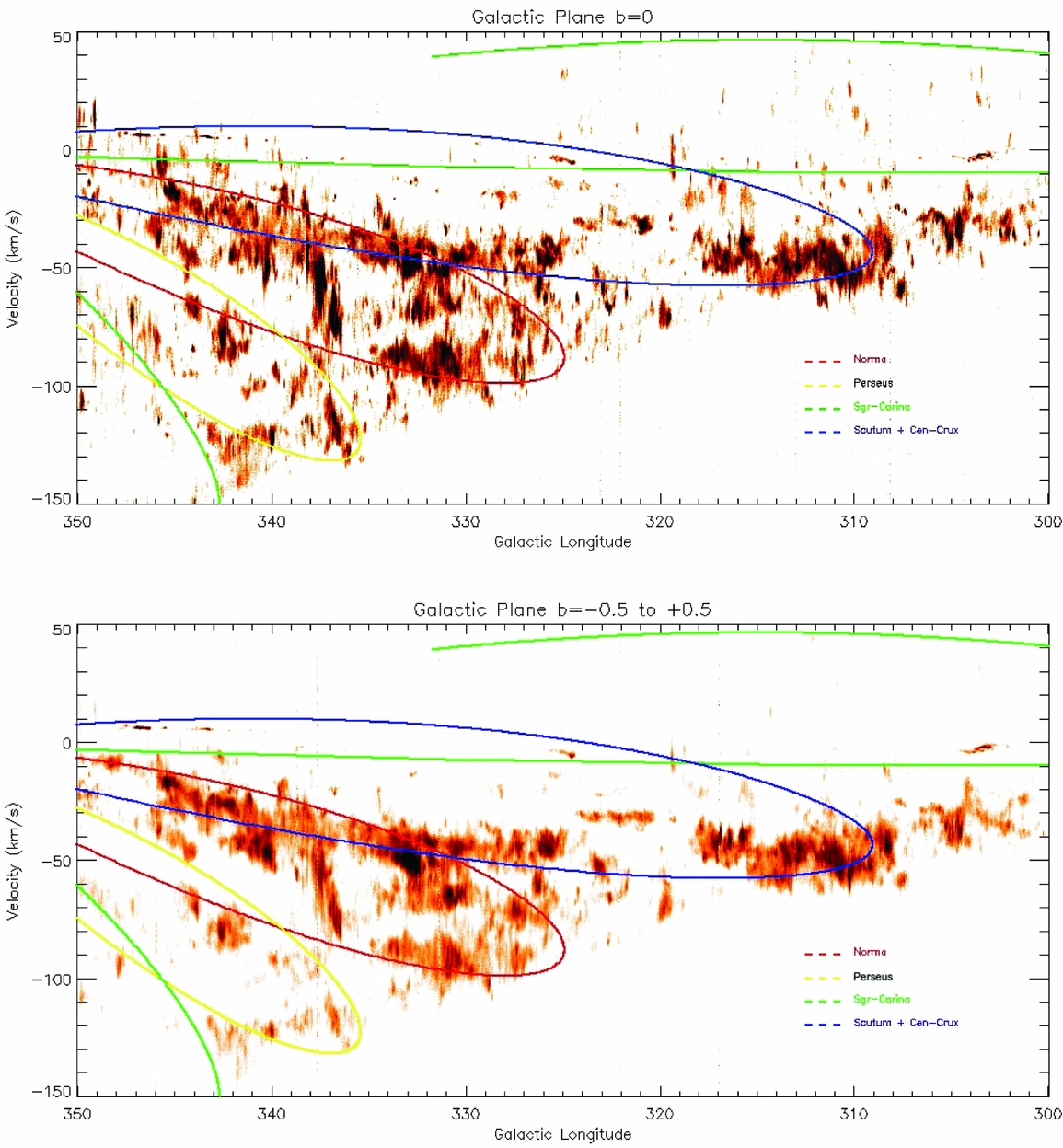
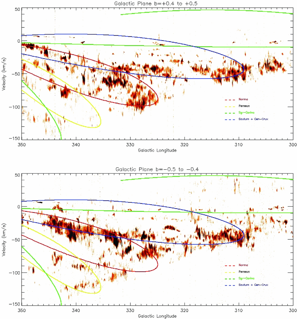
Figures 5 and 6 show PV slices of the CO emission averaged over four different ranges in latitude overlaid with the positions of four spiral arms from the Galaxy model of Vallée (Reference Vallée2016), i.e. a pitch angle of 13.1°, central bar length of 2.2 kpc inclined at −30° to our sightline, Galactic Centre distance of 8.0 kpc, and a flat rotation curve with velocity 220 km s−1. Figure 5 shows the central plane |b| < ±0.05° and the entire data range of |b| < ±0.5°, while Figure 6 shows the very top (b = +0.4 to +0.5°) and bottom (b = −0.5 to −0.4°) of the surveyed field. The spiral arm model and its associated distance–velocity relationship are shown in Figure 7.
12CO position-velocity plots as a function of Galactic longitude. l is on the x-axis, V LSR (the radial velocity) in km s−1 is on the y-axis. The data has been averaged between latitudes b = −0.05° and +0.05° (top) and b = −0.5° to +0.5 (bottom), respectively representing the midpoint of the plane and the entire surveyed plane. The solid lines are the model positions for the centres of the four spiral arms in the model of Vallée (Reference Vallée2016). Note also that some artefacts are visible as features extending across the entire velocity direction, resulting from residual systematic effects.
12CO position-velocity plots as a function of Galactic longitude, l, on the x-axis and the radial velocity, V LSR, in km s−1 on the y-axis. The data has been averaged between latitudes b = +0.5° and +0.4° (top) and b = −0.5° to −0.4° (bottom), representing the top and the bottom of the surveyed plane. The solid lines are the model positions for the centres of the four spiral arms in the model of Vallée (Reference Vallée2016). Note also that some artefacts of residual systematic effects are visible as features extending across the entire velocity direction.
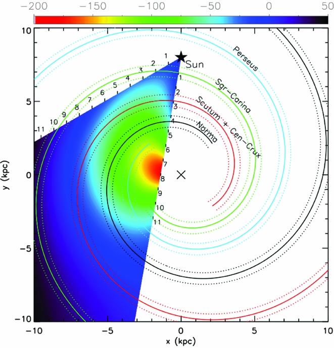
A schematic of the four spiral arms of the Milky Way Galaxy. Arm names, the Galactic centre, and the location of the Sun are indicated. A colour-scale displays the expected kinematic line-of-sight velocity from the reference point of the Sun. The Galaxy is modelled as having a pitch angle of 13.1°, a central bar length of 2.2 kpc inclined at −30° to our sightline, a Galactic centre distance of 8.0 kpc and a flat rotation curve with velocity 220 km s−1 (Vallée Reference Vallée2016).
The observed features generally correspond to giant molecular cloud complexes within the spiral arms, with their velocity widths corresponding to internal motions within the complexes rather than the differential distances that could be inferred by applying a Galactic rotation model. In a few instances, prominent outflows are evident as molecular emission that is quite extended in velocity but narrow in the longitudinal direction; these could also be giant molecular clouds at far Galactic distances, but such clouds are generally expected to be somewhat extended in longitude.
However, while the molecular gas does tend to follow the trajectory of the spiral arm model in Figure 7, the detailed agreement is only modest. The differences between the PV-plots for the different latitude ranges are also striking, showing how discrete molecular gas is even within the Galactic Plane. Little 12CO(1–0) emission is evident at ‘forbidden’ velocities, i.e. those that are more negative than the tangent point velocity at each latitude, and in particular the most negative velocities for each of the four model spiral arm positions.
Figure 8 shows the distribution of molecular mass with Galactic longitude, averaged for each square degree of the survey range. This calculation is as in Braiding et al. (Reference Braiding2015) for l = 320–330°, now extended to l = 300–350° and covering the entirety of DR3: Applying the CO X-factor to convert 12CO flux to column density using a conversion factor of 2.7 × 1020cm−2 (K km s−1)−1, the value derived for |b| < 1° in Dame et al. (Reference Dame, Hartmann and Thaddeus2001). Though larger than the 1.8 × 1020cm−2 commonly used for |b| < 5°, it is within the uncertainties discussed by Bolatto, Wolfire, & Leroy (Reference Bolatto, Wolfire and Leroy2013) in their meta-analysis of X-factor values derived from a variety of observational and theoretical studies. The mass is calculated from the column density by applying a Galactic rotation curve to convert velocity to distance. This included making assumptions regarding whether gas velocities relate to near- or far-side distances. Comparison with the spiral arm positions suggest that the bulk of the gas observed does arise at near distances, similar to the assumption in Braiding et al. (Reference Braiding2015). However, we now present mass estimates based on the two extremes, of all the gas being at the near-distance and all at the far-distance. We have not included, however, molecular gas at positive velocities, which lie beyond the Solar Circle in this calculation. While such gas is clearly present at some PV-plot positions, the low fluxes when averaged over an entire degree, combined with their large distances, result in large absolute errors in the mass determination. Hence, we have not included them in Figure 8 (but see also the note at the end of the next paragraph). We find that typically there are a few× 106 M⊙ of molecular gas per square degree from l = 300° to l = 330°. The mass then rises to a peak of around 107 M⊙ per square degree between l = 330° and 340°, before falling by a factor of 2 at l = 350°. The total molecular gas within ±0.5° of the Galactic Plane, in the 50° from l = 300–350°, is found to be ~2 × 10⁸ M⊙ (if all were at the near distance) and ~9 × 10⁸ M⊙ (all at the far distance). While not included in the plot, the total amount of gas lying beyond the solar circle is estimated to be around 4 × 10⁷ M⊙. This would contribute an additional 5 to 20% to the total molecular gas content calculated here. From the moment maps in Appendix A.4, it is clear that we have observed not only 12CO, but also 13CO at far distances with velocities >+30 km s−1.
Molecular mass distribution for the inner degree of latitude across the Galaxy, extending from l = 300–350°. Masses are calculated using a 12CO X-factor of 2.7× 1020cm−2 (K km s−1)−1 to convert line fluxes to column densities for all gas detected within the solar circle (i.e. that with negative velocities). The solid line illustrates the mass calculated using the assumption of near-side distances, the dotted line assumes far-side distances (and is divided by a factor of 10 for presentation).

4.3. C18O clump catalogue
When the faint C18O line is detected, it is almost certainly optically thin due to the low abundance of the molecule with respect to 12CO, and so provides a sightline that penetrates entirely through clouds. Thus, the highest column density molecular clumps are detected in C18O. In order to investigate the distribution of C18O clumps across the Milky Way, we isolate individual clumps by applying the ClumpfindFootnote 4 algorithm (Williams, de Geus, & Blitz Reference Williams, de Geus and Blitz1994) to the region between 330 < l < 340° where −0.5 < b < +0.5, and −140 < V LSR < +50 km s−1. In order to efficiently run this calculation on the Mopra CO data cubes, a number of simplifications needed to be performed: First, the data was binned by 10 spectral channels (reducing the velocity resolution to ~0.92 km s−1) and second, it was box smoothed using the IDL routine smoothFootnote 5. The relative 1σ emission level of the C18O data cube is then ~0.10 K (derived by computing the standard deviation of the spectra in an emission-free region).
Clumpfind operates by finding local peaks of emission and then contouring around them to decompose the data cube into a set of clumps of C18O emission. It requires two input parameters to work: the increment between contour levels, inc, and the desired lower limit of clump emission, low; after a series of tests, both of these were assigned the value of 0.45 K, equivalent to the 4.5σ emission level.
The resulting bright C18O clumps are presented in Table 3 of Appendix A.5; for each of these, we report the coordinates of the clump centroid, the average and peak main beam brightness temperature, the relative FWHM extensions in arcsec and km s−1, and its radius in arcseconds. Prior to computing the physical properties of each clump, we compare the C18O and 13CO spectral profiles for each line of sight, rejecting those false detections that are noisy spikes in the C18O band without a clear peak in both CO isotopologues. We also check the clumpfind ID assignation to ensure each clump is physically distinct (as it lists nearby local maxima within the same physical structure as independent clumps); within the catalogue, the minimum separation between two centroids is nine voxels.
Using the model described above in Section 4.2, we calculate near and far distances to each clump, which are also listed in Table 3. Following Wilson, Rohlfs, & Hüttemeister (Reference Wilson, Rohlfs and Hüttemeister2009), we derive the C18O column density for each clump, assuming that the gas is in local thermodynamic equilibrium (LTE) at a fixed T ex = 10 K, to be
 $$\begin{equation}
\centering N(\mathrm{C^{18}O})= 3.0\times 10^{14}\frac{T_\mathrm{ex}}{1-e^{-(T_{0}^{18}/T_\mathrm{ex})}}\int {\tau _{18}\text{d}{v} },
\end{equation}$$
$$\begin{equation}
\centering N(\mathrm{C^{18}O})= 3.0\times 10^{14}\frac{T_\mathrm{ex}}{1-e^{-(T_{0}^{18}/T_\mathrm{ex})}}\int {\tau _{18}\text{d}{v} },
\end{equation}$$
where T 180 = 5.27 K is the energy level of the J = 1–0 C18O transition, and dv is the velocity interval in km s−1. The optical depth, τ18, is
 $$\begin{equation}
\tau _{18} = -\ln \biggr (1-\frac{T^{18}_{\rm MB}}{5.27}\biggr [\big [e^{5.27/T_{\rm ex}} -1\big ]^{-1}-0.16\biggr ]^{-1}\biggr ).
\end{equation}$$
$$\begin{equation}
\tau _{18} = -\ln \biggr (1-\frac{T^{18}_{\rm MB}}{5.27}\biggr [\big [e^{5.27/T_{\rm ex}} -1\big ]^{-1}-0.16\biggr ]^{-1}\biggr ).
\end{equation}$$
The column density of H2, N(H2) is then calculated for each clump using the abundance ratio of [H2/C18O]=5.88 × 106 from Frerking, Langer, & Wilson (Reference Frerking, Langer and Wilson1982). Finally, we are able to derive near and far masses for each clump. Assuming that the clumps are all located at the near distance, the total mass traced by C18O in this region is ~2.5 × 10⁶ M⊙, equivalent to 10% of the total molecular gas mass traced by 12CO in the same portion of Galactic Plane, as only the highest density regions are traced by C18O. Nevertheless, the C18O molecule provides an important optically thin tracer of the molecular gas.
5 ISM SURVEY SYNERGIES
The Mopra CO survey is a timely addition to several Galactic Plane surveys currently under way. In particular, we have observed to a Galactic longitude of l = 11°, giving 2 deg2 of overlap with the Northern Hemisphere FOREST Unbiased Galactic plane Imaging survey with the Nobeyama 45-m telescope (FUGIN; Minamidani et al. Reference Minamidani2015; Umemoto et al. Reference Umemoto2017), a similarly high resolution 12CO(1–0) survey covering from l = 10–50° and l = 198–236°, where |b| < 1°. Preliminary work comparing these surveys is now underway, but as mentioned in Section 4, similar comparisons with the Nanten2 CO survey suggest that the observed fluxes and structures in the overlapping region will be equivalent (H. Sano, 2017, private communication).
Combining Mopra CO with data from other surveys presents the opportunity to fully characterise regions of interest in order to probe the origins and history of molecular clouds (Burton et al. Reference Burton2013). Recently, Sano et al. (Reference Sano2017b) presented work using data from this survey, ASTE and Nanten2 to investigate high-mass star cluster formation triggered by cloud–cloud collisions, in particular focusing on the H ii region RCW 36, located in the Vela Molecular Ridge. They suggested that a cloud–cloud collision formed RCW 36 and its stellar cluster, with a relative velocity separation of ~5 km s−1. The estimated cloud separation of ~0.85 pc was estimated to occur over a time-scale of ~0.2 Myr, assuming a distance of 1.9 kpc, consistent with the age of the cluster. The resulting O-type star formation lead to a high measured CO rotational temperature.
CO isotopologue data from DR1 of the Mopra Galactic Plane survey was exploited in an investigation of the so-called ‘dark’ component of molecular gas towards a cold, filamentary molecular cloud in the G328 sight-line (Burton et al. Reference Burton2014, Reference Burton2015). The authors compared the distribution of atomic H i-traced gas to atomic C emission (which traces some CO-dark molecular gas) and the CO-traced molecules observed in DR1. They found that 13CO and [C i] show similar distributions and velocity profiles, the abundance of atomic C increases towards the molecular cloud edges, consistent with CO photodissociation by an average interstellar radiation field and CR ionisation at low optical depths. Further comparison to dust images from Herschel showed that the cloud was IR-dark and that no star formation is yet occurring within the young filament. Extended studies using C+ observations from the Stratospheric Observatory for Infrared Astronomy (SOFIA) will target gas that may be in the transition phase between atomic and molecular forms of Carbon (Risacher et al. Reference Risacher2016), allowing a better tracing of the dark molecular gas that has been inferred from gamma-ray observations (see Section 6) and to study molecular cloud formation in detail.
The APEX Telescope Large Area Survey of the Galaxy (ATLASGAL) has been used to perform an unbiased census of massive dense clumps in the Galactic Plane at 870 μm, using Mopra CO data to provide radial velocities to ~500 of the clumps (Urquhart et al. Reference Urquhart2018). The properties of these clumps were exploited to develop an evolutionary classification scheme showing trends for increasing dust temperatures and luminosities as a function of evolution, showing that most of the clumps are already associated with star formation. We expect to determine a similar evolutionary scheme for molecular cloud cores (including the C18O cores presented in Section 4.3), using the Mopra CO and other survey data in future.
The OH λ = 18 cm lines are complementary to CO and H i when estimating the mass of H2 in molecular clouds, as at densities well below 103 cm−3 CO is affected by ultraviolet shielding, interstellar chemistry, and sub-thermal processes (Dickey et al. Reference Dickey2013). The GASKAP (The Galactic Australian Square Kilometre Array Pathfinder) survey will trace atomic hydrogen directly through the H i transition and OH (Dickey et al. Reference Dickey2013). The GASKAP survey will achieve spatial resolutions of 20–60 arcsec for H i and 90–180 arcsec for OH, the former comparable with the Mopra CO survey, allowing astronomers to carry out pixel to pixel comparisons between the different tracers. Also using ASKAP, the EMU (Evolutionary Map of the Universe) survey will provide a similar-resolution high sensitivity map of radio continuum emission in the Galactic Plane, allowing the detection of H ii regions, supernova remnants and planetary nebulae at similar resolutions to Mopra CO and GASKAP (Norris et al. Reference Norris2011). Future improvements to the velocity resolution of ASKAP may bring it closer to that of Mopra.
Towards a better understanding of the motions of the Galactic centre, Yan et al. (Reference Yan2017) employed Mopra 12CO and 13CO data in conjunction with OH absorption data from the Southern Parkes Large-Area Survey in Hydroxyl (SPLASH; Dawson et al. Reference Dawson2014) to create a three-dimensional image of the Galactic centre region at a spatial resolution of 38 pc. The Galactic centre was well-described with a bar-like structure at an angle of 67 ± 2° to the line of sight. More generally, the Mopra CO data from the CMZ (Blackwell et al. in preparation) will be key to studies of the star formation and its effect on the evolution of the CMZ (e.g. Kruijssen et al. Reference Kruijssen, Dale and Longmore2015).
Interstellar medium surveys are critical to X-ray and other high-energy studies, where they are used to determine distances to supernova remnants, particularly using morphology anti-correlations and photoelectric absorption studies (e.g. Maxted et al. Reference Maxted2018). Heinz et al. (Reference Heinz2015) observed X-ray light echoes from the X-ray binary Circinus X-1, which demonstrated four well-defined rings with radii from 5 to 13 arcmin. By modelling the dust distribution towards Circinus X-1 and comparing that to 12CO emission from Data Release 3, they were able to identify the source clouds for the innermost rings and determine the distance to Circinus X-1 to be ~9.4 kpc for the binary system, ruling out previous near distance estimates of ~4 kpc.
The Mopra CO survey will also be well-complemented by 13CO(2–1) data from SEDIGISM (Structure, Excitation, and Dynamics of the Inner Galactic Interstellar Medium; Schuller et al. Reference Schuller2017), allowing the calculation of rotational temperature estimates for regions that are optically thick in 12CO and 13CO(1–0). Similarly, James Clerk Maxwell Telescope (JCMT) 12CO(3–2) observations (Dempsey, Thomas, & Currie Reference Dempsey, Thomas and Currie2013) will be used to refine temperature and column density estimations for molecular clouds of interest.
Perhaps most importantly, the Mopra CO survey data will be used as a finder chart for objects of interest to be observed with ALMA, which offers arcsecond-level spatial resolution in the CO(1–0) transition (Mathews et al. Reference Mathews2013). We note that Mopra CO data has guided successful ALMA and SOFIA applications for observations towards molecular cores interacting with the young supernova remnant, RX J1713.7−3946 (Rowell Reference Rowell2017; Sano Reference Sano2017a). The resultant data will reveal the extremely fine details of these structures and provide an important step towards understanding CR origins.
Future ISM catalogues of sources of interest traced by the Mopra CO survey will be essential for determining the best objects to follow-up with ALMA. A sample catalogue of bright C18O clumps is in Appendix A.5, along with characterisations of the location, size, temperature, and mass. The complete catalogue will provide supplementary information useful for targeting dense clumps in the star-formation research.
6 GAMMA-RAY OBSERVATIONS
Gamma-ray maps provide an important window into the gas distribution of the Galaxy that rely on studies of CO, [C i], [C ii], and H i. A large component of gamma-ray emission from the Milky Way comes from three distinct so-called ‘diffuse’ source types (see e.g. Acero et al. Reference Acero2013, Reference Acero2017; Dubus et al. Reference Dubus2013):
1. Truly diffuse gamma-rays from CRs circulating in the Galactic Plane for ≳ 106 yr, i.e. the diffuse CR ‘sea’.
2. Local gamma-ray enhancements from CRs escaping local accelerators on time-frames ≲ 105 yr.
3. Unresolved sources of gamma-ray emission across the Galaxy.
Diffuse sources of type (1) and (2) involve CR protons interacting with gas in the Galactic Plane via proton–proton collisions that produce charged and neutral pions. The neutral pions quickly decay into gamma-ray photons. Diffuse sources of type (3) may also have a component of gamma-ray emission produced via this mechanism, depending on the source.
Unlike spectral line emission, gamma-rays from pion-decay can be considered a general tracer of gas density independent of temperature or chemistry. As the gamma-ray flux generated by proton–proton interactions is a product of CR density and gas density, gamma-ray maps can be used to highlight excesses of both gas and CRs. It follows that gas studies and gamma-ray astronomy are intimately tied together.
In order to identify gamma-ray sources in the Galactic Plane maps from Fermi-LAT, which operates in the 0.02–300 GeV gamma-ray regime (Atwood et al. Reference Atwood2009), a model of the gamma-ray emission from diffuse source (1) was required. This model was constructed from H i and CO gas maps of similar resolution (e.g. McClure-Griffiths et al. Reference McClure-Griffiths, Dickey, Gaensler, Green, Haverkorn and Strasser2005; Dame et al. Reference Dame, Hartmann and Thaddeus2001) and revealed that previous work underestimated the gamma-ray Galactic contribution at high latitudes and hence overestimated the background CR ‘sea’ (e.g. Strong, Moskalenko, & Reimer Reference Strong, Moskalenko and Reimer2004).
Galactic molecular cores resolved at sub-arcminute scales in both gamma-rays and CO(1–0) emission will enable the identification of pion-decay signatures near CR sources (Cameron Reference Cameron2012; Acharya et al. Reference Acharya2013), and may deliver kinematic distance solutions for CR sources (Cherenkov Telescope Array Consortium et al. 2017). The signature of this decay will be particularly strong if the gamma-ray spectral index is altered by CR diffusion into molecular cores due to energy-dependent propagation (e.g. Gabici, Aharonian, & Blasi Reference Gabici, Aharonian and Blasi2007; Maxted et al. Reference Maxted2012). Indeed, a common theme developing for young gamma-ray shell-type supernova remnants (which are regarded as key PeV CR acceleration candidates) is the existence of sub-arcminute-scale molecular cores embedded in the perimeter of regions blown out by the progenitor star (Fukui Reference Fukui, Aharonian, Hofmann and Rieger2008; Moriguchi et al. Reference Moriguchi, Tamura, Tawara, Sasago, Yamaoka, Onishi and Fukui2005; Sano et al. Reference Sano2013; Maxted et al. Reference Maxted2013; Fukuda et al. Reference Fukuda, Yoshiike, Sano, Torii, Yamamoto, Acero and Fukui2014; Kavanagh et al. Reference Kavanagh, Sasaki, Bozzetto, Filipović, Points, Maggi and Haberl2015; Fukui et al. Reference Fukui2017; Sano et al. Reference Sano2017c). The next-generation CTA (Cherenkov Telescope Array Consortium et al. 2017) is expected to provide gamma-ray maps at a resolution sufficient to identify local peaks due to cloud clumps and filaments. Furthermore, the Mopra CO survey will probe interstellar medium dynamics by revealing broad-line or asymmetric emission indicative of the shock-gas interactions, as is expected of some gamma-ray sources like older supernova shocks and pulsar wind nebulae (e.g. Arikawa et al. Reference Arikawa, Tatematsu, Sekimoto and Takahashi1999).
Data from the Mopra Galactic Plane CO Survey have already been used to examine the nature of gamma-ray sources observed with the highest resolution gamma-ray telescope, HESS (High Energy Stereoscopic System, Aharonian et al. Reference Aharonian2006). Understanding the links between TeV gamma-ray emission and the parent high-energy particle populations local to extreme Galactic objects is a step forward in the search for elusive CR hadron acceleration sites; pulsar wind nebulae and SNRs with associated gamma-ray detections are the primary candidates in the pursuit for Galactic CR sources.
Lau et al. (Reference Lau2017b) exploited Mopra CO and CS isotopologue data to investigate the gamma-ray sources HESS J1640−465 and HESS J1641−463, which are positionally coincident with the SNRs G338.3−0.0 and G338.5+0.1. The authors found coincident diffuse molecular gas, with a bright complex of dense gas and H ii regions connecting the SNRs. CO-derived masses were then utilised to estimate the density of >1TeV CRs assuming that the gamma-ray emission was caused by pion-decay following proton-proton interactions. The values inferred were in the range of 100–1 000 times the Solar value (Lau et al. Reference Lau2017b). Similarly, CO and CS observations that identify filamentary molecular features towards the unidentified objects HESS J1614−518 and HESS J1616−508 (Lau et al. Reference Lau2017a) represent the first steps in forming an understanding of the nature of gamma-ray emitters.
Maxted et al. (Reference Maxted2018) compared line of sight column densities from Mopra CO and the SGPS H i emission to X-ray absorption column densities for the bright shell-type gamma-ray SNR, HESS J1731−347. This enabled the calculation of a kinematic distance to the source, and revealed a large associated molecular gas cloud that bridged the region between HESS J1731−347 and a nearby unidentified gamma-ray source, HESS J1729−345. Such a discovery adds weight to the suggestion that some unidentified gamma-ray sources are the product of so-called ‘runaway CRs’ that escape a CR acceleration site and diffuse into nearby molecular gas clouds (i.e. diffuse sources of type 2). Similar CR scenarios have also been investigated for pulsar wind nebulae and their progenitor supernova remnants (e.g. HESS J1826−130, Voisin et al. Reference Voisin, Rowell, Burton, Walsh, Fukui and Aharonian2016).
With the CTA now under construction (Cherenkov Telescope Array Consortium et al. 2017), subarcminute resolution gamma-ray maps will soon become available. As with Fermi-LAT, CTA will require similar-resolution gas maps to characterise the diffuse gamma-ray emission components (1 and 2) and enable studies of gamma-ray sources and dark gas. Furthermore, CTA’s improved sensitivity will enable it to detect sources across the Galactic disk, expanding on the rather limited (few kpc for sources of <10% Crab flux) horizon achieved by current telescopes like HESS. Towards this future, we are preparing molecular gas maps that will fully parametrise Mopra CO, FUGIN, and GASKAP data for use in gamma-ray modelling of the Galactic Plane (e.g. using GALPROP, PICARD and DRAGON; Strong & Moskalenko Reference Strong and Moskalenko1998; Kissmann Reference Kissmann2014; Evoli et al. Reference Evoli, Gaggero, Vittino, Di Bernardo, Di Mauro, Ligorini, Ullio and Grasso2017, respectively).
7 SUMMARY
We present the third data release of the Mopra Southern Galactic Plane CO survey, covering 50 deg2 between Galactic longitude l = 300–350° and latitude b = ±0.5°. These data are part of a larger campaign to map the molecular gas of the inner Galactic Plane in 12CO, 13CO, C18O, and C17O(1–0) emission.
We find general agreement between the CO spectral line profiles of the Mopra survey and those of the Columbia survey for each square degree of coverage. Furthermore, we find a modest agreement between the Mopra survey PV structure and a recent Galactic Plane model (Vallée Reference Vallée2016). A preliminary catalogue of C18O clumps presented traces ~10% of the observed 12CO molecular gas, illustrating the importance of this optically thin tracer of molecular gas.
The Mopra CO survey, which is estimated to trace a ~few× 106 M⊙ of molecular gas per square degree, is already making an impact on the search for Galactic CR sources and star formation research. We discuss past and future multi-wavelength investigations towards a number of Galactic Plane sources and synergies with other surveys.
The Mopra CO survey is still ongoing, with the intention of covering the entire fourth quadrant and expanding to Galactic latitudes beyond b = ±1.0° by the end of 2018. As the data are published, they are being made available at the survey website, and the PASA data archive.
ACKNOWLEDGEMENTS
The Mopra radio telescope is part of the Australia Telescope National Facility. Operations support was provided by the University of New South Wales, the University of Adelaide, and Western Sydney University. Many staff of the ATNF have contributed to the success of the remote operations at Mopra. We particularly wish to acknowledge the contributions of David Brodrick, Philip Edwards, Brett Hiscock, and Peter Mirtschin.
This research made use of Astropy, a community-developed core Python package for Astronomy (Astropy Collaboration et al. 2013) and the IDL Astronomy Library (Landsman Reference Landsman, Hanisch, Brissenden and Barnes1993).
We are indebted also to the financial support of the #TeamMopra kickstarter contributors, listed at www.mopra.org. The University of New South Wales Digital Filter Bank used for the observations with the Mopra Telescope (the UNSW–MOPS) was provided with support from the Australian Research Council (ARC). We also acknowledge ARC support through Discovery Project DP120101585 and Linkage, Infrastructure, Equipment, and Facilities project LE160100094.
SUPPLEMENTARY MATERIAL
To view supplementary material for this article, please visit https://doi.org/10.1017/pasa.2018.18.


