


Highlights
What is already known?
-
• Network meta-analysis (NMA) has limitations for synthesizing evidence across multiple treatment doses and timepoints, which can lead to disconnected treatment networks, when available data are discarded, or treatment nodes are pooled.
-
• Model-based network meta-analysis (MBNMA) has been developed to synthesize information across either multiple dose levels or multiple timepoints.
What is new?
-
• We extend the MBNMA framework to a joint dose–response and time–course MBNMA (DT-MBNMA), combining the strengths of DT-MBNMA.
-
• We use both simulations and a network of studies in obesity, to demonstrate how DT-MBNMA seamlessly integrates phase 2 and phase 3 data in NMA and provides greater precision on the indirect treatment effects, as compared to standard NMA.
Potential impact for RSM readers
-
• Phase 2 dose-finding studies can offer valuable information for health technology assessment (HTA), because the studies often include an active comparator, but their inclusion in standard evidence synthesis is often hampered by shorter follow-up and/or investigational doses.
-
• DT-MBNMA provides comprehensive integration of data generated across a drug development program, with applications to inform trial designs and HTA .
1 Introduction
Network meta-analysis (NMA) plays a crucial role in health technology assessment (HTA) by providing methods to compare multiple interventions simultaneously when direct head-to-head comparisons between all interventions are not available from individual randomized clinical trials (RCTs). NMA respects randomization and combines relative treatment effects, estimating heterogeneity between studies and is able to provide comparison between any two treatments in a connected network. However, the NMA framework has limitations in synthesizing evidence across multiple treatment doses and timepoints, which can lead to disconnected networks.Reference Pedder, Dias, Bennetts, Boucher and Welton 1
Model-based meta-analysis (MBMA) is a recent method that addresses some of these limitations by handling complex dose–response and time–course relationships constructed from RCTs in the form of aggregate data.Reference Chan, Peskov and Song 2 The approach centres around modelling of arm-level results (i.e., absolute effects). In MBMA, aggregated data from individual studies are integrated into a single statistical model, which allows for the estimation of placebo, drug response, and assessment of heterogeneity across arm-level results. However, this approach models absolute outcomes in each trial arm rather than within-trial treatment contrasts, thereby foregoing the protection against confounding that randomization provides for estimation of treatment effects.
Recently, model-based network meta-analysis (MBNMA) has been proposed to combine both approaches,Reference Pedder, Dias, Bennetts, Boucher and Welton 3 respecting randomization while borrowing strength across multiple dose levels of treatments or timepoints. Pedder et al.Reference Pedder, Dias, Bennetts, Boucher and Welton 3 developed time–course MBNMA to model treatment effects over time, treating each treatment (or dose) as a discrete entity. Separately, Mawdsley et al.Reference Mawdsley, Bennetts, Dias, Boucher and Welton 4 developed dose–response MBNMA to model continuous dose–response relationships at single timepoints. Our framework extends these approaches by jointly modelling both dimensions, allowing structural parameters of time–course functions to themselves be functions of dose. The framework allows for combining data at multiple timepoints from studies in early clinical development with a broad range of doses to late-stage clinical studies with a limited range of doses. This may increase statistical efficiency by borrowing strengths from the full dose–response profile.Reference Pedder, Dias, Bennetts, Boucher and Welton 1 The dose–response and time–course MBNMA (DT-MBNMA) framework reduces to time–course MBNMA (T-MBNMA) when dose is modelled as discrete treatment effects and to dose–response MBNMA when analysing a single timepoint.
Borrowing strength across multiple studies in this way has applications in HTA, where careful integration of phase 2 dose-finding studies can provide valuable additional evidence. Phase 2 studies often include active comparators and broader dose ranges, but have shorter treatment durations than phase 3. The DT-MBNMA framework accounts for these differences in treatment duration and dose selection, enabling evidence synthesis across development phases. We follow the MBNMA literature and focus on the typical situation in HTA where only aggregate summary data are available. Beyond HTA, the framework’s ability to predict both relative and absolute effects at any dose and timepoint also makes it a useful tool for decision-making and planning within pharmaceutical companies.
We illustrate the DT-MBNMA framework with an application in obesity. Obesity is a chronic disease with high prevalence and associated comorbidities, making it a growing global health concern. Comorbidities, such as type 2 diabetes, hypertension, ventilatory dysfunction, arthrosis, venous and lymphatic circulation diseases, and depression underscore the wide-ranging health implications of obesity, resulting in increased morbidity and mortality.Reference Abdelaal, le Roux and Docherty 5 Here, the treatment duration required for the stabilization of weight loss profile is long and therefore early clinical development (e.g., dose-finding studies) does not explore the full treatment potential of a given dose.Reference Astrup, Rossner and Van Gaal 6
The DT-MBNMA framework is first evaluated in a simulation study, where the true values and model structure are known and then second applied to a network of RCTs in the therapeutic area of obesity disease. We end with a discussion of the framework in the context of guiding future study designs and supporting clinical decision-making.
2 Methods
2.1 Overview of modelling
The DT-MBNMA framework addresses how treatment effects evolve over time and vary across doses by combining three components:
-
1. Response model (Section 2.2): The model uses aggregate data extracted from publications (means and standard errors [SEs] at each timepoint for each study arm). These summaries are assumed to follow a multivariate normal distribution, with expected values come from parametric functions describing time–course and dose–response (Table 1). SEs are treated as known, extracted from publications while correlations are either set to zero, estimated using simple time series models, or uses observed correlations.
-
2. Parameter model (Section 2.3): The model estimates structural parameters that govern response functions rather than separate effects for each dose-timepoint combination. Response functions are defined based on subject-matter knowledge. For example, a time–course might be characterized by maximum effect and rate of onset; dose–response by maximum effect and the dose producing half-maximal response. These parameters vary across studies through study-specific reference levels (fixed effects) and treatment-specific deviations (random effects). Dose-–response functions map dose levels to relative effects, enabling information sharing across doses, timepoints, and trials.
-
3. Random effects specification and diagnostics (Section 2.4): Between-study variability in treatment effects is handled through random effects with a covariance matrix that allows parameters to correlate (e.g., treatments differing in maximum effect may also differ in time-to-effect). Multi-arm trials receive special handling to account for correlation between arms sharing a common reference. This random effects structure provides diagnostics: large between-study variability suggests model misspecification or network inconsistency.
Response functions for joint time–course and dose–response modelling

Table 1. Long description
The table has five rows and five columns. The columns are Model, Function f dot, Parameters, Time-course, and Dose-response. Row one is Log-linear with function b times log open parenthesis x plus one close parenthesis, parameter normal prior on b, and x in Dose-response. Row two is Linear with function b times x, parameter normal prior on b, and x in Dose-response. Row three is E max with function E max times x all over exp open parenthesis x sub 50 close parenthesis plus x, parameters normal priors on E max and log x sub 50, and x in both Time-course and Dose-response. Row four is Exponential with function E max times open parenthesis one minus exp open parenthesis minus exp open parenthesis k T close parenthesis times x close parenthesis close parenthesis, parameters E max and log k T, and x in Time-course. Row five is Bateman with function A times open parenthesis exp open parenthesis k T sub one close parenthesis all over exp open parenthesis k T sub one close parenthesis minus exp open parenthesis k T sub two close parenthesis close parenthesis times open parenthesis exp open parenthesis minus exp open parenthesis k T sub two close parenthesis times x minus exp open parenthesis k T sub one close parenthesis times x close parenthesis close parenthesis, parameters A, log k T sub two, and log k T sub one, and x in Time-course. The note states that x denotes function explored for modeling time-course, dose-response, or both.
Note: The mark ‘x’ denotes function that explored for modelling time–course, dose–response or both.
The framework nests simpler approaches: replacing parametric dose–response with discrete treatment effects yields T-MBNMA; using only end-of-treatment timepoints yields standard NMA. This nested conceptualization allows assessment of whether added complexity improves evidence synthesis.
2.2 Response model
We consider the typical setting where only aggregate-level trial data are available from publications or trial reports. Let y ij denote a vector of summary statistics for study (i = 1 ,…, k) and arm (j = 1 ,…, ni) across the time–course profile (t = [0 ,…, τij]) with dimension (ni x (τij+1)). Here ni denotes the number of arms in study i, and τij denotes the end-of-treatment timepoint in study i and treatment arm j. Our framework applies to outcomes measured repeatedly at protocol-defined timepoints where time–course relationships are biologically plausible. Repeated observations on the individual are correlated over time and therefore it is reasonable to specify a multivariate normal likelihood for the aggregate data:

where μ ij is the vector of modelled outcomes generated from the response functions in Table 1, which are motivated in Section 2.2 of the article. The covariance matrix is denoted by ∑ ij. If the clinical outcome is given in absolute values, then an intercept should be added to the equations in Table 1, addressing the outcome at time = 0.
The diagonal elements in ∑ ij are the within-arm variances (se 2 ij), and in line with standard NMA, are assumed known. The within-arm SEs can be extracted or digitized from publications, whereas within-arm correlations seldom are reported. Therefore, we follow the approach of Pedder et al.Reference Pedder, Dias, Bennetts, Boucher and Welton 3 by either setting within-arm correlations to zero (i.e., a univariate normal likelihood) or estimating within-arm correlations based on the aggregate response summaries. Based on the work of Pedder et al.,Reference Pedder, Dias, Bennetts, Boucher and Welton 3 an autoregressive of first order structure (AR-1) appears reasonable because covariances are dependent on the time distance between clinical visits. In this article, data are simulated at the individual patient level (IPD). In the illustrative dataset, IPD is available to investigate the consequence of ignoring or approximating the within-arm correlation structure because correlations estimated from IPD will be at the individual level, which may be different to summary-level correlations.
2.3 Parameter model
In statistical terms, a random effects DT-MBNMA is a nonlinear mixed effect (NLME) model. NLME models are widely used in pharmacometrics, particularly for characterizing the time–course of drug concentrations and their effects on the body. The variation within and between studies is modelled through the structural parameters (e.g., time-constant (kT) or maximum effect (E
maxT) for the exponential function) of the response functions in Table 1, which are presented in detail in Section 2.4. To generalize, the model for the p’th structural parameter (
${\theta}_{ij}^{(p)}$
 ) can be written as

where g(.) is a link function, e.g., the time-constants are log transformed, ensuring that they are positive real numbers on the time scale. The
${\mu}_i^{(p)}$
 is the study-specific level for the reference treatment in the ith study, which is treated as a fixed effect and can be viewed as a nuisance parameter. The function f(.) is a parametric dose–response function and commonly used response functions are presented in Section 2.2 of the article. The response function f(.) maps the treatment doses to relative treatment effects and
${\mathbf{X}}_{\boldsymbol{ij}}$
is the study-specific level for the reference treatment in the ith study, which is treated as a fixed effect and can be viewed as a nuisance parameter. The function f(.) is a parametric dose–response function and commonly used response functions are presented in Section 2.2 of the article. The response function f(.) maps the treatment doses to relative treatment effects and
${\mathbf{X}}_{\boldsymbol{ij}}$
 is a design matrix, encoding agent specific effects, and
${\boldsymbol{\unicode{x3b2}}}^{(p)}$
is a design matrix, encoding agent specific effects, and
${\boldsymbol{\unicode{x3b2}}}^{(p)}$
 is a vector of agent specific dose–response parameters (e.g., median effective dose (ED50) and maximum effect (E
maxD)). The proposed framework has the flexibility to model time–course profiles that are dose-dependent.
is a vector of agent specific dose–response parameters (e.g., median effective dose (ED50) and maximum effect (E
maxD)). The proposed framework has the flexibility to model time–course profiles that are dose-dependent.
2.4 Random effects specification and diagnostics
The
${\gamma}_{ij}^{(p)}$
 are the study-specific treatment effects, which are assumed to be exchangeable and handled as random effects. If
${\gamma}_{ij}^{(p)}$
are the study-specific treatment effects, which are assumed to be exchangeable and handled as random effects. If
${\gamma}_{ij}^{(p)}$
 are set to zero or dropped, then equation (2) reduces to a fixed effects model. Let
${\boldsymbol{\unicode{x3b3}}}_i$
are set to zero or dropped, then equation (2) reduces to a fixed effects model. Let
${\boldsymbol{\unicode{x3b3}}}_i$
 be of vector of study-specific random effects of length n
i–1 x n
p, where n
i is the number of arms of study i as before, and n
p is the number of structural parameters (e.g., 3 for the Bateman equation, Table 1). Then, it is assumed:
be of vector of study-specific random effects of length n
i–1 x n
p, where n
i is the number of arms of study i as before, and n
p is the number of structural parameters (e.g., 3 for the Bateman equation, Table 1). Then, it is assumed:

where
$\boldsymbol{\Omega}$
 is an unstructured covariance matrix (np x np) for parameters,
${\mathbf{T}}_i$
is an unstructured covariance matrix (np x np) for parameters,
${\mathbf{T}}_i$
 is the known covariance matrix (n
i–1 by n
i–1) with 1 on the diagonal elements and 1/2 on the off-diagonal elements, accounting for correlated random effects in multi-arm studies.Reference Higgins and Whitehead
7
The Kronecker product is denoted by
$\otimes$
is the known covariance matrix (n
i–1 by n
i–1) with 1 on the diagonal elements and 1/2 on the off-diagonal elements, accounting for correlated random effects in multi-arm studies.Reference Higgins and Whitehead
7
The Kronecker product is denoted by
$\otimes$
 .
.
The framework outlined in equation (2) accommodates T-MBNMA,Reference Pedder, Dias, Bennetts, Boucher and Welton 3 where the agent-by-dose combinations are viewed as separate treatments. If the parametric dose–response function f(.) in equation (2) is replaced by a vector of relative treatment effects for the agent-by-dose combinations, then the model corresponds to a T-MBNMA.Reference Pedder, Dias, Bennetts, Boucher and Welton 3 This relaxes the assumptions around the parametric form of the dose–response, i.e., monotonicity, but does assume consistency. The random effects specification provides diagnostics for assessing dose–response model fit and the consistency assumption. Misspecification of the dose–response relationship increases between-study standard deviations (SDs) for the structural parameters defining treatment effects, providing a useful diagnostic for selection of an appropriate dose–response function.Reference Pedder, Dias, Boucher, Bennetts, Mawdsley and Welton 8 Between-study heterogeneity, quantified through Ω, reflects variability in structural parameters not explained by the specified dose–response and time–course models.
Consistency can be assessed by comparing model fit and between-study SDs across nested model specifications. Fitting all direct connections in the network extends the framework to the unrelated mean effects model (UME), relaxing both dose–response assumptions and the consistency assumption.Reference Pedder, Dias, Boucher, Bennetts, Mawdsley and Welton 8 Substantially better model fit or lower between-study SDs in the UME is suggestive of inconsistency. Deviance–deviance plots comparing the parametric models to the UME provide a graphical diagnostic for detecting inconsistency. Stable between-study SDs when moving from UME to T-MBNMA to DT-MBNMA, with points clustering near the line of equality in deviance–deviance plots, indicates that parametric restrictions are compatible with the data and the consistency assumption is plausibly satisfied.
Residual heterogeneity following dose–response and time–course modelling may indicate effect modification by unmeasured covariates, suggesting potential transitivity violations. Similar to NMA, prior to analysis, the exchangeability of study populations should be assessed in order to reduce potential transitivity violations. Visual predictive checks, a common method used to diagnose and evaluate pharmacometric models,Reference Bergstrand, Hooker, Wallin and Karlsson 9 provides a complementary assessment of whether the model captures observed data patterns across all study arms.
2.5 Response function specification and model selection
Parametric response functions are used to link the relationship between clinical outcome to time and dose. The response functions used in the paper are listed in Table 1. Throughout the article ‘T’ is used to denote a time–course parameter and ‘D’ denotes a dose–response parameter. The listed functions (Table 1) include the E max function, which is widely used in pharmacology and drug development to understand and quantify the relationship between drug dose/concentration and effect, aiding in the determination of optimal dosages and the prediction of drug responses under different doses/concentrations. It has two parameters E maxD and ED50, which are the maximum effect (as dose →∞) and the median effective dose. The log-linear and linear functions are obvious choices if efficacy endpoints are far from plateauing for incremental doses. The framework is not limited to the response functions considered here.
Time–course relationships are usually characterized by a nadir in treatment response and the time delay between treatment initiation and nadir. This is conveniently expressed using functional forms that are parametrized with these quantities. The E max function has been applied,Reference Pedder, Dias, Bennetts, Boucher and Welton 3 but also the exponential function captures the relationship, where the time–course parameters are denoted E maxT (as time →∞) and ET50 (time to 50% maximum response). The time-constant in the exponential function (i.e., kT) can be expressed in terms of a pharmacological half-life (i.e., log(2)/kT) and the effect, when time →∞ as E maxT, representing the nadir in treatment response. Finally, we introduce the Bateman equation, which is a function of two exponentials with a biphasic pattern and is well known from pharmacokineticsReference Garrett 10 (i.e., one compartment model with linear absorption and elimination). The parameters can be associated with observable clinical events such as improvement in response and return to baseline phenomena (e.g., due to disease progression or trial fatigue). The time-constants can be expressed in terms of half-lives (i.e., log(2)/kT1 and log(2)/kT2) like with the exponential function. For model comparison, the expected log posterior density (ELPD) criterion is used as defined in the loo package in R,Reference Vehtari, Gelman and Gabry 11 where larger criterion values reflect a better-performing model. It approximates the leave-one-out cross-validation and has been shown to have various advantages over simpler estimates of predictive error such as the deviance information criterion (DIC).Reference Vehtari, Gelman and Gabry 11 Moreover, an approximate SE for estimated predictive errors can also be obtained, which is useful for comparison of predictive errors between two or more competing models.
2.6 Simulation study
The following section describes a simulation study undertaken to understand the robustness of MBNMA under different scenarios and to compare it to standard NMA and T-MBNMA in terms of the gain in precision of relative treatment effects. We emulate the situation where phase 2 data are included in the evidence synthesis.
A network of three agents (q = [A, B, C]) is simulated. We assume a typical development program, where one phase 2 dose-finding trial is conducted, having a placebo/standard-of-care arm and four arms with increasing dose levels. This is followed by two phase 3 confirmatory trials with a placebo/standard-of-care arm and two treatment arms. Finally, a phase 3 trial is conducted that provides direct evidence of A. against B. A table with design features is given in Table S1 in the Supplementary Material, and the corresponding network is drawn in Figure S1 in the Supplementary Material. The clinical outcome is modelled from an exponential function (i.e.,
${E}_{max}T\left(1-\exp \left(-\exp (kT)\times t\right)\right)$
 , Table 1), having two parameters E
maxT and kT. Further, it is assumed that these parameters change in dose-dependent manner, where E
maxT will change according to an E
max function and kT will change according to a log-linear function. Hence, the simulation model for the study-by-arm specific parameters can be written as
, Table 1), having two parameters E
maxT and kT. Further, it is assumed that these parameters change in dose-dependent manner, where E
maxT will change according to an E
max function and kT will change according to a log-linear function. Hence, the simulation model for the study-by-arm specific parameters can be written as


The study-specific treatment effects are assumed random and are generated from equation (3). The numerical values used in the simulations are given in Table S2 in the Supplementary Material. In the simulations, the long-term treatment effect is given as E maxT in the exponential function (i.e., effect as time →∞). Therefore, indirect treatment comparisons (ITCs) are inferred from E maxT in the T-MBNMA and DT-MBNMA, whereas NMA uses the week 52 study results, as NMA cannot extrapolate. The true mean time–course and dose–response profiles are presented in Figure S2A and S2B in the Supplementary Material. In Figure S2A in the Supplementary Material, the true mean time–course profile for higher doses of agent C, the time–course has not reached its nadir (i.e., stabilized) and hence by design the full effect size cannot be quantified unless the time–course treatment profile is used and modelled. This design feature is introduced to showcase the limitations of standard NMA (i.e., the week 52 timepoint) for handling a clinical endpoint that is evolving over time.
Three scenarios are studied, where treatment duration and study selection are varied. These are:
-
1. A case, where all studies and treatment arms are observed for 52 weeks. This is considered the base case.
-
2. A case, where phase 2 for agent C is truncated to 28 weeks. This is considered the realistic case, where the phase 2 study for agent C is conducted with a shorter treatment duration.
-
3. A case, where phase 2 is truncated to 28 weeks and phase 3 for agent C is excluded. This is a scenario that mimics an ITC feasibility assessment, where the proposed statistical framework is used to predict the long-term efficacy of agent C against agents A and B. Hence, the statistical framework is used as part of dose setting for phase 3 development for agent C, i.e., model-informed drug development.
Two ITCs are assumed of interest, comparing ‘agent A – dose 1 mg’ vs. ‘agent C – dose 2 mg’ and ‘agent B – dose 3 mg’ vs. ‘agent C – dose 2 mg’. For simplicity and ease of notation, ITCs are denoted ‘A vs. C’ and ‘B vs. C’, going forward.
The IPD are simulated at timepoints 2, 4, 8, 12, 16, 20, 28, 36, 44 and 52 weeks after randomization from a multivariate normal distribution with the mean given by the exponential response function and arm-level parameters specified by equations (4) and (5). The individual patient covariance matrix is presented in Table S3 in the Supplementary Material. Similar to published results, each treatment arm IPD within a clinical study is aggregated into a mean time–course profile and corresponding SE. In addition, the within-arm correlation matrix is also derived and used in the parameter estimation. Three analysis models are considered:
-
1. Ignore the within-arm correlation structure by specifying a univariate normal likelihood. Here, the within-arm correlation structure is set to zero.
-
2. Account for within-arm correlation structure by specifying a multivariate normal likelihood. Here, the within-arm correlation structure is approximated with an AR-1 process.
-
3. Account for within-arm correlation structure by specifying a multivariate normal likelihood. Here, the observed within-arm correlation matrix is used in the estimation.
We estimate parameters using the random effects DT-MBNMA with an exponential time–course function and the dose–response specified in equations (4) and (5). As a comparator estimation method, we also apply standard NMA, where absolute aggregated response at week 52 is used as the dependent variable. A T-MBNMA used as an additional comparator model, where absolute aggregated response at all timepoints is used as the dependent variable. For both analysis models, phase 2 is excluded. Simulation results are summarized in standard measures: Median absolute deviation (MAD), root mean square error (RMSE), and bias.
2.7 Illustrative example: A network of studies in obesity
Glucagon-like peptide-1 receptor agonists (GLP-1 RAs), used to treat type 2 diabetes, have been shown to be effective in generating weight loss in preclinical and clinical studies. Thus, the methodology is illustrated using a dataset of RCTs investigating obesity medication or obesity therapy with GLP-1 RAs. Studies used in the current analysis are published in peer-reviewed journals, comparing the effect of a GLP-1 RA to another GLP-1 RA or placebo (both as adjunct to lifestyle interventions) for weight reduction in patients with obesity. Although individual patient data were available, we analysed only aggregate summary statistics (means and SEs at protocol-defined timepoints) to illustrate the methodology as it would be applied to published trial reports where IPD is unavailable. GLP-1 RAs approved for weight management include Saxenda® 12 (active agent: liraglutide) and Wegovy® 13 (active agent: semaglutide). For Saxenda, the approved dosage is liraglutide 3.0 mg once-daily® 12 and for Wegovy it is semaglutide 2.4 mg and 1.7 mg once-weekly®. 13 The primary endpoint in weight management studies is the percent change in body weight (BW) from baseline to end of treatment, which is collected at selected timepoints during treatment. Neither the end-of-treatment timepoint nor the selected timepoints during treatment are aligned across studies (Table S4 in the Supplementary Material). A phase 2 dose-finding studyReference Astrup, Rossner and Van Gaal 6 for liraglutide was conducted, investigating the dose–response of incremental liraglutide doses on weight and a large phase 3 trialReference Pi-Sunyer, Astrup and Fujioka 14 establishing safety and efficacy of liraglutide 3.0 mg once-daily. For semaglutide, a phase 2 dose-finding studyReference O'Neil, Birkenfeld and McGowan 15 investigating the dose–response of increasing once-daily doses of semaglutide on weight, is available. Semaglutide is a GLP-1 analogue that has an elimination half-life of approximately 1 week,Reference Kapitza, Nosek, Jensen, Hartvig, Jensen and Flint 16 supporting once-weekly dosing, and therefore a once-weekly dose regimen was selected for the phase 3 development program. Hence, the semaglutide once-weekly dose equivalents are computed by multiplying the once-daily doses in phase 2 with a factor of 7, which is supported by pharmacokinetic data collected in the trials.Reference Strathe, Horn and Larsen 17 Four phase 3 studiesReference Wilding, Batterham and Calanna 18 – Reference Rubino, Greenway and Khalid 21 are included, investigating safety and efficacy of 2.4 mg semaglutide and additionally one of the studies investigated safety and efficacy of 1.7 mg once-weekly.Reference Kadowaki, Isendahl and Khalid 20
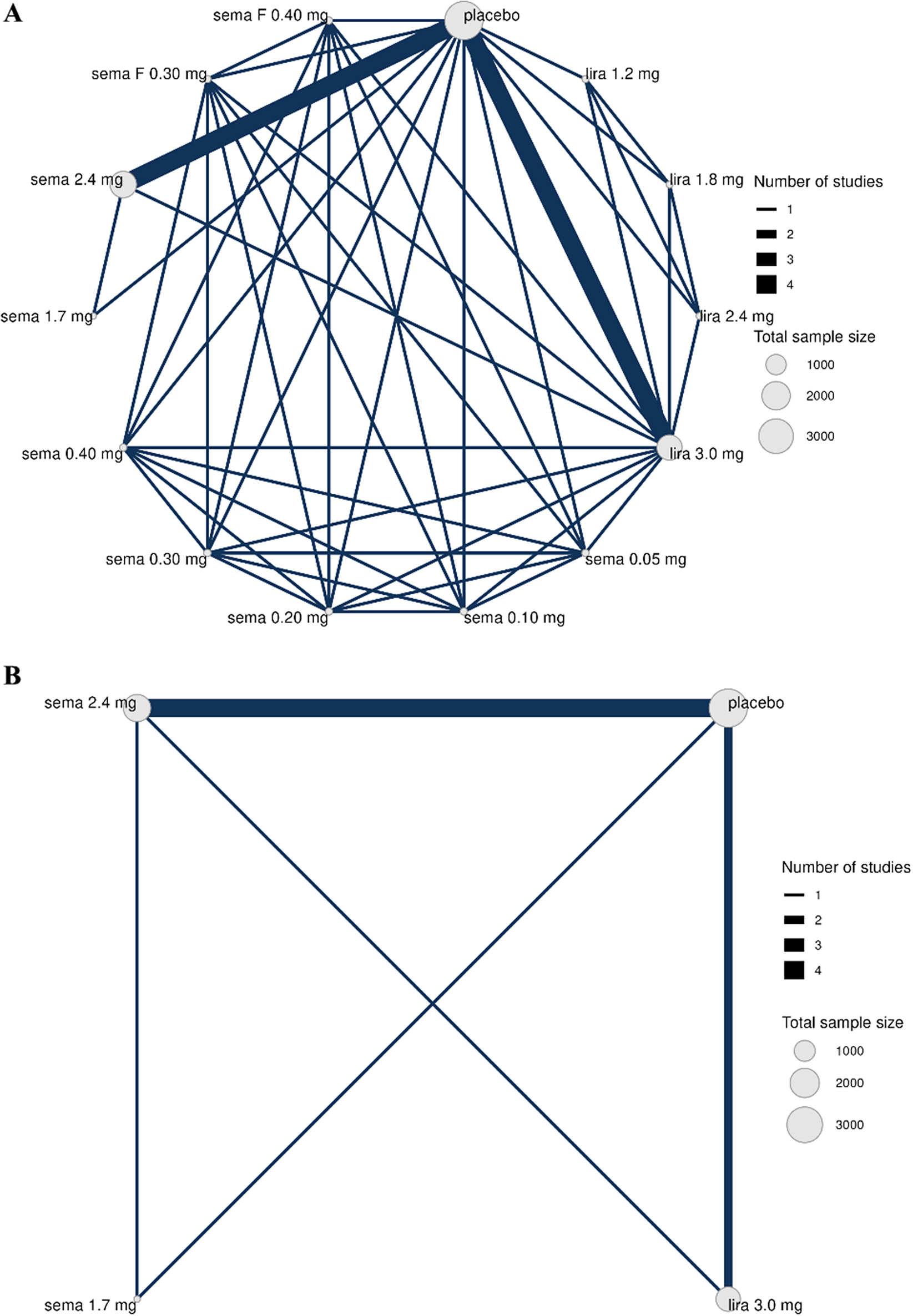
The treatment network is shown in Figure 1, where Figure 1a is the full treatment network and Figure 1a is reduced to phase 3 studies.
Network of treatment comparisons from seven RCTs, where each treatment is represented by a node. Where direct RCT evidence exists for a particular comparison, the nodes are connected by a line, the thickness of which is proportional to the number of comparisons. Network ‘a’ is the full network, including phase 2 and ‘b’ includes only phase 3 data.

Figure 1. Long description
Panel A at the top displays a dense network diagram with eleven nodes labeled placebo, sema F 0.40 mg, sema F 0.30 mg, sema 2.4 mg, sema 1.7 mg, sema 0.40 mg, sema 0.30 mg, sema 0.20 mg, sema 0.10 mg, sema 0.05 mg, lira 1.2 mg, lira 1.8 mg, lira 2.4 mg, and lira 3.0 mg. The largest node is placebo, followed by sema 2.4 mg and lira 3.0 mg, indicating higher total sample sizes. Nodes are connected by lines of varying thickness, with the thickest lines between placebo and sema 2.4 mg, and between placebo and lira 3.0 mg, representing the highest number of direct studies. Thinner lines connect other treatment pairs, forming a highly interconnected web. A legend at the right shows line thickness for 1 to 4 studies and node size for total sample sizes of 1000, 2000, and 3000. Panel B at the bottom shows a simplified network with only four nodes: sema 2.4 mg, placebo, sema 1.7 mg, and lira 3.0 mg. The thickest line connects sema 2.4 mg and placebo. Other lines connect each node to the others, forming a square with diagonals. The same legends for number of studies and sample size appear at the right.
The modelling workflow is defined as follows:
-
1. Time–course models (Table 1) not including a dose–response component are fitted and ranked according to the goodness of fit using the ELPD criterion. First, common-effects models are fitted, followed by the introduction of exchangeable treatment effects, and finally an AR-1 process is introduced for the arm-correlation structure. The dose–response is specified as a set of discrete treatment effects (i.e., a treatment-level MBNMA), making no assumption about the shape of the dose–response, but does assume consistency.
-
2. Based on the best performing time–course model, parametric dose–response models are introduced into the structural parameter of the time–course functions. These models are compared to the treatment-level MBNMA and the UME, using graphical methodsReference Pedder, Dias, Boucher, Bennetts, Mawdsley and Welton 8 and information criteria. For the selected dose–response model in this step, the observed within-arm correlations are introduced and used in the estimation of dose–response parameters.
Two standard NMAs are conducted for comparison purposes. The first uses primary statistical analysis (including imputation of missing data) that was defined in the individual study protocols and evaluated at the per protocol specified end-of-treatment timepoint (spanning from week 56 to week 104). The second uses the aggregated data (as observed) at the per protocol specified end-of-treatment timepoint, which is introduced to align with aggregated time–course data used in the DT-MBNMAs.
2.8 Implementation
Estimation and inference is carried out using Stan (Stan Development Team, version 2.26.1), where the R package brms provides an interface to R (version 2.21.1).Reference Brkner 22 All computations are conducted with R version 4.3.1 (a GitHub repo is available at https://github.com/agorstras/dt-mbnma). Models that included the observed within-arm covariance matrix are implemented directly in Stan because these cannot be fitted with the current version of brms. Choice of prior distributions and convergence diagnostic are presented below and in-detail in the Supplementary Material.
2.9 Convergence monitoring and prior specification
In stochastic simulation and estimation part, two independent chains were run for 1,000 burn-in iterations followed by 1,000 iterations. Gelman’s R statistic was monitored for the model parameters during the simulations, and it appeared that models converged as all parameters had an R < 1.05. In the analysis of the illustrative dataset, two independent chains were run for 2,500 burn-in iterations followed by 2,500 iterations. Gelman’s R statistic was monitored for the model parameters during the simulations, and it appeared that models converged as all parameters had an R < 1.05. If the models did not converge, the number of iterations were tripled.
Vague normal prior distributions with a SD of 100 were given to the nuisance and drug effect parameters (e.g., b or x50, Table 1). For parameters that only take positive values (e.g., time-constants, median effective dose), priors were expressed on a log-scale. The between-study SDs on exchangeable parameters were given half-normal prior distributions with an SD of 5. The prior for correlation matrix for the exchangeable parameters uses the Lewandowski-Kurowicka-Joe prior (LKJ) is used with a degree freedom of 1. In models with a multivariate likelihood, the correlation parameter was given a uniform prior distribution (uniform(–1,1)) to reflect that outcomes at different timepoints within the same study arm are correlated.
3 Results
3.1 Simulation study
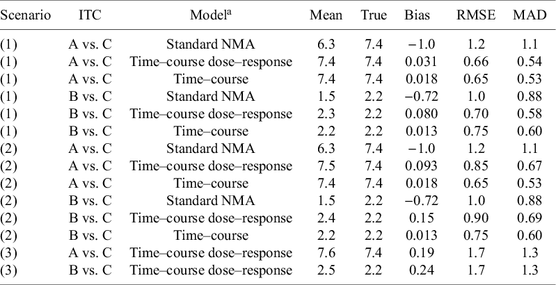
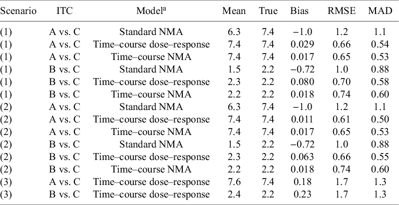
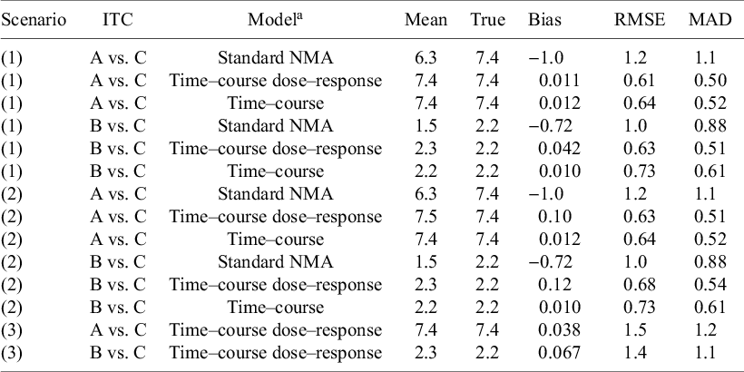
Results of estimation of indirect treatment effects are shown in Tables 2–4. Table 2 depicts the case where within-arm correlations across timepoints are ignored, while Table 3 depicts the case where within-arm correlations across timepoints are approximated with an AR-1 process. Finally, Table 4 displays the case where observed correlations across timepoints are used in the estimation. The T-MBNMA and DT-MBNMA perform similar in terms of both bias and precision of the estimated indirect treatment effects. This is regardless of the correlation structure used in the estimation and across scenarios 1 and 2. Results of estimation of drug effect parameters from simulated data are shown in Figures S3–S5 in the Supplementary Material. Across scenarios 1 and 2, the drug effect parameters are on average estimated without bias because the medians of the individual point estimates (i.e., posterior means) are in line with the true values.
Estimation of indirect treatment comparisons (ITC) under different scenarios: (1) All arms are observed for 52 weeks, (2) Truncate phase 2 for agent C to 28 weeks, and (3) Truncate phase 2 to 28 weeks and exclude phase 3 for agent C

Table 2. Long description
Beginning with scenario 1 at the top, for A versus C, the standard N M A model shows mean 6.3, true 7.4, bias minus 1.0, R M S E 1.2, M A D 1.1. Time–course dose–response model gives mean 7.4, true 7.4, bias 0.031, R M S E 0.66, M A D 0.54. Time–course model yields mean 7.4, true 7.4, bias 0.018, R M S E 0.65, M A D 0.53. For B versus C, standard N M A model has mean 1.5, true 2.2, bias minus 0.72, R M S E 1.0, M A D 0.88. Time–course dose–response model gives mean 2.3, true 2.2, bias 0.080, R M S E 0.70, M A D 0.58. Time–course model yields mean 2.2, true 2.2, bias 0.013, R M S E 0.75, M A D 0.60. Scenario 2, for A versus C, standard N M A model shows mean 6.3, true 7.4, bias minus 1.0, R M S E 1.2, M A D 1.1. Time–course dose–response model gives mean 7.5, true 7.4, bias 0.093, R M S E 0.85, M A D 0.67. Time–course model yields mean 7.4, true 7.4, bias 0.018, R M S E 0.65, M A D 0.53. For B versus C, standard N M A model has mean 1.5, true 2.2, bias minus 0.72, R M S E 1.0, M A D 0.88. Time–course dose–response model gives mean 2.4, true 2.2, bias 0.15, R M S E 0.90, M A D 0.69. Time–course model yields mean 2.2, true 2.2, bias 0.013, R M S E 0.75, M A D 0.60. Scenario 3, for A versus C, time–course dose–response model shows mean 7.6, true 7.4, bias 0.19, R M S E 1.7, M A D 1.3. For B versus C, time–course dose–response model gives mean 2.5, true 2.2, bias 0.24, R M S E 1.7, M A D 1.3. Models are defined in the footnotes. R M S E is root mean square error, M A D is median absolute deviation.
Note: Independence within-arm across timepoints. RMSE, root mean square error; MAD, median absolute deviation.
a
Individual patient data (arm-level) was simulated from an unstructured covariance matrix, generating correlated observations across timepoints. The mean time–course was simulated from an exponential function (
${E}_{max}T\left(1-\exp \left(-\exp (kT)\times time\right)\right)$
 ), where the long-term treatment effect (E
maxT) is dose-dependent and described by an E
max model, having two parameters; maximum response relative to placebo (E
maxD(q)) and the dose at which of half the maximum response can be achieved (ED50(c)) for the 3 agents (q = [A, B, C]). Decay parameter (kT) was dose-dependent and described by a log-linear model, having 1 slope parameter (b(c)). Estimation models (DT-MBNMA and T-MBNMA) assumes a univariate normal likelihood, where within-arm correlations are set to zero.
), where the long-term treatment effect (E
maxT) is dose-dependent and described by an E
max model, having two parameters; maximum response relative to placebo (E
maxD(q)) and the dose at which of half the maximum response can be achieved (ED50(c)) for the 3 agents (q = [A, B, C]). Decay parameter (kT) was dose-dependent and described by a log-linear model, having 1 slope parameter (b(c)). Estimation models (DT-MBNMA and T-MBNMA) assumes a univariate normal likelihood, where within-arm correlations are set to zero.
Estimation of indirect treatment comparisons (ITC) under different scenarios: (1) All arms are observed for 52 weeks, (2) Truncate phase 2 for agent C to 28 weeks, and (3) Truncate phase 2 to 28 weeks and exclude phase 3 for agent C
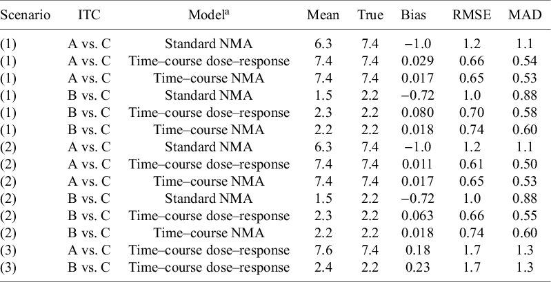
Table 3. Long description
Starting from the top row, the table is organized by scenario number, with each scenario subdivided by treatment comparison (A vs. C or B vs. C) and model type (Standard N M A, Time–course dose–response, Time–course N M A). For scenario 1, A vs. C using Standard N M A has mean 6.3, true 7.4, bias minus 1.0, R M S E 1.2, M A D 1.1. Time–course dose–response and Time–course N M A both have mean 7.4, true 7.4, bias 0.029 and 0.017, R M S E 0.66 and 0.65, M A D 0.54 and 0.53, respectively. For B vs. C, Standard N M A has mean 1.5, true 2.2, bias minus 0.72, R M S E 1.0, M A D 0.88. Time–course dose–response and Time–course N M A have means 2.3 and 2.2, true 2.2, bias 0.080 and 0.018, R M S E 0.70 and 0.74, M A D 0.58 and 0.60. Scenario 2 repeats the same structure: for A vs. C, Standard N M A mean 6.3, true 7.4, bias minus 1.0, R M S E 1.2, M A D 1.1; Time–course dose–response mean 7.4, true 7.4, bias 0.011, R M S E 0.61, M A D 0.50; Time–course N M A mean 7.4, true 7.4, bias 0.017, R M S E 0.65, M A D 0.53. For B vs. C, Standard N M A mean 1.5, true 2.2, bias minus 0.72, R M S E 1.0, M A D 0.88; Time–course dose–response mean 2.3, true 2.2, bias 0.063, R M S E 0.66, M A D 0.55; Time–course N M A mean 2.2, true 2.2, bias 0.018, R M S E 0.74, M A D 0.60. Scenario 3 only includes Time–course dose–response: for A vs. C, mean 7.6, true 7.4, bias 0.18, R M S E 1.7, M A D 1.3; for B vs. C, mean 2.4, true 2.2, bias 0.23, R M S E 1.7, M A D 1.3. The table footnote defines AR-1 as within-arm correlation across timepoints, R M S E as root mean square error, and M A D as median absolute deviation. The simulation note explains that individual patient data were generated using an unstructured covariance matrix, with mean time–course from an exponential function, and dose-dependence modeled by E max and E D 50 parameters for agents A, B, and C. Decay parameter k T is dose-dependent, modeled log-linearly. Estimation models assume multivariate normal likelihood with AR-1 process for within-arm correlations.
Note: AR-1 within-arm correlation across timepoints. RMSE, root mean square error; MAD, median absolute deviation.
a Individual patient data (arm-level) was simulated from an unstructured covariance matrix, generating correlated observations across timepoints. The mean time–course was simulated from an exponential function (
${E}_{max}T\left(1-\exp \left(-\exp (kT)\times time\right)\right)$
 ), where the long-term treatment effect (E
maxT) is dose-dependent and described by an E
max model, having two parameters; maximum response relative to placebo (E
maxD(q)) and the dose at which of half the maximum response can be achieved (ED50(c)) for the 3 agents (q = [A, B, C]). Decay parameter (kT) was dose-dependent and described by a log-linear model, having 1 slope parameter (b(c)). Estimation models (DT-MBNMA and T-MBNMA) assumes multivariate normal likelihood, where within-arm correlations are estimated from aggregated data, using an AR-1 process.
), where the long-term treatment effect (E
maxT) is dose-dependent and described by an E
max model, having two parameters; maximum response relative to placebo (E
maxD(q)) and the dose at which of half the maximum response can be achieved (ED50(c)) for the 3 agents (q = [A, B, C]). Decay parameter (kT) was dose-dependent and described by a log-linear model, having 1 slope parameter (b(c)). Estimation models (DT-MBNMA and T-MBNMA) assumes multivariate normal likelihood, where within-arm correlations are estimated from aggregated data, using an AR-1 process.
Estimation of indirect treatment comparisons (ITC) under different scenarios: (1) All arms are observed for 52 weeks, (2) Truncate phase 2 for agent C to 28 weeks, and (3) Truncate phase 2 to 28 weeks and exclude phase 3 for agent C.
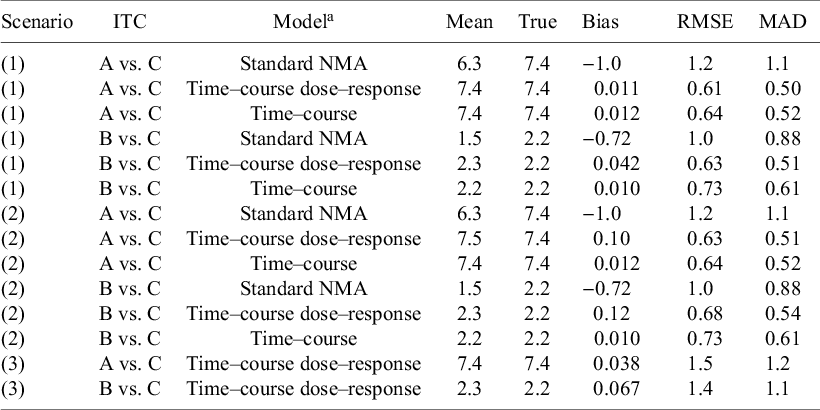
Table 4. Long description
The table contains three scenarios: (1) all arms observed for 52 weeks, (2) phase 2 for agent C truncated to 28 weeks, (3) phase 2 truncated to 28 weeks and phase 3 for agent C excluded. For each scenario, indirect treatment comparisons (A vs. C and B vs. C) are shown for three models: Standard N M A, Time–course dose–response, and Time–course. Columns list Mean, True, Bias, R M S E, and M A D. In scenario 1, for A vs. C, Standard N M A has mean 6.3, true 7.4, bias minus 1.0, R M S E 1.2, M A D 1.1; Time–course dose–response and Time–course both have mean and true 7.4, bias near zero, lower R M S E and M A D. For B vs. C, Standard N M A has mean 1.5, true 2.2, bias minus 0.72, R M S E 1.0, M A D 0.88; Time–course models have means and trues near 2.2, low bias, lower R M S E and M A D. Scenario 2 shows similar patterns, with Time–course models maintaining low bias and error. In scenario 3, only Time–course dose–response models are shown: A vs. C has mean and true 7.4, bias 0.038, R M S E 1.5, M A D 1.2; B vs. C has mean 2.3, true 2.2, bias 0.067, R M S E 1.4, M A D 1.1. Footnotes define R M S E as root mean square error and M A D as median absolute deviation. Models use simulated individual patient data with dose-dependent parameters.
Note: Observed within-arm correlations across timepoints. RMSE, root mean square error; MAD, median absolute deviation.
a Individual patient data (arm-level) was simulated from an unstructured covariance matrix, generating correlated observations across timepoints. The mean time–course was simulated from an exponential function (
${E}_{max}T\left(1-\exp \left(-\exp (kT)\times time\right)\right)$
 ), where the long-term treatment effect (E
maxT) is dose-dependent and described by an E
max model, having two parameters; maximum response relative to placebo (E
maxD(q)) and the dose at which of half the maximum response can be achieved (ED50(c)) for the 3 agents (q = [A, B, C]). Decay parameter (kT) was dose-dependent and described by a log-linear model, having one slope parameter (b(c)). Estimation models (DT-MBNMA and T-MBNMA) assume multivariate normal likelihood, where observed within-arm correlations are used in the estimation.
), where the long-term treatment effect (E
maxT) is dose-dependent and described by an E
max model, having two parameters; maximum response relative to placebo (E
maxD(q)) and the dose at which of half the maximum response can be achieved (ED50(c)) for the 3 agents (q = [A, B, C]). Decay parameter (kT) was dose-dependent and described by a log-linear model, having one slope parameter (b(c)). Estimation models (DT-MBNMA and T-MBNMA) assume multivariate normal likelihood, where observed within-arm correlations are used in the estimation.
The standard NMA model shows lower precision of the estimated indirect treatment effects, but also underestimates the effect size of the indirect treatment effects, when the comparisons are based solely on week 52 data. The systematic underestimation of the effect size, comparing agents A and B to C is expected given the simulation design. In Figure S2A in the Supplementary Material, the true mean time–course profile for higher doses of agent C, the time–course has not reached its nadir (i.e., stabilized), and therefore the full effect size cannot be quantified unless the time–course profile is used and modelled.
In scenario 3, where the phase 2 treatment duration is truncated to 28 weeks and phase 3 data are not available, it appears that there is a minor underestimation of E maxD(c) counteracted by a minor overestimation of drug potency ED50(c) for agent C. These findings are consistent regardless of the correlation structure used to model the underlying IPD. The impact on estimation of indirect treatment effects is minimal as the effect sizes agree with the true values used in the simulations. As expected, the precision on the indirect treatment effects (as measured by RMSE or MAD) is halved, having only phase 2 data available for the ITC. Moreover, it reflects both a smaller study population in phase 2 and a shorter treatment duration.
3.2 Application to the obesity treatment network
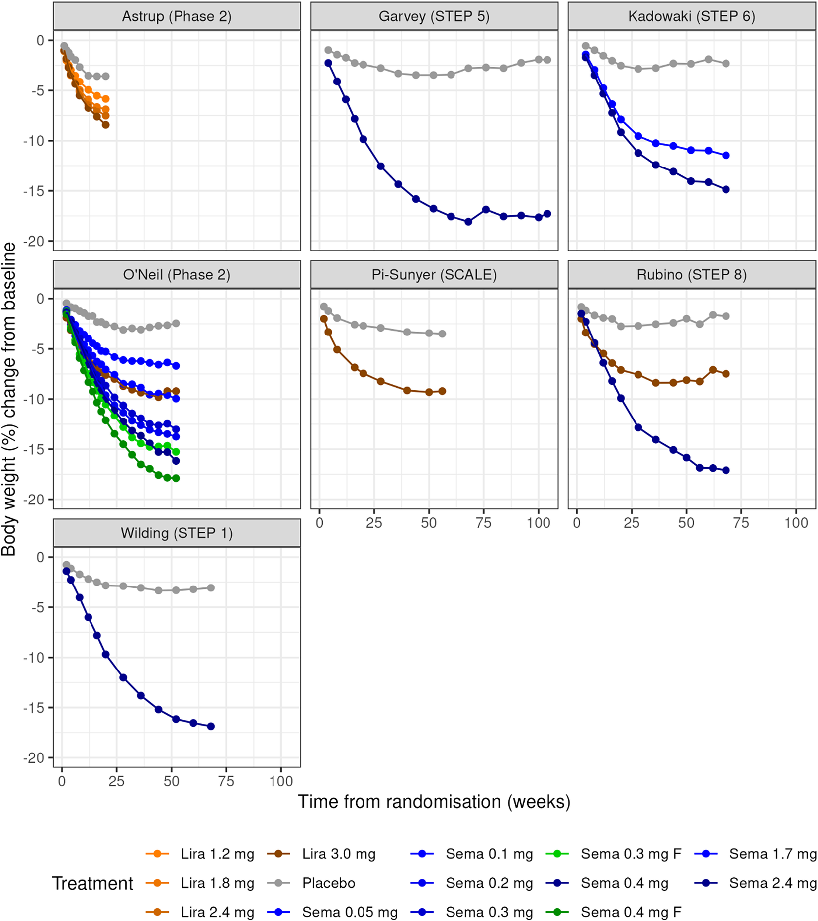
Visual inspection of the data shows that the percent change in BW decreases in a nonlinear time-dependent fashion (Figure 2). In some of the placebo-treated groups, a trend towards baseline levels is observed. This suggests that a simple linear model will not be a good fit for the data, but that E max, exponential, or the Bateman models may be more suitable. Over time, a clear separation of the active treatment arms, showing that the relative effect size of semaglutide and liraglutide increases in a dose-dependent manner (Figure 2).
Plots of body weight change over time for each of the studies in the obesity dataset. Studies are labelled by first author (study name). Panels show the observed mean percentage change from baseline in body weight over time among participants in the full analysis population during the on-treatment observation period. Semaglutide dose levels in O’neil (Phase 2) were standardized to weekly equivalents by multiplying daily doses with 7 to match the once-weekly doses used in phase 3. The treatment labelled ‘F’ represents doses, where semaglutide was dose-escalated in every second to target doses 0.30 mg and 0.40 mg, respectively.
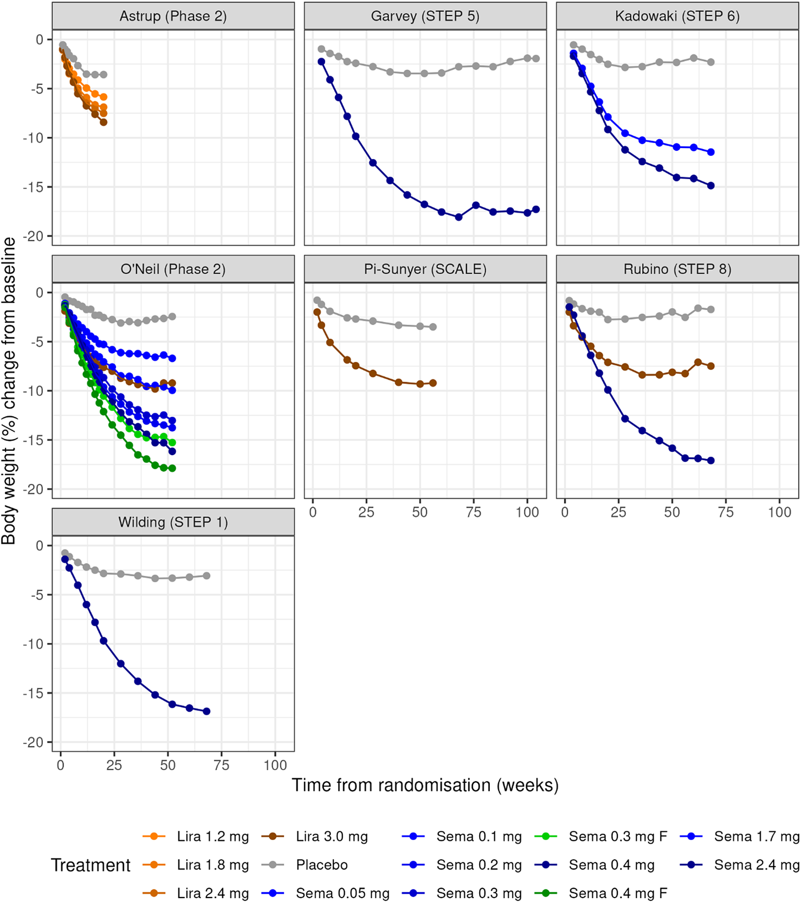
Figure 2. Long description
Starting at the top left, the Astrup (Phase 2) panel shows three orange lines (Lira 1.2 mg, 1.8 mg, 2.4 mg) and one gray line (Placebo), all declining to around minus 7 to minus 10 percent by week 20. Top center, Garvey (STEP 5) displays a blue line (Sema 2.4 mg) dropping to minus 15 percent by week 68, and a gray line (Placebo) remaining near minus 3 percent. Top right, Kadowaki (STEP 6) has three blue lines (Sema 1.7 mg, 2.4 mg, 0.05 mg) and one gray line (Placebo), with the highest dose reaching minus 15 percent. Middle left, O'Neil (Phase 2) shows five lines: three blue (Sema 0.05 mg, 0.1 mg, 0.2 mg), one green (Sema 0.3 mg F), and one green (Sema 0.4 mg F), all declining with higher doses showing greater weight loss, and a gray line (Placebo) near zero. Middle center, Pi-Sunyer (SCALE) has a brown line (Lira 3.0 mg) dropping to minus 8 percent and a gray line (Placebo) near minus 3 percent. Middle right, Rubino (STEP 8) shows a blue line (Sema 2.4 mg) reaching minus 15 percent, a brown line (Lira 3.0 mg) at minus 8 percent, and a gray line (Placebo) near minus 3 percent. Bottom left, Wilding (STEP 1) has a blue line (Sema 2.4 mg) dropping to minus 15 percent and a gray line (Placebo) near minus 3 percent. The x-axis in all panels is time from randomization in weeks, ranging from 0 to 100. The y-axis is body weight percent change from baseline, ranging from 0 to minus 20 percent. The legend at the bottom identifies treatments by color and dose.
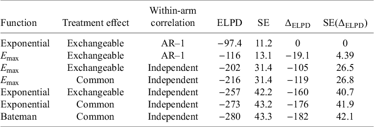
Table 5 gives an overview of the performance of the explored models. The T-MBNMA shows a minor differentiation between E max and exponential models. The Bateman model had convergence problems when exchangeable treatment effects are introduced and therefore not reported. Introducing random effects into the time–course models, facilitating estimation of between-study SD in the structural parameters, shows improvements in the overall fit. Adding within-arm correlations structure in the form an AR-1 process significantly improved the fit to the data with the exponential model performing best. Hence, dose–response models are explored within the exponential time–course model, assuming exchangeable treatment effects and within-arm correlations structure in the form of an AR-1 process. Estimates of the autocorrelation parameter are given in Table 5.
Model fit statistics for time–course models, fitted to the obesity dataset
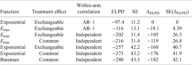
Table 5. Long description
The table contains seven rows and seven columns. Columns from left to right are labeled Function, Treatment effect, Within-arm correlation, E L P D, S E, delta E L P D, and S E of delta E L P D. Row 1: Exponential, Exchangeable, A R dash 1, E L P D negative 97.4, S E 11.2, delta E L P D 0, S E of delta E L P D 0. Row 2: E max, Exchangeable, A R dash 1, E L P D negative 116, S E 13.1, delta E L P D negative 19.1, S E of delta E L P D 4.39. Row 3: E max, Exchangeable, Independent, E L P D negative 202, S E 31.4, delta E L P D negative 105, S E of delta E L P D 26.5. Row 4: E max, Common, Independent, E L P D negative 216, S E 31.4, delta E L P D negative 119, S E of delta E L P D 26.8. Row 5: Exponential, Exchangeable, Independent, E L P D negative 257, S E 42.2, delta E L P D negative 160, S E of delta E L P D 40.7. Row 6: Exponential, Common, Independent, E L P D negative 273, S E 43.2, delta E L P D negative 176, S E of delta E L P D 41.9. Row 7: Bateman, Common, Independent, E L P D negative 280, S E 43.3, delta E L P D negative 182, S E of delta E L P D 42.1. The Exponential function with Exchangeable treatment effect and A R dash 1 correlation has the highest E L P D. E L P D decreases and delta E L P D becomes more negative as models use Independent correlation and Common treatment effect. Table footnote defines E L P D as expected log posterior density estimate and S E as standard error.
Note: ELPD, expected log posterior density estimate; SE, standard error.
Embedding dose–response models for the relative treatment effects on the structural parameters of the exponential time–course model (E maxT and kT) was successful (Table 6). The comparison of DT-MBNMAs to T-MBNMA shows that the dose–response can be captured in a continuous monotonic form with relatively few drug-effect parameters to estimate. The change in the ELPD (ΔELPD) and its corresponding SE indicates that the models are performing equally well.
Model fit statistics for dose–response time–course models, fitted to the obesity dataset

Table 6. Long description
The table contains ten columns: E max T, kT, E L P D, S E, Delta E L P D, S E of Delta E L P D, Between-study S D for E max T, Between-study S D for kT, Correlation between E max T and kT, and Within-arm correlation. The five rows are: Linear/Linear, Log-linear/Log-linear, Treatment level/Treatment level, U M E/U M E, and E max/Log-linear. For all models, E L P D is minus 97 except E max/Log-linear which is minus 98. S E is 11 for all. Delta E L P D ranges from 0 to minus 0.72. S E of Delta E L P D ranges from 0 to 1.5. Between-study S D for E max T ranges from 0.73 [0.038; 2.1] to 1.2 [0.49; 2.1]. Between-study S D for kT ranges from 0.16 [0.0053; 0.56] to 0.18 [0.039; 0.34]. Correlation between E max T and kT ranges from minus 0.15 [minus 0.94; 0.79] to 0.069 [minus 0.94; 0.96]. Within-arm correlation ranges from 0.84 [0.68; 0.95] to 0.86 [0.71; 0.96]. U M E stands for unrelated mean effects model. E L P D is expected log posterior density estimate. S E is standard error.
Note: ELPD, expected log posterior density estimate; SE, standard error; UME, unrelated mean effects model.
a The exponential function
${E}_{max}T\left(1-\exp \left(-\exp (kT)\times time\right)\right)$
 is specified for the time–course relationship.
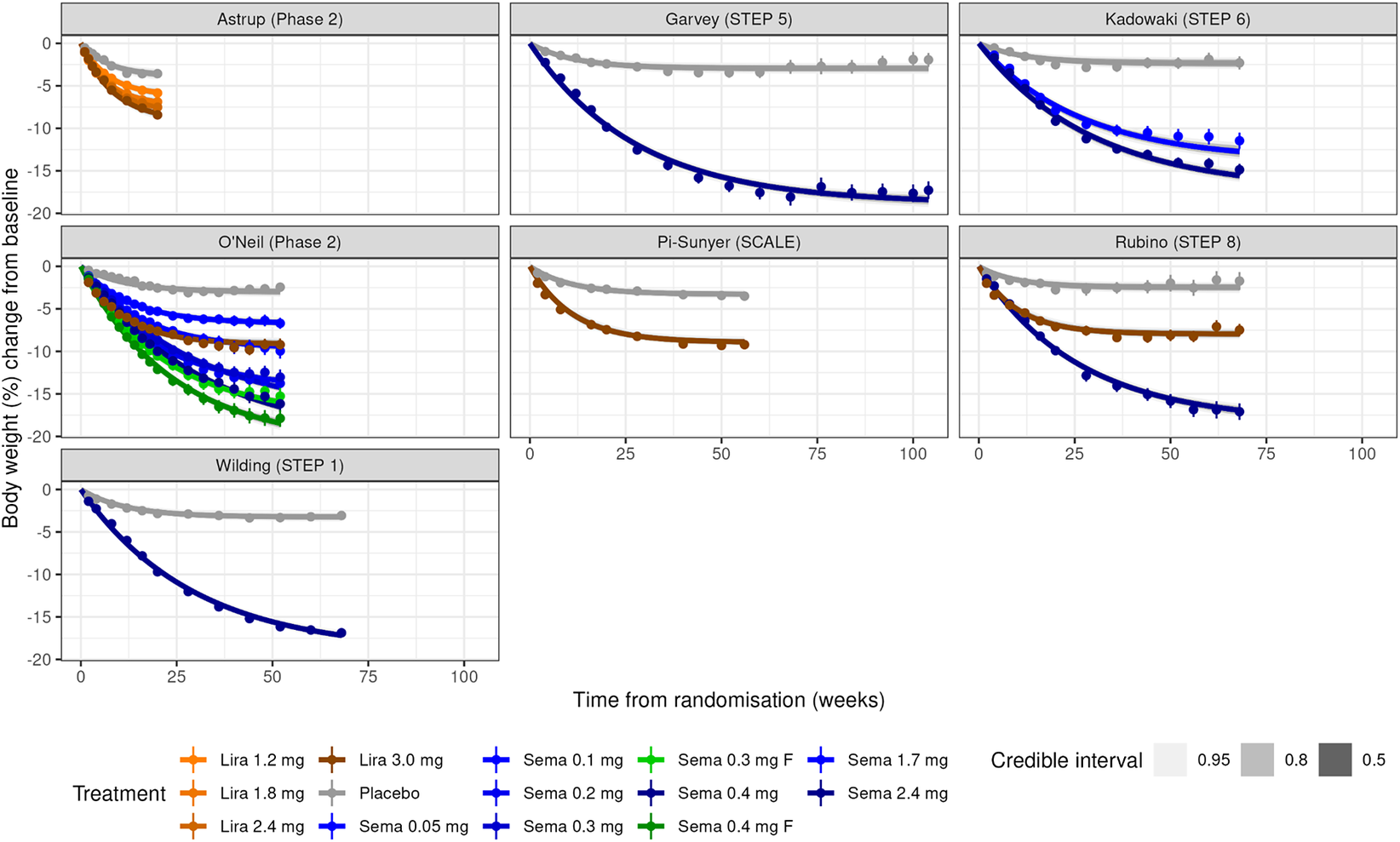
The DT-MBNMAs show a minor differentiation between log-linear and E max model in terms of the between-study SDs for E maxT and Kt, and that the SDs were in line with the T-MBNMA and UME models. This indicates that there are no major violations of assumptions around the dose–response relationship and the consistency assumption. Fitting a linear dose–response model shows that the between-study SD on the time–course parameter (E maxT) increases substantially, indicating that heterogeneity between studies increases as consequence of a poor performing dose–response function. Embedding an E max function on both time–course parameters (E maxT and kT) to model the dose–response had convergence problems and is therefore not reported. In Figure 3, the VPCs (Visual Predictive Check) are displayed, and in Figure S6 in the Supplementary Material, deviance–deviance plot is shown for relevant dose–response models compared to the UME. Additionally, the individual studies are provided in Figures S7–S12 in the Supplementary Material, providing more insight into model performance. This suggests that DT-MBNMA adequately described the summary-level data for all study arms.
Plots of body weight change over time for each of the studies in the obesity dataset. Studies are labelled by first author (study name). Panels show the observed mean percentage change from baseline in body weight over time among participants in the full analysis population during the on-treatment observation period. Lines are model posterior means and credible intervals.

Figure 3. Long description
There are seven panels arranged in three rows and three columns, with the bottom right cell empty. Each panel is labeled at the top with the study name and phase: Astrup Phase 2, Garvey STEP 5, Kadowaki STEP 6, O'Neil Phase 2, Pi-Sunyer SCALE, Rubino STEP 8, and Wilding STEP 1. The x-axis of each panel is labeled Time from randomisation in weeks, ranging from 0 to 100. The y-axis is labeled Body weight percent change from baseline, ranging from 0 to negative 20. Each panel contains multiple lines representing different treatments: orange for Lira 1.2 mg, Lira 1.8 mg, Lira 2.4 mg, Lira 3.0 mg; blue for Sema 0.05 mg, Sema 0.1 mg, Sema 0.2 mg, Sema 0.3 mg F, Sema 0.4 mg, Sema 0.4 mg F, Sema 1.7 mg, Sema 2.4 mg; and gray for Placebo. Each line shows the observed mean percentage change in body weight over time, with model posterior means and shaded credible intervals in three shades of gray for 0.95, 0.8, and 0.5. In all panels, placebo groups (gray) show minimal weight change, while active treatments (especially higher dose Sema in blue) show greater and sustained weight loss over time. The legend at the bottom identifies each treatment and credible interval shading.
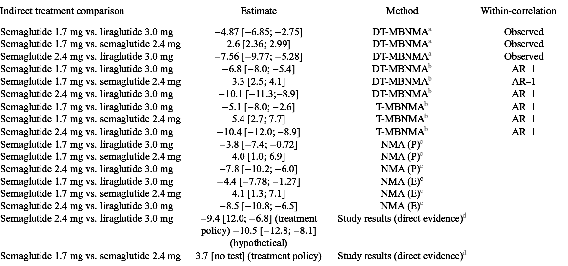
ITC between different liraglutide and semaglutide doses that are approved for the treatment of obesity 12 , 13 are presented in Table 7. With the MBNMA approach, we can rank agents at any given dose on both structural parameters in the exponential time–course function, but we are interested in treatment nadir (i.e., long-term weight loss), and hence dose-dependent effects on the E maxT parameter are used for the ITC. The relative effect of semaglutide 2.4 mg vs. liraglutide 3 mg is in line with study levels results from Rubino (STEP 8), showing that semaglutide 2.4 mg provides a superior weight reduction compared to liraglutide 3 mg.Reference Rubino, Greenway and Khalid 21 The relative effect of semaglutide 1.7 mg vs. semaglutide 2.4 mg is in line with study levels results from Kadowaki (STEP 6).Reference Kadowaki, Isendahl and Khalid 20 There is no direct evidence for comparison of semaglutide 1.7 mg vs. liraglutide 3 mg. Both methods (T-MBNMA and NMA) indicate that semaglutide 1.7 mg provides a superior weight reduction compared to liraglutide 3 mg, but the relative treatment effect appears larger with DT-MBNMA method. Here the difference between the two methods is clearer in the sense that the DT-MBNMA uses information from the full treatment network (i.e., phase 2 and phase 3, Figure 1a) to estimate the dose–response relationship for both agents, whereas NMA is informed only by phase 3 data, where the treatment effect of semaglutide 1.7 mg is only observed and reported in the Kadowaki (STEP 6) study. Therefore, the ITC of semaglutide 1.7 mg vs. liraglutide 3.0 mg can be done with greater precision because the treatment comparisons are computed from the agent specific dose–response curves, being summarized in only two drug effect parameters.
Indirect treatment comparison (ITC) between different liraglutide and semaglutide doses that are approved for the treatment of obesity
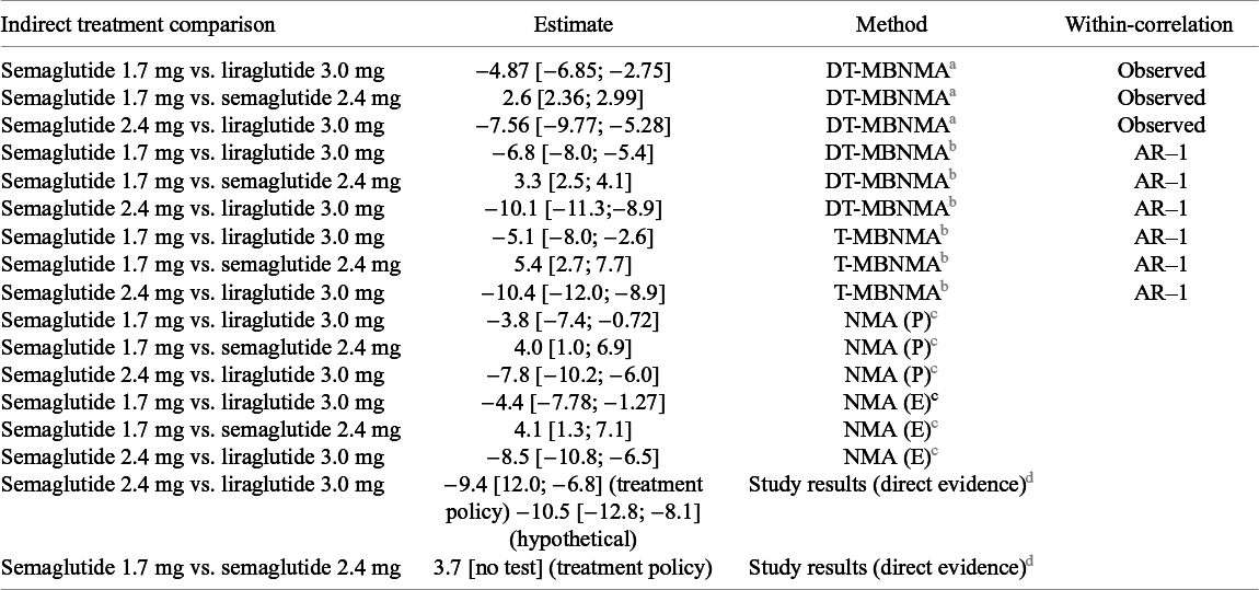
Table 7. Long description
The table contains 17 rows and 4 columns. Columns from left to right are: Indirect treatment comparison, Estimate, Method, and Within-correlation. The first three rows use the DT-M B N M A method with observed correlation: Semaglutide 1.7 mg vs. liraglutide 3.0 mg, estimate negative 4.87 [negative 6.85 to negative 2.75]; Semaglutide 1.7 mg vs. semaglutide 2.4 mg, estimate 2.6 [2.36 to 2.99]; Semaglutide 2.4 mg vs. liraglutide 3.0 mg, estimate negative 7.56 [negative 9.77 to negative 5.28]. The next three rows use DT-M B N M A with AR-1 correlation: Semaglutide 1.7 mg vs. liraglutide 3.0 mg, estimate negative 6.8 [negative 8.0 to negative 5.4]; Semaglutide 1.7 mg vs. semaglutide 2.4 mg, estimate 3.3 [2.5 to 4.1]; Semaglutide 2.4 mg vs. liraglutide 3.0 mg, estimate negative 10.1 [negative 11.3 to negative 8.9]. The next three rows use T-M B N M A with AR-1: Semaglutide 1.7 mg vs. liraglutide 3.0 mg, estimate negative 5.1 [negative 8.0 to negative 2.6]; Semaglutide 1.7 mg vs. semaglutide 2.4 mg, estimate 5.4 [2.7 to 7.7]; Semaglutide 2.4 mg vs. liraglutide 3.0 mg, estimate negative 10.4 [negative 12.0 to negative 8.9]. The next three rows use N M A (P): Semaglutide 1.7 mg vs. liraglutide 3.0 mg, estimate negative 3.8 [negative 7.4 to negative 0.72]; Semaglutide 1.7 mg vs. semaglutide 2.4 mg, estimate 4.0 [1.0 to 6.9]; Semaglutide 2.4 mg vs. liraglutide 3.0 mg, estimate negative 7.8 [negative 10.2 to negative 6.0]. The next three rows use N M A (E): Semaglutide 1.7 mg vs. liraglutide 3.0 mg, estimate negative 4.4 [negative 7.78 to negative 1.27]; Semaglutide 1.7 mg vs. semaglutide 2.4 mg, estimate 4.1 [1.3 to 7.1]; Semaglutide 2.4 mg vs. liraglutide 3.0 mg, estimate negative 8.5 [negative 10.8 to negative 6.5]. The final two rows are study results (direct evidence): Semaglutide 2.4 mg vs. liraglutide 3.0 mg, estimate negative 9.4 [12.0 to negative 6.8] for treatment policy and negative 10.5 [negative 12.8 to negative 8.1] for hypothetical; Semaglutide 1.7 mg vs. semaglutide 2.4 mg, estimate 3.7 [no test] for treatment policy. Methods are defined in the footnotes: D T-M B N M A and T-M B N M A use an exponential function for time-course; N M A (P) and N M A (E) use trial-level estimates; AR-1 indicates an autoregressive correlation model. All estimates are presented as posterior mean with 95 percent credible intervals.
a The exponential function
${E}_{max}T\left(1-\exp \left(-\exp (kT)\times time\right)\right)$
 is specified for the time–course relationship. Treatment contrasts are derived from the semaglutide- and liraglutide-specific log-linear dose–response functions. The within-arm correlation was the observed within treatment arm .
b
The exponential function
${E}_{max}T\left(1-\exp \left(-\exp (kT)\times time\right)\right)$
 is specified for the time–course relationship. Treatment contrasts are derived from the semaglutide- and liraglutide-specific E
max dose–response functions or agent-by-dose combinations. The within-arm correlation was the observed approximated with an AR-1 process.
is specified for the time–course relationship. Treatment contrasts are derived from the semaglutide- and liraglutide-specific E
max dose–response functions or agent-by-dose combinations. The within-arm correlation was the observed approximated with an AR-1 process.
c The Standard NMA analysis used two datasets: (P) trial level estimates from the primary estimand specified per protocol and (E) trial level estimates from the end-of-treatment visit as observed, to align with the data used in MBNMA. MBNMA and NMA estimates are presented as posterior mean with 95% credible intervals in brackets.
d Trial level results comparing semaglutide 1.7 mg vs. semaglutide 2.4 mg in STEP 6 and semaglutide 1.7 mg vs. semaglutide 2.4 mg in STEP 8.
Finally, because IPD were available for these illustrative trials, we computed the observed within-arm correlation matrices to assess sensitivity of the results to the correlation specification. This is used in the estimation of drug effect parameters and thus of indirect treatment effects. The use of observed within-arm correlation structure had limited effects on the relative treatment effects under the DT-MBNMA approach. This is in line with results from the simulation study.
4 Discussion
4.1 Joint estimation of dose–response and time–course relationship
The purpose of the simulation study was to demonstrate that the drug effect parameters can be estimated jointly with time–course parameters that may be dose-dependent, while respecting randomization. Simulations show that drug effect parameters can be estimated reliably and with low bias. The precision of the drug effect parameters and therefore indirect treatment effects is affected by the quantity and location of observations at a given set of timepoints. These findings are consistent with the results of an extensive simulation study,Reference Pedder, Boucher, Dias, Bennetts and Welton 23 investigating aspects of the aggregate data for parameter identifiability. We refer to Pedder et al.Reference Pedder, Boucher, Dias, Bennetts and Welton 23 for a discussion on how T-MBNMA parameters were affected by the quantity and location of observed timepoints across studies. In addition, we have also shown how the observed within-arm correlations can be used in the aggregated data analysis although the information is seldom available in publications.
Convergence failure was not observed in any of the simulated datasets, which can be attributed to the simulation setup. It must be noted that three or more doses are required to be tested in the RCTs to estimate a dose–response relationship (e.g., Figure S2B in the Supplementary Material) and preferably the included RCTs should cover a broad dose-range. For instance, optimal experimental design theory has shown that to estimate parameters ED50 and E max with the highest precision, then a dose should be located at the point of median effective dose and a dose should be located at the point, where the response is plateauing. Therefore, it is expected that in the design of individual dose-finding studies, careful consideration is given to the number and location of doses in the grid, enabling dose–response functions to be fitted for the characterization of the dose–response relationship for a given agent. Proof-of-concept studies typically test a single high dose against placebo and can be included directly in the analysis to provide evidence on maximal efficacy, though they contribute no information for dose–response parameter estimation. Alternatively, such studies may inform hierarchical priors or sensitivity analyses.
Future research should systematically evaluate the framework’s performance under dose–response misspecification. While we demonstrate unbiased recovery under correct specification and provide tools to detect misspecification (ELPD, between-study heterogeneity diagnostics), simulations systematically quantifying bias when incorrect functional forms are fitted would complement this work.
The framework accommodates agent-specific parameters with the possibility of combining these into shared parameters or class-effect parameters. Hence, information on dose–response characteristics can be inferred from other agents by assuming varying degrees of similarity and thus improving parameter identifiability. In a reimbursement context, ITCs frequently need to make auxiliary assumptions to have a connected network. For example, windows for analysis timepoints may need to be defined; otherwise, the treatment network will be disconnected. Such windows may differ from the decision problem and/or introduce bias. A parametric time–course component allows the inclusion of all timepoints, and predictions can be made at timepoints relevant for the decision.
We have shown how the NMA framework can be extended using ideas from the MBMA literature to incorporate both dose–response and time–course models in a coherent manner. The framework is used to analyse data from seven RCTs in the treatment of obesity with GLP-1 RAs, covering a wide dose span and end-of-treatment timepoints varying from 20 weeks to 104 weeks. In a standard NMA, phase 2 would have been excluded due to the short treatment duration even though a licensed dose (i.e., liraglutide 3.0 mg) was included in the Astrup 2009 trial.Reference Astrup, Rossner and Van Gaal 6 As illustrated here, all available evidence is integrated with the MBNMA method at the expense of additional assumptions on the parametric forms for the time–course relationship. We have used a ‘staged’ approach for model selection as advocated by Pedder et al.,Reference Pedder, Dias, Bennetts, Boucher and Welton 3 , Reference Pedder, Boucher, Dias, Bennetts and Welton 23 and the selected DT-MBNMA is compared to the T-MBNMAs that do not make any assumptions of the shape of the dose–response. As an alternative to this approach, Bayesian model averaging (BMA) may be an attractive method. BMA is a statistical method used to address model uncertainty in the context of model selection. Rather than selecting a single ‘best’ model, BMA considers a set of candidate models and accounts for uncertainty by averaging over the predictions of multiple models, weighted by their posterior probabilities. The methodology has recently been employed in dose–response modellingReference Gould 24 and meta-analysis applicationsReference Gronau, Heck, Berkhout, Haaf and Wagenmakers 25 and could be explored for MBNMA.
Joint modelling of dose–response and time–course relationships requires sufficient data across both the dose and time dimensions. Our obesity case study demonstrates a setting where the framework is applicable. However, therapeutic areas with sparse phase 2 evidence, limited dose ranges in published trials, or few intermediate timepoints may lack the data needed for reliable estimation. In such cases, simpler approaches (standard NMA with timepoint windows or separate dose–response and time–course models) may be preferable. Importantly, the framework can also be used to tackle heterogeneous treatment durations and dose selections within phase 3 evidence, which would otherwise require arbitrary timepoint windows or disconnect the network.
4.2 The role of model-based network meta-analysis in drug development
The approach described in this paper can be used in model-informed drug development as a platform for evaluation of indirect comparative efficacy and safety information. For example, to evaluate a proposed phase 3 trial comparing dose X to comparator Y at 52 weeks, we simulate outcomes by drawing from the DT-MBNMA posterior predictive distribution of treatment effects at the planned dose and timepoint. The Bayesian formulation captures both parameter uncertainty (from the dose–response and time–course models) and between-trial heterogeneity, enabling estimation of power or probability of success for the planned design. Such simulations can inform dose selection and sample size requirements by quantifying uncertainty in expected treatment effects for designs not yet tested. While we have focused on estimating indirect treatment effects, the framework also enables prediction of absolute time–course profiles for specific doses and timepoints.
5 Conclusion
We have devised a statistically robust framework that combines dose–response MBNMA and T-MBNMA. The resulting DT-MBNMA framework utilizes parametric models to formalize Bayesian evidence synthesis across trials with between-trial differences in assessment timepoints and dose levels. In addition to being useful for informing decision-making in clinical development, the DT-MBNMA framework is a valuable addition to the HTA toolbox, enabling stronger integration of evidence.
Competing interest statement
The authors declare that they are shareholders in Novo Nordisk A/S.
Author contributions
Conceptualization: A.S., M.B., A.G.-R.; Data curation: A.S., M.B., A.G.-R.; Formal analysis: A.S., M.B., A.G.-R.; Methodology: A.S., M.B., A.G.-R.; Software: A.S.; Writing—original draft: A.S.; Writing—review and editing: A.S., M.B., A.G.-R.
Data availability statement
The program code file and simulated dataset can be found at https://zenodo.org/records/19850316.
Funding statement
The project was internally supported by Novo Nordisk A/S.




 Open access

