


21.1 Introduction
Rhythm in speech is the temporal structure created by patterns of variation in duration, fundamental frequency (f0), and intensity. These patterns can result from articulatory processes (Tilsen, Reference Tilsen2019), characteristics of the spoken language (Cutler et al., Reference Cutler, Dahan and Van Donselaar1997), and pressures arising from comprehension processes (see Chapters 18 and 19). The rhythmic patterns in naturally produced speech vary both within and between speakers.
In instances where we wish to control or manipulate speech prosody, this natural variation presents a challenge. For example, if contrasting the effect of different intonational contours on speech perception, it would be necessary to ensure that non-temporal parameters (f0, intensity, phonation type) are not correlated with temporal patterns that could offer an alternative interpretation of effects. Conversely, if contrasting different temporal patterns, it would be necessary to ensure that the independent variable is not confounded by non-temporal parameters.
Faced with this type of challenge, there are four options: to record speech produced by a trained phonetician, to synthesise speech, to alter the timing of a speech recording (retiming), or some combination of these (e.g., the retiming and resynthesis of speech produced by a trained phonetician in Smith and Rathcke, Reference Smith and Rathcke2017). Speech produced by a phonetician or by speech synthesis are both valuable tools for research. However, even trained phoneticians may not be able to control timing very precisely, whereas controlling timing in synthetic speech requires a priori decisions to be made in the parametrisation of the tool. In contrast, retiming speech can produce multiple signals with different temporal characteristics from a single source.
Although it would be preferable to avoid signal degradation or disruption of local prosody, there are ways of mitigating the impact. One approach is to counterbalance these effects across experimental conditions. For example, when producing isochronous stimulus items, Aubanel et al. (Reference Aubanel, Davis and Kim2016) created a matched anisochronous condition with the same amount of absolute temporal distortion. While this allows for comparisons between different retimings, it does not allow for naturalistic stimulus design. A further risk is that the experimental manipulation is more apparent to the participant.
Where it is a priority that stimuli sound natural, it is important to consider subtle differences in how a retiming might affect an utterance. Two important factors to this are the amount of disruption to the signal and the location of the disruption. The least disruptive retiming would be no retiming at all, with the most disruptive retimings approaching the hypothetical physical limits of the transformation where parts of the signal are sped or slowed by infinite factors. Therefore, a possible approach is to perform the minimally disruptive retiming that achieves the desired temporal structure. However, extreme disruptions may have subtle effects in certain positions. For example, a part of a signal sped by an infinite factor would be equivalent to the removal of that part of the signal. In most cases this would be an unacceptable disruption to the signal. However, there would be special cases with ecologically valid interpretations, such as retiming a recording of the word LIBRARY produced as /laɪbrəri/ in a manner that results in the elision of the medial syllable to produce /laɪbri/, amounting to complete deletion of one or more segments, as observed for many phenomena cross-linguistically (e.g., Johnson, Reference Johnson, Yoneyama and Maekawa2004; Dilley and Pitt, Reference Dilley and Pitt2010; Bürki et al., Reference Bürki, Ernestus, Gendrot, Fougeron and Frauenfelder2011; Turnbull, Reference Turnbull2018). Similarly, infinite slowing of a section of the signal would be an extreme disruption, but at a word or syntactic boundary, it would be equivalent to a speaker taking a pause (Zellner, Reference Zellner and Keller1994; Kentner et al., Reference Kentner, Franz, Knoop and Menninghaus2023). These retimings may be subtle in the sense that they would not necessarily sound unusual, but if not applied with careful consideration of the prosodic context, they could result in unacceptable disruptions to the signal.
The aim of this chapter is to provide an overview of the possibilities available to researchers producing retimed stimuli. Three methods of producing retimed stimuli are presented and their utility is demonstrated by creating utterances to have an isochronous rhythm. It is expected that all three methods will enhance the periodicity of the utterances to match the frequency implied by the isochronous intervals. Following this, we present an example of how the last of these three methods may be generalised to produce a wider variety of stimulus types.
21.2 Isochronous Speech
21.2.1 Materials
A corpus composed of a male speaker of Scottish English producing simple mathematical sums was recorded and segmented into words for the purpose of demonstrating the three retiming methods. The corpus was composed of all 66 possible correct sums containing only the numbers from ONE to TEN, and the operators indicated by the words PLUS, MINUS, and IS, for example, FOUR PLUS FIVE IS NINE or THREE MINUS TWO IS ONE. All sums containing SEVEN were excluded, leaving MINUS (produced as /ˈmaɪnəs/) as the only polysyllabic word. Sums were spoken with a quasi-isochronous rhythm at an approximate rate of one word per second with short silences between words.
21.2.2 Retiming Methods
Three approaches to retiming speech are considered here. In each case the interval between perceptual centres (p-centres; Morton et al., Reference Morton, Marcus and Frankish1976; Chapter 11) is held constant at one second. Here, p-centres are defined as the maximum rate of change of the amplitude envelope for a syllable; however, these approaches could be applied to alternative definitions. The first method achieves isochronous retiming by increasing the rate of the entire utterance and extending or inserting silences. The second method alters the rate of the signal between p-centres, and the third method continuously varies the rate of the speech.
In order to compare these methods, we applied them to create stimuli with the shared specification that the p-centres of each word should be equally spaced to achieve an isochronous utterance. For this reason, the term anchor point is used here somewhat interchangeably with the term p-centre. However, these methods are not limited to producing isochronous stimuli. Any feature that can be annotated as a fixed point could be used if there is a motivation to control the timing of the associated event.
Isochrony has advantages for the purposes of evaluation. The effectiveness of the retiming technique can be measured by the extent to which the signal is made more isochronous. Isochrony is defined in the time domain as a signal with equal time intervals between events and can be measured using autocorrelation.Footnote 1 Furthermore, isochrony would also be expected to be observable in the frequency domain as the rate of intervals per unit time. This can be measured using discrete Fourier transformation (DFT). Typically, the DFT representation will show a high level of spectral power at the frequency corresponding to the interval between events. There are, however, potential theoretical implications for the choice of measure. A DFT decomposes a signal into sinusoidal waves whether or not the signal is composed of sinusoidal waves. As a result, it may not be best suited to detect recurrences of irregular waveforms (Zhou et al., Reference Zhou, Melloni, Poeppel and Ding2016). For example, the amplitude envelope of an utterance with a regular one-second interval between syllables would typically have high spectral power at a frequency of 1 Hz. However, an irregular signal could have a high concentration of spectral power at 1 Hz because of a strong 1 Hz component to the signal such as a single cycle of a 1 Hz sinusoidal wave repeating at irregular intervals. In contrast, evaluating isochrony in the time domain using autocorrelation will capture recurrences even if no sinusoidal pattern is apparent in the amplitude envelope.
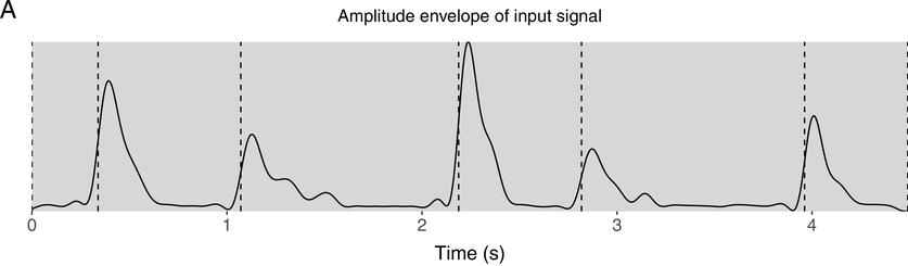
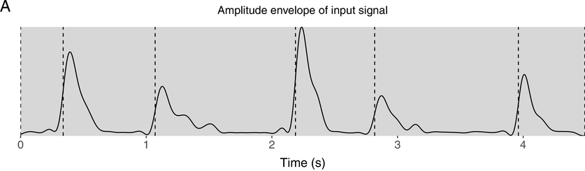
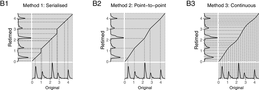
To provide a representation of the rhythmic structure of the input signals, the amplitude envelope was extracted using the extract_env function from the retimer package (Beith, Reference Beith2022). This function is an implementation of the vocalic envelope extraction method proposed by Tilsen and Johnson (Reference Tilsen and Johnson2008), with the additional option to control the low-pass filter and output sampling frequency. These modifications make it possible to extract a smoothed envelope by setting the sampling frequency higher than the low-pass filter frequency. Onsets were then detected by finding peaks in the rate of change in amplitude. An amplitude envelope of an example utterance is shown in the upper panel of Figure 21.1, annotated with the p-centres that are used as anchor points.
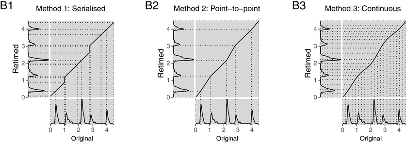
Retiming warp paths.
Upper panel (A) shows the amplitude envelope of the input signal annotated with p-centre estimates.
Lower panel (B) shows the mapping of each of the three retimings (left axes) to the input signal (bottom axes).
All retimings were performed in R with the wsola function from the retimer package. This function is a translation of the wave-similarity overlap-and-add algorithm (WSOLA) implemented in the TSM (time-scale modification) toolbox (Driedger and Müller, Reference Driedger and Müller2014) for Matlab. A translation for Python users is also available in the PyTSMod library (PyTSMod, 2022). Like OLA, WSOLA involves overlapping windowed slices of the signal to compress or extend the duration of a part of the signal. The advantage of WSOLA is that it allows the positioning of the overlaps to be adjusted to minimise phase discontinuity. The techniques discussed here could also be applied to any retiming algorithm implemented in either the TSM toolbox or PyTSMod. Additionally, an OLA transformation can also be produced by using the WSOLA with the tolerance parameter set to 0 (Driedger and Müller, Reference Driedger and Müller2014). Many speech researchers will also be familiar with time-domain pitch-synchronous overlap-and-add (TD-PSOLA; Valbret et al., Reference Valbret, Moulines and Tubach1992) due to its implementation in Praat (Boersma and Weenink, Reference Boersma and Weenink2023). This method performs a source-filter decomposition, which makes it additionally useful for pitch transformations, but still shares the limitations of OLA in terms of phase discontinuities.
21.2.2.1 Method 1: Serialisation
Most simply, what is referred to here as serialisation is an utterance that is created by presenting individual words in a sequence. This is the same stimulus presentation method that led to the observation that an utterance created with regularly spaced word onsets does not result in a perceptually regular utterance (Morton et al., Reference Morton, Marcus and Frankish1976). It is also an auditory analogue to the common rapid serial visual presentation paradigm (RSVP; Potter, Reference Potter1984).
Despite the intuitive appeal of this method, the actual process of producing stimulus items can be challenging. Altering the temporal position of a word in a continuous utterance without silences at word boundaries will result in an overlap with one of the neighbouring words. Therefore, to prevent overlaps, either the rate of words must be increased to shorten their durations or the length of the utterance must be increased to provide additional space.
The implementation presented here is constrained by the previously mentioned requirement that the p-centres of each word are equally spaced by a fixed interval of one second. The function used here is provided in the retimer package (Beith, Reference Beith2022) as get_serial_anchors(). It takes two sets of anchor points in seconds – corresponding to the original p-centres and desired p-centres – as arguments, along with the onsets and offsets of the words. This assumes that there is silence between words in the original utterance or that the researcher has inserted silences prior to the transformation. The function calculates the minimum reduction in speech rate that will prevent overlaps and returns a set of anchor points corresponding to word onsets and offsets that will result in the desired p-centre alignment. If a sample rate is provided, these anchors are transformed to index time in samples rather than seconds. A retiming factor can also be provided if – as is the case here – all items are to be retimed by a common factor. The resulting anchor points, along with the input signal and sample rate, can then be passed to the wsola function to return the retimed signal.
An alternative approach would be to use the anchor points returned by get_serial_anchors() or an equivalent calculation to individually present words or concatenate signals with silence. Presenting individual words may be more appropriate when generating stimuli in real time during an experiment. However, concatenation may also require the insertion of spectrally matched noise rather than silences.
21.2.2.2 Method 2: Point to Point
A logical progression from method 1 would be to relax the constraint that the rate increase applied to each word is uniform across words. However, the benefits of this approach would be limited as the necessary rate increase to prevent overlaps would be constrained by the position of neighbouring words. Therefore, it would still be necessary to insert silence in most cases. A solution to this is to annotate the utterance from p-centre to p-centre and apply the retiming to these intervals.
One of the advantages of this method over method 1 is that there is no need to rely on heuristics to calculate anchors without overlaps. The researcher is required only to provide a list of anchors referring to the p-centres in the input signal and a list of anchors referring to the desired timing of the p-centres in the output signal.
As this method does not insert any silence, or change overall utterance duration, there is no change to the average rate of the utterance. Instead, sections that are sped are compensated for by sections that are slowed. Additionally, the durations of pauses between words are preserved relative to the surrounding context. The cost of this is that tempo can change within a word and phone as p-centres are not typically located at word or even phone boundaries. This discontinuity in the speech rate will be most pronounced when the speech rate in the source recording alternates between fast and slow, as this would result in one part of the word being sped and another part slowed.
21.2.2.3 Method 3: Continuous
In the first method there was a discontinuity in time as silences interrupted the speech. In the second method there was a discontinuity in rate as fast intervals followed slow and slow followed fast. Method 3 smooths the transitions at rate changes by continuously altering the speech rate.
A convenient way of achieving this is to interpolate a spline passing through the same anchor points as would be used in the prior method. A spline provides a smooth, continuous function between anchor points so that abrupt discontinuities are avoided. In some cases, fitting a spline could result in a set of anchors that would imply that parts of the signal were to be reversed. This can be avoided by using the spline algorithm proposed by Hyman (Reference Hyman1983) that fits a cubic spline to a series of points while preserving the monotonicity of the input. This algorithm is available as the spline function in R and through the SciPy (Virtanen et al., Reference Virtanen, Gommers and Oliphant2020) library for Python.
21.2.3 Analysis
Each of these three retiming methods will result in the desired p-centre onset time. However, they do so with different degrees of temporal distortion and with differences in the distribution of these distortions over the duration of the utterance.
Retimings can be visualised by plotting the warp path of the original and retimed speech. The warp path is given by the intersection of matched points projected from adjacent axes, as shown in the lower panel of Figure 21.1.
The first method results in a warp path made up of two types of lines: the diagonal segments that are all projected at a common angle corresponding to the retiming factor, and the vertical segments corresponding to insertions of silence. This is indicative of a discontinuity in the speech itself. In contrast, the warp path resulting from method 2 is exclusively made up of diagonal segments with different slopes. While continuity of speech content is preserved, there are discontinuities in the speech rate at each of the anchor points annotated with dotted lines in Figure 21.1. Method 3 is made up of continuously changing slopes, while achieving a similar overall path to method 2.
Three retimed utterances, one using each of the three methods, were created for each of the 66 sums. They were evaluated in terms of the disruption to the signal and their effectiveness in producing isochronous stimuli. The full set of stimulus examples and a vignette of one example is available in the supplementary repository (Beith et al., Reference Beith, Barr and Smith2024).
21.2.3.1 Temporal Distortion
The distinctions between different realisations of isochronous retimings are not merely conceptual. The warp path represents disruptions to the original signal, with the least disruptive path being the shortest path – a diagonal line of fixed slope – representing an unaltered signal. The least disruptive retiming would be the shortest path that passes through each of the anchor points. By definition, this is method 2 as each segment of the path is the shortest path between sequential pairs of anchor points.
Temporal distortion was measured by calculating the additional length of the warp path. In order to normalise the path length measure, and not to favour shorter items or penalise longer items, anchor points were first scaled between 0 and 1. This makes  the shortest possible warp path length between the input and output signal. There is also a theoretical upper limit of 2, which would correspond to a path made entirely of vertical and horizontal steps. As these limits are known, the path length is expressed here as a cost over and above the shortest possible path, and additionally scaled so that a warp path of length
  would have a cost of 0 and a warp path of length
  would have a cost of 1.
The results of the warp path cost analysis are shown in Table 21.1. They show a distinction between the similarly short paths of methods 2 and 3 and the longer path of method 1. Here, there appears to be a small advantage to the point-to-point retiming compared to the continuous method when looking at the median. A larger difference between these methods is seen at the upper bound of the 95% highest density continuous interval (HDCI).
Values show lengths of warp path over and above the shortest possible path and scaled to show the hypothetical limit as 1. Lower and upper bounds of 95% highest HDCI are shown.
| 95% HDCI | |||
|---|---|---|---|
| Method | Median | Lower | Upper |
| 1: Serialisation | 0.057 | 0.009 | 0.207 |
| 2: Point to point | 0.007 | 0.000 | 0.085 |
| 3: Continuous | 0.008 | 0.000 | 0.176 |
21.2.3.2 Increased Isochrony
In order to validate the retiming methods presented here, the increase in isochrony was measured in both the time domain and the frequency domain. This was achieved using the same item set as for the previous warp path length measure. An additional control condition was included as a reference. For the control condition, the average interval between syllables was calculated and the utterance was sped or slowed to have the same average interval duration as the isochronous stimuli. This condition would have a normalised path length of  , or a path length cost of 0 for all items. It was expected that all three retiming methods would have increased spectral power at the retimed frequency of 1 Hz, and increased autocorrelation at the retimed period of one second. Additionally, retimed signals would be expected to increase autocorrelation at multiples of the retimed period.
The FFT (fast Fourier transformation) method used here was adapted from Tilsen and Johnson (Reference Tilsen and Johnson2008). A vocalic amplitude envelope was extracted using the function extract_env in the retimer package. While Tilsen and Johnson (Reference Tilsen and Johnson2008) suggest low-passing the signal at 80 Hz and then also downsampling the signal to 80 Hz, here the signal was low-passed at 32 Hz and downsampled to 1,024 Hz. The lower low-pass frequency smooths out more high-frequency information, and the higher sample rate provides a higher resolution in the FFT. Setting these values to powers of 2 ensured that the FFT of the signal would have frequency bins at whole numbers, and crucially the 1 Hz bin of interest. The same amplitude envelope was used for the autocorrelation function (ACF) analysis. For both analyses, the spectra were averaged across all items.
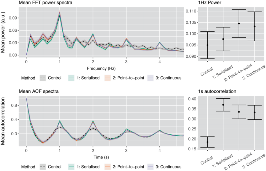
Results of these analyses are shown in Figure 21.2. The gain in spectral power shown in the upper panel at 1 Hz appears modest for all three conditions with a small advantage for the latter two, less destructive, methods. The frequency spectrum also shows peaks for all three retimings at harmonic frequencies of 2, 3, and 4 Hz. The difference between control and retimings is more apparent in the autocorrelation analysis shown in the lower panel. Here, there may be a slight advantage to the first method.Footnote 2
Periodicity and recurrence spectra.
Left: FFT and ACF spectra of the original amplitude envelope and amplitude envelopes resulting from each of the three retimings. Ribbons indicate +/− 1.96 SE. Right: View of only the 1 Hz and one-second peak heights with error bars showing the same confidence interval as ribbons.
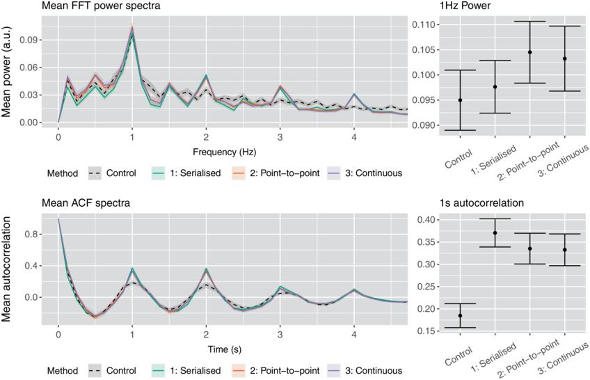
Figure 21.2 Long description
Top: A line graph of mean power versus frequency. It plots overlapping and fluctuating lines for control, serialized, point to point and continuous. The lines show peaks at 1, 2, 3, and 4 Hertz. To its right, an error bar graph plots the mean power, which are as follows. Control, 0.095. Serialized, 0.097. Point to Point, 0.105. Continuous, 0.103. Bottom. A line graph of mean autocorrelation versus time. It plots overlapping and fluctuating lines for control, serialized, point to point, and continuous. The lines show peaks at 1, 2, 3, and 4 seconds. To its right, an error bar graph plots the mean power, which are as follows. Control, 0.17. Serialized, 0.037. Point to Point, 0.33. Continuous, 0.33. The values are estimated.
21.2.4 Discussion
Depending on the hypothesis being investigated, the definition of isochrony may vary. For example, if the researcher hypothesises that the oscillatory structure of the amplitude envelope will elicit neural entrainment, it would be preferable to demonstrate a cyclical periodic structure in the stimulus. Alternatively, if it was hypothesised that greater regularity of edges in the amplitude envelope would increase the salience of the rhythmic structure, recurrence might be more important than cyclical periodicity.
Method 1 appears to be less appropriate for increasing periodicity. Due to the insertion of silence, any naturally occurring cyclical pattern could be disrupted by the creation of discontinuities. Furthermore, as the speech rate is increased without reducing the duration of the utterance, any existing periodicity in the envelope would no longer be coherent with the imposed frequency. This may explain the more modest power increase shown in the close-up view of the 1 Hz bin in the upper right of Figure 21.2. For all retimings, power is also increased at the harmonic bins (2, 3, and 4 Hz), as would be expected from a periodic signal, with no evidence of recurrences at time-domain equivalences (0.5, 0.25, or 0.125s) in the ACF spectrum. This again highlights that power at a frequency in an FFT does not necessarily correspond to recurrence at that frequency. In contrast, there appears to be an advantage to the first method over the others in the ACF measure. This may be because all words were increased by the same rate and, therefore, regularities in the original production of the words were retained.
The advantage of methods 2 and 3 in the FFT analysis may not be enough to justify their selection over method 1. Similarly, their disadvantage compared to method 1 in the ACF analysis may not be enough to justify selection of method 1. The clearer difference is apparent in the warp path cost measure. Both of these measures have lower median values than the lower bound of the 95% HDCI for method 1. This is unsurprising, particularly in the case of method 2, as it defines the shortest path passing through the required anchors. The additional cost of the third method appears to be minimal except with a higher upper bound. This would suggest that more careful checking of outliers may be required.
The results presented here may not necessarily generalise to other stimulus sets. Consider that neither point-to-point nor continuous retiming methods would alter an already isochronous stimulus item, while the serialisation method would insert silences. By extension, the measures reported here capture not only the performance of the retiming method but also the irregularity of speech in the source recording.
21.3 Rhythmic Chimeras
The flexibility of continuous retiming demonstrated in method 3 makes it useful for many applications beyond creating isochronous speech. In natural speech the temporal structure varies in subtle ways that would be challenging to define a priori. Two utterances could consist of the same sequence of words and phrase structure, but the rhythmic structure may vary between speakers or settings.
This section shows how continuous retiming can be used to create a rhythmic chimera. The analogy of a chimera is borrowed here from the term auditory chimera used by Smith et al. (Reference Smith, Delgutte and Oxenham2002) to refer to combining the fine detail of one auditory signal with the amplitude envelope of another to create a hybrid of the two. Here, the rhythmic chimera does not replace the amplitude envelope but instead uses it as a reference to warp the rhythmic structure of one utterance to that of another.
21.3.1 Materials
Example utterances were taken from the CHAINS corpus (Cummins et al., Reference Cummins, Grimaldi, Leonard and Simko2006). This corpus was created to support speaker identification research and consists of 36 speakers producing a range of sentences and longer texts under different reading conditions. Here, the solo sentence tasks were used where the speakers read the sentences at their own pace. Recordings of a male and a female speaker, each producing the same sentence, were sampled from these sentences to demonstrate the creation of rhythmic chimeras.
21.3.2 Method
There are three steps to the creation of a rhythmic chimera. These are feature extraction, alignment, and retiming. A vignette of the full stimulus creation process using R is provided in the supplementary repository (Beith et al., Reference Beith, Barr and Smith2024).
21.3.2.1 Feature Extraction
The first step is to produce time series of each of the signals. The simplest option would be to use the amplitude envelope as with the previous examples. However, an improved alignment can be achieved by using a multivariate signal.
Mel-frequency cepstral coefficients (MFCCs) have been used to perform alignments of utterances in previous studies (e.g., Cummins, Reference Cummins2009) and are used extensively in automatic speech recognition (ASR) tools (e.g., Young et al., Reference Young, Evermann and Gales2015; McAuliffe et al., Reference McAuliffe, Socolof, Mihuc, Wagner and Sonderegger2017). The advantage of MFCCs is that they reduce the feature representation from a full spectrogram to a smaller number (12 in the examples mentioned) of dimensions. More recent ASR tools such as OpenAI’s Whisper (Aldarmaki et al., Reference Aldarmaki, Ullah, Ram and Zaki2022) use full mel-spectrograms. Following this approach, mel-spectrograms with 80 bins and 10 ms time steps (i.e., 100 Hz sampling frequency) were used for feature extraction. As the mel-spectrogram is an intermediate step of MFCC extraction, the melfcc function from the tuneR package (Ligges et al., Reference Ligges, Krey, Mersmann and Schnackenberg2023) was adapted for this purpose.
21.3.2.2 Alignment
Following feature extraction, alignment was performed by dynamic time warping (DTW) using the dtw package (Giorgino, Reference Giorgino2009). The warp paths shown in Figure 21.1 are similar to those that would be obtained from a DTW analysis. Each point in one time series refers to a matched point in the other time series. For DTW, this is done by finding the optimal path through the distance matrix of two signals that meets the defined parameters. When using a multivariate signal such as an MFCC or a mel-spectrogram, the distance method must be specified as “Manhattan.”
As demonstrated by the retiming methods in this chapter, there are many warp paths that can produce similar results. In DTW, paths can be subjected to local constraints to specify particular characteristics. As the intention here is to use the alignment to perform a retiming of the signal, the alignment should be usable as anchor points, preferably with minimal additional processing. Therefore, the alignment path between the two signals must be monotonically increasing.
This constraint can be achieved by specifying a step pattern. An extensive review of step pattern options is included in Rabiner and Juang (Reference Rabiner and Juang1993), and further documentation of options is available in the companion paper for the dtw package (Giorgino, Reference Giorgino2009). Although all step patterns are monotonically non-decreasing, many patterns, as with the serialisation approach (method 1), allow sequential points in one signal to be mapped to the same points in the other signal. Effectively, this would require the insertion of silence or the omission of part of the signal to implement. The Rabiner–Juang Type III step pattern (Rabiner and Juang, Reference Rabiner and Juang1993, Section 4.7) was used here to produce a monotonically increasing alignment. With this pattern, each step taken in one time series must correspond to one or two steps in the other time series.
21.3.2.3 Retiming
The alignment maps points in the mel-spectrogram of one signal to the corresponding points in the mel-spectrogram of the other signal. Therefore, the only step required to produce anchor points for a retiming is to rescale the alignment to the sampling frequency of the signal. Simply reversing the anchors allows for the retiming to be performed in the opposite direction.
This retiming would be useful if the intention was to retime one speaker to have the rhythmic structure of another. A further possibility is to produce ambiguous rhythmic chimeras. This can be done by averaging the anchor points to create a series of anchors representing the midpoint between the time a sound occurs in one speaker’s utterance and the time it occurs in the other speaker’s utterance. For example, if speaker A produces a sound at the time of 500 ms and speaker B produces that same sound at 1,000 ms, both recordings could be altered so that both speakers produce the same sound at 750 ms. The same principle could be extended to produce a continuum of rhythmic structures by weighting the averages.
The vignette provides examples of unaltered recordings of the two speakers and all combinations of full rhythmic chimeras and half-warped rhythmic chimeras. A final example places the two half-warped rhythmic chimeras in left and right channels of a stereo audio file to allow for aural inspection of the alignments.
21.3.3 Results
Rhythmic chimeras are achieved by using DTW both as a means of analysis and of producing the stimulus. Therefore, insofar as DTW is an appropriate means of analysis, the retiming is perfect. Furthermore, criticisms of the retiming could be addressed by altering the parameters (most likely the step pattern) of the DTW analysis.
The primary limitation is that more extreme differences between speakers’ rhythms will result in more disruption in the retimed signal. Where suitable to the experimental paradigm, the half-warped retiming presented here would be an appropriate method of minimising disruption. A further option would be to add additional constraints to the DTW step pattern. In the examples, type “a” slope weighting was used, incurring no additional cost for steps with steeper or shallower slopes. However, weighted slopes could be used to prefer unwarped steps at the local level over steeper or shallower slopes that provide a better fit. A global constraint can also be applied via a windowing function to prevent large deviations from the original signal.
21.4 Discussion
This chapter set out to demonstrate three methods available to researchers for producing stimulus items where temporal structure needs to be controlled or manipulated. To the extent that they were able to produce isochronous speech, all three methods performed well. By design, they ensured that the timing of the p-centre estimate occurred at the intended time. This was demonstrated by increased autocorrelation at the intended period in the time domain (ACF) analysis. When measured in the frequency domain (FFT), the increase in periodicity was less apparent, but with a potential benefit of point-to-point and continuous retiming over control and serialisation.
A limitation of the isochronous stimulus examples is that the speech used was initially produced with quasi-isochronous rhythm and with silences between words. It should not be assumed that these results would generalise to connected speech where a weaker relationship between periodicity in the amplitude envelope and syllable rate would be expected (Zhang et al., Reference Zhang, Zou and Ding2023). In these cases, segmentation will be more challenging and the effects of retiming methods should be assessed for suitability. Furthermore, as found by Aubanel et al. (Reference Aubanel, Davis and Kim2016), imposing strict regularity on speech with complex temporal structure can reduce intelligibility.
There are certain constraints that cannot be changed when altering the temporal structure of speech. Most crucially, information in the speech signal increases monotonically over time, and any transformation would be expected to be monotonically non-decreasing at a minimum. Or, more simply, it is unlikely that a researcher would want any part of the speech to be played backwards. The serialisation method for producing isochronous speech exemplifies one extreme of this limit, where silences are inserted reducing the rate at which the signal progresses to zero. In contrast, the point-to-point method minimises deviation from the rate of the source signal to produce the most efficient path that passes through the desired points. Finally, the continuous retiming method attempts to smooth transitions at rate changes.
For the purposes of this chapter, it is assumed that minimising disruption of temporal structure will in turn minimise disruption of existing prosodic structure. This is reflected in the choice of quantitative measures used to operationalise prosodic disruption. However, future research could benefit from expanding this scope to include qualitative and perceptual measures of prosodic structure.
A potential disadvantage of expressing these methods as warp paths is that it obfuscates some of the more intuitive differences. An equivalence of method 1 could be achieved by simply presenting individual words at predefined times. When constructing a stimulus item in this way, there may be no expectation that the item will sound like a natural utterance or even that it should have the grammatical structure of a sentence or phrase. There are cases where stimuli of this type will have value, such as the design adopted by Quené and Port (Reference Quené and Port2005) where effects of different timings of word presentation were compared. However, caution should be exercised if there is any intention to interpret findings as being generalisable to spontaneous connected speech (see Alexandrou et al., Reference Alexandrou, Saarinen, Kujala and Salmelin2020, for discussion).
Choosing to focus on the commonalities of each of the three retiming methods highlights the complementary relationship between retiming and DTW. While retiming is used for performing manipulations and DTW is used for analysis, both techniques can be expressed as a warp path. An accurate DTW analysis of a source signal and its retiming will result in a warp path resembling the anchor points used to perform the retiming. The steps allowed within these paths allow the researcher to meet the specific needs of their study.
In the case of an a priori temporal structure, such as the imposition of isochrony, the warp path maps a limited set of predefined anchors. Nonetheless, each of the three methods demonstrated had different local continuity constraints. In method 1 the angle could be either a diagonal of a fixed slope or vertical. In method 2 the angle of the slope could change, but only at fixed points. In method 3 the angle of the slope could change but the local change in angle was constrained by the effect it would have on the surrounding points. Recognising this relationship between retiming and DTW provides the stimulus designer with valuable insights from the DTW and speech recognition literature.
While isochrony provides a useful example, a researcher may not always be able to explicitly define the desired anchors in this way. Rhythmic chimeras provide an example of a more flexible approach to retiming a signal. In the example provided, a rhythmic chimera can be used to present one speaker’s utterance with another speaker’s temporal structure. This does not require the researcher to define the temporal structure a priori in terms of onsets or boundaries, yet it allows for a meaningful retiming.
Thus, the approach is valuable for exploring the contribution of temporal organisation to recognition of individual voices (Kello, Reference Kello2003) and accents (Mareüil and Vieru-Dimulescu, Reference Mareüil and Vieru-Dimulescu2006; Kolly et al., Reference Kolly, De Mareüil, Leemann and Dellwo2017; Smith and Rathcke, Reference Smith and Rathcke2017). Furthermore, the half-warped rhythmic chimera would have applications in experimental control of items. Multiple speakers with different voice qualities or realisations of segments could be presented as stimulus items with the same temporal structure. Overall, DTW-based methods offer a flexible and practical way to apply the temporal organisation of one utterance to the spectral structure of another, such as in situations where researchers want to explore how temporal cues yield different structural interpretations of the same phonemic content (e.g., different locations of word, morpheme, or prosodic boundaries; Smith and Hawkins, Reference Smith and Hawkins2012; White et al., Reference White, Mattys, Stefansdottir and Jones2015) or where the contribution of speech rate to the perception of segmental, lexical, or larger units is to be explored (e.g., Dilley and Pitt, Reference Dilley and Pitt2010; Reinisch et al., Reference Reinisch, Jesse and McQueen2011). The methods do so without requiring a priori linguistic assumptions, and allowing for straightforward generation of intermediate values, and their advantages in terms of convenience and naturalness can be explored in future research.
21.5 Conclusion
Retiming speech is a convenient and powerful way of investigating effects of rhythm. However, these manipulations degrade and distort the source signal, with the method chosen to perform the retiming impacting on the naturalness of the resulting stimuli. DTW provides an analytical framework to describe the properties of different approaches to retiming. Recognition of this complementary relationship gives the experimenter a greater ability to parametrise stimulus design to meet specific needs of the experiment. In doing so, this opens up new avenues for experimental stimulus creation that could investigate questions about the contribution of temporal structure to speech perception.
Summary
This chapter presents three methods of creating retimed stimuli with specific temporal characteristics. These methods are discussed in terms of how they affect the existing temporal structure of the speech signal. A further example is provided to highlight the versatility of retiming as a stimulus creation technique.
Implications
In bringing together a range of possible approaches to retiming speech, we hope to encourage researchers to think critically about the choices they make when designing speech stimuli with temporal manipulations. Rather than inventing new techniques, we have combined existing, well-documented tools in a way that highlights the available possibilities.
Gains
The methods presented in this chapter have the potential to be applied in a wide range of disciplines. Furthermore, by building on existing open-source tools, researchers and research software engineers can adapt these methods to meet the requirements of a wide range of paradigms.

 Open access