


1. Introduction
Optical and infrared long-baseline interferometry consists in measuring the fringe contrast and phase of interference fringes in the recombined light collected at several telescopes.Footnote a These observables hold information on the celestial object’s spatial properties, often obtained through model fitting.
In spite of strong evidence of correlations in the data, due to redundancy (Monnier Reference Monnier2007, in the case of closure phases), calibration (Perrin Reference Perrin2003), or atmospheric biases acting on all spectral channels in the same way (Lawson Reference Lawson2000), only a few authors (Perrin et al. Reference Perrin, Ridgway, Coudé du Foresto, Mennesson, Traub and Lacasse2004; Absil et al. Reference Absil2006; Berger et al. Reference Berger2006; Lachaume et al. Reference Lachaume, Rabus, Jordán, Brahm, Boyajian, von Braun and Berger2019; Kammerer et al. Reference Kammerer, Mérand, Ireland and Lacour2020) have accounted for these correlations while most assumed statistically independent errors. In particular, the only interferometric instrument I know of with a data processing software taking into account one source of correlations—calibration—is FLUORFootnote b (at IOTA,Footnote c then CHARA,Footnote d Perrin et al. Reference Perrin, Ridgway, Coudé du Foresto, Mennesson, Traub and Lacasse2004). None of the five first and second-generation ones at the VLTIFootnote e does (Millour et al. Reference Millour, Valat, Petrov and Vannier2008; Hummel & Percheron Reference Hummel and Percheron2006; Le Bouquin et al. Reference Le Bouquin2011; ESO GRAVITY Pipeline Team 2020; ESO MATISSE Pipeline Team 2020). The same lack of support for correlations is present in image reconstruction programmes (e.g. MIRA, see Thiébaut Reference Thiébaut2008), model-fitting tools (e.g. Litpro, see Tallon-Bosc et al. Reference Tallon-Bosc2008), or the still widespread first version of the Optical Interferometric FITS format (OIFITS v. 1, Pauls et al. Reference Pauls, Young, Cotton and Monnier2005).
Unfortunately, ignoring correlations may lead to significant errors in model parameters as Lachaume et al. (Reference Lachaume, Rabus, Jordán, Brahm, Boyajian, von Braun and Berger2019) evidenced with stellar diameters using PIONIERFootnote f (Le Bouquin et al. Reference Le Bouquin2011) data at the VLTI. Also Kammerer et al. (Reference Kammerer, Mérand, Ireland and Lacour2020) established that accounting for correlations is necessary to achieve a higher contrast ratio in companion detection using GRAVITY (Eisenhauer et al. Reference Eisenhauer2011) at the VLTI.
Several sources of correlated uncertainties occur in a multiplicative context, when several data points are normalised with the transfer function (Perrin Reference Perrin2003) or the coherent fluxes are derived with the pixel-to-visibility matrix formalism (Tatulli et al. Reference Tatulli2007). In both cases, the uncertainty on the multiplicative factor translates into a systematic, correlated one in the final data product. In the context of experimental nuclear physics, Peelle (Reference Peelle1987) noted that this scenario could lead to an estimate falling below the individual data points, a paradox known as Peelle’s Pertinent Puzzle (PPP). It results from the usual, but actually incorrect, way to propagate covariances, in which the measured values are used in the calculations (D’Agostini Reference D’Agostini1994; Neudecker, Frühwirth, & Leeb Reference Neudecker, Frühwirth and Leeb2012). A few workarounds have been proposed but they are either computationally expensive (e.g. sampling of the posterior probability distribution for Bayesian analysis, see Neudecker et al. Reference Neudecker, Frühwirth and Leeb2012) or require a conceptually difficult implementation (Becker et al. Reference Becker2012; Nisius Reference Nisius2014).
The issue, however, is not widely known in many other fields where the problem has seldom arisen. In this paper, I present the paradox within the context of long-baseline interferometry (Section 2), derive the order of magnitude of its effect using the modelling of a single value (Section 3), analyse in detail its effect in least squares model fitting (Section 4), and propose a simple, computer-efficient way to avoid it (Section 5).
2. Peelle’s pertinent puzzle
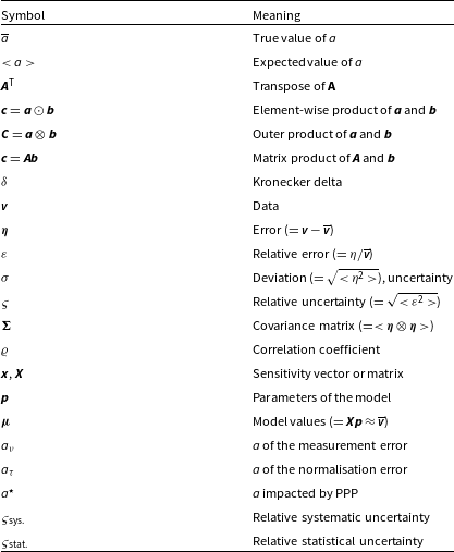
I rewrite and adapt Peelle’s original example in the context of long-baseline interferometry (see Neudecker et al. Reference Neudecker, Frühwirth and Leeb2012, Sections 1 and 2.1). The mathematical symbols used in this article are summarised in Table 1. One or several calibrator observations yield the inverse of the instrumental fringe contrast
 $\tau \pm \tau\varsigma_{\tau}$
. I use the relative uncertainty
$\tau \pm \tau\varsigma_{\tau}$
. I use the relative uncertainty
 $\varsigma_{\tau}$
on the transfer function as it is often referred to in percentage terms. A visibility amplitude is now estimated from two contrast measurements
$\varsigma_{\tau}$
on the transfer function as it is often referred to in percentage terms. A visibility amplitude is now estimated from two contrast measurements
 $\nu_1 \pm \sigma_{\nu}$
and
$\nu_1 \pm \sigma_{\nu}$
and
 $\nu_2 \pm \sigma_{\nu}$
. For each measurement, the visibility amplitudes are
$\nu_2 \pm \sigma_{\nu}$
. For each measurement, the visibility amplitudes are
 \begin{align} {{\scriptstyle V}}_1 &= {\tau\nu_1}\pm{\tau\sigma_{\nu}}\left({\pm\tau\nu_1\varsigma_{\tau}}\right),\end{align}
 \begin{align} {\scriptstyle V}_2 &= {\tau\nu_2}\pm{\tau\sigma_{\nu}}\left({\pm\tau\nu_2\varsigma_{\tau}}\right),\end{align}
where the second-order error term
 $\tau\varsigma_{\tau}\sigma_{\nu}$
has been ignored.
$\tau\varsigma_{\tau}\sigma_{\nu}$
has been ignored.
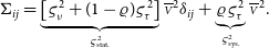
They are normalised with the same quantity (
 $\tau$
), so they are correlated, hence the systematic uncertainty term between parentheses in Eq. (1). Error propagation yields the covariance matrix:
$\tau$
), so they are correlated, hence the systematic uncertainty term between parentheses in Eq. (1). Error propagation yields the covariance matrix:
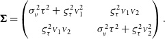 \begin{equation} {\boldsymbol\Sigma} = \begin{pmatrix} \sigma_{\nu}^2\tau^2 + \varsigma_{\tau}^2{{\scriptstyle V}}_1^2 &\quad \varsigma_{\tau}^2{{\scriptstyle V}}_1{{\scriptstyle V}}_2\\ \varsigma_{\tau}^2{{\scriptstyle V}}_1{{\scriptstyle V}}_2 &\quad \sigma_{\nu}^2\tau^2 + \varsigma_{\tau}^2{{\scriptstyle V}}_2^2 \end{pmatrix}.\end{equation}
Under the hypothesis of Gaussian errors, I obtain the least squares estimate using the weight matrix
 $${\bf{\it W}} = {{\bf{\Sigma }}^{ - 1}}$$
:
$${\bf{\it W}} = {{\bf{\Sigma }}^{ - 1}}$$
:
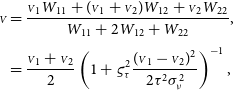 \begin{gather}\begin{split} {\scriptstyle V} &= \frac{ {{\scriptstyle V}}_1 W_{11} + ({{\scriptstyle V}}_1 + {{\scriptstyle V}}_2) W_{12} + {{\scriptstyle V}}_2 W_{22} } { W_{11} + 2 W_{12} + W_{22} }, \\[3pt] &= \frac{{{\scriptstyle V}}_1 + {{\scriptstyle V}}_2}{2} \left(1 + \varsigma_{\tau}^2\frac{({{\scriptstyle V}}_1-{{\scriptstyle V}}_2)^2}{2\tau^2\sigma_{\nu}^2}\right)^{-1},\end{split} \end{gather}
with the uncertainty:
 \begin{align} {\sigma^{2}_{{\scriptstyle V}}} &= \frac{1}{W_{11} + 2W_{12} + W_{22}},\nonumber\\[3pt] &= \left[ \left(\frac{\tau\sigma_{\nu}}{\sqrt{2}}\right)^2 + \frac{{{\scriptstyle V}}_1^2 + {{\scriptstyle V}}_2^2}{2}\varsigma_{\tau}^2 \right] \frac{2{{\scriptstyle V}}}{{{\scriptstyle V}}_1 + {{\scriptstyle V}}_2}.\end{align}
The visibility estimate
 ${{\scriptstyle V}}$
systematically falls below the average of the two values
${{\scriptstyle V}}$
systematically falls below the average of the two values
 ${{\scriptstyle V}}_1$
and
${{\scriptstyle V}}_1$
and
 ${{\scriptstyle V}}_2$
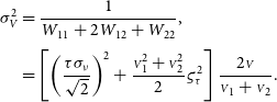
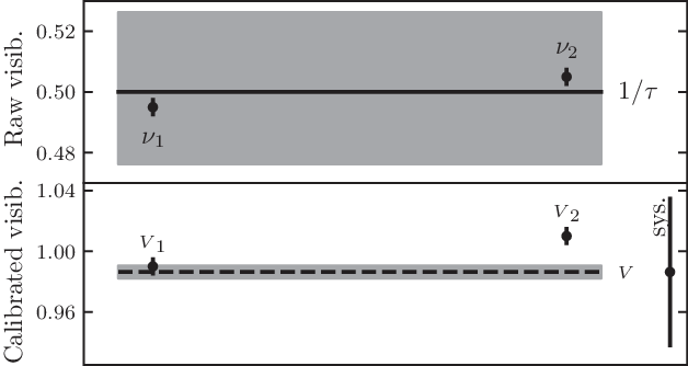
. If the measurements differ significantly, it can even fall below the lowest value. Figure 1 gives such an example with an instrumental visibility of 50% and two measurements on an unresolved target:
${{\scriptstyle V}}_2$
. If the measurements differ significantly, it can even fall below the lowest value. Figure 1 gives such an example with an instrumental visibility of 50% and two measurements on an unresolved target:
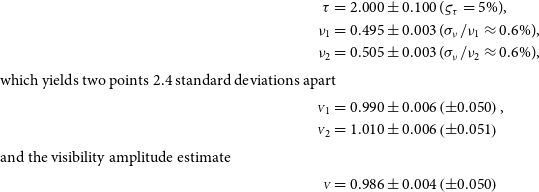 \begin{align*} \tau &= 2.000 \pm 0.100\ (\varsigma_{\tau} = 5\%),\\ \nu_1 &= 0.495 \pm 0.003\ (\sigma_{\nu}/\nu_1 \approx 0.6\%),\\ \nu_2 &= 0.505 \pm 0.003\ (\sigma_{\nu}/\nu_2 \approx 0.6\%),\\{\rm {which\,yields\,two\,points\,2.4\,standard\,deviations\,apart}}\\{{\scriptstyle V}}_1 &= {0.990}\pm{0.006}\left(\pm{0.050}\right),\\ {{\scriptstyle V}}_2 &= {1.010}\pm{0.006}\left({\pm 0.051}\right)\\{\rm {and\,the\,visibility\,amplitude\,estimate}}\\{{\scriptstyle V}} &= {0.986}\pm{0.004}\left(\pm{0.050}\right)\end{align*}
falls outside the data range. The uncertainties quoted for
 ${{\scriptstyle V}}$
correspond to the first and second terms within the square brackets of Eq. (4).
${{\scriptstyle V}}$
correspond to the first and second terms within the square brackets of Eq. (4).
Symbols used in this paper. Lower case bold font is used for vectors and upper case bold font for matrices.
Original Peelle problem rewritten in the context of interferometry. Top: Two raw visibility amplitudes
 $\nu_1$
and
$\nu_1$
and
 $\nu_2$
(points with statistic error bars of
$\nu_2$
(points with statistic error bars of
 $\approx 0.6\%$
) are calibrated by the transfer function
$\approx 0.6\%$
) are calibrated by the transfer function
 $1/\tau$
(solid line with systematic error zone of 5%). Bottom: the two calibrated visibility measurements
$1/\tau$
(solid line with systematic error zone of 5%). Bottom: the two calibrated visibility measurements
 ${{\scriptstyle V}}_1$
and
${{\scriptstyle V}}_1$
and
 ${{\scriptstyle V}}_2$
(points with statistic error bars of
${{\scriptstyle V}}_2$
(points with statistic error bars of
 $\approx 0.6\%$
) are strongly correlated. The least squares estimate for the visibility
$\approx 0.6\%$
) are strongly correlated. The least squares estimate for the visibility
 ${{\scriptstyle V}}$
(dashed line, with statistic uncertainty error zone displayed) falls outside of the data range. The systematic error on
${{\scriptstyle V}}$
(dashed line, with statistic uncertainty error zone displayed) falls outside of the data range. The systematic error on
 ${{\scriptstyle V}}$
,
${{\scriptstyle V}}$
,
 ${{\scriptstyle V}}_1$
, and
${{\scriptstyle V}}_1$
, and
 ${{\scriptstyle V}}_2$
is shown on the right.
${{\scriptstyle V}}_2$
is shown on the right.
3. Fit by a constant
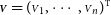
I now generalise the results of the last section to an arbitrary number of measurements of a single normalised quantity, such as the visibility amplitude of an unresolved source, which is expected to be constantly one for all interferometric baselines. Let the column vector
 ${\scriptstyle{\bf{\rm{V}}}} = {({{\scriptstyle V}}_1, \cdots, {{\scriptstyle V}}_n)^{{T}}}$
contain the n visibility amplitudes. It is derived from an uncalibrated quantity like the fringe contrast,
${\scriptstyle{\bf{\rm{V}}}} = {({{\scriptstyle V}}_1, \cdots, {{\scriptstyle V}}_n)^{{T}}}$
contain the n visibility amplitudes. It is derived from an uncalibrated quantity like the fringe contrast,
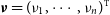 $\boldsymbol{\nu} = {(\nu_1, \cdots, \nu_n)^{{T}}}$
and a normalisation factor, like the cotransfer function,
$\boldsymbol{\nu} = {(\nu_1, \cdots, \nu_n)^{{T}}}$
and a normalisation factor, like the cotransfer function,
 $\boldsymbol{\tau} = {(\tau_1, \cdots, \tau_n)^{{T}}}$
by
$\boldsymbol{\tau} = {(\tau_1, \cdots, \tau_n)^{{T}}}$
by
 \begin{equation} {\scriptstyle{\bf{\it{V}}}} = \boldsymbol{\tau}\odot\boldsymbol{\nu},\end{equation}
where
 $\odot$
denotes the Hadamard (element-wise) product of vectors. With
$\odot$
denotes the Hadamard (element-wise) product of vectors. With
 $\overline{\scriptstyle V}$
,
$\overline{\scriptstyle V}$
,
 $\overline{\tau}$
, and
$\overline{\tau}$
, and
 $\overline{\nu}$
the true, but unknown, values of these quantities, the error vector on
$\overline{\nu}$
the true, but unknown, values of these quantities, the error vector on
 ${\scriptstyle{\bf{\it{V}}}}$
:
${\scriptstyle{\bf{\it{V}}}}$
:
 \begin{align} {\boldsymbol\eta} &= {\scriptstyle{\bf{\it{V}}}} - \overline{\scriptstyle V}, \end{align}
can be written as a sum of measurement and normalisation relative errors if one ignores the second-order terms:
 \begin{align} {\boldsymbol\eta} &= (\boldsymbol\varepsilon_{\boldsymbol{\nu}} + \boldsymbol\varepsilon_{\boldsymbol\tau}) \overline{\scriptstyle V}.\end{align}
These errors are given by:
 \begin{align}\boldsymbol\varepsilon_{\boldsymbol{\nu}} &= \frac{1}{\overline{\nu}} (\boldsymbol{\nu} - \overline{\nu}), \end{align}
 \begin{align} {\boldsymbol\varepsilon}_{\boldsymbol\tau} &= \frac{1}{\overline{\tau}} ({\boldsymbol{\tau}}-{\overline{\tau}}).\end{align}
I assume
 $\boldsymbol\varepsilon_{\boldsymbol\nu}$
and
$\boldsymbol\varepsilon_{\boldsymbol\nu}$
and
 ${\boldsymbol\varepsilon}_{\boldsymbol\tau}$
are independent, of mean 0, and have standard deviations
${\boldsymbol\varepsilon}_{\boldsymbol\tau}$
are independent, of mean 0, and have standard deviations
 $\varsigma_{\nu}$
and
$\varsigma_{\nu}$
and
 $\varsigma_{\tau}$
, respectively. In addition, I consider correlation of the normalisation errors, with correlation coefficient
$\varsigma_{\tau}$
, respectively. In addition, I consider correlation of the normalisation errors, with correlation coefficient
 $\varrho$
. In the case of interferometry, it can arise from the uncertainty on the calibrators’ geometry. The covariance matrix of the visibility amplitudes is given by:
$\varrho$
. In the case of interferometry, it can arise from the uncertainty on the calibrators’ geometry. The covariance matrix of the visibility amplitudes is given by:
 \begin{align} {\boldsymbol\Sigma} &= <{{\boldsymbol\eta}\otimes{\boldsymbol\eta}}>,\end{align}
where
 $\otimes$
denotes the outer product of vectors and
$\otimes$
denotes the outer product of vectors and
 $<>$
stands for the expected value, so that
$<>$
stands for the expected value, so that
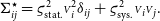
 \begin{align}\Sigma_{ij} &= \underbrace{\left[ \varsigma_{\nu}^2 + (1-\varrho)\varsigma_{\tau}^2 \right]}_{{\varsigma_{\text{stat.}}^2}} \overline{\scriptstyle V}^2 \delta_{ij} + \underbrace{\varrho\varsigma_{\tau}^2}_{{\varsigma_{\text{sys.}}^2}} \overline{\scriptstyle V}^2.\end{align}
The non-diagonal diagonal elements of the matrix feature the systematic relative uncertainty
 ${\varsigma_{\text{sys.}}}$
, that is, the correlated component of the uncertainties. In the case of a fully correlated transfer function (
${\varsigma_{\text{sys.}}}$
, that is, the correlated component of the uncertainties. In the case of a fully correlated transfer function (
 $\varrho =1$
), it is equal its uncertainty (
$\varrho =1$
), it is equal its uncertainty (
 ${\varsigma_{\text{sys.}}} = \varsigma_{\tau}$
). The diagonal term of the matrix additionally includes the statistical relative uncertainty
${\varsigma_{\text{sys.}}} = \varsigma_{\tau}$
). The diagonal term of the matrix additionally includes the statistical relative uncertainty
 ${\varsigma_{\text{stat.}}}$
, that is, the uncorrelated component of the uncertainties. In the case of a fully correlated transfer function, it is equal to the uncertainty of the uncalibrated visibility (
${\varsigma_{\text{stat.}}}$
, that is, the uncorrelated component of the uncertainties. In the case of a fully correlated transfer function, it is equal to the uncertainty of the uncalibrated visibility (
 ${\varsigma_{\text{stat.}}} = \varsigma_{\nu}$
).
${\varsigma_{\text{stat.}}} = \varsigma_{\nu}$
).
The value
 $\overline{\scriptstyle V}$
is yet to be determined, so the covariances are often derived using the measurements
$\overline{\scriptstyle V}$
is yet to be determined, so the covariances are often derived using the measurements
 ${\scriptstyle{\bf{\it{V}}}}$
in the propagation:
${\scriptstyle{\bf{\it{V}}}}$
in the propagation:
 \begin{equation} {\Sigma^{\star}_{ij}} = {\varsigma_{\text{stat.}}^2} {\scriptstyle V}_i^2 \delta_{ij} + {\varsigma_{\text{sys.}}^2}{\scriptstyle V}_i{\scriptstyle V}_j.\end{equation}
The least squares estimate for
 $\overline{\scriptstyle V}$
is given by:
$\overline{\scriptstyle V}$
is given by:
 \begin{equation} {\mu}^{\star} = \frac {\bf{\it{x}}^{\text{T}}{\boldsymbol\Sigma}^{\star-1}{\scriptstyle{\bf{\it{V}}}}}{\bf{\it{x}}^{\text{T}}\boldsymbol\Sigma^{\star-1}\bf{\it{x}}}\end{equation}
where
 $\bf{\it{x}} = {(1, \cdots, 1)^{\text{T}}}$
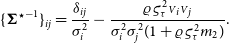
is the trivial sensitivity vector. The covariance matrix is the sum of an invertible diagonal matrix and one of rank one—see (12)—, so that the inverse is obtained using the Woodbury matrix identity:
$\bf{\it{x}} = {(1, \cdots, 1)^{\text{T}}}$
is the trivial sensitivity vector. The covariance matrix is the sum of an invertible diagonal matrix and one of rank one—see (12)—, so that the inverse is obtained using the Woodbury matrix identity:
 \begin{align} \{{{\boldsymbol\Sigma}^{\star}}^{-1}\}_{ij} &= \frac{\delta_{ij}}{{\sigma}_i^2} - \frac{{\varsigma_{\text{sys.}}^2}{{\scriptstyle V}}_i{{\scriptstyle V}}_j} {{\sigma}_i^2{\sigma}_j^2\Big(1 + {\varsigma_{\text{sys.}}^2}\sum\limits_{k} \frac{{{\scriptstyle V}}_k^2}{{\sigma}_k^2}\Big)}, \end{align}
where we have introduced the statistical (uncorrelated) component of the uncertainty on the calibrated visibilities:
 \begin{align} {\sigma}_i &= {\varsigma_{\text{stat.}}}{{\scriptstyle V}}_i .\end{align}
Appendix A.1 shows the analytical derivation for the least squares estimate
 ${\mu}^{\star}$
using the previous formulae. I write it in a way that highlights the generalisation of Eq. (3) of the previous section:
${\mu}^{\star}$
using the previous formulae. I write it in a way that highlights the generalisation of Eq. (3) of the previous section:
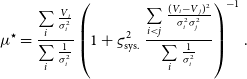 \begin{equation} {\mu}^{\star} = \frac{\sum\limits_{i} \frac{{\scriptstyle V}_i}{{\sigma}_i^2}}{\sum\limits_i \frac{1}{{\sigma}_i^2}} \left( 1 + {\varsigma_{\text{sys.}}^2}\,\frac {\sum\limits_{i<j} \frac{({\scriptstyle V}_i-{\scriptstyle V}_j)^2}{{\sigma}_i^2{\sigma}_j^2}} {\sum\limits_i \frac{1}{{\sigma}_i^2}} \right)^{-1}.\end{equation}
For small enough errors (
 ${\eta}_i \ll \overline{\scriptstyle V}$
), the second-order Taylor development in
${\eta}_i \ll \overline{\scriptstyle V}$
), the second-order Taylor development in
 ${\eta}_i = {\scriptstyle V}_i - \overline{\scriptstyle V}$
yields (see Appendix A.2):
${\eta}_i = {\scriptstyle V}_i - \overline{\scriptstyle V}$
yields (see Appendix A.2):
 \begin{equation} {\mu}^{\star} \approx \overline{\scriptstyle V} + \frac1n {\sum\limits_i {\eta}_i} - \frac{1}{\overline{\scriptstyle V}} \left(\frac1{2n}\frac{{\varsigma_{\text{sys.}}^2}}{{\varsigma_{\text{stat.}}^2}} + \frac 1{n^2}\right) \sum\limits_{i\ne j} ({\eta}_i-{\eta}_j)^2.\end{equation}
Since
 $<{{\eta}_i}> = 0$
and
$<{{\eta}_i}> = 0$
and
 $<{({\eta}_i-{\eta}_j)^2}> = 2{\varsigma_{\text{stat.}}^2}\overline{\scriptstyle V}^2$
, the expected value:
$<{({\eta}_i-{\eta}_j)^2}> = 2{\varsigma_{\text{stat.}}^2}\overline{\scriptstyle V}^2$
, the expected value:
 \begin{equation} <{{\mu}^{\star}}> \approx \overline{\scriptstyle V} \left[ 1 - \left(1-\frac1n\right) \left(2{\varsigma_{\text{stat.}}^2} + n{\varsigma_{\text{sys.}}^2}\right) \right]\end{equation}
is biased. If the data are not correlated (
 ${\varsigma_{\text{sys.}}} = 0$
), the bias is small (
${\varsigma_{\text{sys.}}} = 0$
), the bias is small (
 ${\varsigma_{\text{stat.}}^2}$
to
${\varsigma_{\text{stat.}}^2}$
to
 $2{\varsigma_{\text{stat.}}^2}$
) but it becomes larger for correlated data if the number of points is large (
$2{\varsigma_{\text{stat.}}^2}$
) but it becomes larger for correlated data if the number of points is large (
 $n/2$
to
$n/2$
to
 $n \times \varsigma_{\tau}^2$
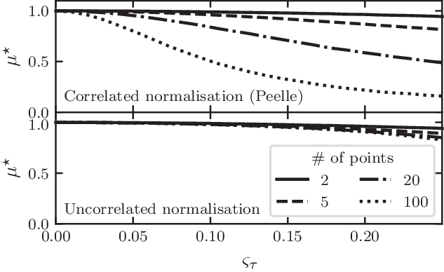
for fully correlated data) as D’Agostini (Reference D’Agostini1994) already noted. This analytical derivation confirms the numerical simulation by (Neudecker et al. Reference Neudecker, Frühwirth and Leeb2012, see their Figure 4). For visualisation purposes, Figure 2 shows a similar simulation of the bias as a function of the normalisation uncertainty
$n \times \varsigma_{\tau}^2$
for fully correlated data) as D’Agostini (Reference D’Agostini1994) already noted. This analytical derivation confirms the numerical simulation by (Neudecker et al. Reference Neudecker, Frühwirth and Leeb2012, see their Figure 4). For visualisation purposes, Figure 2 shows a similar simulation of the bias as a function of the normalisation uncertainty
 $\varsigma_{\tau}$
for various data sizes (
$\varsigma_{\tau}$
for various data sizes (
 $n = 2$
to 100). I have verified that it reproduces the quadratic behaviour of Eq. (18) for small values of
$n = 2$
to 100). I have verified that it reproduces the quadratic behaviour of Eq. (18) for small values of
 ${\varsigma_{\text{stat.}}}$
and
${\varsigma_{\text{stat.}}}$
and
 ${\varsigma_{\text{sys.}}}$
(bias inferior to 10–20% of
${\varsigma_{\text{sys.}}}$
(bias inferior to 10–20% of
 $\overline{\scriptstyle V}$
).
$\overline{\scriptstyle V}$
).
Fit
 $\mu^{\star}$
to unresolved visibilities (
$\mu^{\star}$
to unresolved visibilities (
 ${{\scriptstyle V}} = 1$
), as a function of the relative uncertainty on the calibration
${{\scriptstyle V}} = 1$
), as a function of the relative uncertainty on the calibration
 $\varsigma_{\tau}$
and the number of measurements n.
$\varsigma_{\tau}$
and the number of measurements n.
 $2/n\times10^5$
simulations were made and averaged, assuming that
$2/n\times10^5$
simulations were made and averaged, assuming that
 $\varepsilon_{\nu}$
and
$\varepsilon_{\nu}$
and
 $\varepsilon_{\tau}$
follow normal distributions. Top: fully correlated normalisation like in original Peelle’s puzzle (
$\varepsilon_{\tau}$
follow normal distributions. Top: fully correlated normalisation like in original Peelle’s puzzle (
 $\varsigma_{\nu}=0.02$
and
$\varsigma_{\nu}=0.02$
and
 $\varrho = 1$
). Bottom: normalisation error without correlation (
$\varrho = 1$
). Bottom: normalisation error without correlation (
 $\varsigma_{\nu}=0.02$
and
$\varsigma_{\nu}=0.02$
and
 $\varrho = 0$
).
$\varrho = 0$
).
The bias from PPP arises, intuitively, because the modelled uncertainty is a non-constant function of the measured value. In the present case, data that fall below the average are given a lower uncertainty and, thus, a higher weight in the least squares fit. Conversely, data that fall above the average have a higher uncertainty and a lower weight. This fundamentally biases the estimate towards lower values. The effect is much stronger with correlations because it impacts the
 $\sim n^2/2$
independent elements of the covariance matrix instead of being restricted to the n diagonal ones. In the literature, the puzzle is generally discussed as arising from a normalisation, as it it where it has been first identified. However, I show in Appendix A.3 that it is not necessary and determine the bias in the case of correlated photon noise.
$\sim n^2/2$
independent elements of the covariance matrix instead of being restricted to the n diagonal ones. In the literature, the puzzle is generally discussed as arising from a normalisation, as it it where it has been first identified. However, I show in Appendix A.3 that it is not necessary and determine the bias in the case of correlated photon noise.
For spectro-interferometric observations with four telescopes, the number of correlated points can be over 1 000, so even with a low correlation coefficient, the bias can be significant. For instance, a single GRAVITY observation in medium spectral resolution yields
 $n = 6 \times 210$
visibility amplitudes. With an observed correlation of
$n = 6 \times 210$
visibility amplitudes. With an observed correlation of
 $\varrho \approx 16$
% in the instrumental visibility amplitudes (Kammerer et al. Reference Kammerer, Mérand, Ireland and Lacour2020) and a typical
$\varrho \approx 16$
% in the instrumental visibility amplitudes (Kammerer et al. Reference Kammerer, Mérand, Ireland and Lacour2020) and a typical
 $\varsigma_{\tau} = 1$
–2% normalisation error, the bias on the calibrated visibilities could be 2–8%.
$\varsigma_{\tau} = 1$
–2% normalisation error, the bias on the calibrated visibilities could be 2–8%.
4. General model fitting
I now consider a set of measurements corresponding to the linear model:
 \begin{align} \boldsymbol\mu &= \bf{\it{X}}\bf{\it{p}},\end{align}
where
 $\bf{\it{p}}$
are the unknown parameters and
$\bf{\it{p}}$
are the unknown parameters and
 $\bf{\it{X}}$
is the known sensitivity matrix. Typically,
$\bf{\it{X}}$
is the known sensitivity matrix. Typically,
 $x_{ik}=f_k(u_i, v_i)$
for a linear model and
$x_{ik}=f_k(u_i, v_i)$
for a linear model and
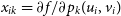 $x_{ik} = \partial f/\partial p_k(u_i, v_i)$
for a non-linear model approximated by a linear one close to a solution. (
$x_{ik} = \partial f/\partial p_k(u_i, v_i)$
for a non-linear model approximated by a linear one close to a solution. (
 $\it{u}, \it{v}$
) is the reduced baseline projected on to the sky, that is,
$\it{u}, \it{v}$
) is the reduced baseline projected on to the sky, that is,
 $u = B_u / \lambda$
if
$u = B_u / \lambda$
if
 $\bf{\it{B}}$
is the baseline and
$\bf{\it{B}}$
is the baseline and
 $\lambda$
, the wavelength. The true values
$\lambda$
, the wavelength. The true values
 $\overline{\scriptstyle{\bf{\it{V}}}}$
are impacted by errors so that the data are
$\overline{\scriptstyle{\bf{\it{V}}}}$
are impacted by errors so that the data are
 \begin{align} {\scriptstyle{\bf{\it{V}}}} &= \overline{\scriptstyle{\bf{\it{V}}}} + {\boldsymbol\eta}\end{align}
with the error term
 ${\boldsymbol\eta}$
again expressed as the sum of a measurement and a normalisation error:
${\boldsymbol\eta}$
again expressed as the sum of a measurement and a normalisation error:
 \begin{align} {\boldsymbol\eta} &= {\boldsymbol\eta_{\boldsymbol\nu}} + \boldsymbol\varepsilon_{\boldsymbol\tau} \odot \overline{\scriptstyle{\bf{\it{V}}}}.\end{align}
The measurement errors
 $\boldsymbol\eta_{\boldsymbol\nu}$
and normalisation errors
$\boldsymbol\eta_{\boldsymbol\nu}$
and normalisation errors
 $\boldsymbol\varepsilon_{\boldsymbol\tau}$
follow multivariate distributions of mean zero with covariance matrices
$\boldsymbol\varepsilon_{\boldsymbol\tau}$
follow multivariate distributions of mean zero with covariance matrices
 ${\boldsymbol\Sigma_{\boldsymbol\nu}}$
and
${\boldsymbol\Sigma_{\boldsymbol\nu}}$
and
 ${\boldsymbol\Sigma_{\boldsymbol\tau}}$
, respectively. Given the covariance matrix
${\boldsymbol\Sigma_{\boldsymbol\tau}}$
, respectively. Given the covariance matrix
 ${\boldsymbol\Sigma}$
of this model, the least squares estimate is
${\boldsymbol\Sigma}$
of this model, the least squares estimate is
 \begin{align} \bf{\it{p}} &= ({\bf{\it{X}}}^{\text{T}} {\boldsymbol\Sigma}^{-1} \bf{\it{X}})^{-1} ({\bf{\it{X}}}^{\text{T}} {\boldsymbol\Sigma}^{-1} {\scriptstyle{\bf{\it{V}}}})\end{align}
I investigate four ways to determine the covariance matrix
 ${\boldsymbol\Sigma}$
-
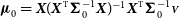
1. Ignoring the correlations in the normalisation using
 ${\boldsymbol\Sigma}_0 = {{\boldsymbol\Sigma}_{\boldsymbol\nu}} + ({\scriptstyle{\bf{\it{V}}}}\otimes{{\scriptstyle{\bf{\it{V}}}}})\odot({{\boldsymbol\Sigma}_{\boldsymbol\tau}}\odot \bf{\it{I}})$
. Let
$\boldsymbol\mu_{0}= \bf{\it{X}}({\bf{\it{X}}}^{\text{T}}{\boldsymbol\Sigma}_0^{-1}\bf{\it{X}})^{-1}{\bf{\it{X}}}^{\text{T}}{\boldsymbol\Sigma}_0^{-1}{\scriptstyle{\bf{\it{V}}}}$
the resulting model of the data.
${\boldsymbol\Sigma}_0 = {{\boldsymbol\Sigma}_{\boldsymbol\nu}} + ({\scriptstyle{\bf{\it{V}}}}\otimes{{\scriptstyle{\bf{\it{V}}}}})\odot({{\boldsymbol\Sigma}_{\boldsymbol\tau}}\odot \bf{\it{I}})$
. Let
$\boldsymbol\mu_{0}= \bf{\it{X}}({\bf{\it{X}}}^{\text{T}}{\boldsymbol\Sigma}_0^{-1}\bf{\it{X}})^{-1}{\bf{\it{X}}}^{\text{T}}{\boldsymbol\Sigma}_0^{-1}{\scriptstyle{\bf{\it{V}}}}$
the resulting model of the data. -
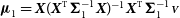
2. Using the nave estimate
${\boldsymbol\Sigma}^{\star} = {\boldsymbol\Sigma_{\boldsymbol\nu}} + ({\scriptstyle{\bf{\it{V}}}}\otimes{\scriptstyle{\bf{\it{V}}}})\odot{\boldsymbol\Sigma_{\boldsymbol\tau}}$
which is known to lead to PPP in the trivial case of a constant model. -
3. Using the data model of the fit without the normalisation error:
${\boldsymbol\Sigma}_1 = {\boldsymbol\Sigma_{\boldsymbol\nu}} + (\boldsymbol\mu_{0}\otimes{\boldsymbol\mu_{0}})\odot{\boldsymbol\Sigma_{\boldsymbol\tau}}$
. This is the generalisation of the two-variable approach by Neudecker et al. (Reference Neudecker, Frühwirth, Kawano and Leeb2014). The resulting least squares model is
${\boldsymbol\mu}_{1} = \bf{\it{X}}({\bf{\it{X}}}^{\text{T}}{\boldsymbol\Sigma}_1^{-1}\bf{\it{X}})^{-1}{\bf{\it{X}}}^{\text{T}}{\boldsymbol\Sigma}_1^{-1}{\scriptstyle{\bf{\it{V}}}}$
. -
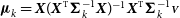
4. Recursively fitting the data by updating the data model in the covariance matrix. I derive
$\boldsymbol\mu_{k} = \bf{\it{X}}({\bf{\it{X}}}^{\text{T}}{\boldsymbol\Sigma}_k^{-1}\bf{\it{X}})^{-1}{\bf{\it{X}}}^{\text{T}}{\boldsymbol\Sigma}_k^{-1}{\scriptstyle{\bf{\it{V}}}}$
using
${\boldsymbol\Sigma}_{k} = {\boldsymbol\Sigma_{\boldsymbol\nu}} + (\boldsymbol\mu_{k-1}\otimes {\boldsymbol\mu}_{k-1})\odot{\boldsymbol\Sigma_{\boldsymbol\tau}}$
, starting with the estimate
${\boldsymbol\mu_{1}}$
(
$k = 2$
).


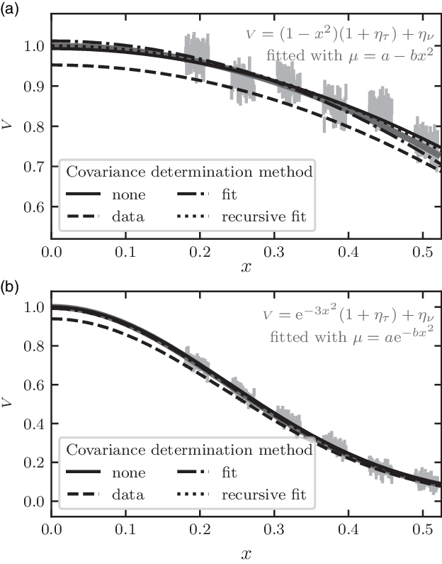
In order to compare these covariance matrix prescriptions, I will use the typical example of an under-resolved centro-symmetric source observed at a four-telescope facility in medium spectral resolution. It is close to the context under which I serendipitiously noticed the effect while modelling stellar diameters (see Lachaume et al. Reference Lachaume, Rabus, Jordán, Brahm, Boyajian, von Braun and Berger2019). The python code to produce the results (figures in this paper) is available on github.Footnote g In the under-resolved case all models—Gaussian, uniform disc, or limb-darkened disc—are equivalent (Lachaume Reference Lachaume2003), so I will use instead a linear least squares fit
 $\mu = a - bx^2$
to
$\mu = a - bx^2$
to
 ${\scriptstyle V} \approx 1 - x^2$
where x is dimensionless variable proportional to the projected baseline length
${\scriptstyle V} \approx 1 - x^2$
where x is dimensionless variable proportional to the projected baseline length
 $\sqrt{u^2+v^2}$
. This fit corresponds to the second-order Taylor development of any of the aforementioned models. Figure 3(a) shows the example of such a fit performed for each covariance matrix prescription. Data have been simulated using
$\sqrt{u^2+v^2}$
. This fit corresponds to the second-order Taylor development of any of the aforementioned models. Figure 3(a) shows the example of such a fit performed for each covariance matrix prescription. Data have been simulated using
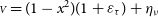 ${\scriptstyle V} = (1-x^2)(1 + \varepsilon_{\tau}) + \eta_{\nu}$
where
${\scriptstyle V} = (1-x^2)(1 + \varepsilon_{\tau}) + \eta_{\nu}$
where
 $\varepsilon_{\tau}$
is a fully correlated normalisation error (3%) and
$\varepsilon_{\tau}$
is a fully correlated normalisation error (3%) and
 $\eta_{\nu}$
are uncorrelated statistical errors (2%). As expected, the use of data
$\eta_{\nu}$
are uncorrelated statistical errors (2%). As expected, the use of data
 ${\scriptstyle{\bf{\it{V}}}}$
in the correlation matrix, method 2, leads to grossly underestimated data values, in the very same way as in the classical Peelle case described in Sections 2 and 3. Other methods, including ignoring correlations, yield reasonable parameter estimates.
${\scriptstyle{\bf{\it{V}}}}$
in the correlation matrix, method 2, leads to grossly underestimated data values, in the very same way as in the classical Peelle case described in Sections 2 and 3. Other methods, including ignoring correlations, yield reasonable parameter estimates.
Model fitting to simulated correlated data from a four-telescope interferometer (6 baselines) with medium spectral resolution (R = 100) with 2% uncorrelated measurement error and 3% correlated normalisation error (light grey points with the measurement error bar). Top: Simulated under-resolved data
 ${\scriptstyle V} = 1-x^2$
(thick grey line) are fitted with linear least squares model
${\scriptstyle V} = 1-x^2$
(thick grey line) are fitted with linear least squares model
 $\mu = a-bx^2$
using the four prescriptions for the covariance matrix. Bottom: The same for well-resolved data
$\mu = a-bx^2$
using the four prescriptions for the covariance matrix. Bottom: The same for well-resolved data
 ${{\scriptstyle V}} = \exp -3x^2$
and non-linear least squares with model
${{\scriptstyle V}} = \exp -3x^2$
and non-linear least squares with model
 $\mu = a\exp -bx^2$
. (a) Under-resolved, linear least squares. (b) Well resolved, non-linear least squares.
$\mu = a\exp -bx^2$
. (a) Under-resolved, linear least squares. (b) Well resolved, non-linear least squares.
Distribution of the fitted parameters and fit properties for the four covariance matrix prescriptions analysed in Sect. 4.
 $5\times10^4$
simulations of 6 groups of 100 correlated data points
$5\times10^4$
simulations of 6 groups of 100 correlated data points
 ${{\scriptstyle V}}$
(measurement error
${{\scriptstyle V}}$
(measurement error
 $\varsigma_{\nu} = 2\%$
and normalisation error
$\varsigma_{\nu} = 2\%$
and normalisation error
 $\varsigma_{\tau} = 3\%$
, correlation of the latter
$\varsigma_{\tau} = 3\%$
, correlation of the latter
 $\varrho = 1$
, normal distributions) are performed and fitted with a model using least squares minimisation. Top graph: under-resolved data follow
$\varrho = 1$
, normal distributions) are performed and fitted with a model using least squares minimisation. Top graph: under-resolved data follow
 ${{\scriptstyle V}} = 1-x^2$
and are fitted with linear least squares
${{\scriptstyle V}} = 1-x^2$
and are fitted with linear least squares
 $\mu = a - bx^2$
. Bottom graph: well resolved data follow
$\mu = a - bx^2$
. Bottom graph: well resolved data follow
 ${{\scriptstyle V}} = \exp -3x^2$
and are fitted with non-linear least squares
${{\scriptstyle V}} = \exp -3x^2$
and are fitted with non-linear least squares
 $\mu = a\exp -bx^2$
. Reported quantities include median and 1-
$\mu = a\exp -bx^2$
. Reported quantities include median and 1-
 $\sigma$
interval of their distribution and, within brackets, the median uncertainty reported by the least squares fit. The covariance matrix prescriptions are: top row: correlations are ignored; second row: a nave covariance matrix uses the data values; third row: covariance matrix uses modelled values from fit without correlations; bottom row: covariance matrix and model are recursively computed, with the covariance matrix of the next recursion using the modelled value of the last step. (a) Under-resolved data fitted with a linear least squares model. (b) Well-resolved data fitted with a non-linear least squares model.
$\sigma$
interval of their distribution and, within brackets, the median uncertainty reported by the least squares fit. The covariance matrix prescriptions are: top row: correlations are ignored; second row: a nave covariance matrix uses the data values; third row: covariance matrix uses modelled values from fit without correlations; bottom row: covariance matrix and model are recursively computed, with the covariance matrix of the next recursion using the modelled value of the last step. (a) Under-resolved data fitted with a linear least squares model. (b) Well-resolved data fitted with a non-linear least squares model.
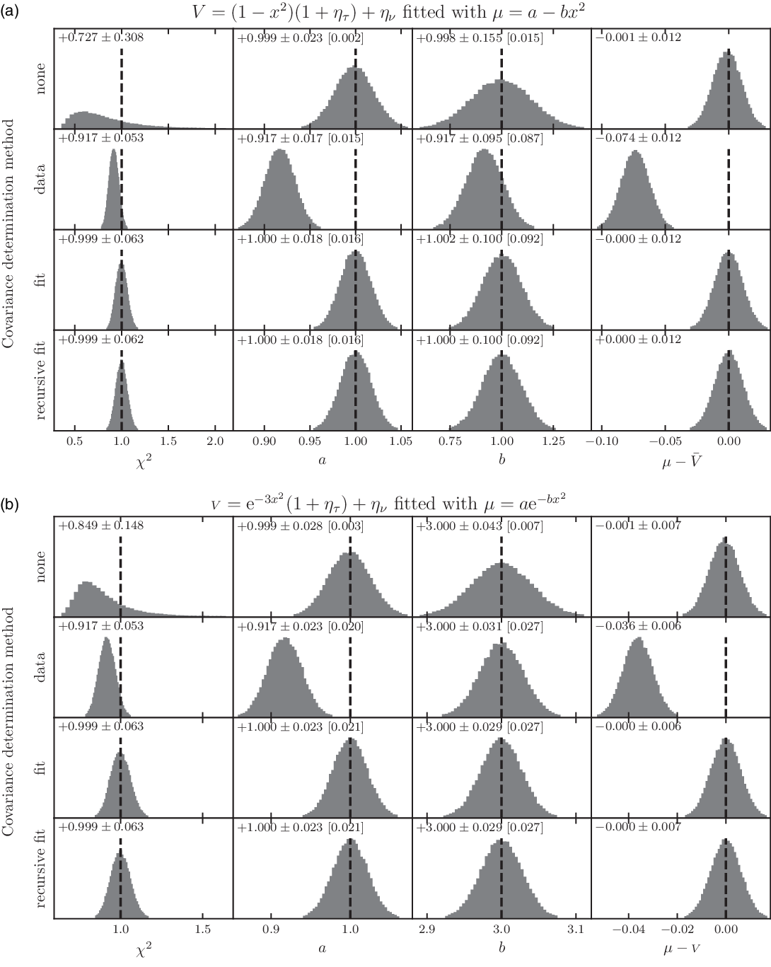
Figure 4(a) sums up the behaviour of the same fit performed a large number of times on different simulated datasets, each following
 ${\scriptstyle V} \approx 1-x^2$
. For each correlation matrix prescription, it displays the dispersion of the reduced chi-squared, the model parameters a and b, and the difference between modelled value and true value. It also reports the uncertainty on model parameters given by the least squares optimisation routine in comparison to the scatter of the distribution of the values. While the model fitting ignoring correlations (method 1) does not show any bias on the parameter estimates, it displays a higher dispersion of model parameters, grossly underestimates the uncertainty on model parameters and has a biased chi-squared. The correlation matrix calculated from data (method 2) is, as expected, strongly biased. Both methods estimating the correlation matrix from modelled data (methods 3 & 4) are equivalent in terms of the absence of bias, dispersion of these quantities, and correct prediction of the uncertainty on model parameters.
${\scriptstyle V} \approx 1-x^2$
. For each correlation matrix prescription, it displays the dispersion of the reduced chi-squared, the model parameters a and b, and the difference between modelled value and true value. It also reports the uncertainty on model parameters given by the least squares optimisation routine in comparison to the scatter of the distribution of the values. While the model fitting ignoring correlations (method 1) does not show any bias on the parameter estimates, it displays a higher dispersion of model parameters, grossly underestimates the uncertainty on model parameters and has a biased chi-squared. The correlation matrix calculated from data (method 2) is, as expected, strongly biased. Both methods estimating the correlation matrix from modelled data (methods 3 & 4) are equivalent in terms of the absence of bias, dispersion of these quantities, and correct prediction of the uncertainty on model parameters.
Given that fitting recursively the covariance matrix does not yield additional benefits for the modelling, I would suggest to use method 3. One would expect this to hold for any smooth enough model, as the update in the covariance matrix is expected to be a small effect. Indeed, I have checked that the result holds for a fully resolved Gaussian disc
 ${\scriptstyle V} \approx \exp -3x^2$
fit by
${\scriptstyle V} \approx \exp -3x^2$
fit by
 $\mu = a\exp -bx^2$
(see Figures 3(b) and 4(b)) a well-resolved binary, with methods 3 & 4 providing unbiased estimates and similar uncertainties. If, for some other application, the model
$\mu = a\exp -bx^2$
(see Figures 3(b) and 4(b)) a well-resolved binary, with methods 3 & 4 providing unbiased estimates and similar uncertainties. If, for some other application, the model
 $\boldsymbol\mu_1$
obtained with method 3 were to differ significantly from the starting guess
$\boldsymbol\mu_1$
obtained with method 3 were to differ significantly from the starting guess
 $\boldsymbol\mu_0$
(method 1), it would certainly make sense to examine whether recursive fitting (method 4) is needed. However, while it converged for the smooth models I tested, I have not proven that it will necessarily do so, in particular for less smooth models that may require it.
$\boldsymbol\mu_0$
(method 1), it would certainly make sense to examine whether recursive fitting (method 4) is needed. However, while it converged for the smooth models I tested, I have not proven that it will necessarily do so, in particular for less smooth models that may require it.
5. Conclusion
The standard covariance propagation, using the measurement values in the calculation, can result in a bias in the model parameters of a least squares fit taking correlations into account. It will occur as soon as the error bars and covariances depend on the measured values, in particular when a normalisation factor, such as the instrumental transfer function of an interferometer, is obtained experimentally. Some bias will even occur without correlations, but the effect is strongest when a large set of correlated data is modelled. This is precisely the case in optical and infrared long-baseline interferometry, where the calibration of spectrally dispersed fringes easily yields
 $10^2$
–
$10^2$
–
 $10^3$
correlated data points.
$10^3$
correlated data points.
While solutions exist that are either numerically expensive or require some care to be implemented (Burr et al. Reference Burr, Kawano, Talou, Pan and Hengartner2011; Becker et al. Reference Becker2012; Nisius Reference Nisius2014), I have shown with a simple example that there is an easy and cheap way to solve the issue. First an uncorrelated fit is performed to estimate the true values corresponding to the data. Secondly, these estimates are used to determine the covariance matrix by error propagation. At last, this covariance matrix is used to perform a least squares model fit.
Alternatively, it is possible to obtain an (almost) unbiased estimate for the model parameters by ignoring correlations altogether, with the cost of a larger imprecision, underestimated uncertainties, and a biased chi-squared. It is, at the moment, the approach taken in the vast majority of published studies in optical interferometry, as data processing pipelines of most instrument do not determine covariances. To my knowledge, Lachaume et al. (Reference Lachaume, Rabus, Jordán, Brahm, Boyajian, von Braun and Berger2019) is the only work where PPP has been explicitly taken care of in optical interferometry.
Acknowledgements
This work has made use of the Smithsonian/NASA Astrophysics Data System (ADS). I thank the anonymous referee for reading the paper carefully and providing constructive remarks, many of which have resulted in changes to the manuscript.
A. Analytical derivation
To shorten summations in the derivation, I introduce
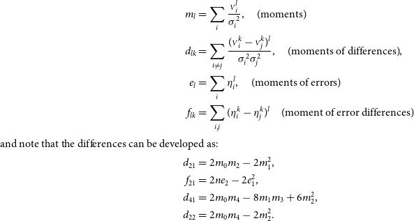 \begin{align*} m_l &= \sum_i \frac{{\scriptstyle V}_i^l}{{\sigma}_i^2}, \quad\text{(moments)}\\ d_{lk} &= \sum_{i \ne j} \frac{({\scriptstyle V}_i^k-{\scriptstyle V}_j^k)^l}{{\sigma}_i^2{\sigma}_j^2}, \quad{({\rm moments\,of\,differences})},\\ e_l &= \sum_i {\eta}_i^l, \quad{({\rm moments\,of\,errors})}\\ f_{lk} &= \sum_{i, j} ({\eta}_i^k - {\eta}_j^k)^l \quad{({\rm moment\,of\,error\,differences})}\\ {\rm {and\,note\,that\,the\,differences\,can\,be\,developed\,as:}}\\d_{21} &= 2m_0m_2 - 2m_1^2,\\ f_{21} &= 2n e_2 - 2e_1^2,\\ d_{41} &= 2m_0m_4 - 8m_1m_3 + 6m_2^2,\\ d_{22} &= 2m_0m_4 - 2m_2^2.\end{align*}
A.1. Equation (16)
I rewrite Equation (14) as:
 \begin{equation*} \{ {{\boldsymbol\Sigma}^{\star}}^{-1} \}_{ij} = \frac{\delta_{ij}}{{\sigma}_i^2} - \frac{\varrho\varsigma_{\tau}^2{{\scriptstyle V}}_i{{\scriptstyle V}}_j} {{\sigma}_i^2{\sigma}_j^2(1 + \varrho\varsigma_{\tau}^2 m_2)}.\end{equation*}
I then proceed from Equation (13):
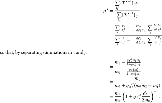 \begin{align*} {\mu}^{\star} &= \frac{\sum\limits_{i,j} \{{{\boldsymbol\Sigma}^{\star}}^{-1}\}_{ij} {{\scriptstyle V}}_i} {\sum\limits_{i,j} \{{{\boldsymbol\Sigma}^{\star}}^{-1}\}_{ij} }\\ &= \frac{\sum\limits_i \frac{{{\scriptstyle V}}_i}{{\sigma}_i^2} - \frac{\varrho\varsigma_{\tau}^2}{1+ \varrho\varsigma_{\tau}^2m_2} \sum\limits_{i,j} \frac{{{\scriptstyle V}}_i^2{{\scriptstyle V}}_j}{{\sigma}_i^2{\sigma}_j^2}} {\sum\limits_i \frac 1{{\sigma}_i^2} - \frac{\varrho\varsigma_{\tau}^2}{1+ \varrho\varsigma_{\tau}^2m_2} \sum\limits_{i,j} \frac{{{\scriptstyle V}}_i{{\scriptstyle V}}_j}{{\sigma}_i^2{\sigma}_j^2}}\\{\rm {so\,that,\,by\,separating\,summations\,in}\,\it{i}\,{\rm and}\,\it{j},} \\&=\frac {m_1-\frac{\varrho\varsigma_{\tau}^2m_1m_2}{1 + \varrho\varsigma_{\tau}^2 m_2}} {m_0-\frac{\varrho\varsigma_{\tau}^2 m_1^2}{1 + \varrho\varsigma_{\tau}^2 m_2}}\\ &= \frac{m_1}{m_0 + \varrho\varsigma_{\tau}^2(m_0m_2 - m_1^2)}\\ &= \frac{m_1}{m_0} \left( 1 + \varrho\varsigma_{\tau}^2\frac{d_{21}}{2m_0} \right)^{-1}.\end{align*}
Equation (16) is obtained by noting that summation over
 $i < j$
is half of that over i, j.
$i < j$
is half of that over i, j.
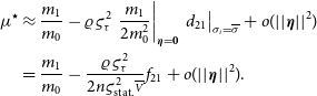
A.2. Equation (17)
Since
 $d_{12}$
is expressed in terms of
$d_{12}$
is expressed in terms of
 $({{\scriptstyle V}}_i - {{\scriptstyle V}}_j)^2 = ({\eta}_i - {\eta}_j)^2$
, the previous equation can be simplified in the second order as:
$({{\scriptstyle V}}_i - {{\scriptstyle V}}_j)^2 = ({\eta}_i - {\eta}_j)^2$
, the previous equation can be simplified in the second order as:
 \begin{align*} {\mu}^{\star} &\approx \frac{m_1}{m_0} - \varrho\varsigma_{\tau}^2 \left. \frac{m_1}{2m_0^2} \right|_{{\boldsymbol\eta} = \boldsymbol 0} \left. d_{21}\right|_{{\sigma}_i = \overline{\sigma}} + o(||{\boldsymbol\eta}||^2)\\ &= \frac{m_1}{m_0} - \frac{\varrho\varsigma_{\tau}^2}{2n{\varsigma_{\text{stat.}}^2}\overline{\scriptstyle V}} f_{21} + o(||{\boldsymbol\eta}||^2).\end{align*}
I now determine the Taylor development for
 \begin{align*} m_l &= \frac{\overline{\scriptstyle V}^{l-2}}{{\varsigma_{\text{stat.}}^2}} \sum_i (1 + {\eta}_i/\overline{\scriptstyle V})^{l-2}\\ m_l &\approx \frac{n\overline{\scriptstyle V}^{l-2}}{{\varsigma_{\text{stat.}}^2}} \left[ 1 + \frac{l-2}{n\overline{\scriptstyle V}}\sum_i {\eta}_i + \frac{(l-2)(l-3)}{2n\overline{\scriptstyle V}^2}\sum_i {\eta}_i^2\right]\\ m_l &\approx \frac{n\overline{\scriptstyle V}^{l-2}}{{\varsigma_{\text{stat.}}^2}}\left[ 1 + \frac{l-2}{n\overline{\scriptstyle V}} e_1 + \frac{(l-2)(l-3)}{2n^2\overline{\scriptstyle V}} e_2 \right],\end{align*}
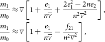
The Taylor developments for
 $m_0$
and
$m_0$
and
 $m_1$
yield
$m_1$
yield
 \begin{align*} \frac{m_1}{m_0} &\approx \overline{\scriptstyle V} \left[ 1 + \frac{e_1}{n\overline{\scriptstyle V}} + \frac{2e_1^2 - 2n e_2}{n^2\overline{\scriptstyle V}^2} \right],\\ \frac{m_1}{m_0} &\approx \overline{\scriptstyle V} \left[ 1 + \frac{e_1}{n\overline{\scriptstyle V}} - \frac{f_{21}}{n^2\overline{\scriptstyle V}^2} \right],\end{align*}
so that
 \begin{equation*} {\mu}^{\star} = \overline{\scriptstyle V} + \frac{e_1}{n} - \frac{1}{\overline{\scriptstyle V}} \left( \frac 1{2n}\frac{\varrho\varsigma_{\tau}^2}{{\varsigma_{\text{stat.}}^2}} + \frac 1{n^2} \right) f_{21}.\end{equation*}
A.3. PPP with photon detection
I model n photon measurements
 $N_i$
of expected value
$N_i$
of expected value
 $\overline{N}$
with noise uncertainty
$\overline{N}$
with noise uncertainty
 $y_i = \sqrt{N_i}$
, showing correlation
$y_i = \sqrt{N_i}$
, showing correlation
 $\varrho$
Footnote h under the assumption of Gaussian errors (
$\varrho$
Footnote h under the assumption of Gaussian errors (
 $\overline N \gg 1$
). The statistical component of the uncertainty is given by
$\overline N \gg 1$
). The statistical component of the uncertainty is given by
 ${\sigma}_i^2 = (1-\varrho)N_i$
. The correlation matrix is
${\sigma}_i^2 = (1-\varrho)N_i$
. The correlation matrix is
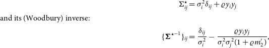 \begin{align*} {\Sigma}^{\star}_{ij} &= {\sigma}_i^2\delta_{ij} + \varrho y_i y_j\\ {{\rm and}\,{\rm its}\,}\,({\rm Woodbury})\,{\rm inverse}:\quad\quad\quad\quad\quad\quad\quad\quad\quad\quad\quad\quad\quad\quad\quad\quad\quad\quad\quad\quad\\\{{{\boldsymbol\Sigma}^{\star}}^{-1}\}_{ij} &= \frac{\delta_{ij}}{{\sigma}_i^2} - \frac{\varrho y_iy_j}{{\sigma}_i^2{\sigma}_j^2(1 + \varrho m^{\prime}_2)},\end{align*}
with the moments
 $m^{\prime}_l$
,
$m^{\prime}_l$
,
 $d^{\prime}_{lk}$
, etc., defined with respect to
$d^{\prime}_{lk}$
, etc., defined with respect to
 $y_i$
, while
$y_i$
, while
 $m_l$
,
$m_l$
,
 $d_{lk}$
, etc., are defined with respect to
$d_{lk}$
, etc., are defined with respect to
 $N_i$
.
$N_i$
.
The least squares estimate for the number of photons is given by:
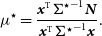 \begin{align*} {\mu}^{\star} &= \frac { {\bf{\it{x}}}^{\text{T}}{{\Sigma}^{\star}}^{-1} \bf{\it{N}} } {{\bf{\it{x}}}^{\text{T}}{{\Sigma}^{\star}}^{-1} \bf{\it{x}} } .\end{align*}
and, by using
 $N_i = y_i^2$
,
$N_i = y_i^2$
,
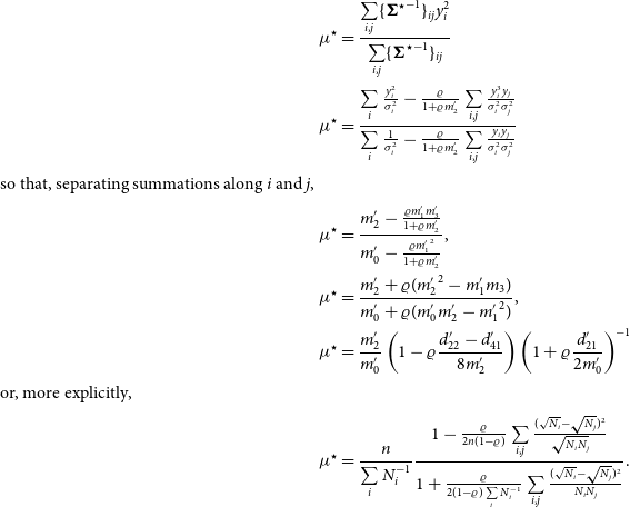 \begin{align*} {\mu}^{\star} &= \frac{\sum\limits_{i,j} \{{{\boldsymbol\Sigma}^{\star}}^{-1}\}_{ij} y_i^2} {\sum\limits_{i,j} \{{{\boldsymbol\Sigma}^{\star}}^{-1}\}_{ij} }\\ {\mu}^{\star} &= \frac{\sum\limits_i \frac{y_i^2}{{\sigma}_i^2} - \frac{\varrho}{1+ \varrho m^{\prime}_2} \sum\limits_{i,j} \frac{y_i^3y_j}{{\sigma}_i^2{\sigma}_j^2}} {\sum\limits_i \frac 1{{\sigma}_i^2} - \frac{\varrho}{1+ \varrho m^{\prime}_2} \sum\limits_{i,j} \frac{y_iy_j}{{\sigma}_i^2{\sigma}_j^2}}\\ {{\rm so\,that,\,separating\,summations\,along}\,\it{i}\,{\rm and}\,\it{j},}\\{\mu}^{\star} &= \frac{m^{\prime}_2 - \frac{\varrho m^{\prime}_1m^{\prime}_3}{1 + \varrho m^{\prime}_2}} {m^{\prime}_0 - \frac{\varrho {m^{\prime}_1}^2}{1 + \varrho m^{\prime}_2}},\\ {\mu}^{\star} &= \frac{m^{\prime}_2 + \varrho({m^{\prime}_2}^2 - m^{\prime}_1m_3)} {m^{\prime}_0 + \varrho(m^{\prime}_0m^{\prime}_2 - {m^{\prime}_1}^2)},\\ {\mu}^{\star} &= \frac{m^{\prime}_2}{m^{\prime}_0} \left(1 - \varrho\frac{d^{\prime}_{22} - d^{\prime}_{41}}{8m^{\prime}_2}\right) \left(1 + \varrho\frac{d^{\prime}_{21}} {2m^{\prime}_0}\right)^{-1}\\ {{\rm or,\,more\,explicitly,}}\quad\quad\quad\quad\quad\quad\quad\quad\quad\quad\quad\\{\mu}^{\star} &= \frac n{\sum\limits_i N_i^{-1}} \frac{ 1 - \frac{\varrho}{2n(1-\varrho)} \sum\limits_{i,j} \frac{(\sqrt{N_i}-\sqrt{N_j})^2}{\sqrt{N_i N_j}} }{ 1 + \frac{\varrho}{2(1-\varrho)\sum\limits_i N_i^{-1}} \sum\limits_{i,j} \frac{(\sqrt{N_i} - \sqrt{N_j})^2}{N_iN_j}} .\end{align*}
In the second order in
 ${\boldsymbol\eta}$
, it can be simplified to
${\boldsymbol\eta}$
, it can be simplified to
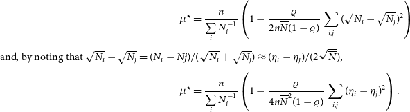 \begin{align*} {\mu}^{\star} &= \frac n{\sum\limits_i N_i^{-1}} \left( 1 - \frac{\varrho}{2n\overline{N}(1-\varrho)} \sum_{i,j} (\sqrt{N_i}-\sqrt{N_j})^2 \right)\\ {\rm {and},\,{\rm by\,noting\,that} \sqrt{N_i} - \sqrt{N_j} = (N_i - Nj) / (\sqrt{N_i} + \sqrt{N_j}) \approx ({\eta}_i - {\eta}_j) / (2\sqrt{\overline{N}}),}\\{\mu}^{\star} &= \frac n{\sum\limits_i N_i^{-1}} \left( 1 - \frac{\varrho}{4n\overline{N}^2(1-\varrho)} \sum_{i,j} ({\eta}_i - {\eta}_j)^2 \right).\end{align*}
The leading factor can be approximated in the second order using the Taylor series:
 \begin{align*} \sum_i N_i^{-1} \approx \frac{n}{\overline{N}} - \frac{e_1}{\overline{N}^2} + \frac{e_2}{\overline{N}^3}\\ {\rm so\,that}\quad\quad\quad\quad\quad\quad\quad\quad\quad\quad\quad\quad\quad\quad\quad\quad\quad\quad\quad\frac{n}{\sum\limits_i N_i^{-1}} \approx \overline{N} + \frac{e_1}{n} + \frac{e_1^2-ne_2}{n^2\overline{N}},\\ \frac{n}{\sum\limits_i N_i^{-1}} \approx \overline{N} + \frac{e_1}{n} - \frac{f_{21}}{2n^2\overline{N}}.\end{align*}
Finally,
 \begin{align*} {\mu}^{\star} &\approx \overline{N} + \frac{\sum\limits_i {\eta}_i}{n} - \left(1 + \frac{n\varrho}{2(1-\varrho)} \right) \frac{\sum\limits_{i,j} ({\eta}_i - {\eta}_j) ^2}{2Nn^2}.\end{align*}
With
 $<{({\eta}_i-{\eta}_j)^2}> = 2(1-\varrho)\overline{N}$
and
$<{({\eta}_i-{\eta}_j)^2}> = 2(1-\varrho)\overline{N}$
and
 $<{{\eta}_i}> = 0$
, the bias of the best-fit estimate for the average number of photons is
$<{{\eta}_i}> = 0$
, the bias of the best-fit estimate for the average number of photons is
 \begin{align*} <{{\mu}^{\star}}> &\approx \overline{N} - \left(1 - \frac 1n\right) \left( (1-\varrho) + \frac{n\varrho}{2}\right)\end{align*}
or, with the relative statistical and systematic uncertainties
 ${\varsigma_{\text{stat.}}^2} = (1-\varrho)/\overline{N}$ and ${\varsigma_{\text{sys.}}^2} = \varrho/\overline{N}$
,
${\varsigma_{\text{stat.}}^2} = (1-\varrho)/\overline{N}$ and ${\varsigma_{\text{sys.}}^2} = \varrho/\overline{N}$
,
 \begin{align*} <{{\mu}^{\star}}> &\approx \overline{N} \left[ 1 - \left(1 - \frac 1n\right) \left({\varsigma_{\text{stat.}}^2} + \frac n2 {\varsigma_{\text{sys.}}^2}\right)\right].\end{align*}
The bias from PPP is exactly half of that determined for normalisation errors in the main part of the paper. It shows that the effect does not necessarily arise from a normalisation.


 Open access