


1. Introduction
We consider a class of inhomogeneous Erdős–Rényi random graphs on n vertices. Our vertex set V is denoted by
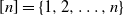 $[n]=\{1, 2, \ldots, n\}$
and on each vertex we assign independent weights (or ‘fitness’ variables)
$[n]=\{1, 2, \ldots, n\}$
and on each vertex we assign independent weights (or ‘fitness’ variables)
 $(W_i)_{i\in [n]}$
distributed according to a common distribution
$(W_i)_{i\in [n]}$
distributed according to a common distribution
 $F_W(\! \cdot \!)$
with
$F_W(\! \cdot \!)$
with
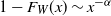 $1-F_W(x)\sim x^{-\alpha}$
for some
$1-F_W(x)\sim x^{-\alpha}$
for some
 $\alpha\in (0,1)$
. Therefore, the weights have infinite mean. Conditioned on the weights, an edge between two distinct vertices i and j is drawn independently with probability
$\alpha\in (0,1)$
. Therefore, the weights have infinite mean. Conditioned on the weights, an edge between two distinct vertices i and j is drawn independently with probability
 \begin{equation} p_{ij}= 1-\exp\! (\!-\!\varepsilon W_i W_j),\end{equation}
where
 $\varepsilon$
is a parameter tuning the overall density of edges in the graph and playing a crucial rule in the analysis of the model. This inhomogeneous random graph model with infinite-mean weights has recently been proposed in [Reference Garuccio, Lalli and Garlaschelli19] in the statistical physics literature, where it was studied as a scale-invariant random graph under hierarchical coarse-graining of vertices. In particular, the model follows from the fundamental requirement that both the connection probability
$\varepsilon$
is a parameter tuning the overall density of edges in the graph and playing a crucial rule in the analysis of the model. This inhomogeneous random graph model with infinite-mean weights has recently been proposed in [Reference Garuccio, Lalli and Garlaschelli19] in the statistical physics literature, where it was studied as a scale-invariant random graph under hierarchical coarse-graining of vertices. In particular, the model follows from the fundamental requirement that both the connection probability
 $p_{ij}$
and the fitness distribution
$p_{ij}$
and the fitness distribution
 $F_W(x)$
retain the same mathematical form when applied to the ‘renormalized’ graph obtained by agglomerating vertices into equally sized ‘supervertices’, where the fitness of each supervertex is defined as the sum of the fitnesses of the constituent vertices [Reference Garuccio, Lalli and Garlaschelli19]. This agglomeration process provides a renormalization scheme for the graph [Reference Gabrielli, Garlaschelli, Patil and Serrano16] that, by admitting any homogeneous partition of vertices, does not require the notion of vertex coordinates in some underlying metric space, unlike other models based on the idea of geometric renormalization where ‘closer’ vertices are merged [Reference Boguna, Bonamassa, De Domenico, Havlin, Krioukov and Serrano7, Reference Garca-Pérez, Boguñá and Serrano17]. We summarize the main ideas behind the original model later in this paper.
$F_W(x)$
retain the same mathematical form when applied to the ‘renormalized’ graph obtained by agglomerating vertices into equally sized ‘supervertices’, where the fitness of each supervertex is defined as the sum of the fitnesses of the constituent vertices [Reference Garuccio, Lalli and Garlaschelli19]. This agglomeration process provides a renormalization scheme for the graph [Reference Gabrielli, Garlaschelli, Patil and Serrano16] that, by admitting any homogeneous partition of vertices, does not require the notion of vertex coordinates in some underlying metric space, unlike other models based on the idea of geometric renormalization where ‘closer’ vertices are merged [Reference Boguna, Bonamassa, De Domenico, Havlin, Krioukov and Serrano7, Reference Garca-Pérez, Boguñá and Serrano17]. We summarize the main ideas behind the original model later in this paper.
More generally, (1.1) represents a special example of connection probability between vertices i and j defined as
 $\kappa_n(W_i,W_j)$
, where
$\kappa_n(W_i,W_j)$
, where
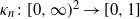 $\kappa_n\colon [0,\infty)^2\to [0,1]$
is a well-behaved function and the weights are drawn independently from a certain distribution. In the physics literature, these are called ‘fitness’ or ‘hidden variable’ network models [Reference Boguná and Pastor-Satorras8, Reference Caldarelli, Capocci, De Los Rios and Munoz10, Reference Garlaschelli, Capocci and Caldarelli18]. In the mathematical literature, a well-known example is the generalized random graph model [Reference Chung and Lu11, Reference van der Hofstad31]. In most cases considered in the literature so far, due to the integrability conditions on
$\kappa_n\colon [0,\infty)^2\to [0,1]$
is a well-behaved function and the weights are drawn independently from a certain distribution. In the physics literature, these are called ‘fitness’ or ‘hidden variable’ network models [Reference Boguná and Pastor-Satorras8, Reference Caldarelli, Capocci, De Los Rios and Munoz10, Reference Garlaschelli, Capocci and Caldarelli18]. In the mathematical literature, a well-known example is the generalized random graph model [Reference Chung and Lu11, Reference van der Hofstad31]. In most cases considered in the literature so far, due to the integrability conditions on
 $\kappa_n$
and moment properties of
$\kappa_n$
and moment properties of
 $F_W$
, these models have a locally tree-like structure. We refer to [Reference van der Hofstad32, Chapter 6] for the properties of the degree distribution and to [Reference Bollobás, Janson and Riordan9, Reference van der Hofstad33] for further geometric structures. Models with exactly the same connection probability as in (1.1), but with finite-mean weights, have previously been considered [Reference Bhamidi, van der Hofstad and Sen3, Reference Bhamidi, van der Hofstad and van Leeuwaarden4, Reference Norros and Reittu24, Reference Rodgers, Austin, Kahng and Kim27, Reference van der Hofstad31]. In this article we are instead interested in the non-standard case of infinite-mean weights, corresponding to the choice
$F_W$
, these models have a locally tree-like structure. We refer to [Reference van der Hofstad32, Chapter 6] for the properties of the degree distribution and to [Reference Bollobás, Janson and Riordan9, Reference van der Hofstad33] for further geometric structures. Models with exactly the same connection probability as in (1.1), but with finite-mean weights, have previously been considered [Reference Bhamidi, van der Hofstad and Sen3, Reference Bhamidi, van der Hofstad and van Leeuwaarden4, Reference Norros and Reittu24, Reference Rodgers, Austin, Kahng and Kim27, Reference van der Hofstad31]. In this article we are instead interested in the non-standard case of infinite-mean weights, corresponding to the choice
 $\alpha\in (0,1)$
as mentioned above. The combination of the specific form of the connection probability (1.1) and these heavy-tailed weights makes the model interesting. We believe that certain mathematical features of an ultra-small world network, where the degrees exhibit infinite variance, can be captured by this model. In this case, due to the absence of a finite mean, the typical distances may be much slower than the doubly logarithmic behavior (in relation to the graph’s size) observed in ultra-small networks (refer to [Reference van der Hofstad and Komjáthy36] for further discussion on this).
$\alpha\in (0,1)$
as mentioned above. The combination of the specific form of the connection probability (1.1) and these heavy-tailed weights makes the model interesting. We believe that certain mathematical features of an ultra-small world network, where the degrees exhibit infinite variance, can be captured by this model. In this case, due to the absence of a finite mean, the typical distances may be much slower than the doubly logarithmic behavior (in relation to the graph’s size) observed in ultra-small networks (refer to [Reference van der Hofstad and Komjáthy36] for further discussion on this).
Another model where a connection probability similar to (1.1) occurs, but with an additional notion of embedding geometry, is the scale-free percolation model on
 $\mathbb{Z}^d$
. The vertex set in this graph is no longer a finite set of points, and the connection probabilities also depend on the spatial positions of the vertices. Here we also start with independent weights
$\mathbb{Z}^d$
. The vertex set in this graph is no longer a finite set of points, and the connection probabilities also depend on the spatial positions of the vertices. Here we also start with independent weights
 $(W_x)_{x\in \mathbb{Z}^d}$
distributed according to
$(W_x)_{x\in \mathbb{Z}^d}$
distributed according to
 $F_W(\! \cdot \!)$
, where
$F_W(\! \cdot \!)$
, where
 $F_W$
has a power law index of
$F_W$
has a power law index of
 $\beta\in (0, \infty)$
; conditioned on the weights, vertices x and y are connected independently with probability
$\beta\in (0, \infty)$
; conditioned on the weights, vertices x and y are connected independently with probability
 \begin{align*}\tilde p_{xy}= 1-\exp\bigg({-}\frac{\lambda W_x W_y}{\|x-y\|^s}\bigg),\end{align*}
where s and
 $\lambda$
are some positive parameters. The model was introduced in [Reference Deijfen, van der Hofstad and Hooghiemstra13], where it was shown that the degree of distribution has a power-law exponent of parameter
$\lambda$
are some positive parameters. The model was introduced in [Reference Deijfen, van der Hofstad and Hooghiemstra13], where it was shown that the degree of distribution has a power-law exponent of parameter
 $-\tau=-s\beta/d$
. The asymptotics of the maximum degree was derived recently in [Reference Bhattacharjee and Schulte5] and further properties of the chemical distances were studied in [Reference Deprez, Hazra and Wüthrich14, Reference Heydenreich, Hulshof and Jorritsma21, Reference van der Hofstad and Komjathy35]. In some cases the degree can be infinite too. The mixing properties of the scale-free percolation on a torus of side length n was studied in [Reference Cipriani and Salvi12]. In our model, the distance term
$-\tau=-s\beta/d$
. The asymptotics of the maximum degree was derived recently in [Reference Bhattacharjee and Schulte5] and further properties of the chemical distances were studied in [Reference Deprez, Hazra and Wüthrich14, Reference Heydenreich, Hulshof and Jorritsma21, Reference van der Hofstad and Komjathy35]. In some cases the degree can be infinite too. The mixing properties of the scale-free percolation on a torus of side length n was studied in [Reference Cipriani and Salvi12]. In our model, the distance term
 $\|x-y\|^{-s}$
is not present and hence on one hand the form becomes easier, but on the other hand many useful integrability properties are lost due to the fact that interactions do not decay with distance.
$\|x-y\|^{-s}$
is not present and hence on one hand the form becomes easier, but on the other hand many useful integrability properties are lost due to the fact that interactions do not decay with distance.
In this paper we show some important properties of our model. In particular, we show that the average degree grows like
 $\log n$
if we choose the specific scaling
$\log n$
if we choose the specific scaling
 $\varepsilon= n^{-{1}/{\alpha}}$
. In this case, the cumulative degree distribution behaves roughly like a power law with exponent
$\varepsilon= n^{-{1}/{\alpha}}$
. In this case, the cumulative degree distribution behaves roughly like a power law with exponent
 $-1$
. In the literature for random graphs with degree sequences having infinite mean, this falls in the critical case of exponent
$-1$
. In the literature for random graphs with degree sequences having infinite mean, this falls in the critical case of exponent
 $\tau=1$
. The configuration model with given degree sequence
$\tau=1$
. The configuration model with given degree sequence
 $(D_i)_{i\in [n]}$
, independently and identically distributed with law D having a power-law exponent
$(D_i)_{i\in [n]}$
, independently and identically distributed with law D having a power-law exponent
 $\tau\in (0,1)$
, was studied in [Reference van den Esker, van der Hofstad, Hooghiemstra and Znamenski30]. It was shown that the typical distance between two randomly chosen points is either 2 or 3. It was also shown that for
$\tau\in (0,1)$
, was studied in [Reference van den Esker, van der Hofstad, Hooghiemstra and Znamenski30]. It was shown that the typical distance between two randomly chosen points is either 2 or 3. It was also shown that for
 $\tau=1$
similar ultra-small-world behavior is true. Instead of the configuration model, we study the properties of the degree distribution for the model, which also naturally gives rise to degree distributions with power-law exponent
$\tau=1$
similar ultra-small-world behavior is true. Instead of the configuration model, we study the properties of the degree distribution for the model, which also naturally gives rise to degree distributions with power-law exponent
 $-1$
. Additionally, we investigate certain dependencies between the degrees of different vertices, the asymptotic density of wedges and triangles, and some first observations on the subtle connectivity properties of the random graph.
$-1$
. Additionally, we investigate certain dependencies between the degrees of different vertices, the asymptotic density of wedges and triangles, and some first observations on the subtle connectivity properties of the random graph.
The rest of the paper is organized as follows: in Section 2 we state our main results, in Section 3 we discuss the connection to the original model [Reference Garuccio, Lalli and Garlaschelli19], and finally in Sections 4, 5, and 6 we prove our results.
2. Model and main results
The formal definition of the model considered here reads as follows. Let the vertex set be given by
 $[n]= \{1,2, \ldots, n\}$
and let
$[n]= \{1,2, \ldots, n\}$
and let
 $\varepsilon=\varepsilon_n\, {\gt} \,0$
be a parameter that depends on n. For notational simplicity, we will drop the subscript n from
$\varepsilon=\varepsilon_n\, {\gt} \,0$
be a parameter that depends on n. For notational simplicity, we will drop the subscript n from
 $\varepsilon_n$
throughout the paper, except where the context needs it. The random graph with law
$\varepsilon_n$
throughout the paper, except where the context needs it. The random graph with law
 $\mathbb{P}$
is constructed in the following way:
$\mathbb{P}$
is constructed in the following way:
-
(i) Sample n independent weights
 $(W_i)$
, under
$\mathbb{P}$
, according to a Pareto distribution with parameter
$\alpha\in (0, 1)$
, i.e. (2.1)
\begin{equation} 1- F_W(w)=\mathbb{P}(W_i\, {\gt} \, w)=\begin{cases} w^{-\alpha}, & w\, {\gt} \,1, \\ 1, & 0{\, \lt} \, w\le 1.\end{cases}. \end{equation}
$(W_i)$
, under
$\mathbb{P}$
, according to a Pareto distribution with parameter
$\alpha\in (0, 1)$
, i.e. (2.1)
\begin{equation} 1- F_W(w)=\mathbb{P}(W_i\, {\gt} \, w)=\begin{cases} w^{-\alpha}, & w\, {\gt} \,1, \\ 1, & 0{\, \lt} \, w\le 1.\end{cases}. \end{equation}
-
(ii) For all
$n\ge 1$
, given the weights
$(W_i)_{i\in [n]}$
, construct the random graph
$G_n$
by joining edges independently with probability given by (1.1). That is, (2.2)where the event
\begin{equation} p_{ij}\;:\!=\;\mathbb{P}( i \leftrightarrow j\mid W_i, W_j)= 1-\exp \! (\!-\! \varepsilon W_i W_j), \end{equation}
$\{i\leftrightarrow j\}$
means that vertices i and j are connected by an edge in the graph.


We will denote the above random graph by
 $\mathbf{G}_n(\alpha,\varepsilon)$
as it depends on the parameters
$\mathbf{G}_n(\alpha,\varepsilon)$
as it depends on the parameters
 $\alpha$
and
$\alpha$
and
 $\varepsilon$
. Self-loops and multi-edges are not allowed, and hence the final graph is given by a simple graph on n vertices. Note that in choosing the distribution of the weights in (2.1) we could alternatively have started with a regularly varying random variable with power-law exponent
$\varepsilon$
. Self-loops and multi-edges are not allowed, and hence the final graph is given by a simple graph on n vertices. Note that in choosing the distribution of the weights in (2.1) we could alternatively have started with a regularly varying random variable with power-law exponent
 $-\alpha$
, i.e.
$-\alpha$
, i.e.
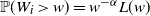 $\mathbb{P}(W_i\, {\gt} \,w)= w^{-\alpha} L(w)$
where
$\mathbb{P}(W_i\, {\gt} \,w)= w^{-\alpha} L(w)$
where
 $L(\! \cdot \!)$
is a slowly varying function, i.e., for any
$L(\! \cdot \!)$
is a slowly varying function, i.e., for any
 $t\, {\gt} \,0$
,
$t\, {\gt} \,0$
,
 \begin{align*}\lim_{w\to\infty}\frac{L(wt)}{L(w)}=1.\end{align*}
It is our belief that most of the results stated in this article will go through in the presence of a slowly varying function, even if the analysis is more involved. In particular, as we explain in Section 3, in the approach of [Reference Garuccio, Lalli and Garlaschelli19] the weights are drawn from a one-sided
 $\alpha$
-stable distribution with scale parameter
$\alpha$
-stable distribution with scale parameter
 $\gamma$
, and not from a Pareto (the
$\gamma$
, and not from a Pareto (the
 $\alpha$
-stable following from the requirement of invariance of the fitness distribution under graph renormalization). We expect that the computations will go through if we assume
$\alpha$
-stable following from the requirement of invariance of the fitness distribution under graph renormalization). We expect that the computations will go through if we assume
 $\mathbb{P}(W_i\, {\gt} \,w)\sim w^{-\alpha}$
as
$\mathbb{P}(W_i\, {\gt} \,w)\sim w^{-\alpha}$
as
 $w\to\infty$
, which is the case for
$w\to\infty$
, which is the case for
 $\alpha$
-stable distributions. In this work, however, we refrain from going into this technical side.
$\alpha$
-stable distributions. In this work, however, we refrain from going into this technical side.
In terms of notation, convergence in distribution and convergence in probability will be denoted respectively by
 $\overset{\textrm{d}}\longrightarrow$
and
$\overset{\textrm{d}}\longrightarrow$
and
 $\overset{P}\longrightarrow$
.
$\overset{P}\longrightarrow$
.
 $\mathbb{E}[\! \cdot \!]$
is the expectation with respect to
$\mathbb{E}[\! \cdot \!]$
is the expectation with respect to
 $\mathbb{P}$
, and the conditional expectation with respect to the weight W of a typical vertex is denoted by
$\mathbb{P}$
, and the conditional expectation with respect to the weight W of a typical vertex is denoted by
 $\mathbb{E}_W[\! \cdot \!] = \mathbb{E}[\cdot \mid W]$
. We write
$\mathbb{E}_W[\! \cdot \!] = \mathbb{E}[\cdot \mid W]$
. We write
 $X \mid W$
to denote the distribution of the random variable X conditioned on the variable W. Let
$X \mid W$
to denote the distribution of the random variable X conditioned on the variable W. Let
 $(a_{ij})_{1\leq i, j\leq n}$
be the indicator variables
$(a_{ij})_{1\leq i, j\leq n}$
be the indicator variables
 $(\mathbf {1}_{i\leftrightarrow j})_{1\leq i, j\leq n}$
. As standard, as
$(\mathbf {1}_{i\leftrightarrow j})_{1\leq i, j\leq n}$
. As standard, as
 $n\to \infty$
we will write
$n\to \infty$
we will write
 $f(n)\sim g(n)$
if
$f(n)\sim g(n)$
if
 $f(n)/g(n)\to 1$
,
$f(n)/g(n)\to 1$
,
 $f(n)=o\!\left(g(n)\right)$
if
$f(n)=o\!\left(g(n)\right)$
if
 $f(n)/g(n)\to 0$
, and
$f(n)/g(n)\to 0$
, and
 $f(n)=O\!\left(g(n)\right)$
if
$f(n)=O\!\left(g(n)\right)$
if
 $f(n)/g(n)\leq C$
for some
$f(n)/g(n)\leq C$
for some
 $C\, {\gt} \,0$
, for n large enough. Lastly,
$C\, {\gt} \,0$
, for n large enough. Lastly,
 $f(n)\asymp g(n)$
denotes that there exist positive constants
$f(n)\asymp g(n)$
denotes that there exist positive constants
 $c_1$
and
$c_1$
and
 $C_2$
such that
$C_2$
such that
 \begin{align*}c_1 \le \liminf_{n\to\infty}\frac{f(n)}{g(n)} \le \limsup_{n\to\infty}\frac{f(n)}{g(n)} \le C_2.\end{align*}
Finally, we use
 $A\vee B$
to represent
$A\vee B$
to represent
 $\max\{A, B\}$
, the maximum of two numbers A and B.
$\max\{A, B\}$
, the maximum of two numbers A and B.
2.1. Degrees
Our first theorem characterizes the behavior of a typical degree and of the joint distribution of the degrees. Consider the degree of vertex
 $i\in [n]$
, defined as
$i\in [n]$
, defined as
 $D_n(i) = \sum_{j\neq i} a_{ij}$
, where
$D_n(i) = \sum_{j\neq i} a_{ij}$
, where
 $a_{ij}$
denotes the entries of the adjacency matrix of the graph, i.e.
$a_{ij}$
denotes the entries of the adjacency matrix of the graph, i.e.
 \begin{align*}a_{ij}= \begin{cases} 1 & \text{if $i\leftrightarrow j$}, \\ 0 & \text{otherwise}.\end{cases}\end{align*}
Theorem 2.1 (Scaling and asymptotics of the degrees.) Consider the graph
 $\mathbf{G}_n(\alpha, \varepsilon)$
and let
$\mathbf{G}_n(\alpha, \varepsilon)$
and let
 $D_n(i)$
be the degree of the vertex
$D_n(i)$
be the degree of the vertex
 $i\in [n]$
.
$i\in [n]$
.
-
(i) Expected degree: The expected degree of a vertex i scales as
as
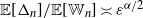
\begin{align*}\mathbf{E}[D_n(i)] \sim - (n-1) \Gamma(1-\alpha) \varepsilon^{\alpha} \log{\varepsilon^{\alpha}}\end{align*}
$\varepsilon\downarrow 0$
. In particular, if
$\varepsilon= n^{-1/\alpha}$
then we have (2.3)
\begin{equation} \mathbb{E}[D_n(i)] \sim \Gamma(1-\alpha) \log n \quad \text{as}\ n\to \infty. \end{equation}
-
(ii) Asymptotic degree distribution: Let
$\varepsilon = n^{-{1}/{\alpha}}$
. Then, for all
$i\in [n]$
,
$D_n(i) \overset{\textrm{d}}\longrightarrow D_{\infty}$
as
$n\to\infty$
, where
$D_\infty$
is a mixed Poisson random variable with parameter
$\Lambda = \Gamma(1-\alpha) W^{\alpha}$
, where W has distribution (2.1). Additionally, we have (2.4)
\begin{equation} \mathbb{P}(D_\infty\, {\gt} \, x) \sim \Gamma(1-\alpha) x^{-1} \quad \text{as $x\to\infty$}. \end{equation}
-
(iii) Asymptotic joint degree behavior: Let
$D_\infty(i)$
and
$D_\infty(\, j)$
be the asymptotic degree distributions of two arbitrary distinct vertices
$i,j\in\mathbb{N}$
. Then (2.5)and for s, t sufficiently close to 1 we have
\begin{equation} \mathbb{E}\big[t^{D_\infty(i)}s^{D_\infty(\, j)}\big] \neq \mathbb{E}\big[t^{D_\infty(i)}\big]\mathbb{E}\big[s^{D_\infty(\, j)}\big] \quad \text{for fixed}\ t, s\in (0,1), \end{equation}
(2.6)for some constant
\begin{align} & \big{|}\mathbb{E}\big[t^{D_\infty(i)}s^{D_\infty(\, j)}\big] - \mathbb{E}\big[t^{D_\infty(i)}\big]\mathbb{E}\big[s^{D_\infty(\, j)}\big]\big{|} \nonumber \\ & \qquad \leq \textrm{O}\bigg((1-s)(1-t)\log\bigg(\bigg(1+\frac{1}{\Gamma(1-\alpha)(1-s)}\bigg) \bigg(1+\frac{1}{\Gamma(1-\alpha)(1-t)}\bigg)\bigg)\bigg) \nonumber \\ & \qquad\quad + C((1-t)+(1-s)) \end{align}
$C\in (0,\infty)$
.


We prove Theorem 2.1 in Section 4. The first part of the result shows that, in the chosen regime, the average degree of the graph diverges logarithmically. This indeed rules out any kind of local weak limit of the graph. We also see in the second part that, asymptotically, degrees have cumulative power-law exponent
 $-1$
, for any
$-1$
, for any
 $\alpha\in(0,1)$
. This rigorously proves a result that was observed with different analytical and numerical arguments in the original paper [Reference Garuccio, Lalli and Garlaschelli19], as we further discuss in Section 3. It is expected that when
$\alpha\in(0,1)$
. This rigorously proves a result that was observed with different analytical and numerical arguments in the original paper [Reference Garuccio, Lalli and Garlaschelli19], as we further discuss in Section 3. It is expected that when
 $\varepsilon=n^{-1/\alpha}$
, we should have
$\varepsilon=n^{-1/\alpha}$
, we should have
 $\mathbb{P}( D_n(i)\, {\gt} \,x)\asymp x^{-1}$
as
$\mathbb{P}( D_n(i)\, {\gt} \,x)\asymp x^{-1}$
as
 $x\to \infty$
.
$x\to \infty$
.
The third part of the result deserves further comment. Indeed, (2.5) shows that
 $D_\infty(i)$
and
$D_\infty(i)$
and
 $D_\infty(\, j)$
are not independent. In the generalized random graph model, this is a surprising phenomenon. If we consider a generalized random graph with weights as described in (2.1) and
$D_\infty(\, j)$
are not independent. In the generalized random graph model, this is a surprising phenomenon. If we consider a generalized random graph with weights as described in (2.1) and
 \begin{align*}\widetilde p_{ij}= \frac{ W_i W_j}{n^{1/\alpha}+ W_i W_j},\end{align*}
then it follows from [Reference van der Hofstad32, Theorem 6.14] that the asymptotic degree distribution has the same behavior as our model and the asymptotic degree distributions are independent. Although there is no independence as (2.5) shows, we still believe that
 \begin{equation} \big{|}\mathbb{P}(D_\infty(i) \, {\gt} \, x, D_\infty(\, j) \, {\gt} \, x)-\mathbb{P}( D_\infty(i)\, {\gt} \,x) \mathbb{P}( D_{\infty}(\, j)\, {\gt} \,x)\big{|} = \textrm{o}(\mathbb{P}( D_\infty(i)\, {\gt} \,x) \mathbb{P}( D_{\infty}(\, j)\, {\gt} \,x))\end{equation}
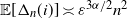
holds, and hence the limiting vector will be asymptotically tail independent. Although not provided with a rigorous proof yet, this conjecture is supported by numerical simulations (see Fig. 1). Such a property of limiting degree was observed and proved using a multivariate version of Karamata’s Tauberian theorem for preferential attachment models, see [Reference Resnick and Samorodnitsky26]. In our case, (2.7) would be valid, given an explicit characterization of the complete joint distribution of the asymptotic degrees. Currently, we have not been able to verify the conditions outlined in [Reference Resnick and Samorodnitsky26] for the application of their general multivariate Tauberian theorem. We hope to address this question in the future.
Asymptotic tail independence between degrees. Scatterplot of the degrees of the vertices with labels 1 and 2 (assigned randomly but fixed for every realization in the ensemble). Each point in the plot corresponds to one of 2000 realizations of a network of
 $N=2000$
vertices, each generated as described at the beginning of Section 2 (see (2.1) and (2.2)).
$N=2000$
vertices, each generated as described at the beginning of Section 2 (see (2.1) and (2.2)).

2.2. Wedges, triangles, and clustering
Our second result concerns the number of wedges and triangles associated with a typical vertex
 $i\in[n]$
, defined respectively as
$i\in[n]$
, defined respectively as
 \begin{equation*} \mathbb{W}_n(i) \;:\!=\; \frac{1}{2} \sum_{j\neq i} \sum_{k\neq i,j} a_{ij} a_{ik}, \qquad \Delta_n(i) = \frac{1}{6} \sum_{j\neq i} \sum_{k\neq i,j} a_{ij} a_{ik} a_{jk}.\end{equation*}
Theorem 2.2. (Triangles and wedges of typical vertices.) Consider the graph
 $\mathbf{G}_n(\alpha, \varepsilon)$
and let
$\mathbf{G}_n(\alpha, \varepsilon)$
and let
 $\mathbb{W}_n(i)$
and
$\mathbb{W}_n(i)$
and
 $\Delta_n(i)$
be the numbers of wedges and triangles at vertex
$\Delta_n(i)$
be the numbers of wedges and triangles at vertex
 $i\in [n]$
. Then:
$i\in [n]$
. Then:
-
(i) Average number of wedges:
$\mathbb{E}[\mathbb{W}_n(i)] \asymp \varepsilon^{\alpha} n^2$
as
$\varepsilon\downarrow 0$
. In particular, when
$\varepsilon = n^{-1/\alpha}$
,
$\mathbb{E}[\mathbb{W}_n(i)] \asymp n$
. -
(ii) Asymptotic distribution of wedges: Let
$\varepsilon = n^{-1/\alpha}$
. Then
$\mathbb{W}_n(i) \overset{\textrm{d}}{\longrightarrow} \mathbb{W}_{\infty}(i)$
, where
$\mathbb{W}_{\infty}(i) = D_{\infty}(i)(D_{\infty}(i)-1)$
with
$D_{\infty}(i)$
as in Theorem 2.1. Also,
\begin{align*}\mathbb{P}(\mathbb{W}_{\infty}(i)\, {\gt} \, x ) \sim \Gamma(1-\alpha)x^{-1/2} \quad \text{as}\ x\to\infty.\end{align*}
-
(iii) Average number of triangles: Let
$i\in [n]$
. The average number of triangles grows as
$\mathbb{E}[\Delta_n(i)] \asymp \varepsilon^{{3\alpha}/{2}}n^2$
as
$\varepsilon\downarrow 0$
. In particular, when
$\varepsilon=n^{-1/\alpha}$
we have
$\mathbb{E}[\Delta_n(i)] \asymp \sqrt{n}$
as
$n\to \infty$
. -
(iv) Concentration for the number of triangles: Let
$\varepsilon= n^{-1/\alpha}$
and
$\Delta_n=\sum_{i\in [n]} \Delta_n(i)$
be the total number of triangles. Then
\begin{align*} \frac{\Delta_n}{\mathbb{E}[\Delta_n]} \overset{\mathbb{P}}\longrightarrow 1, \qquad \frac{\Delta_n(i)}{\mathbb{E}[\Delta_n(i)]} \overset{\mathbb{P}}\longrightarrow 1. \end{align*}


Remark 2.1. (Global and local clustering.) Let
 $\mathbb{W}_n=\sum_{i\in [n]}\mathbb{W}_n(i)$
be the total number of wedges. We see from Theorem 2.2 that
$\mathbb{W}_n=\sum_{i\in [n]}\mathbb{W}_n(i)$
be the total number of wedges. We see from Theorem 2.2 that
 $\mathbb{E}[\Delta_n]/\mathbb{E}[\mathbb{W}_n] \asymp \varepsilon^{\alpha/2}$
as
$\mathbb{E}[\Delta_n]/\mathbb{E}[\mathbb{W}_n] \asymp \varepsilon^{\alpha/2}$
as
 $\varepsilon \to 0$
. This shows in a quantitative form that the graph is not highly clustered from the point of view of the global count of triangles. In particular, in the scale of
$\varepsilon \to 0$
. This shows in a quantitative form that the graph is not highly clustered from the point of view of the global count of triangles. In particular, in the scale of
 $\varepsilon = n^{-1/\alpha}$
, the above ratio goes to zero like
$\varepsilon = n^{-1/\alpha}$
, the above ratio goes to zero like
 $n^{-1/2}$
. However, this does not mean that the graph is not highly clustered from the point of view of the local count of triangles around individual vertices. Indeed, simulations in [Reference Garuccio, Lalli and Garlaschelli19] of the average local clustering coefficient suggest that the graph is locally clustered (see also Section 3). A dissimilarity in the behavior of local and global clustering coefficients has also been observed in different inhomogeneous random graph models; see, for example, [Reference Michielan, Litvak and Stegehuis23, Reference van der Hofstad, Janssen, van Leeuwaarden and Stegehuis34, Reference van der Hofstad, Van der Hoorn, Litvak and Stegehuis37]. We do not consider the local clustering here.
$n^{-1/2}$
. However, this does not mean that the graph is not highly clustered from the point of view of the local count of triangles around individual vertices. Indeed, simulations in [Reference Garuccio, Lalli and Garlaschelli19] of the average local clustering coefficient suggest that the graph is locally clustered (see also Section 3). A dissimilarity in the behavior of local and global clustering coefficients has also been observed in different inhomogeneous random graph models; see, for example, [Reference Michielan, Litvak and Stegehuis23, Reference van der Hofstad, Janssen, van Leeuwaarden and Stegehuis34, Reference van der Hofstad, Van der Hoorn, Litvak and Stegehuis37]. We do not consider the local clustering here.
2.3. Connectedness: Some first observations
Connectivity properties of inhomogeneous random graphs were studied in the sparse setting in [Reference Bollobás, Janson and Riordan9]. The connectivity properties when the connection probabilities are of the form
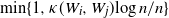 $\min\{1,\kappa(W_i,W_j){\log n}/{n}\}$
with
$\min\{1,\kappa(W_i,W_j){\log n}/{n}\}$
with
 $\kappa$
being a square-integrable kernel were studied in [Reference Devroye and Fraiman15]. Note that due to the dependency of
$\kappa$
being a square-integrable kernel were studied in [Reference Devroye and Fraiman15]. Note that due to the dependency of
 $\varepsilon$
in our
$\varepsilon$
in our
 $p_{ij}$
, this does not fall in this setting; as such, connectivity properties of this ensemble would deserve a new detailed analysis, which will be addressed elsewhere. We close this first rigorous work on this ensemble by pointing out that connectivity properties heavily depend on the
$p_{ij}$
, this does not fall in this setting; as such, connectivity properties of this ensemble would deserve a new detailed analysis, which will be addressed elsewhere. We close this first rigorous work on this ensemble by pointing out that connectivity properties heavily depend on the
 $\varepsilon$
regime considered, as can be already appreciated by looking at the presence of dust (i.e. isolated points in the graph). Indeed, the following and previous statements show a cross-over for the absence of dust at the
$\varepsilon$
regime considered, as can be already appreciated by looking at the presence of dust (i.e. isolated points in the graph). Indeed, the following and previous statements show a cross-over for the absence of dust at the
 $\varepsilon$
scale
$\varepsilon$
scale
 $(\log n/n)^{1/\alpha}$
.
$(\log n/n)^{1/\alpha}$
.
Proposition 2.1. (No-dust regime.) Consider the graph
 $\mathbf{G}_n(\alpha, \varepsilon)$
. Let
$\mathbf{G}_n(\alpha, \varepsilon)$
. Let
 $N_0$
be the number of isolated vertices, i.e.
$N_0$
be the number of isolated vertices, i.e.
 \begin{equation} N_0 = \sum_{i=1}^n \textbf {1} _{\{i \; \textrm{is isolated}\}}. \end{equation}
Then
 $\mathbb{E}[N_0] \sim n\mathbb{E}[\textrm{e}^{-(n-1)\Gamma(1-\alpha)\varepsilon^\alpha W_1^{\alpha}}]$
. In particular, if
$\mathbb{E}[N_0] \sim n\mathbb{E}[\textrm{e}^{-(n-1)\Gamma(1-\alpha)\varepsilon^\alpha W_1^{\alpha}}]$
. In particular, if
 $\varepsilon\downarrow 0$
and
$\varepsilon\downarrow 0$
and
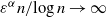 ${\varepsilon^{\alpha} n}/{\log n}\rightarrow \infty$
, then
${\varepsilon^{\alpha} n}/{\log n}\rightarrow \infty$
, then
 \begin{equation} \mathbb{P}(N_0=0)\to 1. \end{equation}
If
 $\varepsilon= n^{-1/\alpha}$
, then a positive fraction of points are isolated, i.e.
$\varepsilon= n^{-1/\alpha}$
, then a positive fraction of points are isolated, i.e.
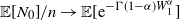 ${\mathbb{E}[N_0]}/{n} \rightarrow \mathbb{E}[\textrm{e}^{-\Gamma(1-\alpha) W_1^\alpha}]$
.
${\mathbb{E}[N_0]}/{n} \rightarrow \mathbb{E}[\textrm{e}^{-\Gamma(1-\alpha) W_1^\alpha}]$
.
3. The multi-scale model (MSM)
In this section we discuss the connection between our results and the model introduced in [Reference Garuccio, Lalli and Garlaschelli19].
3.1. Motivation for the MSM
The motivation for the MSM arises from statistical physics, where the concept of renormalization [Reference Kadanoff22, Reference Wilson39] plays a central role. In the context of networks, renormalization involves selecting a coarse-graining approach for a graph, which essentially means projecting a larger ‘microscopic’ graph onto a ‘reduced’ graph with fewer vertices [Reference Gabrielli, Garlaschelli, Patil and Serrano16]. This reduction is determined by a non-overlapping partition of the vertices of the original microscopic graph into ‘clusters’ or ‘supervertices’, which then become the vertices of the reduced graph. The edges of the reduced graph are defined according to specific rules, usually aimed at preserving certain structural features of the original network. This renormalization process can be iterated, potentially infinitely, in the case of an infinite graph.
For example, when the network is a regular lattice (or geometric graph) embedded in a specific metric space, a straightforward renormalization scheme exists. However, for generic (non-geometric) graphs, the absence of an explicit metric embedding makes the choice of renormalization significantly more challenging. Proposed approaches include borrowing box-covering techniques from fractal analysis [Reference Radicchi, Barrat, Fortunato and Ramasco25, Reference Song, Havlin and Makse29], employing spectral coarse-graining methods [Reference Gfeller and De Los Rios20, Reference Villegas, Gili, Caldarelli and Gabrielli38], and utilizing graph embedding techniques to infer optimal vertex coordinates in an imposed (usually hyperbolic) latent space [Reference Boguna, Bonamassa, De Domenico, Havlin, Krioukov and Serrano7, Reference Garca-Pérez, Boguñá and Serrano17]. For a recent review on network renormalization, see [Reference Gabrielli, Garlaschelli, Patil and Serrano16].
Regardless of the method used to find the optimal sequence of coarse-grainings for a given graph, the MSM has been introduced as a random graph model that remains consistently applicable to both the original graph and any reduced versions of it [Reference Garuccio, Lalli and Garlaschelli19]. This implies that, assuming the probability of generating a graph at the microscopic level follows a specific function of the model parameters, the probability of generating any reduced version of the graph should have the same functional form, potentially with renormalized parameters.
The MSM can be explicitly obtained as the model that fulfills the requirement that the random graph ensemble is scale-invariant under a renormalization process that accepts any partition of vertices. Importantly, this renormalization scheme is non-geometric by design, as it doesn’t rely on the notion of vertex coordinates in an underlying metric space, unlike the previously mentioned models based on the concept of geometric renormalization, where ‘closer’ vertices are merged.
3.2. Construction of the MSM
The renormalization framework allows for the same random graph ensemble to be observed at different hierarchical levels
 $\ell=0,1,2,\ldots$
. Let us start with the ‘microscopic’ level
$\ell=0,1,2,\ldots$
. Let us start with the ‘microscopic’ level
 $\ell=0$
and consider a random graph on
$\ell=0$
and consider a random graph on
 $n_0$
vertices where, adopting the notation used in [Reference Garuccio, Lalli and Garlaschelli19], each vertex (labeled as
$n_0$
vertices where, adopting the notation used in [Reference Garuccio, Lalli and Garlaschelli19], each vertex (labeled as
 $i_0=1,\ldots,n_0$
) has a weight
$i_0=1,\ldots,n_0$
) has a weight
 $X_{i_0}$
. To move to level
$X_{i_0}$
. To move to level
 $\ell=1$
, we specify a partition of the original
$\ell=1$
, we specify a partition of the original
 $n_0$
vertices into
$n_0$
vertices into
 $n_1{\lt \,}n_0$
blocks (which here, for simplicity, we assume to be all equal in size and composed of b vertices, so that
$n_1{\lt \,}n_0$
blocks (which here, for simplicity, we assume to be all equal in size and composed of b vertices, so that
 $n_1=n_0/b$
). The blocks of the partition, labeled
$n_1=n_0/b$
). The blocks of the partition, labeled
 $i_1=1,\ldots,n_1$
, become the vertices of the graph at the new level and each pair of blocks is connected if there existed at least an edge between any two original vertices placed across the two blocks. At this new level, the weights of all vertices inside a block
$i_1=1,\ldots,n_1$
, become the vertices of the graph at the new level and each pair of blocks is connected if there existed at least an edge between any two original vertices placed across the two blocks. At this new level, the weights of all vertices inside a block
 $i_1$
get summed to produce the (renormalized) weight for that block, denoted as
$i_1$
get summed to produce the (renormalized) weight for that block, denoted as
 $X_{i_1}\equiv \sum_{i_0\in i_1} X_{i_0}$
. The process can continue to higher levels
$X_{i_1}\equiv \sum_{i_0\in i_1} X_{i_0}$
. The process can continue to higher levels
 $\ell\, {\gt} 1$
by progressively reducing the graph to one with
$\ell\, {\gt} 1$
by progressively reducing the graph to one with
 $n_{\ell+1}=n_{\ell}/b=\cdots=n_0/b^{\ell+1}$
vertices and renormalizing the weights as
$n_{\ell+1}=n_{\ell}/b=\cdots=n_0/b^{\ell+1}$
vertices and renormalizing the weights as
 $X_{i_{\ell+1}}\equiv \sum_{i_{\ell}\in i_{\ell+1}} X_{i_{\ell}}$
.
$X_{i_{\ell+1}}\equiv \sum_{i_{\ell}\in i_{\ell+1}} X_{i_{\ell}}$
.
To define the MSM, we enforce the requirement that, under the coarse-graining process defined above, the probability distribution of the graph preserves the same functional form across all levels. This scale-invariant requirement becomes particularly simple if we consider the family of random graph models with independent edges, which are entirely specified by a function
 $p_{i_\ell j_\ell}$
of the parameters, representing the probability that the vertices
$p_{i_\ell j_\ell}$
of the parameters, representing the probability that the vertices
 $i_\ell$
and
$i_\ell$
and
 $j_\ell$
are connected. For this family, the connection probability
$j_\ell$
are connected. For this family, the connection probability
 $p_{i_{\ell+1} j_{\ell+1}}$
between two vertices
$p_{i_{\ell+1} j_{\ell+1}}$
between two vertices
 $i_{\ell+1}$
and
$i_{\ell+1}$
and
 $j_{\ell+1}$
defined at the level
$j_{\ell+1}$
defined at the level
 $\ell+1$
is related to the connection probabilities
$\ell+1$
is related to the connection probabilities
 $\{p_{i_\ell j_\ell}\}_{i_\ell,j_\ell}$
between the vertices at the previous level
$\{p_{i_\ell j_\ell}\}_{i_\ell,j_\ell}$
between the vertices at the previous level
 $\ell$
via
$\ell$
via
 \begin{equation} p_{i_{\ell+1} j_{\ell+1}}=1-\prod_{i_\ell\in i_{\ell+1}}\prod_{j_\ell\in j_{\ell+1}}(1-p_{i_\ell j_\ell}).\end{equation}
Assuming that the connection probability depends on a global parameter
 $\delta\, {\gt} \,0$
as well as on the additive vertex weights
$\delta\, {\gt} \,0$
as well as on the additive vertex weights
 $\{X_{i_\ell}\}_{i_\ell}$
introduced above, the simplest non-trivial expression consistent with (3.1) is given by
$\{X_{i_\ell}\}_{i_\ell}$
introduced above, the simplest non-trivial expression consistent with (3.1) is given by
 \begin{equation} p_{i_\ell j_\ell} = 1 - \exp \! ({-\delta X_{i_\ell} X_{j_\ell}}).\end{equation}
At this point, we may require that the weights are either deterministic parameters assigned to the vertices, so that the only source of randomness lies in the realization of the graph (‘quenched’ variant of the MSM), or that they are random variables themselves, thus adding a second layer of randomness (‘annealed’ variant of the MSM). In the latter case, it is natural to subject the weights to the same scale-invariant requirement as the random graph, i.e. to demand that the weights are drawn from the same probability density function (with possibly renormalized parameters) at all hierachical levels. Since the weights are chosen to be additive upon renormalization, this requirement immediately implies that they must be drawn from an
 $\alpha$
-stable distribution. Moreover, the positivity of the weights and the concurrent requirement that the support of their pdf is the non-negative real axis, irrespective of the hierarchical level, imply that they should be one-sided
$\alpha$
-stable distribution. Moreover, the positivity of the weights and the concurrent requirement that the support of their pdf is the non-negative real axis, irrespective of the hierarchical level, imply that they should be one-sided
 $\alpha$
-stable random variables with (scale-invariant) parameter
$\alpha$
-stable random variables with (scale-invariant) parameter
 $\alpha\in(0,1)$
and some (scale-dependent) scale parameter
$\alpha\in(0,1)$
and some (scale-dependent) scale parameter
 $\gamma_\ell$
. In this way, if the blocks of the partition are always of size b, as assumed above, then the vertex weights at level
$\gamma_\ell$
. In this way, if the blocks of the partition are always of size b, as assumed above, then the vertex weights at level
 $\ell$
are one-sided
$\ell$
are one-sided
 $\alpha$
-stable random variables with rescaled parameter
$\alpha$
-stable random variables with rescaled parameter
 $\gamma_{\ell} = b^{1/\alpha} \gamma_{\ell-1}=\cdots=b^{\ell/\alpha} \gamma_{0}=(n_0/n_\ell)^{1/\alpha}\gamma_0$
. This completes the definition of the annealed MSM, along with its renormalization rules for both the weights of vertices and all the other model parameters.
$\gamma_{\ell} = b^{1/\alpha} \gamma_{\ell-1}=\cdots=b^{\ell/\alpha} \gamma_{0}=(n_0/n_\ell)^{1/\alpha}\gamma_0$
. This completes the definition of the annealed MSM, along with its renormalization rules for both the weights of vertices and all the other model parameters.
3.3. Connection between the MSM and the model studied in this paper
Despite the obvious relationship between the model studied in this paper and the original annealed version of the MSM recalled above (in particular, between (1.1) and (3.2)), there are apparently some differences that require further discussion. First, here we have considered weights drawn from a Pareto distribution with tail exponent
 $\alpha$
, rather than a one-sided
$\alpha$
, rather than a one-sided
 $\alpha$
-stable distribution; second, here the other parameters of the weight distribution are fixed and the scale parameter
$\alpha$
-stable distribution; second, here the other parameters of the weight distribution are fixed and the scale parameter
 $\varepsilon$
is n-dependent, while in the original model the other parameters (
$\varepsilon$
is n-dependent, while in the original model the other parameters (
 $\gamma$
) of the weight distribution are
$\gamma$
) of the weight distribution are
 $\ell$
-dependent (hence also n-dependent) and the scale parameter
$\ell$
-dependent (hence also n-dependent) and the scale parameter
 $\delta$
is fixed; third, here we have not exploited the scale-invariant nature of the MSM under coarse-graining. We now clarify the close relationship between the two variants of the model, these apparent differences notwithstanding.
$\delta$
is fixed; third, here we have not exploited the scale-invariant nature of the MSM under coarse-graining. We now clarify the close relationship between the two variants of the model, these apparent differences notwithstanding.
Let us start by recalling that, for large values of the argument x, a one-sided
 $\alpha$
-stable distribution
$\alpha$
-stable distribution
 $\mathbb{P}(X\, {\gt} \,x)$
with scale parameter
$\mathbb{P}(X\, {\gt} \,x)$
with scale parameter
 $\gamma$
is well approximated by a pure power-law (Pareto) distribution
$\gamma$
is well approximated by a pure power-law (Pareto) distribution
 $\mathbb{P}(X\, {\gt} \,x)\sim C_{\alpha,\gamma} \; x^{-\alpha}$
with a prefactor
$\mathbb{P}(X\, {\gt} \,x)\sim C_{\alpha,\gamma} \; x^{-\alpha}$
with a prefactor
 $C_{\alpha,\gamma}$
that depends on the parameters of the stable law [Reference Samorodnitsky and Taqqu28]:
$C_{\alpha,\gamma}$
that depends on the parameters of the stable law [Reference Samorodnitsky and Taqqu28]:
 \begin{equation} C_{\alpha,\gamma} \equiv \gamma^{\alpha}c_\alpha, \qquad\text{with } c_\alpha \equiv \frac{2\Gamma({\alpha})}{\pi}\sin{\frac{\pi\alpha}{2}}.\end{equation}
Then, we note that, besides
 $n_0$
and b, the three remaining parameters of the original annealed MSM are
$n_0$
and b, the three remaining parameters of the original annealed MSM are
 $\alpha\in(0,1)$
,
$\alpha\in(0,1)$
,
 $\gamma_0\in(0,\infty)$
, and
$\gamma_0\in(0,\infty)$
, and
 $\delta\in(0,\infty)$
. However, of these three parameters, only
$\delta\in(0,\infty)$
. However, of these three parameters, only
 $\alpha$
and the combination
$\alpha$
and the combination
 $\delta \gamma_0^2$
are independent. Indeed, it is easy to realize that rescaling
$\delta \gamma_0^2$
are independent. Indeed, it is easy to realize that rescaling
 $\gamma_0$
to
$\gamma_0$
to
 $\gamma_0/\lambda$
(which is equivalent to rescaling
$\gamma_0/\lambda$
(which is equivalent to rescaling
 $X_{i_\ell}$
to
$X_{i_\ell}$
to
 $X_{i_\ell}/\lambda$
, for some
$X_{i_\ell}/\lambda$
, for some
 $\lambda\, {\gt} \,0$
) while simultaneously rescaling
$\lambda\, {\gt} \,0$
) while simultaneously rescaling
 $\delta$
to
$\delta$
to
 $\lambda^{2}\delta$
leaves the connection probability unchanged. In combination with the scale-invariant nature of the MSM, this property can be exploited to map the quantities
$\lambda^{2}\delta$
leaves the connection probability unchanged. In combination with the scale-invariant nature of the MSM, this property can be exploited to map the quantities
 $(\{X_{i_\ell}\}_{i_\ell=1}^{n_\ell},\delta)$
introduced in the original model to the quantities
$(\{X_{i_\ell}\}_{i_\ell=1}^{n_\ell},\delta)$
introduced in the original model to the quantities
 $(\{W_{i}\}_{i=1}^{n}, \varepsilon)$
used here by choosing a level
$(\{W_{i}\}_{i=1}^{n}, \varepsilon)$
used here by choosing a level
 $\ell$
such that the number
$\ell$
such that the number
 $n_\ell$
of vertices in the MSM equals the one desired here, i.e.
$n_\ell$
of vertices in the MSM equals the one desired here, i.e.
 $n=n_\ell$
, and defining the weight of vertex i as
$n=n_\ell$
, and defining the weight of vertex i as
 $W_{i} \equiv c_{\alpha}^{-1/\alpha}\gamma_\ell^{-1} X_{i_\ell} $
for
$W_{i} \equiv c_{\alpha}^{-1/\alpha}\gamma_\ell^{-1} X_{i_\ell} $
for
 $i=1,\ldots,n$
, so that
$i=1,\ldots,n$
, so that
 \begin{equation} \lim_{x \to \infty}\mathbb{P}(W_{i} \, {\gt} \, x) \; x^{\alpha} = 1, \quad i=1,\ldots,n,\end{equation}
irrespective of
 $\ell$
. This implies that, while the distribution of
$\ell$
. This implies that, while the distribution of
 $X_{i_\ell}$
depends on
$X_{i_\ell}$
depends on
 $\ell$
through the parameter
$\ell$
through the parameter
 $\gamma_\ell$
(see (3.3)), the distribution of
$\gamma_\ell$
(see (3.3)), the distribution of
 $W_{i}$
is actually
$W_{i}$
is actually
 $\ell$
-independent in the tail, which is why we could drop the subscript
$\ell$
-independent in the tail, which is why we could drop the subscript
 $\ell$
in redefining
$\ell$
in redefining
 $W_{i}$
. Note that this procedure yields weights that are only asymptotically
$W_{i}$
. Note that this procedure yields weights that are only asymptotically
 $\ell$
-independent, as expressed in (3.4). Nevertheless, in this way we can keep the connection probability unchanged (i.e.
$\ell$
-independent, as expressed in (3.4). Nevertheless, in this way we can keep the connection probability unchanged (i.e.
 $1-\textrm{e}^{-\delta X_{i_\ell} X_{j_\ell}} \equiv 1-\textrm{e}^{-\varepsilon_{n_\ell} W_{i} W_{j}}$
) while moving the scale-dependence from
$1-\textrm{e}^{-\delta X_{i_\ell} X_{j_\ell}} \equiv 1-\textrm{e}^{-\varepsilon_{n_\ell} W_{i} W_{j}}$
) while moving the scale-dependence from
 $\{X_{i_\ell}\}_{i_\ell=1}^{n_\ell}$
to
$\{X_{i_\ell}\}_{i_\ell=1}^{n_\ell}$
to
 $\varepsilon_{n_\ell}$
by redefining the latter in one of the following equivalent ways:
$\varepsilon_{n_\ell}$
by redefining the latter in one of the following equivalent ways:
 \begin{equation} \varepsilon_{n_\ell} \equiv c_{\alpha}^{2/\alpha}\gamma_{\ell}^{2}\delta = c_{\alpha}^{2/\alpha}\bigg(\frac{n_0}{n_\ell}\bigg)^{2/\alpha}\gamma_0^2\delta = c_{\alpha}^{2/\alpha}b^{2\ell/\alpha}\gamma_0^2\delta = b^{2\ell/\alpha}\varepsilon_{n_0}, \qquad \text{where}\ \varepsilon_{n_0} \equiv c_{\alpha}^{2/\alpha} \gamma_{0}^{2}\delta,\end{equation}
where we now make explicit the dependence of
 $\varepsilon$
on
$\varepsilon$
on
 $n_\ell$
to track variations across scales
$n_\ell$
to track variations across scales
 $\ell$
. In other words, our formulation here can be thought of as deriving from an equivalent MSM where, rather than having a scale-dependent fitness distribution and a scale-independent global parameter
$\ell$
. In other words, our formulation here can be thought of as deriving from an equivalent MSM where, rather than having a scale-dependent fitness distribution and a scale-independent global parameter
 $\delta$
, we have a scale-independent fitness distribution (with asymptotically the same tail as the Pareto in (2.1)) and a scale-dependent global parameter
$\delta$
, we have a scale-independent fitness distribution (with asymptotically the same tail as the Pareto in (2.1)) and a scale-dependent global parameter
 $\varepsilon_{n}=\varepsilon_{n_\ell}$
, for an implied hierarchical level
$\varepsilon_{n}=\varepsilon_{n_\ell}$
, for an implied hierarchical level
 $\ell$
. According to (3.5), since
$\ell$
. According to (3.5), since
 $\delta$
,
$\delta$
,
 $\alpha$
, and b are finite constants, achieving a certain scaling of
$\alpha$
, and b are finite constants, achieving a certain scaling of
 $\varepsilon_n$
with n in the model considered here corresponds to achieving a corresponding scaling of
$\varepsilon_n$
with n in the model considered here corresponds to achieving a corresponding scaling of
 $\gamma_\ell$
with
$\gamma_\ell$
with
 $n_\ell$
(or equivalently of
$n_\ell$
(or equivalently of
 $\gamma_0$
with
$\gamma_0$
with
 $n_0$
), or ultimately to finding an appropriate
$n_0$
), or ultimately to finding an appropriate
 $\ell$
, in the original model. Results that we obtain for a specific range of values of
$\ell$
, in the original model. Results that we obtain for a specific range of values of
 $\varepsilon$
can therefore be thought of as applying to a corresponding specific range of hierarchical levels in the original model. In particular, Theorems 2.1 and 2.2 reveal that at the specific scale
$\varepsilon$
can therefore be thought of as applying to a corresponding specific range of hierarchical levels in the original model. In particular, Theorems 2.1 and 2.2 reveal that at the specific scale
 $\varepsilon = \lambda n^{-1/\alpha}$
the model undergoes drastic structural changes (e.g. concerning typical degrees and wedges).
$\varepsilon = \lambda n^{-1/\alpha}$
the model undergoes drastic structural changes (e.g. concerning typical degrees and wedges).
3.4. Implications of our results for the MSM
Some topological properties of the original MSM were investigated in [Reference Garuccio, Lalli and Garlaschelli19] numerically, and either analytically (for
 $\alpha = \frac12$
, corresponding to the Lévy distribution, which is the only one-sided
$\alpha = \frac12$
, corresponding to the Lévy distribution, which is the only one-sided
 $\alpha$
-stable distribution that can be written in explicit form) or semi-analytically (for generic
$\alpha$
-stable distribution that can be written in explicit form) or semi-analytically (for generic
 $\alpha\in (0,1)$
). Notably, it was found that networks sampled from the MSM feature an empirical degree distribution P(k) exhibiting a scale-free region, characterized by a universal power-law decay
$\alpha\in (0,1)$
). Notably, it was found that networks sampled from the MSM feature an empirical degree distribution P(k) exhibiting a scale-free region, characterized by a universal power-law decay
 $\propto k^{-2}$
(corresponding to a cumulative distribution with decay
$\propto k^{-2}$
(corresponding to a cumulative distribution with decay
 $\propto k^{-1}$
) irrespective of the value of
$\propto k^{-1}$
) irrespective of the value of
 $\alpha\in(0,1)$
, followed by a density-dependent cut-off.
$\alpha\in(0,1)$
, followed by a density-dependent cut-off.
The results obtained here provide significant additional insights. With regard to the degrees, we have identified the specific scaling (or equivalently, as explained in Section 3.3, the specific hierarchical level) for which the density-dependent cut-off disappears and the tail of the cumulative degree distribution can be rigorously proven (through an independent proof) to become a pure power law with exponent
 $-1$
, for any
$-1$
, for any
 $\alpha \in (0,1)$
. Secondly, we have provided a rigorous evaluation of the overall number of triangles and wedges, valid for any
$\alpha \in (0,1)$
. Secondly, we have provided a rigorous evaluation of the overall number of triangles and wedges, valid for any
 $\alpha$
, that supports the outcome of simulations shown in the original paper, which illustrated the vanishing of the global clustering coefficient in the sparse limit (as opposed to the local clustering coefficient, which remains bounded away from zero as recalled above).
$\alpha$
, that supports the outcome of simulations shown in the original paper, which illustrated the vanishing of the global clustering coefficient in the sparse limit (as opposed to the local clustering coefficient, which remains bounded away from zero as recalled above).
4. Proof of Theorem 2.1: Typical degrees
Since Karamata’s Tauberian theorem is used here as a key tool in the analysis of the degree distribution and later analysis, it is first worth recalling those results.
Theorem 4.1. (Karamata’s Tauberian theorem [Reference Bingham, Goldie, Teugels and Teugels6, Theorem 8.1.6].) Let X be a non-negative random variable with distribution F and Laplace transform
 $\widehat F(s) = \mathbb{E}[\textrm{e}^{-sX}]$
,
$\widehat F(s) = \mathbb{E}[\textrm{e}^{-sX}]$
,
 $s\ge 0$
. Let L be a slowly varying function and
$s\ge 0$
. Let L be a slowly varying function and
 $\alpha\in (0,1)$
; then the following are equivalent:
$\alpha\in (0,1)$
; then the following are equivalent:
 \begin{align*} 1 - \widehat F(s) & \sim \Gamma(1-\alpha)s^{\alpha}L({1}/{s}) \quad \text{ $as \ s\downarrow 0$}, \\ 1 - F(x) & \sim x^{-\alpha} L(x) \quad \text{ $ as \ x\to \infty$}. \end{align*}
Then, another property of the tails of products of regularly varying distributions will be needed. A general statement about the product of n independent and identically distributed (i.i.d.) random variables with Pareto tails can be found in [Reference Anders Hedegaard Jessen1, Lemma 4.1 (4)]. For completeness, a proof for two random variables is given here, which is useful in our analysis.
Lemma 4.1. Let
 $W_1$
and
$W_1$
and
 $W_2$
be independent random variables satisfying the tail assumptions (2.1). Then
$W_2$
be independent random variables satisfying the tail assumptions (2.1). Then
 $\mathbb{P}(W_1W_2 \ge x) \sim \alpha x^{-\alpha}\log x$
as
$\mathbb{P}(W_1W_2 \ge x) \sim \alpha x^{-\alpha}\log x$
as
 $x \to \infty$
.
$x \to \infty$
.
Proof. Consider the random variable
 $\log(W_1)$
, which follows an exponential distribution, or alternatively a Gamma distribution with shape parameter
$\log(W_1)$
, which follows an exponential distribution, or alternatively a Gamma distribution with shape parameter
 $k=1$
and scale
$k=1$
and scale
 $\theta = 1/\alpha$
. Then, the random variable
$\theta = 1/\alpha$
. Then, the random variable
 $Z = \log(W_1) + \log(W_2)$
follows a Gamma distribution with shape parameter 2 and scale
$Z = \log(W_1) + \log(W_2)$
follows a Gamma distribution with shape parameter 2 and scale
 $\theta$
. This means that
$\theta$
. This means that
 \begin{equation*} \mathbb{P}(\log(W_1) + \log(W_2) \, {\gt} \, x) = \frac{\alpha^2}{\Gamma(2)}\int_{x}^{\infty}y\textrm{e}^{-\alpha y}\,\textrm{d} y. \end{equation*}
Therefore
 \begin{equation} \mathbb{P}(W_1W_2 \, {\gt} \, x) = \mathbb{P}(\log{W_1} + \log{W_2} \, {\gt} \, \log{x}) = \alpha^2\int_{\log{x}}^{\infty}y\textrm{e}^{-\alpha y}\,\textrm{d} y = \alpha^2\int_{x}^{\infty}\log(t)t^{-\alpha-1}\,\textrm{d} t. \end{equation}
Then, applying Karamata’s theorem (see [Reference Anders Hedegaard Jessen1, Theorem 12]),
 \begin{equation*} \mathbb{P}(W_1W_2 \, {\gt} \, x) \sim \alpha^2\,\frac{x^{-\alpha}\log{x}}{\alpha}, \end{equation*}
which proves the statement.
Remark 4.1. Theorem 4.1 remains true if
 $W_1$
and
$W_1$
and
 $W_2$
are not exactly Pareto, but asymptotically tail-equivalent to a Pareto distribution, i.e. under the assumption
$W_2$
are not exactly Pareto, but asymptotically tail-equivalent to a Pareto distribution, i.e. under the assumption
 $\mathbb{P}(W_1\, {\gt} \,x) \sim cx^{-\alpha}$
as
$\mathbb{P}(W_1\, {\gt} \,x) \sim cx^{-\alpha}$
as
 $x\to \infty$
. See [Reference Anders Hedegaard Jessen1, Lemma 4.1] for a proof.
$x\to \infty$
. See [Reference Anders Hedegaard Jessen1, Lemma 4.1] for a proof.
Proof of Theorem 2.1 . For (i), we begin by evaluating the asymptotics of the expected degree, which is an easy consequence of Lemma 4.1 and Theorem 4.1. Indeed, we can write
 \begin{equation} \mathbb{E}[D_n(i)] = \sum_{j \neq i}\mathbb{E}[1 - \exp \! (\!-\!\varepsilon W_iW_j)] = (n-1)\mathbb{E}[1 - \exp \! (\!-\!\varepsilon W_1W_2)], \end{equation}
where the last equality is due to the i.i.d. nature of the weights. It follows from Lemma 4.1 that
 $\mathbb{P}(W_1W_2\, {\gt} \, x) \sim \alpha x^{-\alpha}\log{x}$
. Therefore, using Theorem 4.1, we have
$\mathbb{P}(W_1W_2\, {\gt} \, x) \sim \alpha x^{-\alpha}\log{x}$
. Therefore, using Theorem 4.1, we have
 \begin{equation*} \mathbb{E}[1 - \exp \! (\!-\!\varepsilon W_1W_2)] \sim \Gamma(1-\alpha)\alpha\varepsilon^{\alpha}\log\frac{1}{\varepsilon} \quad \text{as $\varepsilon\downarrow 0$}, \end{equation*}
which together with (4.2) gives the claim.
For (ii), by following the line of the proof of [Reference van der Hofstad32, Theorem 6.14], we can prove our statement by showing that the probability-generating function of
 $D_n(i)$
in the limit
$D_n(i)$
in the limit
 $n \to \infty$
corresponds to the probability-generating function of a mixed Poisson random variable. Let
$n \to \infty$
corresponds to the probability-generating function of a mixed Poisson random variable. Let
 $t\in (0,1)$
; the probability-generating function of the degree
$t\in (0,1)$
; the probability-generating function of the degree
 $D_n(i)$
reads
$D_n(i)$
reads
 \begin{equation*} \mathbb{E}\big[t^{D_n(i)}\big] = \mathbb{E}\big[t^{\sum_{j \neq i}a_{ij}}\big] = \mathbb{E}\Bigg[\prod_{j \neq i}t^{ a_{ij}}\Bigg], \end{equation*}
where
 $a_{ij}$
are the entries of the adjacency matrix related to the graph
$a_{ij}$
are the entries of the adjacency matrix related to the graph
 $\mathbf{G}_n(\alpha, \varepsilon)$
, i.e. Bernoulli random variables with parameter
$\mathbf{G}_n(\alpha, \varepsilon)$
, i.e. Bernoulli random variables with parameter
 $p_{ij}$
as in (2.2). Conditioned on the weights, these variables are independent. Recall that we denoted by
$p_{ij}$
as in (2.2). Conditioned on the weights, these variables are independent. Recall that we denoted by
 $\mathbb{E}_{W_i}[\! \cdot \!]$
the conditional expectation given the weight
$\mathbb{E}_{W_i}[\! \cdot \!]$
the conditional expectation given the weight
 $W_i$
. Then
$W_i$
. Then
 \begin{align*} \mathbb{E}_{W_i}\big[t^{D_n(i)}\big] = \mathbb{E}_{W_i}\Bigg[\prod_{j \neq i}\big((1-t)\textrm{e}^{-\varepsilon W_j W_i } + t\big)\Bigg] & = \prod_{j \neq i}\mathbb{E}_{W_i}\big[(1-t)\textrm{e}^{-\varepsilon W_j W_i} + t\big] \\ & = \prod_{j \neq i}\mathbb{E}_{W_i}[\varphi_{W_i}(\varepsilon W_j)], \end{align*}
where we have used the independence of the weights and introduced the function
 \begin{align*}\varphi_{W_{i}}(x) \;:\!=\; (1-t)\textrm{e}^{-W_i x} + t .\end{align*}
To simplify our expression we introduce the notation
 $\psi_n(W_{i}) \;:\!=\; \mathbb{E}_{W_i}[\varphi_{W_{i}}(\varepsilon W_j)]$
for some
$\psi_n(W_{i}) \;:\!=\; \mathbb{E}_{W_i}[\varphi_{W_{i}}(\varepsilon W_j)]$
for some
 $j\neq i$
. Using exchangeability and the tower property of the conditional expectation, the moment-generating function of
$j\neq i$
. Using exchangeability and the tower property of the conditional expectation, the moment-generating function of
 $D_n(i)$
can be written as
$D_n(i)$
can be written as
 \begin{equation} \mathbb{E}[t^{D_n(i)}] = \mathbb{E}\Bigg[\prod_{j \neq i}\mathbb{E}_{W_i}[\varphi_{W_{i}}(\varepsilon W_j)]\Bigg] = \mathbb{E}[\psi_n(W_{i})^{n-1}]. \end{equation}
Consider now a differentiable function
 $h\colon[0,\infty) \to \mathbb{R}$
such that
$h\colon[0,\infty) \to \mathbb{R}$
such that
 $h(0) = 0$
. By integration by parts, we can show that
$h(0) = 0$
. By integration by parts, we can show that
 \begin{equation} \mathbb{E}[h(W_j)] = \int_0^{\infty}h'(x)\mathbb{P}(W_j \, {\gt} \,x)\,\textrm{d} x. \end{equation}
By using (4.4) with
 $h(w) = \varphi_{W_i}(\varepsilon w) - 1$
, we have
$h(w) = \varphi_{W_i}(\varepsilon w) - 1$
, we have
 \begin{align} \psi_n(W_{i}) & = 1 + \mathbb{E}[\varphi_{W_{i}}(\varepsilon w) - 1] \nonumber \\ & = 1 + \int_0^{\infty}\varepsilon\varphi'_{W_{i}}(\varepsilon w)(1 - F_{W}(w))\,\textrm{d} w \nonumber \\ & = 1 + \int_0^{\infty}\varphi'_{W_{i}}(y)(1 - F_{W}(\varepsilon^{-1}y))\,\textrm{d} y \nonumber \\ & = 1 + \int_0^{\varepsilon}\varphi'_{W_{i}}(y)\,\textrm{d} y + \int_{\varepsilon}^\infty\varphi'_{W_{i}}(y)(1 - F_{W}(\varepsilon^{-1} y))\,\textrm{d} y \nonumber \\ & = 1 + \varphi_{W_i}(\varepsilon) - \varphi_{W_i}(0) + \varepsilon^{\alpha}\int_{\varepsilon}^\infty(t-1)W_{i}\textrm{e}^{-yW_{i}}y^{-\alpha}\,\textrm{d} y. \end{align}
In particular, for
 $\varepsilon=n^{-1/\alpha}$
, combining (4.3) and (4.5) gives
$\varepsilon=n^{-1/\alpha}$
, combining (4.3) and (4.5) gives
 \begin{align*} \mathbb{E}\big[t^{D_n(i)}\big] & = \mathbb{E}[\psi_n(W_i)^{n-1}] \\ & = \mathbb{E}\bigg[\bigg(1 + \varphi_{W_i}(n^{-1/\alpha}) - \varphi_{W_i}(0) + \frac{1}{n}\int_{n^{-1/\alpha}}^\infty(t-1)W_{i}\textrm{e}^{-yW_{i}}y^{-\alpha}\,\textrm{d} y\bigg)^{n-1}\bigg]. \end{align*}
Note that for a fixed realization of
 $W_i$
, using the change of variable
$W_i$
, using the change of variable
 $z= W_i y$
we have, as
$z= W_i y$
we have, as
 $n\to \infty$
,
$n\to \infty$
,
 \begin{align*}(1-t)\int_{n^{-1/\alpha}}^\infty W_{i}\textrm{e}^{-yW_{i}}y^{-\alpha}\,\textrm{d} y \to (1-t)W_i^\alpha\Gamma(1-\alpha)\end{align*}
and
 $\varphi_{W_i}(n^{-1/\alpha})\to \varphi_{W_i}(0)=1$
.
$\varphi_{W_i}(n^{-1/\alpha})\to \varphi_{W_i}(0)=1$
.
Observe that
 $\varphi_{W_i}(n^{-1/\alpha})-\varphi(0)= -(1-t)\big(1-\textrm{e}^{-W_in^{1/\alpha}}\big)\le 0$
and
$\varphi_{W_i}(n^{-1/\alpha})-\varphi(0)= -(1-t)\big(1-\textrm{e}^{-W_in^{1/\alpha}}\big)\le 0$
and
 \begin{align*}0\le (1-t)\int_{n^{-1/\alpha}}^\infty W_{i}\textrm{e}^{-yW_{i}}y^{-\alpha}\,\textrm{d} y \le (1-t)W_i^{\alpha}\Gamma(1-\alpha).\end{align*}
Hence, using
 $(1-x/n)^n \le \textrm{e}^{-x}$
we have
$(1-x/n)^n \le \textrm{e}^{-x}$
we have
 \begin{align*} &\bigg(1 + \varphi_{W_i}(n^{-1/\alpha}) - \varphi_{W_i}(0) - (1-t)\frac{1}{n}\int_{n^{-1/\alpha}}^\infty W_{i}\textrm{e}^{-yW_{i}}y^{-\alpha}\,\textrm{d} y\bigg)^{n-1}\\ &\quad \le \exp\big({-}(1-t)W_i^{\alpha}\Gamma(1-\alpha)\big) \le 1. \end{align*}
Thus, we can apply the dominated convergence theorem to claim that
 \begin{align*} \lim_{n\to\infty}\mathbb{E}\big[t^{D_n(i)}\big] = \mathbb{E}[\exp \! (\!-\!(1-t)\,W_i^{\alpha}\Gamma(1-\alpha))], \end{align*}
so the generating function of the graph degree
 $D_n(i)$
asymptotically corresponds to the generating function of a mixed Poisson random variable with parameter
$D_n(i)$
asymptotically corresponds to the generating function of a mixed Poisson random variable with parameter
 $\Gamma(1-\alpha)W_i^{\alpha}$
. Therefore, the variable
$\Gamma(1-\alpha)W_i^{\alpha}$
. Therefore, the variable
 $D_n(i)\overset{\textrm{d}}\rightarrow D_{\infty}(i)$
, where
$D_n(i)\overset{\textrm{d}}\rightarrow D_{\infty}(i)$
, where
 $D_{\infty}(i) \mid W_i \overset{\textrm{d}}= \operatorname{Poisson} \! (\Gamma(1-\alpha)W_i^{\alpha})$
.
$D_{\infty}(i) \mid W_i \overset{\textrm{d}}= \operatorname{Poisson} \! (\Gamma(1-\alpha)W_i^{\alpha})$
.
In particular, we have the following tail of the distribution of the random variable
 $D_{\infty}(i)$
:
$D_{\infty}(i)$
:
 \begin{align*} \mathbb{P}(D_{\infty}(i) \ge k) & = \int_0^{\infty}\mathbb{P}\big(\operatorname{Poisson} \! (\Gamma(1-\alpha) w^{\alpha}) \ge k \mid W_i = w\big)\,F_{W_i}(\textrm{d} w) \\ & = \int_0^{\infty}\sum_{m\ge k}\frac{\textrm{e}^{-\Gamma(1-\alpha)w^\alpha}\Gamma(1-\alpha)^{m}w^{\alpha m}}{m!}\,F_{W_i}(\textrm{d} w) \\ & = \sum_{m\ge k}\frac{1}{m!}\int_1^{\infty}\textrm{e}^{-\Gamma(1-\alpha)w^\alpha}\Gamma(1-\alpha)^{m}w^{\alpha m} \alpha w^{-\alpha-1}\,\textrm{d} w. \end{align*}
Introducing the new variable
 $y = \Gamma(1-\alpha)w^\alpha$
, we have
$y = \Gamma(1-\alpha)w^\alpha$
, we have
 \begin{align} & \int_1^{\infty}\textrm{e}^{-\Gamma(1-\alpha)w^\alpha}\Gamma(1-\alpha)^{m}w^{\alpha m}\alpha w^{-\alpha-1}\,\textrm{d} w \nonumber \\ & \qquad = \int_{1}^\infty\textrm{e}^{-\Gamma(1-\alpha)w^\alpha}\Gamma(1-\alpha)^{m-1}w^{\alpha m}w^{-2\alpha}\alpha\Gamma(1-\alpha) w^{\alpha-1}\,\textrm{d} w \nonumber \\ & \qquad = \Gamma(1-\alpha)\int_{\Gamma(1-\alpha)}^\infty\textrm{e}^{-y}y^{m-2}\,\textrm{d} y \nonumber \\ & \qquad = \Gamma(1-\alpha)\Gamma(m-1) - \Gamma(1-\alpha)\int_0^{\Gamma(1-\alpha)}\textrm{e}^{-y}y^{m-2}\,\textrm{d} y. \end{align}
The first integral is dominant with respect to the second one. To show this, we can use a trivial bound:
 \begin{align*}\int_0^{\Gamma(1-\alpha)}\textrm{e}^{-y}y^{m-2}\,\textrm{d} y \leq \Gamma(1-\alpha)^{m}.\end{align*}
Since
 $m! \ge (m/\textrm{e})^m$
, the following inequalities hold true:
$m! \ge (m/\textrm{e})^m$
, the following inequalities hold true:
 \begin{align*} \sum_{m\ge k}\frac{\Gamma(1-\alpha)^m}{m!} \le \sum_{m\ge k}\frac{(\textrm{e}\Gamma(1-\alpha))^m}{m^m} \le C(\textrm{e}\Gamma(1-\alpha))^k k^{-k} \end{align*}
for some positive constant C. Note that in last step we used the fact that k is large enough (it is at least greater that
 $\textrm{e}\Gamma(1-\alpha)$
). Note that
$\textrm{e}\Gamma(1-\alpha)$
). Note that
 \begin{align*} k\sum_{m\ge k}\frac{\Gamma(1-\alpha)^m}{m!} \le C\textrm{e}^{\log k - k\log k + k\textrm{e}\Gamma(1-\alpha)} \to 0 \quad \text{as $k\to \infty$}. \end{align*}
Using (4.6), we therefore obtain
 \begin{align*} \sum_{m\ge k}\frac{1}{m!}\int_1^{\infty}\textrm{e}^{-\Gamma(1-\alpha)w^\alpha}\Gamma(1-\alpha)^{m}w^{\alpha m} \alpha w^{-\alpha-1}\,\textrm{d} w & = \Gamma(1-\alpha)\sum_{m\ge k}\frac{\Gamma(m-1)}{m!} + o(k^{-1}) \\ & = \Gamma(1-\alpha)\sum_{m\ge k}\frac{(m-2)!}{m!} + o(k^{-1}) \\ & = \Gamma(1-\alpha)\sum_{m\ge k}\frac{1}{m(m-1)} + o(k^{-1}) \\ & \sim \frac{\Gamma(1-\alpha)}{k}. \end{align*}
This shows that
 $\mathbb{P}(D_\infty(i)\ge k) \sim \Gamma(1-\alpha)k^{-1}$
as
$\mathbb{P}(D_\infty(i)\ge k) \sim \Gamma(1-\alpha)k^{-1}$
as
 $k\to\infty$
.
$k\to\infty$
.
For (iii), fix
 $t,s\in(0,1)$
. Due to the exchangeability of vertices, without loss of generality we just consider vertices 1 and 2:
$t,s\in(0,1)$
. Due to the exchangeability of vertices, without loss of generality we just consider vertices 1 and 2:
 \begin{align} & \mathbb{E}\big[t^{D_{n}(1)}s^{D_n(2)}\big] \nonumber \\ & \qquad = \mathbb{E}\big[t^{\sum_{j \neq 1}a_{1j}}s^{\sum_{j \neq 2}a_{2j}}\big] \nonumber \\ & \qquad = \mathbb{E}\Bigg[\prod_{j \neq 1,2}t^{a_{1j}}s^{a_{2j}}(ts)^{a_{12}}\Bigg] \nonumber \\ & \qquad = \mathbb{E}\Bigg[\big((1-ts)\textrm{e}^{-\varepsilon W_1 W_2} + ts\big) \prod_{j \neq 1,2}\big((1-t)\textrm{e}^{-\varepsilon W_1 W_j} + t\big)\big((1-s)\textrm{e}^{-\varepsilon W_2 W_j} + s\big)\Bigg], \end{align}
where we have used the independence of the connection probabilities given the weights. In order to simplify the notation, we can introduce the functions
 \begin{align*} \phi_{a}^{b}(x) & \;:\!=\; (1 - b)\textrm{e}^{-\varepsilon ax} + b, \\ \psi_n(W_1,W_2) & \;:\!=\; \mathbb{E}_{W_1,W_2}\big[\phi_{W_1}^{t}(W_j)\phi_{W_2}^{s}(W_j)\big] \quad \text{for some $j \neq 1, 2$}, \end{align*}
where
 $a, b\, {\gt} \,0$
and, as customary throughout this paper,
$a, b\, {\gt} \,0$
and, as customary throughout this paper,
 $\mathbb{E}_{W_1,W_2}[\! \cdot \!] \;:\!=\; \mathbb{E}[\,\cdot \mid W_1,W_2]$
.
$\mathbb{E}_{W_1,W_2}[\! \cdot \!] \;:\!=\; \mathbb{E}[\,\cdot \mid W_1,W_2]$
.
Using the tower property of conditional expectation, (4.7) reads
 \begin{align*} \mathbb{E}\big[t^{D_n(1)}s^{D_n(2)}\big] & = \mathbb{E}\Bigg[\phi_{W_1}^{ts}(W_2)\prod_{j \neq 1,2}\phi_{W_1}^{t}(W_j)\phi_{W_2}^{s}(W_j)\Bigg] \\[5pt] & = \mathbb{E}\Bigg[\phi_{w_1}^{ts}(w_2)\mathbb{E}_{W_1,W_2}\Bigg[\prod_{j \neq 1,2}\phi_{w_1}^{t}(w_j)\phi_{w_2}^{s}(w_j)\Bigg]\Bigg] \\[5pt] & = \mathbb{E}\Bigg[\phi_{w_1}^{ts}(W_2)\prod_{j \neq 1,2}\mathbb{E}_{W_1,W_2}\big[\phi_{W_1}^{t}(W_j)\phi_{W_2}^{s}(W_j)\big]\Bigg] \\[5pt] & = \mathbb{E}\big[\phi_{W_1}^{ts}(W_2)\psi_n(W_1,W_2)^{n-2}\big], \end{align*}
where we used conditional independence in the second-last step and exchangeability in the last step. The function
 $\psi_n$
can be processed as follows. Just as in the one-dimensional case, using
$\psi_n$
can be processed as follows. Just as in the one-dimensional case, using
 $\varepsilon=n^{-1/\alpha}$
we get,
$\varepsilon=n^{-1/\alpha}$
we get,
 $\mathbb{P}$
-almost surely (a.s.),
$\mathbb{P}$
-almost surely (a.s.),
 \begin{align} & \psi_n(W_1,W_2) - 1 \nonumber \\[5pt] & = \mathbb{E}_{W_1,W_2}\big[\phi_{W_1}^{t}(W_3)\phi_{W_2}^{s}(W_3) - 1\big] \nonumber \\[5pt] & \to -\Gamma(1-\alpha)\big[(1-t)(1-s)(W_1+W_2)^{\alpha} + (1-t)sW_1^{\alpha} + t(1-s)W_2^{\alpha}\big] \nonumber \\[5pt] & = -\Gamma(1-\alpha)\big\{(1-t)(1-s)\big[(W_1+W_2)^{\alpha}-W_1^{\alpha}-W_2^{\alpha}\big] + (1-t)W_1^{\alpha} + (1-s)W_2^{\alpha}\big\}, \end{align}
where in the second step we used (4.4) with
 $h(x) \;:\!=\; \phi_{W_1}^{t}(x)\phi_{W_2}^{s}(x) - 1$
. Observe that
$h(x) \;:\!=\; \phi_{W_1}^{t}(x)\phi_{W_2}^{s}(x) - 1$
. Observe that
 $\phi_{w_1}^{ts}(W_2)\le 1$
and
$\phi_{w_1}^{ts}(W_2)\le 1$
and
 $1-\psi_n(W_1, W_2)\ge 0$
, and hence we can use the dominated convergence theorem as in the single-vertex case. Therefore, using
$1-\psi_n(W_1, W_2)\ge 0$
, and hence we can use the dominated convergence theorem as in the single-vertex case. Therefore, using
 $\phi_{W_1}^{ts}(W_2)\to 1$
and (4.8), we get
$\phi_{W_1}^{ts}(W_2)\to 1$
and (4.8), we get
 \begin{align*} & \mathbb{E}\big[t^{D_\infty(1)}s^{D_\infty(2)}\big] \\[5pt] & \qquad = \lim_{n \to \infty}\mathbb{E}\big[t^{D_n(1)}s^{D_n(2)}\big] \\[5pt] & \qquad = \mathbb{E}\Big[\textrm{e}^{-\Gamma(1-\alpha)\{(1-t)(1-s)[(W_1+W_2)^{\alpha}-W_1^{\alpha}-W_2^{\alpha}]+(1-t)W_1^{\alpha}+(1-s)W_2^{\alpha}\}}\Big] \\[5pt] & \qquad = \mathbb{E}\Big[\textrm{e}^{-\Gamma(1-\alpha)(1-t)(1-s)[(W_1+W_2)^{\alpha}-W_1^{\alpha}-W_2^{\alpha}]}\textrm{e}^{-\Gamma(1-\alpha)(1-t)W_1^{\alpha}} \textrm{e}^{-\Gamma(1-\alpha)(1-s)W_2^{\alpha}}\Big]. \end{align*}
It is straightforward to note that in the limit
 $t \to 1$
and for fixed
$t \to 1$
and for fixed
 $s\in (0,1)$
we recover the correct moment-generating function of
$s\in (0,1)$
we recover the correct moment-generating function of
 $D_\infty(1)$
, and the inverse holds true as well. Finally, since
$D_\infty(1)$
, and the inverse holds true as well. Finally, since
 $(W_1+W_2)^{\alpha}\neq W_1^{\alpha} + W_2^{\alpha}$
 $\mathbb{P}$
-a.s., (2.5) follows. We next move to the proof of (2.6), for which we abbreviate
$\mathbb{P}$
-a.s., (2.5) follows. We next move to the proof of (2.6), for which we abbreviate
 $\eta = 1-t$
and
$\eta = 1-t$
and
 $\gamma=1-s$
, and show that
$\gamma=1-s$
, and show that
 \begin{align*} \lim_{\substack{\eta\to0\\\gamma\to0}}\Big\lvert\mathbb{E}\big[(1-\eta)^{D_\infty(1)}(1-\gamma)^{D_\infty(2)}\big] - \mathbb{E}\big[(1-\eta)^{D_\infty(1)}\big]\mathbb{E}\big[(1-\gamma)^{D_{\infty}(2)}\big]\Big\rvert = 0: \end{align*}
 \begin{align*} & \Big\lvert\mathbb{E}\big[(1-\eta)^{D_\infty(1)}(1-\gamma)^{D_\infty(2)}\big] - \mathbb{E}\big[(1-\eta)^{D_\infty(1)}\big]\mathbb{E}\big[(1-\gamma)^{D_\infty(1)}\big]\Big\rvert \\ & = \Big\lvert\mathbf{E}\big[\textrm{e}^{-\Gamma(1-\alpha)\eta\gamma[(w_1+w_2)^{\alpha}-w_1^{\alpha}-w_2^{\alpha}]} \textrm{e}^{-\Gamma(1-\alpha)\eta w_1^{\alpha}}\textrm{e}^{-\Gamma(1-\alpha)\gamma w_2^{\alpha}}\big] \\ & \quad - \mathbf{E}\big[\textrm{e}^{-\Gamma(1-\alpha)\eta w_1^{\alpha}}\big] \mathbf{E}\big[\textrm{e}^{-\Gamma(1-\alpha)\gamma w_2^{\alpha}}\big]\Big\rvert \\ & = \Big\lvert\mathbf{E}\big[(\textrm{e}^{-\Gamma(1-\alpha)\eta\gamma[(w_1+w_2)^{\alpha}-w_1^{\alpha}-w_2^{\alpha}]} - 1) \textrm{e}^{-\Gamma(1-\alpha)\eta w_1^{\alpha}}\textrm{e}^{-\Gamma(1-\alpha)\gamma w_2^{\alpha}}\big]\Big\rvert \\ & = \Bigg\lvert\int^{\infty}_{1}\Bigg(\sum_{k\geq 1}\frac{(\Gamma(1-\alpha)\eta\gamma)^k}{k!} [-(x+y)^{\alpha} + x^{\alpha} + y^{\alpha}]^k\Bigg) \\ & \qquad\quad \times \textrm{e}^{-\Gamma(1-\alpha)\eta x^{\alpha}}\textrm{e}^{-\Gamma(1-\alpha)\gamma y^{\alpha}} \alpha^2(xy)^{-\alpha-1}\,\textrm{d} x\,\textrm{d} y\Bigg\rvert \\ & \leq \int^{\infty}_{1}\sum_{k=1}^{\infty}\frac{(\Gamma(1-\alpha)\eta\gamma)^k}{k!} \big\lvert{-}(x+y)^{\alpha} + x^{\alpha} + y^{\alpha}\big\rvert^k\textrm{e}^{-\Gamma(1-\alpha)\eta x^{\alpha}} \textrm{e}^{-\Gamma(1-\alpha)\gamma y^{\alpha}}\alpha^2(xy)^{-\alpha-1}\,\textrm{d} x\,\textrm{d} y. \end{align*}
Now, since
 $(x+y)^{\alpha} \leq (x^{\alpha} + y^{\alpha})$
for all
$(x+y)^{\alpha} \leq (x^{\alpha} + y^{\alpha})$
for all
 $\alpha \in (0,1)$
, we get
$\alpha \in (0,1)$
, we get
 \begin{equation} \big\lvert x^{\alpha} + y^{\alpha} - (x+y)^{\alpha}\big\rvert^k \leq (x^{\alpha} + y^{\alpha})^k \leq 2^{k-1}(x^{\alpha k} + y^{\alpha k}). \end{equation}
Therefore, using Fubini we can bring the summation out of the integral and, using the inequality (4.9), we are left with the following quantity (which we will show to be converging to zero):
 \begin{equation*} \alpha^2\sum_{k=1}^{\infty}\frac{(\Gamma(1-\alpha)\eta\gamma)^k}{k!}2^{k-1} \int^{\infty}_{1}(x^{\alpha k} + y^{\alpha k})\textrm{e}^{-\Gamma(1-\alpha)\eta x^{\alpha}}\textrm{e}^{-\Gamma(1-\alpha)\gamma y^{\alpha}} (xy)^{-\alpha-1}\,\textrm{d} x\,\textrm{d} y. \end{equation*}
Let us consider the different terms of the sum separately. In the following we will consider the exponential integral
 $E_1(x) = \int_1^\infty{\textrm{e}^{-tx}}/{t}\,\textrm{d} t$
and the related inequality
$E_1(x) = \int_1^\infty{\textrm{e}^{-tx}}/{t}\,\textrm{d} t$
and the related inequality
 $E_1(x) {\, \lt \,} \textrm{e}^{-x} \ln(1+({1}/{x}))$
for any
$E_1(x) {\, \lt \,} \textrm{e}^{-x} \ln(1+({1}/{x}))$
for any
 $x\, {\gt} \,0$
.
$x\, {\gt} \,0$
.
When
 $k=1$
,
$k=1$
,
 \begin{align*} & \alpha^2\Gamma(1-\alpha)\eta\gamma\int^{\infty}_{1}\int^{\infty}_{1}(x^{\alpha} + y^{\alpha}) \textrm{e}^{-\Gamma(1-\alpha)\eta x^{\alpha}}\textrm{e}^{-\Gamma(1-\alpha)\gamma y^{\alpha}}(xy)^{-\alpha-1}\,\textrm{d} x\,\textrm{d} y \\ & \qquad = \Gamma(1-\alpha)\eta\gamma\bigg[E_1(\Gamma(1-\alpha)\eta) \int^{\infty}_{1}\frac{\textrm{e}^{-\Gamma(1-\alpha)\gamma z}}{z^2}\,\textrm{d} z + E_1(\Gamma(1-\alpha)\gamma)\int^{\infty}_{1}\frac{\textrm{e}^{-\Gamma(1-\alpha)\eta z}}{z^2}\,\textrm{d} z\bigg] \\ & \qquad \leq \Gamma(1-\alpha)\eta\gamma[E_1(\Gamma(1-\alpha)\eta) + E_1(\Gamma(1-\alpha)\gamma)] \\ & \qquad {\, \lt \,} \Gamma(1-\alpha)\bigg[\eta\gamma\textrm{e}^{-\Gamma(1-\alpha)\eta} \log{\bigg(1+\frac{1}{\Gamma(1-\alpha)\eta}\bigg)} + \eta\gamma\textrm{e}^{-\Gamma(1-\alpha)\gamma}\log{\bigg(1+\frac{1}{\Gamma(1-\alpha)\gamma}\bigg)}\bigg]. \end{align*}
When
 $k=2$
,
$k=2$
,
 \begin{align*} & (\alpha\Gamma(1-\alpha)\eta\gamma)^2\int^{\infty}_{1}\int^{\infty}_{1} (x^{2\alpha} + y^{2\alpha})\textrm{e}^{-\Gamma(1-\alpha)\eta x^{\alpha}}\textrm{e}^{-\Gamma(1-\alpha)\gamma y^{\alpha}} (xy)^{-\alpha-1}\,\textrm{d} x\,\textrm{d} y \\ & = \Gamma(1-\alpha)(\eta\gamma)^2\bigg[\frac{\textrm{e}^{-\Gamma(1-\alpha)\eta}}{\eta} \int^{\infty}_{1}\frac{\textrm{e}^{-\Gamma(1-\alpha)\gamma z}}{z^2}\,\textrm{d} z + \int^{\infty}_{1}\frac{\textrm{e}^{-\Gamma(1-\alpha)\eta z}}{z^2}\,\textrm{d} z\frac{\textrm{e}^{-\Gamma(1-\alpha)\gamma}}{\gamma} \bigg] \\ & \leq \Gamma(1-\alpha)(\eta\gamma)^2\bigg[\frac{\textrm{e}^{-\Gamma(1-\alpha)\eta}}{\eta} + \frac{\textrm{e}^{-\Gamma(1-\alpha)\gamma}}{\gamma}\bigg]. \end{align*}
When
 $k\, {\gt} \,2$
,
$k\, {\gt} \,2$
,
 \begin{align*} & \alpha^2\frac{(\Gamma(1-\alpha)\eta\gamma)^k}{k!}2^{k-1} \int^{\infty}_{1}(x^{\alpha k} + y^{\alpha k})\textrm{e}^{-\Gamma(1-\alpha)\eta x^{\alpha}}\textrm{e}^{-\Gamma(1-\alpha)\gamma y^{\alpha}} (xy)^{-\alpha-1}\,\textrm{d} x\,\textrm{d} y \\ & = \alpha^2\frac{(\Gamma(1-\alpha)\eta\gamma)^k}{k!}2^{k-1} \bigg[\int^{\infty}_{1}\frac{\textrm{e}^{-\Gamma(1-\alpha)\eta x^{\alpha}}}{x^{\alpha(1-k)+1}}\,\textrm{d} x \int^{\infty}_{1}\frac{\textrm{e}^{-\Gamma(1-\alpha)\gamma y^{\alpha}}}{y^{\alpha+1}}\,\textrm{d} y \\ & \qquad\qquad\qquad\qquad\qquad + \int^{\infty}_{1}\frac{\textrm{e}^{-\Gamma(1-\alpha)\eta x^{\alpha}}}{x^{\alpha+1}}\,\textrm{d} x \int^{\infty}_{1}\frac{\textrm{e}^{-\Gamma(1-\alpha)\gamma y^{\alpha}}}{y^{\alpha(1-k)+1}}\,\textrm{d} y\bigg] \\ & = \alpha^2\frac{(\Gamma(1-\alpha)\eta\gamma)^k}{k!}2^{k-1} \\ & \quad \times \bigg[ \int^{\infty}_{\Gamma(1-\alpha)\eta}\bigg(\frac{z}{\Gamma(1-\alpha)\eta}\bigg)^{k-2} \textrm{e}^{-z}\frac{\textrm{d} z}{\alpha\Gamma(1-\alpha)\eta} \int^{\infty}_{1}\frac{\textrm{e}^{-\Gamma(1-\alpha)\gamma z}}{z^2}\,\textrm{d} z\frac{1}{\alpha} \\ & \qquad + \int^{\infty}_{1}\frac{\textrm{e}^{-\Gamma(1-\alpha)\eta z}}{z^2}\,\textrm{d} z \frac{1}{\alpha}\int^{\infty}_{\Gamma(1-\alpha)\gamma}\bigg(\frac{z}{\Gamma(1-\alpha)\gamma}\bigg)^{k-2} \textrm{e}^{-z}\frac{\textrm{d} z}{\alpha\Gamma(1-\alpha)\gamma}\bigg] \\ & \leq \alpha^2\frac{(\Gamma(1-\alpha)\eta\gamma)^k}{k!}2^{k-1} \bigg[\bigg(\frac{1}{\Gamma(1-\alpha)\eta}\bigg)^{k-1}\frac{1}{\alpha^2} \int^{\infty}_{\Gamma(1-\alpha)\eta}z^{k-2}\textrm{e}^{-z}\,\textrm{d} z \\ & \qquad\qquad\qquad\qquad\qquad + \bigg(\frac{1}{\Gamma(1-\alpha)\gamma}\bigg)^{k-1}\frac{1}{\alpha^2} \int^{\infty}_{\Gamma(1-\alpha)\gamma}z^{k-2}\textrm{e}^{-z}\,\textrm{d} z\bigg] \\ & \leq \frac{\Gamma(1-\alpha)}{k!}2^{k-1}\Gamma(k-1)(\eta\gamma)^k \bigg[\bigg(\frac{1}{\eta}\bigg)^{k-1} + \bigg(\frac{1}{\gamma}\bigg)^{k-1}\bigg] \\ & = \Gamma(1-\alpha)\frac{2^{k-1}}{k(k-1)}(\eta\gamma^k + \eta^k\gamma). \end{align*}
Combining together all the bounds, we have
 \begin{align*} & \Big\lvert\mathbb{E}\big[(1-\eta)^{D_{\infty}(1)}(1-\gamma)^{D_\infty(2)}\big] - \mathbf{E}\big[(1-\eta)^{D_\infty(1)}\big]\mathbf{E}\big[(1-\gamma)^{D_{\infty}(2)}\big]\Big\rvert \\ & \qquad {\lt} \Gamma(1-\alpha)\Bigg[\eta\gamma\log{\bigg(1+\frac{1}{\Gamma(1-\alpha)\eta}\bigg)} + \eta\gamma\log{\bigg(1+\frac{1}{\Gamma(1-\alpha)\gamma}\bigg)} \\ & \qquad\qquad\qquad\quad + \frac{1}{2}\sum_{k=2}^{\infty}\frac{2^{k}}{k(k-1)}(\eta\gamma^k + \eta^k\gamma)\Bigg]. \end{align*}
Since
 $x\log(1+({1}/{x}))\to 0$
as
$x\log(1+({1}/{x}))\to 0$
as
 $x\to 0$
, the above quantity goes to 0 as
$x\to 0$
, the above quantity goes to 0 as
 $\eta, \gamma\to 0$
. This completes the proof of Theorem 2.1.
$\eta, \gamma\to 0$
. This completes the proof of Theorem 2.1.
5. Proof of Theorem 2.2: Wedges and triangles
Proof of Theorem 2.2. For (i), start from the equality
 \begin{align*} 2\mathbf{E}[\mathbb{W}_n(i)] & = \mathbf{E}\Bigg[\sum_{j \neq i}\sum_{k \neq i,j}a_{ij}a_{ik}\Bigg] \\ & = (n-1)(n-2)\alpha^3\int_1^{\infty}\int_1^{\infty}\int_1^{\infty} \frac{(1-\textrm{e}^{-\varepsilon xy})(1-\textrm{e}^{-\varepsilon xz})}{(xyz)^{\alpha+1}}\,\textrm{d} x\,\textrm{d} y\,\textrm{d} z. \end{align*}
We split the terms into two integrals by restricting the x variable to take values between
 $(0,1/\varepsilon)$
and
$(0,1/\varepsilon)$
and
 $(1/\varepsilon,\infty)$
, and write
$(1/\varepsilon,\infty)$
, and write
 $2\mathbf{E}[\mathbb{W}_n(i)]=(n-1)(n-2)(A+B)$
, where
$2\mathbf{E}[\mathbb{W}_n(i)]=(n-1)(n-2)(A+B)$
, where
 \begin{align} A & = \alpha^3\int_1^{1/\varepsilon}\int_1^\infty\int_1^\infty \frac{(1-\textrm{e}^{-\varepsilon xy})(1-\textrm{e}^{-\varepsilon xz})}{(xyz)^{\alpha+1}}\,\textrm{d} y\,\textrm{d} z\,\textrm{d} x, \\ B & = \alpha^3\int_{1/\varepsilon}^\infty\int_1^\infty\int_1^\infty \frac{(1-\textrm{e}^{-\varepsilon xy})(1-\textrm{e}^{-\varepsilon xz})}{(xyz)^{\alpha+1}}\,\textrm{d} y\,\textrm{d} z\,\textrm{d} x. \nonumber \end{align}
We first provide a bound for B. Note that
 $x\ge 1/\varepsilon$
and
$x\ge 1/\varepsilon$
and
 $y\ge 1$
, so we have
$y\ge 1$
, so we have
 $1-\textrm{e}^{-1} \le 1-\textrm{e}^{-\varepsilon xy} \le 1$
. Hence,
$1-\textrm{e}^{-1} \le 1-\textrm{e}^{-\varepsilon xy} \le 1$
. Hence,
 \begin{equation*} B = \alpha^3\int_{1/\varepsilon}^\infty\frac{1}{x^{\alpha+1}} \bigg(\int_1^\infty\frac{(1-\textrm{e}^{-\varepsilon xy})}{y^{\alpha+1}}\,\textrm{d} y\bigg)^2 \le \alpha^3\int_{1/\varepsilon}^\infty\frac{\textrm{d} x}{x^{\alpha+1}}\bigg(\int_1^\infty\frac{\textrm{d} y}{y^{\alpha+1}}\bigg)^2 = \varepsilon^\alpha. \end{equation*}
A lower bound for B can be obtained similarly:
 \[ B \geq \alpha^3(1-\textrm{e}^{-1})^2\int_{{1}/{\varepsilon}}^{\infty} \frac{1}{x^{\alpha+1}}\bigg(\int_1^\infty\frac{\textrm{d} y}{y^{\alpha+1}}\bigg)^2\,\textrm{d} x = (1-\textrm{e}^{-1})^2\varepsilon^\alpha. \]
So we have proved that
 $B\asymp \varepsilon^\alpha$
.
$B\asymp \varepsilon^\alpha$
.
Now we bound the term A in (5.1):
 \begin{align*} A = \alpha^3\int_1^{{1}/{\varepsilon}}\frac{1}{x^{\alpha+1}} \bigg(\int_1^{\infty}\frac{1-\textrm{e}^{-\varepsilon xy}}{y^{\alpha+1}}\,\textrm{d} y\bigg)^2\,\textrm{d} x = \alpha^3\int_1^{{1}/{\varepsilon}}\frac{1}{x^{\alpha+1}} \bigg[\frac{1}{\alpha}-(\varepsilon x)^\alpha\Gamma(\!-\!\alpha;\;\varepsilon x)\bigg]^2\,\textrm{d} x, \end{align*}
where
 $\Gamma(\!-\!s; \, \varepsilon)$
is the incomplete Gamma function. When
$\Gamma(\!-\!s; \, \varepsilon)$
is the incomplete Gamma function. When
 $\varepsilon$
is small, the following expansion can be used [Reference Bender, Orszag and Orszag2]:
$\varepsilon$
is small, the following expansion can be used [Reference Bender, Orszag and Orszag2]:
 \begin{equation} \Gamma(s; \, \varepsilon) = \Gamma(s) - \sum_{k=0}^{\infty}(\!-\!1)^k\frac{\varepsilon^{s+k}}{k!(s+k)}, \quad s \neq 0, -1, -2, -3, \ldots \end{equation}
Thus
 \begin{align*} A & = \alpha^3\int_1^{{1}/{\varepsilon}}\frac{1}{x^{\alpha+1}} \Bigg[-(\varepsilon x)^\alpha\Gamma(\!-\!\alpha)+\sum_{l=1}^{\infty}\frac{(\!-\!1)^l}{l!(l-\alpha)} (\varepsilon x)^l\Bigg]^2\,\textrm{d} x \\ & = \alpha^3\int_1^{{1}/{\varepsilon}}\frac{1}{x^{\alpha+1}} \Bigg[\Gamma^2(\!-\!\alpha)(\varepsilon x)^{2\alpha} - 2\Gamma(\!-\!\alpha)\sum_{l=1}^{\infty}\frac{(\!-\!1)^l}{l!(l-\alpha)}(\varepsilon x)^{l+\alpha} + \!\Bigg(\!\sum_{l=1}^{\infty}\frac{(\!-\!1)^l}{l!(l-\alpha)}(\varepsilon x)^l\!\Bigg)^{\!2}\Bigg]\textrm{d} x \\ & = \alpha^3\Gamma^2(\!-\!\alpha)\varepsilon^{2\alpha}\bigg[\frac{x^\alpha}{\alpha}\bigg]_1^{{1}/{\varepsilon}} - 2\alpha^3\Gamma(\!-\!\alpha)\sum_{l=1}^{\infty}\frac{(\!-\!1)^l}{l!(l-\alpha)}\varepsilon^{l+\alpha} \bigg[\frac{x^l}{l}\bigg]_1^{{1}/{\varepsilon}} + C(\varepsilon) \\ & = \alpha^2\Gamma^2(\!-\!\alpha)(\varepsilon^\alpha-\varepsilon^{2 \alpha}) - 2\alpha^3\Gamma(\!-\!\alpha)\sum_{l=1}^{\infty}\frac{(\!-\!1)^l}{l \cdot l!(l-\alpha)} (\varepsilon^\alpha-\varepsilon^{l+\alpha}) + C(\varepsilon) \\ & =\textrm{O}(\varepsilon^\alpha) + C(\varepsilon) \end{align*}
as
 $\varepsilon \rightarrow 0+$
, where we have introduced
$\varepsilon \rightarrow 0+$
, where we have introduced
 \begin{align*} C(\varepsilon) & = \alpha^3\int_1^{{1}/{\varepsilon}}\frac{1}{x^{\alpha+1}} \Bigg(\sum_{l=1}^{\infty}\frac{(\!-\!1)^l}{l!(l-\alpha)}(\varepsilon x)^l\Bigg)^2\,\textrm{d} x \\ & = \sum_{l=1}^{\infty}d_{l,\alpha}\varepsilon^{2l}\big[x^{2l-\alpha}\big]_1^{{1}/{\varepsilon}} + \sum_{\substack{l,k=1\\k\neq l}}^{\infty}d_{l,k,\alpha}\varepsilon^{l+k}\big[x^{l+k-\alpha}\big]_1^{{1}/{\varepsilon}} \\ & = \sum_{l=1}^{\infty}d_{l,\alpha}(\varepsilon^\alpha-\varepsilon^{2 l}) + \sum_{\substack{l,k=1\\k\neq l}}^{\infty}d_{l,k,\alpha}(\varepsilon^\alpha-\varepsilon^{l+k}) = \textrm{O}(\varepsilon^\alpha), \end{align*}
with
 $d_{l,\alpha}$
and
$d_{l,\alpha}$
and
 $d_{l,k,\alpha}$
suitable constants depending on l, k, and
$d_{l,k,\alpha}$
suitable constants depending on l, k, and
 $\alpha$
. So, we can deduce that
$\alpha$
. So, we can deduce that
 $A+B=\textrm{O}(\varepsilon^\alpha)$
. Hence we have shown that
$A+B=\textrm{O}(\varepsilon^\alpha)$
. Hence we have shown that
 $\mathbf{E}[\mathbb{W}_n(i)] \asymp n^2\varepsilon^\alpha$
, as desired.
$\mathbf{E}[\mathbb{W}_n(i)] \asymp n^2\varepsilon^\alpha$
, as desired.
For (ii), we now assume that
 $\varepsilon = n^{-1/\alpha}$
. From Theorem 2.1 we know that
$\varepsilon = n^{-1/\alpha}$
. From Theorem 2.1 we know that
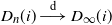 $D_n(i)\overset{\textrm{d}}\longrightarrow D_{\infty}(i)$
. Using the continuous mapping
$D_n(i)\overset{\textrm{d}}\longrightarrow D_{\infty}(i)$
. Using the continuous mapping
 $x\mapsto x(x-1)$
we have, by the continuous mapping theorem, convergence in distribution of the number of wedges
$x\mapsto x(x-1)$
we have, by the continuous mapping theorem, convergence in distribution of the number of wedges
 $\mathbb{W}_n(i)$
:
$\mathbb{W}_n(i)$
:
 \begin{equation*} \mathbb{W}_n(i) = D_n(i)(D_n(i)-1) \overset{\textrm{d}}\longrightarrow D_{\infty}(i)(D_{\infty}(i)-1) \equiv \mathbb{W}_{\infty}(i). \end{equation*}
We then show that the tail satisfies
 $\mathbb{P}(\mathbb{W}_\infty(i) \, {\gt} \, x) \sim \Gamma(1-\alpha)x^{-1/2}$
as
$\mathbb{P}(\mathbb{W}_\infty(i) \, {\gt} \, x) \sim \Gamma(1-\alpha)x^{-1/2}$
as
 $x\to\infty$
by bounding the ratio
$x\to\infty$
by bounding the ratio
 \begin{align*}\frac{\mathbb{P}(D_{\infty}(i)^2 -D_{\infty}(i) \, {\gt} \, x)}{\mathbb{P}(D_{\infty}(i)^2 \, {\gt} \, x)},\end{align*}
where, by (2.4),
 $\mathbb{P}(D_{\infty}(i)^2 \, {\gt} \, x) \sim \Gamma(1-\alpha) x^{-1/2}$
. Let
$\mathbb{P}(D_{\infty}(i)^2 \, {\gt} \, x) \sim \Gamma(1-\alpha) x^{-1/2}$
. Let
 $\delta\, {\gt} \,0$
. Then
$\delta\, {\gt} \,0$
. Then
 \begin{align*} \mathbb{P}(D_{\infty}(i)^2 - D_\infty(i) \, {\gt} \, x) & = \mathbb{P}(D_\infty(i)^2 \, {\gt} \, x + D_\infty(i), D_\infty(i) \, {\gt} \, x + \delta) \\ & \quad + \mathbb{P}(D_{\infty}(i)^2 \, {\gt} \, x + D_{\infty}(i), D_{\infty}(i) \leq x + \delta) \\ & \leq \mathbb{P}(D_{\infty}(i) \, {\gt} \, x+\delta) + \mathbb{P}(D_{\infty}(i)^2\, {\gt} \, x). \end{align*}
This implies that, for any
 $\delta\, {\gt} \,0$
,
$\delta\, {\gt} \,0$
,
 \begin{equation*} \frac{\mathbb{P}(\mathbb{W}_\infty(i)\, {\gt} \,x)}{\mathbb{P}(D_{\infty}(i)^2\, {\gt} \,x)} \leq \frac{\mathbb{P}(D_{\infty}(i) \, {\gt} \, x + \delta)}{\mathbb{P}(D_{\infty}(i)^2 \, {\gt} \, x)} + 1 \sim \frac{\Gamma(1-\alpha)(x + \delta)^{-1}}{\Gamma(1-\alpha)x^{-1/2}} + 1 \xrightarrow[x \to \infty]{} 1. \end{equation*}
A similar break-up yields the lower bound:
 \begin{align*} \mathbb{P}(D_{\infty}(i)^2 - D_{\infty}(i) \, {\gt} \, x) & \geq \mathbb{P}(D_{\infty}(i)^2 \, {\gt} \, (1+\delta)x, D_{\infty}(i) \leq \delta x) \\ & \geq \mathbb{P}(D_{\infty}(i)^2 \, {\gt} \, (1+\delta)x) - \mathbb{P}(D_{\infty}(i) \, {\gt} \, \delta x), \end{align*}
which yields
 \begin{equation*} \frac{\mathbb{P}(D_{\infty}(i)^2 - D_{\infty}(i) \, {\gt} \, x)}{\mathbb{P}(D_{\infty}(i)^2 \, {\gt} \, x)} \geq \frac{((1+\delta)x)^{-1/2} - (\delta x)^{-1}}{x^{-1/2}} \xrightarrow[x\to\infty]{} \frac{1}{\sqrt{1+\delta}\,}. \end{equation*}
Hence,
 \begin{equation*} \limsup_{x\to\infty}\frac{\mathbb{P}(\mathbb{W}_\infty(i)\, {\gt} \,x)}{\Gamma(1-\alpha)x^{-1/2}} \le 1; \qquad \liminf_{x\to\infty}\frac{\mathbb{P}(\mathbb{W}_\infty(i)\, {\gt} \,x)}{\Gamma(1-\alpha)x^{-1/2}} \ge \frac{1}{\sqrt{(1+\delta)}\,}. \end{equation*}
The result follows by taking
 $\delta\to 0$
.
$\delta\to 0$
.
For (iii), we focus on the average number of triangles, whose evaluation will require integral asymptotics similar to those used for the wedges:
 \begin{align*} 6\mathbf{E}[\Delta_n(i)] & = \mathbf{E}\Bigg[\sum_{j \neq i}\sum_{k \neq i,j}a_{ij}a_{ik}a_{jk}\Bigg] \\ & = \sum_{j \neq i}\sum_{k \neq i,j}\mathbb{E}[p_{ij} \, p_{ik} \, p_{jk}] \\ & = (n-1)(n-2)\alpha^3\int_1^{\infty}\int_1^{\infty}\int_1^{\infty} \frac{(1-\textrm{e}^{-\varepsilon xy})(1-\textrm{e}^{-\varepsilon xz})(1-\textrm{e}^{-\varepsilon yz})}{(xyz)^{\alpha+1}}\,\textrm{d} x\,\textrm{d} y\,\textrm{d} z. \end{align*}
First, we provide an upper bound for the above integral. To do this, we use the variables
 $ A = xy $
,
$ A = xy $
,
 $ B = xz $
, and
$ B = xz $
, and
 $ C = yz $
. Note that by setting
$ C = yz $
. Note that by setting
 $ x = \sqrt{{AC}/{B}} $
,
$ x = \sqrt{{AC}/{B}} $
,
 $ y = \sqrt{{AB}/{C}} $
, and
$ y = \sqrt{{AB}/{C}} $
, and
 $ z = \sqrt{{BC}/{A}} $
, and considering that the Jacobian of this transformation is
$ z = \sqrt{{BC}/{A}} $
, and considering that the Jacobian of this transformation is
 $ \frac{1}{4} (ABC)^{-1/2} $
, we have
$ \frac{1}{4} (ABC)^{-1/2} $
, we have
 \begin{align*} & \alpha^3\int_1^{\infty}\int_1^{\infty}\int_1^{\infty} \frac{(1-\textrm{e}^{-\varepsilon xy})(1-\textrm{e}^{-\varepsilon xz})(1-\textrm{e}^{-\varepsilon yz})}{(xyz)^{\alpha+1}}\,\textrm{d} x\,\textrm{d} y\,\textrm{d} z \\ & \qquad = \alpha^3\int_1^{\infty}\int_1^{\infty}\int_{({A}/{B})\vee({B}/{A})}^{AB} \frac{(1-\textrm{e}^{-\varepsilon A})(1-\textrm{e}^{-\varepsilon B})(1-\textrm{e}^{-\varepsilon C})}{(\sqrt{ABC})^{\alpha+1}} \frac{1}{4\sqrt{ABC}\,}\,\textrm{d} C\,\textrm{d} B\,\textrm{d} A \\ & \qquad = \frac{\alpha^3}{4}\int_1^{\infty}\int_1^{\infty}\int_{({A}/{B})\vee({B}/{A})}^{AB} \frac{(1-\textrm{e}^{-\varepsilon A})(1-\textrm{e}^{-\varepsilon B})(1-\textrm{e}^{-\varepsilon C})}{(ABC)^{{\alpha}/{2}+1}}\,\textrm{d} C\,\textrm{d} B\,\textrm{d} A. \end{align*}
Observing that for
 $A, B\ge 1$
the interval
$A, B\ge 1$
the interval
 $(({A}/{B})\vee({B}/{A}),AB)$
is contained in
$(({A}/{B})\vee({B}/{A}),AB)$
is contained in
 $[1,\infty)$
, the last integral can be upper bounded by
$[1,\infty)$
, the last integral can be upper bounded by
 \begin{align*} & \frac{\alpha^3}{4}\int_1^{\infty}\int_1^{\infty}\int_{({A}/{B})\vee({B}/{A})}^{AB} \frac{(1-\textrm{e}^{-\varepsilon A})(1-\textrm{e}^{-\varepsilon B})(1-\textrm{e}^{-\varepsilon C})}{(ABC)^{{\alpha}/{2}+1}}\,\textrm{d} C\,\textrm{d} B\,\textrm{d} A \\ & \qquad \le \frac{\alpha^3}{4}\int_1^{\infty}\int_1^{\infty}\int_1^\infty \frac{(1-\textrm{e}^{-\varepsilon A})(1-\textrm{e}^{-\varepsilon B})(1-\textrm{e}^{-\varepsilon C})}{(ABC)^{{\alpha}/{2}+1}}\,\textrm{d} C\,\textrm{d} B\,\textrm{d} A \\ & \qquad = \frac{\alpha^3}{4}\bigg(\int_1^\infty\frac{1-\textrm{e}^{-\varepsilon A}}{A^{{\alpha}/{2}+1}}\,\textrm{d} A\bigg)^3 \\ & \qquad = \frac{\alpha^3}{4}\bigg[\frac{2}{\alpha} - \varepsilon^{\alpha/2}\Gamma\bigg({-}\frac{\alpha}{2};\varepsilon\bigg)\bigg]^3 \\ & \qquad = \frac{\alpha^3}{4}\bigg[{-}\varepsilon^{\alpha/2}\Gamma\bigg({-}\frac{\alpha}{2}\bigg)+O\!\left(\varepsilon\right)\bigg]^3 = -\frac{n^2\alpha^3}{2}\varepsilon^{{3\alpha}/{2}}\Gamma\bigg({-}\frac{\alpha}{2}\bigg)^3 + O\!\left(n^2\varepsilon^3\right), \end{align*}
where in the last step we used the expansion approximating the incomplete Gamma function (5.2). By our assumption, since
 $\alpha {\, \lt \,} 2$
and
$\alpha {\, \lt \,} 2$
and
 $\varepsilon\to 0$
, we have
$\varepsilon\to 0$
, we have
 $\varepsilon^3=o\!\left(\varepsilon^{{3\alpha}/{2}}\right)$
, and hence
$\varepsilon^3=o\!\left(\varepsilon^{{3\alpha}/{2}}\right)$
, and hence
 $\mathbf{E}[\Delta_n(i)] = O\!\left(n^2\varepsilon^{{3\alpha}/{2}}\right)$
.
$\mathbf{E}[\Delta_n(i)] = O\!\left(n^2\varepsilon^{{3\alpha}/{2}}\right)$
.
To complete the proof, we now show a lower bound that matches the correct order. Specifically, we provide a lower bound for the integral
 \[ I = \int_1^{\infty}\int_1^{\infty}\int_1^{\infty} \frac{(1-\textrm{e}^{-\varepsilon xy})(1-\textrm{e}^{-\varepsilon xz})(1-\textrm{e}^{-\varepsilon yz})}{(xyz)^{\alpha+1}}\,\textrm{d} x\,\textrm{d} y\,\textrm{d} z. \]
First, we perform a change of variables with
 $ x= u/\sqrt{\varepsilon} $
,
$ x= u/\sqrt{\varepsilon} $
,
 $ y= v/\sqrt{\varepsilon} $
, and
$ y= v/\sqrt{\varepsilon} $
, and
 $ z= w/\sqrt{\varepsilon} $
. Then we obtain
$ z= w/\sqrt{\varepsilon} $
. Then we obtain
 \[ I = \varepsilon^{{3\alpha}/{2}}\int_{\sqrt{\varepsilon}}^\infty\int_{\sqrt{\varepsilon}}^\infty\int_{\sqrt{\varepsilon}}^\infty \frac{(1-\textrm{e}^{-uv})(1-\textrm{e}^{-vw})(1-\textrm{e}^{-uw})}{(uvw)^{\alpha+1}}\,\textrm{d} u\,\textrm{d} v\,\textrm{d} w. \]
Since
 $ \varepsilon {\lt} 1 $
, it is not difficult to see that
$ \varepsilon {\lt} 1 $
, it is not difficult to see that
 \[ I \geq \varepsilon^{{3\alpha}/{2}}\int_{1}^\infty\int_{1}^\infty\int_{1}^\infty \frac{(1-\textrm{e}^{-uv})(1-\textrm{e}^{-vw})(1-\textrm{e}^{-uw})}{(uvw)^{\alpha+1}}\,\textrm{d} u\,\textrm{d} v\,\textrm{d} w = c_{\alpha}\varepsilon^{{3\alpha}/{2}}, \]
where
 $ c_{\alpha} \in (0,\infty) $
denotes the value of the above integral. This completes the proof of the lower bound.
$ c_{\alpha} \in (0,\infty) $
denotes the value of the above integral. This completes the proof of the lower bound.
For (iv), let
 $\varepsilon = n^{-1/\alpha}$
; then
$\varepsilon = n^{-1/\alpha}$
; then
 $\mathbb{E}[\Delta_n(i)] \asymp n^{1/2}$
. The above computations also show that
$\mathbb{E}[\Delta_n(i)] \asymp n^{1/2}$
. The above computations also show that
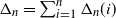 $\Delta_n=\sum_{i=1}^n \Delta_n(i)$
behaves as
$\Delta_n=\sum_{i=1}^n \Delta_n(i)$
behaves as
 \begin{equation} \mathbb{E}[\Delta_n]\asymp n^{3/2}. \end{equation}
To study the concentration of the latter quantity, we start by evaluating the second moment:
 \begin{equation*} \mathbf{E}\big[{\Delta_n^2}\big] = \mathbf{E}\Bigg[\sideset{}{'}\sum_{i,j,k}\sideset{}{'}\sum_{u,v,w}a_{ij}a_{ik}a_{jk}a_{uv}a_{uw}a_{vw}\Bigg] = A + B + C + D, \end{equation*}
where A represents the term in which there is no intersection between the triples of indices of the two summations (
 $(u, v, w) \neq (i, j, k)$
), i.e.
$(u, v, w) \neq (i, j, k)$
), i.e.
 $|\{u, v, w\}\cap \{i,j,k\}|=0$
; B is the term in which there is an intersection of one index, i.e.
$|\{u, v, w\}\cap \{i,j,k\}|=0$
; B is the term in which there is an intersection of one index, i.e.
 $|\{u, v, w\}\cap \{i,j,k\}|=1$
; C is an intersection of two indices, i.e.
$|\{u, v, w\}\cap \{i,j,k\}|=1$
; C is an intersection of two indices, i.e.
 $|\{u, v, w\}\cap \{i,j,k\}|=2$
; and D is the term in which all the indices coincide,
$|\{u, v, w\}\cap \{i,j,k\}|=2$
; and D is the term in which all the indices coincide,
 $|\{u, v, w\}\cap \{i,j,k\}|=3$
.
$|\{u, v, w\}\cap \{i,j,k\}|=3$
.
 $\sum_{i,j,k}^\prime$
means sum over distinct indices.
$\sum_{i,j,k}^\prime$
means sum over distinct indices.
For A, with no common indices,
 \begin{multline*} A = \mathbf{E}\Bigg[\sideset{}{'}\sum_{i,j,k}\sideset{}{'}\sum_{(u,v,w)\neq(i,j,k)} a_{ij}a_{ik}a_{jk}a_{uv}a_{uw}a_{vw}\Bigg] \\ = \mathbf{E}\Bigg[\sideset{}{'}\sum_{i,j,k}a_{ij}a_{ik}a_{jk}\Bigg] \mathbf{E}\Bigg[\sideset{}{'}\sum_{u,v,w}a_{uv}a_{uw}a_{vw}\Bigg] = \mathbf{E}[\Delta_n]^2. \end{multline*}
For B, with one common index,
 \begin{align*} B & = \mathbf{E}\Bigg[\sideset{}{'}\sum_{i,j,k}\sideset{}{'}\sum_\textrm{1 intersection} a_{ij}a_{ik}a_{jk}a_{uv}a_{uw}a_{vw}\Bigg] \\ & = \mathbf{E}\Bigg[\sum_{i,j,k}a_{ij}a_{ik}a_{jk}\,3\sum_{v,w}a_{vw}(a_{iv}a_{iw} + a_{jv}a_{jw} + a_{kv}a_{kw})\Bigg] \\ & \leq \mathbf{E}\Bigg[\sum_{i,j,k}a_{ij}a_{ik}a_{jk}\,9\sum_{v,w}a_{vw}\Bigg] = 9n\mathbf{E}[\Delta_n]\mathbf{E}[D_n(i)]. \end{align*}
For C, with exactly two common indices,
 \begin{equation*} C = \mathbf{E}\Bigg[\sideset{}{'}\sum_{i,j,k}\sideset{}{'}\sum_\textrm{2 intersections} a_{ij}a_{ik}a_{jk}a_{uv}a_{uw}a_{vw}\Bigg] \leq 6n\mathbf{E}\Bigg[\sideset{}{'}\sum_{i,j,k}a_{ij}a_{ik}a_{jk}\Bigg] = 6n\mathbf{E}[\Delta_n]. \end{equation*}
For D, with all indices matching,
 \begin{equation*} D = \mathbf{E}\Bigg[\sideset{}{'}\sum_{i,j,k}a_{ij}a_{ik}a_{jk}a_{ij}a_{ik}a_{jk}\Bigg] = \mathbf{E}\Bigg[\sideset{}{'}\sum_{i,j,k}a_{ij}a_{ik}a_{jk}\Bigg] = \mathbf{E}[\Delta_n]. \end{equation*}
Therefore,
 \begin{align*} \frac{\textrm{Var}(\Delta_n)}{\mathbf{E}[\Delta_n]^2} = \frac{\mathbf{E}[\Delta_n^2] - \mathbf{E}[\Delta_n]^2}{\mathbf{E}[\Delta_n]^2} & = \frac{B+C+D}{\mathbf{E}[\Delta_n]^2} \\[5pt] & \leq \frac{9n\mathbf{E}[\Delta_n]\mathbf{E}[D_n(i)] + 6n\mathbf{E}[\Delta_n] + \mathbf{E}[\Delta_n]} {\mathbf{E}[\Delta_n]^2} \\[5pt] & \le \frac{c_7\big(n^{5/2}\log n + n^{5/2} + n^{3/2}\big)}{c_6n^3} = O\!\left(\frac{\log n}{n^{1/2}}\right), \end{align*}
where
 $c_6$
and
$c_6$
and
 $c_7$
are positive constants, taken respectively from (5.3) and (2.3). Now, using Chebyshev’s inquality it follows that for any
$c_7$
are positive constants, taken respectively from (5.3) and (2.3). Now, using Chebyshev’s inquality it follows that for any
 $\delta\, {\gt} \,0$
,
$\delta\, {\gt} \,0$
,
 \begin{align*} \mathbb{P}\bigg(\bigg|\frac{\Delta_n}{\mathbb{E}[\Delta_n]} - 1\bigg| \ge \delta\bigg) \le \frac{\textrm{Var}(\Delta_n)}{\delta^2\mathbf{E}[\Delta_n]^2} = O\!\left(\frac{\log n}{n^{1/2}}\right). \end{align*}
This completes the proof of the first statement in part (iv). The second one follows from the very same computations.
6. Absence of dust: Proof of Proposition 2.1
We begin with some nice bounds for the incomplete Gamma function.
Lemma 6.1. Let
 $s=(1-\alpha)\in (0,1)$
and let
$s=(1-\alpha)\in (0,1)$
and let
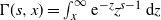 $\Gamma(s, x) = \int_x^\infty\textrm{e}^{-z}z^{s-1}\,\textrm{d} z$
,
$\Gamma(s, x) = \int_x^\infty\textrm{e}^{-z}z^{s-1}\,\textrm{d} z$
,
 $x\, {\gt} \,0$
. Then
$x\, {\gt} \,0$
. Then
 \begin{align*}\textrm{e}^{-x}(1+x)^{s-1} \le \Gamma(s,x) \le \textrm{e}^{-x}\Gamma(s) \bigg(1+\frac{x}{s}\bigg)^{s-1}.\end{align*}
Proof. The proof is a standard use of Jensen’s inequality but we provide the details for completeness. First we show the lower bound. Let
 \begin{align*} \Gamma(s,x) = \int_x^\infty z^{s-1}\textrm{e}^{-z}\,\textrm{d} z = \textrm{e}^{-x}\int_0^\infty(z+x)^{s-1}\textrm{e}^{-z}\,\textrm{d} z = \textrm{e}^{-x}\mathbb{E}[(Z+x)^{s-1}], \end{align*}
where Z is an exponential random variable with parameter 1. Define the function
 $g(t)=(t+x)^{s-1}$
. As
$g(t)=(t+x)^{s-1}$
. As
 $s\in (0,1)$
, g(t) is a convex function. Hence, by Jensen’s inequality we have
$s\in (0,1)$
, g(t) is a convex function. Hence, by Jensen’s inequality we have
 \begin{align*}\Gamma(s,x) = \textrm{e}^{-x}\mathbb{E}[g(Z)] \ge \textrm{e}^{-x}g(\mathbb{E}[Z]) = \textrm{e}^{-x}g(1),\end{align*}
which gives the lower bound. For the upper bound, we again represent the incomplete Gamma function as
 \begin{align*} \Gamma(s,x) = \textrm{e}^{-x}\int_0^{\infty}\bigg(1+\frac{x}{z}\bigg)^{s-1}z^{s-1}\textrm{e}^{-z}\,\textrm{d} z = \textrm{e}^{-x}\Gamma(s)\mathbb{E}\bigg[\bigg(1+\frac{x}{G}\bigg)^{s-1}\bigg], \end{align*}
where G is a Gamma distribution with shape parameter s and rate 1. Using the function
 $h(t)= (1+x/t)^{s-1}$
, which is a concave function, and using the reverse Jensen’s inequality we have
$h(t)= (1+x/t)^{s-1}$
, which is a concave function, and using the reverse Jensen’s inequality we have
 \begin{align*}\Gamma(s,x) = \textrm{e}^{-x}\Gamma(s)\mathbb{E}[h(G)] \le \textrm{e}^{-x}\Gamma(s)h(\mathbb{E}[G]) = \textrm{e}^{-x}\Gamma(s)h(s),\end{align*}
where we used
 $\mathbb{E}[G]=s$
. This gives the upper bound.
$\mathbb{E}[G]=s$
. This gives the upper bound.
The following is a non-standard bound that improves the well-known bound
 $1-\textrm{e}^{-x}\le x$
.
$1-\textrm{e}^{-x}\le x$
.
Lemma 6.2. For
 $\alpha\in [0,1]$
and
$\alpha\in [0,1]$
and
 $x\, {\gt} \,0$
,
$x\, {\gt} \,0$
,
 $1-\textrm{e}^{-x} \le x^{\alpha}$
.
$1-\textrm{e}^{-x} \le x^{\alpha}$
.
Proof. The proof follows by considering the function
 $h(\alpha, x)= 1-\textrm{e}^{-x}-x^{\alpha}$
and studying the derivative with respect to
$h(\alpha, x)= 1-\textrm{e}^{-x}-x^{\alpha}$
and studying the derivative with respect to
 $\alpha$
,
$\alpha$
,
 ${\partial h(\alpha, x)}/{\partial \alpha} = -x^\alpha \ln x$
.
${\partial h(\alpha, x)}/{\partial \alpha} = -x^\alpha \ln x$
.
The next lemma gives a bound on the conditional degree distribution.
Lemma 6.3. For
 $i\in [n]$
,
$i\in [n]$
,
 $j\neq i$
, and
$j\neq i$
, and
 $w\, {\gt} \,1$
,
$w\, {\gt} \,1$
,
 \begin{equation*} \varepsilon^{\alpha}w^{\alpha}\textrm{e}^{-(1+\alpha)\varepsilon w} \le \mathbb{E}[p_{ij} \mid W_i=w] \le \varepsilon^{\alpha}w^\alpha(1+\Gamma(1-\alpha)\textrm{e}^{-\varepsilon w}). \end{equation*}
In particular, for fixed
 $w\, {\gt} \,1$
,
$w\, {\gt} \,1$
,
 \begin{equation} \mathbb{E}[p_{ij} \mid W_i=w] \sim \Gamma(1-\alpha)\varepsilon^{\alpha}w^{\alpha} \quad \text{as $\varepsilon\downarrow 0$}. \end{equation}
Proof.
 \begin{align*} \mathbb{E}[p_{ij} \mid W_i=w] & = \mathbb{E}\big[\big(1-\textrm{e}^{-\varepsilon W_j w}\big)\big] \\ & = \int_0^\infty(1-\textrm{e}^{-\varepsilon wu})\,F_W(\textrm{d} u) = \int_0^\infty\int_0^u\textrm{e}^{-\varepsilon wz}(\varepsilon w)\,\textrm{d} z\,F_W(\textrm{d} u) \\ & = \varepsilon w\int_0^\infty\textrm{e}^{-\varepsilon wz}\mathbb{P}(W_j\, {\gt} \,z)\,\textrm{d} z, \end{align*}
where we used Fubini’s theorem to swap the integrals. Using the fact that the
 $W_j$
are supported on
$W_j$
are supported on
 $(1,\infty)$
we get
$(1,\infty)$
we get
 \begin{align} \mathbb{E}[p_{ij} \mid W_i=w] & = \varepsilon w\int_0^1\textrm{e}^{-\varepsilon wz}\,\textrm{d} z+ \varepsilon w\int_1^\infty\textrm{e}^{-\varepsilon wz}z^{-\alpha}\,\textrm{d} z \nonumber \\ & = (1-\textrm{e}^{-\varepsilon w}) + \varepsilon^\alpha w^\alpha\int_{\varepsilon w}^\infty\textrm{e}^{-z}z^{-\alpha}\,\textrm{d} z = (1-\textrm{e}^{-\varepsilon w}) + \varepsilon^\alpha w^\alpha\Gamma(1-\alpha,\varepsilon w), \end{align}
where
 $\Gamma(1-\alpha,\varepsilon w)$
is an incomplete Gamma function. Now we can use the bounds from Lemmas 6.1 and 6.2. For the upper bound we have
$\Gamma(1-\alpha,\varepsilon w)$
is an incomplete Gamma function. Now we can use the bounds from Lemmas 6.1 and 6.2. For the upper bound we have
 \begin{align*} \mathbb{E}[p_{ij} \mid W_i=w] \le \varepsilon^{\alpha}w^{\alpha} + \varepsilon^\alpha w^\alpha\Gamma(1-\alpha)\textrm{e}^{-\varepsilon w}\bigg(1 + \frac{\varepsilon w}{1-\alpha}\bigg)^{-\alpha}. \end{align*}
Now using the trivial bounds
 $1+{\varepsilon w}/({1-\alpha})\ge 1$
we have
$1+{\varepsilon w}/({1-\alpha})\ge 1$
we have
 \begin{align*}\mathbb{E}[p_{ij} \mid W_i=w] \le \varepsilon^{\alpha}w^{\alpha}(1+\Gamma(1-\alpha)\textrm{e}^{-\varepsilon w}).\end{align*}
For the lower bound, we ignore the first term in (6.2) and use the lower bound in Lemma 6.1. We have
 \begin{equation*} \mathbb{E}[p_{ij} \mid W_i=w] \ge \varepsilon^\alpha w^{\alpha}\Gamma(1-\alpha,\varepsilon w) \ge \varepsilon^{\alpha}w^\alpha\textrm{e}^{-\varepsilon w}(1+\varepsilon w)^{-\alpha} \ge \varepsilon^{\alpha}w^{\alpha}\textrm{e}^{-\varepsilon w}\textrm{e}^{-\alpha \varepsilon w}, \end{equation*}
where we used
 $1+x\le \textrm{e}^x$
for
$1+x\le \textrm{e}^x$
for
 $x\, {\gt} \,0$
, and hence
$x\, {\gt} \,0$
, and hence
 $(1+x)^{-\alpha}\ge \textrm{e}^{-\alpha x}$
. This completes the proof of the lower bound. The asymptotic estimate in (6.1) follows from (6.2).
$(1+x)^{-\alpha}\ge \textrm{e}^{-\alpha x}$
. This completes the proof of the lower bound. The asymptotic estimate in (6.1) follows from (6.2).
Proof of Proposition 2.1 . From the definition of the number of isolated vertices in (2.8), we compute
 \begin{align} \mathbf{E}[N_0] = \sum_{i=1}^n\mathbf{P}(i {\text{ is isolated}}) & = \sum_{i=1}^n\mathbb{E}\Bigg[\prod_{k \neq i}(1-p_{ik})\Bigg] \nonumber \\ & = \sum_{i=1}^n\mathbb{E}\Bigg[\mathbb{E}_{W_i}\Bigg[\prod_{k \neq i}\textrm{e}^{-\varepsilon W_i W_k}\Bigg]\Bigg] \nonumber \\ & = \sum_{i=1}^n\mathbb{E}\Bigg(\prod_{k\neq i}\mathbb{E}_{W_i}\big[\textrm{e}^{-\varepsilon W_i W_k}\big]\Bigg) \nonumber \\ & = n \mathbb{E}\big[\big(\mathbb{E}_{W_1}\big[\textrm{e}^{-\varepsilon W_1 W_2}\big]\big)^{n-1}\big], \end{align}
where we have used the property of the weights being independent and identically distributed.
We can then estimate asymptotically the last expression by means of (6.1) to obtain
 \begin{equation*} \mathbb{E}\big[\big(\mathbb{E}_{W_1}\big[\textrm{e}^{-\varepsilon W_1 W_2}\big]\big)^{n-1}\big] = \mathbb{E}\big[\textrm{e}^{(n-1)\log(1-\mathbb{E}_{W_1}(p_{12}))}\big] \sim \mathbb{E}\big[\textrm{e}^{-(n-1)\Gamma(1-\alpha)\varepsilon^\alpha W_1^{\alpha}}\big]. \end{equation*}
Plugging this estimate into (6.3) we get
 \begin{align*} \mathbb{E}[N_0] \sim n\mathbb{E}\big[\textrm{e}^{-(n-1)\Gamma(1-\alpha)\varepsilon^\alpha W_1^{\alpha}}\big] = \mathbb{E}\bigg[\exp\bigg\{{-}(n-1)\varepsilon^\alpha\bigg(W_1^\alpha-\frac{\log n}{(n-1)\varepsilon^{\alpha}}\bigg)\bigg\}\bigg]. \end{align*}
By the Markov inequality
 $P(N_0\geq 1)\leq \mathbb{E}[N_0]$
, and noticing that the right-hand side goes to zero as n grows, as soon as
$P(N_0\geq 1)\leq \mathbb{E}[N_0]$
, and noticing that the right-hand side goes to zero as n grows, as soon as
 $\varepsilon^{\alpha} \gg ({\log n})/{(n-1)}$
the claim in (2.9) follows.
$\varepsilon^{\alpha} \gg ({\log n})/{(n-1)}$
the claim in (2.9) follows.
Acknowledgements
The authors thank the referees for their valuable comments. We also thank Elena Matteini for spotting a mistake in the previous version of the article.
Funding information
Part of this work started during M. Lalli’s internship in Lorentz Institute of Theoretical Physics in Leiden, which was supported by the ERASMUS+ Grant Agreement no. 2020-1-IT02-KA103-077946/03. L. Avena and R. S. Hazra were supported by NWO Gravitation Grant 024.002.003-NETWORKS. D. Garlaschelli acknowledges support from the Dutch Econophysics Foundation (Stichting Econophysics, Leiden, the Netherlands). His work is also supported by the European Union – NextGenerationEU – National Recovery and Resilience Plan (Piano Nazionale di Ripresa e Resilienza, PNRR), projects ‘SoBigData.it – Strengthening the Italian RI for Social Mining and Big Data Analytics’ – Grant IR0000013 (no. 3264, 28/12/2021) (https://pnrr.sobigdata.it/) and ‘Reconstruction, Resilience and Recovery of Socio-Economic Networks’ RECON-NET EP_FAIR_005 – PE0000013 ‘FAIR’ – PNRR M4C2 Investment 1.3.
Competing interests
There were no competing interests to declare which arose during the preparation or publication process of this article.
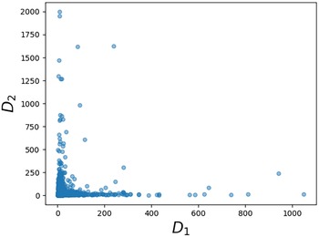


 Open access