



1 Introduction
Extreme values have long been central objects of study in analytic number theory, as they play a crucial role in understanding the Riemann zeta function
$\zeta (s)$
 and Dirichlet L-functions
$L(s,\chi )$
and Dirichlet L-functions
$L(s,\chi )$
 . Such quantities are instrumental in investigating the distribution of values of these functions. In [Reference Soundararajan24], Soundararajan introduced a powerful technique, known as the resonance method, for studying extreme values for various families of
$L(s, \chi )$
. Such quantities are instrumental in investigating the distribution of values of these functions. In [Reference Soundararajan24], Soundararajan introduced a powerful technique, known as the resonance method, for studying extreme values for various families of
$L(s, \chi )$
 . When applied to
$\zeta (s)$
. When applied to
$\zeta (s)$
 , he showed that for sufficiently large T,

Here and throughout, we write
$\log _j$
 for the jth iterated logarithm.
Combining ideas from Aistleitner [Reference Aistleitner1], Bondarenko and Seip [Reference Bondarenko and Seip8, Reference Bondarenko and Seip9] refined Soundararajan’s method and proved that for sufficiently large T,

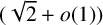
Later, the leading term
$(1+o(1))$
 was improved to
$(\sqrt {2}+o(1))$
was improved to
$(\sqrt {2}+o(1))$
 by de la Bretèche and Tenenbaum [Reference de la Bretèche and Tenenbaum12], by invoking optimized GCD sums.
Recently, Yang [Reference Yang29, Reference Yang31] extended these ideas to derivatives of
$\zeta (s)$
 , obtaining analogous lower bounds in the critical strip. Denote by
$\mathbb {N}$
, obtaining analogous lower bounds in the critical strip. Denote by
$\mathbb {N}$
 the set of all non-negative integers. When
$T \to \infty $
the set of all non-negative integers. When
$T \to \infty $
 , he established the following results concerning GCD sums for
$\ell \in \mathbb {N}$
, he established the following results concerning GCD sums for
$\ell \in \mathbb {N}$
 :
:

and

where
$\sigma \in (1/2, 1)$
 and
$c>0$
and
$c>0$
 is an absolute constant.
Here and throughout this paper, let
$\mathbb {K} = \mathbb {Q}(\omega _d)$
 , where
$\omega _d$
, where
$\omega _d$
 is a dth root of unity for
$d \ge 3$
is a dth root of unity for
$d \ge 3$
 . One of the main motivations for studying the Dedekind zeta function
$\zeta _{\mathbb {K}}(s)$
. One of the main motivations for studying the Dedekind zeta function
$\zeta _{\mathbb {K}}(s)$
 is that it satisfies the following classical factorization:

where the product runs over all non-principal characters
$\chi $
 modulo d, and
$\chi ^{\ast }$
modulo d, and
$\chi ^{\ast }$
 is the character that induces
$\chi $
is the character that induces
$\chi $
 if
$\chi $
if
$\chi $
 is not primitive and
$\chi ^{\ast } = \chi $
is not primitive and
$\chi ^{\ast } = \chi $
 otherwise. Thus, sharper extreme values of
$L(s, \chi )$
otherwise. Thus, sharper extreme values of
$L(s, \chi )$
 may be obtained by studying
$\zeta _{\mathbb {K}}(s)$
may be obtained by studying
$\zeta _{\mathbb {K}}(s)$
 . For a general field
$\mathbb {F}$
. For a general field
$\mathbb {F}$
 , Li [Reference Li22] showed that there exists arbitrarily large t such that

where the magnitude of c depends on whether
$\mathbb {F}/\mathbb {Q}$
 is a Galois extension.
Subsequently, Bondarenko et al. [Reference Bondarenko, Darbar, Hagen, Heap and Seip5] optimized Li’s work and showed that for sufficiently large T,

uniformly for
$d \ll (\log _2T)^A$
 with
$A$
with
$A$
 an arbitrary positive number. Here,
$\phi (n)$
an arbitrary positive number. Here,
$\phi (n)$
 is Euler’s totient function. This conclusion reveals that it is possible to obtain sharper
$\Omega $
is Euler’s totient function. This conclusion reveals that it is possible to obtain sharper
$\Omega $
 -results for
$\zeta (s)$
-results for
$\zeta (s)$
 and
$L(s,\chi )$
and
$L(s,\chi )$
 . Moreover, the best known bound for
$L(s, \chi )$
. Moreover, the best known bound for
$L(s, \chi )$
 ,
,

was established by Soundararajan in [Reference Soundararajan24].
Suppose that
$\mathcal {M} \subset \mathbb {N}$
 is a finite set and let
$\sigma \in (0, 1].$
is a finite set and let
$\sigma \in (0, 1].$
 Define the GCD sums
$S_{\sigma }(\mathcal {M})$
Define the GCD sums
$S_{\sigma }(\mathcal {M})$
 as
as

where
$[m,n]$
 and
$(m,n)$
and
$(m,n)$
 denote the least common multiple and the greatest common divisor of m and n, respectively. Gál [Reference Gál18] derived that
$\sup _{|\mathcal {M}| = N} S_1(\mathcal {M})/|\mathcal {M}| \asymp (\log _2 N)^2$
denote the least common multiple and the greatest common divisor of m and n, respectively. Gál [Reference Gál18] derived that
$\sup _{|\mathcal {M}| = N} S_1(\mathcal {M})/|\mathcal {M}| \asymp (\log _2 N)^2$
 for sufficiently large N. Later, de la Bretèche and Tenenbaum [Reference de la Bretèche and Tenenbaum12] investigated
$S_{1/2}(\mathcal {M})$
for sufficiently large N. Later, de la Bretèche and Tenenbaum [Reference de la Bretèche and Tenenbaum12] investigated
$S_{1/2}(\mathcal {M})$
 and obtained

as
$N \to \infty $
 . For
$1/2 < \sigma < 1,$
. For
$1/2 < \sigma < 1,$
 Aistleitner, Berkes, and Seip [Reference Aistleitner, Berkes and Seip2] proved that

where
$c_{\sigma }$
 and
$C_{\sigma }$
and
$C_{\sigma }$
 are positive constants only depending on
$\sigma $
are positive constants only depending on
$\sigma $
 . They obtained the above bounds by using trigonometric polynomials on the infinite-dimensional polydisc
$\mathbb {D}^{\infty }$
. They obtained the above bounds by using trigonometric polynomials on the infinite-dimensional polydisc
$\mathbb {D}^{\infty }$
 . Notably, their result is almost optimal. GCD sums are powerful tools for studying extreme values of functions related to
$\zeta (s)$
. Notably, their result is almost optimal. GCD sums are powerful tools for studying extreme values of functions related to
$\zeta (s)$
 . Several studies employing GCD sums, including those by Bondarenko and Seip [Reference Bondarenko and Seip8], de la Bretèche and Tenenbaum [Reference de la Bretèche and Tenenbaum12], and Yang [Reference Yang29], have yielded significant results. For more results and details about GCD sums, we recommend [Reference Bondarenko, Hilberdink and Seip6, Reference Bondarenko and Seip7, Reference Lewko and Radziwiłł21] and the references therein.
Motivated by [Reference Bondarenko, Darbar, Hagen, Heap and Seip5, Reference Yang29], we study extreme values of derivatives of
$\zeta _{\mathbb {K}}(s)$
 in the critical strip. We know that

where
$\Re (s)> 1$
 and
$a_{\mathbb {K}}(n)$
and
$a_{\mathbb {K}}(n)$
 is a multiplicative function. Let p be a prime number. By [Reference Washington27], we have

where f denotes the multiplicative order of p in
$(\mathbb {Z}/d\mathbb {Z})^*$
 and
$N(k/f,r)$
and
$N(k/f,r)$
 is the number of ways to write
$k/f$
is the number of ways to write
$k/f$
 as a sum of r non-negative integers.
Henceforth, we assume that
$\ell \in \mathbb {N}$
 . Our main results, Theorems 1.1 and 1.2, establish lower bounds for the maxima of derivatives of
$\zeta _{\mathbb {K}}(s)$
. Our main results, Theorems 1.1 and 1.2, establish lower bounds for the maxima of derivatives of
$\zeta _{\mathbb {K}}(s)$
 both on and near the critical line. Specifically, Theorem 1.1 shows that the lower bound on the critical line attains the same quality as that for
$\zeta _{\mathbb {K}}(s)$
both on and near the critical line. Specifically, Theorem 1.1 shows that the lower bound on the critical line attains the same quality as that for
$\zeta _{\mathbb {K}}(s)$
 itself, while Theorem 1.2 extends the estimate to a suitable range.
Theorem 1.1. Let A be an arbitrary positive number. If T is sufficiently large, then uniformly for
$d \ll (\log _2 T)^A,$


Bondarenko et al. stated in [Reference Bondarenko, Darbar, Hagen, Heap and Seip5] that it is likely that the methods of de la Bretèche and Tenenbaum [Reference de la Bretèche and Tenenbaum12] can improve the exponent on the right-hand side of the above by a factor of
$\sqrt {2}$
 when
$\ell = 0$
when
$\ell = 0$
 . However, since
$a_{\mathbb {K}}(n)$
. However, since
$a_{\mathbb {K}}(n)$
 is not a completely multiplicative function, we have to employ a certain function
$a_{\mathbb {K}}^\prime (n)$
is not a completely multiplicative function, we have to employ a certain function
$a_{\mathbb {K}}^\prime (n)$
 to establish the lower bound for GCD sums. This procedure results in the loss of a factor of
$\sqrt {2}$
to establish the lower bound for GCD sums. This procedure results in the loss of a factor of
$\sqrt {2}$
 . See the Appendix for the details.
Theorem 1.1 refines certain results of [Reference Bondarenko, Darbar, Hagen, Heap and Seip5, Reference Yang29]. In comparison with [Reference Bondarenko, Darbar, Hagen, Heap and Seip5], we derive a lower bound for the maxima of derivatives of
$\zeta _{\mathbb {K}}(s)$
 on the critical line. When
$\ell = 0,$
on the critical line. When
$\ell = 0,$
 it reduces to the case of
$\beta = 0$
it reduces to the case of
$\beta = 0$
 in [Reference Bondarenko, Darbar, Hagen, Heap and Seip5, Theorem 1]. This indicates that the lower bound for the maxima of derivatives of
$\zeta _{\mathbb {K}}(s)$
in [Reference Bondarenko, Darbar, Hagen, Heap and Seip5, Theorem 1]. This indicates that the lower bound for the maxima of derivatives of
$\zeta _{\mathbb {K}}(s)$
 on the critical line can reach the same order as that of the original Dedekind zeta function
$\zeta _{\mathbb {K}}(s)$
on the critical line can reach the same order as that of the original Dedekind zeta function
$\zeta _{\mathbb {K}}(s)$
 . Comparing with [Reference Yang29], we obtain a result that generalizes
$\zeta (s)$
. Comparing with [Reference Yang29], we obtain a result that generalizes
$\zeta (s)$
 . This result corresponds to the case of
$\beta = 0$
. This result corresponds to the case of
$\beta = 0$
 in [Reference Yang29, Theorem 2(A)]. It should be noted that when
$d = 1,2,$
in [Reference Yang29, Theorem 2(A)]. It should be noted that when
$d = 1,2,$
 then
$\mathbb {K}=\mathbb {Q}$
then
$\mathbb {K}=\mathbb {Q}$
 is the rational number field with
$\phi (d)=1$
is the rational number field with
$\phi (d)=1$
 . In this case, Theorem 1.1 is weaker than [Reference Yang29, Theorem 2]. Therefore, we focus on the cases where
$d\ge 3$
. In this case, Theorem 1.1 is weaker than [Reference Yang29, Theorem 2]. Therefore, we focus on the cases where
$d\ge 3$
 , that is, when
$\mathbb {K}$
, that is, when
$\mathbb {K}$
 is not the trivial rational number field
$\mathbb {Q}$
is not the trivial rational number field
$\mathbb {Q}$
 .
.
When the real part
$\sigma $
 is near the critical line, we state the following theorem.
Theorem 1.2. Let A be an arbitrary positive number. Let
$\sigma> 0$
 be a real number and
$T>0$
be a real number and
$T>0$
 sufficiently large in the range

Then, uniformly for
$d \ll (\log _2 T)^A,$


Theorem 1.2 provides a lower bound for the maxima of derivatives of
$\zeta _{\mathbb {K}}(s)$
 near the critical line. Compared with [Reference Bondarenko, Darbar, Hagen, Heap and Seip5, Theorem 1], our leading term in the exponent becomes smaller because the series
$\sum p^{-2\sigma }$
near the critical line. Compared with [Reference Bondarenko, Darbar, Hagen, Heap and Seip5, Theorem 1], our leading term in the exponent becomes smaller because the series
$\sum p^{-2\sigma }$
 can only attain an upper bound similar to [Reference Chirre11, Lemma 9]. We can also apply the same method used in the proof of Theorem 1.2 to study extreme values of derivatives of
$\zeta _{\mathbb {K}}(s)$
can only attain an upper bound similar to [Reference Chirre11, Lemma 9]. We can also apply the same method used in the proof of Theorem 1.2 to study extreme values of derivatives of
$\zeta _{\mathbb {K}}(s)$
 on the critical line, but compared with Theorem 1.1, the leading term in the exponent here is much smaller.
To obtain Theorems 1.1 and 1.2, we rely on the resonance method. This approach was originally proposed by Voronin [Reference Voronin26], although his work did not attract much attention at the time. In 2008, Soundararajan [Reference Soundararajan24] developed the resonance method to study extreme values of
$\zeta (s)$
 and
$L(s, \chi )$
and
$L(s, \chi )$
 . Subsequently, Aistleitner [Reference Aistleitner1] further refined Soundararajan’s resonance method and improved the results of [Reference Hilberdink20, Reference Voronin26]. The resonance method we employ is similar to that refined by Bondarenko and Seip [Reference Bondarenko and Seip8, Reference Bondarenko and Seip9], which follows the ideas of [Reference Aistleitner1] and the slightly modified approach of Chirre [Reference Chirre11]. For more results and details about the resonance method, we recommend [Reference Dong and Wei16, Reference Xu and Yang28, Reference Yang32] and the references therein.
Then, we introduce some notation. Let A be an arbitrarily large positive number and
$\varepsilon $
 be small. We note that each occurrence of A and
$\varepsilon $
be small. We note that each occurrence of A and
$\varepsilon $
 may represent different values. Let
$\mathbb {R}$
may represent different values. Let
$\mathbb {R}$
 denote the set of all real numbers. Finally, we denote the Fourier transform of a function
$f \in L^1(\mathbb {R})$
denote the set of all real numbers. Finally, we denote the Fourier transform of a function
$f \in L^1(\mathbb {R})$
 as
as

Following the argument of Yang [Reference Yang29, p. 4], we define

According to the above definition, it can be written as the following Dirichlet series for
$\Re (s)> 1$
 :
:

which is absolutely convergent. Clearly,
$a(1)=1, a(2) = a_{\mathbb {K}}(2)+a_{\mathbb {K}}(2) (\log 2)^{\ell },$
 and for
$n \ge 3,a(n)=a_{\mathbb {K}}(n)(\log n)^{\ell }.$
and for
$n \ge 3,a(n)=a_{\mathbb {K}}(n)(\log n)^{\ell }.$
 The term
$1 + a_{\mathbb {K}}(2) 2^{-s}$
The term
$1 + a_{\mathbb {K}}(2) 2^{-s}$
 added in the above definition ensures that the inequality
$a(n) \ge a_{\mathbb {K}}(n)$
added in the above definition ensures that the inequality
$a(n) \ge a_{\mathbb {K}}(n)$
 holds for all
$n \ge 1$
holds for all
$n \ge 1$
 . Moreover, we have the trivial upper bound

We now outline the structure of this paper. Section 2 presents several auxiliary lemmas that are used throughout the proofs. In Section 3, we construct an appropriate resonator and prove Theorem 1.1. The proof of Theorem 1.2 is given in Section 4, which is preceded by the construction of another resonator. In Section 5, we present additional results that further refine our study of extreme values of derivatives of
$\zeta _{\mathbb {K}}(s)$
 within the critical strip.
2 Preliminary lemmas
In this section, we present several lemmas for later use. The first lemma provides a growth estimate for derivatives of
$\zeta _{\mathbb {K}}(s)$
 in the critical strip.
Lemma 2.1. Fix
$\delta \in (0, 1/2]$
 . Then, uniformly for all
$|t| \ge 1$
. Then, uniformly for all
$|t| \ge 1$
 and
$-\delta \le \sigma \le 1+\delta $
and
$-\delta \le \sigma \le 1+\delta $
 ,
,

Proof. This estimate follows directly from [Reference Rademacher23, Theorem 4] together with Cauchy’s integral formula.
Remark. A sharper bound for derivatives of
$\zeta _{\mathbb {K}}(s)$
 on the critical line was given in [Reference Heath-Brown19]. According to the Phragmén–Lindelöf theorem, the exponent can be optimized. However, Lemma 2.1 is already sufficient for our purpose.
Furthermore, to establish a connection with GCD sums, we need to use a double-version convolution formula, following the approach of de la Bretèche and Tenenbaum [Reference de la Bretèche and Tenenbaum12, Lemma 5.3]. It is similar to that in [Reference Yang29, Lemma 3]. For the sake of completeness, we provide a proof.
Lemma 2.2. Suppose
$\sigma \in [1/2, 1)$
 and let
$s = x + iy$
and let
$s = x + iy$
 . Let
$K(s)$
. Let
$K(s)$
 be holomorphic in the horizontal strip
$\sigma -2 \le y \le 0,$
be holomorphic in the horizontal strip
$\sigma -2 \le y \le 0,$
 satisfying the growth condition

Then, for all
$t \neq 0,$


where
$\tau ^{+}$
 and
$\tau ^{-}$
and
$\tau ^{-}$
 are given by

Proof. Let
$g(s) {:=}q \mathcal {G}(s + it )\mathcal {G}(s - it)K(i\sigma - is)$
 . The only poles in
$\sigma \le {\textrm {Re}}(s) \le 2$
. The only poles in
$\sigma \le {\textrm {Re}}(s) \le 2$
 occur at
$1 \pm it$
occur at
$1 \pm it$
 .
.
Integrating
$g(s)$
 along the rectangle with vertices
$\sigma \pm iY$
along the rectangle with vertices
$\sigma \pm iY$
 and
$2 \pm iY$
and
$2 \pm iY$
 , and applying the residue theorem, yields

where
$I_1$
 and
$I_3$
and
$I_3$
 are the integrals of
$g(s)$
are the integrals of
$g(s)$
 from
$\sigma - iY$
from
$\sigma - iY$
 to
$2 - iY$
to
$2 - iY$
 and from
$2 + iY$
and from
$2 + iY$
 to
$\sigma + iY$
to
$\sigma + iY$
 , respectively, along the horizontal edges of the rectangle. Meanwhile,
$I_2$
, respectively, along the horizontal edges of the rectangle. Meanwhile,
$I_2$
 and
$I_4$
and
$I_4$
 are the integrals of
$g(s)$
are the integrals of
$g(s)$
 from
$2 - iY$
from
$2 - iY$
 to
$2 + iY$
to
$2 + iY$
 and from
$\sigma + iY$
and from
$\sigma + iY$
 to
$\sigma - iY$
to
$\sigma - iY$
 , respectively, corresponding to the vertical direction. We estimate these four integrals one by one in the subsequent calculations.
It is clear that

the infinite integral on the right-hand side is absolutely convergent due to the rapid decay of K. Moreover, by Cauchy’s theorem, we conclude that

Applying (1-2), Lemma 2.1, and the rapid decay of K, we find that both
$I_1$
 and
$I_3$
and
$I_3$
 are bounded by

Setting
$\delta = 1/12$
 ensures that both
$I_1$
ensures that both
$I_1$
 and
$I_3$
and
$I_3$
 tend to
$0$
tend to
$0$
 as
$Y \to \infty $
as
$Y \to \infty $
 . Substituting this into (2-1) completes the proof.
Similarly, we have the following single-version convolution formula.
Lemma 2.3. Suppose
$\sigma \in [1/2, 1)$
 and let
$s = x + iy$
and let
$s = x + iy$
 . Let
$K(s)$
. Let
$K(s)$
 be holomorphic in the horizontal strip
$\sigma -2 \le y \le 0$
be holomorphic in the horizontal strip
$\sigma -2 \le y \le 0$
 , satisfying the growth condition

Then, for all
$t \neq 0,$


where
$\tau $
 is given by

Proof. Consider
$g_1(s) {:=}q \mathcal {G}(s+it)K(i\sigma -is)$
 . The proof follows similarly to that of Lemma 2.2. Therefore, the details are omitted for brevity.
We need an appropriate smooth kernel function K when applying Lemmas 2.2 and 2.3. Following the ideas in [Reference Bondarenko, Darbar, Hagen, Heap and Seip5, Reference Bondarenko and Seip9], we set

which is the same choice as in [Reference Bondarenko, Darbar, Hagen, Heap and Seip5]. Here,
$\varepsilon $
 is small and
$\eta \in \mathbb {N}$
is small and
$\eta \in \mathbb {N}$
 is chosen later. We present some properties of
$\widehat {K_\eta }$
is chosen later. We present some properties of
$\widehat {K_\eta }$
 , which are used frequently in the subsequent proof.
Lemma 2.4 [Reference Bondarenko, Darbar, Hagen, Heap and Seip5, Lemma 5]
Let
$K_{\eta }(u)$
 be defined as in (2-2). Then,
$\widehat {K_{\eta }}(v)$
be defined as in (2-2). Then,
$\widehat {K_{\eta }}(v)$
 is a real and even function supported on
$|v|\le 2\varepsilon \log T.$
is a real and even function supported on
$|v|\le 2\varepsilon \log T.$
 It is decreasing on
$[0,\infty )$
It is decreasing on
$[0,\infty )$
 and satisfies
$0\le \widehat {K_{\eta }}(v)\le \widehat {K_{\eta }}(0)$
and satisfies
$0\le \widehat {K_{\eta }}(v)\le \widehat {K_{\eta }}(0)$
 . Moreover,

Furthermore, for large
$\eta $
 , the following equivalence holds:

3 Proof of Theorem 1.1
In this section, we apply the auxiliary lemmas from Section 2 to complete the proof of Theorem 1.1. We first establish lower bounds for GCD sums weighted by the coefficients
$a_{\mathbb {K}}(n)$
 .
.
3.1 Lower bounds for weighted GCD sums
We extend the construction introduced by de la Bretèche and Tenenbaum [Reference de la Bretèche and Tenenbaum12]. Define

Let
$\alpha \in (1,e)$
 and
$\delta \in (0,1)$
and
$\delta \in (0,1)$
 be some parameters, and let
$N = \lfloor T^{\lambda } \rfloor $
be some parameters, and let
$N = \lfloor T^{\lambda } \rfloor $
 be an integer not larger than T with
$\lambda $
be an integer not larger than T with
$\lambda $
 to be chosen later. Let k be an integer satisfying
$1\le k \le (\log _{2}N)^{\delta },$
to be chosen later. Let k be an integer satisfying
$1\le k \le (\log _{2}N)^{\delta },$
 then define
$P_k$
then define
$P_k$
 as the set of primes p that satisfy

Since
$d \ll (\log _2 T)^A $
 , the Siegel–Walfisz theorem implies

Let
$\beta> 1$
 satisfy
$\beta \delta \log \alpha < 1$
satisfy
$\beta \delta \log \alpha < 1$
 . We then define

Furthermore, we let
$W {:=}q \prod _{p\in P_{k}}p$
 and consider the following set:

where
$\omega (n)$
 denotes the number of distinct prime factors of n. Next, we consider

According to [Reference de la Bretèche and Tenenbaum12, Lemma 2.2], we have
$|\mathcal {M}|\le N$
 . We establish the following lower bound for
$S_{1/2}(\mathcal {M},a_{\mathbb {K}})$
. We establish the following lower bound for
$S_{1/2}(\mathcal {M},a_{\mathbb {K}})$
 .
.
Proposition 3.1. Define
$S_{1/2}(\mathcal {M},a_{\mathbb {K}})$
 as in (3-1), where
$\mathcal {M}$
as in (3-1), where
$\mathcal {M}$
 is given in (3-2). Then, for
$d \ll (\log _2 T)^A$
is given in (3-2). Then, for
$d \ll (\log _2 T)^A$
 ,
,

as
$N \to \infty $
 .
.
Fonga attempted to extend the results of de la Bretèche and Tenenbaum in [Reference Fonga17, Theorem 1.1]. We argue that the range of k he chose is inappropriate. Even so, the proof of this proposition still follows the idea of Fonga; see [Reference Fonga17, pp. 3–7]. Specifically, note that
$a_{\mathbb {K}}(n)$
 is not a completely multiplicative function. To establish a lower bound for
$S_{1/2}(\mathcal {M},a_{\mathbb {K}})$
is not a completely multiplicative function. To establish a lower bound for
$S_{1/2}(\mathcal {M},a_{\mathbb {K}})$
 , we need to use an auxiliary function
$a_{\mathbb {K}}^\prime (n)$
, we need to use an auxiliary function
$a_{\mathbb {K}}^\prime (n)$
 . For the sake of completeness, we include the proof of Proposition 3.1 in the Appendix.
Remark. For
$1/2 < \sigma <1$
 , one can define analogously

If a lower bound similar to that in Proposition 3.1 can be obtained for
$S_{\sigma }(\mathcal {M},a_{\mathbb {K}})$
 , the result of Theorem 1.2 can be optimized through a process nearly analogous to that of Theorem 1.1.
3.2 Constructing the resonator
Following the ideas from [Reference Bondarenko and Seip8, Reference de la Bretèche and Tenenbaum12, Reference Yang29], we construct the resonator
$R(t)$
 needed to apply the resonance method. For each integer
$j \ge 0$
needed to apply the resonance method. For each integer
$j \ge 0$
 , define

Here, T is a parameter and
$\mathcal {M}$
 is defined as (3-2). Using the notation in [Reference de la Bretèche and Tenenbaum12], we let
$h_j {:=}q \min \mathcal {N}_j$
is defined as (3-2). Using the notation in [Reference de la Bretèche and Tenenbaum12], we let
$h_j {:=}q \min \mathcal {N}_j$
 if
$\mathcal {N}_j \neq \emptyset $
if
$\mathcal {N}_j \neq \emptyset $
 . Define
$\mathcal {H}$
. Define
$\mathcal {H}$
 as the set of all
$h_j$
as the set of all
$h_j$
 and consider the function r on
$\mathcal {H}$
and consider the function r on
$\mathcal {H}$
 defined by

We then define the resonator as follows:

By the Cauchy–Schwarz inequality,

Set
$\Phi (y){:=}q e^{-y^{2}/2}$
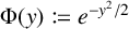 as in [Reference Bondarenko and Seip8]. Plainly, the Fourier transform
$\widehat {\Phi }$
as in [Reference Bondarenko and Seip8]. Plainly, the Fourier transform
$\widehat {\Phi }$
 satisfies
$\widehat {\Phi }(\xi )=\sqrt {2\pi }\Phi (\xi )$
satisfies
$\widehat {\Phi }(\xi )=\sqrt {2\pi }\Phi (\xi )$
 . According to [Reference Bondarenko and Seip9, Lemma 5],

3.3 The proof of Theorem 1.1
We now complete the proof of Theorem 1.1. Let
$\eta = 2\phi (d)$
 as in [Reference Bondarenko, Darbar, Hagen, Heap and Seip5] and
$N = \lfloor T^\lambda \rfloor $
as in [Reference Bondarenko, Darbar, Hagen, Heap and Seip5] and
$N = \lfloor T^\lambda \rfloor $
 . For fixed
$\varepsilon>0$
. For fixed
$\varepsilon>0$
 , we choose
$\lambda $
, we choose
$\lambda $
 such that
$\lambda +5\varepsilon <1$
such that
$\lambda +5\varepsilon <1$
 . We start with the following integral:

We divide
$J(T)$
 into three parts as follows:

For brevity, the integrands on the right-hand side are omitted, without causing any ambiguity. We show that the integral
$J_1(T)$
 provides the main term for
$J(T)$
provides the main term for
$J(T)$
 .
.
Using Lemma 2.1, we establish the following bound:

Combining with
$K_{\eta }(u) \ll u^{-4\phi (d)},$
 it is clear that

Then, by (3-4) and
$d \ll (\log _2 T)^A,$


Moreover,

The rapid decay of
$\Phi $
 and (3-6) implies that

Substituting (3-7), (3-8) into (3-5),

Define

Combining this with (3-4), we immediately derive the following lower bound:

Thus,

Next, we seek an effective lower bound for
$J(T)$
 . Our approach establishes a connection between
$J(T)$
. Our approach establishes a connection between
$J(T)$
 and GCD sums via the double-version convolution formula. We introduce the following three integrals:

where the series
$E(t)$
 is defined as

Lemma 2.2 implies that
$J(T)=J_0(T)+\mathcal {E}^+ +\mathcal {E}^-.$
 As in [Reference Yang30, pp. 14–15],

Subsequently, we use the Fourier transform on the real axis and, therefore, focus on the region
$|t| \le 1$
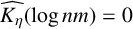
 now. Lemma 2.4 shows that
$\widehat {K_{\eta }}(\log nm)=0$
now. Lemma 2.4 shows that
$\widehat {K_{\eta }}(\log nm)=0$
 when
$mn\ge T^{2\varepsilon }$
when
$mn\ge T^{2\varepsilon }$
 . Thus,

Since
$d \ll (\log _2 T)^A,$
 we have
$a(n)n^{-1/2}\ll (\log _2 T)^A.$
we have
$a(n)n^{-1/2}\ll (\log _2 T)^A.$
 Thus, the integral on
$|t| \le 1$
Thus, the integral on
$|t| \le 1$
 can be bounded by

We extend the integral to
$\mathbb {R}$
 . Specifically, setting

we have

Hence, combining with (3-9),

We now derive the lower bound for
$\widetilde {J}(T)$
 . Expanding
$|R(t)|^2$
. Expanding
$|R(t)|^2$
 and
$E(t)$
and
$E(t)$
 in
$\widetilde {J}(T)$
in
$\widetilde {J}(T)$
 yields that

For the terms involving
$\widehat {K_{\eta }}(u)$
 , we follow the approach in [Reference Bondarenko, Darbar, Hagen, Heap and Seip5, p. 10], using (2-3) and (2-4). For the inner sum, it follows from the proof of [Reference de la Bretèche and Tenenbaum12, Theorem 1.4] that

Setting

we have

Using Rankin’s trick, we can establish a connection between
$\widetilde {J}$
 and weighted GCD sums as follows:

where
$S_{1/2}(\mathcal {M},a_{\mathbb {K}})$
 and
$S_{1/3}(\mathcal {M},a_{\mathbb {K}})$
and
$S_{1/3}(\mathcal {M},a_{\mathbb {K}})$
 are given by (3-1) and (3-3), respectively.
Combining with (3-10),

Following the idea from [Reference de la Bretèche and Tenenbaum12], if we set
$P^+ (m)$
 as the largest prime factor of m and
$y_{\mathcal {M}} {:=}q \max _{m \in \mathcal {M}} P^+(m),$
as the largest prime factor of m and
$y_{\mathcal {M}} {:=}q \max _{m \in \mathcal {M}} P^+(m),$
 then,
then,

Based on the construction of
$P_k$
 in Section 2, we have
$y_{\mathcal {M}} \ll (\log T)^{6/5}$
in Section 2, we have
$y_{\mathcal {M}} \ll (\log T)^{6/5}$
 , so that for sufficiently large T,

Thus, by Proposition 3.1, for all sufficiently large T,

Trivially,

We let
$\lambda $
 be sufficiently close to 1 such that
$\lambda + 5\varepsilon <1$
be sufficiently close to 1 such that
$\lambda + 5\varepsilon <1$
 for small
$\varepsilon $
for small
$\varepsilon $
 . Finally, we set

and readjust the parameter
$T=T^{\prime }$
 following the idea from [Reference Bondarenko, Darbar, Hagen, Heap and Seip5]. Variations in the logarithmic factor affect only the lower order terms in the exponent on the right-hand side of (3-11). Hence, this result also holds for
$t \in [0,T]$
following the idea from [Reference Bondarenko, Darbar, Hagen, Heap and Seip5]. Variations in the logarithmic factor affect only the lower order terms in the exponent on the right-hand side of (3-11). Hence, this result also holds for
$t \in [0,T]$
 . We complete the proof of Theorem 1.1.
4 Proof of Theorem 1.2
In this section, we prove Theorem 1.2 using the resonance method. As in Section 3, we set
$\eta = 2 \phi (d)$
 .
.
4.1 Constructing the resonator
We construct the resonator
$R(t)$
 following a similar strategy as in [Reference Chirre11]. Let
$\gamma \in (0,1)$
following a similar strategy as in [Reference Chirre11]. Let
$\gamma \in (0,1)$
 be a parameter to be chosen later. Define
$\mathcal {P}_d$
be a parameter to be chosen later. Define
$\mathcal {P}_d$
 as the set of prime numbers p such that

For any
$1 \le c_d \le \sqrt {\phi (d)/(e-1)}$
 , define the multiplicative function
$f(n)$
, define the multiplicative function
$f(n)$
 supported on the set of square-free numbers by setting

as
$p \in \mathcal {P}_d$
 , and
$f(p) = 0$
, and
$f(p) = 0$
 otherwise.
For each integer
$k \in \{1, \ldots , \lfloor (\log _2 N)^{\gamma }\rfloor \}$
 , define
$\mathcal {P}_{k,d}$
, define
$\mathcal {P}_{k,d}$
 as the set of p satisfying

which is the subset of
$\mathcal {P}_d$
 . Fixing
$1 < \alpha < 1/\gamma $
. Fixing
$1 < \alpha < 1/\gamma $
 , define

Let
$\mathcal {M}^{\prime }_{k,d}$
 consist of those integers
$\mathcal {M}_{k,d}$
consist of those integers
$\mathcal {M}_{k,d}$
 whose prime factors all lie in
$\mathcal {P}_{k,d}$
whose prime factors all lie in
$\mathcal {P}_{k,d}$
 . Subsequently, set

From the above definitions, we can deduce several useful properties. First,
$\mathcal {M}_d$
 is divisor closed. Specifically, if some
$m^{\prime } \mid m \in \mathcal {M}_d,$
is divisor closed. Specifically, if some
$m^{\prime } \mid m \in \mathcal {M}_d,$
 then
$m^{\prime } \in \mathcal {M}_d$
then
$m^{\prime } \in \mathcal {M}_d$
 . Adapting the argument of [Reference Chirre11, Lemma 8], we obtain that
$|\mathcal {M}_d| \le N$
. Adapting the argument of [Reference Chirre11, Lemma 8], we obtain that
$|\mathcal {M}_d| \le N$
 . Furthermore, the Siegel–Walfisz theorem gives

Now, we construct the resonator
$R(t)$
 . Define
$\mathcal {J}$
. Define
$\mathcal {J}$
 as the set of integers j such that

and let
$m_j$
 be the minimum of
$[(1 + \log T/T)^j, (1 + \log T/T)^{j + 1}] \cap \mathcal {M}_d $
be the minimum of
$[(1 + \log T/T)^j, (1 + \log T/T)^{j + 1}] \cap \mathcal {M}_d $
 for all
$j \in \mathcal {J}.$
for all
$j \in \mathcal {J}.$
 Setting
$\mathcal {M}^{\prime }_d = \{m_j : j \in \mathcal {J} \}$
Setting
$\mathcal {M}^{\prime }_d = \{m_j : j \in \mathcal {J} \}$
 , define

Finally, define

By the Cauchy–Schwarz inequality,

Moreover, taking
$\Phi $
 to be the same as in Section 3 and using [Reference Bondarenko and Seip9, Lemma 5],

4.2 Supporting propositions
Define

Here,
$a_{\mathbb {K}}(n)$
 are the coefficients of the Dirichlet series of
$\zeta _{\mathbb {K}}(s)$
are the coefficients of the Dirichlet series of
$\zeta _{\mathbb {K}}(s)$
 and f is the multiplicative function introduced in Section 4.1. In this subsection, we present some auxiliary propositions that provide a sharp lower bound for
$\mathcal {A}_d$
and f is the multiplicative function introduced in Section 4.1. In this subsection, we present some auxiliary propositions that provide a sharp lower bound for
$\mathcal {A}_d$
 and show that the error terms caused by truncation or the exclusion of
$\mathcal {M}_d$
and show that the error terms caused by truncation or the exclusion of
$\mathcal {M}_d$
 are negligible. These results play a central role in establishing the lower bound in Theorem 1.2.
Proposition 4.1. Let
$d \ll (\log _2 N)^A$
 and
$c_d \le \sqrt {\phi (d)/(e-1)}$
and
$c_d \le \sqrt {\phi (d)/(e-1)}$
 . Then, for
$0 < \delta <1$
. Then, for
$0 < \delta <1$
 as
$N \to +\infty $
as
$N \to +\infty $
 ,
,

Proof. For
$c_d \le \sqrt {\phi (d)/(e-1)}$
 , we have
$f(p)=o(1)$
, we have
$f(p)=o(1)$
 for all
$p \in \mathcal {P}_d$
for all
$p \in \mathcal {P}_d$
 . It follows that

By the definition of
$f(p)$
 ,
,

Notice that from [Reference Chirre11, Lemma 9], we get the following lower bound:

where
$0< \delta <1$
 . Thus,

This completes the proof.
Proposition 4.2. Let
$d \ll (\log _2 N)^A$
 and
$c_d \le \sqrt {\phi (d)/(e-1)}$
and
$c_d \le \sqrt {\phi (d)/(e-1)}$
 . Then, as
$N \to +\infty $
. Then, as
$N \to +\infty $
 ,
,

Proof. By the definition of
$\mathcal {M}_d,$


From the construction of
$f(n)$
 and
$\mathcal {M}_{k,d}^{\prime }$
and
$\mathcal {M}_{k,d}^{\prime }$
 , it follows that
$\mathcal {F}$
, it follows that
$\mathcal {F}$
 can be bounded by

It is clear from (4-1) that

Therefore, combining this with the fact that
$d \ll ( \log _2 N)^A$
 and
$k \le (\log _2 N)^{\gamma }$
and
$k \le (\log _2 N)^{\gamma }$
 ,
,

However, recalling the definition of
$\mathcal {M}^{\prime }_{k,d},$
 we use the classical method in [Reference Bondarenko and Seip8, p. 8]. Since
$f(n)$
we use the classical method in [Reference Bondarenko and Seip8, p. 8]. Since
$f(n)$
 is multiplicative,

whenever
$b>1$
 . Thus,

For the sum in the exponent, the Siegel–Walfisz theorem yields

Combining all the above estimates,
$\mathcal {F}^\star $
 is bounded by

Since
$c_d \le \sqrt {\phi (d)/(e-1)}$
 and
$\alpha>1$
and
$\alpha>1$
 , it suffices to choose b sufficiently close to
$1$
, it suffices to choose b sufficiently close to
$1$
 so that the exponent becomes negative. Hence, the proof is complete.
Proposition 4.3. Let
$d \ll (\log _2 N)^A$
 and
$c_d \le \sqrt {\phi (d)/(e-1)}$
and
$c_d \le \sqrt {\phi (d)/(e-1)}$
 . Then, as
$N \to +\infty $
. Then, as
$N \to +\infty $
 ,
,

Proof. We have

Furthermore, applying Rankin’s trick to the inner sum on the right-hand side yields

Since
$\eta = 2\phi (d)$
 and because each n in
$\mathcal {M}_d$
and because each n in
$\mathcal {M}_d$
 has at most
$ O((\log N / \log _3 N)^{2-2\sigma })$
has at most
$ O((\log N / \log _3 N)^{2-2\sigma })$
 prime factors, the proof follows by a process similar to that in [Reference Bondarenko, Darbar, Hagen, Heap and Seip5, Lemma 6].
4.3 The proof of Theorem 1.2
In this subsection, the ideas and techniques in our preceding part are essentially the same as those used in Section 3.3. Let
$N=\lfloor T^\lambda \rfloor $
 , where
$\lambda + 2 \varepsilon < 1$
, where
$\lambda + 2 \varepsilon < 1$
 holds for small
$\varepsilon $
holds for small
$\varepsilon $
 . Define

and

Trivially,

Then, we proceed by considering the tails of the integrals:

The following upper bound for
$W_2(T)$
 can be established by using Lemma 2.1 and the fact that
$K_{\eta }(u) \ll u^{-4\phi (d)}$
can be established by using Lemma 2.1 and the fact that
$K_{\eta }(u) \ll u^{-4\phi (d)}$
 ,
,

Furthermore, for
$W_3(T)$
 , applying Lemma 2.1,

Since
$\Phi $
 decays rapidly,

Equations (4-2) and (4-3) yield the following result:

where

Then, define

Cauchy’s integral formula implies
$\mathcal {E} = o(T^{\lambda } \sum _{n \in \mathbb {N}}f(n)^2)$
 , and thus,

To extend the t integral to
$\mathbb {R}$
 , we consider the integral over the region
$|t| \le 1$
, we consider the integral over the region
$|t| \le 1$
 . Plainly,

Combining this with Lemma 2.4, we deduce that

Recalling that
$\lambda + 2\varepsilon <1$
 and combining (4-4), (4-5), and (4-6), it follows that

Denoting
$\widetilde {W}(T)$
 as the integral on the right-hand side of the preceding inequality,

Here, we note the fact that
$a(n) \ge a_{\mathbb {K}}(n)$
 . Following the idea of [Reference Bondarenko, Darbar, Hagen, Heap and Seip5], we restrict the inner sum to
$k \le T^{\varepsilon /3\eta }$
. Following the idea of [Reference Bondarenko, Darbar, Hagen, Heap and Seip5], we restrict the inner sum to
$k \le T^{\varepsilon /3\eta }$
 , yielding

Employing techniques similar to those in [Reference Bondarenko and Seip9, (21)],

Combining Propositions 4.1, 4.2, and 4.3 yields

for
$\lambda + 2\varepsilon <1.$
 Then,
Then,

Let
$\lambda +2 \varepsilon <1$
 with small
$\varepsilon $
with small
$\varepsilon $
 . By choosing
$\delta $
. By choosing
$\delta $
 ,
$\gamma $
,
$\gamma $
 , and
$c_d$
, and
$c_d$
 to be sufficiently close respectively to
$1$
to be sufficiently close respectively to
$1$
 ,
$1$
,
$1$
 , and
$\sqrt {\phi (d)/(e-1)}$
, and
$\sqrt {\phi (d)/(e-1)}$
 , and applying the same transform as in Section 3.3, we conclude the proof of Theorem 1.2.
5 Supplementary conclusions
In Sections 3 and 4, we present Theorems 1.1 and 1.2 along with their proofs. These theorems establish lower bounds for the maxima of derivatives of
$\zeta _{\mathbb {K}}(s)$
 on and near the critical line.
Inspired by [Reference Dong, Song, Wang and Zhang15], we present the following conclusion. Since the method used is almost identical to that in Section 4, we omit the proof here and recommend [Reference Dong, Li, Song and Zhao14] for further details.
Theorem 5.1. Let A and D be arbitrary positive numbers, and T be sufficiently large. Set
$\sigma _D {:=}q 1/2 + D/(\log _2 T)$
 . Then, uniformly for
$d \ll (\log _2T)^A,$
. Then, uniformly for
$d \ll (\log _2T)^A,$


Unfortunately, the set
$\mathcal {M}_d$
 and the resonator
$R(t)$
and the resonator
$R(t)$
 constructed in Section 4.1 can only be used to study extreme values within the region where
$|\sigma -1/2| \ll (\log _2T)^{-1}$
constructed in Section 4.1 can only be used to study extreme values within the region where
$|\sigma -1/2| \ll (\log _2T)^{-1}$
 . For the larger range beyond this, we supplement with the following result.
Theorem 5.2. Let A be an arbitrary positive number. If T is sufficiently large in the range
$1/2 \le \sigma \le 2/3$
 , then uniformly for
$d \ll (\log _2T)^A,$
, then uniformly for
$d \ll (\log _2T)^A,$


Proof. In fact, we only need to redefine the set
$\mathcal {M}_{k,d}$
 as
as

and the value of
$f(p)$
 for
$p \in \mathcal {P}_d$
for
$p \in \mathcal {P}_d$
 as
as

Here, the definitions of
$\mathcal {P}_d$
 and
$\mathcal {P}_{k,d}$
and
$\mathcal {P}_{k,d}$
 remain unchanged, and the remainder of the argument proceeds as in Section 4.3.
It is worth noting that using a similar method as in [Reference Bondarenko and Seip10], we can extend the above result almost to the region
$1/2 < \sigma < \sigma _0$
 for any fixed
$\sigma _0$
for any fixed
$\sigma _0$
 such that
$1/2<\sigma _0<1$
such that
$1/2<\sigma _0<1$
 ,
,

The constant
$C(\sigma )$
 depends on
$\sigma $
depends on
$\sigma $
 . Thus, in the critical strip, derivatives of
$\zeta _{\mathbb {K}}(s)$
. Thus, in the critical strip, derivatives of
$\zeta _{\mathbb {K}}(s)$
 attain extreme values of the same order of magnitude as those in [Reference Yang29, Theorem 2(B)] for
$\zeta (s)$
attain extreme values of the same order of magnitude as those in [Reference Yang29, Theorem 2(B)] for
$\zeta (s)$
 .
.
When
$\sigma =1$
 , Dixit and Mahatab [Reference Dixit and Mahatab13] used the long resonator method to obtain extreme values of the Dedekind zeta function of a general number field
$\mathbb {F}$
, Dixit and Mahatab [Reference Dixit and Mahatab13] used the long resonator method to obtain extreme values of the Dedekind zeta function of a general number field
$\mathbb {F}$
 . More precisely, for sufficiently large T, there exists a positive constant
$C_{\mathbb {F}}$
. More precisely, for sufficiently large T, there exists a positive constant
$C_{\mathbb {F}}$
 depending on the number field
$\mathbb {F}$
depending on the number field
$\mathbb {F}$
 such that

holds, where
$\gamma _{\mathbb {F}}=\gamma +\log \rho _{\mathbb {F}}$
 and
$\rho _{\mathbb {F}}$
and
$\rho _{\mathbb {F}}$
 denotes the residue of
$\zeta _{\mathbb {F}}(s)$
denotes the residue of
$\zeta _{\mathbb {F}}(s)$
 at
$s=1$
at
$s=1$
 .
.
In the study of extreme values on the
$1$
 -line, the optimal resonator was introduced by Aistleitner et al. in [Reference Aistleitner, Mahatab and Munsch3], and their method relies on the fact that the resonator coefficients are multiplicative. In this paper, due to the appearance of the factor
$(\log n)^\ell $
-line, the optimal resonator was introduced by Aistleitner et al. in [Reference Aistleitner, Mahatab and Munsch3], and their method relies on the fact that the resonator coefficients are multiplicative. In this paper, due to the appearance of the factor
$(\log n)^\ell $
 , the coefficient
$a(n)$
, the coefficient
$a(n)$
 is not multiplicative. Therefore, the method of Aistleitner et al. in [Reference Aistleitner, Mahatab and Munsch3] is difficult to apply directly to establishing extreme values of derivatives of the Dedekind zeta function.
The Dedekind zeta function of a cyclotomic field admits the classical factorization (1-1) and, hence, it has a relatively direct connection with Dirichlet L-functions. This structure was also used in the work of Bondarenko et al. [Reference Bondarenko, Darbar, Hagen, Heap and Seip5]. However, Yang [Reference Yang29, Reference Yang31] studied extreme values of derivatives of
$\zeta (s)$
 . Motivated by these works, we further consider extreme values of derivatives of the Dedekind zeta function of a cyclotomic field. It should be noted that extreme values of the Dedekind zeta function of a general number field
$\mathbb {F}$
. Motivated by these works, we further consider extreme values of derivatives of the Dedekind zeta function of a cyclotomic field. It should be noted that extreme values of the Dedekind zeta function of a general number field
$\mathbb {F}$
 have already been studied; see [Reference Balakrishnan4, Reference Li22, Reference Steuding25]. For extreme values of derivatives of the Dedekind zeta function of a general number field
$\mathbb {F}$
have already been studied; see [Reference Balakrishnan4, Reference Li22, Reference Steuding25]. For extreme values of derivatives of the Dedekind zeta function of a general number field
$\mathbb {F}$
 , the resonance method may still provide a possible approach, although it would perhaps require the construction of a more complicated resonator.
Appendix A Proof of Proposition 3.1
In this appendix, we provide a supplementary proof of Proposition 3.1. It is easy to show that

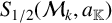
and, thus, we consider
$S_{1/2}(\mathcal {M}_k,a_{\mathbb {K}})$
 for a fixed k first. Following the argument of [Reference Fonga17, Lemma 2],

where the multiplicative function
$a_{\mathbb {K}}^\prime (n)$
 is defined by

It is clear that
$a_{\mathbb {K}}^\prime (p) = (\phi (d)+1)/2 \ge \phi (d)/2$
 for all primes p.
Let
$\mathcal {F}_k {:=}q \mathcal {F}_k(\ell ,\ell ^\prime )$
 denote the inner sum in (A.2). Set
$q=n_1d_1$
denote the inner sum in (A.2). Set
$q=n_1d_1$
 and
$q^\prime =n_1^\prime d_1$
and
$q^\prime =n_1^\prime d_1$
 , respectively. Then, choosing
$n=(q,q^\prime )$
, respectively. Then, choosing
$n=(q,q^\prime )$
 in the identity
$n=\sum _{d_1 \mid n}\phi (d_1)$
in the identity
$n=\sum _{d_1 \mid n}\phi (d_1)$
 , it follows that

Since every term in
$\mathcal {F}_k$
 is positive, it suffices to consider the case
$(n_1,n_1^\prime )=1$
is positive, it suffices to consider the case
$(n_1,n_1^\prime )=1$
 , which yields that

where

Note that
$\sigma (a_{\mathbb {K}}, R, r)$
 increases as R increases. Since
$\phi (d_1)/d_1 \gg 1$
increases as R increases. Since
$\phi (d_1)/d_1 \gg 1$
 as
$d_1\mid W$
as
$d_1\mid W$
 ,
,

Set
$\ell =n_2d_2$
 and
$\ell ^\prime =n_2^\prime d_2$
and
$\ell ^\prime =n_2^\prime d_2$
 . Applying the same calculation to the outer sum in (A.2),

Next, we estimate the lower bound for the above. Set

where
$\nu $
 is a bounded parameter. Restrict the previous outer sum to pairs
$(d_1,d_2)$
is a bounded parameter. Restrict the previous outer sum to pairs
$(d_1,d_2)$
 such that
$\omega (d_1),\omega (d_2)\le W_k/2-u_k$
such that
$\omega (d_1),\omega (d_2)\le W_k/2-u_k$
 , and the inner sum to integers
$n_2,n_2^\prime $
, and the inner sum to integers
$n_2,n_2^\prime $
 such that
${\omega (n_2)=\omega (n_2^\prime )=u_k}$
such that
${\omega (n_2)=\omega (n_2^\prime )=u_k}$
 . Combining with the fact that

we have

Proceeding as in the calculations of [Reference de la Bretèche and Tenenbaum12, pp. 8–9],

where

In fact, the Siegel–Walfisz theorem implies

Furthermore, noting that
$\omega (n_1^\prime d_1)+\omega (n_2 d_2) \le W_k$
 ,
,

Thus, (A.4) and (A.5) yield that

Together with the fact that

and Stirling’s formula, we obtain (A.3). A similar calculation yields

therefore, we have the following lower bound:

By performing a similar calculation again and noting that
$a_{\mathbb {K}}^\prime (p) = (\phi (d)+1)/2 \ge \phi (d)/2$
 ,
,

Substituting now into (A.6) shows that

Using the same calculation as [Reference de la Bretèche and Tenenbaum12, (2.13)],

Thus, combining this with (A.7),

where
$h {:=}q e^2 \beta \phi (d)(\sqrt {\alpha }-1)/(\sqrt {\alpha }+1)$
 .
.
Using (A.1) and the definition of
$w_k$
 ,
,

where
$\rho {:=}q 2 \delta \nu \log (h/\nu ^2)$
 . Setting
$v = \sqrt {h}/e$
. Setting
$v = \sqrt {h}/e$
 gives
gives

By choosing
$\beta \delta \log \alpha \to 1$
 and
$\alpha \to 1$
and
$\alpha \to 1$
 , we finish the proof of Proposition 3.1.
Acknowledgments
The authors are grateful to the referee for their careful reading, and valuable comments and suggestions, which definitely improve the readability and quality of this article. The authors would like to thank Dr. Winston Heap for his corrections to the manuscript. We also thank Dr. Zikang Dong and Dr. Guang-Liang Zhou for their valuable comments on our manuscript. The second author acknowledges the support of the China Scholarship Council program (Project ID: 202506260143). The third author is supported by the Natural Science Foundation of Henan Province (Grant No. 252300421782).



