


Overview
Assume that there is a box at each integer
 $x\in \mathbb {Z}$
and that each box may contain a ball or be empty. Denote
$x\in \mathbb {Z}$
and that each box may contain a ball or be empty. Denote
 $\eta \in \{0,1\}^{\mathbb {Z}}$
a ball configuration, with the convention
$\eta \in \{0,1\}^{\mathbb {Z}}$
a ball configuration, with the convention
 $\eta (x):= 1$
if there is a ball at x, else
$\eta (x):= 1$
if there is a ball at x, else
 $\eta (x):= 0$
. Imagine a carrier that traverses
$\eta (x):= 0$
. Imagine a carrier that traverses
 $ \mathbb {Z} $
from left to right as follows. When visiting box x, the carrier picks a ball if there is one and deposits a ball if the box
$ \mathbb {Z} $
from left to right as follows. When visiting box x, the carrier picks a ball if there is one and deposits a ball if the box
 $ x $
is empty and the carrier has at least one ball. Let
$ x $
is empty and the carrier has at least one ball. Let
 $T\eta $
be the configuration obtained after the carrier visited all boxes. An example of
$T\eta $
be the configuration obtained after the carrier visited all boxes. An example of
 $\eta $
, carrier load, and
$\eta $
, carrier load, and
 $T\eta $
is as follows:
$T\eta $
is as follows:
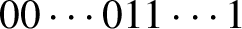
 $$ \begin{align*} \begin{array}{ll} \texttt{...0 0 0 1 0 1 1 0 0 0 0 1 1 0 1 0 0 0 0 0} &\eta\\ \ \texttt{...0 0 0 1 0 1 2 1 0 0 0 1 2 1 2 1 0 0 0} &\text{carrier load} \\ \texttt{...0 0 0 0 1 0 0 1 1 0 0 0 0 1 0 1 1 0 0 0 } &T\eta \end{array} \end{align*} $$
The map T for a general
 $ \eta \in \{0,1\}^{\mathbb {Z}} $
is defined in (1.2). This dynamics is called the box-ball system (BBS) and was introduced by Takahashi and Satsuma [Reference Takahashi and SatsumaTS90], who proposed an algorithm to identify solitons in configurations with a finite number of balls and argued that each soliton identified at time 0 can be tracked at successive iterations of T. For example, in the configuration having exactly three balls at boxes 1, 2, 3 the
$ \eta \in \{0,1\}^{\mathbb {Z}} $
is defined in (1.2). This dynamics is called the box-ball system (BBS) and was introduced by Takahashi and Satsuma [Reference Takahashi and SatsumaTS90], who proposed an algorithm to identify solitons in configurations with a finite number of balls and argued that each soliton identified at time 0 can be tracked at successive iterations of T. For example, in the configuration having exactly three balls at boxes 1, 2, 3 the
 $3$
-soliton
$3$
-soliton
 $\gamma $
consists of these three occupied boxes and the empty boxes 4, 5, 6. Evolving this configuration by t iterations of T, the new configuration will have a
$\gamma $
consists of these three occupied boxes and the empty boxes 4, 5, 6. Evolving this configuration by t iterations of T, the new configuration will have a
 $3$
-soliton
$3$
-soliton
 $\gamma ^t$
that is a translation of
$\gamma ^t$
that is a translation of
 $\gamma $
by
$\gamma $
by
 $3t$
. In general, [Reference Takahashi and SatsumaTS90] observed that a k-soliton always consists of k occupied boxes and k empty boxes. The relative positions can change and be more scattered during collisions with other solitons, but the striking property of the BBS is that such collisions neither create nor destroy solitons. The distance between solitons of the same size is also conserved after collisions.
$3t$
. In general, [Reference Takahashi and SatsumaTS90] observed that a k-soliton always consists of k occupied boxes and k empty boxes. The relative positions can change and be more scattered during collisions with other solitons, but the striking property of the BBS is that such collisions neither create nor destroy solitons. The distance between solitons of the same size is also conserved after collisions.
The main goal of [Reference Takahashi and SatsumaTS90] was to propose an integrable system with the same behavior as the Korteweg-de Vries equation, KdV, whose solutions include solitons of different sizes that keep shape after collision with other solitons. Then [Reference Tokihiro, Takahashi, Matsukidaira and SatsumaTTMS96, Reference Takahashi and MatsukidairaTM97] argued a way to go from KdV to BBS via ultradiscretisation and tropical geometry; see also [Reference Kato, Tsujimoto and ZukKTZ17, Reference ZukZuk20]. Further use of Bethe ansatz to study asymptotic behavior of BBS can be found in [Reference Inoue, Kuniba and OkadoIKO04, Reference Mada, Idzumi and TokihiroMIT06, Reference Inoue, Kuniba and TakagiIKT12, Reference Kuniba, Lyu and OkadoKLO18]. The model has also attracted attention in the combinatorics and probability communities. Using a map between solitons and Dick paths in [Reference Torii, Takahashi and SatsumaTTS96], the paper [Reference Levine, Lyu and PikeLLP17] relates soliton sizes to longest decreasing subsequence of restricted permutations. [Reference Ferrari and GabrielliFG20b] found a new soliton identification that maps to a branch decomposition of the Neveu-Aldous trees of random walks. See [Reference Lam, Pylyavsky and SakamotoLPS21, Reference SakamotoSak14a, Reference SakamotoSak14b] for some other combinatorial developments. The paper [Reference Hambly, Martin and O’ConnellHMO01] shows that stationary Markov chains are invariant measures for the Pitman transformation [Reference PitmanPit75], a dynamics equivalent to BBS; see [Reference Croydon, Kato, Sasada and TsujimotoCKST18, Reference Croydon and SasadaCS19, Reference Croydon and SasadaCS20] for extensions.
This article has three main contributions. Firstly, we discover the following fact: any ball configuration
 $\eta $
with ball density less than
$\eta $
with ball density less than
 $\frac 12$
can be mapped to a family of soliton components,
$\frac 12$
can be mapped to a family of soliton components,
 $(\zeta _k)_{k\geqslant 1}$
, called the slot decomposition of
$(\zeta _k)_{k\geqslant 1}$
, called the slot decomposition of
 $\eta $
; here
$\eta $
; here
 $\zeta _k(i)$
represents the number of k-solitons at coordinate
$\zeta _k(i)$
represents the number of k-solitons at coordinate
 $i\in \mathbb {Z}$
of the kth component. The components of a ball configuration evolve linearly under
$i\in \mathbb {Z}$
of the kth component. The components of a ball configuration evolve linearly under
 $ T $
: component k moves rigidly at speed k. The interaction among components reappears when the ball configuration is reconstructed from the components. This is a delicate hierarchical arrangement where the kth component is appended to a certain subset of
$ T $
: component k moves rigidly at speed k. The interaction among components reappears when the ball configuration is reconstructed from the components. This is a delicate hierarchical arrangement where the kth component is appended to a certain subset of
 $\mathbb {Z}$
called k-slots, determined by the m-components for
$\mathbb {Z}$
called k-slots, determined by the m-components for
 $m>k$
. The above facts are purely deterministic. It would be interesting to understand the relationship between the rigged configurations in [Reference Inoue, Kuniba and OkadoIKO04] with the slot decomposition.
$m>k$
. The above facts are purely deterministic. It would be interesting to understand the relationship between the rigged configurations in [Reference Inoue, Kuniba and OkadoIKO04] with the slot decomposition.
The BBS can be seen as a dynamical system acting on the set of configurations with density less than
 $ \frac {1}{2} $
, and a natural question is about the invariant measures
$ \frac {1}{2} $
, and a natural question is about the invariant measures
 $\mu $
defined by
$\mu $
defined by
 $\mu T^{-1} =\mu $
. Our second main result states that given a translation-invariant random family
$\mu T^{-1} =\mu $
. Our second main result states that given a translation-invariant random family
 $\zeta $
of independent vectors satisfying a summability condition, the law of the random ball configuration whose slot decomposition is
$\zeta $
of independent vectors satisfying a summability condition, the law of the random ball configuration whose slot decomposition is
 $\zeta $
is translation invariant and invariant for the BBS. Product measures and stationary Markov chains with density less than
$\zeta $
is translation invariant and invariant for the BBS. Product measures and stationary Markov chains with density less than
 $\frac 12$
satisfy those properties, as well as a large family of measures based on soliton weights [Reference Ferrari and GabrielliFG20a]. We conjecture that the slot decomposition characterises T-invariant probability measures in the sense that if
$\frac 12$
satisfy those properties, as well as a large family of measures based on soliton weights [Reference Ferrari and GabrielliFG20a]. We conjecture that the slot decomposition characterises T-invariant probability measures in the sense that if
 $\mu $
is shift-mixing and T-invariant, then its components should be independent and shift-mixing; see Remark 4.8.
$\mu $
is shift-mixing and T-invariant, then its components should be independent and shift-mixing; see Remark 4.8.
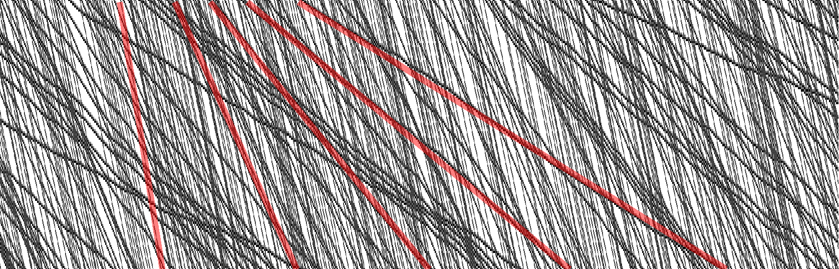
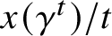
Our third main contribution is the characterisation of the effective soliton speeds for shift-ergodic initial states, illustrated by the red lines in the figure in the abstract. The result is based on the following rough description of the soliton dynamics. A size k soliton travels at speed k in absence of other solitons and when two solitons collide, the smaller soliton gets delayed and the bigger soliton ‘jumps’ over the slower one. Our proof is based on shift-ergodicity and Palm theory and does not use the slot decomposition. For a nonhomogeneous initial condition, the effective speed equations have been derived by [Reference Croydon and SasadaCS21], who also performed a hydrodynamic limit, using our slot decomposition. The results are analogous to those for the hard rod system [Reference Boldrighini, Dobrushin and SukhovBDS83], where disjoint segments of fixed size of the real line called rods travel ballistically at assigned speeds until collision, when the speeds are interchanged. A pulse follows the rod that is travelling at one of the given speeds. Hard rod pulses and BBS solitons have a similar dynamics and, consequently, similar hydrodynamic and effective speed equations. These results belong to the very active area of generalised hydrodynamics of the generalised Gibbs ensemble; see [Reference SpohnSpo12, Reference Doyon and SpohnDS17, Reference Doyon, Yoshimura and CauxDYC18, Reference Cao, Bulchandani and SpohnCBS19, Reference Kuniba, Misguich and PasquierKMP20] and references therein.
This article is organised as follows. In Section 1 we state the main results of this article, after giving the definitions needed for the statements. In Section 2 we introduce the slot decomposition of ball configurations, show that the slot decomposition is an injective map (Theorem 1.3) and describe how a configuration can be reconstructed from the components. In Section 3 we show that under the BBS dynamics each component shifts rigidly (Theorems 1.4 and 3.1). In Section 4 we give an explicit construction of T-invariant measures that are shift-invariant (Theorem 1.5). In Section 5 we compile fragments of Palm theory from the literature that play an important role in many of our arguments. In Section 6 we study the asymptotic speed of tagged solitons (Theorems 1.1 and 1.2). We also study the soliton speeds in terms of tagged records (Theorem 6.1). In Section 7 we complete some proofs postponed in previous sections.
1 Preliminaries and results
In this section we describe our main results. We will work mostly with configurations with ball density less than
 $\frac 12$
. More precisely, let
$\frac 12$
. More precisely, let

In the sequel, a site
 $x\in \mathbb {Z}$
is often referred to as a box. For
$x\in \mathbb {Z}$
is often referred to as a box. For
 $\eta \in \mathcal {X}$
we define the set of records by
$\eta \in \mathcal {X}$
we define the set of records by
 $$ \begin{align} R\eta := \Big\{ x\in \mathbb{Z} : \sum_{y=z}^x \eta(y) < \sum_{y=z}^x [1-\eta(y)] \text{ for all } z\leqslant x \Big\}. \end{align} $$
Note that
 $ \eta (x)=0 $
for all
$ \eta (x)=0 $
for all
 $ x \in R\eta $
. The piece of configuration between two consecutive records forms a finite excursion. The operator T is defined by
$ x \in R\eta $
. The piece of configuration between two consecutive records forms a finite excursion. The operator T is defined by
 $$ \begin{align} T\eta(x) := \begin{cases} 0,& x \in R\eta, \\ 1-\eta(x),& \text{otherwise}. \end{cases} \end{align} $$
In other words, the value at records remains 0 and the excursions are flipped. When applied to finite ball configurations, this operator coincides with the operator described in the previous section. We show in Section 2 that if
 $\lambda <\frac 12$
then
$\lambda <\frac 12$
then
 $\mathcal {X}_\lambda $
is invariant under T.
$\mathcal {X}_\lambda $
is invariant under T.
1.1 Identifying and tracking solitons
Define the runs of
 $\eta $
as maximal blocks of successive sites where
$\eta $
as maximal blocks of successive sites where
 $\eta $
has a constant value, so that they form a partition of
$\eta $
has a constant value, so that they form a partition of
 $\mathbb {Z}$
. Assume first that
$\mathbb {Z}$
. Assume first that
 $\eta $
has a finite number of balls, so it has a finite number of finite runs and two semi-infinite runs of zeros, one to the left and one to the right.
$\eta $
has a finite number of balls, so it has a finite number of finite runs and two semi-infinite runs of zeros, one to the left and one to the right.
A k-soliton is a collection of
 $2k$
boxes identified by the Takahashi–Satsuma algorithm [Reference Takahashi and SatsumaTS90] running as follows.
$2k$
boxes identified by the Takahashi–Satsuma algorithm [Reference Takahashi and SatsumaTS90] running as follows.

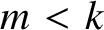
Notice that a k-soliton consists of k zeros (possibly nonconsecutive) followed by k ones or vice versa, and letters that do not belong to any soliton are all zero and correspond to the records of
 $\eta $
; see Figure 1.1. For a general
$\eta $
; see Figure 1.1. For a general
 $\eta \in \mathcal {X}$
, all excursions have a finite number of boxes. To identify the solitons in
$\eta \in \mathcal {X}$
, all excursions have a finite number of boxes. To identify the solitons in
 $\eta $
, we take each excursion of
$\eta $
, we take each excursion of
 $\eta $
, append infinitely many zeros to the left and right of the excursion and then apply the above algorithm to it.
$\eta $
, append infinitely many zeros to the left and right of the excursion and then apply the above algorithm to it.
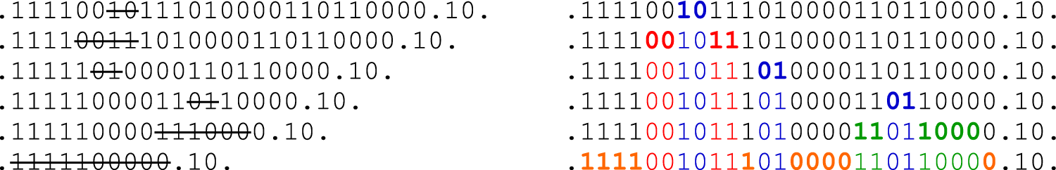
Applying the Takahashi–Satsuma algorithm to a sample configuration. Dots represent records. On the left we have the resulting word after successive iterations. Identified solitons are shown in bold once and then with a color corresponding to their size. The algorithm is applied to each excursion separately, so the rightmost
 $1$
-soliton in the picture is ignored by this instance of the procedure. (color online)
$1$
-soliton in the picture is ignored by this instance of the procedure. (color online)
We define the head and tail of a k-soliton
 $\gamma $
as follows: the head
$\gamma $
as follows: the head
 $\mathcal {H}(\gamma )=\{\mathcal {H}_{1}, \mathcal {H}_{2}, \dots, \mathcal {H}_{k}\}\subseteq \mathbb {Z}$
is the set of k boxes with ones in
$\mathcal {H}(\gamma )=\{\mathcal {H}_{1}, \mathcal {H}_{2}, \dots, \mathcal {H}_{k}\}\subseteq \mathbb {Z}$
is the set of k boxes with ones in
 $\gamma $
and the tail
$\gamma $
and the tail
 $\mathcal {T}(\gamma )=\{\mathcal {T}_{1}, \mathcal {T}_{2}, \dots, \mathcal {T}_{k}\}\subseteq \mathbb {Z}$
is the set of k boxes with zeroes in
$\mathcal {T}(\gamma )=\{\mathcal {T}_{1}, \mathcal {T}_{2}, \dots, \mathcal {T}_{k}\}\subseteq \mathbb {Z}$
is the set of k boxes with zeroes in
 $\gamma $
. Namely,
$\gamma $
. Namely,
 $\mathcal {H}(\gamma )\cup \mathcal {T}(\gamma )$
is the set of boxes that are removed when executing the previous algorithm on
$\mathcal {H}(\gamma )\cup \mathcal {T}(\gamma )$
is the set of boxes that are removed when executing the previous algorithm on
 $\eta $
. Let
$\eta $
. Let
 $\Gamma _k\eta $
be the set of k-solitons of a ball configuration
$\Gamma _k\eta $
be the set of k-solitons of a ball configuration
 $\eta \in \mathcal {X}$
. The following is proved in Section 7.
$\eta \in \mathcal {X}$
. The following is proved in Section 7.
Proposition 1.3. For any
 $\eta \in \mathcal {X}$
and
$\eta \in \mathcal {X}$
and
 $A \subseteq \mathbb {Z}$
, there is a k-soliton
$A \subseteq \mathbb {Z}$
, there is a k-soliton
 $\gamma \in \Gamma _k\eta $
with tail
$\gamma \in \Gamma _k\eta $
with tail
 $\mathcal {T}(\gamma )=A$
if and only if there is a k-soliton
$\mathcal {T}(\gamma )=A$
if and only if there is a k-soliton
 $\gamma ^1 \in \Gamma _k(T\eta )$
with head
$\gamma ^1 \in \Gamma _k(T\eta )$
with head
 $\mathcal {H}(\gamma ^1) = A$
.
$\mathcal {H}(\gamma ^1) = A$
.
By the above proposition, we can track each k-soliton
 $\gamma $
in the evolution of
$\gamma $
in the evolution of
 $\eta $
. For each k-soliton
$\eta $
. For each k-soliton
 $\gamma \in \Gamma _k \eta $
, call
$\gamma \in \Gamma _k \eta $
, call
 $(\gamma ^t)_{t\geqslant 0}$
the trajectory satisfying
$(\gamma ^t)_{t\geqslant 0}$
the trajectory satisfying
 $\gamma ^0 =\gamma $
,
$\gamma ^0 =\gamma $
,
 $\gamma ^t\in \Gamma _kT^t\eta $
and
$\gamma ^t\in \Gamma _kT^t\eta $
and
 $$ \begin{align} \mathcal{H}(\gamma^{t+1}) = \mathcal{T}(\gamma^t). \end{align} $$
1.2 Soliton nesting and motion
As shown in Figure 1.1, solitons can be nested inside larger solitons. As it turns out, they are nested in a hierarchical way. Moreover, solitons only move to the right, and they are only free to move when they are not nested inside larger solitons. In particular, solitons can only overtake smaller solitons. We now make these statements precise.
Let
 $ \gamma \in \Gamma _k \eta $
for some
$ \gamma \in \Gamma _k \eta $
for some
 $ k\in \mathbb {N} $
. Let us denote by
$ k\in \mathbb {N} $
. Let us denote by
 $x(\gamma )$
its leftmost site. Take
$x(\gamma )$
its leftmost site. Take
 $ z $
as the first site to the right of
$ z $
as the first site to the right of
 $ \gamma $
such that
$ \gamma $
such that
 $ z $
is either a record or belongs to another
$ z $
is either a record or belongs to another
 $ m $
-soliton for some
$ m $
-soliton for some
 $ m \geqslant k $
. The interval spanned by
$ m \geqslant k $
. The interval spanned by
 $ \gamma $
is defined as
$ \gamma $
is defined as
 $ I(\gamma ) := [x(\gamma ),z-1] \cap \mathbb {Z} $
.
$ I(\gamma ) := [x(\gamma ),z-1] \cap \mathbb {Z} $
.
Lemma 1.5. Let
 $ \gamma \in \Gamma _k \eta $
. Then both the head and tail of
$ \gamma \in \Gamma _k \eta $
. Then both the head and tail of
 $ \gamma $
are contained in
$ \gamma $
are contained in
 $ I(\gamma ) $
. Also,
$ I(\gamma ) $
. Also,
 $I(\gamma )$
does not contain any record, nor any site that belongs to the head or tail of another
$I(\gamma )$
does not contain any record, nor any site that belongs to the head or tail of another
 $ m $
-soliton with
$ m $
-soliton with
 $ m \geqslant k $
. Moreover, if
$ m \geqslant k $
. Moreover, if
 $\gamma ' \in \Gamma _m \eta $
with
$\gamma ' \in \Gamma _m \eta $
with
 $m> k$
is such that
$m> k$
is such that
 $I(\gamma )\cap I(\gamma ')\ne \varnothing $
, then
$I(\gamma )\cap I(\gamma ')\ne \varnothing $
, then
 $I(\gamma )\subseteq I(\gamma ')$
. If
$I(\gamma )\subseteq I(\gamma ')$
. If
 $\gamma $
and
$\gamma $
and
 $\gamma '$
are two different k solitons, then
$\gamma '$
are two different k solitons, then
 $I(\gamma )\cap I(\gamma ')=\varnothing $
.
$I(\gamma )\cap I(\gamma ')=\varnothing $
.
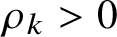
The interval
 $ I(\gamma ) $
and the above properties are illustrated in Figure 1.2.
$ I(\gamma ) $
and the above properties are illustrated in Figure 1.2.
Here we show
 $ I(\gamma ) $
in an example with nine records, a 5-soliton, a 4-soliton, two 3-solitons, two 2-solitons and two 1-solitons, with one color for each size. In this example, a 1-soliton is contained in a 2-soliton, both 2-solitons are contained in the 5-soliton and both 3-solitons are contained in the 4-soliton.
$ I(\gamma ) $
in an example with nine records, a 5-soliton, a 4-soliton, two 3-solitons, two 2-solitons and two 1-solitons, with one color for each size. In this example, a 1-soliton is contained in a 2-soliton, both 2-solitons are contained in the 5-soliton and both 3-solitons are contained in the 4-soliton.
 $ I(\gamma ) $
is underlined with the same color as
$ I(\gamma ) $
is underlined with the same color as
 $ \gamma $
, and black zeros are records. (color online)
$ \gamma $
, and black zeros are records. (color online)

Recall the notation
 $\gamma ^{1}$
from Proposition 1.3. The following lemma says that a soliton can move forward only if it is not already nested inside a larger one.
$\gamma ^{1}$
from Proposition 1.3. The following lemma says that a soliton can move forward only if it is not already nested inside a larger one.
Lemma 1.6. Let
 $ \gamma \in \Gamma _k \eta $
. If
$ \gamma \in \Gamma _k \eta $
. If
 $ I(\gamma ) \subseteq I(\gamma ') $
for some
$ I(\gamma ) \subseteq I(\gamma ') $
for some
 $ \gamma ' \in \Gamma _m\eta $
with
$ \gamma ' \in \Gamma _m\eta $
with
 $ m> k $
, then
$ m> k $
, then
 $\mathcal {T}(\gamma ^{1})=\mathcal {H}(\gamma )$
and
$\mathcal {T}(\gamma ^{1})=\mathcal {H}(\gamma )$
and
 $\mathcal {H}(\gamma ^{1})=\mathcal {T}(\gamma )$
; hence
$\mathcal {H}(\gamma ^{1})=\mathcal {T}(\gamma )$
; hence
 $ x(\gamma ^1) = x(\gamma ) $
. Otherwise,
$ x(\gamma ^1) = x(\gamma ) $
. Otherwise,
 $\mathcal {T}(\gamma ^{1}) \ne \mathcal {H}(\gamma )$
and
$\mathcal {T}(\gamma ^{1}) \ne \mathcal {H}(\gamma )$
and
 $ x(\gamma ^1)> x(\gamma ) $
.
$ x(\gamma ^1)> x(\gamma ) $
.
Our last observation is that smaller solitons never overtake larger ones.
Lemma 1.7. Let
 $ \eta \in \mathcal {X} $
and suppose that
$ \eta \in \mathcal {X} $
and suppose that
 $\gamma \in \Gamma _{k} \eta $
and
$\gamma \in \Gamma _{k} \eta $
and
 $\tilde \gamma \in \Gamma _{m} \eta $
for some
$\tilde \gamma \in \Gamma _{m} \eta $
for some
 $ m \geqslant k \geqslant 1 $
. If
$ m \geqslant k \geqslant 1 $
. If
 $x(\gamma )<x(\tilde \gamma )$
, then
$x(\gamma )<x(\tilde \gamma )$
, then
 $ x(\gamma ^{t}) < x(\tilde \gamma ^{t}) $
for all
$ x(\gamma ^{t}) < x(\tilde \gamma ^{t}) $
for all
 $ t\in \mathbb {N} $
.
$ t\in \mathbb {N} $
.
These three lemmas are also proved in Section 7.
1.3 Asymptotic speeds
We use
 $\theta $
to denote shift operators on
$\theta $
to denote shift operators on
 $ \mathbb {Z} $
, its power set
$ \mathbb {Z} $
, its power set
 $ \mathcal {P}(\mathbb {Z}) $
and
$ \mathcal {P}(\mathbb {Z}) $
and
 $ \{0,1\}^{\mathbb {Z}} $
. Namely,
$ \{0,1\}^{\mathbb {Z}} $
. Namely,
 $$ \begin{align} \theta x = x-1, \quad \theta A = \{\theta x : x\in A\}, \quad \theta\eta(y):= \eta(\theta^{-1} y) \text{ for } \eta\in \{0,1\}^{\mathbb{Z}}. \end{align} $$
Let
 $ \mathcal {B} $
denote the Borel
$ \mathcal {B} $
denote the Borel
 $ \sigma $
-field of
$ \sigma $
-field of
 $ \{0,1\}^{\mathbb {Z}} $
. We say that a probability measure
$ \{0,1\}^{\mathbb {Z}} $
. We say that a probability measure
 $\mu $
on
$\mu $
on
 $\{0,1\}^{\mathbb {Z}}$
is shift-ergodic if
$\{0,1\}^{\mathbb {Z}}$
is shift-ergodic if
 $\mu $
is
$\mu $
is
 $\theta $
-invariant and for every event
$\theta $
-invariant and for every event
 $A \in \mathcal {B}$
satisfying
$A \in \mathcal {B}$
satisfying
 $\theta ^{-1}(A)=A$
we have
$\theta ^{-1}(A)=A$
we have
 $\mu (A)=0$
or
$\mu (A)=0$
or
 $1$
. Let
$1$
. Let
 $\mu $
be a shift-ergodic measure on
$\mu $
be a shift-ergodic measure on
 $\mathcal {X}$
and denote by
$\mathcal {X}$
and denote by
 $\rho _k$
the mean number of k-solitons per excursion, by
$\rho _k$
the mean number of k-solitons per excursion, by
 $w_0=1+\sum _k 2k\rho _k$
the mean distance between records and by
$w_0=1+\sum _k 2k\rho _k$
the mean distance between records and by
 $\bar {\rho }_k = \frac {\rho _k}{w_0}$
the mean number of k-solitons per unit space (precise definitions in Subsection 4.3). Recall that
$\bar {\rho }_k = \frac {\rho _k}{w_0}$
the mean number of k-solitons per unit space (precise definitions in Subsection 4.3). Recall that
 $x(\gamma )$
is the leftmost site of a soliton
$x(\gamma )$
is the leftmost site of a soliton
 $\gamma $
and that
$\gamma $
and that
 $\gamma ^t$
is the soliton
$\gamma ^t$
is the soliton
 $\gamma $
at time t. We now state the main result concerning soliton speeds.
$\gamma $
at time t. We now state the main result concerning soliton speeds.
Theorem 1.1. Let
 $\mu $
be a T-invariant and shift-ergodic measure on
$\mu $
be a T-invariant and shift-ergodic measure on
 $\mathcal {X}$
. Then there exist deterministic speeds
$\mathcal {X}$
. Then there exist deterministic speeds
 $(v_k)_k$
such that
$(v_k)_k$
such that
 $\mu $
-almost surely (a.s.) for all
$\mu $
-almost surely (a.s.) for all
 $k\geqslant 1$
and
$k\geqslant 1$
and
 $\gamma \in \Gamma _k\eta $
,
$\gamma \in \Gamma _k\eta $
,
 $$ \begin{align} \lim_{t\to\infty} \frac{x(\gamma^t)}{t} &= v_k. \end{align} $$
The soliton speeds
 $ v_k $
are finite, positive, increasing in
$ v_k $
are finite, positive, increasing in
 $ k $
and satisfy the system
$ k $
and satisfy the system
 $$ \begin{align} v_k = k + \sum_{m<k} 2m \bar{\rho}_m (v_k-v_m) - \sum_{m>k} 2k \bar{\rho}_m (v_m-v_k). \end{align} $$
System (1.10) comes from the following. When a k-soliton is isolated, it advances by k units, and when it encounters an m soliton, the encounter causes it to advance
 $2m$
extra units if
$2m$
extra units if
 $m<k$
or stay put for two units of time if
$m<k$
or stay put for two units of time if
 $m>k$
. The term
$m>k$
. The term
 $\bar {\rho }_m |v_k-v_m|$
gives the frequency of such encounters as seen from a k-soliton.
$\bar {\rho }_m |v_k-v_m|$
gives the frequency of such encounters as seen from a k-soliton.
When
 $ \rho _k=0 $
, the soliton speed
$ \rho _k=0 $
, the soliton speed
 $ v_k $
does not come from (1.9) but in principle formally from (1.10). There is still an interpretation for
$ v_k $
does not come from (1.9) but in principle formally from (1.10). There is still an interpretation for
 $ v_k $
in terms of the dynamics, as discussed in Subsection 6.5.
$ v_k $
in terms of the dynamics, as discussed in Subsection 6.5.
When
 $\rho _k>0$
for finitely many
$\rho _k>0$
for finitely many
 $ k $
, the system has a unique solution [Reference Croydon and SasadaCS21, Lemma 5.1]. We believe it is unique in general, but we have been unable to prove it. The following partial result is proved in Section 7.
$ k $
, the system has a unique solution [Reference Croydon and SasadaCS21, Lemma 5.1]. We believe it is unique in general, but we have been unable to prove it. The following partial result is proved in Section 7.
Proposition 1.11. If
 $\sum _m m \bar {\rho }_m < \frac {1}{4}$
, then the nonnegative solution to (1.10) is unique.
$\sum _m m \bar {\rho }_m < \frac {1}{4}$
, then the nonnegative solution to (1.10) is unique.
As a side remark,
 $ \sum _m m \bar {\rho }_m = \lambda $
; that is, the mean number of occupied boxes per unit space. Uniqueness has not been proved to hold in general, and we show that
$ \sum _m m \bar {\rho }_m = \lambda $
; that is, the mean number of occupied boxes per unit space. Uniqueness has not been proved to hold in general, and we show that
 $(v_k)_k$
is determined by the vector
$(v_k)_k$
is determined by the vector
 $ (\bar {\rho }_k)_k $
under a stronger assumption in terms of soliton components (described in Subsection 1.5).
$ (\bar {\rho }_k)_k $
under a stronger assumption in terms of soliton components (described in Subsection 1.5).
Theorem 1.2. If, when conditioned on having a record at
 $ x=0 $
,
$ x=0 $
,
 $\mu $
has independent soliton components and each component is independent and identically distributed (i.i.d.), then the soliton speeds
$\mu $
has independent soliton components and each component is independent and identically distributed (i.i.d.), then the soliton speeds
 $(v_k)_k$
in (1.9) are also given by the unique solution to
$(v_k)_k$
in (1.9) are also given by the unique solution to
 $$ \begin{align} \begin{aligned} w_k&=1+\sum_{m>k} 2(m-k) \rho_m, & \rho_k &= \alpha_k w_k,\\ s_k &= k+\sum_{m<k}2(k-m) s_m \alpha_m, & v_k &= \frac {s_k}{w_k}, \end{aligned} \end{align} $$
and, in particular, they are determined by
 $(\rho _k)_k$
.
$(\rho _k)_k$
.
In system (1.12),
 $w_k$
is the density of k-slots per excursion (see Subsection 1.4 for the definition of k-slot),
$w_k$
is the density of k-slots per excursion (see Subsection 1.4 for the definition of k-slot),
 $\alpha _k$
is the density of k-solitons per k-slot,
$\alpha _k$
is the density of k-solitons per k-slot,
 $s_k$
is the average size of the head of a k-soliton,
$s_k$
is the average size of the head of a k-soliton,
 $k-m$
is the number of m-slots in the head of a k-soliton and the factor
$k-m$
is the number of m-slots in the head of a k-soliton and the factor
 $\frac {1}{w_k}$
is the probability that a typical k-soliton is free to move (see Section 6 for details).
$\frac {1}{w_k}$
is the probability that a typical k-soliton is free to move (see Section 6 for details).
The proof of (1.12) uses independence properties of the components for an explicit computation of the mean jump size of a typical k-soliton
 $\gamma $
in one iteration. By ergodicity, the mean jump size is
$\gamma $
in one iteration. By ergodicity, the mean jump size is
 $v_k$
, the limit of
$v_k$
, the limit of
 $x(\gamma ^t)/t$
, as shown in Subsection 6.1.
$x(\gamma ^t)/t$
, as shown in Subsection 6.1.
In the setup of Theorem 1.1, we cannot compute the mean jump size explicitly. However, if we assume that the solution to (1.10) is indeed unique, then by taking an initial measure with independent components and the same vector
 $ (\rho _k)_k $
, we see that the vector
$ (\rho _k)_k $
, we see that the vector
 $ (v_k)_k $
must be given by (1.12). So if the solution to (1.10) is indeed unique (as conjectured), the independence assumption in Theorem 1.2 can be waived.
$ (v_k)_k $
must be given by (1.12). So if the solution to (1.10) is indeed unique (as conjectured), the independence assumption in Theorem 1.2 can be waived.
In practice, the soliton speeds
 $(v_k)_{k}$
can be computed by truncating
$(v_k)_{k}$
can be computed by truncating
 $\rho $
(replace
$\rho $
(replace
 $\rho _k$
by
$\rho _k$
by
 $0$
for large k) and solving these finite recursions for w,
$0$
for large k) and solving these finite recursions for w,
 $\alpha $
, s and finally v. When the initial ball configuration consists of i.i.d. Bernoulli random variables, one can find
$\alpha $
, s and finally v. When the initial ball configuration consists of i.i.d. Bernoulli random variables, one can find
 $\alpha _k$
explicitly in terms of the density
$\alpha _k$
explicitly in terms of the density
 $\lambda $
by computing partition functions [Reference Ferrari and GabrielliFG20a], substitute the equation for
$\lambda $
by computing partition functions [Reference Ferrari and GabrielliFG20a], substitute the equation for
 $\rho $
into that for w and then compute s and v. Using this and the above theorem, we have found the asymptotic speeds of the solitons for the simulations shown in Figures 1.3 and 1.4 as well as that on the first page.
$\rho $
into that for w and then compute s and v. Using this and the above theorem, we have found the asymptotic speeds of the solitons for the simulations shown in Figures 1.3 and 1.4 as well as that on the first page.
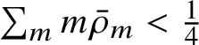
Simulation for an i.i.d. configuration with density
 $0.15$
. The transparent red lines have deterministic slopes computed by Theorem 1.2, which have been manually shifted so that they would overlay a soliton. This window covers 2000 sites and 140 time steps going downwards and has been stretched vertically by a factor of
$0.15$
. The transparent red lines have deterministic slopes computed by Theorem 1.2, which have been manually shifted so that they would overlay a soliton. This window covers 2000 sites and 140 time steps going downwards and has been stretched vertically by a factor of
 $5$
. The figure on the first page is the same except for the density. (high resolution, color online)
$5$
. The figure on the first page is the same except for the density. (high resolution, color online)

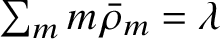
Simulation for
 $(\rho _k)_k=(.006,.005,.1,.003,0,0,0,\dots )$
. The initial configuration was obtained by first appending one k-soliton with probability
$(\rho _k)_k=(.006,.005,.1,.003,0,0,0,\dots )$
. The initial configuration was obtained by first appending one k-soliton with probability
 $\rho _k$
after each record and then applying T a number of times in order to mix. As in Figure 1.3, it is a 2000 x 140 window stretched by 5, and red lines are deterministic. (high resolution, color online)
$\rho _k$
after each record and then applying T a number of times in order to mix. As in Figure 1.3, it is a 2000 x 140 window stretched by 5, and red lines are deterministic. (high resolution, color online)
1.4 Slot decomposition
Recall that a k-soliton has a head and a tail, each one consisting of k (possibly nonconsecutive) sites. We say that the jth box of the head or tail of an m-soliton is a k-slot for all
 $k<j$
and that a record is a k-slot for every k. Roughly speaking, the k-slots are the places where k-solitons can be appended; see Subsection 2.1 for precise definitions and examples.
$k<j$
and that a record is a k-slot for every k. Roughly speaking, the k-slots are the places where k-solitons can be appended; see Subsection 2.1 for precise definitions and examples.
The set of configurations with a record at the origin is defined by
 $$ \begin{align*} \skew8\widehat{\mathcal{X}}:=\{\eta\in\mathcal{X}:0\in R\eta\}. \end{align*} $$
Assume that
 $\eta \in \skew8\widehat{\mathcal {X}}$
. Enumerate the k-slots from left to right such that the
$\eta \in \skew8\widehat{\mathcal {X}}$
. Enumerate the k-slots from left to right such that the
 $0$
th k-slot is at position
$0$
th k-slot is at position
 $s_k(\eta,0)=0$
, and let
$s_k(\eta,0)=0$
, and let
 $s_k(\eta,i)$
denote the position of the ith k-slot for
$s_k(\eta,i)$
denote the position of the ith k-slot for
 $i\in \mathbb {Z}$
. We say that a k-soliton
$i\in \mathbb {Z}$
. We say that a k-soliton
 $\gamma $
is appended to the ith k-slot if its head and tail are contained between
$\gamma $
is appended to the ith k-slot if its head and tail are contained between
 $s_k(\eta,i)$
and
$s_k(\eta,i)$
and
 $s_k(\eta,i+1)$
. Define the kth component of
$s_k(\eta,i+1)$
. Define the kth component of
 $\eta $
as the configuration
$\eta $
as the configuration
 $M_k\eta $
given by M
k
$M_k\eta $
given by M
k
 $\eta $
(i):= number of k-solitons appended to the ith k-slot. Define
$\eta $
(i):= number of k-solitons appended to the ith k-slot. Define
 $$ \begin{align*} \mathcal{M}:=\bigl\{\zeta= (\zeta_k)_{k\geqslant1}, \,\zeta_k \in (\mathbb{Z}_+)^{\mathbb{Z}}: \textstyle{\sum}_k \zeta_k(i)<\infty,\,\text{ for all }i\in\mathbb{Z}\bigr\}. \end{align*} $$
The next result, proved in Subsection 2.2, says that we can recover
 $\eta $
from its components
$\eta $
from its components
 $(M_{k}\eta )_{k}$
.
$(M_{k}\eta )_{k}$
.
Theorem 1.3. For
 $\eta \in \skew8\widehat{\mathcal {X}}$
, we have
$\eta \in \skew8\widehat{\mathcal {X}}$
, we have
 $(M_{k}\eta )_{k}\in \mathcal {M}$
. Moreover, the map
$(M_{k}\eta )_{k}\in \mathcal {M}$
. Moreover, the map
 $M:\eta \in \skew8\widehat{\mathcal {X}}\mapsto (M_k\eta )_k$
is invertible.
$M:\eta \in \skew8\widehat{\mathcal {X}}\mapsto (M_k\eta )_k$
is invertible.
The fundamental property of this decomposition is that it makes the BBS dynamics linear. We show a simple case, deferring the full statement until Theorem 3.1 in Section 3.
Theorem 1.4. Suppose
 $ \eta \equiv 0 $
on
$ \eta \equiv 0 $
on
 $ \mathbb {Z}_- $
and
$ \mathbb {Z}_- $
and
 $ \eta $
has infinitely many records on
$ \eta $
has infinitely many records on
 $ \mathbb {Z}_+ $
. Then for all
$ \mathbb {Z}_+ $
. Then for all
 $k\geqslant 1$
,
$k\geqslant 1$
,
 $$ \begin{align*} M_k T\eta =\theta^{-k} M_k\eta. \end{align*} $$
So, when we see a configuration
 $ \eta $
through its components, the kth component is displaced by k units, without interacting with the other components. In the general case, there will be larger solitons arriving from the left, which will disrupt the enumeration of k-slots, making the statement substantially more involved. See the details in Section 3.
$ \eta $
through its components, the kth component is displaced by k units, without interacting with the other components. In the general case, there will be larger solitons arriving from the left, which will disrupt the enumeration of k-slots, making the statement substantially more involved. See the details in Section 3.
1.5 Invariant measures
Using the slot decomposition and the reconstruction map
 $(M_{k}\eta )_{k}\mapsto \eta $
that will be described in detail in Subsection 2.2, we get the following.
$(M_{k}\eta )_{k}\mapsto \eta $
that will be described in detail in Subsection 2.2, we get the following.
Theorem 1.5. Let
 $\zeta =(\zeta _k)_{k\geqslant 1}$
be independent random elements of
$\zeta =(\zeta _k)_{k\geqslant 1}$
be independent random elements of
 $(\mathbb {Z}_{+})^{\mathbb {Z}}$
with shift-invariant distributions satisfying
$(\mathbb {Z}_{+})^{\mathbb {Z}}$
with shift-invariant distributions satisfying
 $\sum _k k E[\zeta _k(0)] <\infty $
and
$\sum _k k E[\zeta _k(0)] <\infty $
and
 $P(\sum _{k,i}\zeta _{k}(i)>0)=1$
. Then there exists a unique shift-invariant probability
$P(\sum _{k,i}\zeta _{k}(i)>0)=1$
. Then there exists a unique shift-invariant probability
 $\mu $
on
$\mu $
on
 $\mathcal {X}$
such that
$\mathcal {X}$
such that
 $M_k \eta \overset {d}{=}\zeta _k$
when
$M_k \eta \overset {d}{=}\zeta _k$
when
 $\eta $
is distributed with
$\eta $
is distributed with
 $\mu $
conditioned on
$\mu $
conditioned on
 $ \skew8\widehat{\mathcal {X}} $
. This measure
$ \skew8\widehat{\mathcal {X}} $
. This measure
 $\mu $
is T-invariant. If, moreover,
$\mu $
is T-invariant. If, moreover,
 $(\zeta _k(i))_{i\in \mathbb {Z}}$
is i.i.d. for each k, then
$(\zeta _k(i))_{i\in \mathbb {Z}}$
is i.i.d. for each k, then
 $\mu $
is also shift-ergodic.
$\mu $
is also shift-ergodic.
The above theorem says that the family of invariant measures for this dynamics is at least as large as the family of sequences of states of k-soliton configurations. In particular, given a sequence
 $(\alpha _k)_k$
specifying the density of k-solitons in the kth component, we can construct an infinite number of mutually singular shift-invariant and T-invariant laws
$(\alpha _k)_k$
specifying the density of k-solitons in the kth component, we can construct an infinite number of mutually singular shift-invariant and T-invariant laws
 $\mu $
on
$\mu $
on
 $\mathcal {X}$
, all having the same specified component densities.
$\mathcal {X}$
, all having the same specified component densities.
The extra assumption needed in Theorem 1.2 is that
 $\mu $
be of the above form; that is, conditioning on
$\mu $
be of the above form; that is, conditioning on
 $ \skew8\widehat{\mathcal {X}} $
, each kth component is i.i.d. and they are independent over k. In this case, we can also study the speed of tagged records and the speed of solitons measured in terms of tagged records; see Subsection 6.5. As pointed out above, this condition should not be necessary for Theorem 1.2 to hold.
$ \skew8\widehat{\mathcal {X}} $
, each kth component is i.i.d. and they are independent over k. In this case, we can also study the speed of tagged records and the speed of solitons measured in terms of tagged records; see Subsection 6.5. As pointed out above, this condition should not be necessary for Theorem 1.2 to hold.
We should also note that the converse of Theorem 1.5 is false. In particular, there exist invariant measures that are not constructed from independent components; see Examples 4.6 and 4.7 as well as Remark 4.8 in Subsection 4.1.
2 Slot decomposition
Let
 $\xi =\xi [\eta ]$
be a walk on
$\xi =\xi [\eta ]$
be a walk on
 $\mathbb {Z}$
that jumps one unit up at x when there is a ball at x and jumps one unit down when box x is empty. That is,
$\mathbb {Z}$
that jumps one unit up at x when there is a ball at x and jumps one unit down when box x is empty. That is,
 $$ \begin{align*} \xi(x)-\xi(x-1) = 2\eta(x)-1. \end{align*} $$
Note that for each
 $\eta $
, such a walk
$\eta $
, such a walk
 $\xi [\eta ]$
is not unique and only defined up to a vertical shift. We define records for a walk
$\xi [\eta ]$
is not unique and only defined up to a vertical shift. We define records for a walk
 $\xi $
in the usual sense; that is, we say that x is a record for
$\xi $
in the usual sense; that is, we say that x is a record for
 $\xi $
if
$\xi $
if
 $\xi (z)> \xi (x)$
for all
$\xi (z)> \xi (x)$
for all
 $z<x$
. Let
$z<x$
. Let
 $ \mathcal {W}_\lambda $
be the set of all simple walks
$ \mathcal {W}_\lambda $
be the set of all simple walks
 $ \xi $
such that
$ \xi $
such that
 $ \eta [\xi ] \in \mathcal {X}_\lambda $
, which is the set of walks
$ \eta [\xi ] \in \mathcal {X}_\lambda $
, which is the set of walks
 $ \xi $
such that
$ \xi $
such that
 $$ \begin{align} \lim_{x\to\pm\infty} \frac{\xi(x)}{x} = 2 \lambda - 1, \end{align} $$
and
 $\mathcal {W} = \cup _{0< \lambda <1/2 }\mathcal {W}_{\lambda }$
. Then every
$\mathcal {W} = \cup _{0< \lambda <1/2 }\mathcal {W}_{\lambda }$
. Then every
 $\xi \in \mathcal {W}$
satisfies
$\xi \in \mathcal {W}$
satisfies
 $\min \limits _{y\leqslant x}\xi (y) \in \mathbb {Z}$
for all
$\min \limits _{y\leqslant x}\xi (y) \in \mathbb {Z}$
for all
 $x \in \mathbb {Z}$
, and we define
$x \in \mathbb {Z}$
, and we define
 $$ \begin{align} T\xi(x) := 2 \min_{y\leqslant x} \xi(y) - \xi(x) = \big[\min_{y\leqslant x}\xi(y)\big]-\Big[\xi(x)-\min_{y\leqslant x}\xi(y)\Big]. \end{align} $$
This amounts to reflecting the walk
 $\xi $
with respect to its running minimum. It is worth mentioning that the above transformation for Brownian motion was studied by Pitman [Reference PitmanPit75]. The way that T acts on
$\xi $
with respect to its running minimum. It is worth mentioning that the above transformation for Brownian motion was studied by Pitman [Reference PitmanPit75]. The way that T acts on
 $\mathcal {W}$
is illustrated with an example in Figure 2.1.
$\mathcal {W}$
is illustrated with an example in Figure 2.1.
Time evolution of a walk under seven iterations of T. This example has four solitons, of size 7, 5, 3 and 1. Different colors are used to highlight their conservation. To facilitate view, we have shifted the walk at time t by t units down. (color online)

One can see
 $\xi $
as a lift of
$\xi $
as a lift of
 $\eta $
that includes an arbitrary choice of vertical shift or, equivalently, an arbitrary labelling of records in increasing order. Conversely,
$\eta $
that includes an arbitrary choice of vertical shift or, equivalently, an arbitrary labelling of records in increasing order. Conversely,
 $\eta [\xi ]$
is unambiguously defined by
$\eta [\xi ]$
is unambiguously defined by
 $\eta (x)=\frac {1+\xi (x)-\xi (x-1)}{2}$
. Consider the following diagram:
$\eta (x)=\frac {1+\xi (x)-\xi (x-1)}{2}$
. Consider the following diagram:

Notice that the above definition of record coincides with the one given in (1.1) and (1.2) is equivalent to (2.2). Therefore, this diagram commutes except that the lifting
 $\mathcal {L}$
misses uniqueness and the projection
$\mathcal {L}$
misses uniqueness and the projection
 $\mathcal {P}$
cancels such nonuniqueness. They are analogous to the derivative and indefinite integral where the latter comes with an indeterminate additive constant. If a property is insensitive to the choice of the lift
$\mathcal {P}$
cancels such nonuniqueness. They are analogous to the derivative and indefinite integral where the latter comes with an indeterminate additive constant. If a property is insensitive to the choice of the lift
 $\xi [\eta ]$
, then it is in fact a property of
$\xi [\eta ]$
, then it is in fact a property of
 $\eta $
, even if is described in terms of
$\eta $
, even if is described in terms of
 $\xi $
. For instance, for
$\xi $
. For instance, for
 $ \lambda < \frac {1}{2}$
,
$ \lambda < \frac {1}{2}$
,
 $ T $
-invariance of
$ T $
-invariance of
 $\mathcal {X}_\lambda $
is equivalent to the T-invariance of
$\mathcal {X}_\lambda $
is equivalent to the T-invariance of
 $\mathcal {W}_{\lambda }$
, which follows immediately from (2.1) and (2.2). Note that properties of
$\mathcal {W}_{\lambda }$
, which follows immediately from (2.1) and (2.2). Note that properties of
 $\eta $
always translate to
$\eta $
always translate to
 $\xi $
; for instance,
$\xi $
; for instance,
 $\Gamma _m \xi $
means simply
$\Gamma _m \xi $
means simply
 $\Gamma _m \eta [\xi ]$
, etc. However, some of the objects considered in this section do depend on the lift
$\Gamma _m \eta [\xi ]$
, etc. However, some of the objects considered in this section do depend on the lift
 $\xi $
.
$\xi $
.
2.1 Slots and components
We now describe how solitons can be nested inside each other via what we call slots. Intuitively, the idea of k-slot is that it marks a place where a k-soliton can be inserted without interfering with the rest of the configuration in terms of the Takahashi–Satsuma algorithm; see Figure 2.2.
A red
 $ 3 $
-soliton can be appended to a blue
$ 3 $
-soliton can be appended to a blue
 $ 5 $
-soliton in
$ 5 $
-soliton in
 $ 2 \times (5-3) = 4 $
different places, represented by blue dots. It is also possible to append it to records, represented by black dots. Attempting to insert a
$ 2 \times (5-3) = 4 $
different places, represented by blue dots. It is also possible to append it to records, represented by black dots. Attempting to insert a
 $ 3 $
-soliton at a site not marked by a dot will result in erroneous soliton identification. For instance, the 3-soliton in the middle bottom plot should actually start three sites earlier, and in the right bottom plot we should have a 2- and 6-soliton instead of 3 and 5. The green crosses indicate that the coloring is inconsistent with the procedure shown in Figure 1.1. (color online)
$ 3 $
-soliton at a site not marked by a dot will result in erroneous soliton identification. For instance, the 3-soliton in the middle bottom plot should actually start three sites earlier, and in the right bottom plot we should have a 2- and 6-soliton instead of 3 and 5. The green crosses indicate that the coloring is inconsistent with the procedure shown in Figure 1.1. (color online)

Let
 $\gamma \in \Gamma _{k}(\xi )$
be a k-soliton for the walk representation
$\gamma \in \Gamma _{k}(\xi )$
be a k-soliton for the walk representation
 $\xi $
. We label the sites in the head (respectively in the tail) of
$\xi $
. We label the sites in the head (respectively in the tail) of
 $\gamma $
from left to right:
$\gamma $
from left to right:
 $\mathcal {H}(\gamma )=\{\mathcal {H}_1(\gamma ), \dots, \mathcal {H}_k(\gamma )\}$
(respectively
$\mathcal {H}(\gamma )=\{\mathcal {H}_1(\gamma ), \dots, \mathcal {H}_k(\gamma )\}$
(respectively
 $\mathcal {T}(\gamma )= \{\mathcal {T}_1(\gamma ),\dots,\mathcal {T}_k(\gamma )\}$
). The slot configuration
$\mathcal {T}(\gamma )= \{\mathcal {T}_1(\gamma ),\dots,\mathcal {T}_k(\gamma )\}$
). The slot configuration
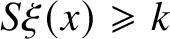
 $S\xi :\mathbb {Z}\to \{0,1,2,\dots \}\cup \{\infty \}$
is defined by
$S\xi :\mathbb {Z}\to \{0,1,2,\dots \}\cup \{\infty \}$
is defined by
 $$ \begin{align*} S\xi(x) := \begin{cases} m-1,&\text{if } x = \mathcal{T}_m(\gamma) \text{ or } \mathcal{H}_m(\gamma), \text{ for }\gamma \in\Gamma_k\xi \text{ and } k \geqslant m,\\ \infty,&\text{if } x \text{ is a record for } \xi. \end{cases} \end{align*} $$
For each
 $k\geqslant 1$
we say that x is a k-slot for
$k\geqslant 1$
we say that x is a k-slot for
 $\xi $
if
$\xi $
if
 $S\xi (x)\geqslant k$
.
$S\xi (x)\geqslant k$
.
Note that a record is a k-slot for all k, and an m-soliton contains a number
 $2m-2k$
of k-slots; see Figure 2.3. Because every
$2m-2k$
of k-slots; see Figure 2.3. Because every
 $\xi \in \mathcal {W}$
has infinitely many records, it also has infinitely many k-slots.
$\xi \in \mathcal {W}$
has infinitely many records, it also has infinitely many k-slots.
Slot configuration of a walk
 $\xi $
. Different colors correspond to different solitons; records are painted in black. For each site, the number of dots below it indicates its level in slots: k dots indicate a k-slot. (color online)
$\xi $
. Different colors correspond to different solitons; records are painted in black. For each site, the number of dots below it indicates its level in slots: k dots indicate a k-slot. (color online)
For
 $j\in \mathbb {Z}$
, the position of the record at level
$j\in \mathbb {Z}$
, the position of the record at level
 $-j$
will be called record j and denoted as
$-j$
will be called record j and denoted as
 $$ \begin{align*} r(\xi,j) := \min\{x\in\mathbb{Z}: \xi(x)=-j\}. \end{align*} $$
This is the leftmost site where the walk
 $\xi $
takes the value
$\xi $
takes the value
 $-j$
. If
$-j$
. If
 $\xi \in \mathcal {W}$
, we have
$\xi \in \mathcal {W}$
, we have
 $r(\xi,j) \in \mathbb {Z}$
well defined for all
$r(\xi,j) \in \mathbb {Z}$
well defined for all
 $j\in \mathbb {Z}$
. The site
$j\in \mathbb {Z}$
. The site
 $r(\xi, 0)$
will play a central role in the sequel. Note that
$r(\xi, 0)$
will play a central role in the sequel. Note that
 $T\xi (x) \leqslant \xi (x)$
by (2.2), so
$T\xi (x) \leqslant \xi (x)$
by (2.2), so
 $r(T\xi, j)\leqslant r(\xi, j)$
for all j.
$r(T\xi, j)\leqslant r(\xi, j)$
for all j.
We label all k-slots in increasing order:
 $\cdots <s_{k}(\xi, -1)<s_{k}(\xi, 0)<s_{k}(\xi, 1)<\cdots $
, where
$\cdots <s_{k}(\xi, -1)<s_{k}(\xi, 0)<s_{k}(\xi, 1)<\cdots $
, where
 $s_k(\xi,0):=r(\xi,0)$
. The set of k-slots of
$s_k(\xi,0):=r(\xi,0)$
. The set of k-slots of
 $\xi $
is denoted
$\xi $
is denoted
 $S_k\xi := \{s_k(\xi,i):{i\in \mathbb {Z}}\}$
. We then say that a k-soliton
$S_k\xi := \{s_k(\xi,i):{i\in \mathbb {Z}}\}$
. We then say that a k-soliton
 $\gamma $
is appended to the ith k-slot
$\gamma $
is appended to the ith k-slot
 $s_{k}(\xi, i)$
if
$s_{k}(\xi, i)$
if
 $\gamma \cap [s_k(\xi,i),s_k(\xi,i+1)-1]\ne \varnothing $
. Observe that if that is the case, we necessarily have
$\gamma \cap [s_k(\xi,i),s_k(\xi,i+1)-1]\ne \varnothing $
. Observe that if that is the case, we necessarily have
 $\gamma \subseteq [s_k(\xi,i)+1,s_k(\xi,i+1)-1]$
, as a consequence of Lemma 1.5 and the fact that k-slots can only be records or sites of solitons with larger size. It follows that each k-soliton in
$\gamma \subseteq [s_k(\xi,i)+1,s_k(\xi,i+1)-1]$
, as a consequence of Lemma 1.5 and the fact that k-slots can only be records or sites of solitons with larger size. It follows that each k-soliton in
 $\xi $
is appended to a unique k-slot. On the other hand, it is possible to have multiple k-solitons appended to a single k-slot. Finally, we let
$\xi $
is appended to a unique k-slot. On the other hand, it is possible to have multiple k-solitons appended to a single k-slot. Finally, we let
 $M_k\xi (i)$
be the number of k-solitons appended to the ith k-slot and call
$M_k\xi (i)$
be the number of k-solitons appended to the ith k-slot and call
 $M_{k}\xi =(M_{k}\xi (i))_{i\in \mathbb {Z}}$
the kth component of
$M_{k}\xi =(M_{k}\xi (i))_{i\in \mathbb {Z}}$
the kth component of
 $\xi $
. For instance, in the example of Figure 2.3, we have M
6
$\xi $
. For instance, in the example of Figure 2.3, we have M
6
 $\xi $
(0) = 1, M
5
$\xi $
(0) = 1, M
5
 $\xi $
(2) = 1, M
4
$\xi $
(2) = 1, M
4
 $\xi $
(2) = 1, M
1
$\xi $
(2) = 1, M
1
 $\xi $
(9) = 1, M
1
$\xi $
(9) = 1, M
1
 $\xi $
(18) = 1 and
$\xi $
(18) = 1 and
 $M_k\xi (i) = 0$
otherwise. See also Figure 2.4 for an illustration on how the solitons are nested inside each other via slots.
$M_k\xi (i) = 0$
otherwise. See also Figure 2.4 for an illustration on how the solitons are nested inside each other via slots.
An illustration of how the solitons are nested inside bigger solitons via slots, in the same sample configuration as in Figure 2.3. Solitons are represented by squares and slots by circles. For each
 $k \geqslant 1$
, each slot with index
$k \geqslant 1$
, each slot with index
 $m\geqslant k$
is a k-slot. We say it is the nth k-slot, where n is determined by counting how many k-slots appear before it in the depth-first order, and the counting starts from the 0th k-slot present at record 0.
$m\geqslant k$
is a k-slot. We say it is the nth k-slot, where n is determined by counting how many k-slots appear before it in the depth-first order, and the counting starts from the 0th k-slot present at record 0.

2.2 Reconstructing the configuration from the components
Here we prove Theorem 1.3. In this subsection only, we will work with a larger set of configurations than
 $\mathcal W$
. Let
$\mathcal W$
. Let
 $\mathcal W_{*}$
be the set of walks
$\mathcal W_{*}$
be the set of walks
 $\xi $
such that
$\xi $
such that
 $r(\xi, j)$
is well defined for all
$r(\xi, j)$
is well defined for all
 $j\in \mathbb {Z}$
. Even though
$j\in \mathbb {Z}$
. Even though
 $\mathcal W_{*}$
is not preserved by T, the Takahashi–Satsuma algorithm still applies, because all of the excursions of
$\mathcal W_{*}$
is not preserved by T, the Takahashi–Satsuma algorithm still applies, because all of the excursions of
 $\xi \in \mathcal W_{*}$
are finite. So the kth component
$\xi \in \mathcal W_{*}$
are finite. So the kth component
 $M_{k}$
described in Subsection 2.1 is also defined for all
$M_{k}$
described in Subsection 2.1 is also defined for all
 $\xi \in \mathcal W_{*}$
. On the other hand, because the slot decomposition
$\xi \in \mathcal W_{*}$
. On the other hand, because the slot decomposition
 $\xi \mapsto M\xi $
is insensitive to horizontal shifts, it is not possible to determine
$\xi \mapsto M\xi $
is insensitive to horizontal shifts, it is not possible to determine
 $\xi $
knowing
$\xi $
knowing
 $(M_k\xi )_{k\geqslant 1}$
. So we introduce
$(M_k\xi )_{k\geqslant 1}$
. So we introduce
 $$ \begin{align*} \skew5\widehat{\mathcal{W}}_{*}:= \{\xi\in\mathcal{W}_{*}: r(\xi,0)=0\}. \end{align*} $$
(As a side remark,
 $ \mathcal {W}_* $
is the set of simple walks
$ \mathcal {W}_* $
is the set of simple walks
 $ \xi $
such that
$ \xi $
such that
 $ \lim _{x\to -\infty } \xi (x)=+\infty $
and
$ \lim _{x\to -\infty } \xi (x)=+\infty $
and
 $ \liminf _{x\to +\infty } \xi (x) = -\infty $
. We can build a configuration
$ \liminf _{x\to +\infty } \xi (x) = -\infty $
. We can build a configuration
 $\xi \in \mathcal {W}_*$
with
$\xi \in \mathcal {W}_*$
with
 $ T\xi \not \in \mathcal {W}_* $
by appending a soliton of height
$ T\xi \not \in \mathcal {W}_* $
by appending a soliton of height
 $2^n$
between records
$2^n$
between records
 $ -n $
and
$ -n $
and
 $ -n+1 $
, so that
$ -n+1 $
, so that
 $ \liminf _{x\to -\infty } T\xi (x) = -\infty $
.)
$ \liminf _{x\to -\infty } T\xi (x) = -\infty $
.)
Note that, unlike the lift
 $\xi [\eta ]$
from
$\xi [\eta ]$
from
 $\mathcal {X}$
to
$\mathcal {X}$
to
 $\mathcal {W}$
, which was not unique, for
$\mathcal {W}$
, which was not unique, for
 $\eta $
in
$\eta $
in
 $ \skew8\widehat{\mathcal {X}} $
there is a unique lift
$ \skew8\widehat{\mathcal {X}} $
there is a unique lift
 $\xi [\eta ]$
that is in
$\xi [\eta ]$
that is in
 $\skew5\widehat {\mathcal {W}}_{*}$
. We denote this unique lift by
$\skew5\widehat {\mathcal {W}}_{*}$
. We denote this unique lift by
 $\xi ^{\circ }[\eta ]$
. So the maps
$\xi ^{\circ }[\eta ]$
. So the maps
 $ \eta \mapsto M_k \eta $
as seen in Theorem 1.3 are given by
$ \eta \mapsto M_k \eta $
as seen in Theorem 1.3 are given by
 $M_k\eta = M_k\xi ^{\circ }[\eta ]$
. But to remain consistent with the previous subsections, we continue to work with
$M_k\eta = M_k\xi ^{\circ }[\eta ]$
. But to remain consistent with the previous subsections, we continue to work with
 $\xi $
instead of
$\xi $
instead of
 $\eta $
.
$\eta $
.
Denote by M the map
 $\xi \mapsto M\xi :=(M_k\xi )_{k\geqslant 1}$
. We now show that
$\xi \mapsto M\xi :=(M_k\xi )_{k\geqslant 1}$
. We now show that
 $M: \skew5\widehat {\mathcal {W}}_{*}\to \mathcal M$
is invertible.
$M: \skew5\widehat {\mathcal {W}}_{*}\to \mathcal M$
is invertible.
The height of the excursion between record j and record
 $j+1$
, denoted as
$j+1$
, denoted as
 $m(j)$
, is defined as
$m(j)$
, is defined as
 $0$
if the excursion is empty or as the largest k such that a k-soliton is contained in the excursion. Denote also
$0$
if the excursion is empty or as the largest k such that a k-soliton is contained in the excursion. Denote also
 $i_k(j)$
the label of the k-slot located at record j. Because k-slots can only be created by solitons of larger sizes, we note that
$i_k(j)$
the label of the k-slot located at record j. Because k-slots can only be created by solitons of larger sizes, we note that
 $$ \begin{align*} m(j) &= \min\{k\geqslant 0: M_{k'}\xi(i_{k'}(j))=0 \text{ for all }k'>k\} \in \{0,1,2,\dots\}. \end{align*} $$
Both
 $m(j)$
and
$m(j)$
and
 $i_k(j)$
depend on
$i_k(j)$
depend on
 $\xi $
but we omit it in the notation. Denote the slot decomposition
$\xi $
but we omit it in the notation. Denote the slot decomposition
 $M\xi $
of
$M\xi $
of
 $\xi $
by
$\xi $
by
 $\zeta $
; that is,
$\zeta $
; that is,
 $$ \begin{align*} \zeta = (\zeta_k)_k = M \xi. \end{align*} $$
Note that each
 $\xi \in \mathcal {W}_{*}$
and
$\xi \in \mathcal {W}_{*}$
and
 $j\in \mathbb {Z}$
,
$j\in \mathbb {Z}$
,
 $i_k(j)=r(\xi,j)$
for all
$i_k(j)=r(\xi,j)$
for all
 $k\geqslant \max \{m(0), \dots, m(j)\}$
. Because
$k\geqslant \max \{m(0), \dots, m(j)\}$
. Because
 $m(j)$
is finite, we have that
$m(j)$
is finite, we have that
 $$ \begin{align} \text{ for each } i\in\mathbb{Z},\ \zeta_k(i) = 0 \text{ for all large } k. \end{align} $$
Namely,
 $\zeta \in \mathcal M$
. Conversely, suppose that
$\zeta \in \mathcal M$
. Conversely, suppose that
 $\zeta = (\zeta _k)_{k\geqslant 1} \in \mathcal M$
, so, in, particular
$\zeta = (\zeta _k)_{k\geqslant 1} \in \mathcal M$
, so, in, particular
 $\zeta $
satisfies (2.3). We first give an algorithm to reconstruct the excursion of
$\zeta $
satisfies (2.3). We first give an algorithm to reconstruct the excursion of
 $\xi $
between records 0 and 1. To that end, we introduce the following notation: denote the number of k-slots in the excursion
$\xi $
between records 0 and 1. To that end, we introduce the following notation: denote the number of k-slots in the excursion
 $\varepsilon $
between successive records
$\varepsilon $
between successive records
 $y_1<y_2$
by
$y_1<y_2$
by
 $$ \begin{align} n_k(\varepsilon) := 1 + |S_k \xi \cap \{y_1+1,\dots, y_2-1\}|, \end{align} $$
where the term
 $1$
refers to the record
$1$
refers to the record
 $y_1$
preceding
$y_1$
preceding
 $\varepsilon $
and the second term counts the number of k-slots belonging to m-solitons of
$\varepsilon $
and the second term counts the number of k-slots belonging to m-solitons of
 $\varepsilon $
with
$\varepsilon $
with
 $m>k$
. Here is the algorithm:
$m>k$
. Here is the algorithm:

Note that m is well defined by (2.3). In case
 $m=0$
, the algorithm produces an empty configuration. Let us also note that when inserting solitons in the above algorithm, there is only one way to do it consistently with the soliton decomposition: if a soliton is inserted to the right of the site x with
$m=0$
, the algorithm produces an empty configuration. Let us also note that when inserting solitons in the above algorithm, there is only one way to do it consistently with the soliton decomposition: if a soliton is inserted to the right of the site x with
 $\eta (x)=0$
, then it has its head on the left and tail on the right (i.e.,
$\eta (x)=0$
, then it has its head on the left and tail on the right (i.e.,
 $11\cdots 100\cdots 0$
); otherwise, it is inserted with its tail on the left and head on the right (i.e.,
$11\cdots 100\cdots 0$
); otherwise, it is inserted with its tail on the left and head on the right (i.e.,
 $00\cdots 011\cdots 1$
). The procedure is illustrated in Figure 2.5. Call
$00\cdots 011\cdots 1$
). The procedure is illustrated in Figure 2.5. Call
 $\varepsilon ^0$
the excursion between record
$\varepsilon ^0$
the excursion between record
 $0$
and record
$0$
and record
 $1$
obtained from
$1$
obtained from
 $ \zeta $
as just described. Construct
$ \zeta $
as just described. Construct
 $\varepsilon ^1$
, the excursion between records 1 and 2, using the same algorithm but with the data
$\varepsilon ^1$
, the excursion between records 1 and 2, using the same algorithm but with the data
 $\zeta ^1 = (\zeta ^1_k)_{k\geqslant 1}$
, where each component is given by
$\zeta ^1 = (\zeta ^1_k)_{k\geqslant 1}$
, where each component is given by
 $$ \begin{align*} \zeta^1_k = \big( \zeta_k(n_k+i) \big)_{i \geqslant 0}, \end{align*} $$
which consists of the entries of
 $\zeta $
with nonnegative indices i not used in the reconstruction of
$\zeta $
with nonnegative indices i not used in the reconstruction of
 $\varepsilon ^0$
. Note that
$\varepsilon ^0$
. Note that
 $\zeta ^1$
also satisfies (2.3). Iterate this procedure to construct an infinite sequence of excursions
$\zeta ^1$
also satisfies (2.3). Iterate this procedure to construct an infinite sequence of excursions
 $(\varepsilon ^j)_{j=0,1,2,\dots }$
. See Figure 2.7.
$(\varepsilon ^j)_{j=0,1,2,\dots }$
. See Figure 2.7.
Reconstruction algorithm for a single excursion. This example is obtained using the field
 $\zeta $
shown in Figure 2.6.
$\zeta $
shown in Figure 2.6.

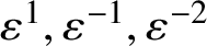
Reconstruction of
 $\xi $
from
$\xi $
from
 $\zeta $
. In the lower part we show records
$\zeta $
. In the lower part we show records
 $-2$
to
$-2$
to
 $2$
in boldface and the excursions between them. Above we show the parts of the field
$2$
in boldface and the excursions between them. Above we show the parts of the field
 $\zeta $
used in the reconstruction of
$\zeta $
used in the reconstruction of
 $\varepsilon ^{-2},\varepsilon ^{-1},\varepsilon ^{0},\varepsilon ^{1}$
. Reconstruction of
$\varepsilon ^{-2},\varepsilon ^{-1},\varepsilon ^{0},\varepsilon ^{1}$
. Reconstruction of
 $\varepsilon ^0$
was shown in Figure 2.5 and
$\varepsilon ^0$
was shown in Figure 2.5 and
 $\varepsilon ^{1},\varepsilon ^{-1},\varepsilon ^{-2}$
is shown in Figure 2.7.
$\varepsilon ^{1},\varepsilon ^{-1},\varepsilon ^{-2}$
is shown in Figure 2.7.
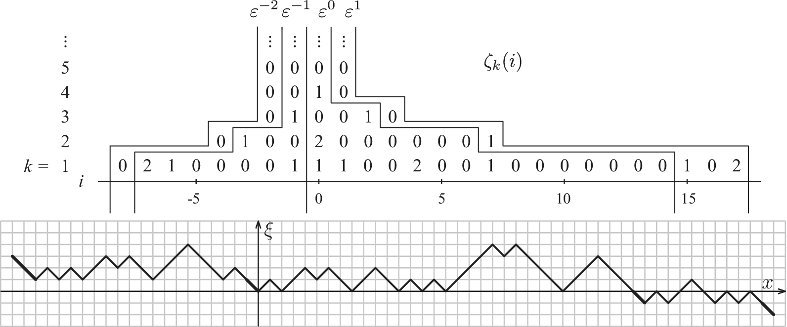
Reconstruction algorithm for other excursions. The procedure is the same as in Figure 2.5 but all of the intermediate steps are omitted.
To reconstruct the configuration to the left of record
 $0$
– that is, to obtain the excursions
$0$
– that is, to obtain the excursions
 $\varepsilon ^j$
with negative j – we use an analogous algorithm that uses the entries of
$\varepsilon ^j$
with negative j – we use an analogous algorithm that uses the entries of
 $\zeta $
with i-indices starting at
$\zeta $
with i-indices starting at
 $-1$
and moving left instead of starting at
$-1$
and moving left instead of starting at
 $0$
and moving right. First take
$0$
and moving right. First take
 $\zeta ^{-1} = (\zeta ^{-1}_k)_{k \geqslant 1}$
where each component is given by
$\zeta ^{-1} = (\zeta ^{-1}_k)_{k \geqslant 1}$
where each component is given by
 $\zeta ^{-1}_k = \big ( \zeta _k(i) \big )_{i < 0}$
and use
$\zeta ^{-1}_k = \big ( \zeta _k(i) \big )_{i < 0}$
and use
 $\zeta ^{-1}$
to construct
$\zeta ^{-1}$
to construct
 $\varepsilon ^{-1}$
. Then define
$\varepsilon ^{-1}$
. Then define
 $\zeta ^{-2} = (\zeta ^{-2}_k)_{k \geqslant 1}$
where each component is given by
$\zeta ^{-2} = (\zeta ^{-2}_k)_{k \geqslant 1}$
where each component is given by
 $\zeta ^{-2}_k = \big ( \zeta _k(i-n_k) \big )_{i < 0}$
and use it to construct
$\zeta ^{-2}_k = \big ( \zeta _k(i-n_k) \big )_{i < 0}$
and use it to construct
 $\varepsilon ^{-2}$
. Iterate this procedure to construct an infinite sequence of excursions
$\varepsilon ^{-2}$
. Iterate this procedure to construct an infinite sequence of excursions
 $(\varepsilon ^j)_{j=-1,-2,\dots }$
.
$(\varepsilon ^j)_{j=-1,-2,\dots }$
.
Put record
 $0$
at the origin and concatenate the excursions with one record between each pair of consecutive excursions. This yields a walk denoted as
$0$
at the origin and concatenate the excursions with one record between each pair of consecutive excursions. This yields a walk denoted as
 $\xi ^*$
, shown in Figure 2.6. Note that in
$\xi ^*$
, shown in Figure 2.6. Note that in
 $\xi ^{*}$
, all excursions are finite and therefore
$\xi ^{*}$
, all excursions are finite and therefore
 $r(\xi, j)$
is finite for all
$r(\xi, j)$
is finite for all
 $j\in \mathbb {Z}$
. Namely,
$j\in \mathbb {Z}$
. Namely,
 $\xi ^{*}\in \skew5\widehat {\mathcal {W}}_{*}$
.
$\xi ^{*}\in \skew5\widehat {\mathcal {W}}_{*}$
.
Call
 $M^{-1}:\zeta \mapsto \xi ^*$
the resulting transformation. We claim that
$M^{-1}:\zeta \mapsto \xi ^*$
the resulting transformation. We claim that
 $M^{-1}$
is the inverse map of M; that is,
$M^{-1}$
is the inverse map of M; that is,
 $M^{-1} M\xi = \xi $
for
$M^{-1} M\xi = \xi $
for
 $\xi \in \skew5\widehat {\mathcal {W}}_{*}$
and
$\xi \in \skew5\widehat {\mathcal {W}}_{*}$
and
 $MM^{-1}\zeta =\zeta $
for
$MM^{-1}\zeta =\zeta $
for
 $\zeta \in \mathcal M$
. The second identity follows from the fact that
$\zeta \in \mathcal M$
. The second identity follows from the fact that
 $M_{k}\xi ^{*}=\zeta _{k}$
for each k. Now let
$M_{k}\xi ^{*}=\zeta _{k}$
for each k. Now let
 $\varepsilon $
be an excursion of
$\varepsilon $
be an excursion of
 $ \xi $
. For
$ \xi $
. For
 $k\geqslant 0$
, denote by
$k\geqslant 0$
, denote by
 $\varepsilon _{[k]}$
the ball configuration obtained by removing the boxes belonging to an
$\varepsilon _{[k]}$
the ball configuration obtained by removing the boxes belonging to an
 $\ell $
-soliton with
$\ell $
-soliton with
 $\ell \leqslant k$
. Then
$\ell \leqslant k$
. Then
 $\varepsilon _{[0]}=\varepsilon $
and
$\varepsilon _{[0]}=\varepsilon $
and
 $\varepsilon _{[k]}$
is the empty excursion for k sufficiently large. Now observe from the previous definitions that
$\varepsilon _{[k]}$
is the empty excursion for k sufficiently large. Now observe from the previous definitions that
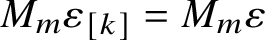 $M_m\varepsilon _{[k]}=M_m \varepsilon $
for all
$M_m\varepsilon _{[k]}=M_m \varepsilon $
for all
 $m>k$
, because m-slots are only created by solitons of sizes larger than m. So the reconstruction algorithm correctly finds
$m>k$
, because m-slots are only created by solitons of sizes larger than m. So the reconstruction algorithm correctly finds
 $\varepsilon _{[k]}$
from
$\varepsilon _{[k]}$
from
 $M_{k}\varepsilon $
and
$M_{k}\varepsilon $
and
 $\varepsilon _{[k+1]}$
and hence it correctly finds
$\varepsilon _{[k+1]}$
and hence it correctly finds
 $\varepsilon $
.
$\varepsilon $
.
This shows that
 $M: \skew5\widehat {\mathcal {W}}_{*}\to \mathcal M$
is invertible, and so is its restriction to a subset
$M: \skew5\widehat {\mathcal {W}}_{*}\to \mathcal M$
is invertible, and so is its restriction to a subset
 $M: \skew5\widehat {\mathcal {W}}\to M(\skew5\widehat {\mathcal {W}})\subseteq \mathcal M$
, where
$M: \skew5\widehat {\mathcal {W}}\to M(\skew5\widehat {\mathcal {W}})\subseteq \mathcal M$
, where
 $\skew5\widehat {\mathcal {W}}:=\{\xi [\eta ]\in \skew5\widehat {\mathcal {W}}_{*}: \eta \in \skew8\widehat{\mathcal {X}}\}$
. This proves Theorem 1.3.
$\skew5\widehat {\mathcal {W}}:=\{\xi [\eta ]\in \skew5\widehat {\mathcal {W}}_{*}: \eta \in \skew8\widehat{\mathcal {X}}\}$
. This proves Theorem 1.3.
Let us also point out that the image set
 $M(\skew5\widehat {\mathcal {W}})$
is not simple to characterise. However, as we will see below, if we sample
$M(\skew5\widehat {\mathcal {W}})$
is not simple to characterise. However, as we will see below, if we sample
 $\zeta $
with an appropriate measure, the resulting (random) element
$\zeta $
with an appropriate measure, the resulting (random) element
 $M^{-1}\zeta $
does belong a.s. to
$M^{-1}\zeta $
does belong a.s. to
 $\skew5\widehat {\mathcal {W}}$
.
$\skew5\widehat {\mathcal {W}}$
.
3 Evolution of components
Here we prove a stronger version of Theorem 1.4. Recall that we can track a tagged soliton
 $\gamma $
after t iterations of T by (1.4). In order to describe how the BBS dynamics act on the components, we introduce the flows of solitons as follows. First, let
$\gamma $
after t iterations of T by (1.4). In order to describe how the BBS dynamics act on the components, we introduce the flows of solitons as follows. First, let
 $$ \begin{align*} J^t_m \xi := \# \big\{ \gamma\in\Gamma_m\xi : \gamma\subseteq(-\infty,r(\xi,0))\text{ and } \gamma^t \subseteq[r(T^t\xi,0),\infty)\big\}. \end{align*} $$
In words,
 $J^{t}_{m}\xi $
counts the number of m-solitons that were to the left of record
$J^{t}_{m}\xi $
counts the number of m-solitons that were to the left of record
 $0$
initially and are found to be on the right of record
$0$
initially and are found to be on the right of record
 $0$
at time t. We say that such solitons cross record
$0$
at time t. We say that such solitons cross record
 $0$
. Note that this is not the same as ‘crossing the origin’ because record
$0$
. Note that this is not the same as ‘crossing the origin’ because record
 $ 0 $
is itself moving left.
$ 0 $
is itself moving left.
Note that
 $ J^1_m \xi =0 $
for all large
$ J^1_m \xi =0 $
for all large
 $ m $
. Indeed, using Proposition 1.3 one can see that no more than
$ m $
. Indeed, using Proposition 1.3 one can see that no more than
 $ r(\xi,0)-r(T\xi,0) $
solitons can cross record
$ r(\xi,0)-r(T\xi,0) $
solitons can cross record
 $0$
at time
$0$
at time
 $1$
, so
$1$
, so
 $ \sum _m J^1_m \xi < \infty $
. By the same argument,
$ \sum _m J^1_m \xi < \infty $
. By the same argument,
 $ \sum _m J^2_m \xi < \infty $
, and so on.
$ \sum _m J^2_m \xi < \infty $
, and so on.
We now define an observable
 $o^t_k(\xi )$
that counts the flow of k-slots through record
$o^t_k(\xi )$
that counts the flow of k-slots through record
 $0$
after t iterations of T. Because each m-soliton crossing record
$0$
after t iterations of T. Because each m-soliton crossing record
 $0$
from left to right carries
$0$
from left to right carries
 $2(m-k) \ k$
-slots, we define
$2(m-k) \ k$
-slots, we define
 $$ \begin{align} o^t_k(\xi) := \sum_{m>k} 2(m-k) J^t_m \xi<\infty. \end{align} $$
Using the observable
 $o^t_k(\xi )$
, we define the tagged
$o^t_k(\xi )$
, we define the tagged
 $0$
th k-slot at time t by
$0$
th k-slot at time t by
 $$ \begin{align*} s^t_k(\xi,0) &:= s_k(T^t\xi,o^t_k(\xi)), \end{align*} $$
which is the position of the
 $o_k^t$
th k-slot counting from record
$o_k^t$
th k-slot counting from record
 $0$
of
$0$
of
 $T^t\xi $
. More generally, the tagged ith k-slot at time t is defined as
$T^t\xi $
. More generally, the tagged ith k-slot at time t is defined as
 $$ \begin{align*} s^t_k(\xi,i) &:= s_k(T^t\xi,o^t_k(\xi)+i). \end{align*} $$
We now state one of the central results of this article. In some sense, it shows that the action of
 $ T $
on the component configuration
$ T $
on the component configuration
 $ (M_k \xi )_{k \in \mathbb {N}} $
has a simple form, analogous to a Jordan form or upper triangular form for a linear map. The kth component is shifted by k units, plus possibly a number resulting from the re-indexing of k-slots caused by larger solitons crossing record
$ (M_k \xi )_{k \in \mathbb {N}} $
has a simple form, analogous to a Jordan form or upper triangular form for a linear map. The kth component is shifted by k units, plus possibly a number resulting from the re-indexing of k-slots caused by larger solitons crossing record
 $ 0 $
.
$ 0 $
.
Theorem 3.1. Let
 $\xi \in \mathcal {W}$
and
$\xi \in \mathcal {W}$
and
 $t\in \{1,2, 3, \dots \}$
. Then, for any k-soliton
$t\in \{1,2, 3, \dots \}$
. Then, for any k-soliton
 $\gamma $
of
$\gamma $
of
 $\xi $
,
$\xi $
,
 $$ \begin{align*} \# \Big\{ {i\in\mathbb{Z}} : \gamma \subseteq \big( -\infty,s_k(\xi,i) \big) \text{ and } \gamma^t \subseteq \big[s^t_k(\xi,i),\infty\big) \Big\} = kt; \end{align*} $$
that is, between times
 $0$
and t a tagged k-soliton moves
$0$
and t a tagged k-soliton moves
 $kt$
units to the right in terms of tagged k-slots or, equivalently, the right-to-left flow of tagged k-slots through a tagged k-soliton is exactly
$kt$
units to the right in terms of tagged k-slots or, equivalently, the right-to-left flow of tagged k-slots through a tagged k-soliton is exactly
 $kt$
. For each
$kt$
. For each
 $k\in \mathbb {N}$
, the k-soliton component of
$k\in \mathbb {N}$
, the k-soliton component of
 $T^t\xi $
is a shift of the k-soliton component of
$T^t\xi $
is a shift of the k-soliton component of
 $\xi $
:
$\xi $
:
 $$ \begin{align*} M_k T^t \xi(i) = M_k\xi\big(i - o^t_k(\xi)-kt\big), \end{align*} $$
where
 $o^{t}_{k}(\xi )$
is defined in (3.1). Moreover, the offset
$o^{t}_{k}(\xi )$
is defined in (3.1). Moreover, the offset
 $o_k^t(\xi )$
is determined by
$o_k^t(\xi )$
is determined by
 $(M_m \xi )_{m>k}$
, so that
$(M_m \xi )_{m>k}$
, so that
 $M_{k}T^{t}\xi $
is a function of
$M_{k}T^{t}\xi $
is a function of
 $(M_m \xi )_{m \geqslant k}$
.
$(M_m \xi )_{m \geqslant k}$
.
Another way to interpret the theorem is based on the notion of k-bearer, which we introduce now. Let
 $\pi \in S_k\xi \subseteq \mathbb {Z}$
. Then
$\pi \in S_k\xi \subseteq \mathbb {Z}$
. Then
 $\pi = s_k(\xi,j)$
for some j, and we define the corresponding k-bearer at time t to be
$\pi = s_k(\xi,j)$
for some j, and we define the corresponding k-bearer at time t to be
 $$ \begin{align} \pi^{k,t} := s_k \big( T^t\xi,o^t_k(\xi)+kt+j \big). \end{align} $$
An immediate consequence of Theorem 3.1 is as follows: a k-soliton
 $\gamma $
is appended to the k-slot located at
$\gamma $
is appended to the k-slot located at
 $\pi =s_k(\xi,j)$
if and only if
$\pi =s_k(\xi,j)$
if and only if
 $\gamma ^{t}$
is appended to the k-slot located at
$\gamma ^{t}$
is appended to the k-slot located at
 $\pi ^{k, t}$
. In particular, because the definition of a tagged soliton depends only on
$\pi ^{k, t}$
. In particular, because the definition of a tagged soliton depends only on
 $\eta [\xi ]$
according to Proposition 1.3, this implies that
$\eta [\xi ]$
according to Proposition 1.3, this implies that
 $\pi ^{k,t}$
also only depends on
$\pi ^{k,t}$
also only depends on
 $\eta [\xi ]$
. We note that the difference between the tagged slots introduced before and bearers introduced just now is the factor of
$\eta [\xi ]$
. We note that the difference between the tagged slots introduced before and bearers introduced just now is the factor of
 $kt$
related to the motion of k-solitons. So a tagged k-soliton crosses k tagged k-slots per unit time, whereas it does not cross k-bearers (in fact, it just follows one of them). As a side remark, the notion of k-bearer allows us to define the soliton speed
$kt$
related to the motion of k-solitons. So a tagged k-soliton crosses k tagged k-slots per unit time, whereas it does not cross k-bearers (in fact, it just follows one of them). As a side remark, the notion of k-bearer allows us to define the soliton speed
 $v_{k}$
even if
$v_{k}$
even if
 $\rho _{k}=0$
by replacing
$\rho _{k}=0$
by replacing
 $x(\gamma ^{t})$
with
$x(\gamma ^{t})$
with
 $\pi ^{k, t}$
in (1.9).
$\pi ^{k, t}$
in (1.9).
Proof of Theorem 3.1. We start by showing how the second statement follows from the first one. Because every k-soliton crosses exactly k tagged k-slots at each step, the number of k-slots between any pair of tagged k-solitons is conserved by T. Hence, the kth component as seen from the tagged
 $0$
th k-slot just shifts
$0$
th k-slot just shifts
 $k \ k$
-slots per unit time, and the term
$k \ k$
-slots per unit time, and the term
 $o^t_k(\xi )$
accounts for the relabeling of k-slots caused by bigger solitons crossing record 0.
$o^t_k(\xi )$
accounts for the relabeling of k-slots caused by bigger solitons crossing record 0.
For the proof of the first statement, it suffices to consider the case
 $t=1$
. Let us first assume that there is only a finite number of balls in
$t=1$
. Let us first assume that there is only a finite number of balls in
 $\xi [\eta ]$
. Without loss of generality, we can also assume
$\xi [\eta ]$
. Without loss of generality, we can also assume
 $r(\xi, 0)=0$
. For
$r(\xi, 0)=0$
. For
 $x\in \mathbb {Z}_{+}$
, let us define
$x\in \mathbb {Z}_{+}$
, let us define
 $D_{k}(\xi, x)=\# S_{k}T\xi \cap [0, x] - \# S_{k}\xi \cap [0, x]$
, namely, the change in the number of k-slots found in
$D_{k}(\xi, x)=\# S_{k}T\xi \cap [0, x] - \# S_{k}\xi \cap [0, x]$
, namely, the change in the number of k-slots found in
 $[0, x]$
after one iteration of T. Let us recall the notation
$[0, x]$
after one iteration of T. Let us recall the notation
 $\mathcal {H}_{i}(\gamma )$
, which stands for the ith site of the head of a soliton
$\mathcal {H}_{i}(\gamma )$
, which stands for the ith site of the head of a soliton
 $\gamma $
. We introduce the set
$\gamma $
. We introduce the set
 $\mathcal D_{k}(\xi, x)=\{z\in [0, x]: \exists \,\gamma \text { s.t. } z=\mathcal {H}_{i}(\gamma ), 1\leqslant i\leqslant k \text { and } \mathcal {T}_{i}(\gamma ^{1})>x\}$
. Let us observe that if such a soliton
$\mathcal D_{k}(\xi, x)=\{z\in [0, x]: \exists \,\gamma \text { s.t. } z=\mathcal {H}_{i}(\gamma ), 1\leqslant i\leqslant k \text { and } \mathcal {T}_{i}(\gamma ^{1})>x\}$
. Let us observe that if such a soliton
 $\gamma $
exists, then necessarily
$\gamma $
exists, then necessarily
 $x(\gamma ^{1})> x(\gamma )$
; otherwise,
$x(\gamma ^{1})> x(\gamma )$
; otherwise,
 $\gamma $
merely swaps its head and tail, and we will have
$\gamma $
merely swaps its head and tail, and we will have
 $\mathcal {T}_{i}(\gamma ^{1})=\mathcal {H}_{i}(\gamma )$
in that case. Therefore,
$\mathcal {T}_{i}(\gamma ^{1})=\mathcal {H}_{i}(\gamma )$
in that case. Therefore,
 $\#\mathcal D_{k}(\xi, x)$
counts the number of slots in
$\#\mathcal D_{k}(\xi, x)$
counts the number of slots in
 $[0, x]$
that have order
$[0, x]$
that have order
 $<k$
and belong to the heads of solitons that move to the right of x after one iteration. See Figure 3.1 for an example. We claim that for all
$<k$
and belong to the heads of solitons that move to the right of x after one iteration. See Figure 3.1 for an example. We claim that for all
 $x\in \mathbb {Z}_{+}$
and all
$x\in \mathbb {Z}_{+}$
and all
 $k\geqslant 1$
,
$k\geqslant 1$
,
 $$ \begin{align} D_{k}(\xi, x)=\# \mathcal D_{k}(\xi, x). \end{align} $$
To prove this, let us first suppose that
 $\eta $
consists of one soliton, say, at the sites
$\eta $
consists of one soliton, say, at the sites
 $[0, 2m)$
. Then the slot configuration
$[0, 2m)$
. Then the slot configuration
 $ST\xi $
is obtained from
$ST\xi $
is obtained from
 $S\xi $
by swapping the labels of the sites in
$S\xi $
by swapping the labels of the sites in
 $[0, m-1]$
with those in
$[0, m-1]$
with those in
 $[2m, 3m-1]$
. One readily checks that in this case
$[2m, 3m-1]$
. One readily checks that in this case
 $D_{k}(\xi, x)$
is tent shaped: linear with slope
$D_{k}(\xi, x)$
is tent shaped: linear with slope
 $1$
on
$1$
on
 $[0, k\wedge m-1]$
, constant on
$[0, k\wedge m-1]$
, constant on
 $[k\wedge m-1, 2m]$
and null on
$[k\wedge m-1, 2m]$
and null on
 $[2m+m\wedge k, \infty )$
. This can be similarly checked for
$[2m+m\wedge k, \infty )$
. This can be similarly checked for
 $\mathcal D_{k}(\xi, x)$
and the claimed identity holds in this case.
$\mathcal D_{k}(\xi, x)$
and the claimed identity holds in this case.
We depict
 $T\xi $
below
$T\xi $
below
 $\xi $
. This example illustrates the various situations discussed in the proof of Theorem 3.1. For instance, the
$\xi $
. This example illustrates the various situations discussed in the proof of Theorem 3.1. For instance, the
 $5$
-soliton (in pink) stays put and is nested in the
$5$
-soliton (in pink) stays put and is nested in the
 $6$
-soliton (in blue). The displacement of the 6-soliton brings five ‘new’ 5-slots to the left of the 5-soliton. (color online)
$6$
-soliton (in blue). The displacement of the 6-soliton brings five ‘new’ 5-slots to the left of the 5-soliton. (color online)
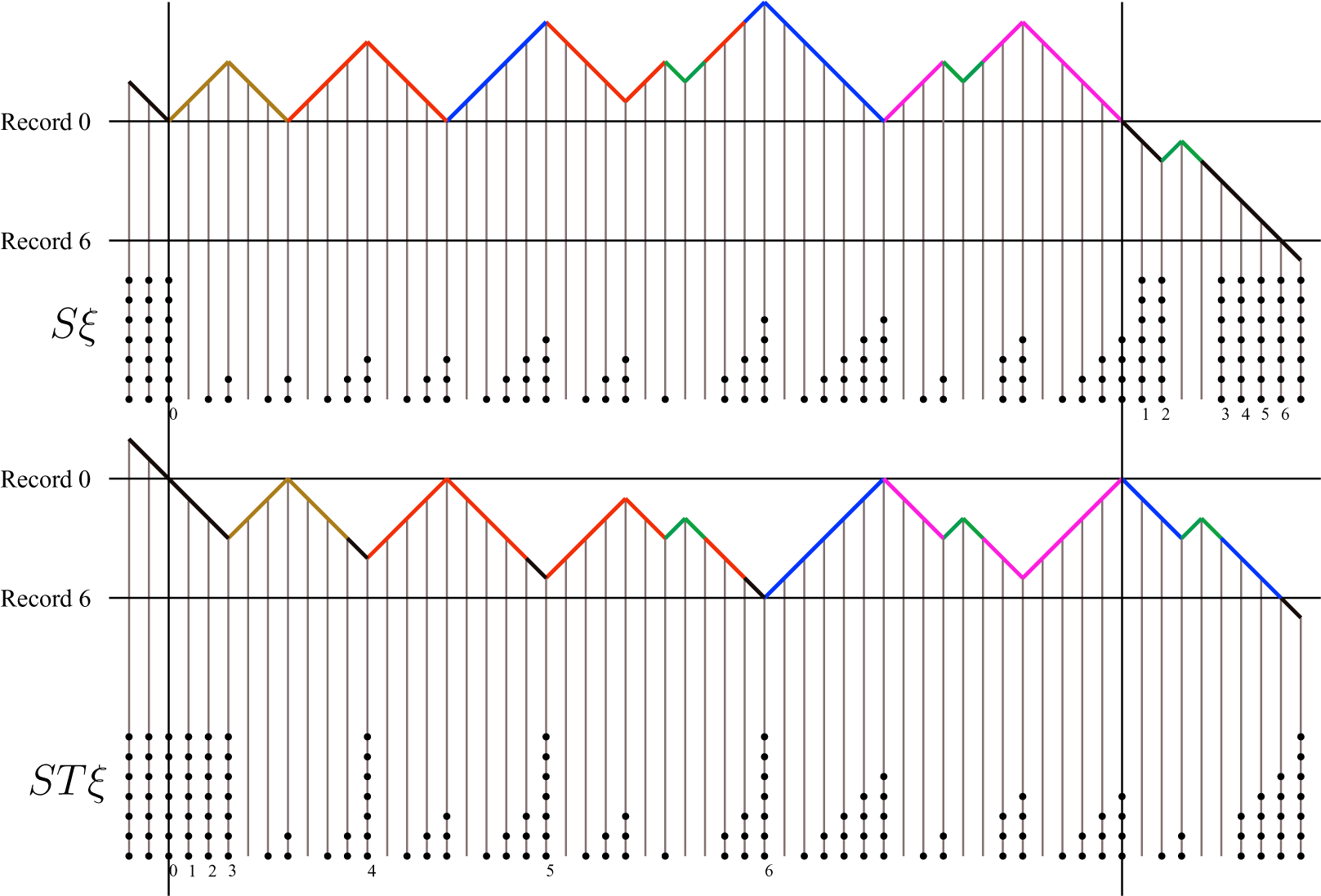
For a general configuration
 $\xi $
, the sites in
$\xi $
, the sites in
 $\mathcal D_{k}(\xi, x)$
do not necessarily become records in
$\mathcal D_{k}(\xi, x)$
do not necessarily become records in
 $T\xi $
, because they can be claimed by other solitons. However, we will see that even if this happens, it will only affect where the ‘new’ k-slots are located but not the quantity
$T\xi $
, because they can be claimed by other solitons. However, we will see that even if this happens, it will only affect where the ‘new’ k-slots are located but not the quantity
 $D_{k}(\xi, x)$
. Proceeding with the proof of (3.3), let us suppose that it holds for configurations with up to
$D_{k}(\xi, x)$
. Proceeding with the proof of (3.3), let us suppose that it holds for configurations with up to
 $p\geqslant 1$
solitons and let
$p\geqslant 1$
solitons and let
 $\xi [\eta ]$
be a configuration with
$\xi [\eta ]$
be a configuration with
 $p+1$
solitons. Let
$p+1$
solitons. Let
 $m\geqslant 1$
be the smallest size of the solitons in
$m\geqslant 1$
be the smallest size of the solitons in
 $\xi $
and let
$\xi $
and let
 $\gamma $
be its leftmost m-soliton. We note that
$\gamma $
be its leftmost m-soliton. We note that
 $\mathcal {H}(\gamma )$
and
$\mathcal {H}(\gamma )$
and
 $\mathcal {T}(\gamma )$
is back-to-back in
$\mathcal {T}(\gamma )$
is back-to-back in
 $\xi $
(i.e., no other solitons lodged inside
$\xi $
(i.e., no other solitons lodged inside
 $\gamma $
) as a consequence of Lemma 1.5. Then we can write
$\gamma $
) as a consequence of Lemma 1.5. Then we can write
 $I(\gamma )=\mathcal {H}(\gamma )\cup \mathcal {T}(\gamma )=[a, a+2m)$
with
$I(\gamma )=\mathcal {H}(\gamma )\cup \mathcal {T}(\gamma )=[a, a+2m)$
with
 $a=x(\gamma )$
. Let us introduce
$a=x(\gamma )$
. Let us introduce
 $\tilde \xi (x)=\xi (x+2m)$
for all
$\tilde \xi (x)=\xi (x+2m)$
for all
 $x\geqslant a$
and
$x\geqslant a$
and
 $\tilde \xi (x)=\xi (x)$
otherwise. Namely,
$\tilde \xi (x)=\xi (x)$
otherwise. Namely,
 $\tilde \xi $
is the configuration obtained by removing
$\tilde \xi $
is the configuration obtained by removing
 $\gamma $
. By noting that the operator T consists in flipping portions of
$\gamma $
. By noting that the operator T consists in flipping portions of
 $\xi $
between consecutive records, we deduce that
$\xi $
between consecutive records, we deduce that
 $$ \begin{align*} T\xi(x)=T\tilde\xi(a-1)+\sum_{a\leqslant y\leqslant x}(1-2\eta(y)), \quad \text{ if } x\in [a, a+2m), \end{align*} $$
and
 $T\xi (x)=T\tilde \xi (x-2m)$
if
$T\xi (x)=T\tilde \xi (x-2m)$
if
 $x\geqslant a+2m$
, and
$x\geqslant a+2m$
, and
 $T\xi (x)=T\tilde \xi (x)$
otherwise. In words,
$T\xi (x)=T\tilde \xi (x)$
otherwise. In words,
 $T\xi $
is obtained by inserting a ‘flipped’ version of
$T\xi $
is obtained by inserting a ‘flipped’ version of
 $\gamma $
into
$\gamma $
into
 $T\tilde \xi $
at site a.
$T\tilde \xi $
at site a.
To check (3.3), let us first note that if
 $x(\gamma ^{1})=x(\gamma )$
, then
$x(\gamma ^{1})=x(\gamma )$
, then
 $ST\xi $
is simply obtained by inserting the slot configurations of the sites in
$ST\xi $
is simply obtained by inserting the slot configurations of the sites in
 $\gamma ^{1}$
into
$\gamma ^{1}$
into
 $ST\tilde \xi $
, so that
$ST\tilde \xi $
, so that
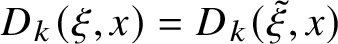 $D_{k}(\xi, x)=D_{k}(\tilde \xi, x)$
for
$D_{k}(\xi, x)=D_{k}(\tilde \xi, x)$
for
 $x<a$
,
$x<a$
,
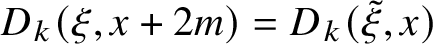 $D_{k}(\xi, x+2m)=D_{k}(\tilde \xi, x)$
for
$D_{k}(\xi, x+2m)=D_{k}(\tilde \xi, x)$
for
 $x\geqslant a$
and
$x\geqslant a$
and
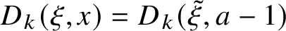 $D_{k}(\xi, x)=D_{k}(\tilde \xi, a-1)$
for
$D_{k}(\xi, x)=D_{k}(\tilde \xi, a-1)$
for
 $a\leqslant x< a+2m$
. In other words, putting
$a\leqslant x< a+2m$
. In other words, putting
 $\gamma $
back does not modify
$\gamma $
back does not modify
 $D_{k}(\xi, x)$
in real terms. A similar relationship holds between
$D_{k}(\xi, x)$
in real terms. A similar relationship holds between
 $\mathcal D_{k}(\xi, x)$
and
$\mathcal D_{k}(\xi, x)$
and
 $\mathcal D_{k}(\tilde \xi, x)$
. In that case, (3.3) follows from the induction hypothesis.
$\mathcal D_{k}(\tilde \xi, x)$
. In that case, (3.3) follows from the induction hypothesis.
Now suppose that
 $x(\gamma ^{1})\ne x(\gamma )$
. From Lemma 1.6 and the fact that
$x(\gamma ^{1})\ne x(\gamma )$
. From Lemma 1.6 and the fact that
 $\gamma ^{1}$
is the smallest soliton in
$\gamma ^{1}$
is the smallest soliton in
 $T\xi $
, we deduce the only possibility to be
$T\xi $
, we deduce the only possibility to be
 $\gamma ^{1}=[a+m, a+3m)$
with
$\gamma ^{1}=[a+m, a+3m)$
with
 $\mathcal {H}(\gamma ^{1})$
preceding
$\mathcal {H}(\gamma ^{1})$
preceding
 $\mathcal {T}(\gamma ^{1})$
. Appealing again to the conservation of solitons, we see that the configuration
$\mathcal {T}(\gamma ^{1})$
. Appealing again to the conservation of solitons, we see that the configuration
 $T\xi $
is obtained by inserting an m-soliton into
$T\xi $
is obtained by inserting an m-soliton into
 $T\tilde \xi $
at the site
$T\tilde \xi $
at the site
 $a+m$
. It follows that
$a+m$
. It follows that
 $ST\xi $
is obtained by inserting the slot configurations of the sites in
$ST\xi $
is obtained by inserting the slot configurations of the sites in
 $\gamma ^{1}$
into
$\gamma ^{1}$
into
 $ST\tilde \xi $
at the site
$ST\tilde \xi $
at the site
 $a+m$
. In particular, the slot configurations of
$a+m$
. In particular, the slot configurations of
 $T\xi $
and
$T\xi $
and
 $T\tilde \xi $
coincide up to the site
$T\tilde \xi $
coincide up to the site
 $a+m$
. For
$a+m$
. For
 $x\in [a+m, a+2m)$
, note that
$x\in [a+m, a+2m)$
, note that
 $D_{k}(\xi, x)=D_{k}(\xi, a+m-1)+\# S_{k}T\xi \cap [a+m, x)- \# S_{k}\xi \cap [a+m, x)=D_{k}(\xi, a+m-1)$
, because the slot configuration in
$D_{k}(\xi, x)=D_{k}(\xi, a+m-1)+\# S_{k}T\xi \cap [a+m, x)- \# S_{k}\xi \cap [a+m, x)=D_{k}(\xi, a+m-1)$
, because the slot configuration in
 $[a+m, a+2m)$
is unchanged. On the other hand, one can readily check
$[a+m, a+2m)$
is unchanged. On the other hand, one can readily check
 $\mathcal D_{k}(\xi, x)=\mathcal D_{k}(\xi, a+m-1)$
. Finally, let us check (3.3) for
$\mathcal D_{k}(\xi, x)=\mathcal D_{k}(\xi, a+m-1)$
. Finally, let us check (3.3) for
 $x\in [a+2m, a+3m)$
. Writing
$x\in [a+2m, a+3m)$
. Writing
 $i=x-a-2m+1$
and letting
$i=x-a-2m+1$
and letting
 $A_{x}$
be the event
$A_{x}$
be the event
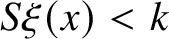 $S\xi (x)< k$
, we note that
$S\xi (x)< k$
, we note that
![]() . On the other hand, when comparing
. On the other hand, when comparing
 $\mathcal D(\xi, x)$
and
$\mathcal D(\xi, x)$
and
 $\mathcal D(\xi, x-1)$
, we see that if
$\mathcal D(\xi, x-1)$
, we see that if
 $i\leqslant k$
, then
$i\leqslant k$
, then
 $\mathcal D(\xi, x)$
loses one element, namely,
$\mathcal D(\xi, x)$
loses one element, namely,
 $z=\mathcal {H}_{i}(\gamma )$
, because
$z=\mathcal {H}_{i}(\gamma )$
, because
 $x=\mathcal {T}_{i}(\gamma ^{1})$
; but if
$x=\mathcal {T}_{i}(\gamma ^{1})$
; but if
 $A_{x}$
occurs, then
$A_{x}$
occurs, then
 $x=\mathcal {H}_{j}(\tilde \gamma )$
for some other soliton
$x=\mathcal {H}_{j}(\tilde \gamma )$
for some other soliton
 $\tilde \gamma $
and
$\tilde \gamma $
and
 $j\leqslant k$
, so that
$j\leqslant k$
, so that
 $x\in \mathcal D_{k}(\xi, x)$
. Putting all the pieces together, we conclude that (3.3) also holds in this case, which completes its proof.
$x\in \mathcal D_{k}(\xi, x)$
. Putting all the pieces together, we conclude that (3.3) also holds in this case, which completes its proof.
To see why (3.3) leads to the first statement in the theorem, let
 $\gamma $
be a k-soliton to the right of
$\gamma $
be a k-soliton to the right of
 $r(\xi, 0)=0$
. Let us check
$r(\xi, 0)=0$
. Let us check
 $D_{k}(\xi, x(\gamma ^{1}))=k$
.
$D_{k}(\xi, x(\gamma ^{1}))=k$
.
Firstly, suppose that
 $x(\gamma ^{1})=x(\gamma )=a$
. By Lemma 1.6, this can only happen if
$x(\gamma ^{1})=x(\gamma )=a$
. By Lemma 1.6, this can only happen if
 $I(\gamma )\subseteq I(\gamma ')$
for some
$I(\gamma )\subseteq I(\gamma ')$
for some
 $\gamma '$
. Let
$\gamma '$
. Let
 $\tilde \gamma $
be the largest soliton among such
$\tilde \gamma $
be the largest soliton among such
 $\gamma '$
, which exists by virtue of Lemma 1.5. Because
$\gamma '$
, which exists by virtue of Lemma 1.5. Because
 $\gamma $
has to be appended to a k-slot, and because it can be checked that there is no k-slot in
$\gamma $
has to be appended to a k-slot, and because it can be checked that there is no k-slot in
 $[x(\tilde \gamma ), \mathcal {H}_{k}(\tilde \gamma )]$
, we deduce that
$[x(\tilde \gamma ), \mathcal {H}_{k}(\tilde \gamma )]$
, we deduce that
 $\mathcal {H}_{1}(\tilde \gamma )< \dots <\mathcal {H}_{k}(\tilde \gamma )<a$
. Noting that
$\mathcal {H}_{1}(\tilde \gamma )< \dots <\mathcal {H}_{k}(\tilde \gamma )<a$
. Noting that
 $\mathcal {T}(\tilde \gamma ^{1})$
is on the right of
$\mathcal {T}(\tilde \gamma ^{1})$
is on the right of
 $\max I(\tilde \gamma )-1$
, we see that
$\max I(\tilde \gamma )-1$
, we see that
 $\mathcal {H}_{1}(\tilde \gamma ), \dots, \mathcal {H}_{k}(\tilde \gamma )\in \mathcal D_{k}(\xi, a)$
. On the other hand,
$\mathcal {H}_{1}(\tilde \gamma ), \dots, \mathcal {H}_{k}(\tilde \gamma )\in \mathcal D_{k}(\xi, a)$
. On the other hand,
 $\tilde \gamma $
is the only soliton in
$\tilde \gamma $
is the only soliton in
 $ \xi $
containing
$ \xi $
containing
 $\gamma $
that is appended to a record and therefore is also the only one that moves forward. If
$\gamma $
that is appended to a record and therefore is also the only one that moves forward. If
 $\widehat \gamma $
is another soliton satisfying
$\widehat \gamma $
is another soliton satisfying
 $x(\widehat \gamma )=\min I(\widehat \gamma )<a<\max I(\widehat \gamma ^{1})$
, then we must have
$x(\widehat \gamma )=\min I(\widehat \gamma )<a<\max I(\widehat \gamma ^{1})$
, then we must have
 $I(\widehat \gamma )\cap I(\gamma )=\varnothing $
. In particular,
$I(\widehat \gamma )\cap I(\gamma )=\varnothing $
. In particular,
 $\gamma $
is nested in the tail of
$\gamma $
is nested in the tail of
 $\widehat \gamma ^{1}$
; that is,
$\widehat \gamma ^{1}$
; that is,
 $a>\mathcal {T}_{1}(\widehat \gamma ^{1})$
. Moreover, the first k-slot after
$a>\mathcal {T}_{1}(\widehat \gamma ^{1})$
. Moreover, the first k-slot after
 $\mathcal {T}_{1}(\widehat \gamma ^{1})$
is
$\mathcal {T}_{1}(\widehat \gamma ^{1})$
is
 $\mathcal {T}_{k+1}(\widehat \gamma ^{1})$
. This implies
$\mathcal {T}_{k+1}(\widehat \gamma ^{1})$
. This implies
 $a\geqslant \mathcal {T}_{k+1}(\widehat \gamma ^{1})$
. We then conclude with
$a\geqslant \mathcal {T}_{k+1}(\widehat \gamma ^{1})$
. We then conclude with
 $D_{k}(\xi, a)=\#\mathcal D_{k}(\xi, a)=k$
.
$D_{k}(\xi, a)=\#\mathcal D_{k}(\xi, a)=k$
.
Secondly, suppose that
 $a'=x(\gamma ^{1})>x(\gamma )$
. Let us show
$a'=x(\gamma ^{1})>x(\gamma )$
. Let us show
 $\mathcal D_{k}(\xi, a')=\{\mathcal {H}_{1}(\gamma ), \dots, \mathcal {H}_{k}(\gamma )\}$
in this case. Indeed, if
$\mathcal D_{k}(\xi, a')=\{\mathcal {H}_{1}(\gamma ), \dots, \mathcal {H}_{k}(\gamma )\}$
in this case. Indeed, if
 $\widehat \gamma \ne \gamma $
is a soliton with
$\widehat \gamma \ne \gamma $
is a soliton with
 $x(\widehat \gamma )<a'<\max I(\widehat \gamma ^{1})$
, because
$x(\widehat \gamma )<a'<\max I(\widehat \gamma ^{1})$
, because
 $\gamma $
is appended to a record, we must have
$\gamma $
is appended to a record, we must have
 $I(\widehat \gamma )\cap I(\gamma )=\varnothing $
and
$I(\widehat \gamma )\cap I(\gamma )=\varnothing $
and
 $\widehat \gamma $
has size
$\widehat \gamma $
has size
 $>k$
. As previously, we deduce that
$>k$
. As previously, we deduce that
 $\gamma ^{1}$
is appended to a k-slot inside the tail of
$\gamma ^{1}$
is appended to a k-slot inside the tail of
 $\widehat \gamma ^{1}$
, so that
$\widehat \gamma ^{1}$
, so that
 $a'\geqslant \mathcal {T}_{k+1}(\widehat \gamma ^{1})$
. It follows that
$a'\geqslant \mathcal {T}_{k+1}(\widehat \gamma ^{1})$
. It follows that
 $\mathcal {H}_{i}(\widehat \gamma )\notin \mathcal D_{k}(\xi, a')$
for each
$\mathcal {H}_{i}(\widehat \gamma )\notin \mathcal D_{k}(\xi, a')$
for each
 $i\leqslant k$
, and therefore
$i\leqslant k$
, and therefore
 $D_{k}(\xi, a')=k$
.
$D_{k}(\xi, a')=k$
.
Now if
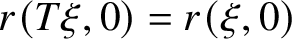 $r(T\xi, 0)=r(\xi, 0)$
, then Proposition 1.3 and Lemma 1.5 imply that
$r(T\xi, 0)=r(\xi, 0)$
, then Proposition 1.3 and Lemma 1.5 imply that
 $o^{1}_{k}(\xi )=0$
for all k. In the case that
$o^{1}_{k}(\xi )=0$
for all k. In the case that
 $x(\gamma ^{1})=x(\gamma )$
, the first statement in the theorem readily follows. If, on the other hand,
$x(\gamma ^{1})=x(\gamma )$
, the first statement in the theorem readily follows. If, on the other hand,
 $x(\gamma ^{1})>x(\gamma )$
, denote by
$x(\gamma ^{1})>x(\gamma )$
, denote by
 $\mathcal T_{1}$
the first site in the tail of
$\mathcal T_{1}$
the first site in the tail of
 $\gamma $
; then according to Proposition 1.3 and Lemma 1.6, we must have
$\gamma $
; then according to Proposition 1.3 and Lemma 1.6, we must have
 $x(\gamma ^{1})=\mathcal T_{1}$
. However,
$x(\gamma ^{1})=\mathcal T_{1}$
. However,
 $[x(\gamma ), \mathcal T_{1}]$
can only contain solitons of size
$[x(\gamma ), \mathcal T_{1}]$
can only contain solitons of size
 $\leqslant k$
by Lemma 1.5, from which it follows that
$\leqslant k$
by Lemma 1.5, from which it follows that
 $S_{k}\xi \cap [x(\gamma ), x(\gamma ^{1}))=\varnothing $
. So the first statement in the theorem also holds in this case. If
$S_{k}\xi \cap [x(\gamma ), x(\gamma ^{1}))=\varnothing $
. So the first statement in the theorem also holds in this case. If
 $r(T\xi, 0)<r(\xi, 0)$
, then we need to incorporate a further shift into the indices of k-slots, which is precisely given by
$r(T\xi, 0)<r(\xi, 0)$
, then we need to incorporate a further shift into the indices of k-slots, which is precisely given by
 $o^{1}_{k}(\xi )$
. If
$o^{1}_{k}(\xi )$
. If
 $\gamma $
is to the left of
$\gamma $
is to the left of
 $r(\xi, 0)$
, the arguments are similar: it suffices to note that after each iteration, the soliton loses
$r(\xi, 0)$
, the arguments are similar: it suffices to note that after each iteration, the soliton loses
 $k \ k$
-slots on the right.
$k \ k$
-slots on the right.
To extend to an infinite configuration
 $\xi \in \mathcal {W}$
, let us take
$\xi \in \mathcal {W}$
, let us take
 $x\in \mathbb {Z}$
and let
$x\in \mathbb {Z}$
and let
 $r(x)$
be the rightmost record of
$r(x)$
be the rightmost record of
 $\xi $
preceding x. We note that
$\xi $
preceding x. We note that
 $T\xi |_{[r(x), x]}$
only depends on
$T\xi |_{[r(x), x]}$
only depends on
 $\xi |_{[r(x), x]}$
in the sense that if
$\xi |_{[r(x), x]}$
in the sense that if
 $\xi '$
is a finite configuration with
$\xi '$
is a finite configuration with
 $\xi '(y)=\xi (y)$
for all
$\xi '(y)=\xi (y)$
for all
 $y\in [r(x), x]$
and
$y\in [r(x), x]$
and
 $r(x)$
being a record of
$r(x)$
being a record of
 $\xi '$
, then
$\xi '$
, then
 $T\xi (y)=T\xi '(y)$
for all
$T\xi (y)=T\xi '(y)$
for all
 $y\in [r(x), x]$
. Because solitons are contained in excursions, we also have
$y\in [r(x), x]$
. Because solitons are contained in excursions, we also have
 $S\xi (y)=S\xi '(y)$
for
$S\xi (y)=S\xi '(y)$
for
 $y\in [r(x), x]$
. Let
$y\in [r(x), x]$
. Let
 $r'(x)=r(T\xi, -\xi (r(x)))\leqslant r(x)$
be the record in
$r'(x)=r(T\xi, -\xi (r(x)))\leqslant r(x)$
be the record in
 $T\xi $
that replaces
$T\xi $
that replaces
 $r(x)$
. Then the same argument implies that
$r(x)$
. Then the same argument implies that
 $ST\xi (x)$
only depends on
$ST\xi (x)$
only depends on
 $T\xi |_{[r'(x), x]}$
, which in its turn only depends on
$T\xi |_{[r'(x), x]}$
, which in its turn only depends on
 $\xi |_{[r(r'(x)), x]}$
. Therefore, if we take a large enough box
$\xi |_{[r(r'(x)), x]}$
. Therefore, if we take a large enough box
 $[-n, n]$
containing
$[-n, n]$
containing
 $[r(r'(x)), x]$
as well as
$[r(r'(x)), x]$
as well as
 $r(r(T\xi, 0))$
, then the restriction of
$r(r(T\xi, 0))$
, then the restriction of
 $\xi $
to this box is enough to determine the truncated k-slot configurations
$\xi $
to this box is enough to determine the truncated k-slot configurations
 $(s_{k}(\xi, i))_{i\leqslant i_{0}}$
with
$(s_{k}(\xi, i))_{i\leqslant i_{0}}$
with
 $i_{0}=\max \{i: s_{k}(\xi, i)\leqslant x\}$
and
$i_{0}=\max \{i: s_{k}(\xi, i)\leqslant x\}$
and
 $(s_{k}(T\xi, i))_{i\leqslant i^{\prime }_{0}}$
with
$(s_{k}(T\xi, i))_{i\leqslant i^{\prime }_{0}}$
with
 $i^{\prime }_{0}=\max \{i: s_{k}(T\xi, i)\leqslant x\}$
. Hence, the first statement of the theorem also holds for a general
$i^{\prime }_{0}=\max \{i: s_{k}(T\xi, i)\leqslant x\}$
. Hence, the first statement of the theorem also holds for a general
 $\xi \in \mathcal {W}$
.
$\xi \in \mathcal {W}$
.
For the third statement, suppose that
 $\xi,\xi '\in \mathcal {W}$
satisfy
$\xi,\xi '\in \mathcal {W}$
satisfy
 $(M_m\xi :m>k)=(M_m\xi ':m>k)$
; let us show that
$(M_m\xi :m>k)=(M_m\xi ':m>k)$
; let us show that
 $J^{1}_{m}\xi =J^{1}_{m}\xi '$
for all
$J^{1}_{m}\xi =J^{1}_{m}\xi '$
for all
 $m> k$
, from which it will follow that
$m> k$
, from which it will follow that
 $o^t_k(\xi )= o^t_k(\xi ')$
by (3.1). We have seen that there exists some
$o^t_k(\xi )= o^t_k(\xi ')$
by (3.1). We have seen that there exists some
 $k_{0}(\xi )\in \mathbb {N}$
(respectively
$k_{0}(\xi )\in \mathbb {N}$
(respectively
 $k_{0}(\xi ')\in \mathbb {N}$
) such that
$k_{0}(\xi ')\in \mathbb {N}$
) such that
 $J^{1}_{m}\xi =0$
for all
$J^{1}_{m}\xi =0$
for all
 $m\geqslant k_{0}(\xi )$
(respectively
$m\geqslant k_{0}(\xi )$
(respectively
 $J^{1}_{m}\xi '=0$
for all
$J^{1}_{m}\xi '=0$
for all
 $m\geqslant k_{0}(\xi ')$
). Taking
$m\geqslant k_{0}(\xi ')$
). Taking
 $k_{0}=\max (k_{0}(\xi ), k_{0}(\xi '))$
, we see that
$k_{0}=\max (k_{0}(\xi ), k_{0}(\xi '))$
, we see that
 $J^{1}_{m}\xi =J^{1}_{m}\xi '=0$
for all
$J^{1}_{m}\xi =J^{1}_{m}\xi '=0$
for all
 $m\geqslant k_{0}$
. For
$m\geqslant k_{0}$
. For
 $k=k_0-1$
, we immediately deduce
$k=k_0-1$
, we immediately deduce
 $o^1_k(\xi )=o^{1}_{k}(\xi ')=0$
by (3.1). Moreover, we have
$o^1_k(\xi )=o^{1}_{k}(\xi ')=0$
by (3.1). Moreover, we have
 $J^{1}_{k}\xi $
counting the number of k-solitons crossing record
$J^{1}_{k}\xi $
counting the number of k-solitons crossing record
 $0$
, namely, the k-solitons appended to a k-slot with a negative index at time
$0$
, namely, the k-solitons appended to a k-slot with a negative index at time
 $0$
and then appended to a positive-indexed k-slot at time
$0$
and then appended to a positive-indexed k-slot at time
 $1$
. Thus,
$1$
. Thus,
 $J^{1}_{k}\xi = \sum _{i=0}^{k-1}M_{k}T\xi (i)=\sum _{i=-k}^{-1}M_{k}\xi (i)$
, by the second statement of the theorem. A similar identity holds for
$J^{1}_{k}\xi = \sum _{i=0}^{k-1}M_{k}T\xi (i)=\sum _{i=-k}^{-1}M_{k}\xi (i)$
, by the second statement of the theorem. A similar identity holds for
 $J^{1}_{k}\xi '$
. Therefore, if
$J^{1}_{k}\xi '$
. Therefore, if
 $k=k_{0}-2$
, we have
$k=k_{0}-2$
, we have
 $J^{1}_{m}\xi =J^{1}_{m}\xi '$
for all
$J^{1}_{m}\xi =J^{1}_{m}\xi '$
for all
 $m>k$
and so
$m>k$
and so
 $o^t_k(\xi )= o^t_k(\xi ')$
. Proceeding by downward induction, the same will be true for
$o^t_k(\xi )= o^t_k(\xi ')$
. Proceeding by downward induction, the same will be true for
 $k=k_0-2,k_0-3,\dots,2,1$
. This concludes the proof of Theorem 3.1.
$k=k_0-2,k_0-3,\dots,2,1$
. This concludes the proof of Theorem 3.1.
4 Invariant measures
It is known that stationary Markov chains on
 $ \{0,1\} $
with density of 1s less than
$ \{0,1\} $
with density of 1s less than
 $\frac 12$
are T-invariant,Footnote
1
but in fact there are many other invariant measures for the BBS. This is due to the existence of many conservation laws intrinsic to this dynamics, in particular, the conservation of solitons studied in the previous section
$\frac 12$
are T-invariant,Footnote
1
but in fact there are many other invariant measures for the BBS. This is due to the existence of many conservation laws intrinsic to this dynamics, in particular, the conservation of solitons studied in the previous section
In this section we prove Theorem 1.5. More precisely, we show explicitly how invariant measures can be constructed by specifying the distribution of each kth component
 $\zeta _k$
.
$\zeta _k$
.
We will refer to probability measures as simply measures. We will also refer to measurable functions as random elements and refer to the pushforward of a prespecified measure by such functions as the law of these random elements. A measure
 $\mu $
on
$\mu $
on
 $\mathcal {X}$
is T-invariant if
$\mathcal {X}$
is T-invariant if
 $\mu \circ T^{-1} = \mu $
.
$\mu \circ T^{-1} = \mu $
.
4.1 Construction of the measures
Our recipe to produce invariant measures uses the construction described in Subsection 2.2, and it gives a distribution
 $\widehat {\mu }$
of configurations ‘seen from a typical record’. The proof of Theorem 1.5 is based on properties of
$\widehat {\mu }$
of configurations ‘seen from a typical record’. The proof of Theorem 1.5 is based on properties of
 $\widehat {\mu }$
and how they relate to the dynamics. This relationship is given by the Palm theory, which we briefly recall now.
$\widehat {\mu }$
and how they relate to the dynamics. This relationship is given by the Palm theory, which we briefly recall now.
Let
 $\eta \in \{0,1\}^{\mathbb {Z}}$
. From (1.1) and (1.8), we have
$\eta \in \{0,1\}^{\mathbb {Z}}$
. From (1.1) and (1.8), we have
 $\theta R \eta = R \theta \eta $
. Suppose that
$\theta R \eta = R \theta \eta $
. Suppose that
 $\eta \in \mathcal {X}$
, and denote
$\eta \in \mathcal {X}$
, and denote
 $$ \begin{align*} \mathtt r(\eta) := \inf\{x\geqslant 1: x \in R\eta\}. \end{align*} $$
If
 $ \eta $
is random with law
$ \eta $
is random with law
 $ \widehat {\mu } $
such that
$ \widehat {\mu } $
such that
 $\widehat {\mu }(\mathtt r):=\int \mathtt r(\eta )\,\widehat {\mu }(\mathrm {d}\eta ) <\infty $
, its inverse-Palm measure
$\widehat {\mu }(\mathtt r):=\int \mathtt r(\eta )\,\widehat {\mu }(\mathrm {d}\eta ) <\infty $
, its inverse-Palm measure
 $\mu =\operatorname {\mathrm {Palm}}_{R}^{\mathbb {Z}}(\widehat {\mu })$
is defined as follows. For every test function
$\mu =\operatorname {\mathrm {Palm}}_{R}^{\mathbb {Z}}(\widehat {\mu })$
is defined as follows. For every test function
 $\varphi $
,
$\varphi $
,
 $$ \begin{align} \int \varphi(\eta) \,\mu(\mathrm{d}\eta) := \int \frac{\textstyle\sum_{i=0}^{\mathtt r(\eta)-1} \varphi(\theta^i\eta)} {\mathtt r(\eta)} \cdot \frac{\mathtt r(\eta)}{\widehat{\mu}(\mathtt r)} \widehat{\mu}(\mathrm{d}\eta). \end{align} $$
Informally, to sample a configuration distributed as
 $\mu $
one can first sample a configuration using the distribution
$\mu $
one can first sample a configuration using the distribution
 $\widehat {\mu }$
biased by the length of the first excursion (when
$\widehat {\mu }$
biased by the length of the first excursion (when
 $ 0\in R\eta $
) and then choose a site uniformly from this excursion (along with the record preceding it) to place the origin.
$ 0\in R\eta $
) and then choose a site uniformly from this excursion (along with the record preceding it) to place the origin.
For
 $ \eta \in \mathcal {X} $
, we define the record-shift operator
$ \eta \in \mathcal {X} $
, we define the record-shift operator
 $\widehat {\theta }$
as
$\widehat {\theta }$
as
 $$ \begin{align*} \widehat{\theta} \eta := \theta^{\mathtt r(\eta)}\eta. \end{align*} $$
We also define the dynamics seen from a record
 $\widehat {T}:\skew8\widehat{\mathcal {X}}\to \skew8\widehat{\mathcal {X}}$
by
$\widehat {T}:\skew8\widehat{\mathcal {X}}\to \skew8\widehat{\mathcal {X}}$
by
 $$ \begin{align} \widehat{T} \eta := \theta^{r(T \xi^{\circ}[\eta],0)}T\eta, \end{align} $$
where
 $\xi ^{\circ }[\eta ]$
was defined in Subsection 2.2 as the unique lift of
$\xi ^{\circ }[\eta ]$
was defined in Subsection 2.2 as the unique lift of
 $\eta $
with record
$\eta $
with record
 $0$
at
$0$
at
 $0$
. In words,
$0$
. In words,
 $ \widehat {T} $
means apply
$ \widehat {T} $
means apply
 $ T $
and recenter the configuration at the new position of record 0. The following lemma follows from standard properties of Palm measures and is proved in Section 5.
$ T $
and recenter the configuration at the new position of record 0. The following lemma follows from standard properties of Palm measures and is proved in Section 5.
Lemma 4.3. Let
 $\widehat {\mu }$
be a probability measure of
$\widehat {\mu }$
be a probability measure of
 $\{0, 1\}^{\mathbb {Z}}$
. Suppose that
$\{0, 1\}^{\mathbb {Z}}$
. Suppose that
 $\widehat {\mu }(0\in R\eta )=1$
,
$\widehat {\mu }(0\in R\eta )=1$
,
 $\widehat {\mu }(\mathtt r)< \infty $
,
$\widehat {\mu }(\mathtt r)< \infty $
,
 $\widehat {\mu }$
is
$\widehat {\mu }$
is
 $\widehat {\theta }$
-invariant and
$\widehat {\theta }$
-invariant and
 $\widehat {\mu }(R\eta =\mathbb {Z})=0$
. Then
$\widehat {\mu }(R\eta =\mathbb {Z})=0$
. Then
 $\widehat {\mu }$
is supported on
$\widehat {\mu }$
is supported on
 $\skew8\widehat{\mathcal {X}}$
, and
$\skew8\widehat{\mathcal {X}}$
, and
 $\operatorname {\mathrm {Palm}}_{R}^{\mathbb {Z}}(\widehat {\mu })$
is
$\operatorname {\mathrm {Palm}}_{R}^{\mathbb {Z}}(\widehat {\mu })$
is
 $\theta $
-invariant, supported on
$\theta $
-invariant, supported on
 $\mathcal {X}$
and satisfies
$\mathcal {X}$
and satisfies
 $$ \begin{align*} \operatorname{\mathrm{Palm}}_{R}^{\mathbb{Z}}(\widehat{\mu}) \circ T^{-1} = \operatorname{\mathrm{Palm}}_{R}^{\mathbb{Z}}(\widehat{\mu} \circ \widehat{T}^{-1}). \end{align*} $$
If, moreover,
 $\widehat {\mu }$
is
$\widehat {\mu }$
is
 $\widehat {\theta }$
-ergodic, then
$\widehat {\theta }$
-ergodic, then
 $\operatorname {\mathrm {Palm}}_{R}^{\mathbb {Z}}(\widehat {\mu })$
is
$\operatorname {\mathrm {Palm}}_{R}^{\mathbb {Z}}(\widehat {\mu })$
is
 $\theta $
-ergodic.
$\theta $
-ergodic.
We now introduce the assumptions and notation used throughout the rest of this section.
Let
 $\zeta =(\zeta _k)_{k\geqslant 1}$
be a sequence of independent random elements of
$\zeta =(\zeta _k)_{k\geqslant 1}$
be a sequence of independent random elements of
 $(\mathbb {Z}_{+})^{\mathbb {Z}}$
with shift-invariant distributions. Let
$(\mathbb {Z}_{+})^{\mathbb {Z}}$
with shift-invariant distributions. Let
 $ P $
and
$ P $
and
 $ E $
denote the underlying probability measure and expectation and suppose that the law of
$ E $
denote the underlying probability measure and expectation and suppose that the law of
 $ \zeta $
satisfies
$ \zeta $
satisfies
 $\sum _k k E[\zeta _k(0)] <\infty $
and
$\sum _k k E[\zeta _k(0)] <\infty $
and
 $P(\sum _{k,i}\zeta _{k}(i)>0)=1$
. In particular, this implies that the random field
$P(\sum _{k,i}\zeta _{k}(i)>0)=1$
. In particular, this implies that the random field
 $\zeta $
a.s. satisfies (2.3) by Borel–Cantelli. Take
$\zeta $
a.s. satisfies (2.3) by Borel–Cantelli. Take
 $\xi =M^{-1} \zeta $
as the walk reconstructed from
$\xi =M^{-1} \zeta $
as the walk reconstructed from
 $\zeta $
according to the algorithm described in Subsection 2.2 and depicted in Figure 2.6. Let
$\zeta $
according to the algorithm described in Subsection 2.2 and depicted in Figure 2.6. Let
 $\widehat {\mu }$
denote the resulting law of
$\widehat {\mu }$
denote the resulting law of
 $\eta =\eta [\xi ]$
.
$\eta =\eta [\xi ]$
.
Proposition 4.4. The measure
 $\widehat {\mu }$
defined above is
$\widehat {\mu }$
defined above is
 $\widehat {T}$
-invariant and
$\widehat {T}$
-invariant and
 $\widehat {\theta }$
-invariant, and it also satisfies
$\widehat {\theta }$
-invariant, and it also satisfies
 $\widehat {\mu }(\mathtt r)<\infty $
and
$\widehat {\mu }(\mathtt r)<\infty $
and
 $\widehat {\mu }(R\eta =\mathbb {Z})=0$
. If, moreover,
$\widehat {\mu }(R\eta =\mathbb {Z})=0$
. If, moreover,
 $(\zeta _k(i))_{i\in \mathbb {Z}}$
is i.i.d. for each k, then
$(\zeta _k(i))_{i\in \mathbb {Z}}$
is i.i.d. for each k, then
 $\widehat {\mu }$
is also
$\widehat {\mu }$
is also
 $\widehat {\theta }$
-ergodic.
$\widehat {\theta }$
-ergodic.
Before giving the proof, let us see how it implies Theorem 1.5.
Proof of Theorem 1.5. Let
 $\widehat {\mu }$
be the law of
$\widehat {\mu }$
be the law of
 $\eta = M^{-1}\zeta $
, and define
$\eta = M^{-1}\zeta $
, and define
 $$ \begin{align*} \mu:=\operatorname{\mathrm{Palm}}_{R}^{\mathbb{Z}}(\widehat{\mu}). \end{align*} $$
By Proposition 4.4 and Lemma 4.3,
 $\mu $
is
$\mu $
is
 $\theta $
-invariant and supported on
$\theta $
-invariant and supported on
 $\mathcal {X}$
. Also,
$\mathcal {X}$
. Also,
 $$ \begin{align*}\mu\circ T^{-1} = \operatorname{\mathrm{Palm}}_{R}^{\mathbb{Z}}(\widehat{\mu}\circ\widehat{T}^{-1})=\operatorname{\mathrm{Palm}}_{R}^{\mathbb{Z}}(\widehat{\mu})=\mu,\end{align*} $$
so
 $\mu $
is also T-invariant. Moreover, under the i.i.d. assumption, the second part of Proposition 4.4 combined with the second part of Lemma 4.3 implies that
$\mu $
is also T-invariant. Moreover, under the i.i.d. assumption, the second part of Proposition 4.4 combined with the second part of Lemma 4.3 implies that
 $\mu $
is
$\mu $
is
 $\theta $
-ergodic.
$\theta $
-ergodic.
Remark 4.5 i.i.d. measures
A natural question is whether the product measures
 $\nu _\lambda $
can be constructed in this way. This is indeed the case, as shown in [Reference Ferrari and GabrielliFG20a].
$\nu _\lambda $
can be constructed in this way. This is indeed the case, as shown in [Reference Ferrari and GabrielliFG20a].
Example 4.6 Ergodicity without independent components
It is possible for law
 $\mu $
of
$\mu $
of
 $\eta $
to be
$\eta $
to be
 $\theta $
-ergodic and T-invariant while its components
$\theta $
-ergodic and T-invariant while its components
 $M_k \eta $
are not independent under
$M_k \eta $
are not independent under
 $\widehat {\mu }$
. Let
$\widehat {\mu }$
. Let
 $\zeta '$
be the configuration
$\zeta '$
be the configuration
![]() . Let
. Let
 $\zeta _1=\zeta _4$
be a configuration chosen uniformly at random in the set
$\zeta _1=\zeta _4$
be a configuration chosen uniformly at random in the set
 $\{\zeta ', \theta \zeta ', \theta ^2\zeta '\}$
; let
$\{\zeta ', \theta \zeta ', \theta ^2\zeta '\}$
; let
 $\zeta _k\equiv 0$
for all
$\zeta _k\equiv 0$
for all
 $k\notin \{1,4\}$
and
$k\notin \{1,4\}$
and
 $\zeta =(\zeta _k)_{k\geqslant 1}$
. The reader can check that this example satisfies the stated properties. The resulting configuration is periodic for
$\zeta =(\zeta _k)_{k\geqslant 1}$
. The reader can check that this example satisfies the stated properties. The resulting configuration is periodic for
 $ \theta $
and invariant for
$ \theta $
and invariant for
 $ T $
:
$ T $
:
 $$ \begin{align*} \cdots 00{\color{blue} 10}{\color{red} 1111}{{\color{blue} 01}}{\color{red} 0000}{{\color{blue} 10}}000{{\color{blue} 10}}{\color{red} 1111}{{\color{blue} 01}}{\color{red} 0000}{{\color{blue} 10}}0 \cdots, \end{align*} $$
where colors (online) represent records,
 $ 4 $
-solitons and
$ 4 $
-solitons and
 $ 1 $
-solitons.
$ 1 $
-solitons.
Example 4.7 Independent components without ergodicity
It is also possible for
 $\zeta $
to be independent over k,
$\zeta $
to be independent over k,
 $\theta $
-ergodic for each k but produce (by the above procedure) a configuration
$\theta $
-ergodic for each k but produce (by the above procedure) a configuration
 $\eta $
whose law is not
$\eta $
whose law is not
 $\theta $
-ergodic. To see that, take
$\theta $
-ergodic. To see that, take
 $\zeta _5(x)\equiv 1$
,
$\zeta _5(x)\equiv 1$
,
 $\zeta _1$
as in the previous example,
$\zeta _1$
as in the previous example,
 $\zeta _k\equiv 0$
for all
$\zeta _k\equiv 0$
for all
 $k\notin \{1,5\}$
and
$k\notin \{1,5\}$
and
 $\zeta =(\zeta _k)_{k\geqslant 1}$
. The resulting configurations give three classes periodic for
$\zeta =(\zeta _k)_{k\geqslant 1}$
. The resulting configurations give three classes periodic for
 $ \theta $
and cyclic over
$ \theta $
and cyclic over
 $ T $
:
$ T $
:
 $$ \begin{align*} \cdots 0{{\color{blue} 10}}{\color{red} 1111}{{\color{blue} 01}}{\color{red} 1000}{{\color{blue} 10}}{\color{red} 00} 0{{\color{blue} 10}}{\color{red} 1111}{{\color{blue} 01}}{\color{red} 1000}{{\color{blue} 10}}{\color{red} 00} \cdots \\ \cdots 0{\color{red} 111}{{\color{blue} 01}}{\color{red} 1100}{{\color{blue} 10}}{\color{red} 000}{{\color{blue} 10}} 0{\color{red} 111}{{\color{blue} 01}}{\color{red} 1100}{{\color{blue} 10}}{\color{red} 000}{{\color{blue} 10}} \cdots \\ \cdots 0{\color{red} 11}{{\color{blue} 01}}{\color{red} 111}{{\color{blue} 01}}{\color{red} 0000}{{\color{blue} 10}}{\color{red} 0} 0{\color{red} 11}{{\color{blue} 01}}{\color{red} 111}{{\color{blue} 01}}{\color{red} 0000}{{\color{blue} 10}}{\color{red} 0} \cdots \end{align*} $$
where colors (online) represent records,
 $ 5 $
-solitons and
$ 5 $
-solitons and
 $ 1 $
-solitons.
$ 1 $
-solitons.
Remark 4.8. A measure
 $\mu $
is said to be
$\mu $
is said to be
 $\theta $
-mixing if for all
$\theta $
-mixing if for all
 $A, B \in \mathcal {B}$
,
$A, B \in \mathcal {B}$
,
 $\mu (A\cap \theta ^{-n}B) {\to } \mu (A)\mu (B)$
as
$\mu (A\cap \theta ^{-n}B) {\to } \mu (A)\mu (B)$
as
 $ n\to \infty $
. We conjecture that, for every measure
$ n\to \infty $
. We conjecture that, for every measure
 $ \mu $
supported on
$ \mu $
supported on
 $ \mathcal {X} $
,
$ \mathcal {X} $
,
 $ \mu $
is T-invariant and
$ \mu $
is T-invariant and
 $\theta $
-mixing if and only if under
$\theta $
-mixing if and only if under
 $ \widehat {\mu } $
the components
$ \widehat {\mu } $
the components
 $\zeta _k$
are independent over k and each one is
$\zeta _k$
are independent over k and each one is
 $\theta $
-mixing.
$\theta $
-mixing.
4.2 Invariance of the reconstructed configuration
We now prove the main part of Proposition 4.4, namely,
 $\widehat {\theta }$
-invariance and
$\widehat {\theta }$
-invariance and
 $\widehat {T}$
-invariance of
$\widehat {T}$
-invariance of
 $\widehat {\mu }$
, as well as
$\widehat {\mu }$
, as well as
 $\theta $
-ergodicity in case of i.i.d. components. The proof of
$\theta $
-ergodicity in case of i.i.d. components. The proof of
 $\widehat {\mu }(\mathtt r)<\infty $
is given in Subsection 4.3. The condition
$\widehat {\mu }(\mathtt r)<\infty $
is given in Subsection 4.3. The condition
 $\widehat {\mu }(R\eta =\mathbb {Z})=0$
is easily checked from the construction of
$\widehat {\mu }(R\eta =\mathbb {Z})=0$
is easily checked from the construction of
 $M^{-1}\zeta $
and the assumption
$M^{-1}\zeta $
and the assumption
 $\sum _{k,i}\zeta _{k}(i)>0$
a.s. Denote by
$\sum _{k,i}\zeta _{k}(i)>0$
a.s. Denote by
 $\mathcal {F}_k$
the sigma-field generated by
$\mathcal {F}_k$
the sigma-field generated by
 $(\zeta _m)_{m>k}$
.
$(\zeta _m)_{m>k}$
.
Because one can write
 $\eta = M^{-1}M\eta $
and
$\eta = M^{-1}M\eta $
and
 $\widehat {T} \eta = M^{-1}M\widehat {T}\eta $
by Theorem 1.3, it suffices to show that the slot decompositions
$\widehat {T} \eta = M^{-1}M\widehat {T}\eta $
by Theorem 1.3, it suffices to show that the slot decompositions
 $M\eta $
and
$M\eta $
and
 $M\widehat {T}\eta $
have the same law. More precisely, it suffices to show
$M\widehat {T}\eta $
have the same law. More precisely, it suffices to show
 $$ \begin{align} E\left(\prod_{k=1}^n \varphi_k(M_k\widehat{T}\eta)\right) = \prod_{k=1}^n E \varphi_k(\zeta_k) \end{align} $$
for test functions
 $\varphi _1,\dots,\varphi _n$
and
$\varphi _1,\dots,\varphi _n$
and
 $n \in \mathbb {N}$
.
$n \in \mathbb {N}$
.
We proceed by an induction on n. First, recall the notation from (4.2) and note that
 $$ \begin{align*} &E\big(\varphi_k(M_k\widehat{T}\eta)\,\big|\, \mathcal{F}_k \big)\\ &\qquad= E\big(\varphi_k(\theta^{-o^1_k(\xi^{\circ}[\eta])-k}M_k\eta)\,\big|\, \mathcal{F}_k \big) \qquad (\text{by Theorem~3.1}) \\ &\qquad= E\big(\varphi_k(\theta^{-o^1_k(\xi^{\circ}[\eta])-k}\zeta_k)\,\big|\, \mathcal{F}_k \big) \qquad (\text{because }M_k\eta=\zeta_k) \\ &\qquad= E\varphi_k(\zeta_k), \end{align*} $$
because
 $\zeta _k$
is shift-invariant and independent of
$\zeta _k$
is shift-invariant and independent of
 $(\zeta _m)_{m>k}$
, whereas
$(\zeta _m)_{m>k}$
, whereas
 $o^1_k(\xi ^{\circ }[\eta ])$
is determined by these elements. The inductive step to show (4.9) is then
$o^1_k(\xi ^{\circ }[\eta ])$
is determined by these elements. The inductive step to show (4.9) is then
 $$ \begin{align*} E\left(\prod_{i=k}^n \varphi_i(M_i\widehat{T}\eta)\right) &= E\left(E\left(\prod_{i=k}^n \varphi_i(M_i\widehat{T}\eta)\bigg| \mathcal{F}_k \right)\right),\\ \phantom{E\Bigl(\prod_{i=k}^n \varphi_i(M_i\widehat{T}\eta)\Bigr)} &= E\left( \prod_{i=k+1}^n \varphi_i(M_i\widehat{T}\eta) E\left(\varphi_k(M_k\widehat{T}\eta)\Big| \mathcal{F}_k \right)\right),\\ \phantom{E\left(\prod_{i=k}^n \varphi_i(M_i\widehat{T}\eta)\right)} &= E \varphi_k(\zeta_k) \ E\left(\prod_{i=k+1}^{n} \varphi_i(M_i\widehat{T}\eta)\right); \end{align*} $$
in the second identity we have used that
 $M_i\widehat {T}\eta $
is determined by
$M_i\widehat {T}\eta $
is determined by
 $(\zeta _m)_{m\geqslant i}$
by the last statement of Theorem 3.1. This shows that
$(\zeta _m)_{m\geqslant i}$
by the last statement of Theorem 3.1. This shows that
 $\widehat {\mu }$
is
$\widehat {\mu }$
is
 $\widehat {T}$
-invariant.
$\widehat {T}$
-invariant.
We now prove
 $ \widehat {\theta } $
-invariance. Consider the transformation
$ \widehat {\theta } $
-invariance. Consider the transformation
 $M^{-1} : \zeta \mapsto \xi ^*$
defined in Subsection 2.2 and denote
$M^{-1} : \zeta \mapsto \xi ^*$
defined in Subsection 2.2 and denote
 $\eta ^{*}=\eta [\xi ^{*}]$
the corresponding ball configuration. Call
$\eta ^{*}=\eta [\xi ^{*}]$
the corresponding ball configuration. Call
 $\varepsilon ^0_*$
the excursion of
$\varepsilon ^0_*$
the excursion of
 $\eta ^*$
between records 0 and 1. The construction of Subsection 2.2 gives
$\eta ^*$
between records 0 and 1. The construction of Subsection 2.2 gives
 $$ \begin{align*} \widehat{\theta} \eta^* = \theta^{r(\xi^{\circ}[\eta^*],1)}\eta^* = M^{-1} \big(\theta^{n_k(\varepsilon^0_*)}\zeta_k: k\geqslant 1\big). \end{align*} $$
So it suffices to show that
 $( \theta ^{n_k(\varepsilon ^0_*)}\zeta _k )_{k\geqslant 1}$
has the same law as
$( \theta ^{n_k(\varepsilon ^0_*)}\zeta _k )_{k\geqslant 1}$
has the same law as
 $(\zeta _k)_{k \geqslant 1}$
. But
$(\zeta _k)_{k \geqslant 1}$
. But
 $n_k(\varepsilon ^0_*)$
is determined by
$n_k(\varepsilon ^0_*)$
is determined by
 $(\zeta _m)_{m>k}$
and thus is independent of
$(\zeta _m)_{m>k}$
and thus is independent of
 $\zeta _k$
. Hence, the law of
$\zeta _k$
. Hence, the law of
 $\zeta _k$
is invariant by the random shift of
$\zeta _k$
is invariant by the random shift of
 $n_k(\varepsilon ^0_*)$
and it is independent of
$n_k(\varepsilon ^0_*)$
and it is independent of
 $(\zeta _m)_{m>k}$
. This shows that
$(\zeta _m)_{m>k}$
. This shows that
 $ \eta ^* $
and
$ \eta ^* $
and
 $ \widehat {\theta } \eta ^* $
have the same law.
$ \widehat {\theta } \eta ^* $
have the same law.
Finally, under the extra assumption that
 $(\zeta _k(i))_{i\in \mathbb {Z}}$
is i.i.d. for each k, the reconstruction map mentioned above will produce an i.i.d. sequence of excursions separated by records. This in turn implies that the resulting configuration
$(\zeta _k(i))_{i\in \mathbb {Z}}$
is i.i.d. for each k, the reconstruction map mentioned above will produce an i.i.d. sequence of excursions separated by records. This in turn implies that the resulting configuration
 $\eta $
is
$\eta $
is
 $\widehat {\theta }$
-ergodic.
$\widehat {\theta }$
-ergodic.
4.3 Expected excursion length
We continue with the proof of Proposition 4.4 to prove that
 $\widehat {\mu }(\mathtt r)<\infty $
. Let
$\widehat {\mu }(\mathtt r)<\infty $
. Let
 $$ \begin{align} \alpha_k := E[\zeta_k(0)]. \end{align} $$
The proof consists of two steps: first, we show that the following system
 $$ \begin{align} w_k = 1 + {\sum_{m>k}} 2(m-k) w_m\alpha_m,\qquad k=0,1,2,\dots \end{align} $$
has a unique finite nonnegative solution
 $w=(w_k)_{k\geqslant 0}$
; that is,
$w=(w_k)_{k\geqslant 0}$
; that is,
 $ w \in [0,\infty )^{\mathbb {N}_0} $
; second, we show that the average number of k-slots per excursion in
$ w \in [0,\infty )^{\mathbb {N}_0} $
; second, we show that the average number of k-slots per excursion in
 $M^{-1} \zeta $
is
$M^{-1} \zeta $
is
 $w_k$
, whence the average number of k-solitons per excursion satisfies
$w_k$
, whence the average number of k-solitons per excursion satisfies
 $$ \begin{align} \rho_k=\alpha_k w_k. \end{align} $$
In particular, this will imply that the average size of the excursions (along with the record preceding them) satisfies
 $$ \begin{align} \widehat{\mu}(\mathtt r) = w_0 = 1 + \sum_{m\geqslant1} 2m\, \rho_m <\infty. \end{align} $$
So we start by studying (4.11). Let c
k
:= 2
 $\sum$
m
$\sum$
m
 $>$
k
(m
$>$
k
(m
 $-$
k)
$-$
k)
 $\alpha$
m
. Because
$\alpha$
m
. Because
 $\sum _{k} k E[\zeta _{k}(0)]<\infty $
, we can take
$\sum _{k} k E[\zeta _{k}(0)]<\infty $
, we can take
 $\tilde {k}$
such that
$\tilde {k}$
such that
 $\sum$
m
$\sum$
m
 $>$
k~4m
$>$
k~4m
 $\alpha$
m
$\alpha$
m
 $<$
1, so
$<$
1, so
 $c_k< \frac {1}{2}$
for
$c_k< \frac {1}{2}$
for
 $k\geqslant \tilde k$
. Let
$k\geqslant \tilde k$
. Let
 $K:= \{k\in \mathbb {N}:k\geqslant \tilde k\}\cup \{\aleph \}$
and consider a Markov chain
$K:= \{k\in \mathbb {N}:k\geqslant \tilde k\}\cup \{\aleph \}$
and consider a Markov chain
 $(X_n)_{n\geqslant 0}$
on K with absorbing state
$(X_n)_{n\geqslant 0}$
on K with absorbing state
 $\aleph $
and transition probabilities
$\aleph $
and transition probabilities
;
 $q_{k,\aleph } = 1-c_k$
;
$q_{k,\aleph } = 1-c_k$
;
 $q_{\aleph,\aleph }=1$
and
$q_{\aleph,\aleph }=1$
and
 $q_{k,m}=0$
otherwise. Define the absorption time by
$q_{k,m}=0$
otherwise. Define the absorption time by
 $\tau := \inf \{n\geqslant 0: X_n=\aleph \}$
. Denote by
$\tau := \inf \{n\geqslant 0: X_n=\aleph \}$
. Denote by
 $P_k$
the law of
$P_k$
the law of
 $(X_n)_{n\geqslant 0}$
starting from k and by
$(X_n)_{n\geqslant 0}$
starting from k and by
 $ E_k $
the expectation. Applying the Markov property at time
$ E_k $
the expectation. Applying the Markov property at time
 $1$
, we see that
$1$
, we see that
 $w_k := E_k\tau $
satisfies
$w_k := E_k\tau $
satisfies

That is,
 $(w_{k})_{k\geqslant \tilde k}$
verifies the system (4.11) with
$(w_{k})_{k\geqslant \tilde k}$
verifies the system (4.11) with
 $k= \tilde k, \tilde k+1, \dots $
. Because
$k= \tilde k, \tilde k+1, \dots $
. Because
 $c_k\geqslant c_{k+1}$
, we have
$c_k\geqslant c_{k+1}$
, we have
 $P_k(\tau>n) \leqslant c_k^{n}$
and thus w
k
= E
k
$P_k(\tau>n) \leqslant c_k^{n}$
and thus w
k
= E
k
 $\tau\leq 11-$
c
k
$\tau\leq 11-$
c
k
 $<2<\infty$
for
$<2<\infty$
for
 $k \geq \tilde{k}$
. Because
$k \geq \tilde{k}$
. Because
 $w_{\tilde {k}}<\infty $
, we can use (4.11) with
$w_{\tilde {k}}<\infty $
, we can use (4.11) with
 $k=\tilde {k}-1$
to define
$k=\tilde {k}-1$
to define
 $w_{\tilde {k}-1}<\infty $
, and iterating this argument we get
$w_{\tilde {k}-1}<\infty $
, and iterating this argument we get
 $w_k < \infty $
for all k. This proves the existence of a finite solution to (4.11).
$w_k < \infty $
for all k. This proves the existence of a finite solution to (4.11).
For uniqueness, suppose that
 $(\widetilde w_{k})_{k\geqslant 0}$
is a finite nonnegative solution to (4.11). In particular,
$(\widetilde w_{k})_{k\geqslant 0}$
is a finite nonnegative solution to (4.11). In particular,
 $\sum _{m>k}\widetilde w_{m}q_{k,m}=\sum _{m>k}2(m-k)\widetilde w_{m}\alpha _{m}<\infty $
,
$\sum _{m>k}\widetilde w_{m}q_{k,m}=\sum _{m>k}2(m-k)\widetilde w_{m}\alpha _{m}<\infty $
,
 $k\geqslant 0$
. Moreover, the previous choice of
$k\geqslant 0$
. Moreover, the previous choice of
 $\tilde k$
ensures that
$\tilde k$
ensures that
 $\sum _{m>k}q_{k,m}<\infty $
for all
$\sum _{m>k}q_{k,m}<\infty $
for all
 $k\geqslant \tilde k$
. It follows that for all
$k\geqslant \tilde k$
. It follows that for all
 $k\geqslant \tilde k$
,
$k\geqslant \tilde k$
,
 $$ \begin{align*} |w_{k}-\widetilde w_{k}| \leqslant \sum_{m>k} q_{k,m} |w_{m}-\widetilde w_{m} \big| \leqslant c_{k}\sup_{m>k} |w_{m}-\widetilde w_{m}| \leqslant \tfrac{1}{2} \sup_{m>k} |w_{m}-\widetilde w_{m}|. \end{align*} $$
Taking the supremum over
 $k \geqslant \tilde {k}$
, we get
$k \geqslant \tilde {k}$
, we get
 $$ \begin{align*} \sup_{k\geqslant \tilde k}|w_{k}-\widetilde w_{k}| \leqslant \frac12 \sup_{k \geqslant \tilde{k}}|w_{k}-\widetilde w_{k}|. \end{align*} $$
By (4.11),
 $\widetilde w_{k}$
and
$\widetilde w_{k}$
and
 $ w_k $
are decreasing in
$ w_k $
are decreasing in
 $ k $
, so the above supremum is finite; hence, it is zero. That is,
$ k $
, so the above supremum is finite; hence, it is zero. That is,
 $\widetilde w_{k}=E_{k}\tau $
,
$\widetilde w_{k}=E_{k}\tau $
,
 $k\geqslant \tilde k$
. Given
$k\geqslant \tilde k$
. Given
 $(\widetilde w_{k})_{k\geqslant \tilde k}$
, (4.11) determines in a unique way the values of
$(\widetilde w_{k})_{k\geqslant \tilde k}$
, (4.11) determines in a unique way the values of
 $(\widetilde w_{k})_{k\leqslant \tilde k}$
; this completes the proof of uniqueness.
$(\widetilde w_{k})_{k\leqslant \tilde k}$
; this completes the proof of uniqueness.
We now consider truncated approximations for the reconstruction algorithm of Subsection 2.2. Let
 $$ \begin{align*} \zeta^{[n]}_k(i) := \begin{cases} \zeta_k(i), & k \leqslant n, \\ 0, & k>n. \end{cases} \end{align*} $$
Let
 $\varepsilon ^{[n]}$
denote the first excursion (i.e., the one between records 0 and 1) of
$\varepsilon ^{[n]}$
denote the first excursion (i.e., the one between records 0 and 1) of
 $M^{-1} \zeta ^{[n]}$
. Let
$M^{-1} \zeta ^{[n]}$
. Let
 $W^n_k\zeta = n_k(\varepsilon ^{[n]})$
be the number of k-slots in
$W^n_k\zeta = n_k(\varepsilon ^{[n]})$
be the number of k-slots in
 $\varepsilon ^{[n]}$
; see (2.4). Then
$\varepsilon ^{[n]}$
; see (2.4). Then
 $W^n_k\zeta \nearrow W_k\zeta $
a.s., where
$W^n_k\zeta \nearrow W_k\zeta $
a.s., where
 $W_k \zeta := W_k^{\infty } \zeta $
. Letting
$W_k \zeta := W_k^{\infty } \zeta $
. Letting
 $w_k^n:=E[W^n_k\zeta ]$
and
$w_k^n:=E[W^n_k\zeta ]$
and
 $w_k:=E[W_k\zeta ]$
, by monotone convergence we have
$w_k:=E[W_k\zeta ]$
, by monotone convergence we have
 $w^n_k\nearrow w_k$
as
$w^n_k\nearrow w_k$
as
 $n\to \infty $
. On the other hand, because each m-soliton contains
$n\to \infty $
. On the other hand, because each m-soliton contains
 $2(m-k) \ k$
-slots,
$2(m-k) \ k$
-slots,
 $$ \begin{align*} W_k^n \zeta = 1 + \sum_{m>k} 2(m-k) \times (\text{number of } m\text{-solitons in } \varepsilon^{[n]}) \end{align*} $$
and thus
 $$ \begin{align*} w_k^n=1+\sum_{m>k} 2(m-k) E(\text{number of } m\text{-solitons in } \varepsilon^{[n]}). \end{align*} $$
Let
![]() denote the expected number of m-solitons per m-slot in
denote the expected number of m-solitons per m-slot in
 $\zeta ^{[n]}$
. Because
$\zeta ^{[n]}$
. Because
 $W^n_k\zeta $
is a function of
$W^n_k\zeta $
is a function of
 $(\zeta _m:m>k)$
that is independent of
$(\zeta _m:m>k)$
that is independent of
 $\zeta _k$
, the expected number of m-solitons in
$\zeta _k$
, the expected number of m-solitons in
 $\varepsilon ^{[n]}$
is
$\varepsilon ^{[n]}$
is
 $w_m^n \times \alpha _m^n$
. Therefore,
$w_m^n \times \alpha _m^n$
. Therefore,
 $(w_k^n)_{k \geqslant 0}$
and
$(w_k^n)_{k \geqslant 0}$
and
 $(\alpha _k^n)_{k \geqslant 1}$
satisfy relation (4.12) and the system (4.11). Finally, because
$(\alpha _k^n)_{k \geqslant 1}$
satisfy relation (4.12) and the system (4.11). Finally, because
 $w^n_k < 2$
for all
$w^n_k < 2$
for all
 $k \geqslant \tilde {k}$
and
$k \geqslant \tilde {k}$
and
 $n\in \mathbb {N}$
,
$n\in \mathbb {N}$
,
 $w_k$
is finite for every k and therefore (4.13) is satisfied, concluding the proof that
$w_k$
is finite for every k and therefore (4.13) is satisfied, concluding the proof that
 $\widehat {\mu }(\mathtt r)<\infty $
.
$\widehat {\mu }(\mathtt r)<\infty $
.
5 Palm transformations
We recall some fundamental properties on the Palm measures from Thorisson [Reference ThorissonTho00] and study their interplay with operator
 $ T $
following Harris [Reference HarrisHar71]. Although Thorisson deals with processes in the continuum, adapting the arguments to discrete space is straightforward.
$ T $
following Harris [Reference HarrisHar71]. Although Thorisson deals with processes in the continuum, adapting the arguments to discrete space is straightforward.
For our use in Section 6, we will consider here a general situation of which
 $R\eta $
is a particular case. Let
$R\eta $
is a particular case. Let
 $Z\eta $
be a subset of
$Z\eta $
be a subset of
 $\mathbb {Z}$
that depends on
$\mathbb {Z}$
that depends on
 $\eta $
in a translation-covariant way (
$\eta $
in a translation-covariant way (
 $Z\theta \eta = \theta Z\eta $
).
$Z\theta \eta = \theta Z\eta $
).
The map
 $ \operatorname {\mathrm {Palm}}_{\mathbb {Z}}^Z : \mu \mapsto \tilde {\mu } $
is defined as follows. Let
$ \operatorname {\mathrm {Palm}}_{\mathbb {Z}}^Z : \mu \mapsto \tilde {\mu } $
is defined as follows. Let
 $\mu $
be a
$\mu $
be a
 $\theta $
-invariant probability measure on
$\theta $
-invariant probability measure on
 $\{0, 1\}^{\mathbb {Z}}$
and assume that
$\{0, 1\}^{\mathbb {Z}}$
and assume that
 $ \mu (Z\eta = \varnothing ) = 0. $
Define
$ \mu (Z\eta = \varnothing ) = 0. $
Define
 $$ \begin{align*}\tilde{\mathtt r}=\tilde{\mathtt r}(\eta) := \inf\{x\geqslant 1: x\in Z\eta\}\end{align*} $$
and
 $\tilde \theta := \theta ^{\tilde {\mathtt r}}$
, the shift to the next element in
$\tilde \theta := \theta ^{\tilde {\mathtt r}}$
, the shift to the next element in
 $Z\eta $
.
$Z\eta $
.
We define the measure
 $\tilde {\mu }$
as follows: for each
$\tilde {\mu }$
as follows: for each
 $ m \in \mathbb {N} $
and each test function
$ m \in \mathbb {N} $
and each test function
 $\varphi $
,
$\varphi $
,

The above definition does not depend on m (Theorem 8.3.1 of [Reference ThorissonTho00]). In particular, if we specialise it to the case
 $m=1$
, it becomes
$m=1$
, it becomes

which means
 $$ \begin{align} \tilde{\mu} = \mu( \ \cdot\ |\, 0\in Z\eta). \end{align} $$
Theorem 8.4.1 and Formula (8.4.14) of [Reference ThorissonTho00] then assert that the measure
 $\tilde {\mu }$
is
$\tilde {\mu }$
is
 $\tilde \theta $
-invariant. Moreover, by Formula (8.4.6) of the same book we have that the mean distance between successive points of
$\tilde \theta $
-invariant. Moreover, by Formula (8.4.6) of the same book we have that the mean distance between successive points of
 $Z\eta $
under
$Z\eta $
under
 $\tilde {\mu }$
is the inverse density of
$\tilde {\mu }$
is the inverse density of
 $Z\eta $
under
$Z\eta $
under
 $\mu $
:
$\mu $
:
 $$ \begin{align*} \tilde{\mu}(\tilde{\mathtt r})= \frac{1}{\mu(0\in Z\eta)} < \infty. \end{align*} $$
Conversely, suppose that
 $\tilde {\mu }$
is a
$\tilde {\mu }$
is a
 $\tilde \theta $
-invariant measure on
$\tilde \theta $
-invariant measure on
 $ \{0,1\}^{\mathbb {Z}} $
satisfying
$ \{0,1\}^{\mathbb {Z}} $
satisfying
 $\tilde {\mu }(\tilde {\mathtt r})<\infty $
. Then its inverse Palm measure
$\tilde {\mu }(\tilde {\mathtt r})<\infty $
. Then its inverse Palm measure
 $\mu = \operatorname {\mathrm {Palm}}_Z^{\mathbb {Z}} \tilde {\mu } $
is defined as follows: for every test function
$\mu = \operatorname {\mathrm {Palm}}_Z^{\mathbb {Z}} \tilde {\mu } $
is defined as follows: for every test function
 $\varphi $
,
$\varphi $
,
 $$ \begin{align} \int \varphi(\eta) \,\mu(\mathrm{d}\eta):= \frac{\int \textstyle\sum_{i=0}^{\tilde{\mathtt r}(\eta)-1} \varphi(\theta^i\eta) \tilde{\mu}(\mathrm{d}\eta)} {\int \textstyle\sum_{i=0}^{\tilde{\mathtt r}(\eta)-1} 1 \tilde{\mu}(\mathrm{d}\eta)}. \end{align} $$
Moreover,
 $\mu $
is
$\mu $
is
 $\theta $
-invariant (Theorem 8.4.1 and Formula (8.4.14
$\theta $
-invariant (Theorem 8.4.1 and Formula (8.4.14
 $^{\circ }$
) of [Reference ThorissonTho00]),
$^{\circ }$
) of [Reference ThorissonTho00]),
 $ \mu (Z\eta = \varnothing )=0 $
, and its Palm measure
$ \mu (Z\eta = \varnothing )=0 $
, and its Palm measure
 $\operatorname {\mathrm {Palm}}_{\mathbb {Z}}^Z \mu $
is given by
$\operatorname {\mathrm {Palm}}_{\mathbb {Z}}^Z \mu $
is given by
 $\tilde {\mu }$
.
$\tilde {\mu }$
.
The above observations give the following.
Lemma 5.4. The operations (5.2) and (5.3) define a bijection between
 $\theta $
-invariant measures
$\theta $
-invariant measures
 $\mu $
on
$\mu $
on
 $ \{0,1\}^{\mathbb {Z}} $
with
$ \{0,1\}^{\mathbb {Z}} $
with
 $ \mu (Z\eta = \varnothing ) = 0 $
and
$ \mu (Z\eta = \varnothing ) = 0 $
and
 $\tilde \theta $
-invariant measures
$\tilde \theta $
-invariant measures
 $\tilde {\mu }$
on
$\tilde {\mu }$
on
 $ \{0,1\}^{\mathbb {Z}} $
with
$ \{0,1\}^{\mathbb {Z}} $
with
 $\tilde {\mu }(\tilde {\mathtt r}) < \infty $
.
$\tilde {\mu }(\tilde {\mathtt r}) < \infty $
.
We now analyse how the Palm transform relates to almost-sure properties.
Lemma 5.5. Let
 $\mu $
be a
$\mu $
be a
 $ \theta $
-invariant measure on
$ \theta $
-invariant measure on
 $ \{0,1\}^{\mathbb {Z}} $
with
$ \{0,1\}^{\mathbb {Z}} $
with
 $ \mu (Z\eta = \varnothing ) = 0 $
and
$ \mu (Z\eta = \varnothing ) = 0 $
and
 $ A $
be a
$ A $
be a
 $ \theta $
-invariant event. Then
$ \theta $
-invariant event. Then
 $ \mu (A)=0 $
if and only if
$ \mu (A)=0 $
if and only if
 $ \tilde {\mu }(A) = 0 $
.
$ \tilde {\mu }(A) = 0 $
.
Proof. If
 $ \mu (A)=0 $
, then
$ \mu (A)=0 $
, then
 $ \tilde {\mu }(A)=0 $
by (5.2). Now suppose that
$ \tilde {\mu }(A)=0 $
by (5.2). Now suppose that
 $ \tilde {\mu }(A)=0 $
. Then, again by (5.2), we have
$ \tilde {\mu }(A)=0 $
. Then, again by (5.2), we have
 $ \mu (A \cap \{0\in Z\eta \}) = 0 $
. By
$ \mu (A \cap \{0\in Z\eta \}) = 0 $
. By
 $ \theta $
-invariance of both
$ \theta $
-invariance of both
 $ \mu $
and
$ \mu $
and
 $ A $
and
$ A $
and
 $ \theta $
-covariance of
$ \theta $
-covariance of
 $ Z $
, this gives
$ Z $
, this gives
 $ \mu (A \cap \{x\in Z\eta \}) = 0 $
for every
$ \mu (A \cap \{x\in Z\eta \}) = 0 $
for every
 $ x \in \mathbb {Z} $
. Taking union over
$ x \in \mathbb {Z} $
. Taking union over
 $ x $
, this gives
$ x $
, this gives
 $ \mu (A) \leqslant \mu (Z\eta = \varnothing ) = 0 $
.
$ \mu (A) \leqslant \mu (Z\eta = \varnothing ) = 0 $
.
As a side remark, the denominator in (5.3) is simply
 $ \tilde {\mu }(\tilde {\mathtt r}) $
, and this is the same formula as (4.1) with
$ \tilde {\mu }(\tilde {\mathtt r}) $
, and this is the same formula as (4.1) with
 $ Z $
instead of
$ Z $
instead of
 $ R $
. We wrote it in this apparently cumbersome way to highlight the similarity with (5.1). The number
$ R $
. We wrote it in this apparently cumbersome way to highlight the similarity with (5.1). The number
 $ 1 $
in the denominator of (5.3) equals the indicator that
$ 1 $
in the denominator of (5.3) equals the indicator that
 $ 0 \in \mathbb {Z} $
and the absence of a sum over
$ 0 \in \mathbb {Z} $
and the absence of a sum over
 $ i $
in (5.1) is due to the fact that the analogue to
$ i $
in (5.1) is due to the fact that the analogue to
 $ \mathtt r $
is just the distance from
$ \mathtt r $
is just the distance from
 $ 0 $
to the next point in
$ 0 $
to the next point in
 $ \mathbb {Z} $
, which is
$ \mathbb {Z} $
, which is
 $ 1 $
. This also helps explain (5.7).
$ 1 $
. This also helps explain (5.7).
Lemma 5.6. For
 $ \theta $
-invariant
$ \theta $
-invariant
 $ \mu $
with
$ \mu $
with
 $ \mu (Z\eta =\varnothing )=0 $
,
$ \mu (Z\eta =\varnothing )=0 $
,
 $\mu $
is
$\mu $
is
 $\theta $
-ergodic if and only if
$\theta $
-ergodic if and only if
 $\tilde {\mu }$
is
$\tilde {\mu }$
is
 $\tilde \theta $
-ergodic.
$\tilde \theta $
-ergodic.
Proof. Suppose that
 $\tilde {\mu }$
is
$\tilde {\mu }$
is
 $\tilde \theta $
-ergodic. Let us prove the
$\tilde \theta $
-ergodic. Let us prove the
 $\theta $
-ergodicity of
$\theta $
-ergodicity of
 $\mu $
. It suffices to show that the Cesàro limits on test functions are
$\mu $
. It suffices to show that the Cesàro limits on test functions are
 $\mu $
-a.s. constant. Let
$\mu $
-a.s. constant. Let
 $ \eta \in \{0,1\}^{\mathbb {Z}} $
be such that
$ \eta \in \{0,1\}^{\mathbb {Z}} $
be such that
 $ Z\eta $
is bi-infinite. Write
$ Z\eta $
is bi-infinite. Write
 $k_n=\#Z\eta \cap (0, n)$
. For a nonnegative bounded test function
$k_n=\#Z\eta \cap (0, n)$
. For a nonnegative bounded test function
 $ \varphi $
, we rewrite its partial average as
$ \varphi $
, we rewrite its partial average as
 $$ \begin{align*} \frac{\sum_{x=0}^{n-1} \varphi (\theta^x \eta)}{n} = \frac{\frac{1}{k_n}}{\frac{1}{k_n}} \cdot \frac {\sum_{i=1}^{k_n-1}\sum_{j=0}^{\tilde{\mathtt r}(\tilde\theta^{i}\eta)-1}\varphi(\theta^j \tilde\theta^i \eta) + \sum_{x=0}^{k_1-1}\varphi(\theta^x\eta) + \sum_{x=k_n}^{n-1}\varphi(\theta^x\eta) } {\qquad \sum_{i=1}^{k_n-1} \tilde{\mathtt r}(\tilde\theta^{i}\eta) \qquad + \qquad k_1 \qquad + \quad (n-k_n)}. \end{align*} $$
Applying the ergodic theorem [Reference CoudèneCou16, Chapter 2] to
 $\tilde {\mu }$
and
$\tilde {\mu }$
and
 $\tilde \theta $
, we find that the event
$\tilde \theta $
, we find that the event
 $ A $
given by the set of all configurations
$ A $
given by the set of all configurations
 $ \eta $
such that
$ \eta $
such that
 $$ \begin{align*} \lim_{n\to\infty} \frac1n\sum_{x=0}^{n-1} \varphi (\theta^x \eta) = \frac{\int\textstyle\sum_{j=1}^{\tilde{\mathtt r}(\eta)} \varphi(\theta^j\eta) \, \tilde{\mu}(\mathrm{d}\eta)}{\int\textstyle \tilde{\mathtt r}(\eta) \, \tilde{\mu}(\mathrm{d}\eta) } \end{align*} $$
satisfies
 $ \tilde {\mu }(A)=1 $
(because the second and third terms of the numerator are bounded by the summands with
$ \tilde {\mu }(A)=1 $
(because the second and third terms of the numerator are bounded by the summands with
 $ i=0 $
and
$ i=0 $
and
 $ i=k_n $
, and the same holds for the denominator). By Lemma 5.5, this proves that
$ i=k_n $
, and the same holds for the denominator). By Lemma 5.5, this proves that
 $\mu $
is
$\mu $
is
 $\theta $
-ergodic.
$\theta $
-ergodic.
The implication in the other direction is proved similarly. A brief sketch is
 $$ \begin{align*} \frac{\sum_{i=0}^{k-1}\varphi(\tilde\theta^i \eta)}{k} = \frac{\frac{1}{n_k}\sum_{x=0}^{n_k-1}\bar\varphi(\tilde\theta^x \eta)}{\frac{k}{n_k}} \xrightarrow[k\to\infty]{\mu-\text{a.s.}} \frac{\int \bar\varphi\,\mathrm{d}\mu}{\mu(0\in Z\eta)}, \end{align*} $$
where
![]() and
and
 $ n_k $
is the position of the
$ n_k $
is the position of the
 $ k $
th element of
$ k $
th element of
 $ Z\eta $
.
$ Z\eta $
.
We now describe a rather useful consequence of the above theory, to be used in Section 6. It is given by the following diagram:

where
 $ \mu $
,
$ \mu $
,
 $ \widehat {\mu } $
and
$ \widehat {\mu } $
and
 $ \tilde {\mu } $
respectively describe the configuration seen from a typical site, a typical record or a typical element of
$ \tilde {\mu } $
respectively describe the configuration seen from a typical site, a typical record or a typical element of
 $ Z $
. More precisely, suppose that
$ Z $
. More precisely, suppose that
 $ \mu (Z\eta = \varnothing ) = \mu (R\eta = \varnothing ) = 0 $
. Then by Lemma 5.5 the same holds for
$ \mu (Z\eta = \varnothing ) = \mu (R\eta = \varnothing ) = 0 $
. Then by Lemma 5.5 the same holds for
 $ \tilde {\mu } $
and
$ \tilde {\mu } $
and
 $ \widehat {\mu } $
. In this case,
$ \widehat {\mu } $
. In this case,
 $ \tilde {\mu } $
and
$ \tilde {\mu } $
and
 $ \widehat {\mu } $
are related by
$ \widehat {\mu } $
are related by

For the inverse transform
 $ \operatorname {\mathrm {Palm}}_Z^R $
, the same formula is valid if we swap
$ \operatorname {\mathrm {Palm}}_Z^R $
, the same formula is valid if we swap
 $ \tilde {\mu },Z,\tilde {\mathtt r}$
with
$ \tilde {\mu },Z,\tilde {\mathtt r}$
with
 $\widehat {\mu },R,{\mathtt r} $
. Both (5.7) and its inverse can be proved using (5.3) and (5.1).
$\widehat {\mu },R,{\mathtt r} $
. Both (5.7) and its inverse can be proved using (5.3) and (5.1).
We finally move to studying the interplay between a Palm measure and the operator
 $ T $
.Footnote
2
$ T $
.Footnote
2
Let
 $ \mathcal {Z} := \{ \eta \in \mathcal {X} : Z\eta \text { is bi-infinite}\} $
. Suppose for each
$ \mathcal {Z} := \{ \eta \in \mathcal {X} : Z\eta \text { is bi-infinite}\} $
. Suppose for each
 $ \eta \in \mathcal {Z} $
that there is a bijection
$ \eta \in \mathcal {Z} $
that there is a bijection
 $\Psi _{\eta }$
between
$\Psi _{\eta }$
between
 $Z\eta $
and
$Z\eta $
and
 $ZT\eta $
that depends on
$ZT\eta $
that depends on
 $ \eta $
in a translation covariant way; that is,
$ \eta $
in a translation covariant way; that is,
 $ \Psi _{\theta \eta }(\theta x) = \theta \Psi _\eta (x) $
. Intuitively,
$ \Psi _{\theta \eta }(\theta x) = \theta \Psi _\eta (x) $
. Intuitively,
 $ \Psi $
is just an honest way to follow elements of
$ \Psi $
is just an honest way to follow elements of
 $ Z\eta $
after applying the operator
$ Z\eta $
after applying the operator
 $ T $
. Let
$ T $
. Let
 $$ \begin{align*} \tilde{\mathcal{Z}}:=\{ \eta\in\mathcal{Z} : 0\in Z\eta \}. \end{align*} $$
For
 $\eta \in \tilde {\mathcal {Z}}$
, we define
$\eta \in \tilde {\mathcal {Z}}$
, we define
 $$ \begin{align*} \widetilde T\eta=\theta^{\Psi_{\eta}(0)}T\eta. \end{align*} $$
We now show the following.
Lemma 5.8. For
 $ \theta $
-invariant
$ \theta $
-invariant
 $ \mu $
on
$ \mu $
on
 $\mathcal {Z}$
, we have the identity
$\mathcal {Z}$
, we have the identity
 $$ \begin{align*} \operatorname{\mathrm{Palm}}_{\mathbb{Z}}^Z (\mu\circ T^{-1})= (\operatorname{\mathrm{Palm}}_{\mathbb{Z}}^Z \mu) \circ \widetilde T^{-1}. \end{align*} $$
In particular,
 $\mu $
is T-invariant if and only if
$\mu $
is T-invariant if and only if
 $\operatorname {\mathrm {Palm}}_{\mathbb {Z}}^Z \mu $
is
$\operatorname {\mathrm {Palm}}_{\mathbb {Z}}^Z \mu $
is
 $\widetilde T$
-invariant.
$\widetilde T$
-invariant.
Proof. We follow the classical arguments in [Reference HarrisHar71, Reference Port and StonePS73]. For a test function
 $\varphi $
, we have
$\varphi $
, we have

The third identity holds by the translation invariance of
 $\mu $
. Taking
$\mu $
. Taking
 $\varphi \equiv 1$
, we get
$\varphi \equiv 1$
, we get
 $(\mu \circ T^{-1})(\tilde {\mathcal {Z}})=\mu (\tilde {\mathcal {Z}})$
. Hence,
$(\mu \circ T^{-1})(\tilde {\mathcal {Z}})=\mu (\tilde {\mathcal {Z}})$
. Hence,

Proof of Lemma 4.3. Define a bijection
 $\psi _\eta $
between
$\psi _\eta $
between
 $R\eta $
and
$R\eta $
and
 $RT\eta $
as follows. For
$RT\eta $
as follows. For
 $x \in R\eta $
, let
$x \in R\eta $
, let
 $\psi _\eta (x) := r(T \xi,j)$
, where
$\psi _\eta (x) := r(T \xi,j)$
, where
 $ \xi = \xi [\eta ] $
and
$ \xi = \xi [\eta ] $
and
 $x=r(\xi,j)$
. Note that this definition does not depend on the lift
$x=r(\xi,j)$
. Note that this definition does not depend on the lift
 $\xi [\eta ]$
. Note also that
$\xi [\eta ]$
. Note also that
 $ \psi _{\theta \eta }(\theta x) = \theta \psi _\eta (x) $
. Finally, note that (4.2) can be written as
$ \psi _{\theta \eta }(\theta x) = \theta \psi _\eta (x) $
. Finally, note that (4.2) can be written as
 $$ \begin{align*} \widehat{T} \eta := \theta^{\psi_\eta(0)}T\eta. \end{align*} $$
All of the statements in the lemma follow from the previous lemmas by taking
 $Z\eta =R\eta $
and
$Z\eta =R\eta $
and
 $ \Psi =\psi $
, except that
$ \Psi =\psi $
, except that
 $ \mu $
is supported on
$ \mu $
is supported on
 $ \mathcal {X} $
and
$ \mathcal {X} $
and
 $ \widehat {\mu } $
is supported on
$ \widehat {\mu } $
is supported on
 $ \skew8\widehat{\mathcal {X}} $
. By Lemma 5.5, it is enough to show the latter.
$ \skew8\widehat{\mathcal {X}} $
. By Lemma 5.5, it is enough to show the latter.
By the ergodic theorem, the limit
 $$ \begin{align*} \lambda(\eta)= \lim_{y\to\infty}\,\frac1{y} \sum_{x=-y}^{-1}\eta(x) = \lim_{y\to\infty}\,\frac1{y} \sum_{x=1}^y\eta(x) \end{align*} $$
exists for
 $ \mu $
-almost everywhere (a.e.)
$ \mu $
-almost everywhere (a.e.)
 $ \eta $
, hence for
$ \eta $
, hence for
 $ \widehat {\mu } $
-a.e.
$ \widehat {\mu } $
-a.e.
 $ \eta $
, and we have to show that
$ \eta $
, and we have to show that
 $ 0 < \lambda (\eta ) < \frac {1}{2} $
for
$ 0 < \lambda (\eta ) < \frac {1}{2} $
for
 $ \widehat {\mu } $
-a.e.
$ \widehat {\mu } $
-a.e.
 $ \eta $
.
$ \eta $
.
By the ergodic decomposition theorem [Reference CoudèneCou16, Chapter 14], we can assume that
 $ \widehat {\mu } $
is
$ \widehat {\mu } $
is
 $ \widehat {\theta } $
-ergodic. In the above limit, we can take a subsequence
$ \widehat {\theta } $
-ergodic. In the above limit, we can take a subsequence
 $y_{k}\to \infty $
with elements from
$y_{k}\to \infty $
with elements from
 $R\eta $
, giving
$R\eta $
, giving
 $$ \begin{align*} \lambda(\eta) = \lim_{k\to\infty} \frac{\sum_{x=1}^{y_k} \eta(x)}{y_k} = \lim_{k\to\infty} \frac {\sum_{j=0}^{k-1} \frac{1}{2}(\mathtt r(\widehat{\theta}^j \eta)-1)} {\sum_{j=0}^{k-1} \mathtt r(\widehat{\theta}^j \eta)} =\frac{\frac{1}{2}(\widehat{\mu}(\mathtt r)-1)} { \widehat{\mu}(\mathtt r)} < \frac{1}{2}. \end{align*} $$
By assumption,
 $ \widehat {\mu }(R\eta =\mathbb {Z}) = 0 $
; thus,
$ \widehat {\mu }(R\eta =\mathbb {Z}) = 0 $
; thus,
 $ \widehat {\mu }(\mathtt r=1)<1 $
and hence
$ \widehat {\mu }(\mathtt r=1)<1 $
and hence
 $ \widehat {\mu }(\mathtt r)>1 $
and the above limit is also positive, concluding the proof.
$ \widehat {\mu }(\mathtt r)>1 $
and the above limit is also positive, concluding the proof.
6 Asymptotic speed of solitons
In this section we prove Theorems 1.1 and 1.2 from a combination of simpler statements. By looking at the dynamics as seen from a k-soliton, we show that the soliton speed
 $v_k$
exists and equals the expected length of the jump of a typical k-soliton in one step.
$v_k$
exists and equals the expected length of the jump of a typical k-soliton in one step.
In Subsection 6.1 we show that the soliton speed
 $v_k$
that appears in (1.9) is
$v_k$
that appears in (1.9) is
 $\mu $
-a.s. well defined and is given by an explicit formula (6.1). We also show that it is given another formula (6.3) and that it is finite. Analysing the interaction between solitons of different sizes, in Subsection 6.2 we show that the soliton speeds
$\mu $
-a.s. well defined and is given by an explicit formula (6.1). We also show that it is given another formula (6.3) and that it is finite. Analysing the interaction between solitons of different sizes, in Subsection 6.2 we show that the soliton speeds
 $(v_k)_k$
satisfy (1.10). For completeness, in Subsection 6.3 we show that
$(v_k)_k$
satisfy (1.10). For completeness, in Subsection 6.3 we show that
 $ v_k $
is positive and increasing in
$ v_k $
is positive and increasing in
 $ k $
without assuming that
$ k $
without assuming that
 $ \bar {\rho }_k>0 $
. In Subsection 6.4 we analyse the formula (6.3) using the description of
$ \bar {\rho }_k>0 $
. In Subsection 6.4 we analyse the formula (6.3) using the description of
 $\mu $
from Subsection 4.1 to show that the soliton speeds are given by (1.12). Finally, in Subsection 6.5 we briefly mention the results about vertical speeds.
$\mu $
from Subsection 4.1 to show that the soliton speeds are given by (1.12). Finally, in Subsection 6.5 we briefly mention the results about vertical speeds.
6.1 Existence of speeds via Palm measure and ergodicity
Here we show that
 $\lim _t \frac {1}{t}x(\gamma ^t)$
exists
$\lim _t \frac {1}{t}x(\gamma ^t)$
exists
 $ \mu $
-a.s. and we give an explicit formula for it. Recall the definition of
$ \mu $
-a.s. and we give an explicit formula for it. Recall the definition of
 $x(\gamma )$
given before the statement of Theorem 1.1. Let
$x(\gamma )$
given before the statement of Theorem 1.1. Let
 $\Gamma _k^{\circ }\eta :=\{x(\gamma ): \gamma \in \Gamma _k\eta \}$
denote the set of leftmost sites of k-solitons of
$\Gamma _k^{\circ }\eta :=\{x(\gamma ): \gamma \in \Gamma _k\eta \}$
denote the set of leftmost sites of k-solitons of
 $\eta $
. If
$\eta $
. If
 $\rho _{k}=0$
, then
$\rho _{k}=0$
, then
 $\Gamma _{k}$
is empty and (1.9) holds for all
$\Gamma _{k}$
is empty and (1.9) holds for all
 $ \gamma \in \Gamma _k(\eta ) $
by vacuity, for any value of
$ \gamma \in \Gamma _k(\eta ) $
by vacuity, for any value of
 $ v_k $
.
$ v_k $
.
From now on, we assume
 $\rho _{k}>0$
, which implies
$\rho _{k}>0$
, which implies
 $\mu (0\in \Gamma _k^{\circ }\eta )>0$
. Because
$\mu (0\in \Gamma _k^{\circ }\eta )>0$
. Because
 $\Gamma _{k}^{\circ }\theta \eta =\theta \Gamma _{k}^{\circ }\eta $
, the Palm construction described in Section 5 applies.
$\Gamma _{k}^{\circ }\theta \eta =\theta \Gamma _{k}^{\circ }\eta $
, the Palm construction described in Section 5 applies.
For
 $\gamma \in \Gamma _k\eta $
and
$\gamma \in \Gamma _k\eta $
and
 $z=x(\gamma )$
, we define
$z=x(\gamma )$
, we define
 $\Delta _\eta ^k(z) := x(\gamma ^1)-x(\gamma )$
, the size of the jump of k-soliton
$\Delta _\eta ^k(z) := x(\gamma ^1)-x(\gamma )$
, the size of the jump of k-soliton
 $\gamma $
after one iteration of T. For
$\gamma $
after one iteration of T. For
 $z\not \in \Gamma _k^{\circ }\eta $
we set
$z\not \in \Gamma _k^{\circ }\eta $
we set
 $\Delta _\eta ^k(z)=0$
. With this notation, the displacement of a tagged k-soliton after
$\Delta _\eta ^k(z)=0$
. With this notation, the displacement of a tagged k-soliton after
 $t+1$
iterations of T can be decomposed as
$t+1$
iterations of T can be decomposed as
 $$ \begin{align*} x(\gamma^{t+1})-x(\gamma) = \Delta^k_\eta(x(\gamma)) + \Delta^k_{T\eta}(x(\gamma^1)) + \cdots + \Delta^k_{T^t\eta}(x(\gamma^t)). \end{align*} $$
We want to divide both sides by t and use the ergodic theorem. This will require a couple of subtle observations. The first step is to consider the system as seen from a typical k-soliton.
Let
 $\skew8\widehat{\mathcal {X}}^k$
be the set of configurations in
$\skew8\widehat{\mathcal {X}}^k$
be the set of configurations in
 $\mathcal {X}$
such that
$\mathcal {X}$
such that
 $\Gamma _k^{\circ }\eta $
is doubly infinite and contains
$\Gamma _k^{\circ }\eta $
is doubly infinite and contains
 $ 0 $
. Let
$ 0 $
. Let
 $\widehat {\mu }_k:=\operatorname {\mathrm {Palm}}_{\mathbb {Z}}^{\Gamma _k^{\circ }}(\mu )$
be the Palm measure of
$\widehat {\mu }_k:=\operatorname {\mathrm {Palm}}_{\mathbb {Z}}^{\Gamma _k^{\circ }}(\mu )$
be the Palm measure of
 $\mu $
with respect to
$\mu $
with respect to
 $\Gamma _k^{\circ }\eta \subseteq \mathbb {Z}$
; that is,
$\Gamma _k^{\circ }\eta \subseteq \mathbb {Z}$
; that is,
 $\widehat {\mu }_k=\mu (\,\cdot \,|\,0\in \Gamma _k^{\circ }\eta )$
. For
$\widehat {\mu }_k=\mu (\,\cdot \,|\,0\in \Gamma _k^{\circ }\eta )$
. For
 $\eta \in \skew8\widehat{\mathcal {X}}^k$
, let
$\eta \in \skew8\widehat{\mathcal {X}}^k$
, let
 $\mathtt r^k(\eta ) := \inf \{x\geqslant 1: x\in \Gamma _k^{\circ }\eta \}$
and define
$\mathtt r^k(\eta ) := \inf \{x\geqslant 1: x\in \Gamma _k^{\circ }\eta \}$
and define
 $\widehat {\theta }_k : \skew8\widehat{\mathcal {X}}^k \to \skew8\widehat{\mathcal {X}}^k$
as the ‘shift to the next k-soliton’ given by
$\widehat {\theta }_k : \skew8\widehat{\mathcal {X}}^k \to \skew8\widehat{\mathcal {X}}^k$
as the ‘shift to the next k-soliton’ given by
 $\widehat {\theta }_k \eta := \theta ^{\mathtt r^k(\eta )}\eta $
. Also, for a k-soliton
$\widehat {\theta }_k \eta := \theta ^{\mathtt r^k(\eta )}\eta $
. Also, for a k-soliton
 $\gamma $
such that
$\gamma $
such that
 $x(\gamma )=0$
, let
$x(\gamma )=0$
, let
 $\widehat {T}_k\eta := \theta ^{x(\gamma ^1)} T\eta $
denote the dynamics as seen from a tagged k-soliton.
$\widehat {T}_k\eta := \theta ^{x(\gamma ^1)} T\eta $
denote the dynamics as seen from a tagged k-soliton.
From Lemma 5.8,
 $ \widehat {\mu }_k $
is
$ \widehat {\mu }_k $
is
 $\widehat {T}_k$
-invariant. Now for
$\widehat {T}_k$
-invariant. Now for
 $\eta \in \skew8\widehat{\mathcal {X}}^k$
and
$\eta \in \skew8\widehat{\mathcal {X}}^k$
and
 $\gamma $
with
$\gamma $
with
 $x(\gamma )=0$
, the above decomposition becomes
$x(\gamma )=0$
, the above decomposition becomes
 $$ \begin{align*} x(\gamma^{t+1}) = \Delta^k_{\eta}(0) + \Delta^k_{\widehat{T}_k\eta}(0) + \Delta^k_{\widehat{T}_k^2\eta}(0) + \cdots + \Delta^k_{\widehat{T}_k^t\eta}(0). \end{align*} $$
By the ergodic theorem for
 $(\widehat {T}_k^t\eta )_{t \in \mathbb {Z}}$
,
$(\widehat {T}_k^t\eta )_{t \in \mathbb {Z}}$
,
 $\lim \limits _{t\to \infty } \frac {1}{t}x(\gamma ^t)$
exists
$\lim \limits _{t\to \infty } \frac {1}{t}x(\gamma ^t)$
exists
 $\widehat {\mu }_k$
-a.s., and on average it equals
$\widehat {\mu }_k$
-a.s., and on average it equals
 $$ \begin{align} v_k := \int \Delta_\eta^k(0) \, \widehat{\mu}_k(\mathrm{d}\eta) \end{align} $$
(to avoid integrability issues, note that by Lemma 1.6 we have
 $ \Delta _\eta ^k(0) \geqslant 0 $
).
$ \Delta _\eta ^k(0) \geqslant 0 $
).
It remains to show that this limit is in fact nonrandom.
Consider the field
 $$ \begin{align*} \tilde{v}_k(\eta,z) := \begin{cases} \lim\limits_{t\to\infty} \dfrac{x(\gamma^t)}{t}, & \text{if } z = x(\gamma) \text{ for some } \gamma\in\Gamma_k(\eta), \\ 0,&\text{otherwise.} \end{cases} \end{align*} $$
By Proposition 1.3 and Lemma 1.5, if
 $\gamma, \tilde \gamma $
are two k-solitons with
$\gamma, \tilde \gamma $
are two k-solitons with
 $x(\gamma )\leqslant x(\tilde \gamma )$
, then
$x(\gamma )\leqslant x(\tilde \gamma )$
, then
 $x(\gamma ^{t})\leqslant x(\tilde \gamma ^{t})$
for all t. Hence, we have
$x(\gamma ^{t})\leqslant x(\tilde \gamma ^{t})$
for all t. Hence, we have
 $$ \begin{align} \tilde{v}_k(\eta,x) \leqslant \tilde{v}_k(\eta,y) \text{ for all } x\leqslant y \text{ in } \Gamma_k^{\circ}\eta. \end{align} $$
On the other hand, by Lemma 5.6 the measure
 $ \widehat {\mu }_k $
is
$ \widehat {\mu }_k $
is
 $\widehat {\theta }_k$
-ergodic. So, under
$\widehat {\theta }_k$
-ergodic. So, under
 $ \widehat {\mu }_k $
the sequence
$ \widehat {\mu }_k $
the sequence
 $ \big ( \tilde {v}_k(\widehat {\theta }^j_k \eta,0) \big )_{j \in \mathbb {Z}} \in [0,+\infty ]^{\mathbb {Z}} $
is a.s. nondecreasing by (6.2) and its law is
$ \big ( \tilde {v}_k(\widehat {\theta }^j_k \eta,0) \big )_{j \in \mathbb {Z}} \in [0,+\infty ]^{\mathbb {Z}} $
is a.s. nondecreasing by (6.2) and its law is
 $ \theta $
-ergodic, which implies that it is
$ \theta $
-ergodic, which implies that it is
 $ \widehat {\mu }_k $
-a.s. equal to some constant
$ \widehat {\mu }_k $
-a.s. equal to some constant
 $ v_k \geqslant 0 $
. So
$ v_k \geqslant 0 $
. So
 $ \tilde {v}_k (\eta,x) = v_k $
for all
$ \tilde {v}_k (\eta,x) = v_k $
for all
 $ x \in \Gamma ^{\circ }_k(\eta ) $
, for
$ x \in \Gamma ^{\circ }_k(\eta ) $
, for
 $ \widehat {\mu }_k $
-a.e.
$ \widehat {\mu }_k $
-a.e.
 $ \eta $
. By Lemma 5.5, it also holds for
$ \eta $
. By Lemma 5.5, it also holds for
 $ \mu $
-a.e.
$ \mu $
-a.e.
 $ \eta $
.
$ \eta $
.
We conclude with a short proof that
 $ v_k<\infty $
. From (5.7) with
$ v_k<\infty $
. From (5.7) with
 $\Gamma _k^{\circ }$
in the role of
$\Gamma _k^{\circ }$
in the role of
 $ Z $
, we get
$ Z $
, we get

Denote by
 $h(\gamma )$
the leftmost site of the tail of
$h(\gamma )$
the leftmost site of the tail of
 $\gamma $
and by
$\gamma $
and by
 $t(\gamma )$
the leftmost site of its head. Then Proposition 1.3 implies that
$t(\gamma )$
the leftmost site of its head. Then Proposition 1.3 implies that
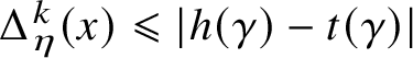 $\Delta _{\eta }^{k}(x)\leqslant |h(\gamma )-t(\gamma )|$
. Combined with the fact that intervals spanned by different k-solitons do not overlap (Lemma 1.5), this yields
$\Delta _{\eta }^{k}(x)\leqslant |h(\gamma )-t(\gamma )|$
. Combined with the fact that intervals spanned by different k-solitons do not overlap (Lemma 1.5), this yields
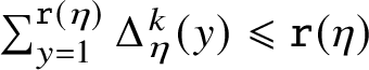 $\sum _{y=1}^{\mathtt r(\eta )} \Delta _{\eta }^k(y) \leqslant \mathtt r(\eta )$
, from which we get
$\sum _{y=1}^{\mathtt r(\eta )} \Delta _{\eta }^k(y) \leqslant \mathtt r(\eta )$
, from which we get
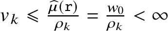 $v_k \leqslant \frac {\widehat {\mu }(\mathtt r)}{\rho _k} = \frac {w_0}{\rho _k} < \infty $
by (4.13).
$v_k \leqslant \frac {\widehat {\mu }(\mathtt r)}{\rho _k} = \frac {w_0}{\rho _k} < \infty $
by (4.13).
6.2 Equation for speeds from soliton interactions
We now prove that the soliton speeds satisfy (1.10). It is enough to consider
 $ k $
such that
$ k $
such that
 $ \rho _k>0 $
and otherwise take (1.10) as the definition of
$ \rho _k>0 $
and otherwise take (1.10) as the definition of
 $ v_k $
. We start by proving the following identity on the displacement of solitons.
$ v_k $
. We start by proving the following identity on the displacement of solitons.
Proposition 6.4. We have
 $$ \begin{align} x(\gamma^{t})-x(\gamma) = k\, t - 2k \sum_{m>k} \tfrac12 M_t^{\gamma}(m) + \sum_{m<k} 2m \, N_t^{\gamma}(m), \end{align} $$
where
 $$ \begin{align*} M_{t}^{\gamma}(m)&=\#\{(\tilde\gamma, s): \tilde\gamma\in \Gamma_{m}\eta, 0\leqslant s < t, I(\gamma^{s})\subseteq I(\tilde\gamma^{s}) \text{ and } x(\tilde\gamma^{s+1}) \ne x (\tilde\gamma^{s}) \}, \\ N_{t}^{\gamma}(m)&=\#\{(\tilde\gamma, s): \tilde\gamma\in \Gamma_{m}\eta, 0\leqslant s<t, I(\tilde\gamma^{s})\subseteq I(\gamma^{s}) \text{ and } I(\tilde\gamma^{s+1})\cap I(\gamma^{s+1})=\varnothing\}. \end{align*} $$
Proof. Before proving it, let us first explain the intuition underpinning (6.5). From Lemma 1.6, we know that as long as there exists some
 $\tilde \gamma $
satisfying
$\tilde \gamma $
satisfying
 $I(\gamma )\subseteq I(\tilde \gamma )$
,
$I(\gamma )\subseteq I(\tilde \gamma )$
,
 $\gamma $
is prevented from moving. We will see that it takes two time steps for
$\gamma $
is prevented from moving. We will see that it takes two time steps for
 $\tilde \gamma $
to overtake
$\tilde \gamma $
to overtake
 $\gamma $
: the first step occurs when
$\gamma $
: the first step occurs when
 $\gamma $
is nested in the right half of
$\gamma $
is nested in the right half of
 $\tilde {\gamma }$
, after which it will be nested in the left half of
$\tilde {\gamma }$
, after which it will be nested in the left half of
 $\tilde {\gamma }$
; the second step occurs when
$\tilde {\gamma }$
; the second step occurs when
 $\gamma $
is nested in the left half of
$\gamma $
is nested in the left half of
 $\tilde {\gamma }$
, after which it will no longer be nested inside
$\tilde {\gamma }$
, after which it will no longer be nested inside
 $\tilde {\gamma }$
. Because
$\tilde {\gamma }$
. Because
 $\tilde \gamma $
can be inside an even larger soliton, during which it stays frozen, these two times are not necessarily consecutive. On the other hand, when
$\tilde \gamma $
can be inside an even larger soliton, during which it stays frozen, these two times are not necessarily consecutive. On the other hand, when
 $\gamma $
overtakes a smaller soliton of size
$\gamma $
overtakes a smaller soliton of size
 $\ell $
say, it causes
$\ell $
say, it causes
 $\gamma $
to move
$\gamma $
to move
 $2\ell $
units more than it normally would have. Put formally, we have the following identity:
$2\ell $
units more than it normally would have. Put formally, we have the following identity:

The proof of this identity is elementary and is postponed to Section 7. Proceeding with the proof of (6.5), we note that if
 $\tilde \gamma $
exists in (6.6), then it has to be unique: solitons
$\tilde \gamma $
exists in (6.6), then it has to be unique: solitons
 $\tilde \gamma $
satisfying
$\tilde \gamma $
satisfying
 $I(\tilde \gamma )\supseteq I(\gamma )$
are ordered by their sizes and only the largest one will move forward. Iterating the above t times then yields (6.5).
$I(\tilde \gamma )\supseteq I(\gamma )$
are ordered by their sizes and only the largest one will move forward. Iterating the above t times then yields (6.5).
Now take
 $\tilde \gamma $
to be the leftmost m-soliton in
$\tilde \gamma $
to be the leftmost m-soliton in
 $[1, \infty )$
and
$[1, \infty )$
and
 $\gamma $
the rightmost k-soliton in
$\gamma $
the rightmost k-soliton in
 $(-\infty, 0]$
. We have shown previously that
$(-\infty, 0]$
. We have shown previously that
 $v_{m}=\lim _{t\to \infty } \frac {1}{t}x(\tilde \gamma ^{t})$
and
$v_{m}=\lim _{t\to \infty } \frac {1}{t}x(\tilde \gamma ^{t})$
and
 $v_{k}=\lim _{t\to \infty } \frac {1}{t}x(\gamma ^{t})$
,
$v_{k}=\lim _{t\to \infty } \frac {1}{t}x(\gamma ^{t})$
,
 $\mu $
-a.s. Combined with Lemma 1.7, this yields
$\mu $
-a.s. Combined with Lemma 1.7, this yields
 $$ \begin{align*} v_{k}\leqslant v_{m} \quad \text{if} \quad k<m \text{ and } \rho_{k}, \rho_{m}>0. \end{align*} $$
From now on, we will work under
 $\widehat {\mu }_{k}$
and always take
$\widehat {\mu }_{k}$
and always take
 $\gamma $
to be the soliton with
$\gamma $
to be the soliton with
 $x(\gamma )=0$
. To lighten the notation, we will drop the superscript
$x(\gamma )=0$
. To lighten the notation, we will drop the superscript
 ${\gamma }$
from
${\gamma }$
from
 $ M_t $
and
$ M_t $
and
 $ N_t $
. Recall that
$ N_t $
. Recall that
 $\bar {\rho }_m = \frac {\rho _m}{w_0}$
is the mean number of m-solitons per unit space.
$\bar {\rho }_m = \frac {\rho _m}{w_0}$
is the mean number of m-solitons per unit space.
Let us assume for the moment that
 $\bar {\rho }_m=0$
for all large m.
$\bar {\rho }_m=0$
for all large m.
By (1.9) and (6.5), to get (1.10) it suffices to show the following. For
 $m>k$
and
$m>k$
and
 $\ell <k$
:
$\ell <k$
:
 $$ \begin{align} \begin{aligned} \displaystyle \tfrac{1}{2t} M_t(m) &\to \bar{\rho}_m (v_m-v_k),\\ \tfrac{1}{t} N_t(\ell) &\to \bar{\rho}_\ell (v_k-v_\ell), \end{aligned} \qquad\qquad\text{ in probability}. \end{align} $$
Proof of (6.7)
Let us denote
 $\mathbf {M}_{t}(m)=\{(\tilde \gamma, s): \tilde \gamma \in \Gamma _{m}\eta, 0\leqslant s< t, I(\gamma ^{s})\subseteq I(\tilde \gamma ^{s}) \text { and } x(\tilde \gamma ^{s+1}) \ne x(\tilde \gamma ^{s}) \}$
, the set of solitons that overtake
$\mathbf {M}_{t}(m)=\{(\tilde \gamma, s): \tilde \gamma \in \Gamma _{m}\eta, 0\leqslant s< t, I(\gamma ^{s})\subseteq I(\tilde \gamma ^{s}) \text { and } x(\tilde \gamma ^{s+1}) \ne x(\tilde \gamma ^{s}) \}$
, the set of solitons that overtake
 $\gamma $
, so that
$\gamma $
, so that
 $M_{t}(m)=\#\mathbf {M}_{t}(m)$
. Let
$M_{t}(m)=\#\mathbf {M}_{t}(m)$
. Let
 $\gamma _{-}$
be the leftmost m-soliton satisfying
$\gamma _{-}$
be the leftmost m-soliton satisfying
 $x(\gamma _{-})> x(\gamma )$
and let
$x(\gamma _{-})> x(\gamma )$
and let
 $\gamma _{+}$
be the rightmost m-soliton satisfying
$\gamma _{+}$
be the rightmost m-soliton satisfying
 $x(\gamma _{+}) < x(\gamma )$
. Let us consider the m-solitons
$x(\gamma _{+}) < x(\gamma )$
. Let us consider the m-solitons
 $\tilde \gamma $
that are found between
$\tilde \gamma $
that are found between
 $\gamma ^{t}$
and
$\gamma ^{t}$
and
 $\gamma _{-}^{t}$
at time t and denote by
$\gamma _{-}^{t}$
at time t and denote by
 $\mathbf {L}^{-}_{t}$
their set, namely,
$\mathbf {L}^{-}_{t}$
their set, namely,
 $\mathbf {L}^{-}_{t} := \{ \tilde \gamma \in \Gamma _{m}\eta : x(\gamma ^{t}) < x(\tilde \gamma ^{t}) < x(\gamma _{-}^{t}) \}$
. Note that if
$\mathbf {L}^{-}_{t} := \{ \tilde \gamma \in \Gamma _{m}\eta : x(\gamma ^{t}) < x(\tilde \gamma ^{t}) < x(\gamma _{-}^{t}) \}$
. Note that if
 $\tilde \gamma \in \mathbf L^{-}_{t}$
, then necessarily
$\tilde \gamma \in \mathbf L^{-}_{t}$
, then necessarily
 $I(\gamma ^{t})\cap I(\tilde \gamma ^{t})=\varnothing $
. We also define
$I(\gamma ^{t})\cap I(\tilde \gamma ^{t})=\varnothing $
. We also define
 $\mathbf {L}^{+}_{t}=\{\tilde \gamma \in \Gamma _{m}\eta : I(\tilde \gamma ^{t})\cap [x(\gamma ^{t}), x(\gamma _{+}^{t})]\ne \varnothing \}$
, which includes in particular the m-soliton
$\mathbf {L}^{+}_{t}=\{\tilde \gamma \in \Gamma _{m}\eta : I(\tilde \gamma ^{t})\cap [x(\gamma ^{t}), x(\gamma _{+}^{t})]\ne \varnothing \}$
, which includes in particular the m-soliton
 $\tilde \gamma $
satisfying
$\tilde \gamma $
satisfying
 $I(\gamma ^{t})\subseteq I(\tilde \gamma ^{t})$
(if such a soliton exists). Roughly speaking,
$I(\gamma ^{t})\subseteq I(\tilde \gamma ^{t})$
(if such a soliton exists). Roughly speaking,
 $\#\mathbf {L}^{-}_{t}$
counts those m-solitons that have completed the 2-step overtaking of
$\#\mathbf {L}^{-}_{t}$
counts those m-solitons that have completed the 2-step overtaking of
 $\gamma $
between times
$\gamma $
between times
 $0$
and
$0$
and
 $t-1$
, so it will give an undercount of
$t-1$
, so it will give an undercount of
 $M_{t}(m)$
, whereas
$M_{t}(m)$
, whereas
 $\#\mathbf {L}^{+}_{t}$
will be an overcount. More precisely, let us show that
$\#\mathbf {L}^{+}_{t}$
will be an overcount. More precisely, let us show that
 $2\#\mathbf {L}^{-}_{t}\leqslant M_{t}(m)\leqslant 2 \#\mathbf {L}_{t}^{+}$
. Indeed, if
$2\#\mathbf {L}^{-}_{t}\leqslant M_{t}(m)\leqslant 2 \#\mathbf {L}_{t}^{+}$
. Indeed, if
 $(\tilde \gamma, s)\in \mathbf {M}_{t}(m)$
, then Lemma 1.7 implies that necessarily
$(\tilde \gamma, s)\in \mathbf {M}_{t}(m)$
, then Lemma 1.7 implies that necessarily
 $x(\tilde \gamma ) < x(\gamma )$
. It follows that
$x(\tilde \gamma ) < x(\gamma )$
. It follows that
 $x(\tilde \gamma )\leqslant x(\gamma _{+})$
, and then
$x(\tilde \gamma )\leqslant x(\gamma _{+})$
, and then
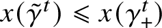 $x(\tilde \gamma ^{t})\leqslant x(\gamma _{+}^{t})$
. On the other hand, because
$x(\tilde \gamma ^{t})\leqslant x(\gamma _{+}^{t})$
. On the other hand, because
 $I(\gamma ^{s})\subseteq I(\tilde \gamma ^{s})$
, there are only two possibilities at
$I(\gamma ^{s})\subseteq I(\tilde \gamma ^{s})$
, there are only two possibilities at
 $s+1$
: either
$s+1$
: either
 $x(\tilde \gamma ^{s+1})> x(\gamma ^{s+1})$
(
$x(\tilde \gamma ^{s+1})> x(\gamma ^{s+1})$
(
 $\tilde \gamma $
overtakes
$\tilde \gamma $
overtakes
 $\gamma $
), which implies
$\gamma $
), which implies
 $x(\tilde \gamma ^{t})>x(\gamma ^{t})$
by Lemma 1.7, or
$x(\tilde \gamma ^{t})>x(\gamma ^{t})$
by Lemma 1.7, or
 $I(\gamma ^{s+1})\subseteq I(\tilde \gamma ^{s+1})$
. In the latter case, if
$I(\gamma ^{s+1})\subseteq I(\tilde \gamma ^{s+1})$
. In the latter case, if
 $s+1<t$
, we then repeat the arguments used for s; otherwise, we have
$s+1<t$
, we then repeat the arguments used for s; otherwise, we have
 $I(\gamma ^{t})\subseteq I(\tilde \gamma ^{t})$
. All cases considered, we conclude that
$I(\gamma ^{t})\subseteq I(\tilde \gamma ^{t})$
. All cases considered, we conclude that
 $\tilde \gamma \in \mathbf {L}^{+}_{t}$
. Moreover, for such a
$\tilde \gamma \in \mathbf {L}^{+}_{t}$
. Moreover, for such a
 $\tilde \gamma $
, there are at most two times s such that
$\tilde \gamma $
, there are at most two times s such that
 $(\tilde \gamma, s)\in \mathbf {M}_{t}(m)$
: the first time
$(\tilde \gamma, s)\in \mathbf {M}_{t}(m)$
: the first time
 $s'$
when
$s'$
when
 $I(\gamma ^{s})\subseteq I(\tilde \gamma ^{s})$
and
$I(\gamma ^{s})\subseteq I(\tilde \gamma ^{s})$
and
 $\tilde \gamma $
is the largest soliton containing
$\tilde \gamma $
is the largest soliton containing
 $\gamma $
(i.e., first step in overtaking) and the first time
$\gamma $
(i.e., first step in overtaking) and the first time
 $s''$
after
$s''$
after
 $s'$
when
$s'$
when
 $\tilde \gamma $
moves forward (i.e., second step in overtaking). And for all
$\tilde \gamma $
moves forward (i.e., second step in overtaking). And for all
 $u\geqslant s''+1$
, we have
$u\geqslant s''+1$
, we have
 $x(\tilde \gamma ^{u})> x(\gamma ^{u})$
as implied by Lemmas 1.6 and 1.7, so that
$x(\tilde \gamma ^{u})> x(\gamma ^{u})$
as implied by Lemmas 1.6 and 1.7, so that
 $\gamma $
and
$\gamma $
and
 $\tilde \gamma $
will never intersect again. Because
$\tilde \gamma $
will never intersect again. Because
 $s'$
and
$s'$
and
 $s''$
do not necessarily belong to
$s''$
do not necessarily belong to
 $[0, t)$
, we only have
$[0, t)$
, we only have
 $M_{t}(m)\leqslant 2 \#\mathbf {L}_{t}^{+}$
. For the other inequality, we note that if
$M_{t}(m)\leqslant 2 \#\mathbf {L}_{t}^{+}$
. For the other inequality, we note that if
 $\tilde \gamma \in \mathbf {L}^{-}_{t}$
, then
$\tilde \gamma \in \mathbf {L}^{-}_{t}$
, then
 $x(\tilde \gamma )< x(\gamma _{-})$
, which implies actually
$x(\tilde \gamma )< x(\gamma _{-})$
, which implies actually
 $x(\tilde \gamma )\leqslant x(\gamma _{+})<x(\gamma )$
. Because
$x(\tilde \gamma )\leqslant x(\gamma _{+})<x(\gamma )$
. Because
 $x(\tilde \gamma ^{t})> x(\gamma ^{t})$
, it follows that both
$x(\tilde \gamma ^{t})> x(\gamma ^{t})$
, it follows that both
 $s' $
and
$s' $
and
 $ s'' $
described previously belong to
$ s'' $
described previously belong to
 $[0, t)$
. So the claimed inequalities follow.
$[0, t)$
. So the claimed inequalities follow.
Write whp to denote ‘with high
 $ \widehat {\mu }_k $
-probability’ and note that high
$ \widehat {\mu }_k $
-probability’ and note that high
 $ \mu $
implies high
$ \mu $
implies high
 $ \widehat {\mu }_k $
. By (1.9), for every
$ \widehat {\mu }_k $
. By (1.9), for every
 $ \varepsilon>0 $
,
$ \varepsilon>0 $
,
 $ x(\gamma ^t) $
is in
$ x(\gamma ^t) $
is in
 $ v_k t \pm \varepsilon t $
and
$ v_k t \pm \varepsilon t $
and
 $ x(\gamma _-^t) $
is in
$ x(\gamma _-^t) $
is in
 $ v_m t \pm \varepsilon t $
whp. Using
$ v_m t \pm \varepsilon t $
whp. Using
 $ \theta $
-invariance of
$ \theta $
-invariance of
 $ \mu $
, by the ergodic theorem applied to counting
$ \mu $
, by the ergodic theorem applied to counting
 $ m $
-solitons on a large interval, the number of
$ m $
-solitons on a large interval, the number of
 $ m $
-solitons of
$ m $
-solitons of
 $ T^t \eta $
located in
$ T^t \eta $
located in
 $ [v_k t \pm \varepsilon t, v_m t \pm \varepsilon t ] $
is within
$ [v_k t \pm \varepsilon t, v_m t \pm \varepsilon t ] $
is within
 $ \bar {\rho }_k(v_m-v_k)t \pm 3\varepsilon t $
whp. Therefore,
$ \bar {\rho }_k(v_m-v_k)t \pm 3\varepsilon t $
whp. Therefore,
 $ \# \mathbf {L}_t^- $
is in
$ \# \mathbf {L}_t^- $
is in
 $ \bar {\rho }_m (v_m-v_k)t \pm 3\varepsilon t $
whp. Because
$ \bar {\rho }_m (v_m-v_k)t \pm 3\varepsilon t $
whp. Because
 $ \mathbf {L}_t^+ $
and
$ \mathbf {L}_t^+ $
and
 $ \mathbf {L}_t^- $
can differ by at most two
$ \mathbf {L}_t^- $
can differ by at most two
 $ m $
-solitons, this concludes the proof that
$ m $
-solitons, this concludes the proof that
 $ \tfrac {1}{2t} M_t(m) \to \bar {\rho }_m (v_m-v_k) $
in probability.
$ \tfrac {1}{2t} M_t(m) \to \bar {\rho }_m (v_m-v_k) $
in probability.
The proof for
 $N_{t}(\ell )$
is similar but simpler. The only difference is that for each
$N_{t}(\ell )$
is similar but simpler. The only difference is that for each
 $\tilde \gamma \in \Gamma _{\ell }\eta $
, there is at most one time s such that
$\tilde \gamma \in \Gamma _{\ell }\eta $
, there is at most one time s such that
 $(\tilde \gamma, s)$
is counted in the tally
$(\tilde \gamma, s)$
is counted in the tally
 $N_{t}(\ell )$
.
$N_{t}(\ell )$
.
To complete the proof of (1.10), it remains to drop the assumption that
 $\bar {\rho }_m=0$
for all large m. The above proof contains all of the argument, except that combining (6.5) and (6.7) requires a limit and an infinite sum to commute. To prove the general case, we take expectation in (6.5) with
$\bar {\rho }_m=0$
for all large m. The above proof contains all of the argument, except that combining (6.5) and (6.7) requires a limit and an infinite sum to commute. To prove the general case, we take expectation in (6.5) with
 $t=1$
and combine it with (6.1):
$t=1$
and combine it with (6.1):
 $$ \begin{align*} v_k &= \int x(\gamma^1) \widehat{\mu}_k (\mathrm{d} \eta) = \int \Big[ k - \sum_{m>k} k\,M_1(m) + \sum_{m < k}2m\, N_1(m) \Big] \, \widehat{\mu}_k(\mathrm{d} \eta)\\ & = k - k\sum_{m> k} \int M_{1}(m) \widehat{\mu}_{k}(\mathrm{d}\eta)+ \sum_{m<k}2m \int N_1(m) \, \widehat{\mu}_k(\mathrm{d} \eta). \end{align*} $$
It remains to show
 $\int N_1(m) \, \widehat {\mu }_k(\mathrm {d} \eta ) = \bar {\rho }_m(v_k-v_m)$
and
$\int N_1(m) \, \widehat {\mu }_k(\mathrm {d} \eta ) = \bar {\rho }_m(v_k-v_m)$
and
 $\frac 12\int M_1(m) \, \widehat {\mu }_k(\mathrm {d} \eta ) = \bar {\rho }_m(v_m-v_k)$
. Similar to the argument in Subsection 6.1, we decompose
$\frac 12\int M_1(m) \, \widehat {\mu }_k(\mathrm {d} \eta ) = \bar {\rho }_m(v_m-v_k)$
. Similar to the argument in Subsection 6.1, we decompose
 $$ \begin{align*} N_{t+1}(m) = N^{\eta}_{1}(m) + N_1^{\widehat{T}_k \eta}(m) + N_1^{\widehat{T}_k^2 \eta}(m) + \dots + N_1^{\widehat{T}_k^t \eta}(m) \end{align*} $$
with a slight abuse of notation. By
 $\widehat {T}_k$
-invariance,
$\widehat {T}_k$
-invariance,
 $\frac {1}{t}N_t^{\eta }(m)$
converges
$\frac {1}{t}N_t^{\eta }(m)$
converges
 $\widehat {\mu }_k$
-a.s. to a random variable (i.e., a measurable function of
$\widehat {\mu }_k$
-a.s. to a random variable (i.e., a measurable function of
 $\eta $
) whose average is
$\eta $
) whose average is
 $\int N_1^{\eta }(m) \, \widehat {\mu }_k(\mathrm {d} \eta )$
. On the other hand, by (6.7) this variable is constant and equal to
$\int N_1^{\eta }(m) \, \widehat {\mu }_k(\mathrm {d} \eta )$
. On the other hand, by (6.7) this variable is constant and equal to
 $\bar {\rho }_m|v_k-v_m|$
. The same argument works for
$\bar {\rho }_m|v_k-v_m|$
. The same argument works for
 $M_{1}(m)$
. This concludes the proof of (1.10) and also of Theorem 1.1.
$M_{1}(m)$
. This concludes the proof of (1.10) and also of Theorem 1.1.
6.3 Soliton speeds are positive and increasing
Here we show that
 $ v_k $
is positive and increasing in
$ v_k $
is positive and increasing in
 $ k $
without assuming that
$ k $
without assuming that
 $ \bar {\rho }_k>0 $
. Both follow from combining (1.10) with the following bound on the total flow of solitons crossing the origin:
$ \bar {\rho }_k>0 $
. Both follow from combining (1.10) with the following bound on the total flow of solitons crossing the origin:
 $$ \begin{align} 2 \bar{\rho} \cdot v := 2 \sum_m \bar{\rho}_m v_m < 1. \end{align} $$
The idea is that
 $ \rho _m v_m $
is the average flow of solitons through the origin and each one takes two time steps. Before sketching the proof, we show that soliton speeds are positive and increasing.
$ \rho _m v_m $
is the average flow of solitons through the origin and each one takes two time steps. Before sketching the proof, we show that soliton speeds are positive and increasing.
Splitting and regrouping the sums in (1.10) gives
 $$ \begin{align*} v_k = k - \sum_{m} 2 (k \wedge m) \bar{\rho}_m v_m + v_k \, \sum_{m} 2 (k \wedge m) \bar{\rho}_m = a v_k + b, \end{align*} $$
where
 $ a \leqslant 2\lambda <1 $
and
$ a \leqslant 2\lambda <1 $
and
 $ b \geqslant k - 2k \bar {\rho } \cdot v>0 $
. Hence,
$ b \geqslant k - 2k \bar {\rho } \cdot v>0 $
. Hence,
 $ v_k>0 $
.
$ v_k>0 $
.
Now, writing
 $ d_k := v_{k+1}-v_k> 0 $
, by subtracting the above equation from itself we get
$ d_k := v_{k+1}-v_k> 0 $
, by subtracting the above equation from itself we get
 $$ \begin{align*} d_k &= 1 + d_k \sum_{m} 2 (k \wedge m) \bar{\rho}_m + \sum_{m \geqslant k+1} 2 \bar{\rho}_m (v_{k+1}-v_m) = a d_k + b + c, \end{align*} $$
where
 $ a \leqslant 2 \lambda < 1 $
,
$ a \leqslant 2 \lambda < 1 $
,
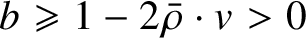 $ b \geqslant 1 - 2\bar {\rho }\cdot v> 0 $
and
$ b \geqslant 1 - 2\bar {\rho }\cdot v> 0 $
and
 $ c = \sum _{m>k}2 \bar {\rho }_m v_{k+1} \geqslant 0 $
. Therefore,
$ c = \sum _{m>k}2 \bar {\rho }_m v_{k+1} \geqslant 0 $
. Therefore,
 $ d_k>0 $
.
$ d_k>0 $
.
Proof of (6.8). The proof bears much similarity to that of (6.7), so we only sketch the arguments here. Denote by
 $Q_{t}(k)=\#\{(\gamma, s): \gamma \in \Gamma _{k}\eta, 0\leqslant s<t, 0\in I(\gamma ^{s}) \text { and } x(\gamma ^{s+1})\ne x(\gamma ^{s})\}$
the number of occurrences that a k-soliton is the largest one straddling
$Q_{t}(k)=\#\{(\gamma, s): \gamma \in \Gamma _{k}\eta, 0\leqslant s<t, 0\in I(\gamma ^{s}) \text { and } x(\gamma ^{s+1})\ne x(\gamma ^{s})\}$
the number of occurrences that a k-soliton is the largest one straddling
 $0$
between times
$0$
between times
 $0$
and t. Note that each
$0$
and t. Note that each
 $ k $
-soliton that crosses the origin in the time interval
$ k $
-soliton that crosses the origin in the time interval
 $[0,t]$
contributes twice to
$[0,t]$
contributes twice to
 $Q_{t}(k)$
, once when the origin is in its tail and once in its head.
$Q_{t}(k)$
, once when the origin is in its tail and once in its head.
To find the growth rate of
 $Q_{t}(k)$
as
$Q_{t}(k)$
as
 $ t\to \infty $
, let us denote by
$ t\to \infty $
, let us denote by
 $\gamma _{+}$
the rightmost k-soliton
$\gamma _{+}$
the rightmost k-soliton
 $\gamma '$
satisfying
$\gamma '$
satisfying
 $x(\gamma ')\leqslant 0$
. The counts
$x(\gamma ')\leqslant 0$
. The counts
 $Q^{-}_{t}(k) = 2\#\{\gamma \in \Gamma _{k}\eta : 0<x(\gamma ^{t})<x(\gamma _{+}^{t})\}$
and
$Q^{-}_{t}(k) = 2\#\{\gamma \in \Gamma _{k}\eta : 0<x(\gamma ^{t})<x(\gamma _{+}^{t})\}$
and
 $Q^{+}_{t}(k) = 2\#\{\gamma \in \Gamma _{k}\eta : I(\gamma ^{t})\cap [0, x(\gamma _{+}^{t})]\ne \varnothing \}$
satisfy
$Q^{+}_{t}(k) = 2\#\{\gamma \in \Gamma _{k}\eta : I(\gamma ^{t})\cap [0, x(\gamma _{+}^{t})]\ne \varnothing \}$
satisfy
 $Q^{-}_{t}(k)-3 \leqslant Q_{t}(k) \leqslant Q^{+}_{t}(k)$
. Arguments identical to those in (6.7) show that
$Q^{-}_{t}(k)-3 \leqslant Q_{t}(k) \leqslant Q^{+}_{t}(k)$
. Arguments identical to those in (6.7) show that
 $\frac {1}{t}Q_{t}(k)\to 2\bar {\rho }_{k}v_{k}$
in probability for each
$\frac {1}{t}Q_{t}(k)\to 2\bar {\rho }_{k}v_{k}$
in probability for each
 $k\geqslant 1$
.
$k\geqslant 1$
.
Applying the ergodic theorem for
 $ T $
, convergence of
$ T $
, convergence of
 $\frac {1}{t}Q_{t}(k)$
says that
$\frac {1}{t}Q_{t}(k)$
says that
 $ 2 \bar {\rho }_k v_k $
equals the probability that the largest soliton
$ 2 \bar {\rho }_k v_k $
equals the probability that the largest soliton
 $ \gamma $
such that
$ \gamma $
such that
 $ 0\in I(\gamma ) $
belongs to
$ 0\in I(\gamma ) $
belongs to
 $\Gamma _k \eta $
. For each
$\Gamma _k \eta $
. For each
 $ \eta \in \mathcal {X} $
, either
$ \eta \in \mathcal {X} $
, either
 $ 0\in R\eta $
or there is a unique such
$ 0\in R\eta $
or there is a unique such
 $ k $
, so
$ k $
, so
 $$ \begin{align*} \mu(0\in R\eta) + \sum_k 2 \bar{\rho}_k v_k = 1, \end{align*} $$
concluding the proof.
6.4 Recursion formulas for independent components
We now prove Theorem 1.2. Let
 $\zeta = M \eta $
. We are assuming that the field
$\zeta = M \eta $
. We are assuming that the field
 $\left ( \zeta _k(i) \right )_{i\in \mathbb {Z}}$
is i.i.d. over i for each k and independent over k. So let us proceed the other way around. We let P denote the law of
$\left ( \zeta _k(i) \right )_{i\in \mathbb {Z}}$
is i.i.d. over i for each k and independent over k. So let us proceed the other way around. We let P denote the law of
 $\zeta $
and E the corresponding expectation. In this notation,
$\zeta $
and E the corresponding expectation. In this notation,
 $\widehat {\mu }$
is the law of
$\widehat {\mu }$
is the law of
 $\eta =M^{-1} \zeta $
.
$\eta =M^{-1} \zeta $
.
Note that (4.11) and (4.12) give the first two equations in (1.12). The third equation can be taken as the definition of
 $s_k$
, and it is a simple recursive definition once one has
$s_k$
, and it is a simple recursive definition once one has
 $\rho $
, w and
$\rho $
, w and
 $\alpha $
. Combining these with (6.3), to get the last equation in (1.12) we need to show that
$\alpha $
. Combining these with (6.3), to get the last equation in (1.12) we need to show that
 $$ \begin{align} E \sum_{y=0}^{\mathtt r(\eta)-1} \Delta^k_\eta(y) = \alpha_k \cdot s_k. \end{align} $$
We now use the assumption that
 $\eta =M^{-1} \zeta $
, where
$\eta =M^{-1} \zeta $
, where
 $M^{-1}$
denotes de reconstruction map of Subsection 2.2. First, note that
$M^{-1}$
denotes de reconstruction map of Subsection 2.2. First, note that
 $$ \begin{align*}\sum_{y=0}^{\mathtt r(\eta)-1} \Delta^k_\eta(y) = \sum_\gamma x(\gamma_1)-x(\gamma),\end{align*} $$
where the sum is over all
 $ k $
-solitons
$ k $
-solitons
 $ \gamma $
located between record 0 and record 1. Moreover, k-solitons appended to k-slots belonging to larger solitons will stay put, just switching zeros for ones, and only the k-solitons that are appended directly to the
$ \gamma $
located between record 0 and record 1. Moreover, k-solitons appended to k-slots belonging to larger solitons will stay put, just switching zeros for ones, and only the k-solitons that are appended directly to the
 $0$
th k-slot at
$0$
th k-slot at
 $x=0$
will actually jump (Lemma 1.6). Furthermore, by Proposition 1.3 and Lemma 1.6, the size of their jump equals the distance between their leftmost
$x=0$
will actually jump (Lemma 1.6). Furthermore, by Proposition 1.3 and Lemma 1.6, the size of their jump equals the distance between their leftmost
 $ 1 $
and their leftmost
$ 1 $
and their leftmost
 $ 0 $
; that is, the distance between the tip of their head and the tip of their tail.
$ 0 $
; that is, the distance between the tip of their head and the tip of their tail.
Now the number of k-solitons appended to the
 $0$
th k-slot is exactly
$0$
th k-slot is exactly
 $\zeta _k(0)$
, which on average equals
$\zeta _k(0)$
, which on average equals
 $\alpha _k$
by (4.10). So to conclude the proof of (6.9), it is enough to observe that
$\alpha _k$
by (4.10). So to conclude the proof of (6.9), it is enough to observe that
 $s_k$
given by the recursion relation in (1.12) in fact gives the expected distance between the tips of the head and tail of a typical k-soliton appended to a record. By independence of
$s_k$
given by the recursion relation in (1.12) in fact gives the expected distance between the tips of the head and tail of a typical k-soliton appended to a record. By independence of
 $ \zeta _k $
over
$ \zeta _k $
over
 $ k $
, being appended to a record is irrelevant, and we can consider a typical
$ k $
, being appended to a record is irrelevant, and we can consider a typical
 $ k $
-soliton instead.
$ k $
-soliton instead.
We claim that
 $ s_k $
equals the a.s. empirical average of the distance between the tip of the head and the tip of the tail among all
$ s_k $
equals the a.s. empirical average of the distance between the tip of the head and the tip of the tail among all
 $ k $
-solitons and also that
$ k $
-solitons and also that
 $ 2s_k $
equals the a.s. empirical average of the size of
$ 2s_k $
equals the a.s. empirical average of the size of
 $ I(\gamma ) $
among all
$ I(\gamma ) $
among all
 $ k $
-solitons
$ k $
-solitons
 $ \gamma $
. We made the previous statement stronger so we can prove it by induction. Remember that the interval
$ \gamma $
. We made the previous statement stronger so we can prove it by induction. Remember that the interval
 $ I(\gamma ) $
consists of sites occupied by
$ I(\gamma ) $
consists of sites occupied by
 $ \gamma $
together with the smaller solitons appended to its slots. For
$ \gamma $
together with the smaller solitons appended to its slots. For
 $k=1$
we have
$k=1$
we have
 $s_1=1$
, consistent with the fact that a
$s_1=1$
, consistent with the fact that a
 $1$
-soliton is always given by the strings
$1$
-soliton is always given by the strings
 $a=10$
or
$a=10$
or
 $\tilde {a}=01$
with nothing appended inside it. For
$\tilde {a}=01$
with nothing appended inside it. For
 $k=2$
, note that each
$k=2$
, note that each
 $2$
-soliton (including smaller solitons appended to its slots) is of the form
$2$
-soliton (including smaller solitons appended to its slots) is of the form
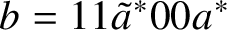 $b=11\tilde {a}^*00{a}^*$
or
$b=11\tilde {a}^*00{a}^*$
or
 $\tilde {b}=00{a}^*11\tilde {a}^*$
where
$\tilde {b}=00{a}^*11\tilde {a}^*$
where
 $a^*$
stands for
$a^*$
stands for
 $\zeta _1(i)$
copies of a and
$\zeta _1(i)$
copies of a and
 $\tilde {a}^*$
stands for
$\tilde {a}^*$
stands for
 $\zeta _1(j)$
copies of
$\zeta _1(j)$
copies of
 $\tilde {a}$
for some
$\tilde {a}$
for some
 $i,j$
that are determined by
$i,j$
that are determined by
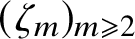 $(\zeta _m)_{m\geqslant 2}$
. So the average size of
$(\zeta _m)_{m\geqslant 2}$
. So the average size of
 $11\tilde {a}^*$
and that of
$11\tilde {a}^*$
and that of
 $00a^*$
both equal
$00a^*$
both equal
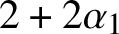 $2+2\alpha _1$
. For
$2+2\alpha _1$
. For
 $k=3$
, note that each
$k=3$
, note that each
 $3$
-soliton is of the form
$3$
-soliton is of the form
 ${c}=11\tilde {a}^*1\tilde {a}^*\tilde {b}^*00{a}^*0{a}^*{b}^*$
or
${c}=11\tilde {a}^*1\tilde {a}^*\tilde {b}^*00{a}^*0{a}^*{b}^*$
or
 $\tilde {c}=00{a}^*0{a}^*{b}^*11\tilde {a}^*1\tilde {a}^*\tilde {b}^*$
where
$\tilde {c}=00{a}^*0{a}^*{b}^*11\tilde {a}^*1\tilde {a}^*\tilde {b}^*$
where
 $b^*$
stands for
$b^*$
stands for
 $\zeta _2(i)$
independent copies of b, etc. So the average size of each half of a
$\zeta _2(i)$
independent copies of b, etc. So the average size of each half of a
 $3$
-soliton equals
$3$
-soliton equals
 $s_3=3 + 2s_2 \alpha _2 + 4 s_1 \alpha _1$
. The induction step is clear, which concludes the proof of Theorem 1.2.
$s_3=3 + 2s_2 \alpha _2 + 4 s_1 \alpha _1$
. The induction step is clear, which concludes the proof of Theorem 1.2.
6.5 Vertical speed
A previous version of this work [arXiv:1806.02798v3] focussed on measuring vertical speed of solitons, before the authors realised that it was in fact possible to study the horizontal speeds.
We now briefly mention the results about vertical speed. The analysis is very similar to what was done in Subsection 6.2, and tedious details will be omitted.
For
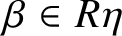 $\beta \in R\eta $
, we define
$\beta \in R\eta $
, we define
 $\beta$
t
:= r(T
t
$\beta$
t
:= r(T
t
 $\xi$
, j), where
$\xi$
, j), where
 $\beta$
= r(
$\beta$
= r(
 $\xi$
, j). Note that this definition does not depend on the lift
$\xi$
, j). Note that this definition does not depend on the lift
 $\xi [\eta ]$
. Recalling (3.2), we define the displacement of a k-bearer
$\xi [\eta ]$
. Recalling (3.2), we define the displacement of a k-bearer
 $\pi \in S_k\eta $
measured in terms of records by
$\pi \in S_k\eta $
measured in terms of records by
 $$ \begin{align*} y_k^t(\eta,\pi) = \# \left\{ \beta\in R\eta: \pi < \beta \text{ and } \pi^{k,t} \geqslant \beta^t \right\}, \quad \pi \in S_k \eta. \end{align*} $$
In case there is a k-soliton
 $\gamma \in \Gamma _k\eta $
appended to the k-slot
$\gamma \in \Gamma _k\eta $
appended to the k-slot
 $\pi $
in
$\pi $
in
 $\eta $
, the tagged k-soliton
$\eta $
, the tagged k-soliton
 $\gamma ^t$
will appear appended to the k-slot
$\gamma ^t$
will appear appended to the k-slot
 $\pi ^{k,t}$
in
$\pi ^{k,t}$
in
 $T^t\eta $
, so
$T^t\eta $
, so
 $y_k^t$
also measures the displacement of tagged k-solitons, but it is well defined even when there are no k-solitons. The limit (6.13) gives a physical meaning to the soliton speeds
$y_k^t$
also measures the displacement of tagged k-solitons, but it is well defined even when there are no k-solitons. The limit (6.13) gives a physical meaning to the soliton speeds
 $v_k$
when
$v_k$
when
 $\rho _k=0$
in Theorem 1.1.
$\rho _k=0$
in Theorem 1.1.
Theorem 6.1. Let
 $\mu $
be a measure on
$\mu $
be a measure on
 $\mathcal {X}$
such that under
$\mathcal {X}$
such that under
 $\widehat {\mu }$
each kth component
$\widehat {\mu }$
each kth component
 $M_k \eta $
is i.i.d. and they are independent over k. There exists a nondecreasing deterministic sequence
$M_k \eta $
is i.i.d. and they are independent over k. There exists a nondecreasing deterministic sequence
 $h=(h_k)_{k\geqslant 1}$
such that
$h=(h_k)_{k\geqslant 1}$
such that
 $\mu $
-a.s. on
$\mu $
-a.s. on
 $\eta $
, for all
$\eta $
, for all
 $k\in \mathbb {N}$
and
$k\in \mathbb {N}$
and
 $\pi \in S_k\eta $
,
$\pi \in S_k\eta $
,
 $$ \begin{align} \lim_{t\to\infty} \frac{y_k^t(\eta,\pi)}{t} &= h_k \in [k,\infty]. \end{align} $$
Assuming
 $\sum$
k
k
2
$\sum$
k
k
2
 $\rho$
k
$\rho$
k
 $< \infty$
, the vector
$< \infty$
, the vector
 $(h_k)_{k\geqslant 1}$
is the unique finite solution of the linear system
$(h_k)_{k\geqslant 1}$
is the unique finite solution of the linear system
 $$ \begin{align} h_k &= k + \sum_{m>k} 2(m-k)(h_m-h_k)\rho_m,\quad k\geqslant 1. \end{align} $$
The asymptotic speed of tagged records is given by
 $$ \begin{align} \lim_{t\to\infty} - \frac{\beta^t}{t} = v_0 := \sum_{m\geqslant 1} 2m \rho_m h_m, \quad \text{for all } \beta\in R\eta,\ \mu\text{-a.s.} \end{align} $$
The asymptotic speed
 $v_k$
of k-bearers is also given by
$v_k$
of k-bearers is also given by
 $$ \begin{align} \lim_{t\to\infty} \frac{\pi^{k,t}}{t} = v_k = h_k w_0 - v_0,\quad \text{ for all } \pi\in S_k\eta,\ \mu\text{-a.s.}, \end{align} $$
From the two last equations, the speed of tagged records is also given by
 $$ \begin{align} v_0=\sum_{m\geqslant 1} 2m \rho_m v_m. \end{align} $$
Furthermore, the vertical speed of any walk representation
 $\xi =\xi [\eta ]$
is given by
$\xi =\xi [\eta ]$
is given by
 $$ \begin{align} \lim_{t\to\infty} -\frac{T^t\xi(0)}{t} = h_0 := \frac{v_0}{w_0}. \end{align} $$
Let us outline the argument for the first four equations.
The proof of (6.10) is similar to that of (1.9) and only uses
 $ \theta $
-ergodicity of
$ \theta $
-ergodicity of
 $ \eta $
. Each time an m-soliton overtakes a k-bearer, this causes the position of the k-bearer measured in records to be incremented by an extra factor of
$ \eta $
. Each time an m-soliton overtakes a k-bearer, this causes the position of the k-bearer measured in records to be incremented by an extra factor of
 $2(m-k)$
. On the other hand, the position of a
$2(m-k)$
. On the other hand, the position of a
 $ k $
-bearer measured in records is not affected by overtaking smaller solitons. These two facts explain the origin of (6.11), but the proof uses a truncation argument that deletes all large components, and the i.i.d. assumption is to ensure that the resulting configuration is still
$ k $
-bearer measured in records is not affected by overtaking smaller solitons. These two facts explain the origin of (6.11), but the proof uses a truncation argument that deletes all large components, and the i.i.d. assumption is to ensure that the resulting configuration is still
 $ \theta $
-ergodic.
$ \theta $
-ergodic.
The speeds
 $ h_k $
are either all finite or all infinite; they are finite if and only if
$ h_k $
are either all finite or all infinite; they are finite if and only if
 $ \sum _m m^2 \rho _m < \infty $
. Deleting large solitons, one gets from (6.11) that
$ \sum _m m^2 \rho _m < \infty $
. Deleting large solitons, one gets from (6.11) that
 $ 0 \leqslant h_m - h_k \leqslant m-k $
. Plugging this back into (6.11) and using
$ 0 \leqslant h_m - h_k \leqslant m-k $
. Plugging this back into (6.11) and using
 $ \sum _m m \rho _m < \infty $
, one eventually gets
$ \sum _m m \rho _m < \infty $
, one eventually gets
 $ h_{k+j} - h_k \geqslant \delta j $
for some
$ h_{k+j} - h_k \geqslant \delta j $
for some
 $ \delta>0 $
and all large
$ \delta>0 $
and all large
 $ k $
. This gives
$ k $
. This gives
 $ \delta k \leqslant h_k \leqslant k + 2 \sum _m m^2 \rho _m $
uniformly with respect to the deletion threshold, which yields stated equivalence. Also, under this condition, one can show existence and uniqueness of the solution to (6.11) using truncation, as we did for (4.11).
$ \delta k \leqslant h_k \leqslant k + 2 \sum _m m^2 \rho _m $
uniformly with respect to the deletion threshold, which yields stated equivalence. Also, under this condition, one can show existence and uniqueness of the solution to (6.11) using truncation, as we did for (4.11).
Each time a tagged m-soliton crosses a tagged record from left to right, it causes the record to move
 $2m$
boxes left. On the other hand, by mass conservation the number of such crossings by time t equals
$2m$
boxes left. On the other hand, by mass conservation the number of such crossings by time t equals
 $\rho _m y_m^t$
, which is about
$\rho _m y_m^t$
, which is about
 $\rho _m h_m t$
by (6.10). Summing over m we get (6.12). As a side remark, the vertical speed
$\rho _m h_m t$
by (6.10). Summing over m we get (6.12). As a side remark, the vertical speed
 $h_0$
is given by the expected vertical jump at the origin
$h_0$
is given by the expected vertical jump at the origin
 $h_0 = \int (\xi [\eta ](0)-T\xi [\eta ](0)) \mu (\mathrm {d}\eta )$
, and intuitively this is related to
$h_0 = \int (\xi [\eta ](0)-T\xi [\eta ](0)) \mu (\mathrm {d}\eta )$
, and intuitively this is related to
 $ \sum _k k^2 \rho _k $
because the excursion contained the origin is size-biased.
$ \sum _k k^2 \rho _k $
because the excursion contained the origin is size-biased.
Finally, by (6.10), the k-bearer
 $\pi = 0 \in S_k \xi $
will typically have crossed about
$\pi = 0 \in S_k \xi $
will typically have crossed about
 $h_k t$
records by time t, so it will be between two tagged records with initial index about
$h_k t$
records by time t, so it will be between two tagged records with initial index about
 $h_k t$
. By ergodicity, the initial position of these records is about
$h_k t$
. By ergodicity, the initial position of these records is about
 $w_0 h_k t$
, so by (6.12) their position at time t will be about
$w_0 h_k t$
, so by (6.12) their position at time t will be about
 $w_0 h_k t - v_0 t$
. Dividing by t and taking a limit, one gets (6.13).
$w_0 h_k t - v_0 t$
. Dividing by t and taking a limit, one gets (6.13).
From (6.13) we have
 $h_m = \frac {v_0+v_m}{w_0}$
, and substituting into (6.12) and using (4.13) we get (6.14). To prove (6.15), we note that after t iterations of T, record i will be at
$h_m = \frac {v_0+v_m}{w_0}$
, and substituting into (6.12) and using (4.13) we get (6.14). To prove (6.15), we note that after t iterations of T, record i will be at
 $x=o(t)$
if
$x=o(t)$
if
 $r(\xi,i) = v_0 t + o(t)$
, which implies that
$r(\xi,i) = v_0 t + o(t)$
, which implies that
 $T^t \xi (0) = -i + o(t)$
. On the other hand,
$T^t \xi (0) = -i + o(t)$
. On the other hand,
 $r(\xi,i) = w_0 i + o(i)$
, whence
$r(\xi,i) = w_0 i + o(i)$
, whence
 $T^t \xi (0) = -h_0 t + o(t)$
, concluding the proof.
$T^t \xi (0) = -h_0 t + o(t)$
, concluding the proof.
7 Postponed proofs
Proof of Proposition 1.3. Let us prove for finite
 $\eta $
first. The proof is by induction on number of balls contained in
$\eta $
first. The proof is by induction on number of balls contained in
 $\eta $
. Identifying
$\eta $
. Identifying
 $0$
with ‘
$0$
with ‘
 $\ominus $
’ and
$\ominus $
’ and
 $1$
with ‘
$1$
with ‘
 $\oplus $
’, consider the following data stream version of the TS-Algorithm.
$\oplus $
’, consider the following data stream version of the TS-Algorithm.

For example, for the finite sequence
 $\eta =\oplus \oplus \ominus \oplus \oplus \ominus \ominus \oplus \oplus \oplus \ominus \ominus \ominus \ominus \ominus $
the algorithm would produce the words
$\eta =\oplus \oplus \ominus \oplus \oplus \ominus \ominus \oplus \oplus \oplus \ominus \ominus \ominus \ominus \ominus $
the algorithm would produce the words
 $\ominus ^{\infty }\oplus $
,
$\ominus ^{\infty }\oplus $
,
 $\ominus ^{\infty }\oplus ^2$
,
$\ominus ^{\infty }\oplus ^2$
,
 $\ominus ^{\infty }\oplus ^2\ominus $
,
$\ominus ^{\infty }\oplus ^2\ominus $
,
 $\ominus ^{\infty }\oplus ^2\underline {\ominus \oplus }$
,
$\ominus ^{\infty }\oplus ^2\underline {\ominus \oplus }$
,
 $\ominus ^{\infty }\oplus ^3$
,
$\ominus ^{\infty }\oplus ^3$
,
 $\ominus ^{\infty }\oplus ^3\ominus $
,
$\ominus ^{\infty }\oplus ^3\ominus $
,
 $\ominus ^{\infty }\oplus ^3\ominus ^2$
,
$\ominus ^{\infty }\oplus ^3\ominus ^2$
,
 $\ominus ^{\infty }\oplus ^3\ominus ^2\oplus $
,
$\ominus ^{\infty }\oplus ^3\ominus ^2\oplus $
,
 $\ominus ^{\infty }\oplus ^3\underline {\ominus ^2\oplus ^2}$
,
$\ominus ^{\infty }\oplus ^3\underline {\ominus ^2\oplus ^2}$
,
 $\ominus ^{\infty }\oplus ^4$
,
$\ominus ^{\infty }\oplus ^4$
,
 $\ominus ^{\infty }\oplus ^4\ominus $
,
$\ominus ^{\infty }\oplus ^4\ominus $
,
 $\ominus ^{\infty }\oplus ^4\ominus ^2$
,
$\ominus ^{\infty }\oplus ^4\ominus ^2$
,
 $\ominus ^{\infty }\oplus ^4\ominus ^3$
,
$\ominus ^{\infty }\oplus ^4\ominus ^3$
,
 $\ominus ^{\infty }\underline {\oplus ^4\ominus ^4}$
and
$\ominus ^{\infty }\underline {\oplus ^4\ominus ^4}$
and
 $\ominus ^{\infty }\ominus =\ominus ^{\infty }$
, identifying a
$\ominus ^{\infty }\ominus =\ominus ^{\infty }$
, identifying a
 $1$
-soliton, a
$1$
-soliton, a
 $2$
-soliton and a
$2$
-soliton and a
 $4$
-soliton. For the example in Figure 1.1, it produces
$4$
-soliton. For the example in Figure 1.1, it produces
 $\ominus ^{\infty }\oplus $
,
$\ominus ^{\infty }\oplus $
,
 $\ominus ^{\infty }\oplus ^2$
,
$\ominus ^{\infty }\oplus ^2$
,
 $\ominus ^{\infty }\oplus ^3$
,
$\ominus ^{\infty }\oplus ^3$
,
 $\ominus ^{\infty }\oplus ^4$
,
$\ominus ^{\infty }\oplus ^4$
,
 $\ominus ^{\infty }\oplus ^4\ominus $
,
$\ominus ^{\infty }\oplus ^4\ominus $
,
 $\ominus ^{\infty }\oplus ^4\ominus ^2$
,
$\ominus ^{\infty }\oplus ^4\ominus ^2$
,
 $\ominus ^{\infty }\oplus ^4\ominus ^2\oplus $
,
$\ominus ^{\infty }\oplus ^4\ominus ^2\oplus $
,
 $\ominus ^{\infty }\oplus ^4\ominus ^2\underline {\oplus \ominus }$
,
$\ominus ^{\infty }\oplus ^4\ominus ^2\underline {\oplus \ominus }$
,
 $\ominus ^{\infty }\oplus ^4\ominus ^2\oplus $
,
$\ominus ^{\infty }\oplus ^4\ominus ^2\oplus $
,
 $\ominus ^{\infty }\oplus ^4\underline {\ominus ^2\oplus ^2}$
,
$\ominus ^{\infty }\oplus ^4\underline {\ominus ^2\oplus ^2}$
,
 $\ominus ^{\infty }\oplus ^5$
,
$\ominus ^{\infty }\oplus ^5$
,
 $\ominus ^{\infty }\oplus ^5\ominus $
,
$\ominus ^{\infty }\oplus ^5\ominus $
,
 $\ominus ^{\infty }\oplus ^5\underline {\ominus \oplus }$
,
$\ominus ^{\infty }\oplus ^5\underline {\ominus \oplus }$
,
 $\ominus ^{\infty }\oplus ^5\ominus $
,
$\ominus ^{\infty }\oplus ^5\ominus $
,
 $\ominus ^{\infty }\oplus ^5\ominus ^2$
,
$\ominus ^{\infty }\oplus ^5\ominus ^2$
,
 $\ominus ^{\infty }\oplus ^5\ominus ^3$
,
$\ominus ^{\infty }\oplus ^5\ominus ^3$
,
 $\ominus ^{\infty }\oplus ^5\ominus ^4$
,
$\ominus ^{\infty }\oplus ^5\ominus ^4$
,
 $\ominus ^{\infty }\oplus ^5\ominus ^4\oplus $
,
$\ominus ^{\infty }\oplus ^5\ominus ^4\oplus $
,
 $\ominus ^{\infty }\oplus ^5\ominus ^4\oplus ^2$
,
$\ominus ^{\infty }\oplus ^5\ominus ^4\oplus ^2$
,
 $\ominus ^{\infty }\oplus ^5\ominus ^4\oplus ^2\ominus $
,
$\ominus ^{\infty }\oplus ^5\ominus ^4\oplus ^2\ominus $
,
 $\ominus ^{\infty }\oplus ^5\ominus ^4\oplus ^2\underline {\ominus \oplus }$
,
$\ominus ^{\infty }\oplus ^5\ominus ^4\oplus ^2\underline {\ominus \oplus }$
,
 $\ominus ^{\infty }\oplus ^5\ominus ^4\oplus ^3$
,
$\ominus ^{\infty }\oplus ^5\ominus ^4\oplus ^3$
,
 $\ominus ^{\infty }\oplus ^5\ominus ^4\oplus ^3\ominus $
,
$\ominus ^{\infty }\oplus ^5\ominus ^4\oplus ^3\ominus $
,
 $\ominus ^{\infty }\oplus ^5\ominus ^4\oplus ^3\ominus ^2$
,
$\ominus ^{\infty }\oplus ^5\ominus ^4\oplus ^3\ominus ^2$
,
 $\ominus ^{\infty }\oplus ^5\ominus ^4\underline {\oplus ^3\ominus ^3}$
,
$\ominus ^{\infty }\oplus ^5\ominus ^4\underline {\oplus ^3\ominus ^3}$
,
 $\ominus ^{\infty }\underline {\oplus ^5\ominus ^5}$
, identifying three
$\ominus ^{\infty }\underline {\oplus ^5\ominus ^5}$
, identifying three
 $1$
-solitons, a
$1$
-solitons, a
 $2$
-soliton, a
$2$
-soliton, a
 $3$
-soliton and a
$3$
-soliton and a
 $5$
-soliton.
$5$
-soliton.
Let us call
 $\oplus $
-alternating suffix (or simply
$\oplus $
-alternating suffix (or simply
 $\oplus $
-suffix) a finite word
$\oplus $
-suffix) a finite word
 $\omega $
that is either empty or starts with
$\omega $
that is either empty or starts with
 $\oplus $
and such that each run in the word is strictly longer than the next one. So the above algorithm always produces words given by
$\oplus $
and such that each run in the word is strictly longer than the next one. So the above algorithm always produces words given by
 $\ominus ^{\infty }$
followed by a
$\ominus ^{\infty }$
followed by a
 $\oplus $
-suffix. We define
$\oplus $
-suffix. We define
 $\ominus $
-suffix in the obvious way. The net value
$\ominus $
-suffix in the obvious way. The net value
 $v(\omega )$
of a finite suffix
$v(\omega )$
of a finite suffix
 $\omega $
is the number of
$\omega $
is the number of
 $\oplus $
s minus the number of
$\oplus $
s minus the number of
 $\ominus $
s. We will use the following observation about the above procedure.
$\ominus $
s. We will use the following observation about the above procedure.
Observation 1. The net value of a nonempty
 $\oplus $
-suffix
$\oplus $
-suffix
 $\omega $
is positive and it is at most equal to the length
$\omega $
is positive and it is at most equal to the length
 $\ell _1(\omega )$
of its first run (e.g., for
$\ell _1(\omega )$
of its first run (e.g., for
 $\cdots \oplus ^4\ominus ^3\oplus $
we have
$\cdots \oplus ^4\ominus ^3\oplus $
we have
 $0 < 2 \leqslant 4$
). In particular,
$0 < 2 \leqslant 4$
). In particular,
 $v(\omega )=\ell _1(\omega )$
only if it consists of a single run.
$v(\omega )=\ell _1(\omega )$
only if it consists of a single run.
Observation 2. The net value of a finite suffix
 $\omega $
equals the net value of the portion of
$\omega $
equals the net value of the portion of
 $\eta $
that generated it, which in turn is given by the net increase in
$\eta $
that generated it, which in turn is given by the net increase in
 $\xi [\eta ]$
.
$\xi [\eta ]$
.
Observation 3. If the suffixes
 $\omega _1,\dots,\omega _n$
produced while processing a certain piece of
$\omega _1,\dots,\omega _n$
produced while processing a certain piece of
 $\eta $
are all
$\eta $
are all
 $\oplus $
-suffixes, then
$\oplus $
-suffixes, then
 $\ell _1(\omega _n)$
equals the maximal net value of
$\ell _1(\omega _n)$
equals the maximal net value of
 $\omega _i$
for
$\omega _i$
for
 $i=1,\dots,n$
. In particular, if
$i=1,\dots,n$
. In particular, if
 $v(\omega _n)=\max _{i} v(\omega _i)$
, then
$v(\omega _n)=\max _{i} v(\omega _i)$
, then
 $\ell _1(\omega _n)=v(\omega _n)$
and, by Observation 1,
$\ell _1(\omega _n)=v(\omega _n)$
and, by Observation 1,
 $\omega _n$
consists of a single run.
$\omega _n$
consists of a single run.
To prove the proposition we will split a finite
 $\eta $
into three blocks and analyse how they interact under the data stream algorithm, both before and after the application of T, as shown in Figure 7.1.
$\eta $
into three blocks and analyse how they interact under the data stream algorithm, both before and after the application of T, as shown in Figure 7.1.
Example showing conservation of solitons by splitting space in three parts: rising, falling and remainder. After applying T, the configurations on the rising and falling parts are flipped, the smaller solitons are conserved and flipped and the biggest soliton moves forward and will have its tail in the remainder part. Applying T to the remainder part conserves solitons by induction.

Define the first nonempty soft excursion as the piece of
 $\eta $
going from the first
$\eta $
going from the first
 $\oplus $
until the first point that makes the net value equal zero. Split this excursion into rising and falling parts as follows. The rising part goes until the point where the net value k is maximal (in case the maximum is attained more than once, take the rightmost one), and the falling part consist of the remaining boxes, until the end of the first soft excursion. The remainder consists of all of the sites to the right of the falling block. Let
$\oplus $
until the first point that makes the net value equal zero. Split this excursion into rising and falling parts as follows. The rising part goes until the point where the net value k is maximal (in case the maximum is attained more than once, take the rightmost one), and the falling part consist of the remaining boxes, until the end of the first soft excursion. The remainder consists of all of the sites to the right of the falling block. Let
 $I_1,I_2,I_3 \subseteq \mathbb {Z}$
denote these sets of sites.
$I_1,I_2,I_3 \subseteq \mathbb {Z}$
denote these sets of sites.
By definition of
 $I_1$
and by Observation 2, the streaming algorithm applied to
$I_1$
and by Observation 2, the streaming algorithm applied to
 $\eta $
on
$\eta $
on
 $I_1$
always produces a nonempty
$I_1$
always produces a nonempty
 $\oplus $
-suffix; its net value is always at most k and ends being equal to k.
$\oplus $
-suffix; its net value is always at most k and ends being equal to k.
By Observations 1 and 3, the word produced by the algorithm after processing this first block is
 $\oplus ^k$
. By similar considerations, the algorithm applied to
$\oplus ^k$
. By similar considerations, the algorithm applied to
 $\eta $
on
$\eta $
on
 $I_2$
always produces nonempty
$I_2$
always produces nonempty
 $\ominus $
-suffixes whose net values are strictly between
$\ominus $
-suffixes whose net values are strictly between
 $-k$
and
$-k$
and
 $0$
, except for the final step when it produces
$0$
, except for the final step when it produces
 $\ominus ^k$
.
$\ominus ^k$
.
Hence, when processing
 $\eta $
on
$\eta $
on
 $I_1 \cup I_2$
, the
$I_1 \cup I_2$
, the
 $\oplus ^k$
obtained after processing the rising part is kept untouched until the very end, when it is annihilated by the
$\oplus ^k$
obtained after processing the rising part is kept untouched until the very end, when it is annihilated by the
 $\ominus ^k$
obtained after processing the falling part. So when the algorithm starts processing
$\ominus ^k$
obtained after processing the falling part. So when the algorithm starts processing
 $\eta $
on
$\eta $
on
 $I_3$
, there is no suffix left by the previous steps and this part of
$I_3$
, there is no suffix left by the previous steps and this part of
 $\eta $
is decomposed into solitons just as it would if it were processing
$\eta $
is decomposed into solitons just as it would if it were processing
 $\eta _{|_{I_3}}$
instead.
$\eta _{|_{I_3}}$
instead.
Now notice that by the definition of T on
 $\xi [\eta ]$
, the net value of
$\xi [\eta ]$
, the net value of
 $T \eta $
on any prefix of
$T \eta $
on any prefix of
 $I_3$
is nonpositive. Indeed, at the rightmost site y of
$I_3$
is nonpositive. Indeed, at the rightmost site y of
 $I_2$
, the walk
$I_2$
, the walk
 $\xi $
coincides with its running minimum, so
$\xi $
coincides with its running minimum, so
 $T\xi (y)=\xi (y)$
and
$T\xi (y)=\xi (y)$
and
 $T\xi (x) \leqslant T\xi (y)$
for all
$T\xi (x) \leqslant T\xi (y)$
for all
 $x>y$
. Hence, applying the streaming algorithm to this portion of
$x>y$
. Hence, applying the streaming algorithm to this portion of
 $T\eta $
produces a
$T\eta $
produces a
 $\ominus $
-suffix at all steps.
$\ominus $
-suffix at all steps.
Also, because
 $\xi (x) \geqslant \xi (y)$
for all
$\xi (x) \geqslant \xi (y)$
for all
 $x\in I_1 \cup I_2$
, by definition of T we have that
$x\in I_1 \cup I_2$
, by definition of T we have that
 $\eta $
and
$\eta $
and
 $T \eta $
are complements of each other on these two blocks. So by the previous observations, the streaming algorithm applied to
$T \eta $
are complements of each other on these two blocks. So by the previous observations, the streaming algorithm applied to
 $\eta $
and to
$\eta $
and to
 $T \eta $
on
$T \eta $
on
 $I_1$
will produce exactly the opposite suffixes at every step. The same is true for
$I_1$
will produce exactly the opposite suffixes at every step. The same is true for
 $I_2$
. The only difference is that now the
$I_2$
. The only difference is that now the
 $\ominus ^k$
produced after processing
$\ominus ^k$
produced after processing
 $T\eta $
on
$T\eta $
on
 $I_1$
is incorporated into the infinite prefix
$I_1$
is incorporated into the infinite prefix
 $\ominus ^{\infty }$
, and it will not annihilate the
$\ominus ^{\infty }$
, and it will not annihilate the
 $\oplus ^k$
obtained after processing
$\oplus ^k$
obtained after processing
 $T\eta $
on
$T\eta $
on
 $I_2$
. Hence, while processing
$I_2$
. Hence, while processing
 $T\eta $
on
$T\eta $
on
 $I_1 \cup I_2$
, the same solitons will be generated, with
$I_1 \cup I_2$
, the same solitons will be generated, with
 $\oplus $
replaced by
$\oplus $
replaced by
 $\ominus $
; that is, with the head occupying the former position of the tail, except for this last k-soliton.
$\ominus $
; that is, with the head occupying the former position of the tail, except for this last k-soliton.
Finally, the
 $\oplus ^k$
obtained after processing
$\oplus ^k$
obtained after processing
 $T\eta $
on
$T\eta $
on
 $I_1 \cup I_2$
will not increase its length while processing
$I_1 \cup I_2$
will not increase its length while processing
 $T\eta $
on
$T\eta $
on
 $I_3$
, because processing
$I_3$
, because processing
 $T\eta $
on
$T\eta $
on
 $I_3$
always produces
$I_3$
always produces
 $\ominus $
-suffixes. So this run
$\ominus $
-suffixes. So this run
 $\oplus ^k$
is preserved until the first time when the processing of
$\oplus ^k$
is preserved until the first time when the processing of
 $T\eta $
on
$T\eta $
on
 $I_3$
produces a
$I_3$
produces a
 $\ominus ^k$
, and they both annihilate. This eventually occurs because
$\ominus ^k$
, and they both annihilate. This eventually occurs because
 $T \eta $
has infinitely many records to the right. So again the head of the corresponding k-soliton will take the position previously occupied by the tail of a k-soliton. Moreover, when it occurs, it annihilates
$T \eta $
has infinitely many records to the right. So again the head of the corresponding k-soliton will take the position previously occupied by the tail of a k-soliton. Moreover, when it occurs, it annihilates
 $\ominus $
s that were not going to be annihilated while processing
$\ominus $
s that were not going to be annihilated while processing
 $(T\eta )_{|_{I_3}}$
because they would have been simply absorbed by the prefix
$(T\eta )_{|_{I_3}}$
because they would have been simply absorbed by the prefix
 $\ominus ^{\infty }$
. Hence, the presence of this
$\ominus ^{\infty }$
. Hence, the presence of this
 $\oplus ^k$
does not change how the algorithm processes
$\oplus ^k$
does not change how the algorithm processes
 $T\eta $
on
$T\eta $
on
 $I_3$
, either before or after such annihilation occurs. To conclude, note that
$I_3$
, either before or after such annihilation occurs. To conclude, note that
 $\eta _{|_{I_3}}$
contains fewer balls than
$\eta _{|_{I_3}}$
contains fewer balls than
 $\eta $
so we can assume by induction that the tails of the solitons of
$\eta $
so we can assume by induction that the tails of the solitons of
 $\eta _{|_{I_3}}$
will become the heads of the solitons of
$\eta _{|_{I_3}}$
will become the heads of the solitons of
 $T\eta _{|_{I_3}}$
, proving the proposition for the case of a finite configuration
$T\eta _{|_{I_3}}$
, proving the proposition for the case of a finite configuration
 $\eta $
.
$\eta $
.
We finally consider general
 $\eta \in \mathcal {X}$
. Let A be a set of k sites. Let
$\eta \in \mathcal {X}$
. Let A be a set of k sites. Let
 $y_2,y_3$
be records for
$y_2,y_3$
be records for
 $T\eta $
to the left and right of A, respectively. Let
$T\eta $
to the left and right of A, respectively. Let
 $y_1<y_2$
and
$y_1<y_2$
and
 $y_4>y_3$
be records for
$y_4>y_3$
be records for
 $\eta $
. Let
$\eta $
. Let
 $\eta '$
denote the restricted configuration, given by
$\eta '$
denote the restricted configuration, given by
![]() . Because solitons are always contained in the interval between two consecutive records, if some
. Because solitons are always contained in the interval between two consecutive records, if some
 $\gamma \in \Gamma _k\eta $
intersects A then it is contained in
$\gamma \in \Gamma _k\eta $
intersects A then it is contained in
 $[y_1,y_4]$
. Because
$[y_1,y_4]$
. Because
 $\eta '\leqslant \eta $
, and x being a record for
$\eta '\leqslant \eta $
, and x being a record for
 $\eta $
is a nonincreasing property of
$\eta $
is a nonincreasing property of
 $\eta $
,
$\eta $
,
 $y_1$
and
$y_1$
and
 $y_4$
are also records for
$y_4$
are also records for
 $\eta '$
. Hence, the soliton configuration
$\eta '$
. Hence, the soliton configuration
 $\Gamma _k\eta $
restricted to
$\Gamma _k\eta $
restricted to
 $[y_1,y_4]$
coincides with
$[y_1,y_4]$
coincides with
 $\Gamma _k\eta '$
. Now notice that
$\Gamma _k\eta '$
. Now notice that
 $T\eta '=T\eta $
on
$T\eta '=T\eta $
on
 $[y_1,y_4]$
and
$[y_1,y_4]$
and
 $T\eta '=0$
on
$T\eta '=0$
on
 $(-\infty,y_1]$
. In particular,
$(-\infty,y_1]$
. In particular,
 $T\eta '=T\eta $
on
$T\eta '=T\eta $
on
 $[y_2,y_3]$
,
$[y_2,y_3]$
,
 $T\eta ' \leqslant T\eta $
on
$T\eta ' \leqslant T\eta $
on
 $(-\infty,y_2]$
, and thus
$(-\infty,y_2]$
, and thus
 $y_2,y_3$
are also records for
$y_2,y_3$
are also records for
 $T\eta '$
. Hence, by the same argument as above, if some
$T\eta '$
. Hence, by the same argument as above, if some
 $\gamma \in \Gamma _k T\eta '$
intersects A, then it is contained in
$\gamma \in \Gamma _k T\eta '$
intersects A, then it is contained in
 $[y_2,y_3]$
; moreover,
$[y_2,y_3]$
; moreover,
 $\Gamma _k T \eta $
restricted to
$\Gamma _k T \eta $
restricted to
 $[y_2,y_3]$
coincides with
$[y_2,y_3]$
coincides with
 $\Gamma _k T \eta '$
restricted to
$\Gamma _k T \eta '$
restricted to
 $[y_2,y_3]$
. Because
$[y_2,y_3]$
. Because
 $\eta '$
is a finite configuration, by the previous case this concludes the proof.
$\eta '$
is a finite configuration, by the previous case this concludes the proof.
Proof of Lemma 1.5. Let us first take a configuration with a finite number of balls and let
 $\gamma $
be a soliton. The second statements follow from the definition of
$\gamma $
be a soliton. The second statements follow from the definition of
 $I(\gamma )$
. For the rest, note that while implementing the Takahashi–Satsuma algorithm, when
$I(\gamma )$
. For the rest, note that while implementing the Takahashi–Satsuma algorithm, when
 $\gamma $
is identified, it appears as a set of consecutive sites (after the previous steps that remove solitons lodged inside
$\gamma $
is identified, it appears as a set of consecutive sites (after the previous steps that remove solitons lodged inside
 $I(\gamma )$
). Moreover, the rules of the algorithm imply that solitons intersecting
$I(\gamma )$
). Moreover, the rules of the algorithm imply that solitons intersecting
 $I(\gamma )$
that are removed from the previous steps must have a strictly smaller size than
$I(\gamma )$
that are removed from the previous steps must have a strictly smaller size than
 $\gamma $
and are completely contained in
$\gamma $
and are completely contained in
 $I(\gamma )$
. A formal proof can be done by an induction on the number of solitons. These properties can be extended to infinite configurations similar to the proof of Proposition 1.3, because the algorithm applies to each excursion of the configuration.
$I(\gamma )$
. A formal proof can be done by an induction on the number of solitons. These properties can be extended to infinite configurations similar to the proof of Proposition 1.3, because the algorithm applies to each excursion of the configuration.
Proof of Lemma 1.6. Assume in the first place that there is a finite number of balls and we proceed by an induction on the number of solitons. The basic case when there is only one soliton is clear. Suppose that the statement holds true for a system with up to n solitons and suppose that
 $\eta $
is a configuration with
$\eta $
is a configuration with
 $n+1$
solitons. Let k be the minimal size of its solitons and let
$n+1$
solitons. Let k be the minimal size of its solitons and let
 $\gamma $
be the leftmost k-soliton. Denote by
$\gamma $
be the leftmost k-soliton. Denote by
 $a=x(\gamma )$
. Then Lemma 1.5 implies that
$a=x(\gamma )$
. Then Lemma 1.5 implies that
 $\mathcal {H}(\gamma )\cup \mathcal {T}(\gamma )=[a, a+2k)$
.
$\mathcal {H}(\gamma )\cup \mathcal {T}(\gamma )=[a, a+2k)$
.
Let us first show
 $x(\gamma ^{1})\geqslant x(\gamma )=a$
. If
$x(\gamma ^{1})\geqslant x(\gamma )=a$
. If
 $x(\gamma ^{1})<a$
, combined with the fact that
$x(\gamma ^{1})<a$
, combined with the fact that
 $\mathcal {H}(\gamma ^{1})=\mathcal {T}(\gamma )$
, this would imply
$\mathcal {H}(\gamma ^{1})=\mathcal {T}(\gamma )$
, this would imply
 $\mathcal {H}(\gamma ^{1})\cup \mathcal {T}(\gamma ^{1})=[a-k, a+k)$
, because
$\mathcal {H}(\gamma ^{1})\cup \mathcal {T}(\gamma ^{1})=[a-k, a+k)$
, because
 $\gamma ^{1}$
has minimal size in
$\gamma ^{1}$
has minimal size in
 $T\eta $
. Moreover, in this case we would have
$T\eta $
. Moreover, in this case we would have
 $\mathcal {T}(\gamma ^{1})=\{a-k, \dots, a-1\}$
and
$\mathcal {T}(\gamma ^{1})=\{a-k, \dots, a-1\}$
and
 $\mathcal {T}(\gamma )=\{a, \dots, a+k-1\}$
. If
$\mathcal {T}(\gamma )=\{a, \dots, a+k-1\}$
. If
 $a-1$
is a record of
$a-1$
is a record of
 $\eta $
, then a will also be a record of
$\eta $
, then a will also be a record of
 $\eta $
because
$\eta $
because
 $\eta (a)=0$
, which is absurd. If
$\eta (a)=0$
, which is absurd. If
 $a-1\notin R\eta $
but
$a-1\notin R\eta $
but
 $a-2\in R\eta $
, we readily check
$a-2\in R\eta $
, we readily check
 $a+1\in R\eta $
in this case, which is also impossible unless
$a+1\in R\eta $
in this case, which is also impossible unless
 $k=1$
. Proceeding in this way, we deduce that all of the sites of
$k=1$
. Proceeding in this way, we deduce that all of the sites of
 $\mathcal {T}(\gamma ^{1})$
must belong to the head of some soliton
$\mathcal {T}(\gamma ^{1})$
must belong to the head of some soliton
 $\gamma '$
, which must have size
$\gamma '$
, which must have size
 $>k$
as a result of our choice of
$>k$
as a result of our choice of
 $\gamma $
. Note the site
$\gamma $
. Note the site
 $a-k-1$
also belongs to the head of
$a-k-1$
also belongs to the head of
 $\gamma '$
; otherwise, the TS algorithm would produce a k-soliton from the sites
$\gamma '$
; otherwise, the TS algorithm would produce a k-soliton from the sites
 $[a-k, a+k]$
. Because none of the sites in
$[a-k, a+k]$
. Because none of the sites in
 $[a-k-1, a+k]$
are records, they are flipped in
$[a-k-1, a+k]$
are records, they are flipped in
 $T\eta $
, so that we have a run of at least
$T\eta $
, so that we have a run of at least
 $k+1$
0s preceding a. But this contradicts the rules of the TS algorithm to have a k-soliton on
$k+1$
0s preceding a. But this contradicts the rules of the TS algorithm to have a k-soliton on
 $[a-k, a+k]$
. This means it is impossible to have
$[a-k, a+k]$
. This means it is impossible to have
 $x(\gamma ^{1})<a$
.
$x(\gamma ^{1})<a$
.
If
 $a-1\in R\eta $
, then we must have
$a-1\in R\eta $
, then we must have
 $\mathcal {H}(\gamma )=[a, a+k)$
and
$\mathcal {H}(\gamma )=[a, a+k)$
and
 $\mathcal {T}(\gamma )=[a+k, a+2k)$
; otherwise, we would have
$\mathcal {T}(\gamma )=[a+k, a+2k)$
; otherwise, we would have
 $k+1$
0s followed by k 1s, contradicting the TS algorithm. Then in
$k+1$
0s followed by k 1s, contradicting the TS algorithm. Then in
 $T\eta $
, the sites in
$T\eta $
, the sites in
 $[a, a+2k)$
get flipped and
$[a, a+2k)$
get flipped and
 $a-1$
still has value 0. In particular, we cannot have
$a-1$
still has value 0. In particular, we cannot have
 $\gamma ^{1}$
on the same sites as
$\gamma ^{1}$
on the same sites as
 $\gamma $
. But
$\gamma $
. But
 $x(\gamma ^{1})\geqslant x(\gamma )$
and
$x(\gamma ^{1})\geqslant x(\gamma )$
and
 $\mathcal {H}(\gamma ^{1})=\mathcal {T}(\gamma )$
. So the only possibility is
$\mathcal {H}(\gamma ^{1})=\mathcal {T}(\gamma )$
. So the only possibility is
 $\mathcal {T}(\gamma ^{1})=[a+2k, a+3k)$
.
$\mathcal {T}(\gamma ^{1})=[a+2k, a+3k)$
.
If instead
 $a-1\notin R\eta $
, then it also gets flipped in
$a-1\notin R\eta $
, then it also gets flipped in
 $T\eta $
. Note that we must have
$T\eta $
. Note that we must have
 $\eta (a-1), \eta (a)$
having different values; otherwise, the TS algorithm would not produce a soliton starting from a. In that case, it is straightforward to check that
$\eta (a-1), \eta (a)$
having different values; otherwise, the TS algorithm would not produce a soliton starting from a. In that case, it is straightforward to check that
 $\gamma ^{1}$
is the soliton on the sites
$\gamma ^{1}$
is the soliton on the sites
 $[a, a+2k)$
and then
$[a, a+2k)$
and then
 $\mathcal {T}(\gamma ^{1})=\mathcal {H}(\gamma )$
.
$\mathcal {T}(\gamma ^{1})=\mathcal {H}(\gamma )$
.
So far we have shown
 $x(\gamma ^{1})\geqslant x(\gamma )$
and that
$x(\gamma ^{1})\geqslant x(\gamma )$
and that
 $\mathcal {T}(\gamma ^{1})=\mathcal {H}(\gamma )$
if and only if
$\mathcal {T}(\gamma ^{1})=\mathcal {H}(\gamma )$
if and only if
 $a-1$
, the k-slot to which
$a-1$
, the k-slot to which
 $\gamma $
is appended is not a record, so it must belong to some soliton
$\gamma $
is appended is not a record, so it must belong to some soliton
 $\gamma '$
with size
$\gamma '$
with size
 $>k$
. Moreover, in this case, we have
$>k$
. Moreover, in this case, we have
 $I(\gamma )\cap I(\gamma ')\ne \varnothing $
, which yields
$I(\gamma )\cap I(\gamma ')\ne \varnothing $
, which yields
 $I(\gamma )\subseteq I(\gamma ')$
by Lemma 1.5. Applying the induction hypothesis to the configuration
$I(\gamma )\subseteq I(\gamma ')$
by Lemma 1.5. Applying the induction hypothesis to the configuration
 $\eta '$
obtained from
$\eta '$
obtained from
 $\eta $
by removing
$\eta $
by removing
 $\gamma $
, we see that the statement also holds for the n solitons of
$\gamma $
, we see that the statement also holds for the n solitons of
 $\eta '$
. Together with the previous arguments for
$\eta '$
. Together with the previous arguments for
 $\gamma $
, this implies that the statement holds for all of the
$\gamma $
, this implies that the statement holds for all of the
 $n+1$
solitons of
$n+1$
solitons of
 $\eta $
, because if we have
$\eta $
, because if we have
 $I(\gamma _{1})\subseteq I(\gamma _{2})$
, then inserting smaller solitons will not affect this. To extend to the infinite configuration, we follow the same strategy as employed in the proof of Theorem 3.1, noting that
$I(\gamma _{1})\subseteq I(\gamma _{2})$
, then inserting smaller solitons will not affect this. To extend to the infinite configuration, we follow the same strategy as employed in the proof of Theorem 3.1, noting that
 $T\eta (x)$
depends only on
$T\eta (x)$
depends only on
 $\eta |_{[r(x), x]}$
, with
$\eta |_{[r(x), x]}$
, with
 $r(x)$
being the rightmost record preceding x; we omit the details here.
$r(x)$
being the rightmost record preceding x; we omit the details here.
Proof of Lemma 1.7. By Lemma 1.5 we have
 $\max I(\gamma ) < x(\tilde \gamma )$
. By Proposition 1.3,
$\max I(\gamma ) < x(\tilde \gamma )$
. By Proposition 1.3,
 $ x(\gamma ^1) \leqslant \max I(\gamma ) $
. By Lemma 1.6,
$ x(\gamma ^1) \leqslant \max I(\gamma ) $
. By Lemma 1.6,
 $ x(\tilde \gamma ) \leqslant x(\tilde \gamma ^{1}) $
. Combining these we have
$ x(\tilde \gamma ) \leqslant x(\tilde \gamma ^{1}) $
. Combining these we have
 $ x(\gamma ^{1}) < x(\tilde \gamma ^{1}) $
, and by induction on
$ x(\gamma ^{1}) < x(\tilde \gamma ^{1}) $
, and by induction on
 $ t $
we get
$ t $
we get
 $ x(\gamma ^{t}) < x(\tilde \gamma ^{t}) $
.
$ x(\gamma ^{t}) < x(\tilde \gamma ^{t}) $
.
Proof of (6.6). By Lemma 1.6, we have
 $x(\gamma ^{1})=x(\gamma )$
if and only if there exists some
$x(\gamma ^{1})=x(\gamma )$
if and only if there exists some
 $\hat \gamma $
satisfying
$\hat \gamma $
satisfying
 $I(\gamma )\subseteq I(\hat \gamma )$
. Moreover, Lemma 1.5 implies that if there is another soliton
$I(\gamma )\subseteq I(\hat \gamma )$
. Moreover, Lemma 1.5 implies that if there is another soliton
 $\gamma '$
with
$\gamma '$
with
 $I(\gamma )\subseteq I(\gamma ')$
, then
$I(\gamma )\subseteq I(\gamma ')$
, then
 $\hat \gamma $
and
$\hat \gamma $
and
 $\gamma '$
are of different sizes and the smaller one is nested inside the larger one. In that case, we take
$\gamma '$
are of different sizes and the smaller one is nested inside the larger one. In that case, we take
 $\tilde \gamma $
to be the soliton with maximal size satisfying
$\tilde \gamma $
to be the soliton with maximal size satisfying
 $I(\tilde \gamma )\supseteq I(\gamma )$
. Note that
$I(\tilde \gamma )\supseteq I(\gamma )$
. Note that
 $\tilde \gamma $
is necessarily appended to a record (if not, we can find an even larger soliton that contains
$\tilde \gamma $
is necessarily appended to a record (if not, we can find an even larger soliton that contains
 $\gamma $
), and therefore
$\gamma $
), and therefore
 $x(\tilde \gamma ^{1}) \ne x(\tilde \gamma )$
.
$x(\tilde \gamma ^{1}) \ne x(\tilde \gamma )$
.
It remains to show that if
 $x(\gamma ^{1})>x(\gamma )$
, then their difference is given by
$x(\gamma ^{1})>x(\gamma )$
, then their difference is given by
 $\sum _{\ell <k} 2\ell N^{\gamma }_{0}(\ell )$
. According to Lemma 1.6, we must have
$\sum _{\ell <k} 2\ell N^{\gamma }_{0}(\ell )$
. According to Lemma 1.6, we must have
 $\mathcal {H}(\gamma )$
to the left of
$\mathcal {H}(\gamma )$
to the left of
 $\mathcal {T}(\gamma )$
in this case. It then follows from Proposition 1.3 that
$\mathcal {T}(\gamma )$
in this case. It then follows from Proposition 1.3 that
 $x(\gamma ^{1})$
is the leftmost site of
$x(\gamma ^{1})$
is the leftmost site of
 $\mathcal {T}(\gamma )$
, denoted as
$\mathcal {T}(\gamma )$
, denoted as
 $t(\gamma )$
. To conclude, it suffices to note that
$t(\gamma )$
. To conclude, it suffices to note that
 $t(\gamma )-x(\gamma )=k+\sum _{\gamma '} 2\times \text {size of }\gamma '$
, where the sum is over the solitons
$t(\gamma )-x(\gamma )=k+\sum _{\gamma '} 2\times \text {size of }\gamma '$
, where the sum is over the solitons
 $\gamma '$
lodged inside the left side of
$\gamma '$
lodged inside the left side of
 $\gamma $
. One can readily check that this leads to the desired identity.
$\gamma $
. One can readily check that this leads to the desired identity.
Proof of Proposition 1.11. Let
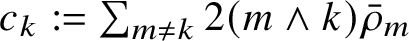 $c_k := \textstyle {\sum _{m\neq k} 2(m\wedge k)\bar {\rho }_m }$
. Because
$c_k := \textstyle {\sum _{m\neq k} 2(m\wedge k)\bar {\rho }_m }$
. Because
 $ \ell \bar {\rho }_\ell \to 0 $
, by dominated convergence we have
$ \ell \bar {\rho }_\ell \to 0 $
, by dominated convergence we have
 $ c:=\sup _k c_k = \lim _k c_k = \sum _\ell 2\ell \bar {\rho }_\ell < \frac {1}{2} $
using our assumption. Define
$ c:=\sup _k c_k = \lim _k c_k = \sum _\ell 2\ell \bar {\rho }_\ell < \frac {1}{2} $
using our assumption. Define
 $$ \begin{align*} q_{k,m} := \begin{cases} \frac{1}{c} 2(m\wedge k)\bar{\rho}_m &\text{if } m\neq k\\ \frac{1}{c} (c-c_k) &\text{if } m=k \end{cases} \qquad \text{ and } \qquad Q:=(q_{k,m})_{k,m}. \end{align*} $$
Because
 $ \sum _m 2m \bar {\rho }_m<\infty $
, we can split the sums and rewrite (1.10) as
$ \sum _m 2m \bar {\rho }_m<\infty $
, we can split the sums and rewrite (1.10) as
 $$ \begin{align} v_k &= k + c\, v_k - c\, (Qv)_k\,=\, \displaystyle{\frac{k -c\, (Qv)_k}{1-c} }, \quad v_k \in [0,\infty). \end{align} $$
Note that
 $(Qv)_k$
is finite for solutions v to (7.1).
$(Qv)_k$
is finite for solutions v to (7.1).
Let v and
 $\tilde {v}$
be two solutions to (1.10), and denote
$\tilde {v}$
be two solutions to (1.10), and denote
 $ r_k := v_k-\tilde {v}_k$
. Then
$ r_k := v_k-\tilde {v}_k$
. Then
 $$ \begin{align*} s_k := |r_k| = a \, |(Qr)_k| \leqslant a \, (Qs)_k, \end{align*} $$
where
 $a := c/(1-c) < 1$
. By induction, for all
$a := c/(1-c) < 1$
. By induction, for all
 $ n\in \mathbb {N} $
,
$ n\in \mathbb {N} $
,
 $$ \begin{align} s_k \leqslant a^n \, (Q^n s)_k. \end{align} $$
The measure
 $\pi =(\pi _k)_{k\geqslant 1}$
given by
$\pi =(\pi _k)_{k\geqslant 1}$
given by
 $$ \begin{align*}\pi_k := \frac{\bar{\rho}_k}{\sum_\ell \bar{\rho}_\ell}\end{align*} $$
satisfies
 $\pi Q=\pi $
. Because
$\pi Q=\pi $
. Because
 $ \frac {1}{1-c}<2 $
and
$ \frac {1}{1-c}<2 $
and
 $ q_{k,m}\geqslant 0 $
, solutions to (7.1) satisfy
$ q_{k,m}\geqslant 0 $
, solutions to (7.1) satisfy
 $v_k\leqslant 2k $
and
$v_k\leqslant 2k $
and
 $$ \begin{align*} \pi v = \textstyle{\sum_k v_k\, \bar{\rho}_k\, \bigl(\sum_\ell \bar{\rho}_\ell \bigr)^{-1}\, \leqslant\, 2\sum_k k\,\bar{\rho}_k\, \bigl(\sum_\ell \bar{\rho}_\ell \bigr)^{-1}} <\infty. \end{align*} $$
Likewise,
 $ \pi \tilde {v}<\infty $
and
$ \pi \tilde {v}<\infty $
and
 $ \pi s \leqslant \pi v + \pi \tilde {v} < \infty $
. Using (7.2) and
$ \pi s \leqslant \pi v + \pi \tilde {v} < \infty $
. Using (7.2) and
 $ Q $
-invariance of
$ Q $
-invariance of
 $\pi $
,
$\pi $
,
 $$ \begin{align*} \textstyle{ \pi_k s_k \leqslant \pi s \leqslant a^n \, \pi Q^n s = a^n \, \pi s, } \end{align*} $$
for every
 $ n \in \mathbb {N} $
. Hence, if
$ n \in \mathbb {N} $
. Hence, if
 $\bar {\rho }_k>0$
, then
$\bar {\rho }_k>0$
, then
 $\pi _k>0$
and
$\pi _k>0$
and
 $|r_k|=0$
, implying
$|r_k|=0$
, implying
 $v_k=\tilde {v}_k$
. When
$v_k=\tilde {v}_k$
. When
 $\bar {\rho }_k=0$
we have
$\bar {\rho }_k=0$
we have
 $v_k$
is a function of
$v_k$
is a function of
 $(v_m:\bar {\rho }_m>0)$
, implying uniqueness also in this case.
$(v_m:\bar {\rho }_m>0)$
, implying uniqueness also in this case.
Acknowledgements
We thank Roberto Fernández and Davide Gabrielli for very helpful discussions. We thank the referees for a very careful reading and suggestions that greatly improved the article.
Financial support
PAF was partially supported by Argentinian grants ANPCyT (PICT 2015-3583, 2018-02842) and UBACyT 20020160100155BA.
Conflict of Interest
None.


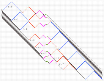


 Open access