


1. Introduction
Rational expectations have long been a cornerstone in macroeconomic modeling. Over the last five decades, a substantial body of macroeconomic and experimental economics literature has evaluated the rational expectations equilibrium (REE) hypothesis. One notable finding from the macroeconomics literature is that models with the strong form of rational expectations can lead to erratic implications, such as the forward guidance puzzle. Consequently, researchers have become increasingly skeptical of this assumption and have proposed alternative frameworks (e.g., Angeletos & Lian, Reference Angeletos and Lian2018; Farhi & Werning, Reference Farhi and Werning2019; García-Schmidt & Woodford, Reference García-Schmidt and Woodford2019).
Experimental evidence from “learning-to-forecast” experiments further calls into question the validity of the REE hypothesis. These experiments, pioneered by Marimon and Sunder (Reference Marimon and Sunder1993), reveal that participants’ behaviors often diverge from the rational expectations benchmark, especially when the aggregate outcome is determined endogenously by individual forecasts in the presence of positive expectational feedback between the aggregate outcome and individual forecasts (Bao et al., Reference Bao, Hommes and Makarewicz2017; Heemeijer et al., Reference Heemeijer, Hommes, Sonnemans and Tuinstra2009; Hommes et al., Reference Hommes, Sonnemans, Tuinstra and van de Velden2005).Footnote 1 The presence of expectational feedback—where individual expectations influence the aggregate outcome, which in turn shapes future expectations—can lead to dynamics that are better captured by models incorporating backward-looking expectation formation (Anufriev & Hommes, Reference Anufriev and Hommes2012; Evans et al., Reference Evans, Gibbs and McGough2025).Footnote 2
However, most existing learning-to-forecast experiments are essentially of the single-period type.Footnote 3 Participants only need to forecast the outcome of today or in one future period (e.g., tomorrow), and the realized outcome is a function of submitted forecasts regarding this single period (seeBao et al., Reference Bao, Hommes and Pei2021, for a survey).Footnote 4 As a result, it is difficult to provide useful insights for macroeconomists who study expectation formation in a multi-period environment and policymakers who need to know how agents form expectations to design better policies in a dynamic world. In typical macroeconomic models and dynamic games more generally, individuals forecast not only the actions of others in one period but also their actions in multiple future periods, and these forecasts about multiple future periods determine current outcomes. The single-period framework does not enable us to analyze how these series of expectations change in such a multi-period environment, such as in response to news about future shocks.
To fill this gap in the literature, we propose and conduct a novel experiment of a multi-period beauty contest game where participants submit a sequence of forecasts for multiple future periods. Based on this new experimental framework, we examine how individuals revise their expectations in response to new information, as well as how they form forecasts during normal periods without such information. We aim to contribute to the literature by providing this new dynamic experimental framework, offering a new method to assess the forward-lookingness of expectations, and identifying a new strategic environmental effect.
Our experiment is motivated by the core component of the canonical New-Keynesian model (e.g., Woodford (Reference Woodford2003) and Galí (Reference Galí2015), initially developed by Calvo (Reference Calvo1983)). In our theoretical model, there are many firms, and each firm faces the same linear demand curve. The demand for a given firm depends on its own price and the aggregate price level. While an increase in the firm’s own price reduces the demand for that firm, demand may increase or decrease when other firms raise their prices. If firms can set their prices freely, they choose prices to maximize profit, taking other firms’ prices as given. An REE price is a fixed point in this process and is often referred to as the optimal flexible price.
Following Calvo (Reference Calvo1983), we introduce a friction that limits firms’ ability to choose the optimal flexible price. Instead, firms can only change their prices with a probability of  $1-\theta.$ This constraint induces them to take future prices into account because future profit depends on current price choices; if prices cannot be adjusted later, firms must compete in future periods with the price selected today. Hence, they must incorporate future market conditions and price expectations into their current decisions. This mechanism introduces an additional dynamic expectational feedback effect, since beliefs about future prices influence today’s actions.
We transform our theoretical model into a multi-period version of the learning-to-forecast game in Marimon and Sunder (Reference Marimon and Sunder1993). In each period, participants submit forecasts for prices in multiple future periods all at once. These forecasts determine not only participants’ payoffs but also the realized aggregate prices. We set up our game so that participants merely need to anticipate aggregate prices accurately and their payoffs are maximized when they submit accurate forecasts in each period, regardless of whether the game features strategic substitutes or complements. We formally show the equivalence between this transformed experiment and the original price-setting game in Appendix A.
We adopt a three-by-two between-subjects experimental design that varies two key dimensions. The first dimension pertains to the structure of strategic interaction among participants, contrasting conditions of strong strategic complementarity with those involving equally strong or greater degrees of substitution. The second dimension concerns the timing of information about upward shifts in the demand curve, which we call shocks. In some treatments, participants face shocks that occur unexpectedly. Such shocks are referred to as unanticipated shocks. In others, they are announced two periods in advance. Such announcements of future shocks are termed anticipated shocks. This experimental design allows us to investigate both how the strategic environment affects behavior and whether participants form forward-looking expectations in response to anticipated shocks.
We begin by examining the strategic environment effect, which posits that prices deviate substantially from REE prices—that is, prices expected under REE—when the game features strategic complements, whereas prices converge quickly to REE prices otherwise. Re-examination of this well-established strategic environment effect in the literature serves as a sanity check to ensure that our experimental framework produces results that are aligned with those of existing one-period learning-to-forecast games (see, e.g.,Bao et al., Reference Bao, Hommes, Sonnemans and Tuinstra2012; Bao et al., Reference Bao, Hommes and Makarewicz2017; Bao & Hommes, Reference Bao and Hommes2019; Heemeijer et al., Reference Heemeijer, Hommes, Sonnemans and Tuinstra2009).Footnote 5 We find that the strategic environment effect is replicated in our new experimental framework, thereby validating the internal consistency of our setup before we move on to more substantive analyses.
Having reproduced the strategic environment effect in our experimental framework, we proceed to investigate the forward-looking nature of expectation formation. In particular, we examine how participants respond to anticipated shocks; namely, the announcement of future shocks. Recall that the key innovation of our design is that participants submit a sequence of forecasts extending into future periods, including those after an announced shock has occurred. For example, when a shock scheduled two periods ahead is announced in advance, we can analyze how participants revise their forecasts for periods after the realization of the shock following the announcement by comparing the forecasts for the same future periods before and after the announcement. This feature highlights the novelty of our approach; rather than relying solely on forecasts made for the immediate next period, we explicitly capture adjustments that unfold after anticipated shocks have materialized.
Our experimental data reveal significant heterogeneity in how participants respond to the anticipated shocks. While certain individuals forecast price levels that surpass those implied by the REE, others completely ignore anticipated shocks. The latter response is consistent with level-0 reasoning. This result is similar to the one based on the responses to the unanticipated shocks reported by Evans et al. (Reference Evans, Gibbs and McGough2025) in their single-period setting.
Although the heterogeneity in behavior is noteworthy in its own right, our experimental framework permits us to direct attention to the average responses of participants and to evaluate whether these are consistent with forward-looking behavior.Footnote 6 Our analysis demonstrates that, on average, participants do respond to the anticipated shocks in line with forward-looking behavior. This finding provides new evidence of forward-lookingness in expectation formation, offering a distinctive contribution to the literature.
After examining participants’ responses to anticipated shocks, we turn to the formation of expectations during periods that lack such shocks. That is, we focus on “normal” times to study belief formation in a dynamic environment. Following Anufriev and Hommes (Reference Anufriev and Hommes2012), we estimate a reduced-form forecasting rule that encompasses various heuristics like adaptive expectations and trend following. We generalize their approach by allowing coefficients of these heuristics to vary across different forecast horizons.
The regression results show that most participants rely heavily on the most recent price as a reference point, with coefficients close to one, and they also consider their past forecast errors, indicating self-referential expectations. Notably, the impact of recent price changes becomes stronger as the forecast horizon lengthens. This effect is particularly strong in positive feedback environments, where participants increasingly rely on trend-following behavior. This finding suggests that in positive feedback environments (i.e., those with strategic complementarity), participants expect price increases to persist, potentially leading to de-anchored long-run inflation expectations. Conversely, in negative feedback settings (i.e., those with strategic substitutability), participants view price increases as temporary, and their expectations remain relatively stable across horizons.
Taken together, these findings indicate an important policy implication: expectation formation depends qualitatively on whether the strategic environment features complementarity or substitutability. As a result, central banks must understand the strategic context in which agents operates to effectively conduct monetary policy and mitigate the risks of expectation de-anchoring.
The rest of the paper is organized as follows. Section 2 presents a model of a multi-period beauty contest based on Calvo (Reference Calvo1983). The experiment’s design and procedure are presented in Section 3, while Section 4 shows the REE as the benchmark. The results of the experiment are summarized in Section 5, including a discussion of implications for modeling expectation formation. Section 6 concludes.
2. A model of a multi-period beauty contest
We introduce our theoretical model and derive the equilibrium price under the REE of the model. The theoretical model serves as the foundation for our experiment design, and the REE price offers a benchmark for comparison in the subsequent analysis.
Consider a continuum of monopolistically competitive firms uniformly distributed over the interval  $\left[0,1\right]$. Each firm $i$ selects a price $p_{i}$; for simplicity, we omit the subscript $i$. The demand function for an individual firm is
 \begin{equation}
D\left(p;P\right)\equiv\left[a-bp+cP\right]^{+},
\end{equation}
\begin{equation}
D\left(p;P\right)\equiv\left[a-bp+cP\right]^{+},
\end{equation}where  $P$ represents the aggregate price given by
 \begin{equation}
P=\int_{0}^{1}p_{i}di.
\end{equation}
\begin{equation}
P=\int_{0}^{1}p_{i}di.
\end{equation} We assume that  $a \gt 0$, $b \gt 0$, and $c\in\mathbb{R}$, with the condition
 \begin{equation*}
-\infty \lt c\leq2b,
\end{equation*}
\begin{equation*}
-\infty \lt c\leq2b,
\end{equation*}which ensures the existence of an REE price in the single-period version of the game. The parameter  $c$ can be positive or negative, which governs the degree of strategic interaction among firms. All firms share an identical linear technology function with a unit production cost denoted by $\kappa.$
Each firm maximizes the present value of its profit but faces pricing frictions; firms cannot adjust their prices every period and can only do so with probability  $1 - \theta$. If a firm cannot change its price for $T$ consecutive periods, it is allowed to adjust its price with certainty in the next period.Footnote 7 Additionally, with probability $\gamma \in [0,1)$, all firms may be forced to exit the market. This assumption enables us to conduct experiments within a finite period that effectively replicate those of an infinite period (Duffy, Reference Duffy, Kagel and Roth2017).
Firms that can reset their prices in period  $t$ solve the following optimization problem:
 \begin{equation}
\max_{p_{t}} \sum_{s=0}^{T-1}((1-\gamma)\theta)^{s}\left(p_{t}-\kappa \right)D\left(p_{t};P_{t+s}\right).
\end{equation}
\begin{equation}
\max_{p_{t}} \sum_{s=0}^{T-1}((1-\gamma)\theta)^{s}\left(p_{t}-\kappa \right)D\left(p_{t};P_{t+s}\right).
\end{equation} Recall that in every period, firm  $i$ can re-optimize its price with probability $1-\theta$. Since the continuation payoffs in these future events are not a function of $p_{t},$ they do not appear in objective function (3).
We now formally define an REE as a pair of prices  $(p_t,P_t)$ such that given the aggregate price $(P_t)_t$, $p_t$ solves the maximization problem (Eq. 3), and consistency, $P_t = p_t$, holds for all $t.$
$t.$
We establish the following proposition:
Proposition 1. The optimal price for firms that can reset their prices at period  $t$ is given by
 \begin{equation}
p_{t}=\sum_{s=0}^{T-1}\frac{((1-\gamma)\theta)^{s}}{\sum_{k=0}^{T-1}((1-\gamma)\theta)^{k}}\left(\alpha+\beta P_{t+s}\right),
\end{equation}
\begin{equation}
p_{t}=\sum_{s=0}^{T-1}\frac{((1-\gamma)\theta)^{s}}{\sum_{k=0}^{T-1}((1-\gamma)\theta)^{k}}\left(\alpha+\beta P_{t+s}\right),
\end{equation}where
 \begin{equation*}
\alpha=\frac{1}{2}\left(\kappa+\frac{a}{b}\right)\quad\beta=\frac{1}{2}\frac{c}{b}.
\end{equation*}
\begin{equation*}
\alpha=\frac{1}{2}\left(\kappa+\frac{a}{b}\right)\quad\beta=\frac{1}{2}\frac{c}{b}.
\end{equation*}Moreover, the aggregate REE price evolves according to
 \begin{equation}
P_{t} =\left(1-\theta\right)p_{t}+\theta P_{t-1}.
\end{equation}
\begin{equation}
P_{t} =\left(1-\theta\right)p_{t}+\theta P_{t-1}.
\end{equation}Proof. Taking the first-order conditions of the maximization problem in Eq. (3), we obtain Eq. (4). To derive Eq. (5), recall that the aggregate price in Eq. (2) is given by the average of individual prices and that only the fraction  $1-\theta$ of firms can reset their prices. Because firms that cannot reset their prices today are randomly chosen, the average price among them is $P_{t-1}$. Firms that can reset their prices choose the same price level given by Eq. (4), so the average price $P_t$ satisfies Eq. (5).
Notably,  $\alpha+\beta P_{t}$ represents the optimal price in period $t$ if firms can reset their prices freely. This price is often referred to as the optimal flexible price. Therefore, the optimal price in our environment, as shown in Eq. (4), constitutes a weighted average of optimal flexible prices. Eq. (4) captures the dynamic thought process within firms; the optimal price, $p_{t}$, depends on current actions by others, and on future actions, represented by $\left(P_{t+s}\right)_{s=0}^{T-1}$. Because of this inter-period interdependence, today’s aggregate price is also influenced by expectations of future prices. This feature leads to the model being referred to as a dynamic beauty contest model (e.g.,
Angeletos & Lian, Reference Angeletos and Lian2018).
$\left(P_{t+s}\right)_{s=0}^{T-1}$. Because of this inter-period interdependence, today’s aggregate price is also influenced by expectations of future prices. This feature leads to the model being referred to as a dynamic beauty contest model (e.g.,
Angeletos & Lian, Reference Angeletos and Lian2018).
By contrast, when firms can adjust prices without friction,  $\theta = 0$, the dynamic aspect disappears, and firms focus solely on predicting other firms’ current actions. Our proposed experiment, inspired by this model, differs from existing single-period experiments by explicitly requiring participants to anticipate not only others’ actions in period $t$ but also in subsequent periods $t+1, \ldots, t+T-1$.
3. Experimental design
In this section, we describe the experimental setup by detailing the structure of the learning-to-forecast game that participants actually play. We then outline our treatment design, followed by an explanation of the online experimental procedure.
3.1. Setup
In our experimental setup, we employ groups of six participants.Footnote 8 These participants, indexed by  $i$, engage in the game over multiple periods. At the beginning of each period, they submit their price forecasts for the next five periods including the current one; that is, $T=5$.Footnote 9 For example, in the first period, participants submit their price forecasts for periods 1 to 5. In the second period, they provide forecasts for periods 2 to 6, and so on. We denote the forecast of the price in period $k$ submitted in period $t$ as $f_{t,k}^{i}$. While not all submitted forecasts impact participants’ rewards, as detailed below, all five forecasts have the potential to do so when submitted.Footnote 10
Let  $\pi_{t}^{i}$ denote the reward of participant $i$ in period $t$, as determined by
 \begin{equation*}
\pi_{t}^{i}=\frac{100}{\left|F_{t}^{i}-P_{t}\right|+1},
\end{equation*}
\begin{equation*}
\pi_{t}^{i}=\frac{100}{\left|F_{t}^{i}-P_{t}\right|+1},
\end{equation*}where  $P_{t}$ is the realized price in period $t$, and $F_{t}^{i}$ is the payoff-relevant forecast of participant $i$ in period $t$, as defined below.Footnote 11 If the reward is not an integer, then it is rounded to the nearest integer.
In the first period  $t$, the payoff-relevant forecast $F_{t}^{i}$ is set to $F_{1}^{i}=f_{1,1}^{i}.$ In period $2$, the payoff-relevant forecast $F_2^i$ is determined probabilistically: with probability $1-\theta,$ the newly submitted set of forecasts become payoff-relevant, yielding $F_{2}^{i}=f_{2,2}^{i};$ with probability $\theta,$ the previous forecasts remain payoff-relevant, resulting in $F_{2}^{i}=f_{1,2}^{i}$. This process continues in subsequent periods. If the same set of forecasts has been payoff-relevant for five consecutive periods (i.e., a firm cannot reset its price for five consecutive periods), then the new set of forecasts submitted in the next period becomes payoff-relevant with certainty.
This adjustment process is motivated by the multi-period beauty contest model introduced in Section 2. The probability of firms being given an opportunity to re-optimize their prices in period  $t$,
$t$,  $1-\theta$, is translated into the probability of the new set of forecasts becoming payoff-relevant for participants. The horizon, $T$, over which firms optimize in the model is equivalent to the number of future periods in addition to the current one over which our participants forecast in each period. As in Marimon and Sunder (Reference Marimon and Sunder1993) and Bao et al. (Reference Bao, Hommes and Makarewicz2017), we set the payoffs so that the equilibrium path of the Nash equilibrium (subgame perfect Nash equilibrium) corresponds to the REE of the multi-period beauty contest game in Section 2. See Appendix A for a formal proof.
To illustrate how submitted forecasts determine the payoff-relevant forecasts, consider the hypothetical forecasts of participant  $i$ shown in Table 1. Each row lists the forecasts submitted in period $t$. For example, in period $t=1,$ the participant submits forecasts of the prices for periods $1$ to $5$:
$5$:
 \begin{equation*}
\left(f_{1,1}^{i},f_{1,2}^{i},f_{1,3}^{i},f_{1,4}^{i},f_{1,5}^{i}\right)=\left(10,11,12,12,12\right).
\end{equation*}
\begin{equation*}
\left(f_{1,1}^{i},f_{1,2}^{i},f_{1,3}^{i},f_{1,4}^{i},f_{1,5}^{i}\right)=\left(10,11,12,12,12\right).
\end{equation*}Hypothetical submitted forecasts

In period 1, this set of forecasts becomes payoff-relevant so that the payoff-relevant forecast is  $F_{1}^i=10$. In period $2,$ the participant submits new forecasts $f^i_{2,2},\cdots, f^i_{2,6}$. Suppose that the new forecasts do not become payoff-relevant in period 2. Then, $F_2^i = f_{1,2}^i =11$. If the new set of forecasts becomes payoff-relevant in periods 3 and 4, then the latest forecasts determine the payoff-relevant forecasts. Thus, $F_{3}^{i}= f_{3,3}^i= 9$ and $F_{4}^{i} = f_{4,4}^i = 13$.Footnote 12 The reward for the participant is determined by the difference between the payoff-relevant forecasts $F_t^i$ and the aggregate price $P_t$.
We now explain how the aggregate price is determined in our experiments; all participants submit their forecasts simultaneously every period, and these submitted forecasts jointly determine the aggregate price  $P_{t}$. Based on the model in Section 2, the aggregate price is given by
 \begin{equation}
P_{t}=\frac{1}{6}\left(\sum_{i\,\text{cannot reset}} p^i_{t-1} + \sum_{i\,\text{can reset}}\sum_{j=0}^{T-1}\frac{((1-\gamma) \theta)^{j}}{\sum_{l=0}^{T-1}((1-\gamma) \theta)^{l}}\left(\alpha+\beta f_{t,t+j}^{i}\right) \right),
\end{equation}
\begin{equation}
P_{t}=\frac{1}{6}\left(\sum_{i\,\text{cannot reset}} p^i_{t-1} + \sum_{i\,\text{can reset}}\sum_{j=0}^{T-1}\frac{((1-\gamma) \theta)^{j}}{\sum_{l=0}^{T-1}((1-\gamma) \theta)^{l}}\left(\alpha+\beta f_{t,t+j}^{i}\right) \right),
\end{equation}where  $\alpha$ and $\beta$ are parameters of the model and specified later. Eq. (6) is the empirical-counterpart of Eq. (2). The first term on the right-hand side of Eq. (6) represents the prices of participants who are unable to adjust their prices. The second term corresponds to the prices of participants who can reset their prices. The mapping of submitted forecasts to the optimal price is given by Eq. (4).
On the screen in which participants submit their forecasts, the values of  $\alpha$ and $\beta$ are presented clearly. On the same screen, participants are informed of the realized $P_t$ and the payoff-relevant forecast $F_t$ in all past periods. See Appendix G for the screenshots.
In our experiment, we set the reset probability  $\theta$ to $1/2$ and assume that the game ends with probability $\gamma=0.05$ at the end of each period.Footnote 13 Participants are rewarded based on the total points they earn throughout the game. As noted above, we set $T=5.$ Eq. (6) can be used to provide a justification for $T=5.$ Note that when $\theta = 1/2$ and $\gamma=0.05$, the impact of $f^i_{t,t+4}$ on the optimal price is minimal. This is because the weight of $f^i_{t,t+4}$ is $((1-\gamma)\theta)^4/\sum_{k=0}^4((1-\gamma)\theta)^k$, which is approximately 0.027. Therefore, allowing participants to make longer forecasts is unlikely to change the results.
While it is conceptually trivial to end a game stochastically, implementing such a probabilistic termination rule in a laboratory experiment poses challenges, either because the game might end too soon to study the evolution of the forecasts in response to shocks, or the game might not end within the scheduled time for participants. To address these challenges, we use the block random termination method (Fréchette & Yuksel, Reference Fréchette and Yuksel2017) commonly used in experiments involving indefinitely repeated games.
Under this method, participants play the game in blocks of  $B$ periods. During each block, the game proceeds without participants knowing whether or not it has ended. Only at the end of a block are participants informed if the game actually ended at some point during that block.Footnote 14 If the game has ended during the block, they receive the sum of their payoffs $\pi_{t}^{i}$ up to the period when the game ended. For example, if the game actually ended in period $\tau$ where $\tau \lt B$, participants are rewarded based on $\sum_{t=1}^{\tau}\pi_{t}^{i}$. If the game has not ended, it continues into the next block of $B$ periods. They are also informed that the game can continue beyond $B$ periods; if that happens, they play the game for at least another $B$ periods. In our experiment, we set $B = 20$, so participants are told they will play the game for at least 20 periods.
To minimize variation in experiment duration and participant payments across sessions, we followed the procedure of Duffy and Puzzello (Reference Duffy and Puzzello2014); Duffy and Puzzello (Reference Duffy and Puzzello2022) by predefining the random number sequence. Predefining ensured that all sessions repeated two blocks and concluded after the first game. Consistent with Duffy and Puzzello (Reference Duffy and Puzzello2014); Duffy and Puzzello (Reference Duffy and Puzzello2022), this information was not disclosed to participants.Footnote 15
During the games, we introduce (a maximum of) two shocks to  $\alpha$, which affects the demand size, during the first two blocks of 20 periods (one shock in each block). The literature suggests that under strategic substitution, where prices often converge to the steady state level, it may take several periods to do so. To allow for the prices to stabilize before introducing a shock, we introduced the first shock at the beginning of period 14 and the second at period 29. We assume that the initial flexible REE price is 65; it becomes 85 and 110 after the first and the second shocks, respectively. We choose $\alpha$ to match these price levels for each value of $\beta.$
3.2. Treatments
Our three-by-two between-participants experiment focuses on varying two main aspects of the games. The first is the degree of strategic interaction. We consider games where  $\beta$ takes values in $\left\{0.9,-0.9,-1.8\right\}$; that is, the games exhibit either strategic complementarity (positive feedback) or substitution (negative feedback).Footnote 16 We also explicitly consider a case of strong substitution with $\beta=-1.8$. This consideration is motivated by the fact that although New Keynesian models may exhibit strong substitutability, as demonstrated by García-Schmidt and Woodford (Reference García-Schmidt and Woodford2019), the issue has not been investigated to a greater extent in the experimental literature, with exceptions such as Bao and Duffy (Reference Bao and Duffy2016) and Evans et al. (Reference Evans, Gibbs and McGough2025).
The second is the announcement of the shocks to  $\alpha$. We examine treatments both with and without pre-announcement of shocks. In the treatment without pre-announcement, participants are informed of the new value of $\alpha$ only when the shocks occur—that is, in period 14 for the first shock and in period 29 for the second shock. In the treatments with pre-announcement, participants are informed of the new value of $\alpha$ two periods before its realization, that is, in period 12 for the first shock and in period 27 for the second shock. This announcement specification is desirable because announcing the shocks two periods in advance allows us to examine participants’ forecasts for prices after the realization of shocks, both before and after the announcements.Footnote 17 Because we elicit participants’ forecasts only for five future periods, if the announcement is made either too early in advance, it becomes impossible to analyze its immediate impact on forecast revisions at the time the shock occurs. Therefore, we make the announcement two periods prior to the occurrence of the shock and analyze how forecasts are revised, the question that lies at the core of our study.
3.3. Procedures
Our experiments were conducted online using oTree (Chen et al., Reference Chen, Schonger and Wicken2016), an open source platform for web-based interactive tasks. Participants joined from their own locations instead of our physical laboratory. We used Zoom to manage and coordinate the experiments.Footnote 18
Once participants had received general instructions about the online experiment and were prepared, the prerecorded instruction video was shown on their screen. Although they did not receive physical copies of the instruction slides, participants were informed that they could access the same slides after the video finished, and until they finished the comprehension quiz. To begin the first game, all participants had to correctly answer all six quiz questions.Footnote 19 Final rewards were provided through Amazon Gift Cards (e-mail version).
We recruited participants, who were students at the University of Osaka, using ORSEE (Greiner, Reference Greiner2015). An English translation of the instruction slides, examples of the decision screens, and the comprehension quiz are provided in Appendix F.
4. Benchmark analysis: rational expectations equilibrium
We take rational expectations as our benchmark. As shown in Proposition 1, the REE aggregate price denoted by  $\left(P^{REE}_{t}\right)$ is characterized by Eqs. (4) and (5) given the initial condition, $P_{-1}$. Unlike in the theoretical analysis, parameter $\alpha$ is time-varying in our experiment. Thus, we need to generalize Proposition 1 to accommodate this case. It is straightforward to show that the REE price with time-varying $\alpha$ satisfies the following equation:
 \begin{equation}
P^{REE}_{t} =\left(1-\theta\right)\sum_{k=t}^{T-t-1}\frac{((1-\gamma)\theta)^{k-t}}{\sum_{s=0}^{T}((1-\gamma)\theta)^{s}}\left(\alpha_{t,k}+\beta P^{REE}_{t+k}\right)+\theta P^{REE}_{t-1},
\end{equation}
\begin{equation}
P^{REE}_{t} =\left(1-\theta\right)\sum_{k=t}^{T-t-1}\frac{((1-\gamma)\theta)^{k-t}}{\sum_{s=0}^{T}((1-\gamma)\theta)^{s}}\left(\alpha_{t,k}+\beta P^{REE}_{t+k}\right)+\theta P^{REE}_{t-1},
\end{equation}where  $\alpha_{t,k}$ is the expected value of $\alpha$ in period $k$ from the period- $t$ perspective. When the shocks are not announced in advance, $\alpha_{t,k}=\alpha_{t,t}$ for all $k$ and $t.$ When the shocks occur, $\alpha_{t,t}$ suddenly increases. Suppose that the shocks are pre-announced. In that case, $\alpha_{t,k}$ changes when the shocks are announced, not when they occur. Again, the pre-announcement of the future shocks, anticipated shocks, matters only if the game is a multi-period beauty contest game. If firms do not face any pricing frictions $\theta=0$, then the anticipated shocks have no effect on the REE price.
Figure 1 shows the REE price sequence  $\left(P^{REE}_{t}\right)_{t}$ when the shocks are announced two periods in advance (left panel) and when they are not announced (right panel). These figures can be intuitively understood. When the game demonstrates strategic complementarity ( $\beta \gt 0$), the transition to new steady state equilibrium prices is slower due to Calvo pricing friction. Participants recognize that others may not adjust their prices swiftly because of that pricing friction. Since individual optimal prices are positively related to others’ pricing decisions, participants prefer to adjust their prices slowly.
Aggregate price  $P_{t}$ under rational expectation

By contrast, when the game exhibits strategic substitution ( $\beta \lt 0$), the mechanism operates in the opposite direction. If some agents fail to adjust their prices, the prevailing price becomes excessively low. This low price incentivizes agents to increase their prices. Consequently, the transition to the new steady state equilibrium price occurs more rapidly.
5. Analysis of the experimental data
In this section, we begin by outlining the experimental sessions, including participant numbers, treatment assignments, and earnings. Then, we proceed to analyze our experimental data.
5.1. Overview of the experimental sessions
We conducted our experiments in April and May 2023, involving a total of 294 participants.Footnote 20 Table 2 summarizes the number of groups per treatment. Each experiment lasted for approximately 90 minutes, and participants earned 2482 JPY (approximately 18 USD based on the exchange rate at the time), including a show-up fee of 500 JPY on average.Footnote 21 The average payment varied across the value of  $\beta$. It was lowest in the treatments with $\beta=-1.8$ (1778 JPY), followed by 2806 JPY and 2844 JPY in treatments with $\beta=-0.9$ and $\beta=0.9$, respectively.
Number of groups per treatment

Notes: “With Announcement” represents the results where the shocks were announced, while “Without Announcement” shows the results where the shocks were not pre-announced.  $a$: One group stopped at $t=33$ due to a technical problem. $b$: One group stopped at $t=39$ due to a technical problem.
5.2. Aggregate price dynamics
We begin by presenting the dynamics of prices observed in each treatment in Figure 2. Each line represents a group within each panel. As observed, irrespective of whether an announcement is made, the prices follow the REE price closely when the game exhibits strategic substitutes  $\beta \lt 0.$ When the game exhibits strategic complements $\beta \gt 0$, they deviate persistently from the REE prices. As shown by Fehr and Tyran (Reference Fehr and Tyran2008), these features can be understood intuitively. When the game exhibits strategic complements, the best response function has a positive slope, and participants have a strong motive to choose a similar price level of others. Consequently, the realized price remains close to the initial expectation of others’ actions, and the initial expectation fulfills itself. This self-fulfilling mechanism makes the adjustment slow, leading to persistent deviations from the REE price. When the game exhibits strategic substitutes, this mechanism does not operate. Participants want to choose higher (lower) prices when others choose lower (higher) prices. Thus, their initial expectations are not self-fulfilling unless they coincide with the REE price, and they often quickly converge toward the REE price. Note that our experimental findings are also found in existing learning-to-forecast experiments, such as those by Heemeijer et al. (Reference Heemeijer, Hommes, Sonnemans and Tuinstra2009), Bao et al. (Reference Bao, Hommes, Sonnemans and Tuinstra2012); Bao et al. (Reference Bao, Hommes and Makarewicz2017), and Bao and Hommes (Reference Bao and Hommes2019).
Realized aggregate prices  $P_{t}$ (a) Positive Feedback: $\beta=0.9$ (b) Weak Negative Feedback: $\beta=-0.9$ (c) Strong Negative Feedback: $\beta=-1.8$

It is evident that aggregate prices become more stable when the game has weak strategic substitutes ( $\beta = -0.9$). By contrast, with strong strategic substitutes ( $\beta = -1.8$), aggregate prices hover around the REE price but exhibit greater deviations. A similar pattern is also documented by Bao and Duffy (Reference Bao and Duffy2016) and Evans et al. (Reference Evans, Gibbs and McGough2025). This result likely stems from difficulties in expectation coordination. When $\beta$ becomes more negative, the price depends sensitively on expectations. This sensitivity results in the observed instability of prices.Footnote 22
5.3. Effect of the degree of strategic interaction
We proceed to quantify the degree of deviation from the REE prices by following the methodology developed by Stöckl et al. (Reference Stöckl, Huber and Kirchler2010), which allows us to verify that our results align with evidence from existing one-period learning-to-forecast games. We compute the relative absolute deviation (RAD) and the relative deviation (RD) as proposed in their study. For each group  $g$,
$g$,  $RAD_{g}$ and $RD_{g}$ are calculated as follows:
 \begin{align*}
RAD_{g} & =\frac{1}{K}\sum_{t}\frac{\left|P_{g,t}-P_{t}^{REE}\right|}{P_{t}^{REE}}\\
RD_{g} & =\frac{1}{K}\sum_{t}\frac{P_{g,t}-P_{t}^{REE}}{P_{t}^{REE}},
\end{align*}
\begin{align*}
RAD_{g} & =\frac{1}{K}\sum_{t}\frac{\left|P_{g,t}-P_{t}^{REE}\right|}{P_{t}^{REE}}\\
RD_{g} & =\frac{1}{K}\sum_{t}\frac{P_{g,t}-P_{t}^{REE}}{P_{t}^{REE}},
\end{align*}where  $P_{g,t}$ is the realized period $t$ price for group $g$,
$g$,  $P_{t}^{\text{REE}}$ is the REE price in period $t$, and $K$ represents the total number of periods (40 except for the two groups that faced a technical problem).Footnote 23
Figure 3 shows the empirical cumulative distributions of RADs (top) and RDs (bottom) in the treatments with (left) and without (right) an announcement. In each panel, the distributions for each  $\beta$ are shown. The top panels show that regardless of the existence of an announcement, RADs are positive for each $\beta$. Applying the signed-rank test to the distributions of RADs, the observed prices are significantly different from the REE prices.Footnote 24 Furthermore, the distributions of RADs are ranked in terms of first-order stochastic dominance; regardless of whether an announcement was made, the distribution under $\beta = 0.9$ stochastically dominates those under $\beta = -1.8$ and $\beta = -0.9$. This indicates a higher likelihood of larger deviations from the REE prices under $\beta = 0.9$ than with other treatments, and the differences between the three treatments are statistically significant both with and without an announcement.Footnote 25 The deviations from the REE prices are smallest under weak substitution ( $\beta = -0.9$), larger under strong substitution ( $\beta = -1.8$), and largest under strategic complementarity ( $\beta = 0.9$).
Deviations from the rational expectation prices (a) Relative Absolute Deviation (RAD) (b) Relative Deviation (RD)

The bottom panels in Figure 3 build on these findings by showing that RDs are also larger under strategic complementarity than under strategic substitution, mirroring the pattern observed for RADs. However, in contrast to the results for RADs, there is no longer a statistically significant difference between  $\beta = -0.9$ and $\beta = -1.8$.Footnote 26 The lack of statistical significance comes from the fact that RDs, by incorporating the direction of deviation from the REE price, become nearly zero when prices fluctuate around the REE price, as in the case where $\beta = -1.8$.Footnote 27
5.4. Forward-lookingness of expectations
We now examine whether forecasts have responded to anticipated shocks: that is, the announcement of future shocks.Footnote 28 To accomplish this objective, we analyze forecast revisions before and after anticipated shocks to assess whether individuals have reacted to the shocks or disregarded them. In particular, if there are no revisions to forecasts after an anticipated shock, it suggests that the anticipated shock is ignored.Footnote 29
To operationalize this analysis, we define our measures of forecast revisions as follows. We focus on the forecasts for changes in prices during periods 14 and 29,  $P_{14}-P_{13}$ and $P_{29}-P_{28}$, and analyze how these forecasts are revised before and after the associated shock announcements. These revisions are mathematically represented as
 \begin{equation}
\Delta f^i_{1} = E^i\left[P_{14}-P_{13}\mid t\leq13\right]-E^i\left[P_{14}-P_{13}\mid t\leq11\right], \mbox{and }
\end{equation}
\begin{equation}
\Delta f^i_{1} = E^i\left[P_{14}-P_{13}\mid t\leq13\right]-E^i\left[P_{14}-P_{13}\mid t\leq11\right], \mbox{and }
\end{equation} \begin{equation}
\Delta f^i_{2} = E^i\left[P_{29}-P_{28}\mid t\leq28\right]-E^i\left[P_{29}-P_{28}\mid t\leq26\right],
\end{equation}
\begin{equation}
\Delta f^i_{2} = E^i\left[P_{29}-P_{28}\mid t\leq28\right]-E^i\left[P_{29}-P_{28}\mid t\leq26\right],
\end{equation} where the conditional expectations are taken over the relevant information sets. For example,  $E^i\left[P_{14}-P_{13}\mid t\leq13\right]$ represents the expected value of the change of the price in period 14 conditional on all information available up to period 13. Thus, the differences in the conditional expectations, $\Delta f^i_{1}$ and $\Delta f^i_{2}$, capture the revisions of the forecasts of price changes $P_{14}-P_{13}$ and $P_{29}-P_{28}$ in response to the announcements in period 12 and 27, respectively.Footnote 30 The conditional mean is calculated based on information available through periods 13 and 28 instead of periods 12 and 27, to mitigate noise by including two post-announcement observations.
By examining whether the values of these revisions are zero or not, we can infer that individuals are responding to the anticipated shocks. In particular, observing nonzero revisions strongly suggests that participants do indeed react to the announcements. At the same time, because our analysis focuses on revisions tied to price changes, there is another way to interpret nonzero revisions: announcements exert a greater influence on forecasts for more distant future prices relative to the near term.Footnote 31 However, it is important to emphasize that identifying the forward-lookingness through these revisions is a sufficient but not strictly necessary condition. For example, even if participant  $i$ revises her forecasts of both $P_{14}$ and $P_{13}$ by 10 points each in response to the first announcement, $\Delta f_1^i$ remains at zero. Thus, according to our measure, this implies that she does not respond to the announcement. This example highlights that our inference based on the revisions provides a conservative gauge of forward-lookingness. We intentionally adopt this conservative criterion to reduce the likelihood of falsely concluding that participants are forward looking when they are not, thereby ensuring a more robust measure of genuine forward-looking behavior.
To calculate these revisions for each participant  $i$, we take advantage of our experimental design. We measure the forecasts for the price change in period 14, conditional on the information available by period 13, as $\sum_{t=12}^{13}\left(f_{t,14}^{i}-f_{t,13}^{i}\right)/2$. Recall that $f_{t,14}^{i}-f_{t,13}^{i}$ represents the forecast of $P_{14}-P_{13}$ in period $t$. Hence, this average corresponds to the conditional expectation after the first shock announcement, if any. Similarly, we measure the conditional expectation before the first shock announcement, if any, as $\sum_{t=10}^{11}\left(f_{t,14}^{i}-f_{t,13}^{i}\right)/2$. The difference of these averages corresponds to $\Delta f^i_1$. We define $\Delta f^i_2$ in an analogous way. Note that our multi-period experimental design uniquely allows us to measure these revisions. In the majority of existing papers, these revision measures are simply unavailable since sequences of forecasts are not collected.
To analyze the distributions of  $ \Delta f_{1}^{i} $ and $ \Delta f_{2}^{i} $, it is useful to compare them with their theoretical values under the REE. When the shocks are not announced, their theoretical values are easily obtained. Under the REE hypothesis, the entire path of the prices $ P_t $ is rationally expected at the beginning of the game. Thus, no additional information becomes available over time, and forecasts are not revised at all, and both $ \Delta f^i_{1} $ and $ \Delta f^i_{2} $ are zero in this case.
Consider the case where shocks are announced. Since those announcements constitute new information, they trigger revisions of the forecasts. To compute  $ \Delta f^i_{1} $ under the REE, we solve our model in Section 2 in two cases. We solve the model without any shocks and then solve it again under the assumption that the first shock is announced. We then compute the difference, $ P_{14} - P_{13} $, for both cases. Finally, we subtract the difference with no shocks from the difference with the first shock announcement. This double difference corresponds to the theoretical counterpart of $ \Delta f^i_1 $. We compute the theoretical value of $ \Delta f^i_2 $, using the same procedure.
We begin our analysis by considering the scenario where shocks are not announced. This analysis serves as a sanity check for our experimental setup since we naturally expect participants not to revise their forecasts in the absence of new information. Figure 4 presents the histograms for  $\Delta f_{1}^{i}$ and $\Delta f_{2}^{i}$ for various $\beta$ values. The figure indicates that both $\Delta f_{1}^{i}$ and $\Delta f_{2}^{i}$ for all $\beta$ are centered around zero, with their median values exactly equal to zero. To be specific, the fractions of individuals who do not revise their forecasts are greater than $40\%$. As discussed above, this result aligns with the model’s prediction under the REE; most participants do not revise their forecasts unless new information arrives. It is important to note that while our finding constitutes a necessary condition for participants to hold rational expectations, it does not suffice on its own. For example, if participants strongly believe that the environment is stationary and would assume that $P_t = P_{t+1}=\cdots$, that leads to $E^i(P_{t+1}-P_{t}|P_{\tau \lt t})=0$. In such cases, even though participants do not form their expectations based on rational expectations, $\Delta f_{1}^{i}$ and $\Delta f_{2}^{i}$ still equal zero. We examine how each participant forms her belief over the price levels in Section 5.5.
Forward-lookingness of expectations: case without announcement (a) Distributions of Forecast Revisions After the First Announcement  $\Delta f_{1}^{i}$ (b) Distributions of Forecast Revisions After the Second Announcement $\Delta f_{2}^{i}$

Next, we analyze the case where shocks are announced, as depicted in the histograms in Figure 5. Three important observations emerge from this analysis. First, the histograms appear right-skewed, and the median values have become positive, indicating that some participants respond significantly to the announcements.
Forward-lookingness of expectations: case with announcement (a) Distributions of Forecast Revisions After the First Announcement  $\Delta f_{1}^{i}$ (b) Distributions of Forecast Revisions After the Second Announcement $\Delta f_{2}^{i}$

Second, there is considerable heterogeneity in participants’ responses. To examine this heterogeneity, we compute for each treatment the fraction of participants who did not revise their forecasts ( $\Delta f_{j}^{i} = 0$), those who revised their forecasts to a greater extent than predicted by the REE model, and others. As shown in Figure 5, about a quarter of participants did not revise their forecasts, implying that they ignored the announcement when forecasting price change. However, a significant fraction of participants adjust their forecasts upward, accounting for the announcements. Notably, some even overreact by revising their forecasts more than the REE model predicts. For example, after the announcement of the second shock, $33\%$ of participants overreacted when $\beta = -0.9$. This finding suggests strong forward-looking behavior.Footnote 32
Another way to classify revisions,  $\Delta f_{j}^{i}$, is to apply level- $k$ reasoning (Nagel, Reference Nagel1995). The level- $k$ reasoning represents a form of forward-looking expectation formation and is often employed to analyze situations in which agents must make forecasts after unprecedented shocks (Farhi & Werning, Reference Farhi and Werning2019). Following Evans et al. (Reference Evans, Gibbs and McGough2025), we derive the theoretical counterparts of $\Delta f_{j}^{i}$ under level- $k$ forecasting.Footnote 33 Let the default forecast sequence be ${P_{t+s}(0)}_{s=0}^\infty$. The level- $k$ forecast sequence ${P_{t+s}(k)}_{s=0}^\infty$ is then defined recursively by
 \begin{equation}
P_{t}(k) = (1-\theta)\sum_{s=0}^{T-1}\frac{\bigl((1-\gamma)\theta\bigr)^{s}}{\sum_{m=0}^{T-1}\bigl((1-\gamma)\theta\bigr)^{m}}\bigl(\alpha+\beta P_{t+s}(k-1)\bigr)
+\theta P_{t-1}(k-1).
\end{equation}
\begin{equation}
P_{t}(k) = (1-\theta)\sum_{s=0}^{T-1}\frac{\bigl((1-\gamma)\theta\bigr)^{s}}{\sum_{m=0}^{T-1}\bigl((1-\gamma)\theta\bigr)^{m}}\bigl(\alpha+\beta P_{t+s}(k-1)\bigr)
+\theta P_{t-1}(k-1).
\end{equation} We define the default forecast sequence  $P_{t+s}(0)$ as the average of the realized prices in the two periods immediately preceding the forecast date. For example, when computing the level- $k$ theoretical forecast
 \begin{equation*}
E^i\bigl[P_{14}-P_{13}\mid t\leq13\bigr],
\end{equation*}
\begin{equation*}
E^i\bigl[P_{14}-P_{13}\mid t\leq13\bigr],
\end{equation*}we set
 \begin{equation*}
P_{t+s}(0)=\frac{P_{12}+P_{13}}{2}
\quad\text{for all }s\ge0.
\end{equation*}
\begin{equation*}
P_{t+s}(0)=\frac{P_{12}+P_{13}}{2}
\quad\text{for all }s\ge0.
\end{equation*}We then assign each participant to the level whose theoretical forecast lies closest to her observed revision. Participants whose revisions deviate by more than three units from all level-0, level-1, level-2, and REE forecasts are categorized as “Others.” The cutoff of three follows Evans et al. (Reference Evans, Gibbs and McGough2025). Figure 6 shows the results.
Classification of participants based on depth of reasoning

As expected from Figure 5, large shares of participants are classified as level-0 forecasters since they do not revise their forecasts at all. Moreover, sizable shares fall into each of the level-0 through level-3 and REE categories even in our setting. These results mirror those reported by Evans et al. (Reference Evans, Gibbs and McGough2025). One notable quantitative divergence is that the share of participants whose forecasts conform to the REE benchmark is smaller here than in Evans et al. (Reference Evans, Gibbs and McGough2025). In our setup, only about 5% and 12% of participants are classified as REE forecasters after the first and second announcements, respectively, compared with 25% and 38% in Evans et al. (Reference Evans, Gibbs and McGough2025). This discrepancy likely reflects the greater difficulty of constructing REE forecasts in our dynamic environment, where agents must account for the transition path to the new steady state.Footnote 34
Finally, we investigate whether participants begin to forecast the REE price more accurately following the announcements. We do so by computing the absolute difference between  $\Delta f_{j}^{i}$ and the REE benchmark for each participant and treatment. We then evaluate whether the median of these participant-level deviations declines significantly after the second announcement within each treatment group. Although Figure 5 indicates the possibility of learning in some treatments (notably for $\beta = 0.9$), the observed deviations are not statistically significantly smaller for the second announcement than the first one. Accordingly, we fail to find evidence of learning in response to announcements.Footnote 35
While accounting for the substantial heterogeneity in participants’ responses is important, it is equally critical to assess whether, on average, participants react to the announcement. This is relevant because in our linear demand system, the aggregate price is governed by the average forecast. To this end, we analyze whether the mean values of  $(\Delta f^i_J)_{J=1,2}$ differ between conditions with and without the announcement, using the Mann-Whitney U test. Furthermore, we investigate whether these values are drawn from the same distribution by applying the Kolmogorov-Smirnov test. We hypothesize that the announcement causes a rightward shift in the distribution of $\Delta f^i_J$; therefore, we perform these tests with a one-sided alternative hypothesis.
Figure 7 presents the empirical distributions of  $\Delta f_{1}^{i}$ and $\Delta f_{2}^{i}$ for both announced and unannounced cases, along with the associated $p$-values from the tests. As shown in that figure, the distributions tend to shift to the right, except in the case of $\beta = 0.9$ and $J=2$. The statistical tests confirm these visual patterns. Specifically, the distribution of $\Delta f^i_J$ with an announcement is significantly different from that without an announcement, suggesting that participants generally revised their forecasts upward in response to an announcement. We conclude this section by stating that, on average, participants responded to the announcements, indicating that they are forward looking.
Forward-lookingness of expectations (a) Empirical Distribution of Forecast Revisions After the First Announcement  $\Delta f_{1}^{i}$ (b) Empirical Distribution of Forecast Revisions After the Second Announcement $\Delta f_{2}^{i}$

5.5. Individual expectation formation
Having analyzed average responses to anticipated shocks in the preceding section, we now turn to expectation formation in the absence of shocks. We investigate how each participant forms expectations during such normal periods within our multi-period framework.
Motivated by the work of Anufriev and Hommes (Reference Anufriev and Hommes2012), we estimate a reduced form forecasting rule. We generalize their forecasting rule by allowing coefficients to vary across different forecast horizons:
 \begin{equation}
f_{t,t+j}^{i}=\alpha_{j}^{i}+\gamma_{j}^{i}P_{t-1}+\omega_{j}^{i}\left(f_{t-1,t-1}-P_{t-1}\right)+\chi_{j}^{i}\left(P_{t-1}-P_{t-2}\right)+\varepsilon_{t,t+j}^{i}.
\end{equation}
\begin{equation}
f_{t,t+j}^{i}=\alpha_{j}^{i}+\gamma_{j}^{i}P_{t-1}+\omega_{j}^{i}\left(f_{t-1,t-1}-P_{t-1}\right)+\chi_{j}^{i}\left(P_{t-1}-P_{t-2}\right)+\varepsilon_{t,t+j}^{i}.
\end{equation} This reduced-form learning equation can capture various expectation formation mechanisms. For example, both adaptive heuristic and trend-following methods can be represented within this framework. Participant  $i$ uses an adaptive heuristic if the forecast rule is given by
 \begin{equation*}
f_{t,t+j}^{i}=\gamma_j^i P_{t-1}+\omega_{j}^{i}\left(f_{t-1,t-1}-P_{t-1}\right).
\end{equation*}
\begin{equation*}
f_{t,t+j}^{i}=\gamma_j^i P_{t-1}+\omega_{j}^{i}\left(f_{t-1,t-1}-P_{t-1}\right).
\end{equation*} The coefficient  $\omega_{j}^{i}$ captures the extent to which participant $i$ incorporates her past expectations into her current expectation. We generalize the adaptive heuristic in Anufriev and Hommes (Reference Anufriev and Hommes2012) by allowing the coefficient on $P_{t-1}$ to differ from one. Alternatively, participant $i$ adopts a trend-following method if her expectation is given by
 \begin{equation*}
f_{t,t+j}^{i}=\gamma_j^i P_{t-1}+\chi_{j}^{i}\left(P_{t-1}-P_{t-2}\right),
\end{equation*}
\begin{equation*}
f_{t,t+j}^{i}=\gamma_j^i P_{t-1}+\chi_{j}^{i}\left(P_{t-1}-P_{t-2}\right),
\end{equation*}where  $\chi_{j}^{i}$ governs the strength of extrapolation; a higher $\chi_{j}^{i}$ results in greater extrapolation by the participant. As in the adaptive heuristic, we do not impose a unit coefficient on $P_{t-1}$.
Note that the reduced-form forecasting rule in Eq. (11) is entirely backward-looking. As discussed previously, some participants respond to the shocks and announcements. To concentrate on belief formation during stable periods, we eliminate the influence of forward-looking behavior by excluding any data from periods with shocks and announcements. Because we drop these observations, we do not differentiate between cases with and without announcements.
We begin our analysis by running the regression in Eq. (11) for each participant  $i$. Similar to Anufriev and Hommes (Reference Anufriev and Hommes2012), the reduced-form forecasting rule in Eq. (11) captures most of the variations in forecasts. Table 3 reports in the column labeled $R^2$ the average $R^{2}$ for each treatment. The $R^{2}$ values are high across all treatments and horizons, but vary with respect to both. Specifically, $R^{2}$ decreases as the forecast horizon increases. Additionally, when $\beta=-0.9$, $R^{2}$ is higher than in other cases, likely reflecting the fact that prices fluctuate less when $\beta=-0.9$.
Average  $R^2$ and classification of types across treatments and forecast horizons

Notes: We run separate regressions,  $f_{t,t+j}^{i}=\alpha_{j}^{i}+\gamma_{j}^{i}P_{t-1}+\omega_{j}^{i}(f_{t-1,t-1}-P_{t-1})+\chi_{j}^{i}(P_{t-1}-P_{t-2})+\varepsilon_{t,t+j}^{i}$, for each participant and determine the $p$-values of the coefficients. The three elements in the triplets indicate the significance (1) or non-significance (0) of the coefficients $\gamma_{j}^{i}$, $\omega_{j}^{i}$, and $\chi_{j}^{i}$, respectively.
Individual-level regressions allow us to categorize participants into different types. Table 3 presents these classifications across various treatments and horizons, based on whether the coefficients from the regression in Eq. (11) are significant at  $p \lt 0.1$. Participants are classified into types represented by triplets (e.g., 1-0-0), where each digit indicates the statistical significance (1) or non-significance (0) of the respective coefficients ( $\gamma_{i}^{j}$, $\omega_{i}^{j}$, $\chi_{i}^{j}$). The (1-0-0) type, which is characterized by adaptive expectation formation, makes up a large portion of participants, suggesting that many rely exclusively on past price information ( $P_{t-1}$) in their forecasting. By contrast, very few participants do not use past price information at all (0-*-*). Additionally, the (1-1-1) type is common, indicating that many participants employ both adaptive heuristic and trend-following strategies in their forecasts. Types (1-0-1) and (1-1-0), recognized as trend-chasers and adaptive-heuristic forecasters, are also significantly represented, demonstrating the diversity in how participants form their expectations. Thus, Table 3 reveals substantial heterogeneity in expectation formation among participants.
While Table 3 indicates how participants use past information, it does not reveal whether the magnitudes of the coefficients are economically meaningful. To assess the sizes of the coefficients, we report their conditional means and associated standard deviations among significant coefficients in Table 4. Three key observations emerge. First, participants predominantly use the most recent price,  $P_{t-1}$, as a reference point when forming their forecasts, as evidenced by the coefficients $\gamma^i_j$ on $P_{t-1}$ being close to one across all forecast horizons.
Conditional means and standard deviations of coefficients

Notes: We run separate regressions,  $f_{t,t+j}^{i}=\alpha_{j}^{i}+\gamma_{j}^{i}P_{t-1}+\omega_{j}^{i}(f_{t-1,t-1}-P_{t-1})+\chi_{j}^{i}(P_{t-1}-P_{t-2})+\varepsilon_{t,t+j}^{i}$, for each participant $i$. We compute the average values and standard deviations of the coefficients, conditional on their associated $p$-values being less than 10%.
Second, participants consider their own past forecast errors,  $f_{t-1,t-1}-P_{t-1}$, indicating that individual expectations are somewhat self-referential. While the coefficients $\omega^i_j$ could theoretically be negative, the regression results suggest that they are positive and close to 0.5. This implies that participants gradually adjust their expectations even if their previous forecast exceeded the previous price: that is, $f_{t-1,t-1}^{i} \gt P_{t-1}$.
Finally, the influence of the most recent price change,  $P_{t-1}-P_{t-2}$, becomes more pronounced as the forecast horizon extends, when the game exhibits positive feedback. Specifically, the coefficients $\chi_{j}^{i}$ on $P_{t-1}-P_{t-2}$ increase substantially from 0.53 for $j=0$ to 1.95 for $j=4$ when $\beta=0.9$. A formal statistical test supports this observed pattern. Specifically, we conduct a one-sided Mann-Whitney test to examine whether the median coefficient rises with the length of the horizon. The $p$-value for the difference between $j=0$ and $j=1$ is about 8%, dropping to roughly 0.2% for the comparison between $j=0$ and $j=4$. These findings suggest a statistically significant increase in the median coefficient as the horizon extends. This significant increase suggests that participants place greater importance on recent price trends when making longer-term forecasts, relying more on momentum or trend-following behavior for expectations about the distant future.
This last point merits further attention. In typical experimental settings where only one-period expectations are elicited, it is not possible to ascertain whether participants view price increases as persistent or temporary. This point becomes clearer when we compare the coefficients  $\chi_{0}^{i}$ when $\beta=0.9$ to those when $\beta=-0.9$. Both coefficients are around 0.5, suggesting that participants anticipate continued price increases based on recent trends. If this were the only evidence available, one would conclude that participants employ similar extrapolation when $\beta=0.9$ and $\beta=-0.9$. However, our experiment can determine whether participants perceive price increases as temporary or persistent. Because multiple forecasts are elicited, we can estimate $\chi_{j}^{i}$ for $j=1,\cdots,4.$ As noted above, when $\beta=0.9$, participants expect higher and higher prices, indicating that they believe the trend will persist. Conversely, when $\beta=-0.9$, participants do not clearly expect prices to keep rising, suggesting they view the price increase as temporary. This highlights the novelty of our experiment in allowing us to discern participants’ perceptions of the persistence of price changes.
To further examine this feature, we run a regression with interaction terms for each participant  $i$:
$i$:
 \begin{align*}
f_{t,t+j}^{i}-f_{t,t}^{i} & =\alpha^{i}+\text{FE}_{j}+\gamma^{i}P_{t-1}+\omega^{i}\left(f_{t-1,t-1}-P_{t-1}\right)+\chi^{i}\left(P_{t-1}-P_{t-2}\right)\\
& +\tilde{\gamma}^{i}jP_{t-1}+\tilde{\omega}^{i}j\left(f_{t-1,t-1}-P_{t-1}\right)+\tilde{\chi}^{i}j\left(P_{t-1}-P_{t-2}\right),
\end{align*}
\begin{align*}
f_{t,t+j}^{i}-f_{t,t}^{i} & =\alpha^{i}+\text{FE}_{j}+\gamma^{i}P_{t-1}+\omega^{i}\left(f_{t-1,t-1}-P_{t-1}\right)+\chi^{i}\left(P_{t-1}-P_{t-2}\right)\\
& +\tilde{\gamma}^{i}jP_{t-1}+\tilde{\omega}^{i}j\left(f_{t-1,t-1}-P_{t-1}\right)+\tilde{\chi}^{i}j\left(P_{t-1}-P_{t-2}\right),
\end{align*}where  $\text{FE}_{j}$ represents the fixed effects controlling for horizons. Our primary interest lies in the coefficients $\tilde{\gamma}^{i}$, $\tilde{\omega}^{i}$, and $\tilde{\chi}^{i}$, which govern the strength of the interaction terms. These coefficients capture the change in anchoring, adaptiveness, and trend-chasing as the horizon increases by one period. Based on the discussion above, we would expect $\tilde{\chi}^{i}$ to be significant and positive when $\beta=0.9$.
The regression results are summarized in Table 5. As in previous tables, we report the conditional means of these coefficients among cases where the  $p$-values are under 10%. The associated standard deviations are reported in parentheses, along with the fraction of participants whose coefficients exhibit statistical significance below the 10% level.
Summary statistics of interaction terms by treatment

Note: We report the conditional means of the coefficients with standard deviations in parentheses, along with the percentage of participants for whom the coefficients are significant below the 10% level.
Table 5 shows that while participants exhibit statistically significant coefficients on the interaction terms involving horizon and other variables, these effects are economically negligible for all cases except those involving the most recent price change,  $P_{t-1}-P_{t-2}$. Specifically, consider the interaction terms with $P_{t-1}$ and $(f_{t-1,t-1}-P_{t-1})$. Although these interaction coefficients, $\tilde{\gamma}^{i}$ and $\tilde{\omega}^{i}$, are statistically different from zero for a substantial fraction of participants, their magnitudes remain small. In other words, even though some participants adjust their reliance on current price levels or past forecast errors as they look further into the future, these adjustments are tiny. Thus, for these variables, changes in horizon have essentially no meaningful effect on participants’ forecasts.
Turning to the interaction involving  $P_{t-1}-P_{t-2}$, we first consider cases with strategic substitutes ( $\beta \lt 0$). Here, while the interaction coefficients $\tilde{\chi}^{i}$ are often statistically significant, they also remain economically small. In these environments, participants do not meaningfully increase their reliance on recent price trends when forming longer-horizon forecasts, implying that even if prices have risen recently, participants tend to view such increases as temporary and not indicative of persistent inflation.
In contrast, when facing strategic complements ( $\beta \gt 0$), the interaction coefficients for $P_{t-1}-P_{t-2}$ are large enough to be economically important. For example, a 10-unit increase in $P_{t-1}-P_{t-2}$ leads to a 16-unit increase in five-period-ahead price forecasts under strategic complementarity. Participants extrapolate upward trends more aggressively as the forecast horizon extends and anticipate that rising prices will persist. This new effect of the strategic environment—horizon-dependent extrapolation occurring only in environments with strategic complementarity—is a novel finding within our new multi-periods setting.
Our findings have important implications for monetary policy, which depends delicately on how agents form expectations. In environments characterized by strategic complementarity, our results demonstrate that agents’ long-run inflation expectation could be de-anchored. This suggests that central banks need to be mindful of these variations in expectation formation, especially because it is costly to re-anchor inflation expectations. Conversely, in environments with strategic substitutes, the nature of forecasting remains relatively stable across horizons. Thus, central banks could conduct their monetary policy without worrying too much about de-anchoring, which simplifies their operations.
Before closing this section, it is worth highlighting a point that warrants caution. As noted in footnote 10, our design may nudge some participants toward forward-looking behavior by explicitly asking them to forecast several future periods rather than only the next period. It is not evident whether individuals would form such expectations in more typical settings without such instructions. One way to explore this possibility is to conduct an experiment in which participants directly choose their optimal price in a dynamic environment, rather than engage in a learning-to-forecast experiment. While this alternative design allows us to analyze how participants form their forecasts without explicitly asking them to forecast several future periods, it may introduce optimization errors by participants. A carefully designed experiment may help isolate expectation formation in a dynamic environment without either optimization errors or conflating it with the nudge effect. We believe that it is important to explore this question since our findings have important policy implications for possible de-anchoring of expectations. We leave such analysis for future research.
6. Concluding remarks
This paper introduces and experimentally examines a multi-period extension of the standard beauty contest game, inspired by the Calvo (Reference Calvo1983) pricing model prevalent in macroeconomics. Based on this new dynamic experimental framework, we investigate how participants respond to shocks and announcements and how they form their expectations without such disturbances.
Exploiting this multi-period setup, we propose a novel test for forward-looking behavior. Our results show that participants revise their forecasts after announcements of future shocks, demonstrating that, on average, they incorporate information about future states into their current expectations.
We also identify a new strategic environment effect in individual expectation formation. We find that trend extrapolation varies with the strategic setting. In the presence of strategic complementarity, participants strongly extrapolate current price changes to the long run. Moreover, this trend-chasing behavior intensifies as the forecast horizon lengthens, implying that long-run expectations can become de-anchored, which in turn generates greater macroeconomic instability. Under strategic substitution, by contrast, price movements are perceived as more temporary, and trend extrapolation does not intensify with the forecast horizon, resulting in more stable long-run expectations.
These results have policy implications. In real-world macroeconomic and financial systems, strategic complementarity is prevalent and agents plan over extended horizons. It is often found in the literature that longer planning horizons tend to stabilize aggregate dynamics by allowing agents to anchor on fundamentals. Our results suggest the opposite: in the presence of strategic complementarity, longer horizons can amplify destabilizing momentum-driven dynamics. Policymakers should be aware of this mechanism and recognize that managing expectations requires particular vigilance in such environments. In all cases, policy design should reflect the strategic context in which agents form their expectations.
Finally, our study suggests directions for future work. Of particular interest is the role that variations in the strategic environment play in shaping individual forecasting rules, and how policies can best steer expectations in environments prone to self-fulfilling dynamics. Our multi-period experimental design can serve as a useful tool for examining this issue.
Acknowledgements
We thank Elena Asparouhova, Te Bao, John Duffy, Rosemarie Nagel, Charles Noussair, Yoshiyasu Ono, Lube Petersen, Marc Willinger, and the participants at the 2023 CEFM workshop (Nagasaki), AP-ESA 2023 (Seoul), EF 2023 (Sofia), 2023 ESA World Meeting (Lyon), and 2024 Experimental Macro Workshop (Singapore) for their comments and helpful discussions. This research has benefited from the financial support of (a) the Joint Usage/Research Center (JJURC), the Institute of Social and Economic Research (ISER), and Osaka University, and (b) Grants-in-aid for Scientific Research Nos. 18K19954, 20H05631, 23H00055, and 25H00388 from the Japan Society for the Promotion of Science. The design of the experiment reported in this paper was approved by the IRB of ISER (#20221102) in November 2022. The experiment is preregistered at aspredicted.org (#128898), which is available at https://aspredicted.org/ix6th.pdf. We thank Yuka Tamura and Yuta Shimodaira for their help in preparing the software for the experiment, and Yuki Hamada, Hiroko Shibata, Saori Shikibu, and Satsuki Yamada for their support in conducting the experiment. The authors used ChatGPT (OpenAI) and Claude (Anthropic) for English language editing and proofreading. All content was reviewed and approved by the authors, who take full responsibility for the accuracy and integrity of the manuscript. The replication material for the study is available at https://doi.org/10.17605/OSF.IO/GECV8.


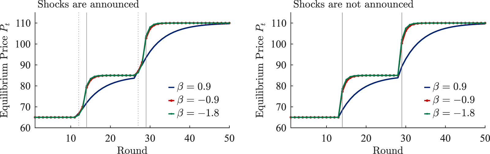


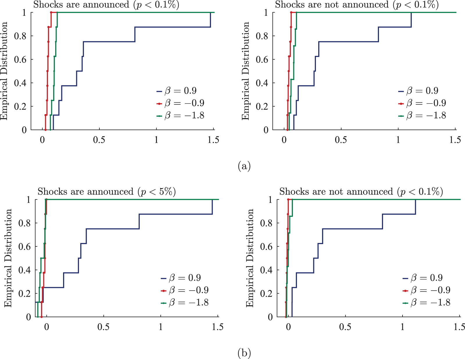
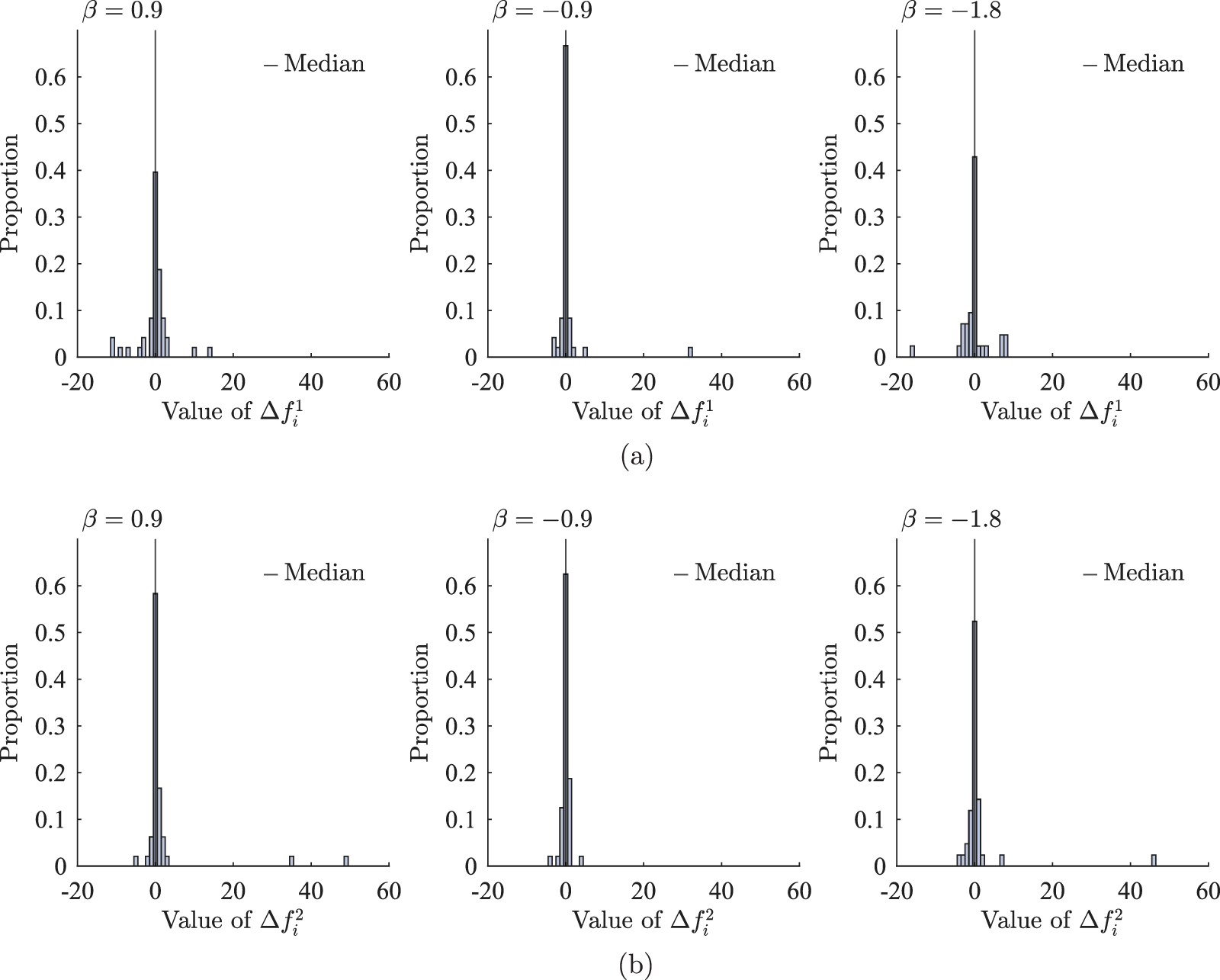


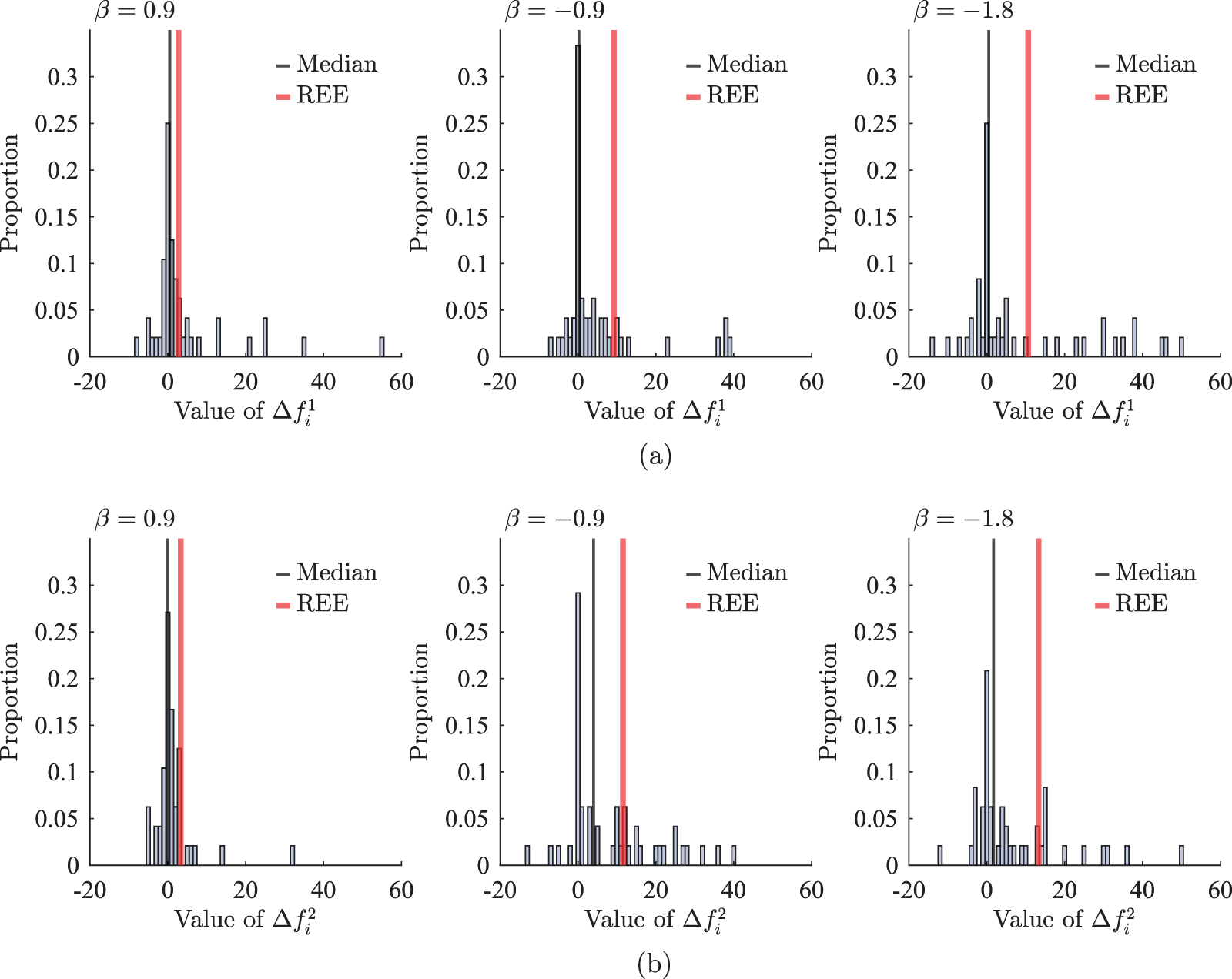


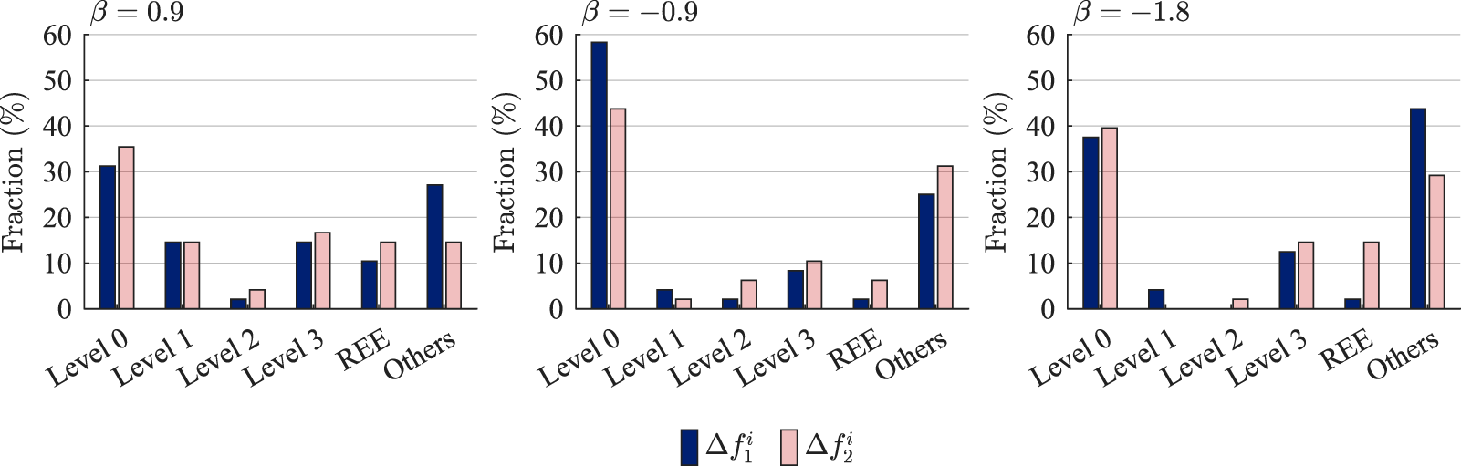


 Open access