






1. Introduction
In this paper, we examine localized patterns for some reaction-diffusion systems driven by saturation or Allee effects. These are often included in population models in order to account for the effect of population size on predation or nutrient consumption. Consider the following variant of the well-known model of mussel–algae interactions [Reference Cangelosi, Wollkind, Kealy-Dichone and Chaiya4, Reference Liu, Weerman, Herman, Olff and van de Koppel27, Reference van de Koppel, Rietkerk, Dankers and Herman25, Reference Wang, Liu, Sun, Jin and van de Koppel42]:
 \begin{equation}
M_{t}=d_{1}M_{xx}-\frac{k_{1}}{k_{2}+M}M+k_{3}AM,\ \ \ \ A_{t}=d_{2}
A_{xx}-VA_{x}+k_{4}-k_{5}A-k_{6}AM.
\end{equation}
\begin{equation}
M_{t}=d_{1}M_{xx}-\frac{k_{1}}{k_{2}+M}M+k_{3}AM,\ \ \ \ A_{t}=d_{2}
A_{xx}-VA_{x}+k_{4}-k_{5}A-k_{6}AM.
\end{equation} The same model but with  $k_{5}=0,V=0,$ was also studied in, e.g. [Reference Ibanez and Velarde14, Reference Peng, Shi and Wang35], from the point of view of chemical reactions with saturation. The mussel death rate
  $\frac{k_{1}
}{k_{2}+M}$ decreases with higher density, reflecting a ‘strength in numbers’ protection mechanism. All parameters are assumed to be positive; see papers [Reference van de Koppel, Rietkerk, Dankers and Herman25, Reference Wang, Liu, Sun, Jin and van de Koppel42] for a detailed explanation of the model and parameters. The path to pattern formation through Turing bifurcation is well understood for this and related models. In particular, the saturation is essential for the formation of spatial patterns in (1.1) (no spatial patterns are possible when saturation
$\frac{k_{1}
}{k_{2}+M}$ decreases with higher density, reflecting a ‘strength in numbers’ protection mechanism. All parameters are assumed to be positive; see papers [Reference van de Koppel, Rietkerk, Dankers and Herman25, Reference Wang, Liu, Sun, Jin and van de Koppel42] for a detailed explanation of the model and parameters. The path to pattern formation through Turing bifurcation is well understood for this and related models. In particular, the saturation is essential for the formation of spatial patterns in (1.1) (no spatial patterns are possible when saturation  $\frac{k_{1}}{k_{2}+M}$ is replaced by $k_{1}$). Our goal here is to study localized patterns that arise far from the Turing bifurcation threshold. This is in contrast to numerous existing studies of this model, where the patterns are typically studied close to the Turing bifurcation threshold.
Many models of vegetation patterns incorporate saturation for both nutrients and plant biomass [Reference Ge11, Reference Guttal and Jayaprakash13, Reference Rietkerk, Boerlijst, Van Langevelde, HilleRisLambers, v. de Koppel, Kumar, Prins and de Roos37]. Among the simplest examples, consider the following variant of the classical Klausmeier model:
 \begin{equation}
v_{t}=d_{2}v_{xx}-k_{4}v+\frac{k_{5}v}{k_{6}v+k_{7}}vu,\ \ u_{t}=d_{1}
u_{xx}+k_{1}-k_{2}u-k_{3}uv.
\end{equation}
\begin{equation}
v_{t}=d_{2}v_{xx}-k_{4}v+\frac{k_{5}v}{k_{6}v+k_{7}}vu,\ \ u_{t}=d_{1}
u_{xx}+k_{1}-k_{2}u-k_{3}uv.
\end{equation} Here,  $v$ represents the biomass density and $u$ the density of water. The water absorption rate by the plants $\frac{k_{5}v}{k_{6}v+k_{7}}$ is assumed to saturate with increased biomass density.
Both of these models have complex spatial patterns made up of spikes, as illustrated in Figures 1 and 5. We are interested in certain limits of the models (1.2) and (1.1) where the saturation plays a key role. As with most other studies of spike patterns, the basic building block is the asymptotic profile of the spike. In almost all other studies, this profile satisfies a nonlinear ODE of the form  $w^{\prime\prime}-w+w^{p}=0$. By contrast, when saturation dominates, we find a new linear ODE for the ground state in the inner region, of the form $w^{\prime\prime}+w-1=0.$ This is then matched to the outer region to construct the full spike profile.
As we will see later, saturation can have a profound effect on the resulting spatial patterns. The original paper of Klausmeier [Reference Klausmeier17] assumed no saturation (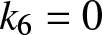 $k_{6}=0$ in (1.2); though the Klausmeier model also included drift terms such as $u_{x}$ in the equation for $u$ to account for the flow of water downhill, which we are not considering here). In this case, the model (1.2) is equivalent to the Gray–Scott model or the Schnakenberg model (when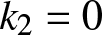 $k_{2}=0$) which has been intensively studied from the point of view of localized patterns. There is a large literature on the subject; we refer to the book [Reference Wei and Winter45] and references therein for review.
Similar localized patterns have been studied in many other reaction-diffusion models. Some prominent examples include the Gray–Scott model [Reference Doelman, Kaper and Zegeling9, Reference Kolokolnikov, Ward and Wei20, Reference Muratov29, Reference Nishiura and Ueyama32, Reference Pearson34, Reference Reynolds, Ponce-Dawson and Pearson36], the Schnakenberg model [Reference Benson, Maini and Sherratt3, Reference Iron, Wei and Winter16, Reference Kolokolnikov and Wei23], vegetation patches in arid environments [Reference Chen, Kolokolnikov, Tzou and Gai7, Reference Gai and Kolokolnikov10, Reference Klausmeier17, Reference Saadi, Champneys, Gai and Kolokolnikov38–Reference Sherratt40], crime hot-spots in a model of residential burglaries [Reference Chaturapruek, Breslau, Yazdi, Kolokolnikov and McCalla5, Reference Kolokolnikov, Ward and Wei22, Reference Short, Dorsogna, Pasour, Tita, Brantingham, Bertozzi and Chayes41, Reference Zipkin, Short and Bertozzi46] and animal skin patterns [Reference Barrio, Varea, Aragón and Maini2, Reference Grall and Tschopp12, Reference Kondo and Asai24, Reference Landge, Jordan, Diego and Müller26, Reference Maini, Woolley, Baker, Gaffney and Lee28, Reference Nogare and Chitnis33]. We single out the paper [Reference Iron, Ward and Wei15], which is the first to give the full description of stability of  $N$ spikes for the related Gierer–Meinhardt model. The framework developed in that paper forms the basis for stability analysis in this work.
The summary of the paper is as follows. Section 2 is dedicated to the analysis of the model (1.1). We construct the equilibrium spike profile in Section 2.1. We then study the stability of a pattern consisting of  $N$ identical copies of a spike in Section 2.2. As in the classical analysis [Reference Iron, Ward and Wei15], there are two types of eigenvalues to consider: large eigenvalues which correspond to structural stability of the pattern, and small eigenvalues that arise due to translation invariance of the inner region and are related to slow spike dynamics. We find a novel non-local eigenvalue problem (NLEP) (3.1) which describes the stability of spikes with respect to large eigenvalues, and proves their (in)stability depending on problem parameters. We then derive small-eigenvalue instability thresholds directly, by constructing asymmetric spike patterns. As with other models, we find that the competition instability – responsible for spike disintegration – is triggered due to small eigenvalue instabilities. In Section 2.3, we derive the so-called core problem, which captures the spike self-replication observed in (1.1). The stability of NLEP problem is analysed rigorously in Section 3. Section 4 is devoted to a similar analysis for the model (1.2). We conclude with a discussion and open problems in Section 5.
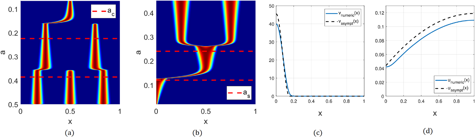
(a) Spike competition instability for the model (2.3). Here,  $D=1,\ \varepsilon=0.0015$, and $a$ is gradually decreased according to $a=0.5-10^{-5}t.$ The number of spikes decreases as $a$ decreases. Dashed line $a_{c}$ shows the asymptotic threshold given by (2.5). Colouration is normalized at each time slice, with deep red corresponding to a maximum and deep blue corresponding to zero. (b) Self-replication. Parameters are the same as in (a) except $a$ is gradually increased according to $a=0.02+10^{-5}t.$ The number of spikes increases as $a$ increases. Asymptotic value for $a_{s}$ given by (2.4) is also shown. (c) and (d) Half-spike steady state of (2.4), which is a basic building block of patterns. Here, $a=0.15,\ \varepsilon=0.01,\ l=1,D=1$. Panel (c) shows $v(x)$ and panel (d) shows $u(x).$ Dashed lines indicate asymptotics (2.15).

Figure 1 Long description
The image A shows a graph with x-axis labeled 'x' and y-axis labeled 'a', depicting spike patterns with varying 'a' values. Dashed lines indicate specific thresholds. The image B shows another graph with similar axes, illustrating different spike patterns with altered 'a' values. The image C presents a line graph with x-axis 'x' and y-axis 'value', showing a decreasing trend with two plotted lines labeled 'v(x)' and 'asymptotic'. The image D displays a line graph with x-axis 'x' and y-axis 'value', showing an increasing trend with two plotted lines labeled 'u(x)' and 'asymptotic'.
2. Mussel–algae model
We illustrate our technique on the mussel–algae model (1.1). Simulations of the steady state (see Figure 1) show the existence of spike patterns, corresponding to localized concentrations of the mussel population. We will first non-dimensionalize equations (1.1) as follows. Let  $M=k_{2}v;\ A=\frac{k_{1}}{k_{2}k_{3}
}u;\ \ t=\frac{k_{2}}{k_{1}}{\tilde{t}}.$ After dropping the tilde we obtain
$M=k_{2}v;\ A=\frac{k_{1}}{k_{2}k_{3}
}u;\ \ t=\frac{k_{2}}{k_{1}}{\tilde{t}}.$ After dropping the tilde we obtain
 \begin{equation}
v_{t}=\varepsilon^{2}v_{xx}+uv-\frac{v}{1+v};\ \ \ \tau u_{t}=Du_{xx}-D_{2}u_{x}+a-bu-uv
\end{equation}
\begin{equation}
v_{t}=\varepsilon^{2}v_{xx}+uv-\frac{v}{1+v};\ \ \ \tau u_{t}=Du_{xx}-D_{2}u_{x}+a-bu-uv
\end{equation}where
 \begin{equation}
a=\frac{k_{4}k_{3}}{k_{1}k_{6}},\ \ b=\frac{k_{5}}{k_{6}k_{2}},\ \ \tau
=\frac{k_{1}}{k_{2}k_{6}k_{2}},\ \ D=\frac{d_{2}}{k_{6}k_{2}},\ \ V_{u}
=\frac{V}{k_{6}k_{2}},\ \ \varepsilon=\sqrt{\frac{d_{1}k_{2}}{k_{1}}}.
\end{equation}
\begin{equation}
a=\frac{k_{4}k_{3}}{k_{1}k_{6}},\ \ b=\frac{k_{5}}{k_{6}k_{2}},\ \ \tau
=\frac{k_{1}}{k_{2}k_{6}k_{2}},\ \ D=\frac{d_{2}}{k_{6}k_{2}},\ \ V_{u}
=\frac{V}{k_{6}k_{2}},\ \ \varepsilon=\sqrt{\frac{d_{1}k_{2}}{k_{1}}}.
\end{equation} In particular, the parameters used in [Reference van de Koppel, Rietkerk, Dankers and Herman25, Reference Wang, Liu, Sun, Jin and van de Koppel42] yield the values  $\varepsilon=0.158,\ \ D_{2}
=360,\ D=0,$
$\varepsilon=0.158,\ \ D_{2}
=360,\ D=0,$  $\tau=0.000131,\ a=0.7,\ \ b=0.6666.$
To simplify the calculation and illustrate key points, we will only look at the regime where the natural death rate of algae is negligible compared to death due to mussel consumption, and take  $b=0$. In addition, we will assume no drift: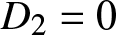 $D_{2}=0$. Note, however, our analysis can be extended to remove these assumptions. Moreover, we assume that the algae population changes on a faster timescale than the mussel population: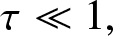 $\tau\ll1,$ consistent with parameters in [Reference van de Koppel, Rietkerk, Dankers and Herman25, Reference Wang, Liu, Sun, Jin and van de Koppel42] (which give $\tau=0.000131$). With these assumptions, we write the simplified model in the form
 \begin{equation}
v_{t}=\varepsilon^{2}v_{xx}+uv-\frac{v}{1+v};\ \ \ 0=Du_{xx}+a-uv.
\end{equation}
\begin{equation}
v_{t}=\varepsilon^{2}v_{xx}+uv-\frac{v}{1+v};\ \ \ 0=Du_{xx}+a-uv.
\end{equation} We will also assume that the ratio of diffusion coefficients  $\varepsilon^{2}/D$ is small; in other words, the mussels move much slower than the algae. This is biologically reasonable, consistent with parameters as given, for example, in [Reference van de Koppel, Rietkerk, Dankers and Herman25, Reference Wang, Liu, Sun, Jin and van de Koppel42] (there, drift $u_{x}$ was used instead of the diffusion $u_{xx}$ here; but very similar analysis is possible in that case), and allows for the decoupling of the spatial scales for $v$ and $u.$
$u.$
2.1. Steady state
Let us first construct a steady state for the model (2.3) asymptotically. It satisfies
 \begin{equation}
0=\varepsilon^{2}v_{xx}+uv-\frac{v}{1+v};\ \ \ 0=Du_{xx}+a-uv.
\end{equation}
\begin{equation}
0=\varepsilon^{2}v_{xx}+uv-\frac{v}{1+v};\ \ \ 0=Du_{xx}+a-uv.
\end{equation} We remark that the equations for the steady state are the same even when  $\tau$ is not assumed to be zero in (2.3); however non-zero $\tau$ complicates the analysis of stability and is a subject of future work. A typical steady state is shown in Figure 1 (c and d). We start by constructing a steady state consisting of a half-spike on the domain
  $\left[
0,l\right] .$ By even reflections, this can be extended to
$\left[
0,l\right] .$ By even reflections, this can be extended to  $N$ symmetric interior spikes on the domain $\left( -l,(2N-1)l\right) $ of size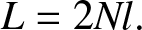 $L=2Nl.$
The steady state is divided into two regions: the inner region inside the spike and the outer region (refer to Figure 1 (c and d)). The analysis is done separately in both regions, along with asymptotic matching to resolve for unsolved constants.
In the inner region, we look for a solution of the form
 \begin{equation}
y=\frac{\sqrt{u_{0}}}{\varepsilon}x,\text{\ }v=\frac{1}{u_{0}}
V(y),\ \ \ u(x)=U(y)
\end{equation}
\begin{equation}
y=\frac{\sqrt{u_{0}}}{\varepsilon}x,\text{\ }v=\frac{1}{u_{0}}
V(y),\ \ \ u(x)=U(y)
\end{equation}where 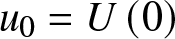 $u_{0}=U\left( 0\right) $ is the value of $u(x)$ at the centre of the spike to be determined. Equation for $U(y)$, at leading order, becomes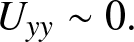 $U_{yy}\sim0.$ It follows that $U(y)\sim u_{0}+By$. Standard asymptotic matching requires that $U(y)$ remains bounded as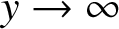 $y\rightarrow\infty$, so that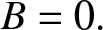 $B=0.$ It follows that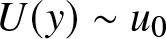 $U(y)\sim u_{0}$ is constant (with $u_{0}$ to be determined) in the inner region to leading order (note that $u(x)$ itself is non-constant, it is only constant to leading order inside the inner region).
Equation for  $V(y)$ then becomes
 \begin{equation}
V_{yy}+V-\frac{V}{u_{0}+V}=0.
\end{equation}
\begin{equation}
V_{yy}+V-\frac{V}{u_{0}+V}=0.
\end{equation} Multiplying by  $V_{y}$ and integrating we obtain
 \begin{equation}
\frac{V_{y}^{2}}{2}+\frac{V^{2}}{2}-V+u_{0}\log(V+u_{0})=C.
\end{equation}
\begin{equation}
\frac{V_{y}^{2}}{2}+\frac{V^{2}}{2}-V+u_{0}\log(V+u_{0})=C.
\end{equation} Assuming that 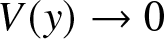 $V(y)\rightarrow0$ as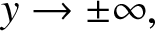 $y\rightarrow\pm\infty,$ we obtain $C=u_{0}\log(u_{0})$ so that (2.7) becomes
 \begin{equation}
\frac{V_{y}^{2}}{2}+\frac{V^{2}}{2}-V+u_{0}\log(V/u_{0}+1)=0.
\end{equation}
\begin{equation}
\frac{V_{y}^{2}}{2}+\frac{V^{2}}{2}-V+u_{0}\log(V/u_{0}+1)=0.
\end{equation} By assumption,  $v(x)$ is symmetric with respect to $x=0$, so that $V(y)$ has a maximum $V_{\max}$ at $y=0,$ $\ V_{\max}=V(0).$ Then $V_{\max}$ satisfies
 \begin{equation}
\frac{V_{\max}^{2}}{2}-V_{\max}+u_{0}\log(V_{\max}/u_{0}+1)=0.
\end{equation}
\begin{equation}
\frac{V_{\max}^{2}}{2}-V_{\max}+u_{0}\log(V_{\max}/u_{0}+1)=0.
\end{equation} We are interested in the limit 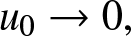 $u_{0}\rightarrow0,$ which we assume to be true throughout this construction. This will impose certain self-consistency conditions on other parameters that will become clear below when $u_{0}$ is solved for below through matching (see (2.13) and (2.16 )). Then (2.9) simplifies to
 \begin{equation}
\frac{V_{\max}^{2}}{2}-V_{\max}\sim0,
\end{equation}
\begin{equation}
\frac{V_{\max}^{2}}{2}-V_{\max}\sim0,
\end{equation}so that 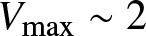 $V_{\max}\sim2$ as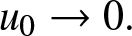 $u_{0}\rightarrow0.$ Furthermore, in the limit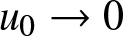 $u_{0}\rightarrow0$, the original equation (2.6) becomes
 \begin{equation}
V_{yy}+V-1\sim0
\end{equation}
\begin{equation}
V_{yy}+V-1\sim0
\end{equation} Consequently, we obtain  $V\sim1+A\cos(y).$ Moreover, $V(0)=V_{\max}=2=1+A$; this yields $V\sim1+\cos(y).$ The approximation (2.11) breaks down when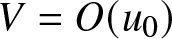 $V=O(u_{0})$, in other words, when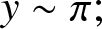 $y\sim\pi;$ an additional boundary layer near $y=\pi$ exists to resolve the transition from (2.11) to (2.6 ).Footnote 1
Finally, in the outer, we assume that  $u$ and $v$ are both small (which imposes a further constraint on parameter $a$ to be determined, see below); the leading order for (2.4) then reads
  $\varepsilon^{2}
v_{xx}-v\sim0$ so that
$\varepsilon^{2}
v_{xx}-v\sim0$ so that  $v$ exhibits a fast exponential decay. Subsequently, to leading order, we obtain the spike profile of the form
 \begin{equation}
v(x)\sim\frac{1}{u_{0}}\left\{
\begin{array}
[c]{c}
1+\cos\left( \frac{\sqrt{u_{0}}}{\varepsilon}x\right) ,\ \ 0\leq x \lt \pi
\frac{\varepsilon}{\sqrt{u_{0}}}\\
0,\ \ \text{otherwise}
\end{array}
\right. .
\end{equation}
\begin{equation}
v(x)\sim\frac{1}{u_{0}}\left\{
\begin{array}
[c]{c}
1+\cos\left( \frac{\sqrt{u_{0}}}{\varepsilon}x\right) ,\ \ 0\leq x \lt \pi
\frac{\varepsilon}{\sqrt{u_{0}}}\\
0,\ \ \text{otherwise}
\end{array}
\right. .
\end{equation} Finally, to obtain  $u_{0},$ we integrate equation for $u$ in (2.3 ) to obtain
  $al\sim u_{0}\int_{0}^{l}vdx\sim\frac{\varepsilon}{\sqrt{u_{0}}
}\pi$ (where
$al\sim u_{0}\int_{0}^{l}vdx\sim\frac{\varepsilon}{\sqrt{u_{0}}
}\pi$ (where  $l$ the distance between the minimum and maximum of $v,$ for example $l=1$ in Figure 2(a)), so that
 \begin{equation}
u_{0}\sim\left( \frac{\varepsilon\pi}{la}\right) ^{2}.
\end{equation}
\begin{equation}
u_{0}\sim\left( \frac{\varepsilon\pi}{la}\right) ^{2}.
\end{equation} In the outer region,  $v\sim0,$ so that $u$ satisfies: $Du_{xx}-a\sim0.$ Matching with the inner region, we have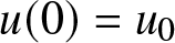 $u(0)=u_{0}$. It follows that
 \begin{equation}
u\sim u_{0}-\frac{a}{2D}\left( \left( x-l\right) ^{2}-l^{2}\right) .
\end{equation}
\begin{equation}
u\sim u_{0}-\frac{a}{2D}\left( \left( x-l\right) ^{2}-l^{2}\right) .
\end{equation} In summary, the half-spike on domain  $\left[ 0,l\right] $ has the profile
 \begin{equation}
\ \ v(x)\sim\left( \frac{al}{\varepsilon\pi}\right) ^{2}\left\{
\begin{array}
[c]{c}
1+\cos\left( \frac{\pi}{al}x\right) ,\ \ 0\leq x \lt al\\
0,\ \ \text{otherwise}
\end{array}
\right. ;\ \ \ \ \ u(x)\sim\left( \frac{\varepsilon\pi}{la}\right)
^{2}-\frac{a}{2D}\left( x-l\right) .
\end{equation}
\begin{equation}
\ \ v(x)\sim\left( \frac{al}{\varepsilon\pi}\right) ^{2}\left\{
\begin{array}
[c]{c}
1+\cos\left( \frac{\pi}{al}x\right) ,\ \ 0\leq x \lt al\\
0,\ \ \text{otherwise}
\end{array}
\right. ;\ \ \ \ \ u(x)\sim\left( \frac{\varepsilon\pi}{la}\right)
^{2}-\frac{a}{2D}\left( x-l\right) .
\end{equation} The assumption  $v\gg1$ and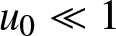 $u_{0}\ll1$ then implies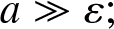 $a\gg\varepsilon;$ at the same time for the spike to be localized we must also have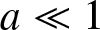 $a\ll1$. In short, the above asymptotic construction is valid provided that:
 \begin{equation}
0 \lt \varepsilon\ll a\ll1,
\end{equation}
\begin{equation}
0 \lt \varepsilon\ll a\ll1,
\end{equation}with other parameters ( $D$ and $l$) being $O(1).$ In fact, as we will show in Section 2.2, critical stability thresholds occur when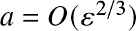 $a=O(\varepsilon^{2/3})$ which is consistent with (2.16). Figure 1 (c and d) shows the comparison between the asymptotics (2.15) and the full steady state as obtained by numerical simulations.
2.2. Stability
Half-spike. We start by studying the stability of a single boundary half-spike on domain of size  $\left( 0,l\right) .$ Linearize around the steady state constructed above as follows:
 \begin{equation*}
v(x,t)=v(x)+\phi(x)e^{\lambda t},\ \ u(x,t)=u(x)+\psi(x)e^{\lambda t}
\end{equation*}
\begin{equation*}
v(x,t)=v(x)+\phi(x)e^{\lambda t},\ \ u(x,t)=u(x)+\psi(x)e^{\lambda t}
\end{equation*}to obtain
 \begin{equation}
\lambda\phi=\varepsilon^{2}\phi_{xx}+\phi u+\psi v-\left( \frac{1}
{1+v}\right) ^{2}\phi;\ \ \ \ 0=D\psi_{xx}-\phi u-\psi v.
\end{equation}
\begin{equation}
\lambda\phi=\varepsilon^{2}\phi_{xx}+\phi u+\psi v-\left( \frac{1}
{1+v}\right) ^{2}\phi;\ \ \ \ 0=D\psi_{xx}-\phi u-\psi v.
\end{equation} In the inner region 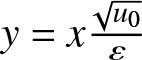 $y=x\frac{\sqrt{u_{0}}}{\varepsilon}$ we approximate $\psi\sim\psi_{0}=\psi(0),\ \ \phi(x)=\Phi(y)$ and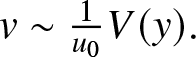 $v\sim\frac{1}{u_{0}}V(y).$ We obtain,
 \begin{equation}
\lambda_{0}\Phi\sim\Phi_{yy}+\Phi+\frac{V}{u_{0}^{2}}\psi_{0},\ \ \ \lambda
_{0}=\lambda/u_{0}\text{,\ }V(y)=1+\cos y,\ \ y\in\left[ 0,\pi\right] .
\end{equation}
\begin{equation}
\lambda_{0}\Phi\sim\Phi_{yy}+\Phi+\frac{V}{u_{0}^{2}}\psi_{0},\ \ \ \lambda
_{0}=\lambda/u_{0}\text{,\ }V(y)=1+\cos y,\ \ y\in\left[ 0,\pi\right] .
\end{equation} To match the outer solution where  $\phi\sim0$, we impose a point constraint
 \begin{equation*}
\Phi\left( \pi\right) =0.
\end{equation*}
\begin{equation*}
\Phi\left( \pi\right) =0.
\end{equation*} We integrate the equation for  $\psi$ in (2.17) to obtain $\psi_{0}:$
 \begin{equation*}
\psi_{0}\sim-\frac{u_{0}^{2}}{\pi}\int_{0}^{\pi}\Phi(y)dy.
\end{equation*}
\begin{equation*}
\psi_{0}\sim-\frac{u_{0}^{2}}{\pi}\int_{0}^{\pi}\Phi(y)dy.
\end{equation*}This yields the following non-local eigenvalue problem (NLEP):
 \begin{equation}
\left\{
\begin{array}
[c]{c}
\lambda_{0}\Phi=\Phi_{yy}+\Phi-\kappa\left( 1+\cos y\right) \int_{0}^{\pi
}\Phi(y)dy,\\
\Phi^{\prime}(0)=0;\ \ \ \ \ \Phi(\pi)=0.
\end{array}
\right.
\end{equation}
\begin{equation}
\left\{
\begin{array}
[c]{c}
\lambda_{0}\Phi=\Phi_{yy}+\Phi-\kappa\left( 1+\cos y\right) \int_{0}^{\pi
}\Phi(y)dy,\\
\Phi^{\prime}(0)=0;\ \ \ \ \ \Phi(\pi)=0.
\end{array}
\right.
\end{equation}where 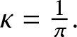 $\kappa=\frac{1}{\pi}.$ The problem (2.19) is studied rigorously in Section 3. In particular, Theorem 3.1 states that the eigenvalues are stable ( $\operatorname{Re}\left( \lambda_{0}\right) \leq0$ for all $\lambda_{0}$) as long as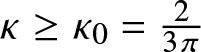 $\kappa\geq\kappa_{0}=\frac{2}{3\pi}$, and are unstable otherwise. Here,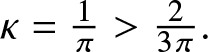 $\kappa=\frac{1}{\pi} \gt \frac{2}{3\pi}.$ This proves that a single boundary spike is stable.
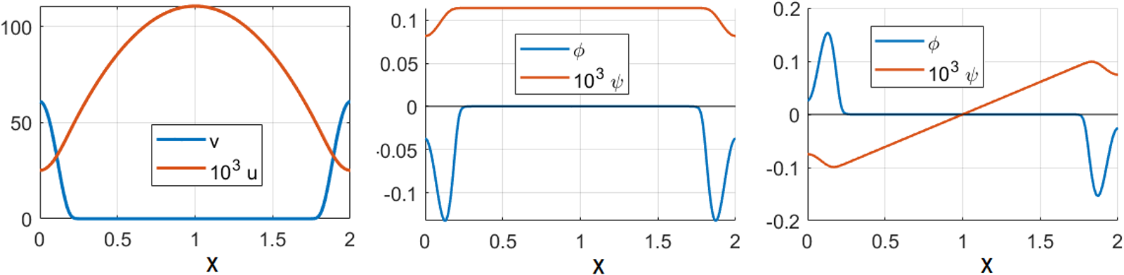
Two boundary spikes. Next, consider the configuration consisting of two boundaries on the domain  $[0,2l]$ as illustrated in Figure 2. This configuration admits two distinct eigenvalues, depending on the parity of the eigenfunction with respect to the centre of the domain, as illustrated in Figure 2. If the eigenfunction is even with respect to the centre, this is equivalent to the stability of a single half-spike on the domain $[0,l]$ and was shown to be stable. On the other hand, an odd eigenfunction is equivalent to solving the eigenvalue problem (2.17 ) with boundary conditions
  $\psi\left( \pm l\right) =0=\phi\left( \pm
l\right) .$ The inner problem for
$\psi\left( \pm l\right) =0=\phi\left( \pm
l\right) .$ The inner problem for  $\Phi$ is the same (2.19); but now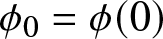 $\phi_{0}=\phi(0)$ satisfies
 \begin{equation*}
\psi_{xx}=0;\ \ \ \ \psi\left( l\right) =0,\ \ D\psi^{\prime}(0^{+}
)=\frac{\varepsilon}{\sqrt{u_{0}}}\left( u_{0}\int_{0}^{\pi}\Phi dy+\psi
_{0}\frac{\pi}{u_{0}}\right)
\end{equation*}
\begin{equation*}
\psi_{xx}=0;\ \ \ \ \psi\left( l\right) =0,\ \ D\psi^{\prime}(0^{+}
)=\frac{\varepsilon}{\sqrt{u_{0}}}\left( u_{0}\int_{0}^{\pi}\Phi dy+\psi
_{0}\frac{\pi}{u_{0}}\right)
\end{equation*} We obtain  $\psi(x)=\psi^{\prime}(0)\left( x-l\right) ,\ \ \psi_{0}\sim
-l\psi^{\prime}(0^{+})$ so that
$\psi(x)=\psi^{\prime}(0)\left( x-l\right) ,\ \ \psi_{0}\sim
-l\psi^{\prime}(0^{+})$ so that
 \begin{equation}
\psi_{0}=-l^{2}\frac{a}{D\pi}\left( u_{0}\int_{0}^{\pi}\Phi dy+\psi_{0}
\frac{\pi}{u_{0}}\right) .
\end{equation}
\begin{equation}
\psi_{0}=-l^{2}\frac{a}{D\pi}\left( u_{0}\int_{0}^{\pi}\Phi dy+\psi_{0}
\frac{\pi}{u_{0}}\right) .
\end{equation}We then obtain the problem (2.19) but with
 \begin{equation}
\kappa=\frac{1}{\pi}\frac{D^{-1}l^{4}a^{3}\left( \varepsilon\pi\right)
^{-2}}{1+D^{-1}l^{4}a^{3}\left( \varepsilon\pi\right) ^{-2}}.
\end{equation}
\begin{equation}
\kappa=\frac{1}{\pi}\frac{D^{-1}l^{4}a^{3}\left( \varepsilon\pi\right)
^{-2}}{1+D^{-1}l^{4}a^{3}\left( \varepsilon\pi\right) ^{-2}}.
\end{equation} The stability boundary corresponds to setting 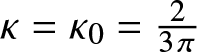 $\kappa=\kappa_{0}=\frac{2}
{3\pi}$, corresponding to the threshold
$\kappa=\kappa_{0}=\frac{2}
{3\pi}$, corresponding to the threshold  $D^{-1}l^{4}a^{3}\left(
\varepsilon\pi\right) ^{-2}=2,$ or
$D^{-1}l^{4}a^{3}\left(
\varepsilon\pi\right) ^{-2}=2,$ or 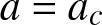 $a=a_{c}$ where
 \begin{equation}
a_{c}=\varepsilon^{2/3}D^{1/3}l^{-4/3}2^{1/3}\pi^{2/3}.
\end{equation}
\begin{equation}
a_{c}=\varepsilon^{2/3}D^{1/3}l^{-4/3}2^{1/3}\pi^{2/3}.
\end{equation} By Theorem 3.1, when 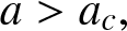 $a \gt a_{c},$ the two boundary spikes are stable, and they are unstable when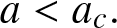 $a \lt a_{c}.$
Left: Steady state consisting of two boundary spikes. Here,  $A=0.2,\ \varepsilon=0.01,\ D=1$ and domain size is $[0,2]$ (correspondingly, $l=1$ is the distance between the maximum and the minimum of a spike). Middle: even eigenfunction corresponding to BC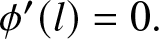 $\phi^{\prime}(l)=0.$ Right: odd eigenfunction corresponding to BC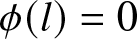 $\phi(l)=0$.

Figure 2 Long description
The image consists of three line graphs. The first graph shows two curves labeled v and 10 superscript 3 u plotted against x, ranging from 0 to 2. The second graph displays two curves labeled phi and 10 superscript 3 u, also plotted against x from 0 to 2. The third graph features two curves labeled phi and 10 superscript 3 u, plotted against x from 0 to 2, with different scales on the y-axis.
Multiple interior spikes. Next, we consider  $N$ spikes on the domain of size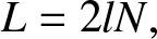 $L=2lN,$ with periodic boundary conditions. We fix the domain $x\in\lbrack-l,(2l-1)N]$ and put the spikes at locations $x=2lk,k=0\ldots N-1$. There are small and large eigenvalues to compute [Reference Iron, Ward and Wei15, Reference Wei and Winter45].
Small eigenvalues. We start with the small eigenvalues that correspond to translational modes. Instead of the full computation of the small eigenvalues, we will short-circuit the process and only compute asymmetric spike solutions following [Reference Kolokolnikov, Ward and Wei22, Reference Ward and Wei43]. The point where the asymmetric branch bifurcates off the symmetric configuration corresponds to the simultaneous zero-crossing of  $N-1$ small eigenvalues [Reference Ward and Wei43].
From (2.15), we have:
 \begin{equation*}
u\left( l\right) \sim u_{0}+\frac{a}{2D}l^{2}\sim\left( \frac
{\varepsilon\pi}{a}\right) ^{2}\frac{1}{l^{2}}+\frac{a}{2D}l^{2}
\end{equation*}
\begin{equation*}
u\left( l\right) \sim u_{0}+\frac{a}{2D}l^{2}\sim\left( \frac
{\varepsilon\pi}{a}\right) ^{2}\frac{1}{l^{2}}+\frac{a}{2D}l^{2}
\end{equation*} The function 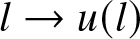 $l\rightarrow u(l)$ attains a minimum when
 \begin{equation*}
-2\left( \frac{\varepsilon\pi}{a}\right) ^{2}\frac{1}{l^{3}}+\frac{a}
{D}l=0.
\end{equation*}
\begin{equation*}
-2\left( \frac{\varepsilon\pi}{a}\right) ^{2}\frac{1}{l^{3}}+\frac{a}
{D}l=0.
\end{equation*} Solving for  $a$, we obtain the same formula as in (2.22). This is precisely the bifurcation point of zero-crossing of small eigenvalues, at which all $N$ small eigenvalues cross zero simultaneously [Reference Ward and Wei43]. This shows that the stability threshold of two interior boundary spikes on domain of size $4l$ (due to small eigenvalues) is exact same as the stability threshold of two boundary spikes on the domain of size $2l$ (due to large eigenvalues). It is notable that the classical systems such as Gierer–Meinhardt or Schnakenberg models exhibit exactly the same equality of stability thresholds. Finally, we let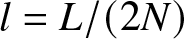 $l=L/(2N)$ to obtain the threshold for $N$ spikes on domain of size $L.$ The small eigenvalues are all stable when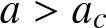 $a \gt a_{c}$ and are all unstable when $a \lt a_{c}.$
Large eigenvalues. To compute large eigenvalues on the periodic domain, we consider the eigenvalue problem (2.17) but subject to the ‘Floquet’ boundary conditions:
 \begin{equation*}
\psi(l)=e^{i\theta}\psi(-l),\ \ \psi^{\prime}(l)=e^{i\theta}\psi^{\prime}(-l)
\end{equation*}
\begin{equation*}
\psi(l)=e^{i\theta}\psi(-l),\ \ \psi^{\prime}(l)=e^{i\theta}\psi^{\prime}(-l)
\end{equation*}and similar for  $\phi.$ Extend $\psi$ on the entire domain by setting $\psi(x)=e^{i\theta}\psi(x-2l)$. Then $\psi((2l-1)N)=e^{i\theta N}\psi(-l).$ By choosing
 \begin{equation*}
\theta=2\pi m/N,\ \ m=0\ldots N-1,
\end{equation*}
\begin{equation*}
\theta=2\pi m/N,\ \ m=0\ldots N-1,
\end{equation*}we obtain periodic boundary conditions on the entire domain. It remains to solve for  $\psi_{0}.$ This is equivalent to solving
 \begin{equation}
\left\{
\begin{array}
[c]{c}
\psi^{\prime\prime}=c\boldsymbol{\delta}(x)\\
\psi(l)=e^{i\theta}\psi(-l),\ \ \psi^{\prime}(l)=e^{i\theta}\psi^{\prime}(-l)
\end{array}
\right.
\end{equation}
\begin{equation}
\left\{
\begin{array}
[c]{c}
\psi^{\prime\prime}=c\boldsymbol{\delta}(x)\\
\psi(l)=e^{i\theta}\psi(-l),\ \ \psi^{\prime}(l)=e^{i\theta}\psi^{\prime}(-l)
\end{array}
\right.
\end{equation}where  $\boldsymbol{\delta}(x)$ is the delta function and
 \begin{equation*}
c=2l\frac{a}{D\pi}\left( u_{0}\int_{0}^{\pi}\Phi dy+\psi_{0}\frac{\pi}{u_{0}
}\right)
\end{equation*}
\begin{equation*}
c=2l\frac{a}{D\pi}\left( u_{0}\int_{0}^{\pi}\Phi dy+\psi_{0}\frac{\pi}{u_{0}
}\right)
\end{equation*} This is equivalent to solving 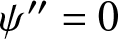 $\psi^{\prime\prime}=0$ with jump condition $\psi^{\prime}(0^{+})-\psi^{\prime}(0^{-})=c$ and continuity condition $\psi(0^{+})=\psi(0^{-}).$ After some algebra we find that
 \begin{equation}
\psi(0)=\frac{cl}{\cos\left( \theta\right) -1}=-\frac{cl}{2\sin^{2}
(\theta/2)}.
\end{equation}
\begin{equation}
\psi(0)=\frac{cl}{\cos\left( \theta\right) -1}=-\frac{cl}{2\sin^{2}
(\theta/2)}.
\end{equation} We then obtain (2.19) with the premultiplier  $\kappa$ being equal to
 \begin{equation}
\kappa=\frac{1}{\pi}\frac{\left( D\sin^{2}(\theta/2)\right) ^{-1}l^{4}
a^{3}\left( \varepsilon\pi\right) ^{-2}}{1+\left( D\sin^{2}(\theta
/2)\right) ^{-1}l^{4}a^{3}\left( \varepsilon\pi\right) ^{-2}}.
\end{equation}
\begin{equation}
\kappa=\frac{1}{\pi}\frac{\left( D\sin^{2}(\theta/2)\right) ^{-1}l^{4}
a^{3}\left( \varepsilon\pi\right) ^{-2}}{1+\left( D\sin^{2}(\theta
/2)\right) ^{-1}l^{4}a^{3}\left( \varepsilon\pi\right) ^{-2}}.
\end{equation} Setting 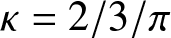 $\kappa=2/3/\pi$ yields the critical threshold
 \begin{equation}
a_{m}=a_{c}\sin^{2/3}\left( \frac{2\pi m}{N}\right) .
\end{equation}
\begin{equation}
a_{m}=a_{c}\sin^{2/3}\left( \frac{2\pi m}{N}\right) .
\end{equation}where  $a_{c}$ is given in (2.5). Note that $a_{m}\leq a_{c}$ for all $m$, so that all of the thresholds $a_{m}$ are below the threshold $a_{c}$ that triggers the small eigenvalues. In this sense, the situation is the same as for the Schnakenberg and other related models: the instability is first triggered by small eigenvalues, as $a$ is decreased.
2.3. Self-replication
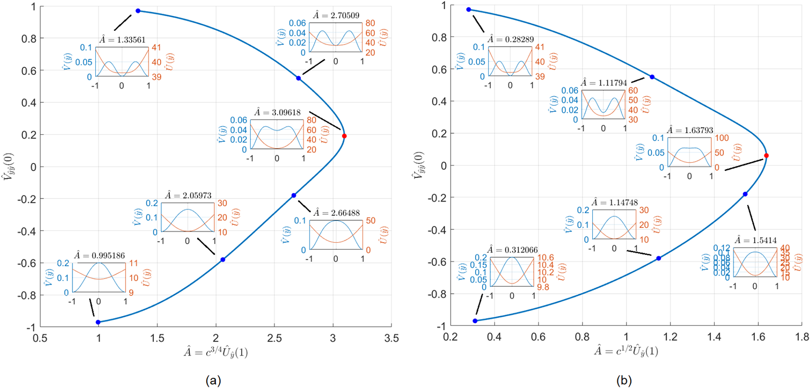
(a) Bifurcation diagram for the core problem (2.29). There is a fold point at  $\hat {A}=\hat{A}_{s}=3.0918$ which is responsible for self-replication. (b) Bifurcation diagram for the core problem (4.10). The fold point is at $\hat{A}=\hat{A}_{s}=1.6379$.

Figure 3 Long description
The image shows two bifurcation diagrams labeled (a) and (b). Diagram (a) plots V subscript yy left parenthesis 0 right parenthesis on the y-axis and A hat equals c superscript 3 over 4 U hat subscript y hat left parenthesis 1 right parenthesis on the x-axis, ranging from 0 to 3.5. It includes insets of waveforms at specific points: A hat equals 1.2285, 1.6379, 2.2096 and 3.0962. Diagram (b) plots V subscript yy left parenthesis 0 right parenthesis on the y-axis and A hat equals c superscript 3 over 4 U hat subscript y hat left parenthesis 1 right parenthesis on the x-axis, ranging from 0.2 to 1.6. It includes insets of waveforms at specific points: A hat equals 0.6360, 1.0918, 1.5144 and 1.6379. Both diagrams illustrate fold points and self-replication phenomena, with arrows indicating transitions between states.
Next, we study the phenomenon of spike self-replication. This phenomenon is observed in numerous other reaction-diffusion models. See for example [Reference Chen and Kolokolnikov6, Reference Doelman, Kaper and Peletier8, Reference Kolokolnikov and Tlidi18, Reference Kolokolnikov, Ward and Wei20, Reference Kolokolnikov, Ward and Wei21, Reference Muratov and Osipov30–Reference Nishiura and Ueyama32, Reference Pearson34, Reference Reynolds, Ponce-Dawson and Pearson36] and references therein. The path to self-replication corresponds to a disappearance of the steady state via a fold-point bifurcation [Reference Nishiura and Ueyama31]. At the bifurcation point, there is typically the so-called ‘core problem’ [Reference Doelman, Kaper and Peletier8, Reference Kolokolnikov, Ward and Wei20, Reference Muratov and Osipov30, Reference Pearson34] near the spike centre, which must be solved numerically, then matched to the outer region. Near the fold point, the solution branch connects a single spike to a double-spike structure. As we now show, a similar structure (but with a somewhat different core problem) occurs for model (2.9).
We start by looking at the inner region of the spike located at  $x=0.$ Rescale:
 \begin{equation*}
x=ay,\ \ u=\varepsilon^{2}a^{-2}U,\ \ \ v=\varepsilon^{-2}a^{2}V,\ \ \ D_{0}
=D\varepsilon^{2}a^{-4}.
\end{equation*}
\begin{equation*}
x=ay,\ \ u=\varepsilon^{2}a^{-2}U,\ \ \ v=\varepsilon^{-2}a^{2}V,\ \ \ D_{0}
=D\varepsilon^{2}a^{-4}.
\end{equation*} Assuming  $v$ large, the leading-order inner problem becomes
 \begin{equation}
V_{yy}-1+UV=0,\ \ \ \ D_{0}U_{yy}-UV\sim0.
\end{equation}
\begin{equation}
V_{yy}-1+UV=0,\ \ \ \ D_{0}U_{yy}-UV\sim0.
\end{equation} The inner problem for  $V(y)$ is defined for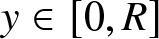 $y\in\lbrack0,R]$ where $R$ is the inner domain length that is necessary to solve for. In order to match the outer region, we impose boundary conditions
 \begin{equation*}
V^{\prime}(0)=0=U^{\prime}(0);\ \ \ V(R)=0=V^{\prime}(R);
\end{equation*}
\begin{equation*}
V^{\prime}(0)=0=U^{\prime}(0);\ \ \ V(R)=0=V^{\prime}(R);
\end{equation*} The matching condition is obtained by integrating the equation for  $U$ in (2.27). We have:
  $U^{\prime}(R)=\frac{1}{D_{0}}\int_{0}^{R}
UVdy\sim\frac{1}{aD_{0}}\int_{0}^{l}uvdx.$ On the other hand, integrating (2.30) we have
$U^{\prime}(R)=\frac{1}{D_{0}}\int_{0}^{R}
UVdy\sim\frac{1}{aD_{0}}\int_{0}^{l}uvdx.$ On the other hand, integrating (2.30) we have 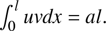 $\int_{0}^{l}uvdx=al.$ We thus obtain the matching condition
 \begin{equation}
U_{y}(\infty)=l/D_{0}.
\end{equation}
\begin{equation}
U_{y}(\infty)=l/D_{0}.
\end{equation} Together, equations (2.27, 2.28) form a closed system that determines  $V,U$ as well as $R$ as a function of system parameters. Next, we further scale to remove $R$ as follows:
 \begin{equation*}
y=R\hat{y},\ \ V=R^{2}\hat{V},\ \ U=R^{-2}\hat{U}
\end{equation*}
\begin{equation*}
y=R\hat{y},\ \ V=R^{2}\hat{V},\ \ U=R^{-2}\hat{U}
\end{equation*}to arrive at the problem
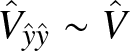
 \begin{equation}
\hat{V}_{yy}-1+\hat{U}\hat{V}=0,\ \ c\hat{U}_{\hat{y}\hat{y}}-\hat{U}\hat{V}=0
\end{equation}
\begin{equation}
\hat{V}_{yy}-1+\hat{U}\hat{V}=0,\ \ c\hat{U}_{\hat{y}\hat{y}}-\hat{U}\hat{V}=0
\end{equation} where  $c=D\varepsilon^{2}a^{-4}R^{-4}.$ The boundary conditions become
 \begin{equation}
\hat{V}^{\prime}(0)=0=\hat{U}^{\prime}(0);\ \ \ \hat{V}(1)=0=\hat{V}^{\prime
}(1).
\end{equation}
\begin{equation}
\hat{V}^{\prime}(0)=0=\hat{U}^{\prime}(0);\ \ \ \hat{V}(1)=0=\hat{V}^{\prime
}(1).
\end{equation} Condition (2.28) then becomes  $\hat{U}_{\hat{y}}(1)=R^{3}l/D_{0}.$ Eliminating $R,$ we get
  $\hat{U}_{\hat{y}}(1)=c^{-3/4}lD^{-1/4}
\varepsilon^{-1/2}a.$
$\hat{U}_{\hat{y}}(1)=c^{-3/4}lD^{-1/4}
\varepsilon^{-1/2}a.$
Let 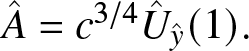 $\hat{A}=c^{3/4}\hat{U}_{\hat{y}}(1).$ The matching then becomes
 \begin{equation}
\hat{A}:=c^{3/4}\hat{U}_{\hat{y}}(1)=lD^{-1/4}\varepsilon^{-1/2}a.
\end{equation}
\begin{equation}
\hat{A}:=c^{3/4}\hat{U}_{\hat{y}}(1)=lD^{-1/4}\varepsilon^{-1/2}a.
\end{equation} $\hat{A}=\hat{A}_{s}\approx3.0962.$ This is illustrated in Figure 3(a), where we plot $\hat{A}$ versus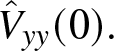 $\hat{V}_{yy}(0).$ The two branches connect a single spike to a double spike solution and are responsible for the self-replication observed in the numerics. When $\hat{A}$ is increased past $\hat{A}_{s}$, the steady state is lost, and self-replication occurs.
We summarize the results as follows.
Proposition 2.1. Consider a symmetric  $N-$spike pattern for the model (2.29) on the domain of size $L,$ and let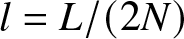 $l=L/(2N)$. Let
 \begin{equation}
a_{s} =\varepsilon^{1/2}D^{1/4}l^{-1}\hat{A}_{s} \ \text{where }\hat{A}
_{s}\approx3.0962,
\end{equation}
\begin{equation}
a_{s} =\varepsilon^{1/2}D^{1/4}l^{-1}\hat{A}_{s} \ \text{where }\hat{A}
_{s}\approx3.0962,
\end{equation} \begin{equation}
a_{c} =\varepsilon^{2/3}D^{1/3}l^{-4/3}2^{1/3}\pi^{2/3}.
\end{equation}
\begin{equation}
a_{c} =\varepsilon^{2/3}D^{1/3}l^{-4/3}2^{1/3}\pi^{2/3}.
\end{equation} When 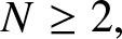 $N\geq2,$ the $N-$spike pattern is stable when
  $a\in\left( a_{c}
,a_{s}\right) .$ Self-replication is triggered when
$a\in\left( a_{c}
,a_{s}\right) .$ Self-replication is triggered when  $a$ increases past $a_{s}$ and competition (spike death) is triggered when $a$ decreases past $a_{c}$. When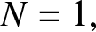 $N=1,$ a single spike is stable when $\varepsilon\ll a \lt a_{s}.$
3. Nonlocal eigenvalue problem
Here, we rigorously study the stability of the key NLEP problem (2.19):
 \begin{equation}
\left\{
\begin{array}
[c]{c}
\lambda_{0}\Phi=\Phi_{yy}+\Phi-\kappa w\int_{0}^{\pi}\Phi
(y)dy,\ \ \ \ \ w(y)=1+\cos(y)\\
\Phi^{\prime}(0)=0;\ \ \ \ \ \Phi(\pi)=0.
\end{array}
\right.
\end{equation}
\begin{equation}
\left\{
\begin{array}
[c]{c}
\lambda_{0}\Phi=\Phi_{yy}+\Phi-\kappa w\int_{0}^{\pi}\Phi
(y)dy,\ \ \ \ \ w(y)=1+\cos(y)\\
\Phi^{\prime}(0)=0;\ \ \ \ \ \Phi(\pi)=0.
\end{array}
\right.
\end{equation}We have the following characterization of stability for the operator (3.1).
Theorem 3.1. Let 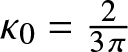 $\kappa_{0}=\frac{2}{3\pi}$. The following thresholds phenomenon holds:
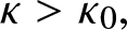
• If $\kappa \gt \kappa_{0},$ then all eigenvalues of (3.1) are strictly stable, i.e.
$\operatorname{Re}\left( \lambda_{0}\right) \lt 0$ for all
$\lambda_{0}$.
$\kappa \gt \kappa_{0},$ then all eigenvalues of (3.1) are strictly stable, i.e.
$\operatorname{Re}\left( \lambda_{0}\right) \lt 0$ for all
$\lambda_{0}$.• If
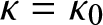
$\kappa=\kappa_{0}$, then there exists one zero eigenvalue and the rest of eigenvalues are strictly stable,
$\operatorname{Re}\left( \lambda
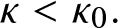
_{0}\right) \lt 0.$• Suppose that
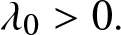
$\kappa \lt \kappa_{0}.$ Then there exists a real positive eigenvalue
$\lambda_{0} \gt 0.$



Note that the operator in (3.1) is not self-adjoint and in general the eigenvalues can be complex, which complicates the analysis. We will follow the ideas of the method introduced in [Reference Wei44]. The idea is to ‘self-adjointize’ the operator.
In what follows, we write 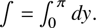 $\int=\int_{0}^{\pi}dy.$ Let $w_{0}$, $\kappa_{0}$ be the solution to (3.1) corresponding to the zero eigenvalue, namely
 \begin{equation*}
w_{0}^{\prime\prime}+w_{0}-\kappa_{0}w\int w_{0}=0.
\end{equation*}
\begin{equation*}
w_{0}^{\prime\prime}+w_{0}-\kappa_{0}w\int w_{0}=0.
\end{equation*}Explicitly, we have
 \begin{equation*}
w_{0}(y)=\cos y+1+\frac{1}{2}y\sin y;\ \ \ \kappa_{0}=\frac{1}{\int w_{0}
}=\frac{2}{3\pi}.
\end{equation*}
\begin{equation*}
w_{0}(y)=\cos y+1+\frac{1}{2}y\sin y;\ \ \ \kappa_{0}=\frac{1}{\int w_{0}
}=\frac{2}{3\pi}.
\end{equation*}Now define the operator
 \begin{equation}
L_{1}\Phi:=\Phi^{\prime\prime}+\Phi-\kappa_{0}w\int\Phi-\kappa_{0}\int
w\Phi+\kappa_{1}\int\Phi
\end{equation}
\begin{equation}
L_{1}\Phi:=\Phi^{\prime\prime}+\Phi-\kappa_{0}w\int\Phi-\kappa_{0}\int
w\Phi+\kappa_{1}\int\Phi
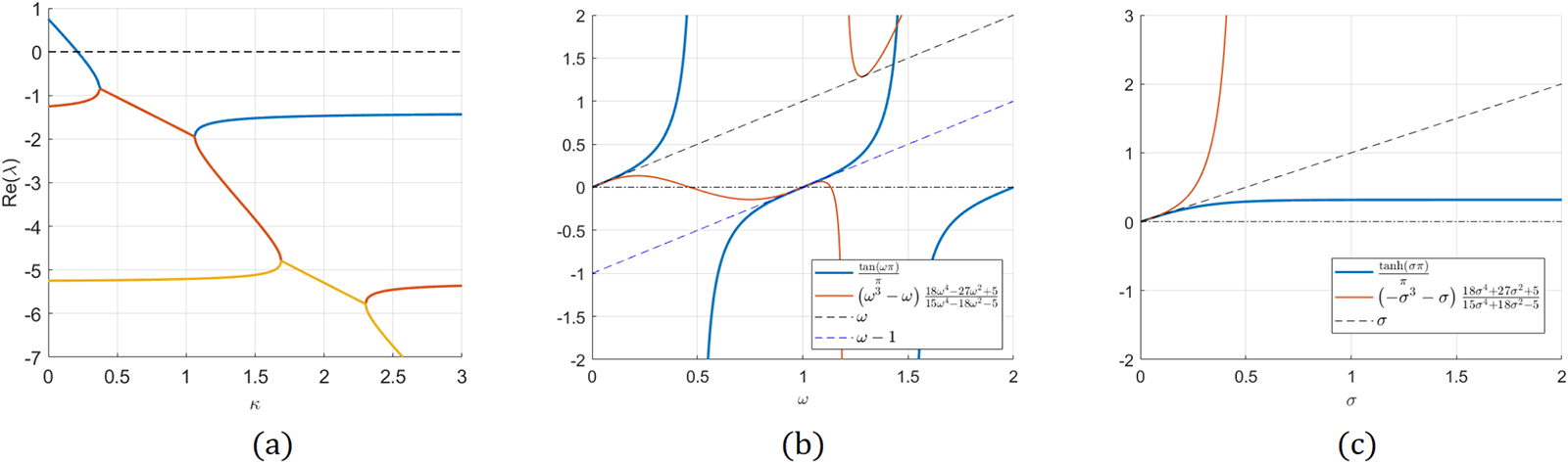
\end{equation}(a) Spectrum of the eigenvalue problem (3.1) computed numerically. Note the zero-crossing at 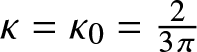 $\kappa=\kappa_{0}=\frac{2}{3\pi}$ of the principal eigenvalue. The problem is stable for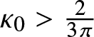 $\kappa_{0} \gt \frac{2}{3\pi }$, despite having complex eigenvalues. (b) Plot of (3.3). (c) Plot of (3.4).

Figure 4 Long description
The image A shows a graph with the x-axis labeled kappa and the y-axis labeled real part of lambda. It features curves intersecting at various points, with one curve crossing the zero line. The image B shows a graph with the x-axis labeled omega and the y-axis labeled real part of lambda. It includes multiple curves, with one labeled as lhs of equation 3.3 and another as rhs of equation 3.3. The image C shows a graph with the x-axis labeled omega and the y-axis labeled real part of lambda, displaying a single curve with a steep incline. Each graph has distinct axes and curves, illustrating different mathematical relationships.
where  $\kappa_{1}$ is chosen such that $L_{1}w_{0}=0:$
 \begin{align*}
0 & =-\kappa_{0}\int ww_{0}+\kappa_{1}\int w_{0},\\
\kappa_{1} & =\kappa_{0}\frac{\int ww_{0}}{\int w_{0}}=\frac{5}{6\pi}.
\end{align*}
\begin{align*}
0 & =-\kappa_{0}\int ww_{0}+\kappa_{1}\int w_{0},\\
\kappa_{1} & =\kappa_{0}\frac{\int ww_{0}}{\int w_{0}}=\frac{5}{6\pi}.
\end{align*}Lemma 3.2. The operator  $L_{1}$ is self-adjoint and non-positive definite.
Proof. An explicit computation shows that the eigenvalues of  $L_{1}$ satisfy
 \begin{equation}
\frac{\tan\left( \omega\pi\right) }{\pi}=\left( \omega^{3}-\omega\right)
\frac{18\omega^{4}-27\omega^{2}+5}{15\omega^{4}-18\omega^{2}-5},\ \ \ \lambda
=1-\omega^{2}
\end{equation}
\begin{equation}
\frac{\tan\left( \omega\pi\right) }{\pi}=\left( \omega^{3}-\omega\right)
\frac{18\omega^{4}-27\omega^{2}+5}{15\omega^{4}-18\omega^{2}-5},\ \ \ \lambda
=1-\omega^{2}
\end{equation} Since  $L_{1}$ is self-adjoint, $\lambda$ is purely real. So there are two cases to consider: either $\omega$ is purely real or it is purely imaginary.
Case 1,  $\omega$ is purely real. The graph of lhs and rhs of (3.3) is shown in Figure 4(b). As can be seen from the graph, there are no roots when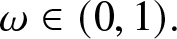 $\omega\in(0,1).$ This is easy to prove rigorously as follows. Let $f(\omega)=rhs(3.3).$ Then for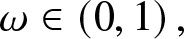 $\omega\in\left( 0,1\right) ,$ $f(\omega)$ is below the line $y=\omega$ and above the line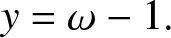 $y=\omega-1.$ Indeed, a simple computation shows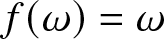 $f(\omega)=\omega$ is equivalent
 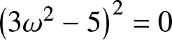 $\left(
3\omega^{2}-5\right) ^{2}=0$ which has no roots in
$\left(
3\omega^{2}-5\right) ^{2}=0$ which has no roots in 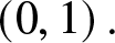 $\left( 0,1\right) .$ Similarly, setting $f(w)=\omega-1$ one obtains
  $18\omega^{4}+54\omega
^{3}+48\omega^{2}+15\omega+5=0$, which again has no roots for
$18\omega^{4}+54\omega
^{3}+48\omega^{2}+15\omega+5=0$, which again has no roots for 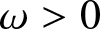 $\omega \gt 0$ as all the coefficients are positive.
Case 2, 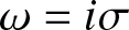 $\omega=i\sigma$ with $\sigma$ purely real. Then equation (3.3) becomes
 \begin{equation}
\frac{\tanh\left( \sigma\pi\right) }{\pi}=\left( -\sigma^{3}-\sigma\right)
\frac{18\sigma^{4}+27\sigma^{2}+5}{15\sigma^{4}+18\sigma^{2}-5}
\end{equation}
\begin{equation}
\frac{\tanh\left( \sigma\pi\right) }{\pi}=\left( -\sigma^{3}-\sigma\right)
\frac{18\sigma^{4}+27\sigma^{2}+5}{15\sigma^{4}+18\sigma^{2}-5}
\end{equation}The graph of (3.4) is shown in Figure 4(c) and shows that there are no non-zero solutions to (3.4). This is easily shown using the same arguments as in Case 1 (and is left to the reader). This completes the proof of the lemma.
We are now ready to prove Theorem 3.1.
Proof of Theorem 3.1
To show the instability when 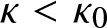 $\kappa \lt \kappa_{0}$, we solve (3.1 ) explicitly to find that $\lambda_{0}$ satisfies
 \begin{equation}
\frac{\tan\left( \omega\pi\right) }{\pi\left( \omega-\omega^{3}\right)
}=1-\frac{\omega^{2}}{\kappa\pi},\ \ \lambda_{0}=1-\omega^{2}.
\end{equation}
\begin{equation}
\frac{\tan\left( \omega\pi\right) }{\pi\left( \omega-\omega^{3}\right)
}=1-\frac{\omega^{2}}{\kappa\pi},\ \ \lambda_{0}=1-\omega^{2}.
\end{equation} Simple calclulus shows that (3.5) has a root 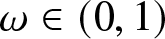 $\omega\in\left(
0,1\right) $ when
$\omega\in\left(
0,1\right) $ when 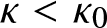 $\kappa \lt \kappa_{0}$ (in fact $\omega=1$ corresponds to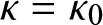 $\kappa=\kappa_{0}$). This shows the existence of a positive (and real) eigenvalue of (3.1) when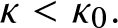 $\kappa \lt \kappa_{0}.$
Next, we show stability when 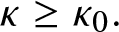 $\kappa\geq\kappa_{0}.$ Write (3.1) as
 \begin{equation*}
\lambda_{0}\Phi=L_{1}\Phi+\left( \kappa_{0}-\kappa\right) w\int\Phi
+\kappa_{0}\int w\Phi-\kappa_{1}\int\Phi
\end{equation*}
\begin{equation*}
\lambda_{0}\Phi=L_{1}\Phi+\left( \kappa_{0}-\kappa\right) w\int\Phi
+\kappa_{0}\int w\Phi-\kappa_{1}\int\Phi
\end{equation*} Decompose  $\lambda_{0}=\lambda_{R}+i\lambda_{I},\ \ \Phi=\Phi_{R}+i\Phi_{I};$ so that
 \begin{equation}
\lambda_{R}\Phi_{R}-\lambda_{I}\Phi_{I} =L_{1}\Phi_{R}+\left( \kappa
_{0}-\kappa\right) w\int\Phi_{R}+\kappa_{0}\int w\Phi_{R}-\kappa_{1}\int
\Phi_{R}
\end{equation}
\begin{equation}
\lambda_{R}\Phi_{R}-\lambda_{I}\Phi_{I} =L_{1}\Phi_{R}+\left( \kappa
_{0}-\kappa\right) w\int\Phi_{R}+\kappa_{0}\int w\Phi_{R}-\kappa_{1}\int
\Phi_{R}
\end{equation} \begin{equation}
\lambda_{R}\Phi_{I}+\lambda_{I}\Phi_{R} =L_{1}\Phi_{I}+\left( \kappa
_{0}-\kappa\right) w\int\Phi_{I}+\kappa_{0}\int w\Phi_{I}-\kappa_{1}\int
\Phi_{I}
\end{equation}
\begin{equation}
\lambda_{R}\Phi_{I}+\lambda_{I}\Phi_{R} =L_{1}\Phi_{I}+\left( \kappa
_{0}-\kappa\right) w\int\Phi_{I}+\kappa_{0}\int w\Phi_{I}-\kappa_{1}\int
\Phi_{I}
\end{equation} The combination  $\int\Phi_{R}\int(3.6)+\int\Phi_{I}\int(3.7)$ yields:
 \begin{align}\lambda_{R}\left\{ \left( \int\Phi_{R}\right) ^{2}+\left( \int\Phi
_{I}\right) ^{2}\right\} & =\left\{ \int\Phi_{R}L_{1}\Phi_{R}+\Phi
_{I}L_{1}\Phi_{I}\right\} +\left( \kappa_{0}-\kappa-\kappa_{1}\right)
\pi\left\{ \left( \int\Phi_{R}\right) ^{2}+\left( \int\Phi_{I}\right)
^{2}\right\} \nonumber\\
& \quad +\kappa_{0}\pi\left\{ \int\Phi_{R}w\int\Phi_{R}+\int\Phi_{I}w\int\Phi
_{I}\right\} \end{align}
\begin{align}\lambda_{R}\left\{ \left( \int\Phi_{R}\right) ^{2}+\left( \int\Phi
_{I}\right) ^{2}\right\} & =\left\{ \int\Phi_{R}L_{1}\Phi_{R}+\Phi
_{I}L_{1}\Phi_{I}\right\} +\left( \kappa_{0}-\kappa-\kappa_{1}\right)
\pi\left\{ \left( \int\Phi_{R}\right) ^{2}+\left( \int\Phi_{I}\right)
^{2}\right\} \nonumber\\
& \quad +\kappa_{0}\pi\left\{ \int\Phi_{R}w\int\Phi_{R}+\int\Phi_{I}w\int\Phi
_{I}\right\} \end{align}Note that
 \begin{equation*}
\int w\left( \Phi^{\prime\prime}+\Phi\right) =\int\Phi\left( w^{\prime
\prime}+w\right) =\int\Phi.
\end{equation*}
\begin{equation*}
\int w\left( \Phi^{\prime\prime}+\Phi\right) =\int\Phi\left( w^{\prime
\prime}+w\right) =\int\Phi.
\end{equation*} Multiplying (3.6, 3.7) by  $w$, integrating and eliminating $\lambda_{I}$ therefore yields
 \begin{equation}
\lambda_{R}\left\{ \left( \int w\Phi_{R}\right) ^{2}+\left( \int w\Phi
_{I}\right) ^{2}\right\} =\left( 1-\kappa\int w^{2}\right) \left\{
\int\Phi_{R}w\int\Phi_{R}+\int\Phi_{I}w\int\Phi_{I}\right\} .
\end{equation}
\begin{equation}
\lambda_{R}\left\{ \left( \int w\Phi_{R}\right) ^{2}+\left( \int w\Phi
_{I}\right) ^{2}\right\} =\left( 1-\kappa\int w^{2}\right) \left\{
\int\Phi_{R}w\int\Phi_{R}+\int\Phi_{I}w\int\Phi_{I}\right\} .
\end{equation} Eliminate  $\int w\Phi_{R}\int\Phi_{R}+\int w\Phi_{I}\int\Phi_{I}$ between (3.8) and (3.9) to obtain
 \begin{equation*}
\lambda_{R}\left( A\right) -\kappa_{0}\pi\lambda_{R}B\frac{1}{\left(
1-\kappa\int w^{2}\right) }=\left\{ \int\Phi_{R}L_{1}\Phi_{R}+\Phi_{I}
L_{1}\Phi_{I}\right\} +\left( \kappa_{0}-\kappa-\kappa_{1}\right) \pi A
\end{equation*}
\begin{equation*}
\lambda_{R}\left( A\right) -\kappa_{0}\pi\lambda_{R}B\frac{1}{\left(
1-\kappa\int w^{2}\right) }=\left\{ \int\Phi_{R}L_{1}\Phi_{R}+\Phi_{I}
L_{1}\Phi_{I}\right\} +\left( \kappa_{0}-\kappa-\kappa_{1}\right) \pi A
\end{equation*}where
 \begin{equation*}
A=\left\{ \left( \int\Phi_{R}\right) ^{2}+\left( \int\Phi_{I}\right)
^{2}\right\} ,\ \ \ B=\left\{ \left( \int\Phi_{R}w\right) ^{2}+\left(
\int\Phi_{I}w\right) ^{2}\right\} .
\end{equation*}
\begin{equation*}
A=\left\{ \left( \int\Phi_{R}\right) ^{2}+\left( \int\Phi_{I}\right)
^{2}\right\} ,\ \ \ B=\left\{ \left( \int\Phi_{R}w\right) ^{2}+\left(
\int\Phi_{I}w\right) ^{2}\right\} .
\end{equation*} Using the fact that 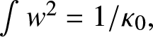 $\int w^{2}=1/\kappa_{0},$ we get
 \begin{equation*}
\lambda_{R}\left( A+\frac{4}{9\pi}\frac{1}{\kappa-\kappa_{0}}B\right)
=\left\{ \int\Phi_{R}L_{1}\Phi_{R}+\Phi_{I}L_{1}\Phi_{I}\right\} +\left(
\kappa_{0}-\kappa-\kappa_{1}\right) \pi A
\end{equation*}
\begin{equation*}
\lambda_{R}\left( A+\frac{4}{9\pi}\frac{1}{\kappa-\kappa_{0}}B\right)
=\left\{ \int\Phi_{R}L_{1}\Phi_{R}+\Phi_{I}L_{1}\Phi_{I}\right\} +\left(
\kappa_{0}-\kappa-\kappa_{1}\right) \pi A
\end{equation*} Now 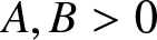 $A,B \gt 0$ whereas the right hand side is always negative when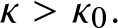 $\kappa \gt \kappa_{0}.$ This shows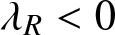 $\lambda_{R} \lt 0$ whenever
  $\kappa \gt \kappa
_{0}.\ \blacksquare$
$\kappa \gt \kappa
_{0}.\ \blacksquare$
4. Schnakenberg model with saturation
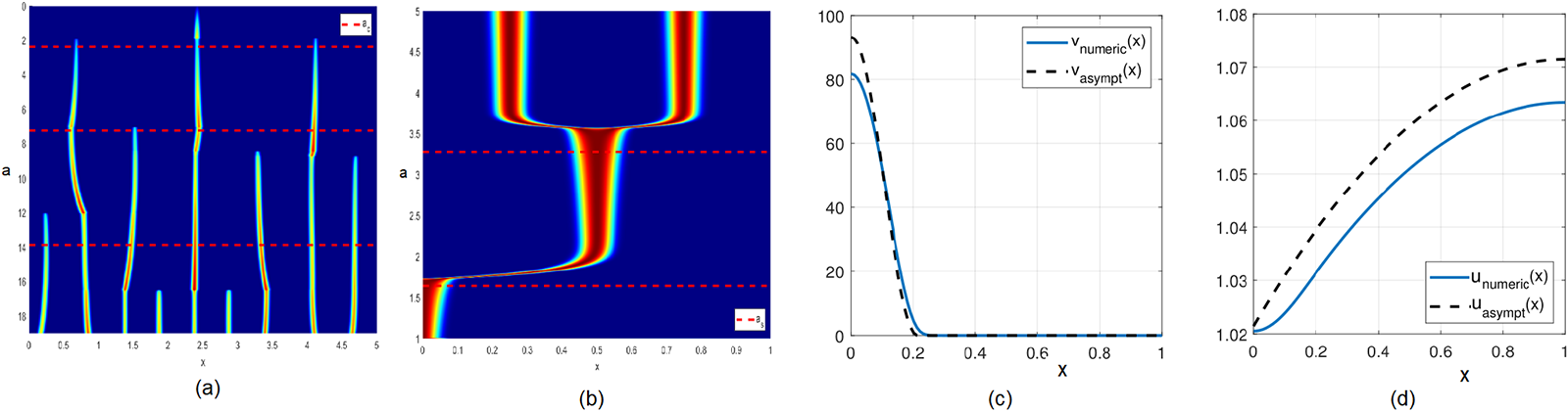
(a) Competition instability for model (4.1). Here,  $D=100,\varepsilon=0.0025$,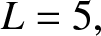 $L=5,$ and $a$ is gradually decreased according to $\ a=20(1-10^{-5}t)$. Dashed lines indicate the asymptotic prediction $a_{c}$ (4.12) for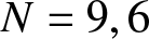 $N=9,6$, and 3 spikes. Colouration is normalized at each time slice, with deep red corresponding to a maximum and deep blue corresponding to zero. (b) Spike self-replication. Here, $D=1,L=1,\varepsilon =0.005$. Dashed lines indicate the asymptotic prediction $a_{s}$ (4.11) for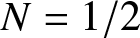 $N=1/2$ and $N=1$ spikes. (c) and (d) Half-spike steady state of (4.1). Panel (c) shows $v$ and panel (d) shows $u$. Here, $D=100,\ a=10,\ \varepsilon=0.01,\ l=1.$ Dashed lines indicate asymptotics (4.2, 4.3, 4.4).

Figure 5 Long description
The image A shows a visual pattern with vertical lines and dashed horizontal lines labeled 'a'. The image B shows a complex pattern with a central narrowing and dashed horizontal lines labeled 'b'. The image C is a line graph with the x-axis labeled 'x' and the y-axis labeled 'value', showing two curves: one solid and one dashed. The image D is another line graph with the x-axis labeled 'x' and the y-axis labeled 'value', also showing two curves: one solid and one dashed.
We now perform a similar analysis for the Schnakenberg model with saturation (1.2). After some scaling, we write it in the form
 \begin{equation}
v_{t}=\varepsilon^{2}v_{xx}-v+\frac{v}{1+v}uv,\ \ \ \ 0=Du_{xx}+a-uv.
\end{equation}
\begin{equation}
v_{t}=\varepsilon^{2}v_{xx}-v+\frac{v}{1+v}uv,\ \ \ \ 0=Du_{xx}+a-uv.
\end{equation} We simplified the model assuming  $k_{2}$ is negligible, and further assumed that the plant population changes on a slower scale than the precipitation in the soil (hence zero instead of $u_{t}$). We first construct the steady state, then analyse its stability.
As before, we will assume that  $u$ and $v$ decouple in the inner region, and start by constructing a single boundary spike on domain
  $\left[ 0,l\right]
.$ In the inner region,
$\left[ 0,l\right]
.$ In the inner region,  $u$ is assumed to be nearly constant, and turns out to be very close to 1, whereas $v$ is large. Setting $u(x)\sim1+\delta$, where $\delta$ is a small constant to be determined, the equilibrium for $v$ becomes
 \begin{equation*}
0=\varepsilon^{2}v_{xx}+\delta v+\left( 1+\delta\right) \left( -1+\frac
{1}{1+v}\right) .
\end{equation*}
\begin{equation*}
0=\varepsilon^{2}v_{xx}+\delta v+\left( 1+\delta\right) \left( -1+\frac
{1}{1+v}\right) .
\end{equation*} Assuming  $v$ large we estimate
  $\left( 1+\delta\right) \left( -1+\frac
{1}{1+v}\right) \sim-1$. We then find, as in Section 2,
$\left( 1+\delta\right) \left( -1+\frac
{1}{1+v}\right) \sim-1$. We then find, as in Section 2,
 \begin{equation}
v(x)\sim\frac{1}{\delta}\left\{
\begin{array}
[c]{c}
\left( 1+\cos\left( x\frac{\sqrt{\delta}}{\varepsilon}\right) \right)
,\ \ \ \left\vert x\right\vert \lt \pi\frac{\varepsilon}{\sqrt{\delta}}\\
0\text{, \ }\left\vert x\right\vert \gt \pi\frac{\varepsilon}{\sqrt{\delta}}
\end{array}
\right.
\end{equation}
\begin{equation}
v(x)\sim\frac{1}{\delta}\left\{
\begin{array}
[c]{c}
\left( 1+\cos\left( x\frac{\sqrt{\delta}}{\varepsilon}\right) \right)
,\ \ \ \left\vert x\right\vert \lt \pi\frac{\varepsilon}{\sqrt{\delta}}\\
0\text{, \ }\left\vert x\right\vert \gt \pi\frac{\varepsilon}{\sqrt{\delta}}
\end{array}
\right.
\end{equation} To find  $\delta,$ we integrate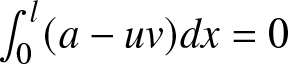 $\int_{0}^{l}(a-uv)dx=0$ which yields
 \begin{equation}
\delta=\varepsilon^{2/3}\left( \frac{\pi}{al}\right) ^{2/3}.
\end{equation}
\begin{equation}
\delta=\varepsilon^{2/3}\left( \frac{\pi}{al}\right) ^{2/3}.
\end{equation}Stability computation is also very similar to Section 2. We compute that
 \begin{equation}
u(x)\sim1+\delta-\frac{a}{2D}\left( x-l\right) ^{2}+\frac{a}{2D}
l^{2},\ \ \ \delta^{2/3}\ll x \lt l
\end{equation}
\begin{equation}
u(x)\sim1+\delta-\frac{a}{2D}\left( x-l\right) ^{2}+\frac{a}{2D}
l^{2},\ \ \ \delta^{2/3}\ll x \lt l
\end{equation}so that
 \begin{equation*}
u(l)=1+\delta+\frac{a}{2D}l^{2}\sim1+\varepsilon^{2/3}\left( \frac{\pi}
{a}\right) ^{2/3}l^{-2/3}+\frac{a}{2D}l^{2}.
\end{equation*}
\begin{equation*}
u(l)=1+\delta+\frac{a}{2D}l^{2}\sim1+\varepsilon^{2/3}\left( \frac{\pi}
{a}\right) ^{2/3}l^{-2/3}+\frac{a}{2D}l^{2}.
\end{equation*} The function 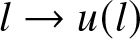 $l\rightarrow u(l)$ attains a minimum when
 \begin{equation}
\frac{2}{3}\varepsilon^{2/3}\left( \frac{\pi}{a}\right) ^{2/3}
l^{-5/3}=2\frac{a}{2D}l.
\end{equation}
\begin{equation}
\frac{2}{3}\varepsilon^{2/3}\left( \frac{\pi}{a}\right) ^{2/3}
l^{-5/3}=2\frac{a}{2D}l.
\end{equation} Solving (4.5) for  $a,$ we obtain the stability threshold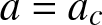 $a=a_{c}$ given by (4.12). The pattern is unstable if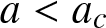 $a \lt a_{c}$ and is is stable for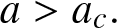 $a \gt a_{c}.$ For large eigenvalues, we linearize around the steady state to obtain the eigenvalue problem
 \begin{equation}
\lambda\phi=\varepsilon^{2}\phi_{xx}+\phi\left( \left( u-1\right) -\frac
{u}{\left( 1+v\right) ^{2}}\right) +\left( -1+v+\frac{1}{1+v}\right)
\psi,\ \ \ \ 0=D\psi_{xx}-\phi u-\psi v.
\end{equation}
\begin{equation}
\lambda\phi=\varepsilon^{2}\phi_{xx}+\phi\left( \left( u-1\right) -\frac
{u}{\left( 1+v\right) ^{2}}\right) +\left( -1+v+\frac{1}{1+v}\right)
\psi,\ \ \ \ 0=D\psi_{xx}-\phi u-\psi v.
\end{equation} The corresponding NLEP problem is identical to (2.19) but with the following  $\kappa:$
 \begin{align*}
\kappa & =\frac{1}{\pi}\varepsilon^{-2/3}\left( \frac{\pi}{al}\right)
^{-2/3}\text{for a single boundary spike on }(0,l)\\[3pt]
\kappa & =\frac{l^{2}a}{D}\frac{1}{\pi}\varepsilon^{-2/3}\left( \frac{\pi
}{al}\right) ^{-2/3}\text{for double boundary spike on }\left( 0,2l\right)
\\[3pt]
\kappa & =\frac{l^{2}a}{D\sin^{2}(\theta/2)}\frac{1}{\pi}\varepsilon
^{-2/3}\left( \frac{\pi}{al}\right) ^{-2/3}\text{,\ \ }m=1\ldots N-1\text{
for }N\text{spikes on domain of size }2lN.
\end{align*}
\begin{align*}
\kappa & =\frac{1}{\pi}\varepsilon^{-2/3}\left( \frac{\pi}{al}\right)
^{-2/3}\text{for a single boundary spike on }(0,l)\\[3pt]
\kappa & =\frac{l^{2}a}{D}\frac{1}{\pi}\varepsilon^{-2/3}\left( \frac{\pi
}{al}\right) ^{-2/3}\text{for double boundary spike on }\left( 0,2l\right)
\\[3pt]
\kappa & =\frac{l^{2}a}{D\sin^{2}(\theta/2)}\frac{1}{\pi}\varepsilon
^{-2/3}\left( \frac{\pi}{al}\right) ^{-2/3}\text{,\ \ }m=1\ldots N-1\text{
for }N\text{spikes on domain of size }2lN.
\end{align*} As before, the stability boundary corresponds to 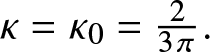 $\kappa=\kappa_{0}=\frac
{2}{3\pi}.$ So no surprise here: we have the usual situation that the small eigenvalues are destabilized before large ones, and therefore (4.12) gives the competition instability threshold.
$\kappa=\kappa_{0}=\frac
{2}{3\pi}.$ So no surprise here: we have the usual situation that the small eigenvalues are destabilized before large ones, and therefore (4.12) gives the competition instability threshold.
Finally, we derive the self-replication thresholds. We rescale,
 \begin{equation*}
u(x)=1+\varepsilon^{2/3}U(y),\ \ \ v(x)=\frac{1}{\varepsilon^{2/3}
}V(y),\ \ \ x=\varepsilon^{2/3}y.
\end{equation*}
\begin{equation*}
u(x)=1+\varepsilon^{2/3}U(y),\ \ \ v(x)=\frac{1}{\varepsilon^{2/3}
}V(y),\ \ \ x=\varepsilon^{2/3}y.
\end{equation*}We then obtain, at leading order, a coupled core problem
 \begin{equation}
V_{yy}+VU-1=0,\ \ \ \ \ DU_{yy}-V=0.
\end{equation}
\begin{equation}
V_{yy}+VU-1=0,\ \ \ \ \ DU_{yy}-V=0.
\end{equation} Similar to (2.1), the inner problem for  $V(y)$ is defined for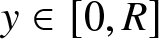 $y\in\lbrack0,R]$ where $R$ is the inner domain length that is necessary to solve for through additional constraints
 \begin{equation}
V^{\prime}(0)=0=U^{\prime}(0)\text{\ \ and \ \ }V(R)=V^{\prime}(R)=0.
\end{equation}
\begin{equation}
V^{\prime}(0)=0=U^{\prime}(0)\text{\ \ and \ \ }V(R)=V^{\prime}(R)=0.
\end{equation} The matching condition is obtained by integrating the equation for  $U$ in (4.7). We have:
  $U^{\prime}(R)=\frac{1}{D}\int_{0}^{R}V(y)dy\sim\frac{1}{D}\int
_{0}^{l}v(x)dx.$ On the other hand, integrating (4.1) we have
$U^{\prime}(R)=\frac{1}{D}\int_{0}^{R}V(y)dy\sim\frac{1}{D}\int
_{0}^{l}v(x)dx.$ On the other hand, integrating (4.1) we have  $\int_{0}^{L}uvdx\sim\int_{0}^{L}vdx=al.$ We thus obtain the matching condition
 \begin{equation}
U^{\prime}(R)=\frac{al}{D}.
\end{equation}
\begin{equation}
U^{\prime}(R)=\frac{al}{D}.
\end{equation} Together, equations (4.7, 4.8, 4.9) form a closed system that determines  $V,U$ as well as $R$ as a function of system parameters. Next, we further scale to remove $R$ as follows:
 \begin{equation*}
y=R\hat{y},\ \ V=R^{2}\hat{V},\ \ U=\frac{1}{R^{2}}\hat{U},\ \ \ c=\frac
{D}{R^{6}}.
\end{equation*}
\begin{equation*}
y=R\hat{y},\ \ V=R^{2}\hat{V},\ \ U=\frac{1}{R^{2}}\hat{U},\ \ \ c=\frac
{D}{R^{6}}.
\end{equation*}The resulting system is
 \begin{equation}
\hat{V}_{\hat{y}\hat{y}}+\hat{V}\hat{U}-1 =0,\ \ \ \ \ c\hat{U}_{\hat
{y}\hat{y}}-\hat{V}=0;
\end{equation}
\begin{equation}
\hat{V}_{\hat{y}\hat{y}}+\hat{V}\hat{U}-1 =0,\ \ \ \ \ c\hat{U}_{\hat
{y}\hat{y}}-\hat{V}=0;
\end{equation} \begin{equation}
\hat{V}^{\prime}(0) =0=\hat{U}^{\prime}(0);\ \ \ \ \hat{V}(1)=\hat
{V}^{\prime}(1)=0
\end{equation}
\begin{equation}
\hat{V}^{\prime}(0) =0=\hat{U}^{\prime}(0);\ \ \ \ \hat{V}(1)=\hat
{V}^{\prime}(1)=0
\end{equation}whereas equation (4.9) becomes
 \begin{equation}
\hat{A}=\hat{U}^{\prime}(1)\sqrt{c},\ \ \ \text{where }\hat{A}=\frac{al}
{\sqrt{D}}.
\end{equation}
\begin{equation}
\hat{A}=\hat{U}^{\prime}(1)\sqrt{c},\ \ \ \text{where }\hat{A}=\frac{al}
{\sqrt{D}}.
\end{equation} $c,$ the system (4.10) is solved numerically. Numerically, we find a fold point at $\hat{A}=\hat{A}_{s}=1.638.$ This is illustrated in Figure 3, where we plot $\hat{A}$ versus
 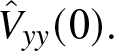 $\hat
{V}_{yy}(0).$ The two branches connect a single spike to a double spike solution and are responsible for the self-replication observed in the numerics.
$\hat
{V}_{yy}(0).$ The two branches connect a single spike to a double spike solution and are responsible for the self-replication observed in the numerics.
We summarize the results as follows.
Theorem 4.1.
Consider a symmetric  $N-$spike pattern for the model (4.1) on the domain of size $L,$ and let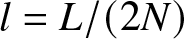 $l=L/(2N)$. Let
 \begin{equation}
a_{s} =D^{1/2}l^{-1}\hat{A}_{\max} \ \text{where }\hat{A}_{s}\approx
1.638,
\end{equation}
\begin{equation}
a_{s} =D^{1/2}l^{-1}\hat{A}_{\max} \ \text{where }\hat{A}_{s}\approx
1.638,
\end{equation} \begin{equation}
a_{c} =D^{3/5}\varepsilon^{2/5}l^{-8/5}(2/3)^{3/5}\pi^{2/5}.
\end{equation}
\begin{equation}
a_{c} =D^{3/5}\varepsilon^{2/5}l^{-8/5}(2/3)^{3/5}\pi^{2/5}.
\end{equation} When 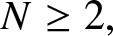 $N\geq2,$ the $N-$spike pattern is stable when
  $a\in\left( a_{c}
,a_{s}\right) .$ Self-replication is triggered when
$a\in\left( a_{c}
,a_{s}\right) .$ Self-replication is triggered when  $a$ increases past $a_{s}$ and competition (spike death) is triggered when $a$ decreases past $a_{c}$. When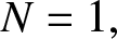 $N=1,$ a single spike is stable when $\varepsilon\ll a \lt a_{s}.$
5. Discussion
We studied the effect of saturation on localized pattern formation for systems (1.1), (1.2). To our knowledge, this is the first time that the asymptotics and stability of localized patterns have been studied for the mussel–algae model 1.1). In contrast to numerous previous studies where the spike have a profile of the form of  $\operatorname{sech}$ to some power, the spike studied here has a cosine-type profile (2.15) and leads to novel NLEP problem (3.1).
Our techniques apply to a wide range of reaction-diffusion systems in the presence of saturation. Another example is a variant of Macarthur–Rosenzweig type model with an Allee effect for the predator, similar to [Reference Akhtar, Peet and Peacock-Lopez1]:
 \begin{equation}
N_{t}=d_{1}N_{xx}+k_{1}N-k_{2}N^{2}-k_{3}NP,\ \ \ \ P_{t}=d_{2}P_{xx}
-k_{4}P+\frac{k_{5}P}{k_{6}P+k_{7}}NP
\end{equation}
\begin{equation}
N_{t}=d_{1}N_{xx}+k_{1}N-k_{2}N^{2}-k_{3}NP,\ \ \ \ P_{t}=d_{2}P_{xx}
-k_{4}P+\frac{k_{5}P}{k_{6}P+k_{7}}NP
\end{equation} Here,  $N$ and $P$ are populations of prey and predator, respectively. The predator-prey interactions are modulated by the predator Allee effect $\frac{k_{5}P}{k_{6}P+k_{7}}$, which allows for spatial pattern formation. It is very similar to the model (1.2) except that the constant production is replaced by a logistic growth term. This makes the outer problem non-linear. It would be interesting to study how this changes the dynamics and stability of localized patterns.
There are numerous open questions for future study. These include: spot dynamics, oscillatory instabilities and construction of stripes and spots in higher dimensions. In two dimensions, we expect the spot profile to be described by a Bessel J function. It would be interesting to extend the stability analysis of Section 2.2 to this context. On the other hand, stable stripe solutions have also been observed in numerical simulations of the mussel–algae model in 2D when the drift terms are added to algae [Reference Liu, Weerman, Herman, Olff and van de Koppel27]. It was shown in [Reference Kolokolnikov, Ward, Tzou and Wei19] that drift can indeed lead to stripe stabilization for the classical Schnakenberg model. It would be interesting to attempt a similar analysis for the mussel–algae model.
Funding statement
S.X. is supported by the NSFC China (Grant No. 12401198).
T.K. is supported by the NSERC Discovery Grant, Canada.
J. Wei is partially supported by the National Key R&D Program of China (No. 2022YFA1005602), and the Hong Kong General Research Fund ‘New frontiers in singular limits of nonlinear partial differential equations’.

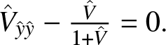

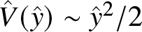
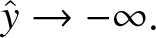

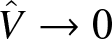












 Open access

