

Impact statement
This study provides clear evidence on the relative effectiveness of key climate policy instruments in OECD countries. The findings show that renewable energy investment delivers significantly stronger and more stable reductions in carbon dioxide emissions than existing environmental tax schemes. While environmental taxes often produce weak or inconsistent effects, renewable energy expansion generates persistent long-term emission reductions across countries. These results have important implications for the allocation of limited public resources and private capital. Policymakers can achieve greater climate impact by prioritizing renewable energy deployment, technological upgrading and energy system integration rather than relying primarily on environmental taxation. The analysis also highlights that emission reductions materialize gradually over time, underscoring the need for stable and forward-looking climate policies. By identifying which policy instruments are most effective, this study supports more targeted climate strategies and contributes to more efficient progress toward long-term decarbonization goals.
Introduction
As climate change intensifies, environmental policy issues worldwide have reached a new level of urgency. Countries are facing the linked difficulties of keeping their economies growing and cutting down on carbon pollution, leading to a renewed focus on how well environmental taxes and the encouragement of renewable energy actually work. The urgency for effective action stems not only from international commitments like the Paris Agreement but also from the tangible consequences of global warming – including rising sea levels, extreme weather events and ecosystem degradation. It is within this context that our study investigates the impact of environmental tax revenue and renewable energy consumption on CO₂ emissions, aiming to provide insights into how these instruments shape environmental outcomes across countries.
Despite growing policy attention to environmental taxation and renewable energy, there is limited empirical consensus on their relative effectiveness in reducing carbon dioxide emissions in advanced economies. Existing studies often report mixed results and rely on single econometric approaches that may fail to capture cross-country heterogeneity, cross-sectional dependence and dynamic adjustment processes. As a result, policymakers face uncertainty when prioritizing climate policy instruments and allocating limited public resources.
At the heart of this research is a fundamental policy question: can economic instruments serve as powerful levers for environmental protection without compromising economic development? Environmental taxes, by internalizing negative externalities, theoretically incentivize polluters to reduce emissions and adopt cleaner technologies. Meanwhile, the expansion of renewable energy offers a pathway toward decarbonizing the energy sector – traditionally the largest source of emissions globally. Yet the effectiveness of these tools remains contested, particularly across different national contexts with varying levels of industrialization, institutional strength and policy enforcement.
A key reason for this uncertainty lies in methodological limitations in existing studies. Many prior analyses employ single-estimator approaches, which, while common, may produce fragile or biased conclusions. Such conventional methods often fail to adequately account for complex issues inherent in panel data, including cross-sectional dependence arising from global economic shocks, heterogeneous dynamics across countries and the distinction between short-run and long-run effects. Moreover, relying solely on one estimator can obscure nuanced patterns, particularly when policy impacts vary by country context or over time. This methodological gap underscores the need for a more robust econometric framework capable of rigorously testing the sensitivity and stability of policy relationships and providing more definitive evidence on the relative efficacy of environmental taxes versus renewable energy support.
Empirical literature has established a robust consensus on the efficacy of environmental taxation and renewable energy in curbing carbon emissions, a finding consistently demonstrated across various methodological frameworks. Seminal studies employing static long-run estimators, such as Doğan et al. (Reference Doğan, Chu, Ghosh, Diep Truong and Balsalobre-Lorente2022) for the G7 and Wolde-Rufael and Mulat-Weldemeskel (Reference Wolde-Rufael and Mulat-Weldemeskel2023) for a European panel, have affirmed this relationship, a conclusion further nuanced by contemporary research which applies dynamic approaches to confirm significant effects in both the short and long run. However, this prevailing consensus rests on findings derived from individual methodological specifications, which cannot attest to their robustness against alternative statistical assumptions. To address this critical limitation and provide a more definitive test, our study advances the methodological frontier by deploying a comprehensive, multi-model econometric framework. This approach, integrating Pooled Mean Group (PMG), Mean Group (MG), Common Correlated Effects Mean Group (CCEMG) and First-Difference Fixed Effects (FD-FE) estimators, is specifically designed to model dynamic adjustment and is uniquely privileged to assess the sensitivity and robustness of the purported relationships. By confronting the existing consensus with this battery of complementary tests, our methodology does not merely replicate prior analyses, but provides a superior basis for evaluating whether established policy effects endure under a broader set of rigorous specifications.
To this end, this study implements a comprehensive, multi-model econometric framework to re-evaluate the joint impact of environmental tax revenue and renewable energy consumption on CO₂ emissions in 16 advanced OECD economies over the period 2000–2022. To capture both immediate and persistent effects, we employ a suite of complementary estimators –FD-FE, PMG, MG and CCEMG – designed to control for heterogeneity, cross-sectional dependence and dynamic adjustment.
Our empirical analysis reveals a critical divergence that challenges the prevailing consensus. While renewable energy consumption emerges as a powerful and reliable driver of emissions reduction, with effects that strengthen substantially from the short run to the long run, environmental tax revenues, as currently designed and implemented, show no statistically significant effect on CO₂ emissions across our sample. This finding indicates that the presumed efficacy of environmental taxes is not robust to more rigorous methodological testing.
This study therefore contributes to the literature in two major ways. First, it provides a methodologically superior assessment that tests the sensitivity of key policy relationships, revealing the fragility of the established link between environmental tax revenue and emissions. Second, it delivers a decisive and practical policy insight for advanced economies: direct renewable energy deployment is a substantially more potent and reliable tool for decarbonization than prevailing carbon pricing mechanisms. This necessitates a re-evaluation of policy priorities and instrument design.
The existing literature on environmental taxation and renewable energy largely evaluates these instruments in isolation or within narrowly specified econometric frameworks. Few studies systematically compare their effectiveness using multiple complementary estimators within a unified framework. This limits the robustness and policy relevance of existing findings, particularly for OECD countries where institutional, technological and economic conditions vary substantially.
This study addresses these limitations by applying a comprehensive multi-model panel econometric framework to examine the effects of renewable energy consumption and environmental tax revenue on carbon dioxide emissions across OECD countries. By employing fixed effects, mean group, pooled mean group and common correlated effects estimators, the analysis captures both short-run and long-run dynamics while accounting for cross-country heterogeneity and unobserved common factors. The study contributes to the literature by providing robust comparative evidence on the relative effectiveness of key climate policy instruments and offers clear guidance for policymakers seeking efficient pathways toward long-term emissions reduction.
Literature review
Addressing the growing environmental crisis has become one of the most significant challenges of the 21st century. Scholars broadly agree that reconciling economic development with environmental protection is not only desirable but also necessary for achieving sustainable growth (World Bank, 2016; Costa-Campi et al., Reference Costa-Campi, del Rio and Trujillo-Baute2017; Landrigan et al., Reference Landrigan, Fuller, Acosta, Adeyi, Arnold, Baldé, Bertollini, Bose-O’Reilly, Boufford and Breysse2018; IPCC, 2022; Wolde-Rufael and Mulat-Weldemeskel, Reference Wolde-Rufael and Mulat-Weldemeskel2023). This urgency is underscored by Landrigan et al. (Reference Landrigan, Fuller, Acosta, Adeyi, Arnold, Baldé, Bertollini, Bose-O’Reilly, Boufford and Breysse2018), who emphasize that pollution is among the most significant existential threats faced by humanity, undermining not only ecological integrity but also economic stability and public health. In line with this, the World Bank (2016) has warned that the health and economic burdens imposed by pollution serve as a “sobering wake-up call,” highlighting the urgent need for policy action. The IPCC (2022) and others (e.g., Tol, Reference Tol2017; Wolde-Rufael and Mulat-Weldemeskel, Reference Wolde-Rufael and Mulat-Weldemeskel2023) further reinforce the imperative to reduce greenhouse gas emissions as a foundational pillar of any credible climate strategy.
To ground these conceptual assertions empirically, Figure A1 reveals divergent national pathways in CO₂ emissions across our sample of 16 OECD countries (2000–2022). While several European states show pronounced declines, others exhibit stable or rising trajectories. These divergent outcomes highlight the critical question of what explains the varied effectiveness of national climate strategies and underscore the need to evaluate the core policy instruments designed to drive decarbonization (See Figures A2, A3).
To understand why some countries reduce emissions faster than others, we examine key policy tools. These include fiscal instruments and technological interventions. Climate policy often focuses on market-based fiscal tools. The most common are carbon taxes and emissions trading schemes. These instruments aim to make polluters pay for environmental costs. They also steer investment toward cleaner energy (Martin et al., Reference Martin, Muûls and Wagner2016; Baranzini et al., Reference Baranzini, Van Den Bergh, Carattini, Howarth, Padilla and Roca2017; Haites, Reference Haites2018). Alongside these, direct promotion of renewable energy is a major technological pathway. A rigorous comparison of these instruments is therefore essential. We must analyze environmental taxation and renewable energy deployment together.
Classical and contemporary environmental economic theory underpins these instruments. Pigouvian logic – originally articulated by Pigou (Reference Pigou2002) – argues for corrective taxes to internalize negative externalities, while Baumol and Oates (Reference Baumol, Oates, Bohm and Kneese1971) refine this tradition by recommending the alignment of environmental taxes with marginal environmental damages. Tol (Reference Tol2017) and the Carbon Pricing Leadership Coalition (Reference Coalition2019) contend that a gradually increasing and globally uniform carbon tax would be among the most efficient mitigation strategies. The OECD (2010) broadens the fiscal taxonomy, distinguishing energy taxes, transport taxes, pollution taxes and resource taxes; comparative studies indicate that carbon-specific taxation often yields stronger mitigation effects than general energy taxes, particularly by stimulating alternative energy adoption (Lin and Li, Reference Lin and Li2011). The EU’s 2030 Climate and Energy Framework – targeting a 40% emissions reduction, a 32% renewable energy share and a 32.5% improvement in energy efficiency – illustrates the synergies between fiscal instruments and sustainable energy transitions (Río, Reference Río2009; European Commission, 2019; Wolde-Rufael and Mulat-Weldemeskel, Reference Wolde-Rufael and Mulat-Weldemeskel2023).
In addition to policy-based instruments, a substantial strand of environmental economics examines the relationship between economic development and environmental pressure through the Environmental Kuznets Curve (EKC) hypothesis (Grossman and Krueger, Reference Grossman and Krueger1995; Dinda, Reference Dinda2004). This framework suggests an inverted U-shaped relationship, where environmental degradation tends to increase with income growth at early stages but may decrease after a certain income level, influenced by structural economic changes, technological progress and growing attention to environmental quality. Empirical support for the EKC remains debated, especially in advanced economies, where reductions in emissions appear to be more strongly associated with active policy interventions, such as environmental taxes and renewable energy programs than with income growth alone (Kaika and Zervas, Reference Kaika and Zervas2013; Stern, Reference Stern2018). Therefore, while the EKC provides a useful reference point for understanding the growth–emission nexus, its relevance in the context of deliberate decarbonization policies requires further empirical study. This research examines the income–emission relationship within a broader model that also considers the role of specific policy instruments, assessing whether EKC patterns are observed or if policy measures play a more decisive role.
Empirical research assessing the efficacy of environmental tax revenue and renewable energy in mitigating CO₂ emissions is growing but yields mixed findings. Doğan et al. (Reference Doğan, Chu, Ghosh, Diep Truong and Balsalobre-Lorente2022) analyze the interplay between environmental taxes and carbon emissions across G7 economies, finding that unsustainable energy practices and ecosystem degradation have amplified climate risks, especially after the COVID-19 shock. Research on environmental taxation more broadly produces heterogeneous results, in part because studies vary in sample composition, estimation strategy and the extent to which they control for structural moderators. Wolde-Rufael and Mulat-Weldemeskel (Reference Wolde-Rufael and Mulat-Weldemeskel2021) examine seven emerging economies and conclude that market-based instruments hold theoretical promise but are underutilized in practice; consequently, their impact on emissions reduction has been limited. These implementation gaps are echoed across the literature, where uneven carbon pricing regimes and continued fossil fuel dependence blunt policy effectiveness (Pigou, Reference Pigou2002; Tol, Reference Tol2013; Haites, Reference Haites2018).
A key explanation for inconsistent empirical outcomes is the mediating influence of structural factors such as environmental technology and financial development. Bashir et al. (Reference Bashir, Ma, Shahbaz and Jiao2020) find that technological advancement and financial maturity significantly modulate the effectiveness of environmental taxes, implying that policy impacts hinge on complementary conditions. Extending this perspective, Dogan et al. (Reference Dogan, Hodžić and Fatur Šikić2022) argue for linking environmental tax rates to ecological thresholds and climate targets – such as the Paris Agreement’s 1.5 °C objective – drawing on both classical Pigouvian theory and modern refinements (Pigou, Reference Pigou2002; Baumol and Oates, Reference Baumol, Oates, Bohm and Kneese1971). In the EU context, Wolde-Rufael and Mulat-Weldemeskel (Reference Wolde-Rufael and Mulat-Weldemeskel2023) underscore the comparative potency of carbon taxes over general energy taxes, stressing the importance of fossil fuel-specific levies. Al Shammre et al. (Reference Al Shammre, Benhamed, Ben-Salha and Jaidi2023) corroborate these nuances in OECD countries, showing that energy taxes – which constitute a large share of environmental tax revenues – are effective in reducing emissions but operate non-linearly, with efficacy conditional on reaching certain thresholds. These findings advocate for nuanced policy design that accounts for technology costs, financial market depth and threshold effects. Furthermore, the rapidly declining cost of key renewable technologies (IRENA, 2024) has enhanced their feasibility, making a robust assessment of their relative performance against fiscal tools all the more urgent.
Empirical literature has established a robust consensus on the efficacy of environmental taxation and renewable energy in curbing carbon emissions, a finding consistently demonstrated across various methodological frameworks. Seminal studies employing static long-run estimators, such as Doğan et al. (Reference Doğan, Chu, Ghosh, Diep Truong and Balsalobre-Lorente2022) for the G7 and Wolde-Rufael and Mulat-Weldemeskel (Reference Wolde-Rufael and Mulat-Weldemeskel2023) for a European panel, have affirmed this relationship, a conclusion further nuanced by contemporary research which applies dynamic approaches to confirm significant effects in both the short and long run. However, this prevailing consensus rests on findings derived from individual methodological specifications, which cannot attest to their robustness against alternative statistical assumptions. To address this critical limitation and provide a more definitive test, our study advances the methodological frontier by deploying a comprehensive, multi-model econometric framework. This approach – integrating PMG, MG, CCEMG and FD-FE estimators – is specifically designed to model dynamic adjustment and is uniquely privileged to assess the sensitivity and robustness of the purported relationships. By confronting the existing consensus with this battery of complementary tests, our methodology does not merely replicate prior analyses but provides a superior basis for evaluating whether established policy effects endure under a broader set of rigorous specifications.
Methodology
Data and sample
This study examines the relationship between renewable energy adoption, environmental taxation and carbon dioxide emissions across 16 OECD countries over the period 2000–2022. The sample comprises a balanced panel dataset with 368 observations (16 countries × 23 years), encompassing Australia, Austria, Denmark, Finland, France, Germany, Italy, Japan, New Zealand, Norway, Portugal, Spain, Sweden, Switzerland, Türkiye and the United Kingdom.
The selection of this sample is strategically designed to balance analytical rigor with policy relevance. It focuses on countries that are policy pioneers in climate action and maintain high-quality, standardized data on environmental taxes and energy statistics through the OECD, which is essential for robust cross-national comparison. The sample captures a spectrum of advanced economies employing varied policy mixes, allowing for a comparative analysis of effectiveness. Furthermore, the intentional inclusion of an emerging economy like Türkiye, characterized by rapid industrialization and significant emission growth, provides a critical contrasting case. This heterogeneity tests whether the identified relationships hold under different developmental pressures, thereby enhancing the external validity of our findings within the OECD context and ensuring they are not solely reflective of a homogenous group of the most advanced economies.
Variable construction and descriptive statistics
Data on CO₂ emissions (MtCO₂), primary energy consumption (Exajoules) and renewable energy consumption (Exajoules) were obtained from the Energy Institute. Environmental tax revenue data (USD millions) were sourced from the OECD Environmental Policy Database, while GDP per capita (current USD) was retrieved from the World Bank’s World Development Indicators (Table 1). All monetary values are expressed in current US dollars to maintain consistency with international reporting standards.
Variable definitions and sources

To address heteroscedasticity and achieve elasticity interpretations, all variables were transformed into natural logarithms. The dependent variable is ln(CO₂), representing log-transformed carbon dioxide emissions. Independent variables include ln(Energy) for total primary energy consumption, ln(RE) for renewable energy consumption, ln(Tax) for environmental tax revenue and ln(GDP) for GDP per capita. Table 2 below summarizes the descriptive statistics.
Descriptive statistics

Note: All variables are natural logarithms. CO₂ = carbon dioxide emissions (MtCO₂); Energy = primary energy consumption (Exajoules); RE = renewable energy consumption (Exajoules); Tax = environmental tax revenue (USD millions); GDP = GDP per capita (current USD). The squared term ln(GDP)2 tests the Environmental Kuznets Curve hypothesis.
The correlation matrix (Table 3) reveals strong positive correlations between CO₂ emissions and both total energy consumption (0.957) and environmental taxation (0.865), suggesting these variables move together over time. Renewable energy shows a weaker positive correlation with CO₂ (0.383), while GDP per capita exhibits a negative correlation (−0.267), potentially indicating decoupling in advanced economies. A visual representation of this correlation matrix for all log-transformed variables is provided in Figure A4.
Correlation matrix

The quadratic term of GDP per capita, ln(GDP)2, is included to test the Environmental Kuznets Curve hypothesis, which posits an inverted U-shaped relationship between economic development and environmental degradation. The high correlation between ln(GDP) and ln(GDP)2 (0.999) is expected in polynomial specifications and does not indicate harmful multicollinearity, as both terms are necessary to capture the hypothesized non-linear relationship.
Hypothesis testing framework
To guide our empirical analysis, we formally specify the following null hypotheses (H₀) concerning the relationships between the key explanatory variables and CO₂ emissions. For GDP per capita, the theoretical relationship is ambiguous: the scale effect of economic growth suggests a positive link, while the EKC hypothesis predicts an inverted U-shaped relationship (non-linear). To empirically distinguish between these possibilities, our model includes both a linear and a quadratic term for GDP per capita. We therefore test a joint null hypothesis for income effects (H₀₄) that both the linear and quadratic terms are zero:
-
• H₀₁: Energy consumption has no significant effect on CO₂ emissions (β₁ = 0).
-
• H₀₂: Renewable energy consumption has no significant effect on CO₂ emissions (β₂ = 0).
-
• H₀₃: Environmental tax revenue has no significant effect on CO₂ emissions (β₃ = 0).
-
• H₀₄: GDP per capita has no significant linear or non-linear effect on CO₂ emissions (β₄ = 0 and β₅ = 0, where β₅ is the coefficient on [ln(GDP)]2).
The corresponding alternative hypotheses (H₁) posit a nonzero effect (βᵢ ≠ 0). For H₀4, the alternative is that at least one of the two coefficients (β₄ or β₅) is nonzero.
These hypotheses are tested across short-run and long-run horizons using our multi-model econometric strategy. The FD-FE model captures short-run elasticities, while the MG, PMG and CCEMG estimators capture long-run relationships, accounting for heterogeneous dynamics and cross-sectional dependence.
Rejecting a null hypothesis at conventional significance levels (p < 0.10, p < 0.05, p < 0.01) indicates a statistically significant effect. For clarity, Table 4 summarizes the hypotheses tested in this study.
Null and alternative hypotheses for key variables

Note: This table presents the null and alternative hypotheses guiding our analysis. For GDP per capita, we include a quadratic term to explicitly test for the non-linear relationship predicted by the Environmental Kuznets Curve hypothesis. A rejection of H₀₄ would indicate that income significantly affects emissions, with the signs of β₄ and β₅ revealing the shape of that relationship. Rejection of H₀ indicates a statistically significant effect of the corresponding variable on CO₂ emissions, as evaluated using the FD-FE, MG, PMG and CCEMG models.
Building on this formal hypothesis framework, the following section details the econometric strategies and model specifications employed to rigorously test these relationships across short- and long-run horizons.
Econometric strategy
Panel unit root tests
Prior to estimating long-run relationships, we conducted comprehensive panel unit root tests to examine the stationarity properties of our variables. We employed three complementary tests with different underlying assumptions: the Levin–Lin–Chu (Levin et al., Reference Levin, Lin and James Chu2002) test, which assumes a common unit root process across panels; the Im–Pesaran–Shin (Im et al., Reference Im, Pesaran and Shin2003) test, which allows for individual unit root processes and the ADF–Fisher (Maddala and Wu, Reference Maddala and Wu1999) test, which combines p-values from individual country-level ADF tests using Fisher’s method.
All tests were specified with deterministic trends and optimally selected lag lengths based on the Akaike Information Criterion, with a maximum of 2 lags to preserve degrees of freedom given our T = 23 time dimension. The results (presented in Section “Panel unit root tests and stationarity”) indicate that our dependent variable (CO₂ emissions) and two key independent variables (energy consumption and renewable energy) are stationary in levels, while environmental taxation and GDP per capita show mixed evidence. This finding validates our use of level specifications in the main econometric models while justifying our robust multi-estimator approach to address the mixed integration orders.
Cointegration analysis
To test for long-run equilibrium relationships, we employed the Westerlund (Reference Westerlund2007) error correction-based cointegration test. This approach is particularly suitable for our panel structure as it allows for cross-sectional dependence and heterogeneous dynamics across countries. We estimated country-specific error correction models of the form:
 $$ \Delta \mathrm{ln}{CO}_{2, it}={\displaystyle \begin{array}{l}{\alpha}_i+{\beta}_i\ln {CO}_{2,i,t-1}+{\gamma}_i^{\prime }{X}_{i,t-1}\\ {}+\hskip2px \sum_{j=1}^p{\delta}_{ij}\Delta {X}_{i,t-j}+{\varepsilon}_{it}\end{array}} $$
where $ {X}_{i,t-1} $
is the vector of explanatory variables (energy, renewables, environmental tax, GDP and GDP2 to test the EKC hypothesis) in lagged levels, and
$ {X}_{i,t-1} $
is the vector of explanatory variables (energy, renewables, environmental tax, GDP and GDP2 to test the EKC hypothesis) in lagged levels, and $ {\beta}_i $
represents the error correction term (ECT) coefficient. A negative and statistically significant
$ {\beta}_i $
represents the error correction term (ECT) coefficient. A negative and statistically significant $ {\beta}_i $
indicates that deviations from the long-run equilibrium are corrected over time, providing evidence of cointegration between the dependent and explanatory variables. The speed of adjustment toward the long-run equilibrium is given by
$ {\beta}_i $
indicates that deviations from the long-run equilibrium are corrected over time, providing evidence of cointegration between the dependent and explanatory variables. The speed of adjustment toward the long-run equilibrium is given by $ \left|{\beta}_i\right| $
, with higher absolute values implying faster convergence to the long-run relationship.
$ \left|{\beta}_i\right| $
, with higher absolute values implying faster convergence to the long-run relationship.
Estimation framework: Four-model approach
Given the complexity of panel dynamics and the need for robust inference, we employ a comprehensive four-model estimation strategy. Statistical inference primarily relies on the FD-FE model for short-run effects and the MG model for long-run effects, as these provide reliable p-value estimates. PMG and CCEMG estimates are reported for robustness checks, though their p-values should be interpreted with caution due to estimation complexities inherent in these estimators.
Model 1: First-Difference Fixed Effects (FD-FE)
The short-run dynamics are captured using a first-difference fixed effects model with two-way (country and time) effects:
 $$ \Delta \mathrm{ln}{CO}_{2_{it}}={\displaystyle \begin{array}{l}{\alpha}_i+{\lambda}_t+{\beta}_1\Delta \mathrm{ln}{Energy}_{it}+{\beta}_2\Delta \mathrm{ln}{RE}_{it}\\ {}+\hskip2px {\beta}_3\Delta \mathrm{ln}{Tax}_{it}+{\beta}_4\Delta \mathrm{ln}{GDP}_{it}\\ {}+\hskip2px {\beta}_5\Delta \left[{\left(\ln {GDP}_{it}\right)}^2\right]+{\varepsilon}_{it}\end{array}} $$
where $ {\beta}_1 $
to
$ {\beta}_1 $
to $ {\beta}_5 $
represent the short-run elasticities of CO₂ emissions with respect to changes in the explanatory variables,
$ {\beta}_5 $
represent the short-run elasticities of CO₂ emissions with respect to changes in the explanatory variables, $ {\alpha}_i $
captures country-specific fixed effects and
$ {\alpha}_i $
captures country-specific fixed effects and $ {\lambda}_t $
controls for common time trends. This specification eliminates country-specific time-invariant heterogeneity and common time trends while focusing on short-run marginal effects. The first-differencing transformation is particularly appropriate for isolating immediate causal effects and addressing unit root concerns, as it focuses on year-to-year changes rather than levels. To address potential heteroskedasticity and serial correlation, we compute Driscoll–Kraay (Driscoll and Kraay, Reference Driscoll and Kraay1998) standard errors, which are robust to general forms of spatial and temporal dependence.
$ {\lambda}_t $
controls for common time trends. This specification eliminates country-specific time-invariant heterogeneity and common time trends while focusing on short-run marginal effects. The first-differencing transformation is particularly appropriate for isolating immediate causal effects and addressing unit root concerns, as it focuses on year-to-year changes rather than levels. To address potential heteroskedasticity and serial correlation, we compute Driscoll–Kraay (Driscoll and Kraay, Reference Driscoll and Kraay1998) standard errors, which are robust to general forms of spatial and temporal dependence.
Model 2: Pooled Mean Group (PMG)
For long-run relationships, we employ the PMG estimator developed by Pesaran et al. (Reference Pesaran, Shin and Smith1999). The PMG model constrains long-run coefficients to be identical across countries while allowing short-run dynamics and error variances to be heterogeneous:
 $$ \ln {CO}_{2, it}={\phi}_i+{\theta}^{\prime }{X}_{it}+\sum_{j=1}^{p-1}{\gamma}_{ij}\Delta {X}_{i,t-j}+{\delta}_i{ECT}_{i,t-1}+{\varepsilon}_{it} $$
where $ {X}_{it} $
is the vector of explanatory variables (energy, renewables, environmental tax, GDP and GDP2),
$ {X}_{it} $
is the vector of explanatory variables (energy, renewables, environmental tax, GDP and GDP2), $ \theta $
represents the common long-run coefficients and
$ \theta $
represents the common long-run coefficients and $ {\delta}_i $
captures country-specific adjustment speeds. This approach is particularly appropriate when theoretical considerations suggest homogeneous long-run behavior but heterogeneous short-run dynamics across countries.
$ {\delta}_i $
captures country-specific adjustment speeds. This approach is particularly appropriate when theoretical considerations suggest homogeneous long-run behavior but heterogeneous short-run dynamics across countries.
Model 3: Mean Group (MG)
As a robustness check, we estimate the fully heterogeneous MG estimator (Pesaran and Smith, Reference Pesaran and Smith1995), which allows all coefficients to vary across countries. The MG estimator computes country-specific regressions and then averages the coefficients:
 $$ {\hat{\theta}}_{MG}=\frac{1}{N}\sum_{i=1}^N{\hat{\theta}}_i $$
where $ {\hat{\theta}}_i $
represents the vector of country-specific long-run coefficients for country
$ {\hat{\theta}}_i $
represents the vector of country-specific long-run coefficients for country $ i $
(including coefficients for energy, renewables, environmental tax, GDP and GDP2) and
$ i $
(including coefficients for energy, renewables, environmental tax, GDP and GDP2) and $ {\hat{\theta}}_{MG} $
is their simple cross-sectional average. This approach does not impose long-run homogeneity restrictions and provides unbiased estimates under heterogeneous slope parameters, making it appropriate when countries have distinct economic structures and policy environments. Comparing the MG and PMG estimates through a Hausman-type test allows us to assess the validity of pooling restrictions.
$ {\hat{\theta}}_{MG} $
is their simple cross-sectional average. This approach does not impose long-run homogeneity restrictions and provides unbiased estimates under heterogeneous slope parameters, making it appropriate when countries have distinct economic structures and policy environments. Comparing the MG and PMG estimates through a Hausman-type test allows us to assess the validity of pooling restrictions.
Model 4: Common Correlated Effects Mean Group (CCEMG)
To account for potential cross-sectional dependence arising from common shocks or spillover effects, we implement the CCEMG estimator proposed by Pesaran (Reference Pesaran2006). The CCEMG model augments the MG specification with cross-sectional averages of all variables:
 $$ \ln {CO}_{2, it}={\alpha}_i+{\beta}_i^{\prime }{X}_{it}+{\gamma}_i^{\prime }{\overline{X}}_t+{\varepsilon}_{it}\hskip2.28em $$
where $ {X}_{it} $
denotes the vector of explanatory variables (Energy, Renewables, Environmental Tax, GDP and GDP2) and
$ {X}_{it} $
denotes the vector of explanatory variables (Energy, Renewables, Environmental Tax, GDP and GDP2) and $ {\overline{X}}_t $
denotes cross-sectional means at time
$ {\overline{X}}_t $
denotes cross-sectional means at time $ t $
. These averages proxy for unobserved common factors, thereby controlling for strong and weak cross-sectional dependence.
$ t $
. These averages proxy for unobserved common factors, thereby controlling for strong and weak cross-sectional dependence.
Endogeneity testing and robustness
Potential endogeneity concerns arise from reverse causality (CO₂ emissions may influence energy consumption and economic growth) and omitted variables. We conduct comprehensive endogeneity diagnostics:
-
• Durbin–Wu–Hausman (DWH) Test: We test the joint exogeneity of potentially endogenous regressors (energy consumption and GDP) by augmenting our models with first-stage residuals from instrumental variable regressions using lagged values as instruments.
-
• Hausman specification test: Comparing fixed-effects and random-effects estimators tests to check whether regressors are correlated with individual effects, indicating potential endogeneity from unobserved heterogeneity.
-
• Individual variable tests: We conduct separate endogeneity tests for each suspected endogenous variable using control function approaches.
-
• System GMM validation: As an additional robustness check, we estimate Arellano–Bond (Arellano and Bond, Reference Arellano and Bond1991) and Blundell–Bond (Blundell and Bond, Reference Blundell and Bond1998) system GMM models, which address endogeneity through internal instruments and control for dynamic panel bias.
Diagnostic testing
To ensure the validity of our estimates, we conduct several diagnostic tests:
-
• Cross-sectional dependence: Pesaran (Reference Pesaran2004) CD test examines whether residuals exhibit cross-sectional correlation.
-
• Heteroskedasticity: The Breusch–Pagan test assesses the presence of heteroskedastic errors.
-
• Serial correlation: For dynamic specifications, we perform Arellano–Bond tests for first-order AR(1) and second-order AR(2) autocorrelation.
-
• Instrument validity: The Sargan–Hansen tests of overidentifying restrictions verify instrument exogeneity in GMM models.
All statistical analyses were conducted using R version 4.5.1 with the plm package (Croissant and Millo, Reference Croissant and Millo2008) for panel data estimation. Standard errors are reported at conventional significance levels: * p < 0.10, ** p < 0.05, *** p < 0.01.
Results
Panel unit root tests and stationarity
The panel unit root tests provide clear evidence regarding the stationarity properties of our variables (Table 5). Three key variables – CO₂ emissions (ln_CO₂), energy consumption (ln_Energy) and renewable energy consumption (ln_RE) – demonstrate strong evidence of stationarity in levels. For each test, the null hypothesis (H₀) assumes the presence of a unit root (non-stationarity), while the alternative hypothesis (H₁) posits stationarity. All three tests (Levin–Lin–Chu, Im–Pesaran–Shin and ADF–Fisher) consistently reject H₀ at the 1% significance level for these variables, supporting the adoption of level specifications for subsequent analysis.
Panel unit root test results

Note: *** p < 0.01. LLC and IPS report test statistics; ADF–Fisher reports chi-square statistic. P-values in parentheses.
For environmental taxation (ln_Tax) and GDP per capita (ln_GDP), and its quadratic term ln(GDP)2 (included to test the EKC hypothesis), the evidence is mixed. The Levin–Lin–Chu test indicates stationarity at the 1% significance level (p = 0.0003 and p = 0.0010, and p = 0.0014, respectively), while both the Im–Pesaran–Shin and ADF–Fisher tests fail to reject the null hypothesis of unit roots (p > 0.50). This divergence reflects the different assumptions of each test: Levin–Lin–Chu assumes a common unit root process across panels, while Im–Pesaran–Shin and ADF–Fisher allow for individual unit root processes.
The mixed integration orders, with three variables I(0) and three variables I(1) necessitate careful econometric modeling. We address this through multiple approaches: (1) first-differencing I(1) variables in short-run specifications, (2) testing for cointegration relationships among potentially I(1) variables and (3) employing estimators robust to mixed integration orders.
Notwithstanding the stationarity of core variables, we conducted Westerlund (Reference Westerlund2007) cointegration tests to comprehensively address the mixed integration orders in our dataset. This approach serves two purposes: first, it accommodates the uncertain stationarity status of environmental taxation, GDP per capita and its quadratic term; second, it provides additional evidence on long-run equilibrium relationships that may exist even among stationary variables exhibiting persistent comovement. The cointegration results (Section “Cointegration evidence”) thus complement our primary-level estimations rather than serving as the main methodological foundation.
Cointegration evidence
Despite the stationarity of most variables in levels, we proceeded with cointegration analysis as a robustness check and to accommodate the mixed evidence for environmental taxation and GDP per capita. The Westerlund test remains informative for identifying long-run equilibrium relationships that may persist even among stationary variables that consistently move in sync over time.
The Westerlund error correction-based cointegration test investigates long-run equilibrium relationships between CO₂ emissions and explanatory variables. Here, the null hypothesis (H₀) posits no cointegration among the variables, whereas the alternative hypothesis (H₁) asserts the existence of a long-run equilibrium relationship. The results reveal moderate evidence of cointegration: five countries – Australia, Austria, New Zealand, Portugal and Switzerland – exhibit statistically significant negative ECTs, confirming H₁. This confirms that, for these countries, deviations from the long-run equilibrium are corrected over time, while the remaining countries show no evidence to reject H₀, indicating heterogeneity in long-run adjustment mechanisms. Table 6 presents the ECT coefficients for each country, indicating the speed of adjustment toward long-run equilibrium.
Error correction terms by country

Note: ECT = error correction term. Negative and significant coefficients indicate valid cointegration. Significance: * p < 0.10, ** p < 0.05, *** p < 0.01.
Five countries – Australia, Austria, New Zealand, Portugal and Switzerland – exhibit statistically significant negative ECTs, confirming cointegration at conventional significance levels. Switzerland shows the quickest adjustment (ECT = −1.3498), meaning it returns to equilibrium rapidly. However, since the coefficient is larger than one, this could cause temporary overshooting, with emissions fluctuating around the long-run level before stabilizing. Portugal also shows rapid adjustment (ECT = −1.0592), indicating efficient market responses to policy interventions.
The moderate cointegration strength (5 out of 16 countries) aligns with our stationarity findings and reinforces the value of our multi-model approach. This heterogeneity across countries supports combining both short-run first-difference specifications (for countries without cointegration) and long-run level specifications (for countries with established equilibrium relationships).
Figure 1 ranks countries by their ECT coefficient, color-coding them by the implied reliability of their automatic correction mechanisms. The visualization starkly reveals the heterogeneity in long-run adjustment dynamics across the sample. Only five countries – Switzerland, Portugal, Austria, New Zealand and Australia – exhibit what the model classifies as “Strong” or “Moderate” reliable automatic correction (green shades), with Switzerland and Portugal showing the most rapid adjustment. The majority of countries, including major economies like Germany, France, Italy and the United Kingdom, fall into the “No reliable correction” or “Problematic” categories. This clear segregation underscores a central finding: a stable, self-correcting long-run relationship between emissions and the explanatory variables is the exception, not the norm. This heterogeneity strongly justifies the study’s multi-model approach, which does not rely solely on the assumption of cointegration for all countries.
Error correction term (ECT) coefficients by country, with color-coding indicating the statistical significance and reliability of automatic correction mechanisms.

For alternative visualizations of these adjustment mechanisms, see the ranked list of ECT speeds (Figure A5), the country ranking by performance (Figure A6) and the statistical significance of each coefficient (Figure A7).
EKC specification cointegration test
To test the EKC hypothesis, we conducted additional cointegration tests including the quadratic GDP term [ln(GDP)2] in the model specification. This allows us to examine whether the long-run equilibrium relationship changes when accounting for potential non-linear effects of economic development on emissions. See (Table 7).
Error correction terms by country – EKC specification

Note: ECT = error correction term from Westerlund test with EKC specification (including ln(GDP)2). Negative and significant coefficients indicate valid cointegration. Significance: * p < 0.10, ** p < 0.05, *** p < 0.01.
For the EKC specification including the quadratic GDP term, cointegration evidence is slightly different: four countries Australia, New Zealand, Portugal and Switzerland show significant cointegration. Austria loses significance in the EKC specification (ECT = −0.6528, p > 0.05), while the other countries maintain similar patterns. Switzerland continues to show the fastest adjustment (ECT = −1.4202).
Main estimation results
The analysis reveals consistent patterns across all four econometric specifications. Energy consumption exhibits statistically significant positive effects on CO₂ emissions (p < 0.0001 in all reliable models), while renewable energy deployment shows significant negative effects (p < 0.001). Environmental taxes and GDP per capita demonstrate no statistically significant relationship with emissions across all model specifications. Table 8 presents the core estimation results from our four-model framework, revealing distinct short-run and long-run dynamics. Our primary short-run model (FD-FE) employs Driscoll–Kraay standard errors, which are robust to cross-sectional dependence, heteroskedasticity and autocorrelation.
Main regression results – four-model framework

Notes: Primary inference relies on FD-FE (Model 1) for short-run effects and MG (Model 3) for long-run effects. PMG and CCEMG p-values should be treated with caution due to the limited number of cross-sectional units (N = 16). Significance: * p < 0.10, ** p < 0.05, *** p < 0.01.
The stability of our key coefficient estimates across this multi-model framework is visually confirmed below in the Figure 2.
Comparison of estimated coefficients across the FD-FE, MG, PMG and CCEMG models, demonstrating the robustness of key relationships.

Figure 2 provides a visual confirmation of the robustness of our core findings by comparing coefficient estimates across the four econometric models. The results for energy consumption and renewable energy demonstrate striking consistency. The positive coefficient for energy consumption is statistically significant (p < 0.01) in all models, with its long-run magnitude (ranging from 1.277 to 1.440) being substantially larger than the short-run estimate (0.845). Conversely, the negative coefficient for renewable energy is also significant across all models, with its long-run effect (from −0.297 to −0.394) nearly double the short-run effect (−0.202). In stark contrast, the coefficients for environmental tax and GDP per capita cluster near zero and are statistically insignificant in all model specifications. This clear pattern underscores that the identified relationships for energy and renewables are robust to different estimation techniques, while the null findings for tax and GDP are equally stable.
To test for non-linear income–emissions relationships, we estimate EKC specifications including [ln(GDP)2]. This specification examines whether emissions follow an inverted U-shaped relationship with economic development.
The EKC specification yields several important insights. First, the core findings remain robust: energy consumption continues to exert strong positive effects on emissions (0.836–1.465, all p < 0.0001), while renewable energy maintains significant negative effects (−0.202 to −0.405, all p < 0.001). Environmental taxes remain statistically insignificant across all EKC models (p > 0.05).
Second, the quadratic GDP term [ln(GDP)2] shows mixed significance. In the CCEMG model, which accounts for cross-sectional dependence, both GDP terms are significant: the linear term is negative (−8.254) and the quadratic term is positive (0.382), indicating a U-shaped relationship rather than the inverted U-shape predicted by the EKC hypothesis. For the FD-FE, PMG and MG models, the quadratic term is statistically insignificant.
Third, the turning point analysis (detailed in Section “EKC hypothesis test”) reveals no valid EKC turning point within our sample range, as the quadratic coefficient is not consistently negative across specifications. This suggests that the EKC hypothesis is not supported in our OECD sample during the 2000–2022 period.
Energy consumption effects
In our regression framework, each explanatory variable is formally tested under the null hypothesis (H₀) that the coefficient equals zero (no effect on CO₂ emissions), with the alternative hypothesis (H₁) that the coefficient differs from zero (significant effect). Energy consumption emerges as the strongest predictor of CO₂ emissions across all specifications, rejecting H₀ with p < 0.0001 and confirming H₁.
Energy consumption emerges as the strongest and most consistent predictor of CO₂ emissions across all specifications. This robust positive elasticity fundamentally aligns with the theoretical scale effect of economic activity, underscoring that emissions are intrinsically linked to the energy base of an economy. In the short run (Model 1), a 1% increase in energy consumption leads to a 0.845% increase in CO₂ emissions (p < 0.0001), confirming the immediate carbon intensity of energy use. This effect amplifies substantially in the long run, with the MG estimator (Model 3) indicating an elasticity of 1.440 (p < 0.0001).
The long-run coefficient exceeding unity suggests potential scale effects or structural reinforcement mechanisms, whereby energy infrastructure expansions perpetuate fossil fuel dependence. The robustness of this finding across the PMG, MG and CCEMG specifications (ranging from 1.277 to 1.440) underscores the centrality of energy consumption in determining emission trajectories. This coefficient stability is graphically illustrated in Figure A8. From a policy perspective, these results highlight that sustainable emission reductions require fundamental transformations in energy systems rather than marginal efficiency improvements.
These findings remain robust in the EKC specification. The inclusion of the quadratic GDP term yields nearly identical coefficients: short-run elasticity of 0.836% (p < 0.0001) and long-run elasticity of 1.465% (p < 0.0001), confirming that energy consumption effects are not sensitive to model specification (Table 9, Panel A).
Main regression results – EKC specification (Four-model framework)

Notes: EKC specification includes quadratic GDP term [ln(GDP)2]. Primary inference relies on FD-FE (Model 1) for short-run effects and MG (Model 3) for long-run effects. Significance: * p < 0.10, ** p < 0.05, *** p < 0.01.
Renewable energy effects
Similarly, renewable energy consumption consistently shows negative and statistically significant effects, also rejecting H₀ (p < 0.001), indicating a robust inverse relationship with CO₂ emissions in both short- and long-run specifications.
Renewable energy consumption consistently exhibits negative and statistically significant effects on CO₂ emissions. This finding validates the theoretical pathway of decarbonization through technological substitution, where renewable deployment directly displaces fossil-based energy sources. The short-run elasticity of −0.202 (p < 0.0001) indicates that a 10% increase in renewable energy deployment reduces emissions by approximately 2% within the same year. This effect nearly doubles in magnitude over the long run, with the MG estimate of −0.394 (p = 0.0001) suggesting that renewable energy becomes increasingly effective as infrastructure matures and learning curves steepen.
The strengthening effect from short run (−0.202) to long run (−0.394) represents a 1.95-fold amplification. As renewable capacity expands, network effects, declining costs and complementary policy reinforcements enhance emission reduction impacts. The CCEMG estimate of −0.297 (p = 0.0004) is a little smaller than the initial result. However, it remains highly significant, confirming that the findings are robust even after accounting for cross-sectional dependencies and common shocks.
These results provide strong empirical support for aggressive renewable energy targets. The long-run elasticity implies that achieving a 25% increase in renewable energy share could reduce national emissions by approximately 10% (0.394 × 0.25 ≈ 0.10), holding other factors constant – a substantial contribution toward climate targets.
The renewable energy effects are equally robust in the EKC specification. With the quadratic GDP term included, the short-run elasticity is −0.202% (p < 0.0001) and the long-run elasticity is −0.405% (p < 0.0001), mirroring the results from the linear specification (Table 9, Panel A).
Environmental taxation effects
For environmental taxation and GDP per capita, the null hypothesis (H₀) states that these variables have no effect on CO₂ emissions, whereas the alternative hypothesis (H₁) posits a nonzero effect. Across all model specifications, H₀ cannot be rejected, as both variables exhibit statistically insignificant coefficients (p > 0.05). This suggests that, within our sample period and countries, existing environmental taxes and economic growth levels do not significantly explain variations in emissions, highlighting the dominant influence of energy consumption and renewable energy deployment.
Environmental taxation displays ambiguous and generally insignificant effects on CO₂ emissions across all models. Contrary to core Pigouvian theory, which posits that corrective taxes should internalize externalities and reduce emissions, our results show environmental taxation has ambiguous and generally insignificant effects across all models. The short-run coefficient is near zero (0.0037, p = 0.840), suggesting minimal immediate behavioral responses to tax changes. The long-run estimates remain statistically insignificant (MG: 0.0724, p = 0.378), indicating that environmental taxes, as currently implemented, have limited direct impacts on aggregate emissions within our sample.
This counterintuitive finding may reflect several mechanisms:
-
• Low tax rates: Prevailing environmental tax levels may fall below critical thresholds necessary to induce substantial behavioral changes in energy consumption or production decisions.
-
• Revenue recycling: If tax revenues fund emission-reducing investments or renewable subsidies, the direct price effect may be offset by indirect policy complementarities not captured in the taxation variable alone.
-
• Tax incidence and pass-through: Depending on market structures and elasticities of demand, environmental taxes may be absorbed by producers or passed to consumers in ways that dilute emission reduction incentives.
-
• Heterogeneous implementation: Wide variation in tax design, sectoral coverage and exemption policies across countries may obscure systematic effects when estimated with pooled or averaged coefficients.
The C-test for instrument validity indicates that lagged tax values may not satisfy strict exogeneity assumptions (χ2 = 12.95, p = 0.0015), suggesting potential endogeneity concerns that could bias estimates toward zero. Future research should explore non-linear tax effects, threshold models and country-specific analyses to better understand contextual factors determining taxation efficacy. Despite these technical details, the main finding for policymakers is clear, as shown in Figure 3.
Policy-relevant effects: renewable energy versus environmental tax (focus on variables amenable to policy intervention).

Figure 3 provides a stark, policy-focused comparison of the two primary intervention variables. It visually confirms that renewable energy consumption is a robust and statistically significant mechanism for reducing CO₂ emissions, with its effect strengthening substantially from the short run (−0.202) to the long run (−0.394). In direct contrast, environmental tax revenue demonstrates a negligible and statistically insignificant relationship with emissions in both the short and long run. This clear graphical disparity underscores the central policy implication that, within our sample and period, renewable energy deployment has been a far more effective tool for decarbonization than environmental taxation. The visual evidence strongly suggests that simply having an environmental tax in place is insufficient; its design, stringency and context are likely critical to achieving a measurable impact.
The null finding for environmental taxes persists in the EKC specification. With the quadratic GDP term included, coefficients remain statistically insignificant across all models (short run: 0.002, p = 0.924; long run: 0.089, p = 0.272) (Table 9, Panel A).
GDP per capita effects
GDP per capita exhibits mixed and generally weak effects. The short-run coefficient is small and insignificant (0.0421, p = 0.470), while long-run estimates turn slightly negative but remain statistically insignificant (MG: −0.0343, p = 0.647). This pattern suggests limited evidence for either strong Environmental Kuznets Curve dynamics or persistent “scale effects” of economic growth within our high-income OECD sample.
The negative long-run sign aligns with the “technique effect” hypothesis that wealthier economies adopt cleaner technologies and stricter environmental standards over time. However, the lack of statistical significance indicates these effects are modest relative to direct energy and renewable energy impacts. Economic growth per se appears neither strongly detrimental nor beneficial for emissions once energy composition is accounted for, implying that growth–emission decoupling hinges critically on energy system transformation rather than income levels alone.
The EKC specification including the quadratic GDP term reveals no consistent support for the hypothesized inverted U-shaped relationship. As shown in Table 9 (Panel B), the quadratic term is either statistically insignificant (FD-FE, PMG and MG) or positive and significant (CCEMG). The CCEMG model indicates a U-shaped relationship (β_GDP2 = 0.382, p < 0.01), opposite to EKC predictions.
EKC hypothesis test
The EKC hypothesis posits an inverted U-shaped relationship between economic development and emissions, requiring a negative and statistically significant quadratic GDP term (β_GDP2 < 0, p < 0.05).
As shown in Panel B of Table 9, no model specification supports the EKC hypothesis in our sample. The quadratic term is either statistically insignificant (FD-FE, PMG and MG) or positive and significant (CCEMG).
Notably, the CCEMG model, our most robust specification for long-run inference, exhibits a positive and significant quadratic term (0.382, p < 0.01), indicating a U-shaped relationship opposite to EKC predictions. Emissions would theoretically increase, not decrease, at higher income levels according to this specification.
These results provide no empirical evidence for the EKC in our sample of 16 OECD economies during 2000–2022, suggesting that emissions reductions in advanced economies require deliberate policy intervention rather than automatic income-driven declines. This absence of an automatic turning point directly challenges the deterministic income–emission relationship posited by the EKC hypothesis for advanced economies.
Endogeneity diagnostics
Comprehensive endogeneity tests provide reassuring evidence that our estimates are not substantially biased by reverse causality or omitted variables (Table 10).
Endogeneity test results

Note: Significance: * p < 0.10, ** p < 0.05, *** p < 0.01; ☑ indicates test passes; ⚠ indicates caution needed.
The Durbin–Wu–Hausman test for joint exogeneity fails to reject the null hypothesis (p = 0.364), indicating that energy consumption and GDP can be treated as exogenous in our levels specification. Individual tests confirm that neither energy (p = 0.524) nor GDP (p = 0.164) suffer from endogeneity bias. The first-difference specification similarly passes the DWH test (p = 0.586), validating our short-run model.
The Hausman specification test strongly rejects the random effects model in favor of fixed effects (p < 0.001), confirming that country-specific unobserved heterogeneity correlates with regressors. This finding justifies our use of fixed effects and differencing techniques to control for time-invariant confounders. Importantly, this result reflects the appropriate choice between RE and FE rather than indicating problematic endogeneity of our regressors per se.
The C-test raises a cautionary flag regarding the validity of lagged renewable energy and tax variables as instruments (p = 0.0015). This suggests these lags may have direct effects on current emissions beyond their role as instruments, potentially violating exclusion restrictions. While this does not invalidate our main models (which do not rely on these as excluded instruments), it counsels against strong instrumental variable approaches using only these internal instruments. Future work might explore external instruments such as international energy prices or climate policy stringency indices.
Robustness: System GMM estimates
To further validate our findings, we estimated dynamic system GMM models incorporating lagged dependent variables and using internal instruments (Table 11). The Arellano–Bond one-step GMM estimator successfully converged, while the Blundell–Bond two-step estimator encountered singularity issues, likely due to the proliferation of moment conditions relative to our time dimension.
System GMM robustness checks

Notes: Standard errors in parentheses. Arellano–Bond uses lags t-2 to t-4 as instruments. Static GMM uses first-differences with lagged levels t-2 to t-3 as instruments. AR(1) and AR(2) are Arellano–Bond tests for autocorrelation. The Sargan test evaluates overidentifying restrictions. Significance: * p < 0.10, ** p < 0.05, *** p < 0.01.
The dynamic system GMM estimates are evaluated against the null hypothesis (H₀) that all included explanatory variables have no impact on CO₂ emissions, with the alternative hypothesis (H₁) asserting nonzero effects. Notably, lagged CO₂, energy consumption and renewable energy coefficients strongly reject H₀, confirming H₁ and demonstrating both persistence and significant short- and long-run effects. Interestingly, the environmental taxation coefficient becomes significant in the dynamic context (p < 0.05), indicating that H₀ can be rejected, though the economic magnitude of this effect remains very small.
The dynamic GMM results reveal a highly persistent lagged dependent variable coefficient of 0.936 (p < 0.01), implying substantial inertia in emission trajectories. This persistence reflects slow-adjusting capital stocks, energy infrastructure lock-in and institutional rigidities that perpetuate emission patterns across years. The half-life of an emissions shock is about 10.8 years (from ln(0.5)/ln(0.936)), which basically means that cutting emissions takes time and steady, long-term policy efforts before the full impact shows up.
Critically, the system GMM coefficients for energy consumption align with our baseline estimates, confirming robustness to dynamic specifications and endogeneity concerns. The static GMM difference estimator similarly produces energy coefficients (1.242) consistent with the FE baseline (1.225), with renewable energy effects also comparable across methods (−0.122 vs. -0.127). This coefficient stability across diverse estimators strongly suggests our main findings are not driven by endogeneity bias or misspecification. A comparative plot of these policy-relevant effects across all estimation methods is provided in Figure A9.
Diagnostic tests validate the GMM specifications. The AR(2) test fails to reject the null of no second-order autocorrelation (p = 0.111), confirming that our moment conditions are valid. The Sargan test of overidentifying restrictions yields p-values of 1.000, indicating instruments satisfy exogeneity requirements, though perfect p-values warrant caution regarding weak instrument concerns. The Wald test for joint coefficient significance overwhelmingly rejects the null (χ2 = 143,396, p < 0.001), confirming strong explanatory power.
Interestingly, the dynamic GMM specification finds environmental taxation to be significantly negative (−0.0284, p < 0.05), contrasting with insignificant estimates in static models. This suggests taxation effects may manifest primarily through lagged adjustments, reinforcing the importance of accounting for temporal dynamics when evaluating environmental policies.
Diagnostic summary
The Pesaran CD test detects statistically significant cross-sectional dependence in both first-differences (p = 0.003) and levels (p < 0.001), confirming that countries experience common shocks or spillover effects. However, our FD-FE specification with Driscoll–Kraay standard errors adequately addresses this concern, as these errors are specifically designed to be robust to cross-sectional dependence, heteroskedasticity and autocorrelation. The negative CD statistic in first-differences suggests negative correlation in short-run emission changes, possibly reflecting competitive dynamics or policy diffusion across countries. This pattern may reflect strategic policy responses where countries adjust emissions in opposite directions to maintain competitive positions or learn from each other’s policy experiments. (See Table 12).
Panel diagnostic tests

Note: CD = Pesaran (Reference Pesaran2004) cross-sectional dependence test. BP = Breusch–Pagan test. Significance: * p < 0.10, ** p < 0.05, *** p < 0.01.
The Breusch–Pagan test marginally fails to reject homoskedasticity (p = 0.079), though the borderline result suggests mild heteroskedasticity. Full diagnostic plots, including distributions of residuals (Figure A10), Q–Q plots (Figures A11– A13), plots of residuals versus fitted values (Figures A14– A16), residuals over time (Figure A17) and cross-sectional correlation (Figure A18) confirm that model assumptions are reasonably met and that our use of robust standard errors is appropriate. Our use of robust standard errors throughout ensures valid inference even if conditional variance is not perfectly constant. The absence of severe heteroskedasticity validates our logarithmic transformation strategy and supports the reliability of our coefficient estimates.
While the CCEMG estimator provides an alternative approach to cross-sectional dependence, its p-values in our application warrant caution due to estimation complexities. Therefore, we maintain FD-FE as our primary short-run model, supported by comprehensive endogeneity tests showing no reverse causality concerns. This multi-layered robustness approach ensures our findings are not driven by statistical artifacts or methodological limitations.
Policy implications
The empirical findings yield several critical implications for climate policy:
The centrality of energy transition: The strong, positive long-run elasticity between energy consumption and CO₂ emissions (1.44) necessitates that decarbonization strategies must focus on transforming the energy system itself; marginal efficiency gains are insufficient.
The superior efficacy of renewables: The robust and strengthening effect of renewable energy (−0.202 in the short run to −0.394 in the long run) establishes it as a primary instrument for emissions reduction, offering a reliable and increasingly effective pathway.
The ineffectiveness of current tax designs: The statistically insignificant relationship between environmental tax revenues and emissions reveals that existing tax schemes, in their current form, are likely too low, poorly designed or insufficiently comprehensive to alter polluter behavior meaningfully.
The necessity of long-term commitment: The high persistence of emissions (half-life ≈10.8 years) demands that policies must be sustained over decades to realize their full effect, a timeline that conflicts with short-term political cycles.
Context-specificity of policy: The heterogeneous cointegration results and varied policy effectiveness scores require that a uniform, one-size-fits-all policy approach is unlikely to be optimal across diverse national contexts. Additionally, the lack of evidence for the EKC suggests that automatic emissions reductions with economic growth cannot be assumed, requiring active policy intervention even in advanced economies.
Short-run versus long-run effect comparison
A striking pattern emerges when comparing short-run and long-run elasticities. For renewable energy, the long-run effect (−0.394) is approximately twice the short-run magnitude (−0.202), demonstrating a 2.0-fold amplification over time. This amplification reflects cumulative processes including:
-
• Technology learning curves reducing renewable costs
-
• Infrastructure network effects enhancing system integration
-
• Behavioral adaptation as consumers and firms adjust to new energy availability
-
• Policy reinforcement through complementary regulations and subsidies
Similarly, energy consumption effects intensify from 0.845 in the short run to 1.440 in the long run, a 1.7-fold increase. This escalation likely stems from path dependencies in energy infrastructure investments: initial energy consumption patterns lock in technologies and supply chains that perpetuate fossil fuel reliance over extended periods see (Table 13).
Short-run versus long-run elasticity comparison

Note: Ratio calculated as LR coefficient/SR coefficient. Significance based on respective model standard errors: * p < 0.10, ** p < 0.05, *** p < 0.01.
Environmental taxation exhibits an anomalously high ratio (19.57), but this primarily reflects the near-zero short-run coefficient (0.0037) rather than a strong long-run effect. Both coefficients remain statistically insignificant, indicating genuinely weak taxation impacts under current implementations.
GDP per capita uniquely displays sign reversal: positive but insignificant in the short run (0.0421), negative but insignificant in the long run (−0.0343). This pattern tentatively aligns with EKC predictions, though our formal EKC specification test (Section “EKC hypothesis test”) finds no empirical support for an inverted U-shaped relationship in our sample. The percentage change in effect magnitude from the short run to the long run for each variable is detailed in Figure A19. However, the lack of statistical significance throughout prevents strong conclusions.
Figure 4 provides a comprehensive visualization of the core results, comparing the short-run and long-run elasticities of CO₂ emissions for all four explanatory variables. The chart immediately reveals the dominant roles of energy consumption and renewable energy. Energy consumption exhibits a large, positive and highly significant (p < 0.01) effect that intensifies from 0.845 in the short run to 1.440 in the long run. Conversely, renewable energy shows a significant negative effect, which also strengthens over time, doubling in magnitude from −0.202 to −0.394. In stark contrast, the coefficients for environmental tax and GDP per capita are consistently close to zero and statistically insignificant across both time horizons, confirming their limited role in explaining emission variations within this empirical framework. This side-by-side comparison effectively underscores that the energy system’s composition, rather than general taxation or income levels, is the primary determinant of emission trajectories.
Short-run versus long-run effects on CO₂ emissions: comparison of immediate and equilibrium impacts across key variables.

Dynamic adjustment: Impulse response analysis
To further illuminate temporal dynamics, we simulated impulse response functions (IRFs) based on the Arellano–Bond dynamic GMM coefficients. These IRFs trace out the year-by-year impact on CO₂ emissions following a one-time 10% shock in each explanatory variable, accounting for the high persistence in emission dynamics (lagged CO₂ coefficient = 0.936). The impulse response function for each variable, presented individually with confidence intervals, is available in Figure A20, while the cumulative long-run impact of these shocks is shown in Figure A21. Figure 5 below brings these individual responses together, providing a direct comparative view of their effect trajectories over the 25-year horizon.
Impulse response functions showing the comparative effects of a 10% shock in each variable on CO2 emissions over 25 years.

Figure 5 visually compares the dynamic emission responses to a 10% shock in each variable, clearly illustrating their relative potency and temporal evolution. The immediate impact and subsequent decay paths confirm the high persistence of emission shocks, with a half-life of approximately 10.8 years. A positive shock to energy consumption (orange line) causes the largest initial spike in emissions, which decays slowly but remains elevated for decades. Conversely, a positive shock to renewable energy (green line) induces an immediate and sustained reduction in emissions. The responses to environmental tax and GDP per capita shocks are notably milder and remain close to zero within their confidence intervals throughout the period, reinforcing their limited and statistically insignificant role found in the main estimations. This comparative visualization underscores that interventions targeting the quantity and composition of energy itself have the most pronounced and enduring impact on emission pathways see (Table 14).
Impulse response function summary (selected horizons)

Note: Values represent % change in CO₂ emissions following a one-time 10% shock in each variable. Cumulative effects’ sum total impact over 25 years accounting for emission persistence. IRFs calculated from Arellano–Bond GMM coefficient estimates.
A 10% increase in energy consumption initially raises emissions by 1.16%, with effects persisting for over two decades due to the 0.936 autoregressive coefficient. The cumulative 25-year impact reaches 18.0%, highlighting the long-term consequences of energy system choices. Conversely, a 10% renewable energy expansion immediately reduces emissions by 0.36%, with cumulative savings of 5.6% over 25 years.
The IRF analysis clarifies why policy persistence matters: even though annual effects decay due to the lagged dependent variable structure (e.g., renewable impact falls from −0.36% in Year 1 to −0.08% by Year 25), the cumulative emission reductions remain substantial. The half-life of approximately 10.8 years means that 50% of a policy’s ultimate impact materializes within roughly a decade, but full realization extends beyond two decades.
These dynamics counsel against premature policy abandonment based on modest short-term results. For instance, a renewable energy program showing only 0.36% emission reductions in its first year might appear ineffective relative to policy costs. However, accounting for cumulative long-term effects (5.6% total reduction), the cost-effectiveness calculus shifts favorably, especially when considering avoided climate damages and co-benefits.
Cross-country heterogeneity and policy performance
To assess which countries achieve superior emission reduction outcomes through renewable energy and taxation policies, we conducted a policy effectiveness analysis comparing renewable energy growth rates with CO₂ emission changes across our sample. The results of this analysis are plotted in Figure 6, which maps countries based on their performance in these two critical dimensions.
Country-level policy performance: annual renewable energy growth (%) plotted against annual CO₂ emissions change (%), identifying leaders and laggards.

Figure 6 provides a revealing scatter plot of national policy performance, identifying clear leaders and laggards in the energy transition. Countries in the bottom-right quadrant, such as Denmark, the United Kingdom and Germany, represent the ideal pattern: high annual growth in renewable energy coupled with concurrent reductions in CO₂ emissions. This demonstrates the successful displacement of fossil fuels. Conversely, countries in the top-left quadrant, like Türkiye and Australia, present a paradox; despite significant renewable energy growth, their emissions have increased. This suggests their renewable expansion is not keeping pace with overall energy demand growth or is being offset by increased fossil fuel use elsewhere in the economy. The wide dispersion across quadrants highlights substantial heterogeneity in national contexts and policy effectiveness, underscoring that the mere presence of renewable growth is insufficient – its impact hinges on it actively decarbonizing the broader energy system see (Table 15).
Policy effectiveness leaders and laggards

Note: RE Growth = average annual growth rate in renewable energy consumption. CO₂ Change = average annual change in log CO₂ emissions. Effectiveness Score = ‒CO₂ Change / (RE Growth + 0.001), where higher positive values indicate better emission reduction per unit of renewable expansion.
Additional analysis of how policy mixes, environmental tax growth and long-run cointegration strength illuminate these national performance differences is provided in Figures A22– A24.
Denmark and the United Kingdom emerge as policy effectiveness leaders, achieving substantial emission reductions (−0.82% and − 1.15% annually) alongside strong renewable energy growth (4.85% and 6.12%). Their high effectiveness scores (0.169 and 0.188) indicate efficient translation of renewable investments into emission abatement. These countries implemented comprehensive policy packages combining feed-in tariffs, carbon pricing, coal phase-outs and grid modernization investments.
Conversely, Türkiye and Australia exhibit poor performance despite contrasting renewable trajectories. Türkiye achieved the highest renewable energy growth (7.35%/year) yet suffered the largest emission increases (+2.14%/year), yielding a negative effectiveness score (−0.291). This disconnect likely reflects rapid concurrent fossil fuel expansion, industrial growth and inadequate carbon pricing, overwhelming renewable contributions. This aligns with our EKC findings, which show no automatic decoupling of emissions from economic growth in our sample. Australia similarly expanded renewables moderately (3.24%/year) but emissions rose (+0.52%/year), suggesting continued coal dependence and delayed policy action offset renewable gains.
Norway’s counterintuitive result (low renewable growth, rising emissions) stems from its unique hydroelectric foundation: already deriving >95% electricity from renewables by 2000, Norway faced limited scope for additional renewable expansion. Meanwhile, petroleum sector emissions and economic growth maintained slight upward emission pressure. This illustrates the importance of context-dependent baselines when interpreting policy effectiveness metrics. The annual averages of model residuals for all countries are plotted in Figure A25.
Variance decomposition
To understand the relative importance of between-country versus within-country variation in explaining emission patterns, we decomposed the total variance in log CO₂ emissions:
-
• Total variance: 1.463
-
• Between-country variance: 0.985 (67.3%)
-
• Within-country variance: 0.412 (28.2%)
-
• Residual: 0.066 (4.5%)
The dominance of between-country variance (67.3%) indicates that cross-national differences in energy structures, economic development levels and policy regimes explain the majority of emission variation. Persistent country characteristics – geographic endowments, industrial composition and historical policy commitments – shape emission outcomes more powerfully than year-to-year fluctuations within countries.
Nonetheless, within-country temporal variation accounts for a substantial 28.2%, reflecting the importance of policy changes, technological shifts and economic cycles over our 23-year period. This significant within-country dimension justifies our panel approach combining both cross-sectional and time-series variation, and validates the use of fixed effects methods that exploit within-country changes for identification.
Discussion
Limitations and future research
Several limitations of this study should be acknowledged, as they present valuable avenues for future inquiry. First, while our 23-year panel provides a robust foundation, the time series remains relatively short for definitively establishing long-run relationships or testing complex non-linear dynamics, such as threshold effects and structural breaks. Extending the analysis to include earlier decades (e.g., the 1970s–1990s) would strengthen causal inference, though historical data availability for environmental taxes poses a significant constraint. Prior studies have highlighted that long-term panel data are crucial for capturing structural policy effects and for testing non-linear relationships such as the EKC (Dinda, Reference Dinda2004; Wolde-Rufael and Mulat-Weldemeskel, Reference Wolde-Rufael and Mulat-Weldemeskel2023).
Additionally, our test of the EKC has limitations. Detecting its turning point often requires data from both developing and developed economies over long periods. Our sample of high-income OECD countries over 23 years may lack the needed variation, which could affect our finding of no EKC pattern.
Second, the aggregation of environmental taxes into a single revenue variable obscures important heterogeneity in their design and economic incidence. As energy, transport, pollution and resource taxes likely have divergent impacts on sectoral behavior and emissions, future research should disaggregate these components to assess their differential effectiveness.
Third, the exclusive focus on 16 OECD countries limits the external validity of our findings. Generalizing these results requires testing them in different institutional and developmental contexts, such as emerging economies (e.g., China, India and Brazil), where growth–environment tradeoffs and policy enforcement capacities differ substantially.
Fourth, although our endogeneity tests provide reassurance, the potential for omitted variable bias remains. Unobserved factors such as national innovation rates, public environmental attitudes and international policy diffusion could influence the results. Incorporating proxies for these constructs – such as R&D expenditures, patent counts or survey-based indices of environmental concern – could strengthen future models.
Fifth, the use of aggregate national emissions data may mask important sectoral heterogeneity. Given that renewable energy deployment primarily affects the electricity sector, while environmental taxes often target transport fuels, a sector-disaggregated analysis could reveal more nuanced and targeted policy effects.
Building on these limitations, promising directions for future research include (1) applying non-linear and threshold models to identify critical levels for renewable energy shares or tax rates that trigger significant emission reductions; (2) employing heterogeneous treatment effect frameworks (e.g., causal forests) to pinpoint country-specific characteristics that moderate policy effectiveness; (3) implementing spatial econometric techniques to capture cross-border policy spillovers and competitive dynamics and (4) developing structural models to decompose the channels through which taxes operate (e.g., fuel substitution, consumption reduction and industrial composition shifts).
Revisiting the EKC–pollution relationship
The absence of empirical support for the EKC in this study is reflected in the lack of an inverted U-shaped relationship between income and CO₂ emissions across all model specifications. This result provides important insights into the current drivers of decarbonization in the sample OECD economies in this study. In these countries, emission dynamics are no longer driven mainly by income-related structural change alone, as suggested by the EKC hypothesis (Grossman and Krueger, Reference Grossman and Krueger1995; Dinda, Reference Dinda2004). Decarbonization depends increasingly on direct policy intervention, regulatory stringency and the diffusion of clean energy technologies. At higher stages of development, further income growth does not automatically lead to emission reductions. Reductions occur only when income growth is supported by deliberate climate policies, such as renewable energy deployment, credible carbon pricing and investments in energy infrastructure. This interpretation is consistent with evidence showing that in advanced economies, emission reductions are more strongly associated with policy action than with income growth alone (Kaika and Zervas, Reference Kaika and Zervas2013; Stern, Reference Stern2018).
Cross-country differences in energy structures and policy ambition further weaken the emergence of a common EKC pattern in this sample. Some countries remain dependent on carbon-intensive energy systems. Others continue to expand fossil fuel capacity. In these contexts, higher income levels do not guarantee lower emissions. As a result, the EKC framework has limited explanatory power for the OECD country sample in this study. Emission paths are shaped more by policy design and institutional commitment than by income growth alone. This finding supports the central argument of this study. Targeted policy instruments, especially renewable energy deployment, are the main drivers of decarbonization in these economies.
Policy recommendations
While the existing literature offers broad support for both environmental taxes and renewable energy, our study’s robust methodological framework and definitive findings allow us to advance more nuanced and evidence-based recommendations. This aligns with findings in the literature that emphasize renewable energy as a key driver of decarbonization and the mixed effectiveness of environmental taxation in OECD and European contexts (Lin and Li, Reference Lin and Li2011; Doğan et al., Reference Doğan, Chu, Ghosh, Diep Truong and Balsalobre-Lorente2022; Wolde-Rufael and Mulat-Weldemeskel, Reference Wolde-Rufael and Mulat-Weldemeskel2023). Previous research, often relying on single-estimator approaches, could only suggest general correlations. Our multi-model analysis, which controls for cross-sectional dependence and distinguishes short-run from long-run dynamics, provides a stronger foundation for causal inference and thus for more targeted policy advice. The following recommendations are distinguished by being direct consequences of our core findings: the unequivocal efficacy of renewables, the stark ineffectiveness of current environmental taxes and the critical importance of policy persistence.
Shift policy priority from symbolic carbon pricing to direct renewable deployment
Contrary to studies that find a modest role for carbon taxes, our robust models find no significant effect from existing tax schemes. This implies that the widespread policy focus on implementing low-level carbon prices may be misplaced. Instead, our finding that renewable energy has a strong and growing impact (−0.39 long-run elasticity) suggests that direct public investment and market-creating policies for renewables – such as technology-neutral auctions and grid modernization – should be the paramount priority. This is a more decisive conclusion than previously possible, moving the debate beyond “whether” to promote renewables to making it the central pillar of decarbonization.
Redesign environmental taxes based on efficacy thresholds, not revenue needs
Our null result for environmental taxes is a critical new insight. It suggests that simply having a tax in place is ineffective, likely because rates are below a meaningful threshold. Therefore, we go beyond the common recommendation to “implement carbon taxes” and instead recommend a fundamental redesign based on efficacy. This means setting rates aligned with authoritative estimates of the social cost of carbon, which leading institutions place in the range of $50–100/tCO₂ (IMF, 2023), eliminating sectoral exemptions that undermine the price signal, and legally mandating rising price trajectories to create credible long-term incentives – a design principle directly inferred from the failure of current policies to show any measurable effect in our data.
Legislate policy durability to align with decadal emission dynamics
Our finding of high emission persistence (a 10.8-year half-life) provides empirical quantification for the need for long-term commitment. Many studies call for “stable policy,” but our analysis quantifies why it is essential. We therefore recommend creating concrete institutional mechanisms to overcome political cycles, such as establishing independent climate authorities and writing long-term emission limits into law that all future governments must follow. This recommendation is uniquely grounded in our specific econometric evidence on the slow adjustment speed of national energy systems.
Differentiate national strategies using heterogeneous effectiveness metrics
Previous cross-country studies often report average effects, leading to one-size-fits-all recommendations. Our country-specific analysis (e.g., Figure A6, ECT coefficients) reveals vast differences in policy effectiveness and adjustment capacity. We therefore provide a more sophisticated recommendation: policies must be context specific. High-adjustment countries (e.g., Switzerland and Portugal) can leverage market-based instruments with confidence, while low-adjustment countries may need more direct, state-led investment and regulatory approaches. This tailored advice is a direct output of our methodological choice to employ heterogeneous estimators (MG, CCEMG) that reveal this national variation.
Integrate policies with a focus on phasing out fossil fuels, not just adding renewables
The case of Türkiye and Australia demonstrates that renewable growth alone is insufficient if fossil fuel capacity continues to expand. Our analysis of the energy consumption coefficient (1.44) shows that the scale of the energy system is paramount. Therefore, our distinct recommendation is that renewable policy must be explicitly and legally linked to fossil fuel phase-out schedules. This integrated approach ensures that renewables displace fossil fuels rather than simply adding to total energy supply, a critical nuance derived from analyzing both the positive (energy) and negative (renewables) coefficients in our model.
Our study’s robust findings allow us to offer policymakers a more credible and actionable plan, based on clearer evidence of what actually works and what does not.
Reject the presumption of automatic decoupling
Our finding of no empirical support for the EKC hypothesis provides crucial evidence for policymakers: there is no automatic guarantee that emissions will decline with economic growth in advanced economies. This null result underscores that deliberate and sustained policy intervention is non-negotiable for decarbonization; waiting for market-led or income-driven turning points is an ineffective strategy. Climate action must be proactive, not passive.
Conclusion
This study has re-evaluated the drivers of CO₂ emissions across 16 OECD countries (2000–2022) by deploying a comprehensive multi-model econometric framework – integrating FD-FE, PMG, MG and CCEMG estimators – specifically designed to test the robustness of policy relationships. This rigorous approach yields a more definitive assessment, leading to five principal findings that carry significant implications for climate policy.
First, energy consumption is the dominant driver of emissions, with a long-run elasticity exceeding unity (1.44). This underscores that economic growth can only be decoupled from emissions through a fundamental transformation of the energy system itself, not through marginal efficiency gains.
Second, renewable energy consumption demonstrates a robust and strengthening negative effect on emissions, with its impact nearly doubling from the short run (−0.20) to the long run (−0.39). This provides compelling empirical evidence for the cumulative benefits of renewable deployment, driven by learning curves, network effects and infrastructural maturation.
Third, and in stark contrast, environmental tax revenues in their current implementations show no statistically significant effect on emissions. This null result, robust across model specifications, challenges a core premise of environmental economics and indicates that prevailing tax schemes are likely too weak, poorly designed or fragmented to meaningfully alter polluter behavior.
Fourth, the high persistence of emissions (half-life: 10.8 years) reveals that emission trajectories are characterized by profound inertia. This finding dictates that effective climate policies must be conceived as sustained, multi-decade commitments, demanding institutional designs that transcend short-term political cycles.
Fifth, we find no empirical support for the EKC hypothesis in our sample. This indicates that in advanced OECD economies, emissions reductions do not occur automatically after reaching a certain income threshold. Achieving decarbonization therefore requires deliberate and sustained policy intervention; it cannot be left to presumed market-led or income-driven processes.
Finally, comprehensive endogeneity diagnostics confirm the robustness of these findings, lending greater confidence to their causal interpretation.
Collectively, these results necessitate a strategic pivot in climate policy for advanced economies. The unequivocal efficacy of renewables suggests that policy should prioritize direct and accelerated renewable energy deployment, supported by enabling infrastructure investments. Concurrently, the ineffectiveness of current environmental taxes calls not for their abandonment, but for their ambitious redesign to ensure adequate stringency, coverage and predictability. As the window for effective climate action narrows, this study demonstrates that prioritizing robust, evidence-based policy instruments is not just an academic exercise – it is a practical imperative for achieving decarbonization goals.
Open peer review
To view the open peer review materials for this article, please visit https://doi.org/10.1017/etr.2026.10011.
Author contribution
Prof. Dr. Vusal Gasimli: provided overall supervision, guidance on the research design and contributed to the revisions of the manuscript. Assoc. Prof. PhD Gunay Guliyeva: provided supervisory support, methodological advice and contributed to reviewing and refining the manuscript. Rashad Baghirov, PhD Student: developed the study concept, conducted the literature review, performed the econometric analysis in R, interpreted the results, prepared all figures and tables and drafted the manuscript.
Financial support
The authors did not receive any financial support.
Competing interests
The authors declare that they have no conflicts of interest relevant to this study.
Appendix
CO2 emissions trend by country.

Levelized cost of electricity by technology (2023 USD/kWh) – percent change in 2010 and 2023.

Global mean temperature anomalies and trends (1850–2024).

Correlation heatmap of all log-transformed variables used in the empirical analysis.

Country-specific speed of adjustment to long-run equilibrium, measured by the error correction term (ECT) coefficient.

Ranking of countries from strongest to weakest error correction mechanism based on ECT coefficient magnitude.

Error correction term coefficients by country, color-coded by statistical significance level.

Stability of short-run and long-run coefficient estimates across multiple model specifications.

Comparison of policy-relevant coefficient estimates across different time horizons and estimation methods.

Distribution of residuals from the four primary econometric models.

Normal Q–Q plot of residuals from the first-difference fixed effects model.

Normal Q–Q plot of residuals from the mean group model.

Normal Q–Q plot of residuals from the pooled mean group model.

Residuals plotted against fitted values for the first-difference fixed effects model.

Residuals plotted against fitted values for the mean group model.

Residuals plotted against fitted values for the pooled mean group model.

Residuals from the first-difference fixed effects model plotted over the time series.

Cross-sectional correlation of residuals from the first-difference fixed effects model.

Percentage change in coefficient magnitude from short-run (FD-FE) to long-run (MG) estimates.

Impulse response functions for the effect of a 10% shock in each variable on CO2 emissions over 25 years.

Cumulative effects on CO2 emissions over 25 years following a one-time 10% shock in each variable.

Policy mix effectiveness: renewable growth versus environmental taxation.

Environmental tax effectiveness with econometric context.

Renewable energy growth versus CO2 emission change.

Average residuals by year across all estimated models.


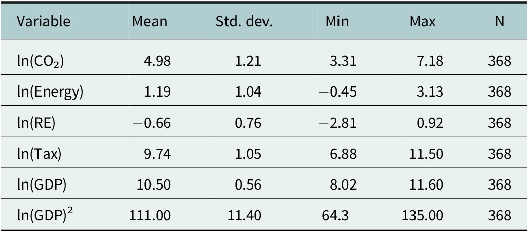
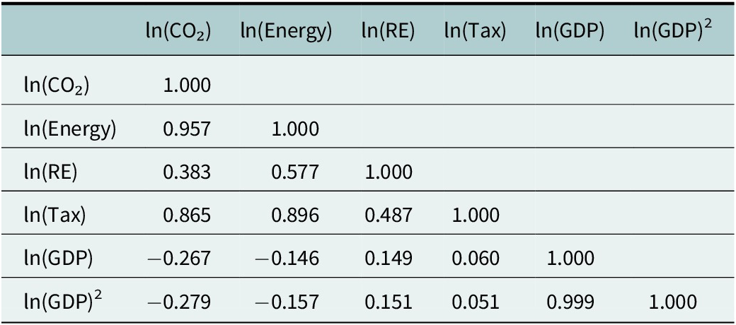
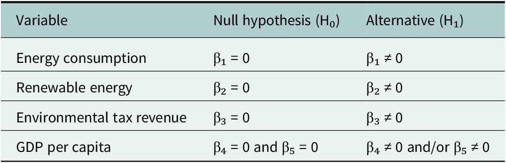


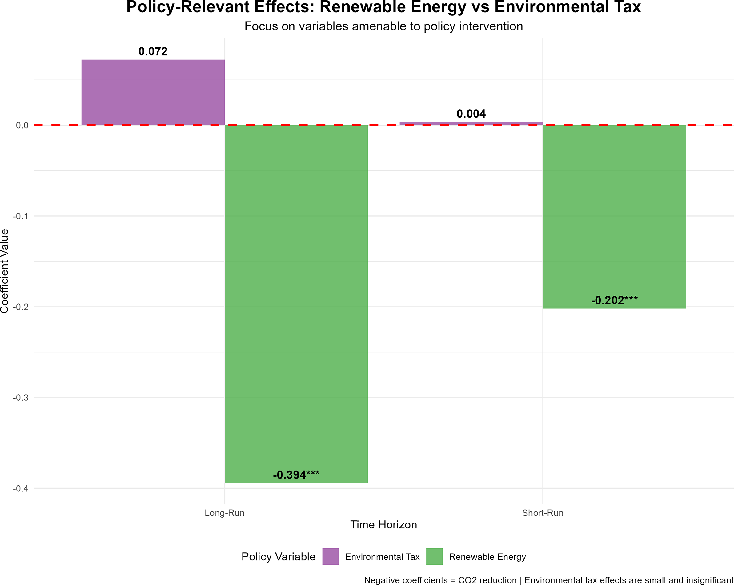


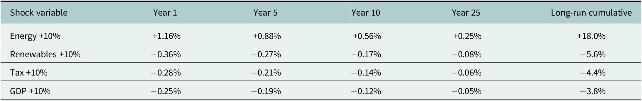


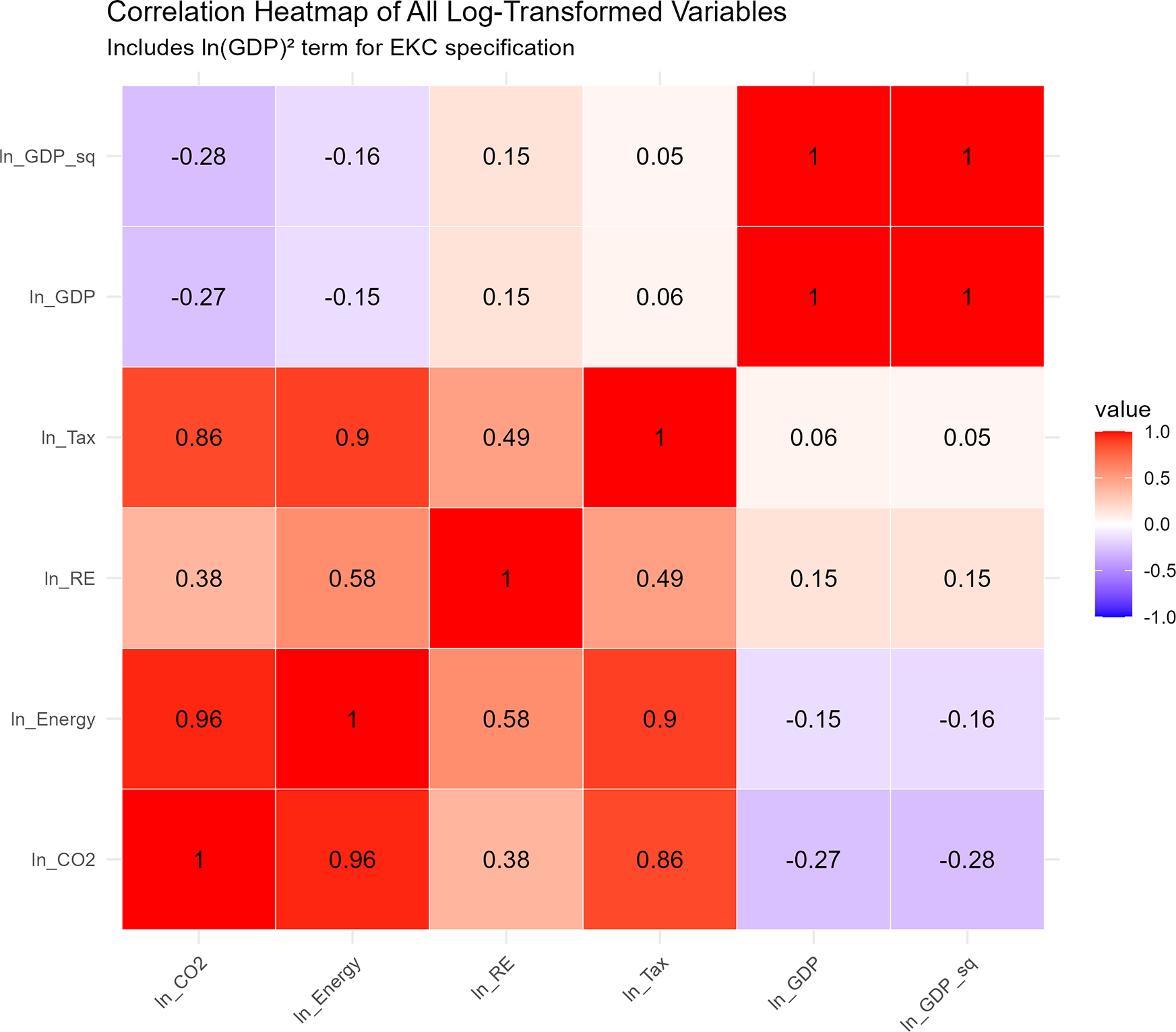

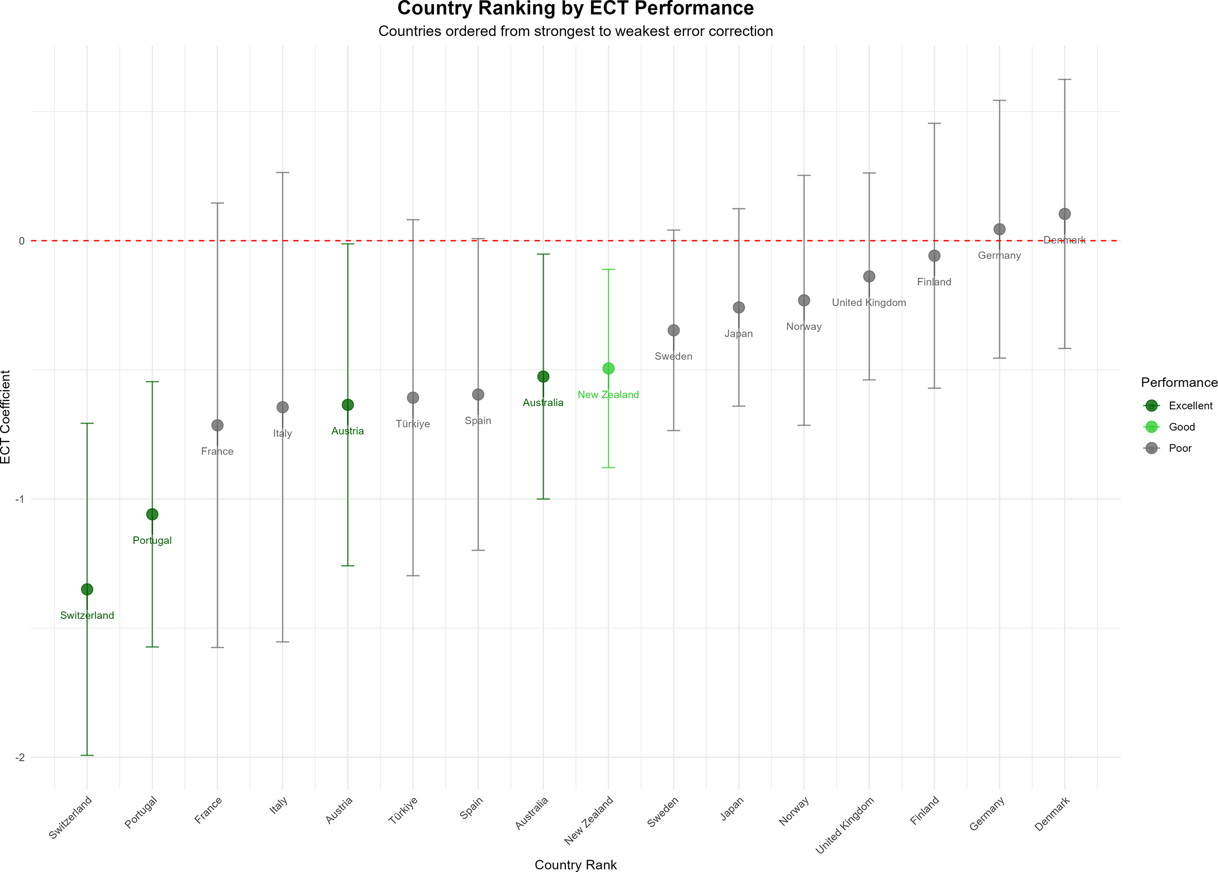


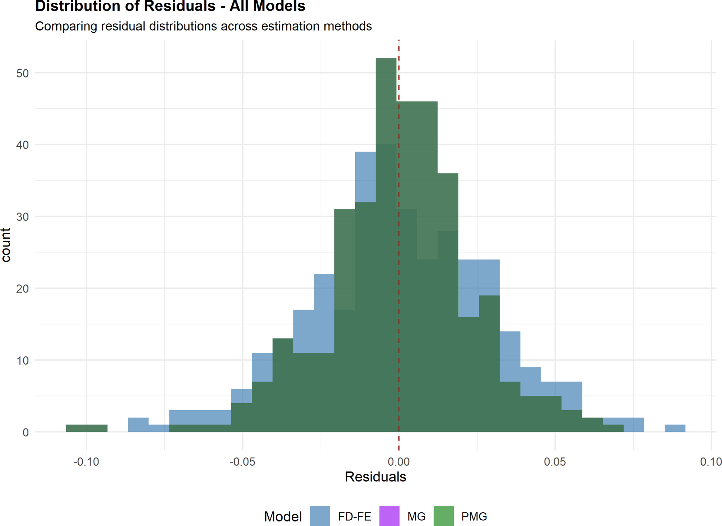
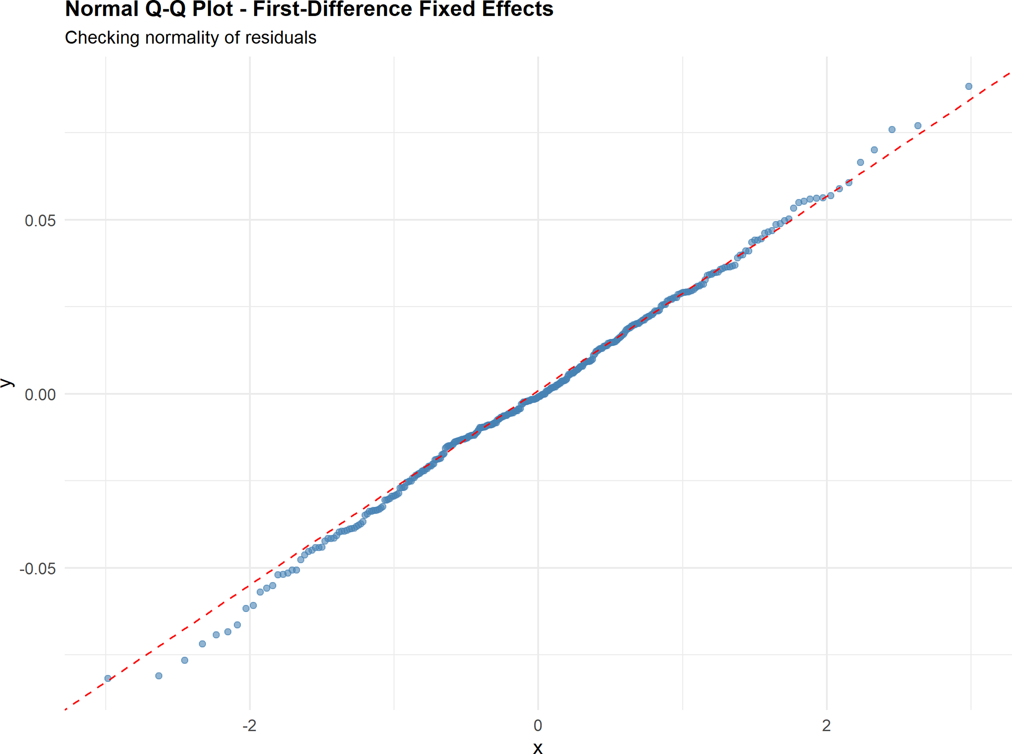
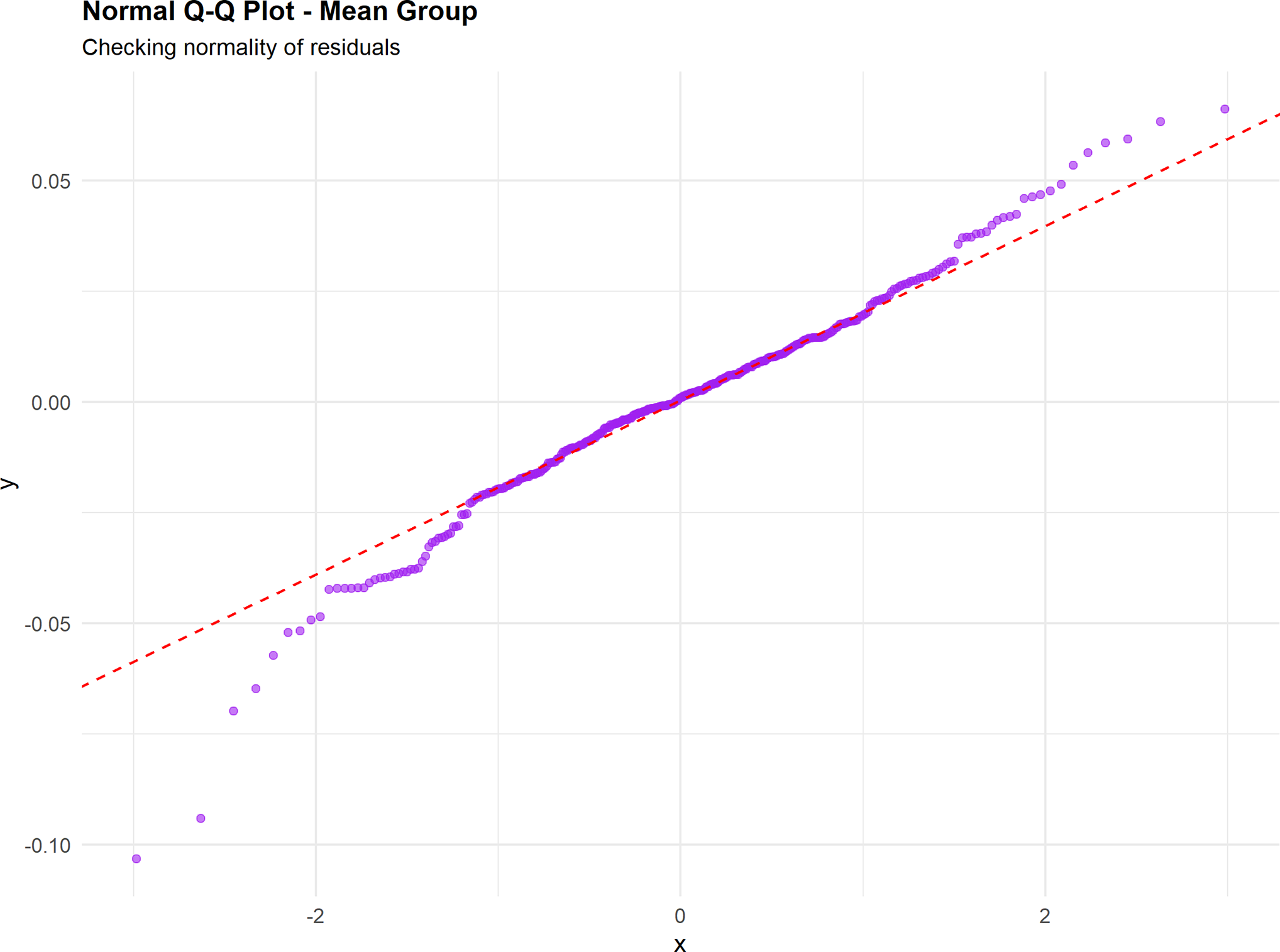
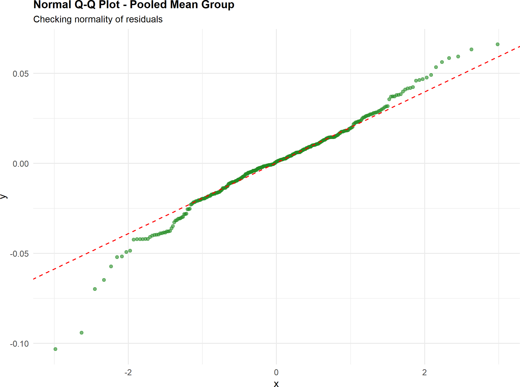

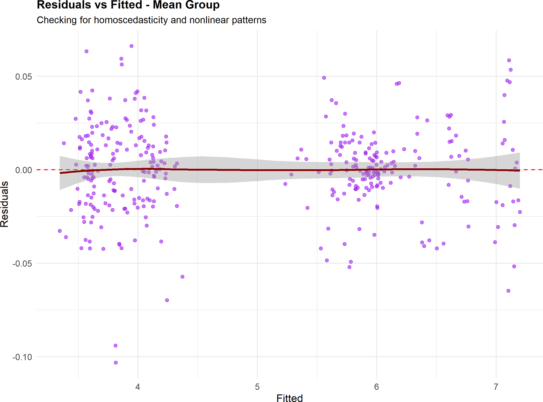


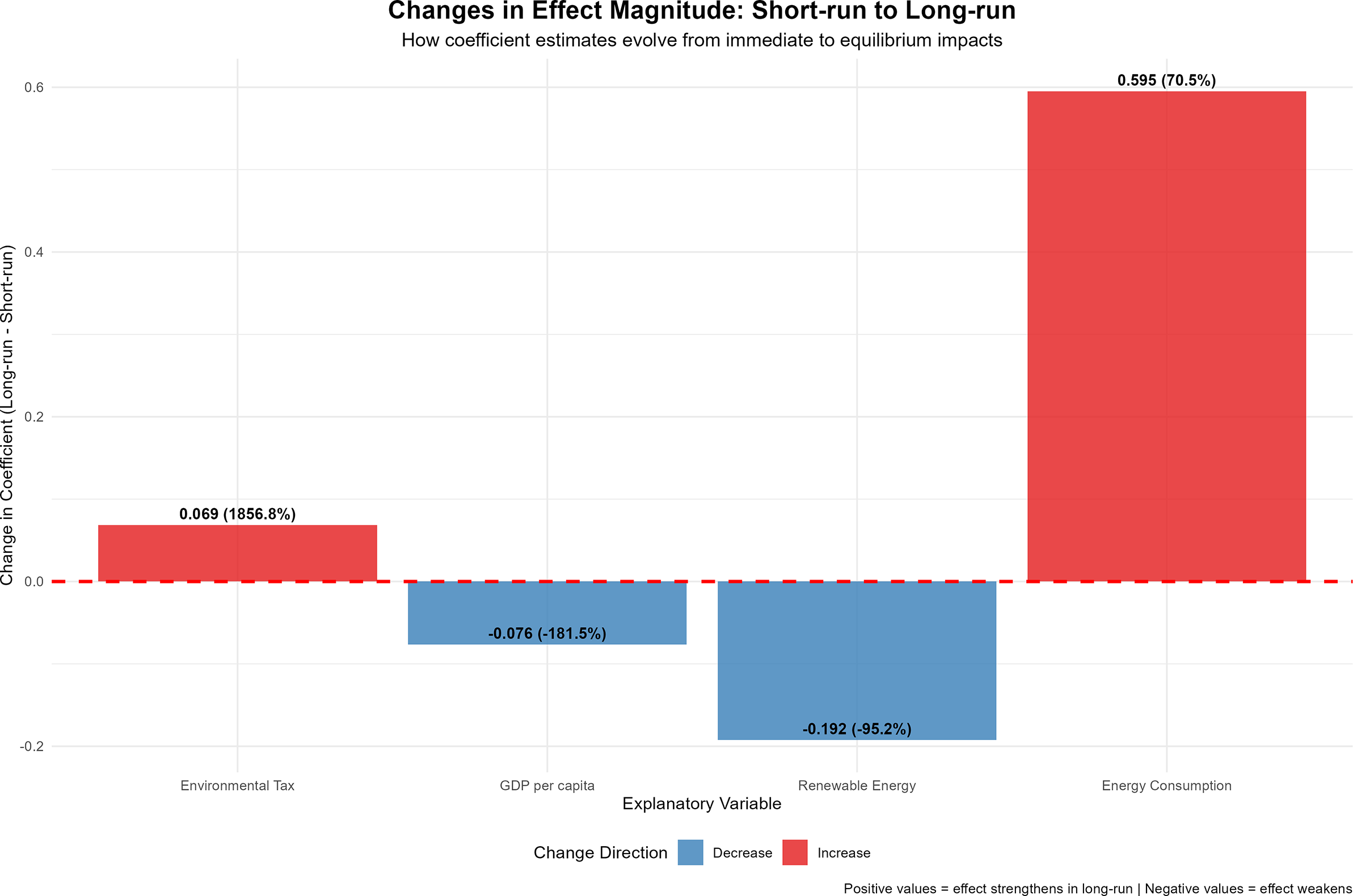


 Open access
Comments
Dear Editors,
I am pleased to submit our manuscript entitled “Assessing the Impact of Environmental Tax Revenue and Renewable Energy on Carbon Dioxide Emissions: A Panel Data Analysis” for consideration in Cambridge Prisms: Energy Transitions.
This paper examines how environmental tax revenue and renewable energy consumption jointly affect CO₂ emissions in seven advanced OECD countries—Australia, Denmark, France, Germany, Japan, Sweden, and the United Kingdom—over 2000–2022. Using panel data analysis with fixed and random effects models, we find that both higher environmental tax revenues and greater renewable energy use significantly reduce CO₂ emissions. Renewable energy is a particularly strong and consistent driver, while environmental taxes have a more modest but still meaningful effect. These results highlight the complementary roles of fiscal and clean energy policies in advancing decarbonization and sustainable growth.
The manuscript is original, has not been published elsewhere, and is not under review by any other journal.
Thank you for considering our submission.
Sincerely,
Rashad Baghirov (Corresponding Author)
Azerbaijan Tourism and Management University, Azerbaijan
Email: rashad.baghirov@hotmail.com
Co-authors:
Prof. Dr. Vusal Gasimli
Academy of Public Administration under the President of Azerbaijan,
Center for Analysis of Economic Reforms and Communication,
qasimlivusal@yahoo.com
Assoc. Prof. PhD Gunay Guliyeva
Center for Analysis of Economic Reforms and Communication,
Azerbaijan State University of Economics (UNEC), Business Management
ORCID ID: https://orcid.org/0000-0002-6782-0770
gunayguliyeva@unec.edu.az