


1. Introduction
The need to detect change accurately is a common problem for people in a wide range of domains, from business and politics to social relations and sports. In the academic literature, the canonical example is monitoring quality levels in a manufacturing process (Shewhart, Reference Shewhart1939, Girshick & Rubin, Reference Girshick and Rubin1952, Deming, Reference Deming1975), but recent research has broadened this paradigm beyond the field of operations research. Researchers in finance have invoked regime-shifts to explain documented patterns of under- and overreaction in asset pricing (Barberis et al., Reference Barberis, Shleifer and Vishny1998, Brav & Heaton, Reference Brav and Heaton2002, Gennaioli et al., Reference Gennaioli, Shleifer and Vishny2015), and economists have used change-point models to describe the challenges central bankers face in setting interest rates (Ball, Reference Ball1995, Blinder & Morgan, Reference Blinder and Morgan2005, Hamilton, Reference Hamilton, John and Uhlig2016, Brunnermeier et al., Reference Markus, Palia, Sastry and Sims2021). Even further afield, change detection is important to retailers assessing changes in consumer taste (Fader & Lattin, Reference Fader and Lattin1993), corporate strategists monitoring technological trends in their marketplace (Grove, Reference Grove1999), politicians tracking voter sentiment (Bowler & Donovan, Reference Bowler and Donovan1994), and individuals attending to their health (Steineck et al., Reference Steineck, Helgesen, Adolfsson, Dickman, Johansson, Johan Norlen and Holmberg2002) or their romantic partner’s commitment (Sprecher, Reference Sprecher1999). Finally and most recently, epidemiologists, policy makers, and the general population spent much of the COVID-19 pandemic figuring out whether a surge had peaked or a new COVID variant had taken hold (Atkeson et al., Reference Atkeson, Kopecky and Zha2021, Yang et al., Reference Yang, Han, Cui and Zhao2021). In all of these cases, “the states of the process are not directly observable but become gradually known with the sequential acquisition of fallible information over time” (Rapoport et al., Reference Rapoport, Burkheimer, Stein and Burkheimer1979). Indeed, the need to detect change accurately is ubiquitous, and it is therefore critical to understand the behavioral patterns involved in doing so.
These examples highlight the challenge of successfully identifying change: One must infer the true state or “regime” from unreliable signals, while balancing the costs of under-reacting (failing to realize change has occurred) against the costs of over-reacting (believing change has occurred when in fact it has not). For example, an investor needs to recognize when cyclical financial markets change from a “bear” to a “bull” market. Economic indicators are, at best, imprecise signals, with informativeness varying across indicators and over time. Under-reacting to signals of change means foregoing the chance to buy stocks at their lowest prices (or failing to sell a stock when it has peaked), whereas over-reacting entails acquiring shares that are still declining (or selling a stock too early when it would otherwise continue to rise).
A number of psychologists have investigated how successfully individuals navigate various experimental instantiations of change point detection tasks (i.e., Robinson, Reference Robinson1964, Chinnis & Peterson, Reference Chinnis and Peterson1968, Reference Chinnis and Peterson1970, Theios et al., Reference Theios, Brelsford and Ryan1971, Barry & Pitz, Reference Barry and Pitz1979, Rapoport et al., Reference Rapoport, Burkheimer, Stein and Burkheimer1979, Estes, Reference Estes1984, Brown & Steyvers, Reference Brown and Steyvers2009). A theme in this literature is that individuals respond to environmental conditions, but only partially. As Chinnis & Peterson Reference Chinnis and Peterson(1968) stated: “subjects, while sensitive to the difference in diagnostic value of the data in the two conditions, were not adequately sensitive” (p. 625). Massey & Wu Reference Massey and George(2005a) expanded on this theme, proposing the system-neglect hypothesis: People react primarily to the signals they observe and secondarily to the system that produced the signal. In their experiments, participants were exposed to signals generated by a number of different systems in which diagnosticity (i.e., the precision of the signal) and transition probability (i.e., the stability of the system) were varied. In our investor example, diagnosticity corresponds to the informativeness of the market indicators and transition probability corresponds to the historical rate of market vacillation. A diagnostic (vs. undiagnostic) signal might be an analyst report from a well-respected and historically successful (vs. unknown) securities analyst, or alternatively many disparate signals that largely point in the same direction (vs. a small number of disparate signals that are somewhat contradictory).Footnote 1 A stable (vs. unstable) system might be a more developed market such as the U.S. (vs. an emerging market such as Brazil).
Massey and Wu’s laboratory studies revealed a behavioral pattern consistent with system neglect: Under-reaction was most common in unstable systems with precise signals, whereas over-reaction was most prevalent in stable systems with noisy signals. Kremer et al. Reference Kremer, Moritz and Siemsen(2011) replicated and extended their work, finding evidence of system neglect in a time-series environment with continuous change and continuous signals. More recently, Seifert et al. Reference Seifert, Ulu and Guha2023 examined pricing decisions with impending regime shifts. They found a pattern similar to Massey and Wu in a rich setting in which there were buyers and sellers, a regime shift was either desirable or undesirable, and outcomes were either gains or losses (see also, Guha et al., Reference Guha, Seifert, Ulu, Federspiel, Montibeller and Seifert2024).Footnote 2
A common critique of behavioral decision research is that participants engage in relatively novel tasks in unfamiliar environments, without sufficient opportunity to learn (i.e., Coursey et al., Reference Coursey, Hovis and Schulze1987, Hertwig & Ortmann, Reference Hertwig and Ortmann2001, List, Reference List2003, Plott & Zeiler, Reference Plott and Zeiler2005, Erev & Haruvy, Reference Erev, Haruvy, John and Alvin2015). In Massey & Wu Reference Massey and George(2005a) (hereafter MW), for example, the diagnosticity and transition probability of the system changed after each of the 18 trials. On the one hand, this design enhanced the salience of the system variables, increasing the likelihood that participants would give them sufficient attention. On the other hand, this continuously changing design may have hindered participants’ ability to appropriately adjust to these dimensions by minimizing their opportunity to learn about a particular system and therefore raises questions about the robustness of the system-neglect hypothesis. Does the pattern of over- and under-reaction observed in MW persist in the face of the opportunity to learn? Or is the system-neglect phenomenon only observed in those inexperienced with the task and therefore less applicable to real-world settings where people have sufficient opportunities to learn? The present paper aims to fill these gaps in our understanding.
Although there is little doubt that experience can lead to learning, it is also well known that it does not always, especially for tasks involving probabilistic judgment (Brehmer, Reference Brehmer1980). Experimental studies in psychology and economics have found that experience can improve performance in probabilistic tasks such as conditional probability estimation (Martin & Gettys, Reference Martin and Gettys1969, Donnell & Du Charme, Reference Donnell and Du Charme1975), the Monty Hall Problem (Friedman, Reference Friedman1998), and the Newsvendor Problem (Bolton & Katok, Reference Bolton and Katok2008). However, learning is often limited and depends on the nature of the feedback (Martin & Gettys, Reference Martin and Gettys1969, Hogarth et al., Reference Hogarth, McKenzie, Gibbs and Marquis1991, Hogarth, Reference Hogarth2001). In particular, Hogarth et al. Reference Hogarth, McKenzie, Gibbs and Marquis(1991) found that the “exactingness” (i.e., the severity of penalties imposed for errors) of feedback had an inverted-U-shaped relationship with learning: while some penalty for errors helps, overly exacting feedback reduces learning. Importantly, this prior work has focused on static tasks in which the task parameters do not change over time; learning in dynamic tasks may be more limited since feedback across trials may not be relevant for future decisions (Schweitzer & Cachon, Reference Schweitzer and Cachon2000). While we expect feedback to be important for learning to detect change, what system characteristics give rise to consistent feedback with the right degree of exactingness?
The rest of the paper is organized as follows. We begin by describing the statistical process used in our experiment and reviewing the system-neglect hypothesis. Next, we present the experimental design, in which participants made probability judgments across 20 trials, each consisting of 10 periods, all in a single system that crossed three levels of diagnosticity (a measure of the informativeness of the signal) with four levels of transition probability (a measure of the stability of the environment). We discuss our results and examine how learning varies across conditions. We focus on two measures, earnings and reactions to signals of change. We then present a linear adjustment heuristic, which we term the δ-ϵ model, that provides good fits to both the normative standard of Bayesian updating, as well as the probabilities elicited from our participants. We use the δ-ϵ model to show that environments vary considerably in how exacting they are to deviations from the optimal δ-ϵ strategy, and in the consistency of feedback they provide how the earnings-maximizing δ and ϵ for one trial (a “local maxima”) performs on other trials. We show that a substantial portion of the differences in learning across environments can be explained by feedback consistency for that environment, as well as by “scope for learning” how close or far participants’ initial reactions (in the sense of δ and ϵ) are to optimal reactions. We conclude by discussing open questions and future directions.
2. Background and Theory
In this section, we introduce the design of our experiment and review the system-neglect hypothesis predictions for detecting changes in this statistical process.
2.1. Terminology
We begin by introducing key terms used throughout the paper. First, the system is the random process that generates binary signals (red or blue balls) in each of the 10 periods that make up a trial. Systems are dynamic in the sense that they can generate signals using two different sets of probability distributions, each of which we call a regime. A system is characterized by two system parameters: diagnosticity, or the informativeness of the signals it generates, and transition probability, or the likelihood of the system switching to the second regime.
2.2. Experimental Paradigm
Our experimental paradigm largely mirrors that of MW. Each trial t consists of 10 periods, with the system beginning in the red regime. There is, however, a transition probability q of switching to the blue regime before any period i (including the first period before any signal is drawn). If the system switches to the blue regime, it does not switch back. That is, the blue regime is an absorbing state.Footnote 3 The regime changes at  $\tau_t=1,...,11$, where $\tau_t=1$ indicates that the regime changes before the first signal is received and $\tau_t=11$ indicates that the regime did not shift during that trial.
The system generates either a red or blue signal in each period. A red signal is generated by the red regime with probability  $p_R \gt .5$ and by the blue regime with probability $p_B \lt .5$. Put differently, a red signal is more suggestive of a red regime, and a blue signal is more suggestive of a blue regime. The probabilities were symmetric in our experiment (i.e., $p_R=1-p_B$), so $p_R/p_B$ is a measure of the diagnosticity (d) of the signal, with larger diagnosticities corresponding to more precise and informative signals. Participants were given each of the relevant system parameters and told that their task was to guess which regime generated that period’s signal. More specifically, they estimated the probability that the system had switched to the blue regime. Importantly, at the end of each trial, participants received feedback about the true regime that governed each period of that trial.
Optimal responses to the task required application of Bayes’ Rule. Let  $B_i=1$ ( $B_i=0$) indicate that the stochastic process is in the blue (red) regime in period i, and let $b_i=1$ ( $b_i=0$) indicate that a blue (red) signal is observed in that period. If $H_i=(b_1,...,b_i)$ denotes the history of signals through period i, the Bayesian posterior odds of a change to the blue state after observing history Hi is:
 \begin{eqnarray}
\frac {p_i^b} {1-p_i^b} & = & \left( {\frac{{1 - (1 - q)^i }}{{(1 - q)^i }}}
\right)\sum\limits_{j = 1}^i {\frac{{q(1 - q)^{j - 1} }}{{1 - (1 -
q)^i }}d^{\left[ {i + 1 - j - \left( {2\sum\limits_{k = j}^i {b_k }
} \right)} \right]}, }
\end{eqnarray}
\begin{eqnarray}
\frac {p_i^b} {1-p_i^b} & = & \left( {\frac{{1 - (1 - q)^i }}{{(1 - q)^i }}}
\right)\sum\limits_{j = 1}^i {\frac{{q(1 - q)^{j - 1} }}{{1 - (1 -
q)^i }}d^{\left[ {i + 1 - j - \left( {2\sum\limits_{k = j}^i {b_k }
} \right)} \right]}, }
\end{eqnarray} where  $p_i^b=\Pr(B_i|H_i)$ denotes the Bayesian posterior probability that the process has switched to the blue regime by period i. The derivation for Eqn. (1) is found in Massey & Wu Reference Massey and George(2005b). Note also that the right hand side of Eqn. (1) factors out $(1-(1-q)^i))/(1-q)^i$, the “base rate” odds of a change to the blue regime in the absence of a signal.
Our experimental setting allowed us to compare individual judgments against the normative standard of Bayesian updating, as we provided participants with all the information necessary to calculate Bayesian responses and hence provide optimal judgments. Therefore, our experiment was designed to test the system-neglect hypothesis by investigating whether individuals update probability judgments as required by Bayesian updating and whether their ability to do so improves with experience.
2.3. The system-neglect hypothesis
The system-neglect hypothesis posits that people are more sensitive to signals than to system variables. This hypothesis extends work by Griffin & Tversky Reference Griffin and Tversky(1992), who proposed that people are disproportionately influenced by the strength of evidence (i.e., the effusiveness of a letter of recommendation) at the expense of its weight (i.e., the credibility of the letter writer) (see also, Benjamin, Reference Benjamin, Douglas Bernheim, DellaVigna and Laibson2019). This relative attention to strength over weight determines a person’s confidence, leading to a pattern of over-confidence when strength is high and weight is low, and under-confidence when strength is low but weight is high. For example, Griffin and Tversky, Reference Griffin and Tversky1992 investigated a static analog to our task in which participants judge whether a coin is biased heads or biased tails based on a sample of h heads out of n tosses. They found that judgments are more influenced by the sample proportion ( $h/n$), the strength of evidence, than the sample size (n), the weight of evidence. In another study, sample proportion again constituted the strength of evidence, with base rate serving as the weight of evidence in this instance.
In the context of our dynamic statistical process, we take the signal (i.e., the sequence of red and blue signals) to be the strength and the system parameters (i.e., the transition probability, q, and the diagnosticity, d) to be the weight. The critical implication of the system-neglect hypothesis is that individuals are more likely to over-react to signals of change in stable systems with noisy signals, and are more likely to under-react in unstable systems with precise signals. However, note that system neglect makes a relative prediction and is silent about overall levels of reaction; as such, it is consistent with patterns of only under-reaction or only over-reaction.
To provide a concrete example, consider four systems crossing two levels of diagnosticity, d = 1.5 and d = 9, with two transition probabilities, q = .05 and q = .20. Suppose that signals in the first two periods are both blue, i.e.,  $H_2=(1,1)$. The Bayesian posterior probabilities of a change to the blue regime are $\Pr(B_2|H_2)=.17$ when d = 1.5 and q = .05 (i.e., a noisy and stable system), but $\Pr(B_2|H_2)=.92$ when d = 9 and q = .20 (i.e., a precise and unstable system). If individuals give approximately the same response across all four conditions (for example, with a posterior probability of .60), they will over-react when d = 1.5 and q = .05 and under-react when d = 9 and q = .20. Of course, we do not expect participants to ignore the system parameters entirely. However, the system-neglect hypothesis requires that people attend too little to diagnosticity and transition probability and too much to the signals.
3. Learning Experiment
3.1. Participants, Stimuli, and Conditions
We recruited 240 students at a private Midwestern university as participants for a task advertised as a “probability estimation task.” Each participant was randomly assigned to one of the 12 experimental conditions, constructed by crossing three diagnosticity levels (d = 1.5, 3, and 9) with four transition probability levels (q = .02, .05, .10, and .20). These 12 systems were the same ones used in MW. The most important deviation from MW was switching to a between-participants design: Each participant only saw one set of system variables for all 20 trials.
Although we pre-generated the 20 random trials of 10 periods each using each condition’s system variables, participants received those 20 trials in randomized order. The actual series for each trial can be found in the Online Supplemental Materials (see A.1).Footnote 4
3.2. Compensation
We compensated participants according to a quadratic scoring rule that paid a maximum of $0.08 (i.e., if a participant indicated a 100% probability that the system was in the blue regime and it in fact was) and a minimum of -$0.08 (i.e., if a participant indicated a 100% probability that the system was in the blue regime but it was in fact still in the red regime). A quadratic scoring rule theoretically elicits true beliefs for a risk-neutral participant (, but see ). Although it was possible to lose money overall, doing so was extremely unlikely.Footnote 5 There was no fixed show-up fee.
3.3. Method
The experiment was conducted using a specially-designed Visual Basic program (see Section B in the Online Supplemental Materials for experiment screenshots). The program began by introducing the statistical process used in the experiment, explaining the system variables (pR, pB and q), how the computer would pick balls (i.e., the signals) from one of two bins (i.e., the regimes), and how the bin may switch. The program showed a schematic diagram of bin switching and then displayed four demonstration trials, each consisting of ten sequential draws. For these demonstration trials only, participants saw the actual sequence of bins that generated each signal, and therefore, if and when the process shifted from the red to the blue bin.
Participants were then told that, after seeing each ball, their task was to estimate the probability that the system had switched to the blue bin (i.e., the probability that the regime had shifted) by entering any number between 0 and 100. The computer then gave a detailed explanation of the incentive procedure including payment curves as a function of estimated probability and whether the bin had actually switched to the blue bin by that period. Participants completed two unpaid trials to better understand the interface and the incentive structure. After each trial, they were informed how much money they would have made or lost on that particular trial. At the end of each paid trial, participants received feedback about which bin generated each ball, earnings for that trial, and cumulative earnings in the experiment. Finally, participants completed 20 trials for actual pay.
4. Results
In this section, we summarize basic results for performance and learning. We look at earnings as a measure of performance. We report on Mean Absolute Difference (MAD) between empirical and Bayesian judgments in the Online Supplemental Materials, Section C.2. To test the system-neglect hypothesis, we then consider measures of reaction to indications of change as in MW.
In Section 5, we analyze the results through the lens of a heuristic model of δ-ϵ adjustment. This relatively simple “linear adjustment” model can mimic both Bayesian probabilities, as well as participants’ judgments. We also use this model to characterize the consistency of feedback within a system environment and show how this characterization relates to learning (or lack thereof) across conditions.
4.1. Earnings
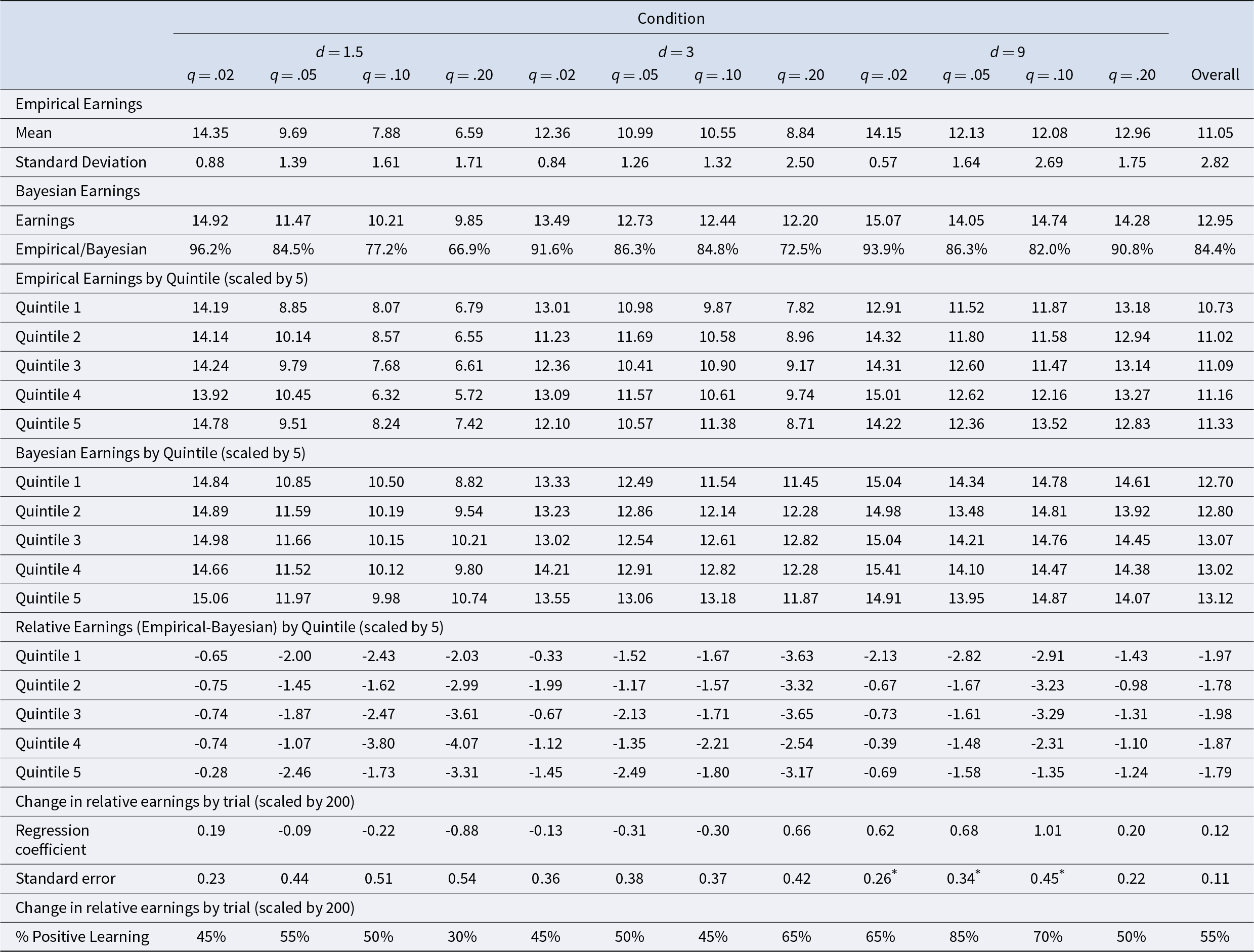
Recall that we paid participants based on the square of the difference between their subjective probability of having changed to the blue regime and the actual regime in that period (1 if blue, 0 if red). The mean absolute deviation (MAD) between their predictions and the actual regime was 0.150 (median = 0.073, sd = 0.192), generating mean total earnings of $11.05 over our 240 participants (range of $2.03 to $15.19 across participants) We define Bayesian earnings to be the earnings that would accrue if a participant’s probabilities were Bayesian as in Eqn. (1). Bayesian earnings were $12.95, while a participant who gave a probability of .5 for all 200 signals would have earned $8.00. Participants under-performed Bayesian earnings by a mean of $1.91 (range of $-0.27 to $12.34 across participants), earning 14.7% less than a Bayesian agent would earn. The rightmost column of Table 1 presents the mean empirical and Bayesian earnings overall for each condition.
Mean empirical and Bayesian earnings, and the difference between them, by condition and quintile (set of 4 trials). Also shown are linear regression coefficients of earnings as a function of trial, accounting for participant-level random intercepts and slopes, and the percentage of participants with improving earnings. Data by quintile and trial are re-scaled to facilitate comparison with overall earnings  $ ^*$ p < .05

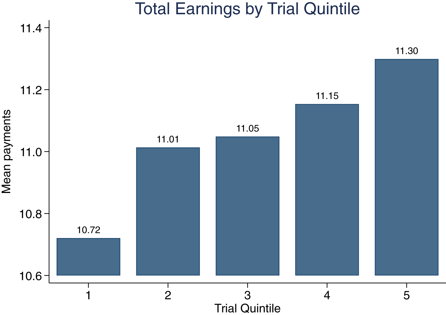
To investigate whether earnings increased over the course of 20 trials, we examined how earnings changed by trial quintile or quintile for short, where Quintile 1 consists of the first four trials experienced by a participant, etc. (results are virtually identical if we use quarters consisting of 5 trials). Table 1 lists the earnings by quintile, multiplied by five to be comparable to the overall earnings. Figure 1 shows that earnings increase monotonically over the quintiles, with earnings in Quintile 5 significantly larger than in Quintile 1 ( $ t = 2.38, p = 0.018 $). There was directional evidence of learning in 7 of the 12 conditions, but a significant increase in earnings only in the $ d = 3, q = .10$ ( $ t = 3.58, p = 0.002 $) condition.
Average total earnings by trial quintile, where Quintile 1 consists of the first four trials experienced by a participant, etc. Quintile earnings are normalized (multiplied by five) so that they are comparable to the total earnings over all 20 trials

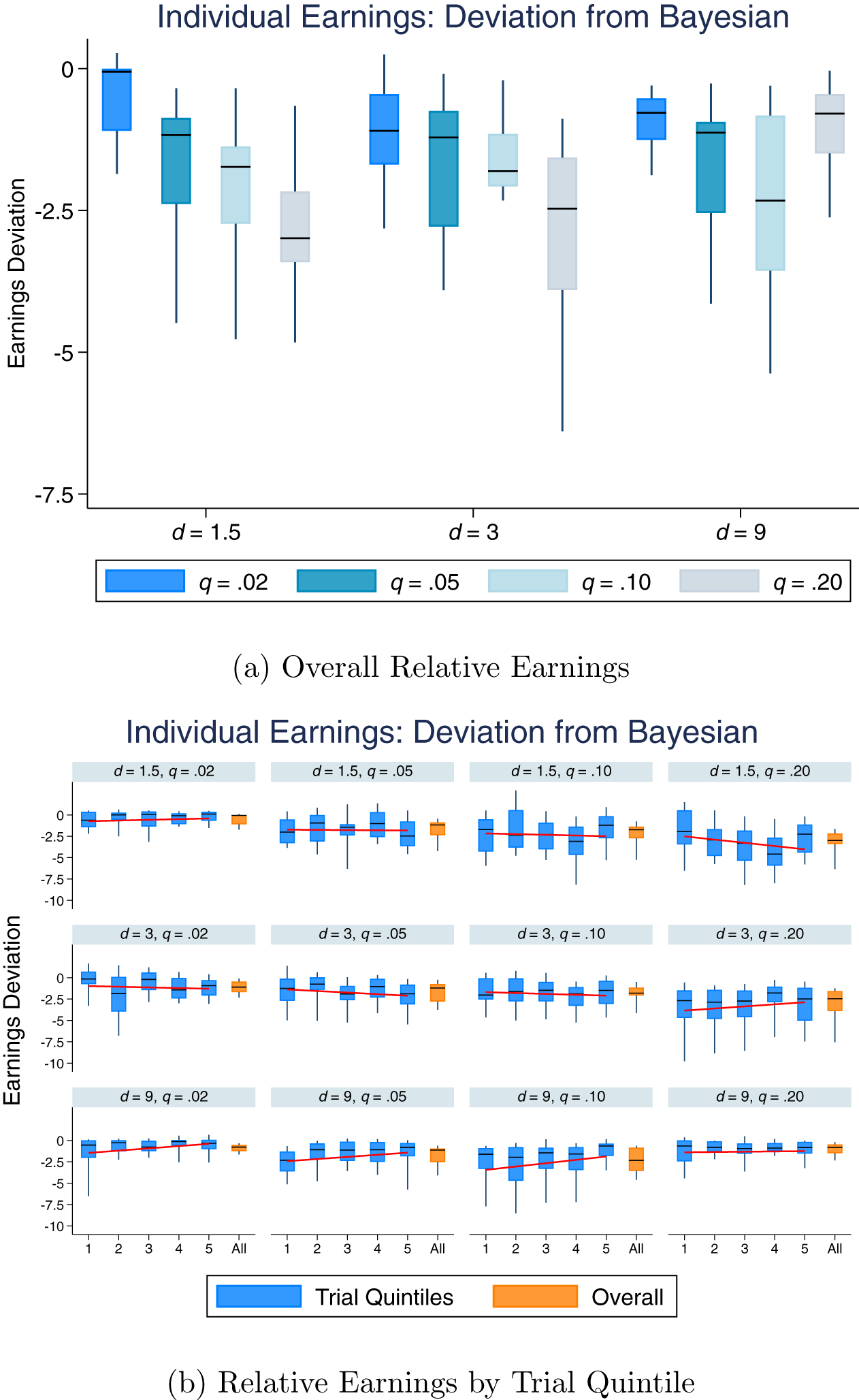
Since the random series are drawn from a noisy process—we also plot relative earnings—the difference between Bayesian earnings and empirical earnings—in Figure 2, (a) overall and (b) broken down by quintiles. Overall, relative earnings decreases with q, with the exception of the d = 9 condition. In addition, earnings are close to Bayesian for the  $d=1.5, q=.02$ and $d=9, q=.02$ conditions, and furthest from Bayesian for the $d=1.5,q=.20$ and $d=3,q=.20$ conditions. The plot of relative earnings by quintile again indicates that learning, if any, is modest and heterogeneous. Relative earnings increased directionally from Quintile 1 to Quintile 5 in 7 of the 12 conditions.
Relative earnings, by condition and trial quintile, with the box representing the inter-quartile range and the whiskers representing the range from 10 to 90 percentile of individuals. Relative earnings are the difference between empirical earnings and Bayesian earnings (i.e., what a Bayesian agent would earn). Panel (a) shows relative earnings aggregated over the 20 trials; Panel (b) shows the same measure for each of the five quintiles (blue), as well as overall (orange)

We conducted a statistical test of learning by running linear regressions of relative earnings on trial order for the 400 participant-trial observations per condition (20 participants per condition × 20 trials per participant), accounting for participant-level random intercepts and slopes. The coefficients on trial are found at the bottom of Table 1, with positive numbers corresponding to improving performance. Coefficients in 6 of the 12 conditions were positive and significant at the .05 level in the  $ d = 9, q = .02, .05, $ and .10 conditions. There was no evidence for learning overall ( $ z = 1.13, p = 0.46 $), We conducted the same analysis separately for each of the 240 participants, finding positive coefficients for 131 (55%) of the 240 participants overall (p = 0.175, two-tailed binomial test vs. 50%). The percentages of participants who had positive regression coefficients in each condition are shown at the bottom of Table 1.
In sum, we find modest evidence for learning in earnings and significant learning only in some of the high-diagnosticity conditions. Note, however, that earnings are a potentially noisy measure of performance, since the signals that participants receive can be unrepresentative of the underlying regimes that determine their earnings. Indeed, Bayesian judgments can produce lower earnings than non-Bayesian judgments for small, unrepresentative sequences. In C.2 in the Online Supplemental Materials, we show more pronounced, but still modest, learning for the Mean Absolute Deviation (MAD) between empirical and Bayesian probabilities.
4.2. Reactions
Whereas our analyses of earnings demonstrated modest learning that varied across conditions, the system-neglect hypothesis specifies how empirical probability judgments react to indications of change (i.e., blue signals) rather than their absolute levels. Therefore, to test for system neglect, we compared participants’ reactions (i.e., the change in probability judgments from period i − 1,  $p_{i-1}^e$, to period i, $p^e_i$, $\Delta p^e_i=p^e_i - p^e_{i-1}$) to the Bayesian reaction using the participant’s probability judgment in the previous period as the “prior.” That is, we constructed the Bayesian reaction by taking $p_{i-1}^e$ as the “prior” and applying Bayes’ Rule:
 \begin{equation}
\frac{{\bar{p}_i^b }}{{1 - \bar{p}_i^b }} = \frac{{{p}_{i-1}^e }}{{1 - {p}_{i-1}^e }} \left( {\frac{{1 }}{{1 - q }}} \right) \left( {\frac{{p_R }}{{p_B }}} \right)^{2b_i-1} + \left( {\frac{{q }}{{1 - q }}} \right) \left( {\frac{{p_R }}{{p_B }}} \right)^{2b_i-1}.
\end{equation}
\begin{equation}
\frac{{\bar{p}_i^b }}{{1 - \bar{p}_i^b }} = \frac{{{p}_{i-1}^e }}{{1 - {p}_{i-1}^e }} \left( {\frac{{1 }}{{1 - q }}} \right) \left( {\frac{{p_R }}{{p_B }}} \right)^{2b_i-1} + \left( {\frac{{q }}{{1 - q }}} \right) \left( {\frac{{p_R }}{{p_B }}} \right)^{2b_i-1}.
\end{equation} Importantly, this approach focuses only on reactions, granting participants their priors regardless of accuracy, and evaluating only how their judgments react to new information. We define errors in reaction as the difference between empirical and Bayesian reactions,  $p^e_i- \bar{p}^b_i$, with under-reaction indicating an empirical reaction that is less positive than the Bayesian reaction, $ p^e_i- \bar{p}^b_i \lt 0$, and over-reaction indicating the opposite, $ p^e_i- \bar{p}^b_i \gt 0$.
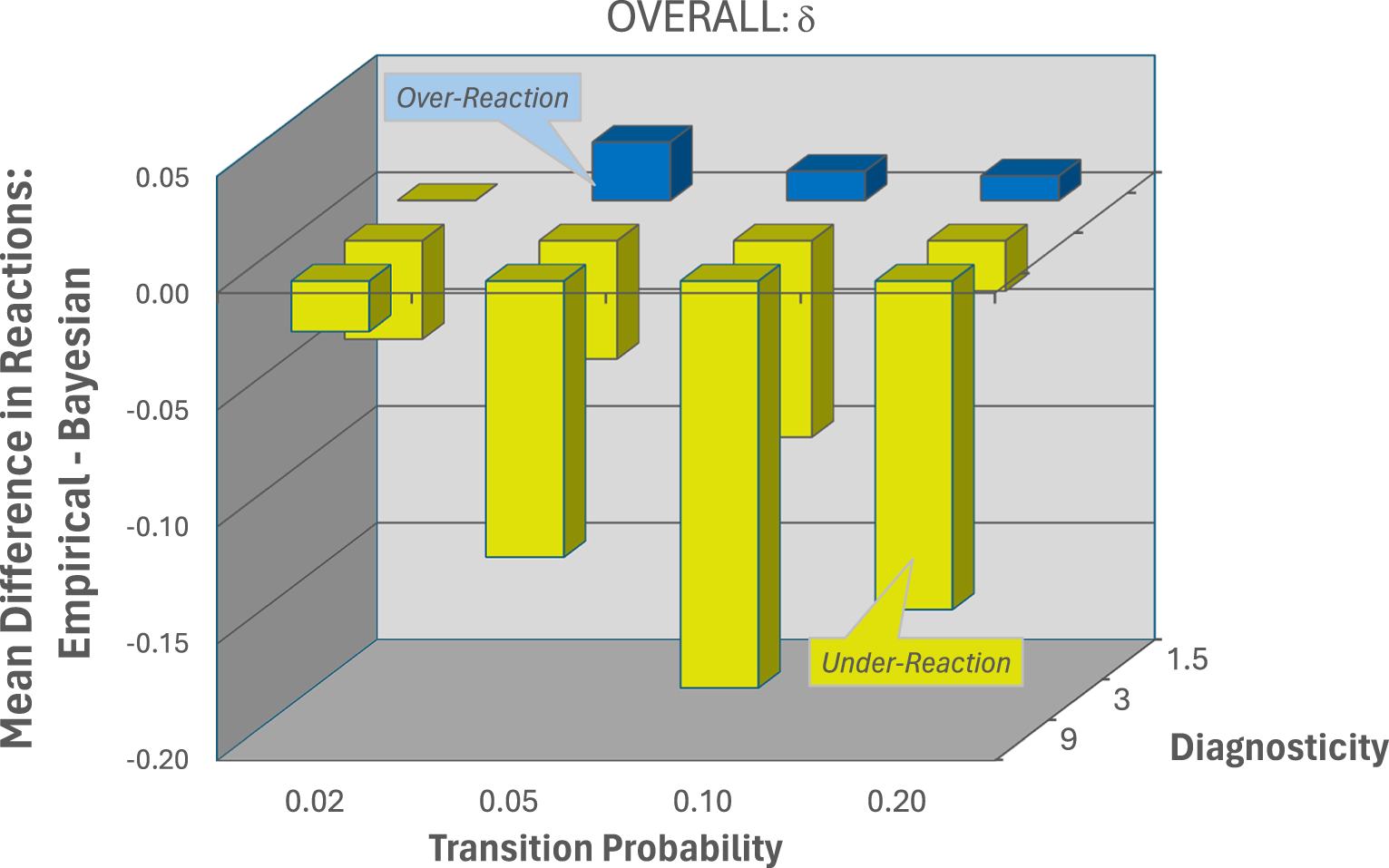
Figure 3 depicts the mean error in reactions to blue signals by condition (red signals are indicators of “non-change” and exhibit a different gradient; see Massey & Wu Reference Massey and George2005a). Recall that the system-neglect hypothesis predicts a greater tendency to under-react in more precise, less stable conditions, and to over-react in noisier, more stable conditions.
As predicted by the system-neglect hypothesis, and replicating MW, the greatest under-reaction occurred in the southeast-most cells (d = 9 with q = .05, q = .10, and q = .20, and d = 3 with q = .20), while the greatest over-reaction occurred in the northwest-most cells (d = 1.5 with q = .02 and q = .05 and d = 3 with q = .02). For 43 of the 48 pairwise comparisons between conditions, under-reaction increased monotonically with diagnosticity and transition probability (p < .001, two-tailed binomial test) (see Online Supplementary Materials, Table A15, for t-statistics for all 48 comparisons). For comparison, Figure 3 also plots the reactions from Massey & Wu Reference Massey and George(2005a). Note that the pattern of system neglect is somewhat more pronounced in that study compared to the current investigation.
Over- and under-reaction to blue signals, by condition, as measured by the mean difference between the empirical reactions and Bayesian reactions,  $ p^e_i- \bar{p}^b_i$. The panel (a) shows this measure for the current study. Panel (b) shows the same measure for Massey & Wu Reference Massey and George(2005a)

Figure 4 plots the same errors in reactions to blue signals by quintile. Note that the degree of system neglect is most pronounced in the first quintile but remains significant in the remaining four quintiles. For example, 40 of the 48 pairwise comparisons for the last quintile are still in the direction of the system-neglect hypothesis (p < .001, two-tailed binomial test). Figure 4 also suggests that the learning that does take place occurs mostly in the highly precise conditions (i.e., d = 9).
Over- and under-reaction, by condition and quintile (panels a-e), as measured by the mean difference between empirical reactions and Bayesian reactions,  $ p^e_i- \bar{p}^b_i$

In the Online Supplemental Materials, Section C.4, we follow MW in further analyzing the pattern of reactions in Figure 3 by estimating a “Quasi-Bayesian” model to test for learning to detect change. This model is in the spirit of Edwards Reference Edwards and Kleinmuntz(1968) and others, who compared empirical responsiveness to Bayesian responsiveness in “bookbag and poker chip” tasks. This analysis formally rules out the possibility that the hypothesized pattern is an artifact of the specific sequences of signals. This analysis corroborates Figure 4 that most of the learning that occurs corresponds to less conservative responses to highly diagnostic signals and when there is a high base-rate of change.
5. The δ-ϵ model of adjustment
Applying Bayes’ Rule to the change detection task is computationally complex and we do not expect participants to actually calculate Eqn. (1). In this section, we try to understand learning by viewing behavior through the lens of a computationally simpler and thus more psychologically plausible heuristic. First, we show that Bayes Rule for this task can be approximated with a simple linear adjustment heuristic, which we term the δ-ϵ model. The model adjusts the probability of a regime shift by δ with a signal indicative of change and by ϵ with a signal that is indicative of no change. We then demonstrate how the δ-ϵ model fits the empirical probabilities provided by our 240 participants. Finally, we show how the δ-ϵ model provides insight into which systems are less exacting for “non-optimal” behavior and which systems provide more consistent feedback.
5.1. The δ-ϵ model
Recall that a trial consists of 10 signals, bi,  $i=1,...,10$, where $b_{i}=1$ for a blue signal and $b_{i}=0$ for a red signal. Thus, the history of signals through i is given by $H_{i}=(b_{1},...,b_{i})$, with $B_{i}=1$ indicating that signal i was drawn from the blue bin.
Let pi indicate the probability that the ith signal was drawn from the Blue Bin, i.e., the probability that the regime has shifted by signal i,  $\Pr(B_{i}|H_{i})$. For now, pi refers to both normative (or, as we will show, approximately Bayesian) posterior probabilities, as well as empirical probabilities.
The δ-ϵ model is a linear adjustment model. We start with the first signal ( $i=1)$:
 \begin{align}
p_{1} = \left\{\begin{array}{lr}
q + \delta, & \text{if } b_{1}=1,\\
q + \epsilon, & \text{if } b_{1}=0.
\end{array}\right.
\end{align}
\begin{align}
p_{1} = \left\{\begin{array}{lr}
q + \delta, & \text{if } b_{1}=1,\\
q + \epsilon, & \text{if } b_{1}=0.
\end{array}\right.
\end{align} In the absence of a signal, the probability of a switch is taken to be q, the transition probability. The probability adjusts by δ with a signal consistent with change, and ϵ with a signal consistent with no change, where  $\delta \geq 0$ and ϵ may be positive or negative.
Adjustments for subsequent signals reflect the same linear adjustment, with an additional requirement that probabilities be bound between 0 and 1. In this model, the prior probability,  $p_{i-1}$ is a sufficient statistic for the history, $H_{i-1}$. We also investigated an alternative model in which blue signals “accumulate” (so that a red signal after many blue signals will not involve an adjustment), but we found that this model fits worse.
 \begin{align}
p_{i} = \left\{\begin{array}{lr}
\min(1,p_{i-1} + \delta), & \text{if } b_{i}=1,\\
\max(0,p_{i-1} + \epsilon), & \text{if } b_{i}=0.
\end{array}\right.
\end{align}
\begin{align}
p_{i} = \left\{\begin{array}{lr}
\min(1,p_{i-1} + \delta), & \text{if } b_{i}=1,\\
\max(0,p_{i-1} + \epsilon), & \text{if } b_{i}=0.
\end{array}\right.
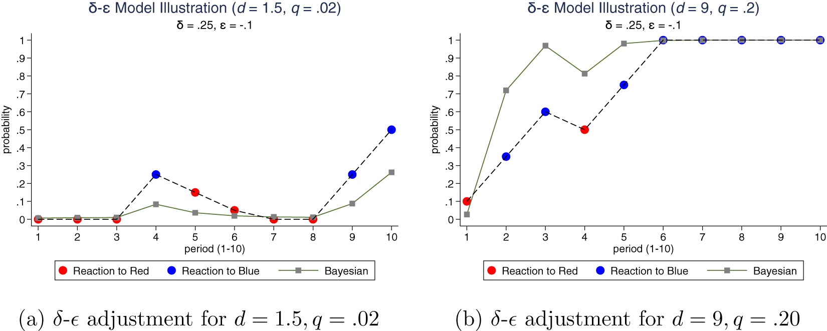
\end{align} We illustrate the model with two sequences from different systems, a system that generally produces under-reaction ( $d=9,q=.2$) and a system that generally produces over-reaction ( $d=1.5,q=.02$). Figure 5 illustrates how the model can produce system neglect. Here, we take δ = .25 and $\epsilon=-.10$ for both systems. In the noisy and stable system, reactions should be relatively muted, whereas in the informative and unstable system, reactions should be more pronounced. The same reactions in the two systems clearly produce the predicted pattern of system neglect, with probabilities too high when d = 1.5 and q = .02 and too low when d = 9 and q = .20.
Example of δ-ϵ adjustment that produces system neglect: over-reaction for (a) d = 1.5 and q = .02 and under-reaction for (b) d = 9 and q = .20, with δ = .25 and  $\epsilon=-.10$ for both systems

5.2. Correspondence to Bayesian probabilities
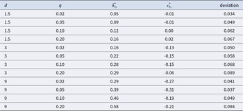
We next show that the δ-ϵ model can mimic Bayesian posteriors across all trials within a condition. To do so, we fit δb and ϵb to the Bayesian posteriors using a numerical grid search, in which we vary  $\delta_b \in [0,1]$ and $\epsilon_b \in [-1,.2]$ in increments of .01. The best-fitting parameters, $\delta_b^*$ and $\epsilon_b^*$, minimized the sum of squared deviations between the model probabilities and the Bayesian probabilities for the 20 trials in each condition. Estimates that included the practice trials are nearly identical. The best fitting parameters are found in Table 2. Note that as d increases, $\delta_b^*$ tends to get larger and $\epsilon_b^*$ tends to get smaller. Note also that the fits are reasonably good as indicated by the root mean squared error (RMSE) from Bayesian probabilities, with RMSEs ranging from 0.034 to 0.089 across the 12 conditions.
Fit of δ-ϵ model to Bayesian probabilities. The best fits minimize the sum of the squared deviations between the δ-ϵ and Bayesian probabilities, using a grid search. The deviation is the root mean squared error (RMSE) between the δ-ϵ and Bayesian probabilities
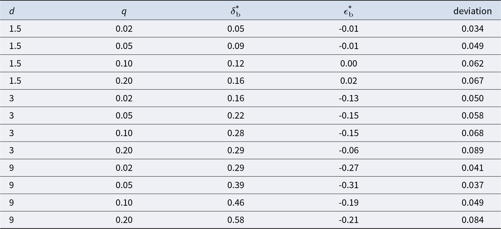
In Figure 5, we took δ = .25 and  $\epsilon=-.10$ for two different systems. Table 2 shows that $\delta_b^* = 0.05$ when d = 1.5 and q = .02, with $\delta_b^* = 0.58$ when d = 9 and q = .20. Thus, δ = .25 produces under-reaction in one system and over-reaction in the other system.Footnote 6
5.3. Correspondence to empirical probabilities
We next fit the δ-ϵ model to each of our 240 participants, using the grid search approach outlined in the previous section, denoting the fits to empirical probabilities, δe and ϵe. The model was fit individually to each participant’s 200 judgments for the 20 non-practice trials. For the most part, the model fits participants fairly well, with an average RMSE of 0.157 (range 0.000 to 0.410).
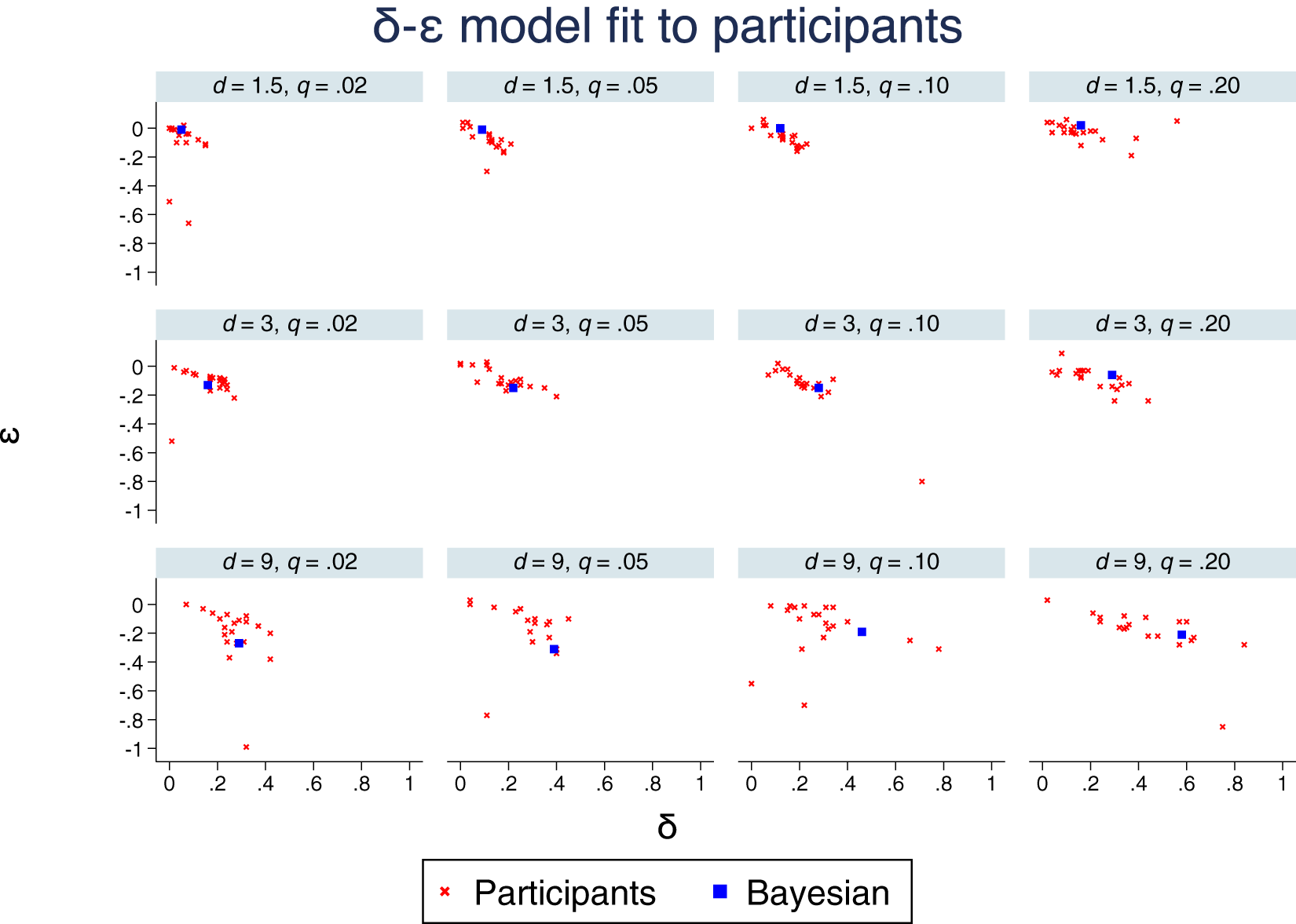
Figure 6 depicts a scatter plot of the estimates, δe and ϵe, along with the δb and ϵb for each condition. Note that this plot is consistent with system neglect. For d = 1.5 and q = .02, the δb and ϵb are northwest of most of the δe and ϵe fits, whereas the opposite holds for d = 9 and q = .20. We plot a measure of over- or under-reaction in Figure 7, the mean deviation between δb and δe. The pattern looks almost identical to that in Figure 3, with 43 of the relevant 48 pairwise comparisons consistent with system neglect (p < .001, two-tailed binomial test).
Estimates of δ-ϵ model fit to the 240 participants, by condition. The blue square shows the δ and ϵ for each condition that best fits Bayesian judgments

Over- and under-reaction to blue signals, by condition, as measured by the mean difference between the empirical and Bayesian δ,  $\delta_e-\delta_b$

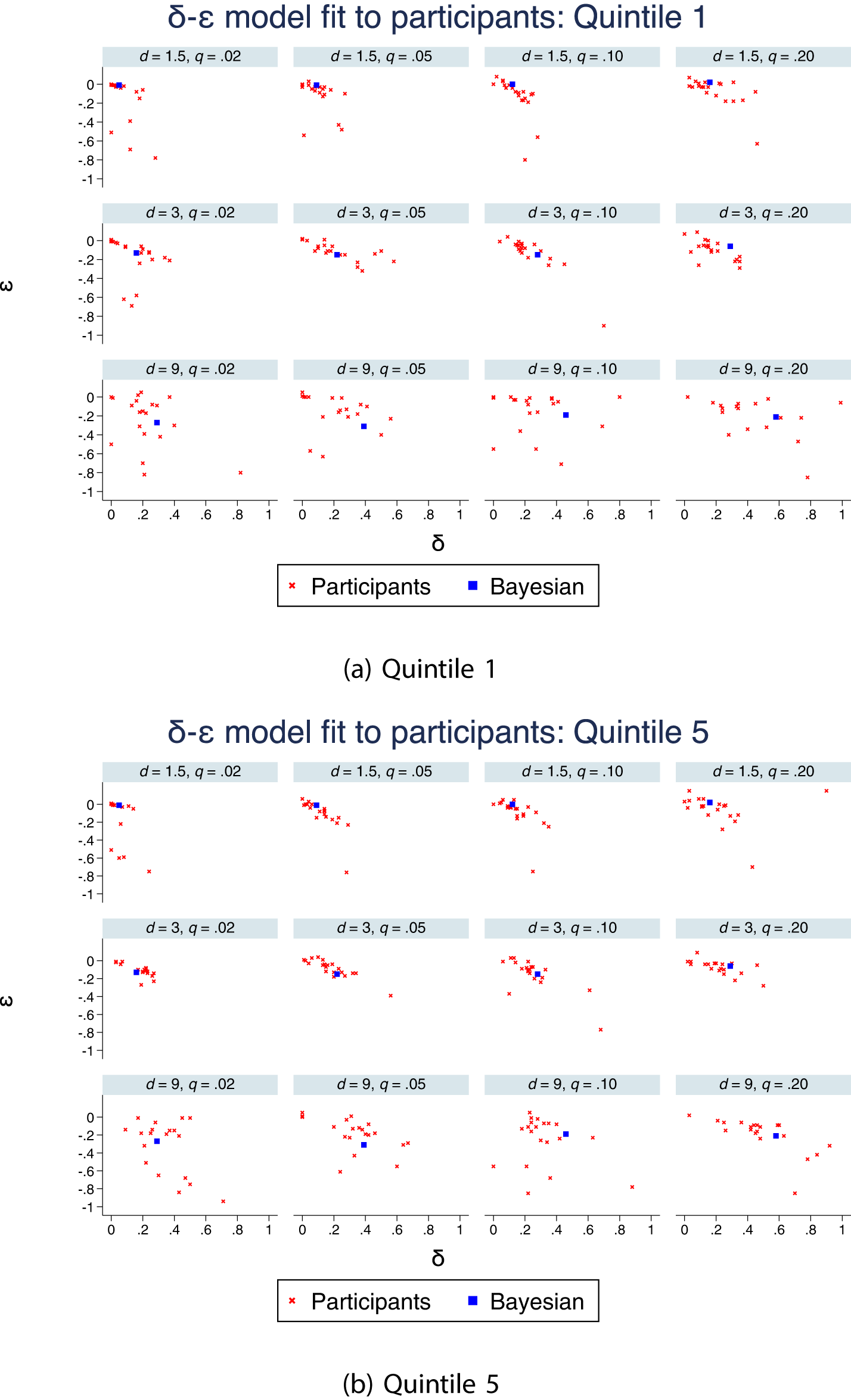
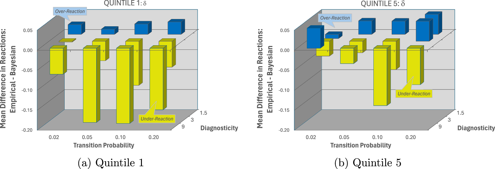
We also divide the data into quintiles and fit the model for each participant/quintile, δei and ϵei, where  $i=1,...5$. Figure 8 shows the estimates for Quintile 1 and Quintile 5. (Figure A.6 in the Online Supplemental Materials also depicts the other three quintiles.) We plot over- and under-reaction in δ, $\delta_b - \delta_{e}$ for Quintile 1 and Quintile 5 in Figure 9. Visually, it appears that under-reaction is less pronounced in Quintile 5, with much of the change happening in the d = 9 conditions, although over-reaction is slightly more pronounced. Indeed, 40 of the 48 relevant comparisons are in the predicted direction for Quintile 1, with 26 of the comparisons significant at the p < .05 level. In contrast, for Quintile 5, 38 of the 48 comparisons are consistent with system neglect, with only 19 significant at the p < .05 level.
Estimates of δ-ϵ model fit to the 240 participants, by condition and for the (a) first and (b) fifth quintile. Model is fit to 40 judgments per participant and quintile. The blue square shows the δ and ϵ for each condition that best fits Bayesian judgments

Over- and under-reaction to blue signals, by condition and for the (a) first and (b) fifth quintile, as measured by the mean difference between δe and δb, where δe is fit for each participant-quintile

5.4. Exactingness in the δ-ϵ framework
We have modeled reactions, both normative and empirical, in terms of linear adjustments to signals of change (δ) and signals of no change (ϵ). This δ-ϵ framework allows us to characterize each of our systems in terms of their conduciveness for learning.
We first examine how “exacting” earnings are to perturbations in δ and ϵ by looking at how earnings change when δ and ϵ parameters are non-optimal. For each condition, we calculate the overall earnings (i.e., total earnings for the 20 trials of the study) that would accrue by varying  $0 \leq \delta \leq 1$, and $-1 \leq \epsilon \leq 0.2$, in step sizes of .01. Let $\hat{\delta}$ and $\hat{\epsilon}$ denote the parameters that maximize total earnings for a condition. Let $E(\hat{\delta}, \hat{\epsilon})$, or $\hat{E}$ for simplicity, denote the total earnings for the earnings-maximizing set of parameters. For each condition, we compare earnings for combinations of parameter values, $E(\delta,\epsilon)$, to $\hat{E}$. We use a difference measure, $\hat{E}-E(\delta,\epsilon)$, as a measure of exactingness of earnings, but Figure A.9 in the Online Supplemental Materials depicts an alternative ratio measure, $E(\delta,\epsilon)/\hat{E}$, that provides nearly identical results. For example, for d = 1.5 and q = .02, earnings are maximized for $ \hat{\delta} = 0.06 $ and $ \hat{\epsilon} = -0.08 $, which produces a $ E(\hat{\delta},\hat{\epsilon}) = $15.03 $. By comparison, $ E(.3, -.2) = $10.78 $, for a difference of $4.25.
The contour plots in Figure 10 depict how exacting each system is to deviations from optimal levels of δ and ϵ. This analysis shows that systems vary considerably in exactingness. The systems with d = 1.5 (except for q = .02) are quite exacting in the sense that relatively small changes in reactions, δ or ϵ, can be costly in terms of performance. In comparison, the systems with d = 9, as well as d = 1.5, q = .02, are less exacting in the sense that relatively large changes in reactions lead to almost identical performance.
Contour Plots for Differences between Maximum and Implied Earnings,  $\hat{E}-E(\delta,\epsilon)$, for different combinations of δ and ϵ in each condition (panels a-l). The circle in the middle of the bright orange section references the earning maximizing combination of δ and ϵ, $\hat{\delta}$ and $\hat{\epsilon}$. The “B” captures the δ and ϵ that best fits Bayesian posteriors. The gray +’s represent the δ and ϵ that best fit the 20 participants in that condition (see Section 5.3)

5.5. Consistency of best responses
In our experiment, participants received explicit feedback after each trial about when the regime actually shifted and therefore what series of probability judgments would have maximized earnings for that trial. Although this feedback is unambiguous, it was only provided at the end of each trial and therefore was not entirely generalizable. That is, knowing the actual regimes for a past trial allows for a posteriori optimal responses for that trial but may not lead to learning how to provide a priori optimal responses for future trials unless this feedback is relatively consistent. We therefore explore the consistency of trial-level feedback by looking at how a “best response” for one trial performs on a different trial.
In our experiment, there are  $s=1,...,22$ series per condition.Footnote 7 For each series s, a participant saw a set of 10 signals, $H_{s}=(b_{1,s},...,b_{10,s})$. After the series was complete, participants were told if and when the regime changed. We denote that change as $\tau_s=1,...,11$, where $\tau_s=1$ indicates that the regime changes before the first signal was received and $\tau_s=11$ indicates that the regime did not shift during that series.
For each of the series,  $s=1,...,22$, within a condition, we determine the earnings for using a δ-ϵ response strategy, $E_s(\delta,\epsilon)$. Let $\hat{\delta}_s$ and $\hat{\epsilon}_s$ denote the “best response” strategy, i.e., the strategy that maximizes earnings given Hs and τs.Footnote 8 Our measure of consistency is $E_{s^{\prime}}(\hat{\delta}_{s},\hat{\epsilon}_{s})$, where $s,s^{\prime}=1,...,22$, which measures earnings for using the best response for series s for series s ʹ.
To illustrate, consider a series in the d = 9, q = .02 condition, where  $\tau_s=7$ and
  $H_s=(
1, 0, 0, 0, 0, 0, 1, 1, 0, 1)$. The best response to this series is
$H_s=(
1, 0, 0, 0, 0, 0, 1, 1, 0, 1)$. The best response to this series is  $ \hat{\delta}_s = 0.50 $ and $ \hat{\epsilon}_s = -0.27 $, with $ E_s(\hat{\delta}_s, \hat{\epsilon}_s) = \$ 0.75 $. Using $ \hat{\delta}_s $ and $ \hat{\epsilon}_s $ on other series s ʹ produces $ E_{s^{\prime}} (\hat{\delta}_{s},\hat{\epsilon}_{s}) $ that ranges from $0.48 to $0.80, with a mean of $0.76 and a standard deviation of $0.07. Therefore, the best response for Hs performs consistently well across other series in that condition.
By contrast,  $H_s=(0, 0, 1, 1, 1, 1, 1, 0, 1, 1)$ and $\tau_s=2$ for a series in the d = 3,q = .10 condition. The best response to this series is $\hat{\delta}_s = 0.38$ and $\hat{\epsilon}_s = 0.20$, yielding $ E_s(\hat{\delta}_s,\hat{\epsilon}_s) = \$ 0.22 $. In this case, the best response for s often does poorly for $ s^{\prime} \neq s $, with $ E_{s^{\prime}}(\hat{\delta}_{s},\hat{\epsilon}_{s})$ ranging from $-0.64 to $0.77, with a mean of $0.22 and a standard deviation of $0.59.
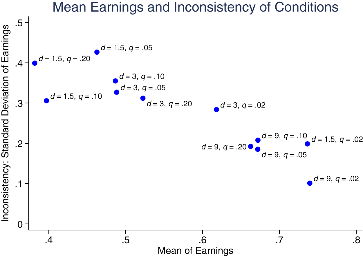
Figure 11 plots the mean and standard deviation of  $E_{s^{\prime}}(\hat{\delta}_{s},\hat{\epsilon}_{s})$ across the 12 conditions. Note that these two measures are strongly negatively correlated ( $ \rho = -0.89$). The conditions in which best responses for one series s also work for other series s ʹ (i.e., high consistency) also generate high earnings across all series. On the contrary, the conditions in which best responses for one series may not work for other series tend to produce lower earnings.
We should note that our consistency analysis naturally folds in the exactingness analysis from the previous section. Feedback is effectively inconsistent if the best response strategy for one series is very different than that for another series and earnings are exacting (i.e., punishing to deviations from best responses).
Mean and standard deviation of  $E_{s^{\prime}}(\hat{\delta}_{s},\hat{\epsilon}_{s})$ across the 12 conditions, where the standard deviation is our operationalization of (in)consistency

5.6. Using consistency to explain learning
The δ-ϵ framework allows us to characterize each of our systems in terms of their conduciveness for learning. We have modeled reactions, both Bayesian and empirical, in terms of linear adjustments to signals of change (δ) and signals of no change (ϵ).
In learning-friendly environments, the optimal adjustments in one situation are relatively similar to optimal adjustments in other situations. We hypothesize that this will affect learning. The more someone is reinforced for a particular behavior, the better off they are if that behavior is generally valuable. On the other hand, it will be difficult to learn when local optima tend to depart from global optima. Consider a golfer playing a course for the first time, trying to “figure out” the greens: how fast they are, how much break there is, etc. Some high-end courses maintain perfectly consistent conditions across all 18 greens, so what is learned on one green will apply to all greens. But that is rare. More often, there are some commonalities as well as some chance variations—closer mowing, dead patches, drainage challenges—that interfere with what a golfer can extrapolate across greens. We propose that, with change-point detection as with golf, the more consistent the rewards, the more conduciveness to learning.
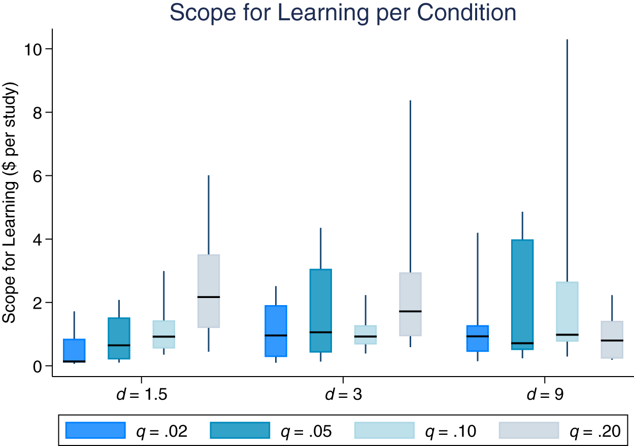
To evaluate the impact of consistency on learning, we relate changes in participant performance to the (in)consistency of their experimental condition, which we operationalize as the standard deviation of the consistency function,  $E_{s^{\prime}}(\hat{\delta}_{s},\hat{\epsilon}_{s})$. We operationalize learning as the difference in relative earnings (Bayesian minus empirical) between a participant’s first quintile (their first four paid trials) and their fifth quintile. In this analysis, we also consider each participant’s “scope for learning,” the difference between their first quintile earnings and the earnings that would be achieved by using the optimal δ and ϵ for their experimental condition. Scope for learning is important to control for as it is related to learning artifactually—i.e., those who start poorly in a noisy process are more likely to improve simply due to regression to the mean. Figure 12 shows that scope for learning varies across experimental conditions, revealing another form of system neglect—while optimal δ-ϵ parameters are quite different across experimental conditions, participants’ early behavior is relatively similar.
Box plot for scope for learning as measured by first quintile earnings relative to earnings that would be achieved by using the optimal δ and ϵ for their experimental condition. Scope for learning is rescaled to facilitate comparison with overall earnings for 20 trials. The box represents the interquartile range, with the whiskers representing the range from 10 to 90 percentile

We regress the difference in relative earnings between Quintile 1 to Quintile 5 on consistency, while controlling for scope for learning at the participant level. As predicted, learning is strongly related to consistency ( $ \beta = 6.71, SE = 2.03, t = -3.31, p = 0.001 $), with more learning occurring when consistency is high (i.e., low standard deviation of $ E_{s^{\prime}}(\hat{\delta}_{s},\hat{\epsilon}_{s})$) and poorer when consistency is low (i.e., high standard deviation of $ E_{s^{\prime}}(\hat{\delta}_{s},\hat{\epsilon}_{s})$). Learning was also positive related to scope for learning ( $ \beta = 0.25, SE = 0.09, t = 2.69, p = 0.008 $), with more learning when there was more scope for learning.
6. Discussion
Intuition suggests that the system-neglect pattern will attenuate with experience, with judgments becoming more Bayesian, but learning about probabilistic tasks is generally difficult (Brehmer, Reference Brehmer1980).
We examined learning across 12 conditions that varied in signal diagnosticity and system stability. Learning was more prevalent in highly diagnostic conditions. We also found that system neglect was partially attenuated by 20 trials of experience, especially for moderately and highly precise conditions, as well as for highly unstable conditions.
To better understand this variation in learning across conditions, we examined two characteristics of the learning environments, corresponding to the exactingness of deviations from optimal adjustments (in δ and ϵ terms) and the consistency of feedback. We found more learning in conditions with environments that provided consistent feedback (for our tasks, such environments are also more exacting). In other words, it is hard to learn when the best response for one series might perform poorly on the next series.
We should caution that our analysis is limited to only 12 conditions, with three levels of diagnosticity and four levels of transition probability, and only 20 sequences per condition.Footnote 9 However, we see the theoretical analysis used in Figure 11 as generative in that it can be readily used to investigate other incentive schemes and conditions.Footnote 10 Although we used a quadratic scoring system in our experimental setup, our consistency analysis can be extended to make predictions about different payment structures. In Section C.9.4 in the Online Supplemental Materials, we show that the basic pattern in Figure 11 holds for linear payoff schemes, as well as in a prediction task in which participants provide a binary prediction about the current regime (as in MW Study 3). However, a payment scheme in which participants are penalized by deviations from the normative Bayesian standard more or less equalizes the conditions: now, all conditions provide highly consistent feedback. Although there is perhaps no real world analog to a “deviation from Bayesian” payoff scheme, an experiment with such a payoff structure would provide a sharp test of our theoretical analysis.
It is also straightforward to extend our analysis to other systems with different combinations of d and q. In Section C.9.2 in the Online Supplemental Materials, we simulate a large number of systems with d ranging from 1.1 to 12.25 and q ranging from .005 to .52. Although mean and standard deviation of earnings are in general strongly negatively correlated as in Figure 11, this analysis identifies systems in which there is no correlation between mean and standard deviation. For the 12 systems used in our study, mean and standard deviation of  $E_{s^{\prime}}(\hat{\delta}_{s},\hat{\epsilon}_{s})$ are strongly negatively correlated. Indeed, the analysis we perform in Section 5.6, therefore, works as well with either measure as a covariate. We, however, have theorized that it is the consistency of feedback, as measured by standard deviation of $E_{s^{\prime}}(\hat{\delta}_{s},\hat{\epsilon}_{s})$, that either facilitates or inhibits learning. A study that used systems with no correlation between mean and standard deviation would unconfound these two measures and help to pinpoint the mechanism for what is driving learning.
Finally, our analysis of consistency is based on the idea that the best δ and ϵ response for one series may or not be effective on one other series. Friedman’s (Reference Friedman1998) analysis of the Monty Hall Problem suggests that individuals do not aggregate unless prompted. He found that prompting participants to track cumulative earnings for both strategies (the commonly chosen but not optimal strategy, “Stick”, as well as the optimal strategy, “Switch”) significantly increased the number of participants who switched (see also ).
Of course, in environments with low feedback consistency, aggregating over multiple series will yield more consistent feedback (see Online Supplemental Material, Section C.9.3). Counter-intuitively, reducing the frequency of feedback might foster aggregation, akin to providing feedback every few trials as in Lurie & Swaminathan Reference Lurie and Swaminathan(2009).
6.1. Implications
While our study focused on detecting regime shifts in a relatively abstract context, our findings have implications for understanding how managers and policy-makers can improve their decisions in dynamic real-world contexts, such as pricing (Seifert et al., Reference Seifert, Ulu and Guha2023) and stocking (Kremer et al., Reference Kremer, Moritz and Siemsen2011). Depending on the decision environment, decision makers might under-react to early signs of system change, leading to delayed responses and potential losses. Conversely, they might over-react to minor fluctuations in performance metrics, resulting in unnecessary strategic shifts. Future research should examine whether decision makers improve their decision making with experience in such contexts, whether in laboratory simulations or with real-world data.
The influence of environmental factors on learning has direct implications for decision makers. Obviously, it would be helpful to increase the quality or quantity of feedback available to a decision maker. For example, instituting a waiting period before reacting to signals of change could help reduce feedback inconsistency and therefore rates of reacting to a false alarm. Unfortunately, firms often do not or cannot control the feedback available in their environment. However, they may be able to improve decision-makers’ attention to feedback, by enhanced record-keeping or through activities explicitly aimed at learning from the past (Cyert & March, Reference Cyert and March1963, Friedman, Reference Friedman1998). Another approach is the use of policies to restrict decision-makers’ freedom (Heath et al., Reference Heath, Larrick, Klayman, Staw and Cummings1998) with the goal of avoiding “noise chasing” (i.e., over-reacting to inconsistent feedback). Both of these approaches—learning programs and policy-based decisions—are ways to improve institutional memory, an adaptive response to environments with inconsistent feedback. We should also note that although feedback in some conditions in our study was inconsistent, feedback was at least immediate, clear, and vivid, all qualities that facilitate learning (Nisbett & Ross, Reference Nisbett and Ross1980, Hogarth, Reference Hogarth2001, Maddox et al., Reference Maddox, Gregory Ashby and Bohil2003). Naturally occurring feedback, in contrast, is likely to be delayed, ambiguous, and obscure.
7. Conclusion
Our paper establishes the robustness of system neglect in people’s change-point detection and demonstrates the relationship between characteristics of an environment and learning. In the end, we are somewhat sober about the ability of individuals to avoid systematic over- and under-reaction in non-stationary environments. However, we are also encouraged by the possibility of learning. Together these sentiments suggest that an important directions for future research is to understand how different decision environments impact the potential for learning to detect change.
Supplementary material
The supplementary material for this article can be found at https://doi.org/.10.1017/eec.2024.9.
Replication packages
All experiment materials, data, and statistical code have been posted at: https://osf.io/5vy9m.
Acknowledgements
It is extremely important since it’s for a special issue dedicated to my deceased colleague. This paper is dedicated to Amnon Rapoport, whose papers (Rapoport and Burkheimer, Reference Wang, George and Shih-Wei1973; Stein and Rapoport, Reference Stein and Rapoport1978) and book (Rapoport et al., Reference Rapoport, Burkheimer, Stein and Burkheimer1979) on this topic and broader work on dynamic decision making inspired the last two authors when they first started thinking about change point detection. The first author deeply misses Amnon, cherishing the memories of him as both a colleague and a friend. We also thank the guest editor, David Budescu, and the reviewers for their useful comments.


 Open access