NOMENCLATURE
- S +22
transverse tensile strength, MPa
- E 22
transverse stiffness, MPa
- Vf
fiber volume fraction
- φ
degree of cure $\text{d}\phi /\text{d}t$
rate of cure, s−1
- t
time, s
- T
temperature, K
- H
heat of reaction, J/tonne
- Hr
total heat of reaction, J/tonne
- M
plane wave modulus, MPa
- ΔE 1, ΔE 2
activation energies, J
- f
cure kinetics function
- A 1, A 2
frequency-type rate equation parameters, s−1
- ρ
mass density, tonne/mm3
- cp
specific heat capacity, mJ/tonne-K
- κ
thermal conductivity, mW/mm-K
- δij
Kronecker delta
- σ
stress, MPa
- ε
strain
- εc
cure shrinkage strain
- α
thermal expansion coefficient, mm/mm-K
- E
Young’s modulus, MPa
- ν
Poisson’s ratio
- M
per-network plane wave modulus, MPa
- K
per-network bulk modulus, MPa
- μ
per-network shear modulus, MPa
- Mexp
global plane wave modulus, MPa
- μexp
global shear modulus, MPa
- GIC
mode I fracture toughness, N/mm
- gIC
normalised mode I fracture toughness, N/mm2
- h
characteristic element length, mm
- σcr
critical mode I fracture stress, MPa
- D
stiffness reduction factor due to softening
- σp
maximum principal stress, MPa
- εp
maximum principal strain
- εf
ultimate tensile fracture strain
- Ef 11
axial fibre modulus
- Ef 22
transverse fibre modulus
- νf12
fiber Poisson’s ratio in 1-2 plane
- Gf 12
fiber shear modulus in 1-2 plane
- Gf 23
fiber shear modulus in 2-3 plane
- Vf
fiber volume fraction in the tow
- σtow, +cr
tow tensile failure stress (axial)
- G tow, +IC
mode I tow fracture toughness (axial)

1.0 INTRODUCTION
The future of aircraft and spacecraft production will be dominated by automation in conjunction with advanced lightweight materials that afford life-cycle cost reductions(Reference Beukers, van Tooren and Vermeeren1). Using mass-produced textile fibre preforms in conjunction with innovative tooling and resin transfer molding processes will lead to better performing vehicles that have longer fatigue lives and no corrosion problems. This trend will continue to evolve leading to air vehicles that are made with cost-effective textile fibre composites and 3D printed structures that incorporate multi-materials. With stringent demands placed on certifying the structure of an aircraft, the development and use of robust, high-fidelity computational models for structural analysis will become paramount for cost savings. Indeed, the field of Integrated Computational Materials Engineering (ICME) has emerged as a beehive of activity(Reference Davies2-Reference Allison5). Within ICME, it is increasingly recognised that the manufacturing process influences the microstructure of a material, which in turn dictates performance.
Future certification and insertion of multi-material structures will be accelerated through the development of better computational models for analysis. This requires a thorough understanding of each stage of the production cycle. Mechanics- and thermodynamics-based models that incorporate the correct (experimentally observed) physics at each stage will emerge as the method of choice for ICME methodologies to be used in certification of future lightweight composite aerostructures. The need for physics-based damage, failure, and durability analysis models(Reference Pineda, Waas and Bednarcyk6) that can accurately capture the experimentally observed mechanical performance of air vehicle structures and structural components, has been identified as the most pressing industry need today in support of accelerating the development of high-performing materials for insertion in air vehicles. An urgent call to rise up to this challenge was evident in the keynote lectures presented recently at the 2015 American Society of Composites Meeting(Reference Talreja7).
ICME and its needs as it applies to materials in general are amply covered in the papers by Arnold et al(Reference Arnold, Cebon and Ashby8,Reference Arnold, Holland, Bednarcyk and Pineda9) . Here we focus on an important stage of the ICME process, that of understanding the effects of the curing process on the subsequent state and mechanical response of Fibre-Reinforced Polymer Matrix Composites (FRPCs). Since FRPCs contain a polymer matrix that surrounds the interspersed fibres, good understanding of the matrix state during the curing process is necessary to have sufficient control over the quality of the cured product. The state of the matrix during curing can be altered by the presence of fibres and their coatings, and also by details of the curing cycle. The curing matrix undergoes shrinkage due to chemical processes, reactions with the fibre surfaces, and heat release during chemical reactions, all of which gives rise to internal stress generation. Plepys and Farris(Reference Plepys and Farris10) and Plepys et al(Reference Plepys, Vratsanos and Farris11) employed Finite Element (FE) calculations using incremental elasticity to show tensile residual stress buildup of up to 28MPa post cure in a three-dimensionally constrained Epon 828 epoxy resin. Merzlyakov et al(Reference Merzlyakov, McKenna and Simon12) quantified the variation of tensile stresses during cure and subsequent thermal cycling. Chekanov et al(Reference Chekanov, Korotkov, Rozenberg, Dhzavadyan and Bogdanova13) have reported various types of defects that may form in a constrained epoxy resin system undergoing curing. Rabearison et al(Reference Rabearison, Jochum and Grandidier14) studied the curing of a thick epoxy tube using a FE model and concluded that high-stress gradients developed during differential curing can cause cracking. Song and Waas(Reference Song, Waas, Shahwan, Xiao and Faruque15) have shown that the use of bulk matrix properties (cured without fibres) in numerical predictions of compression response of a 2D triaxially braided composite Representative Volume Element (RVE) can lead to erroneous results – the computed compressive strength being noticeably higher than the experimentally measured strength. They observed that the tow compressive kinking failure mode, which controls compressive strength, was found to be sensitive to the nonlinear shear response of the matrix and initial fibre misalignment. It has been previously recognised that cure shrinkage in the matrix can influence the final shape of a composite structure(Reference Kim and Hahn16).
Depending on the constituent chemistry of the matrix and the fibre surfaces, the thermal cycle prescribed, and the fracture and strength properties of a curing matrix and fibres (these change with temperature) during the transition from a gel state to a solid state, a fibre-reinforced composite can and may undergo damage and cracking during the cure cycle. It has been observed that these cracks usually lie within the matrix, but, here again, the internal stresses and the resistance to fracture of the matrix and the fibre/matrix interface, all of which are a function of the temperature, will govern where that fracture will occur. Therefore, the state of the matrix within a cured FRPC structure exhibits in situ matrix properties, which are effective properties of the matrix that take into account unintended imperfections caused in the matrix due to the cure process, including the presence of residual stresses. That is, the in situ matrix properties, where the matrix is treated as a ‘new’ material with a reference configuration that corresponds to the post-cured state, deviate from idealised or ‘virgin’ matrix properties of the bulk matrix. The in situ matrix properties can be extracted from an inverse analysis through the uniaxial tensile response of a ± 45° laminate, and this is convenient in engineering analysis of cured composites(Reference Ng, Salvi and Waas17).
For ICME to be successful, it is necessary to have good knowledge of the influence of the cure cycle on the subsequent mechanical response of a FRPC structure, be it a pre-preg-type straight fibre laminate or a textile fibre fabric that reinforces a matrix. For a particular fibre-matrix laminate system, the optimal cure cycle can be identified such that the cured product has the desired strength and stiffness. Efforts to optimise various aspects of the cure cycle for mitigating the residual stresses generated during cure can be found in the studies of Li et al(Reference Li, Zhu, Geubelle and Tucker18), Gopal et al(Reference Gopal, Adali and Verijenko19) and White and Hahn(Reference White and Hahn20).
ICME of FRPCs also encompasses other aspects of post-cure response. These include cohesive zone modelling(Reference Sills and Thouless21-Reference Gustafson and Waas24), modelling notched strength(Reference Pineda, Waas and Bednarcyk6,Reference Wisnom, Hallett and Soutis25-Reference Davidson, Pineda, Heinrich and Waas29) , compressive failure(Reference Prabhakar and Waas30,Reference Heinrich, Alridge, Wineman, Kieffer, Waas and Shahwan31) , flexural response of textiles(Reference Zhang, Waas and Yen32,Reference Zhang, Waas and Yen33) , and transverse cracking(Reference Singh and Talreja34). In addition, several micromechanics-based models provide insights on capturing experimental observations and providing mechanical properties that can be used for up-scaling in structural level calculations(Reference Pineda, Bednarcyk, Waas and Arnold28,Reference Aboudi35-Reference Prabhakar and Waas38) . While several other papers address various aspects of ICME of FRPCs and ceramic matrix composites(Reference Meyer and Waas39), this paper focuses on the specific topic of cure-induced effects on subsequent mechanical response of FRPCs.
The effects of the cure cycle on possible damage accumulation during cure and subsequent in-service performance at the microstructural level are studied by using randomly packed RVEs having a total of 20 fibres. These are representative of a typical straight fibre ply material or a textile fibre tow. A plain weave textile composite RVE is also studied to illustrate the effects of curing on tensile strength of a textile composite. Notice the different scales at which the studies are carried out in order to capture effects that are important with respect to the purpose at hand.
For illustrating the findings of the present study, results for the transverse tensile response and strength (S +22), which is obtained by mechanically loading each of the virtually cured RVEs along the transverse direction under tension, are presented. Then, the initial slope and peak stress value of the nominal stress-strain response are the effective ply level transverse stiffness E 22 and ply level transverse tensile strength S +22, respectively. The transverse tensile strength associated with transverse matrix cracking is controlled by a combination of factors such as matrix tensile strength, matrix fracture toughness, fibre packing, and the adhesion strength between fibres and the matrix. Hence, it is expected that both E 22 and S +22 are influenced by the details of the cure process. In a similar vein, matrix cracking and the tensile strength of the fibre tow are seen to influence the RVE tensile strength of the textile composite. Because of page limitations, an exhaustive parametric study is not reported. Such a study is important to understand the influence of various microstructural quantities on the up-scaled response. Notwithstanding this, the paper presents the subelements of an ICME framework to optimise cure cycle parameters to influence mechanical response.
2.0 BACKGROUND
A brief background of the matrix curing process is provided. The curing process of a thermoset polymer such as Epon 862 consists of the chemical reaction, heat generation, and conduction. These processes lead to the generation of self-equilibrating internal stresses in the matrix and evolution of matrix stiffness. The stress evolution is modelled through a network model as described in Mei(Reference Mei40), Mei et al(Reference Mei, Yee, Wineman and Xiao41), Heinrich et al(Reference Heinrich, Alridge, Wineman, Kieffer, Waas and Shahwan42) and D’Mello et al(Reference D'Mello, Maiarù and Waas43). The degree of cure (φ) of the matrix is defined as φ = H(t)/Hr, where H(t) is the heat generated up to time t, and Hr is the total heat of reaction at the end of the cure cycle. Thus, at the start of the cure process, φ = 0 and the matrix is said to be cured when φ = 1. The rate of cure  $(\frac{\text{d}\phi }{\text{d}t})$ can be expressed as
 $$\begin{equation}
\frac{\text{d} \phi }{\text{d}t} = f(T,\phi )
\end{equation}$$
$$\begin{equation}
\frac{\text{d} \phi }{\text{d}t} = f(T,\phi )
\end{equation}$$
 $$\begin{equation}
f(T,\phi ) = \left[A_1 \exp \left(\frac{\Delta E_1}{TR}\right) + A_2 \exp \left(\frac{\Delta E_2}{TR}\right)\phi ^m \right](1-\phi )^n
\end{equation}$$
$$\begin{equation}
f(T,\phi ) = \left[A_1 \exp \left(\frac{\Delta E_1}{TR}\right) + A_2 \exp \left(\frac{\Delta E_2}{TR}\right)\phi ^m \right](1-\phi )^n
\end{equation}$$
 $$\begin{equation}
\phi (t) = 1 - \exp (-\lambda t)
\end{equation}$$
$$\begin{equation}
\phi (t) = 1 - \exp (-\lambda t)
\end{equation}$$ $\lambda = A_1 \exp (\frac{-\Delta E_1}{TR} )$. Cure data as a function of time for Epon 862/Epikure 9553 resin under isothermal conditions are chosen for the present work and are available in Ref. 42. The constants obtained by curve fitting with experimental data at various temperatures are A 1 = 3.62 × 10¹¹s−1 and ΔE 1 = 8.854 × 10⁴ J.
During curing, the matrix heats up due to an exothermic chemical reaction and due to conduction from the heating source at the boundary. This process can be modelled using the governing equation,
 $$\begin{equation}
\rho c \frac{\partial T}{\partial t} = \frac{\partial }{\partial x_i} \left( \kappa (T, \phi ) \frac{\partial T}{\partial x_i}\right) + \rho H_r \frac{\partial \phi }{\partial t}
\end{equation}$$
$$\begin{equation}
\rho c \frac{\partial T}{\partial t} = \frac{\partial }{\partial x_i} \left( \kappa (T, \phi ) \frac{\partial T}{\partial x_i}\right) + \rho H_r \frac{\partial \phi }{\partial t}
\end{equation}$$
 $$\begin{eqnarray}
\bm {\sigma }(t) &=& \int _0^t \frac{\text{d}\phi }{\text{d}s} \bm {1} \bigg [K(s) tr\left(\bm {\varepsilon }(t) - \bm {\varepsilon }(s) + \bm {\varepsilon _c}(s) - \bm {1}\alpha (s) \Delta T (t,s) \right) \nonumber\\
&& +\, 2\mu (s) \left(\bm {\varepsilon }(t) - \bm {\varepsilon }(s) + \bm {\varepsilon _c}(s) - \bm {1}\frac{1}{3}tr\lbrace \bm {\varepsilon }(t) - \bm {\varepsilon }(s) + \bm {\varepsilon _c}(s)\rbrace \right) \bigg ]\text{d}s \\
&& +\, (1 - \phi (t))K(0)tr(\bm {\varepsilon }(t) - \bm {1}\alpha (0)\Delta T(t))\bm {1}, \nonumber
\end{eqnarray}$$
$$\begin{eqnarray}
\bm {\sigma }(t) &=& \int _0^t \frac{\text{d}\phi }{\text{d}s} \bm {1} \bigg [K(s) tr\left(\bm {\varepsilon }(t) - \bm {\varepsilon }(s) + \bm {\varepsilon _c}(s) - \bm {1}\alpha (s) \Delta T (t,s) \right) \nonumber\\
&& +\, 2\mu (s) \left(\bm {\varepsilon }(t) - \bm {\varepsilon }(s) + \bm {\varepsilon _c}(s) - \bm {1}\frac{1}{3}tr\lbrace \bm {\varepsilon }(t) - \bm {\varepsilon }(s) + \bm {\varepsilon _c}(s)\rbrace \right) \bigg ]\text{d}s \\
&& +\, (1 - \phi (t))K(0)tr(\bm {\varepsilon }(t) - \bm {1}\alpha (0)\Delta T(t))\bm {1}, \nonumber
\end{eqnarray}$$
where K, μ, α and εc are the per-network bulk modulus, shear modulus, coefficient of thermal expansion and cure shrinkage, respectively. The first term having the integral is the contribution to stress evolution due to the curing matrix, whereas the second term captures the contribution of the uncured liquid resin. The constants K(0) and α(0) correspond to the bulk modulus and coefficient of thermal expansion of the liquid resin, respectively. The coefficient of thermal expansion α(φ) of the curing matrix is assumed to have a constant value of 61 × 10−6 mm/mmK. The per-network properties can be obtained from experimentally measured values of the plane wave modulus (Mexp), and shear modulus (μexp) for the curing matrix as:
 $$\begin{equation}\begin{array}{rlll}
& M(\phi ) &=& \displaystyle\frac{\text{d}M_{exp}}{\text{d}\phi } + K_{exp}(0),\nonumber\\[8pt]
&\mu (\phi ) &=& \displaystyle\frac{\text{d}\mu _{{exp}}}{\text{d}\phi }.
\end{array}$$\end{equation}
$$\begin{equation}\begin{array}{rlll}
& M(\phi ) &=& \displaystyle\frac{\text{d}M_{exp}}{\text{d}\phi } + K_{exp}(0),\nonumber\\[8pt]
&\mu (\phi ) &=& \displaystyle\frac{\text{d}\mu _{{exp}}}{\text{d}\phi }.
\end{array}$$\end{equation}
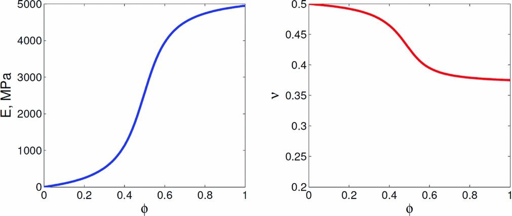
The moduli values Mexp and μexp are measured as a function of time by concurrent Raman and Brillouin light scattering for the pure resin, that is, for a resin curing in the absence of fibres(Reference Heinrich, Alridge, Wineman, Kieffer, Waas and Shahwan42,Reference Aldridge45) . These moduli are assumed to correspond to the virgin matrix as a function of degree of cure. The variation of the Young’s modulus and Poisson’s ratio of the resin, each as a function of cure, is provided in Fig. 1. The Young’s modulus increases from zero to 4,950 MPa at end of cure, whereas the Poisson’s ratio decreases from the incompressibility limit of 0.5 typical of liquid resins to 0.375 at the end of cure. Once M(φ) and μ(φ) are known, the per-network bulk modulus K(φ) can be obtained from the isotropic material relation  $K = M - \frac{4}{3}\mu$.
Young’s modulus (E) and Poisson’s ratio (ν) of the resin as a function of cure (φ) obtained from plane wave modulus and shear modulus data(Reference Heinrich, Alridge, Wineman, Kieffer, Waas and Shahwan42) for Epon 862.
The per-network shrinkage strain εc(Φ) up to a certain degree of cure φ = Φ is given by:
 $$\begin{equation}
\varepsilon _c = \frac{1}{3K(\Phi )}\left[ \left(\varepsilon (\Phi ) - (1 - \Phi )\frac{\text{d}\varepsilon (\Phi )}{\text{d}\Phi }\right) K_{exp} - \frac{\text{d}\varepsilon (\Phi )}{\text{d}\Phi } \int _0^{\Phi } M(\phi )\text{ d}\phi \right]
\end{equation}$$
$$\begin{equation}
\varepsilon _c = \frac{1}{3K(\Phi )}\left[ \left(\varepsilon (\Phi ) - (1 - \Phi )\frac{\text{d}\varepsilon (\Phi )}{\text{d}\Phi }\right) K_{exp} - \frac{\text{d}\varepsilon (\Phi )}{\text{d}\Phi } \int _0^{\Phi } M(\phi )\text{ d}\phi \right]
\end{equation}$$
A gravimetric test method (see Ref. 46) can be used to obtain shrinkage of all networks ε(Φ). A 2% per-network cure shrinkage has been chosen for the present investigation.
2.1 Modelling damage during cure
During curing, the matrix gradually solidifies (stiffness increases) and simultaneously contracts (cure shrinkage) due to network formation. Residual stresses develop in the matrix owing to cure shrinkage and thermal strains. Depending on the magnitude of tensile stresses developed, the degree of cure (φ) and the rate of cure  $(\frac{\text{d}\phi }{\text{d}t})$, the material may crack locally during curing. A crack band model is used to simulate the possibility of tensile cracking during the curing of the matrix. The critical tensile stress for cracking typically increases with the degree of cure. If certain matrix regions crack locally, it would result in a reduction in the matrix stiffness in that local region along with some energy dissipation. Such a reduction in local matrix stiffness can control the mechanical properties of the cured RVE. Two assumptions are enforced because degree of cure and coefficient of thermal expansion of a partially cured local volume with microcracks are unknown and physically this local volume does not represent a continuum in the strictest sense. First, if a certain local volume of material cracks, it is assumed that no further curing can take place in that local volume. Second, it is assumed that if cracking occurs locally, the local cracked volume cannot expand or contract under temperature variations. In the context of the finite element framework that is used to numerically simulate cure-induced damage, this local volume is a single finite element.
At the end of Step I, the curing process is complete. In Step II, the cured RVE (containing cracks or not, as the case maybe) is subjected to transverse tension loading. The objective here is to compute the strength (S +22) and stiffness (E 22) of the virtually cured RVE. Based on the temperature and cure parameters, computation of the stress evolution during cure (Step I) and strength calculation based on mechanical loading (Step II) is performed using the commercial finite element software ABAQUS/Standard (Simulia(47)). In this study, it is assumed that cracking in the curing matrix can occur only for φ > 0.2 and only under tensile stresses.
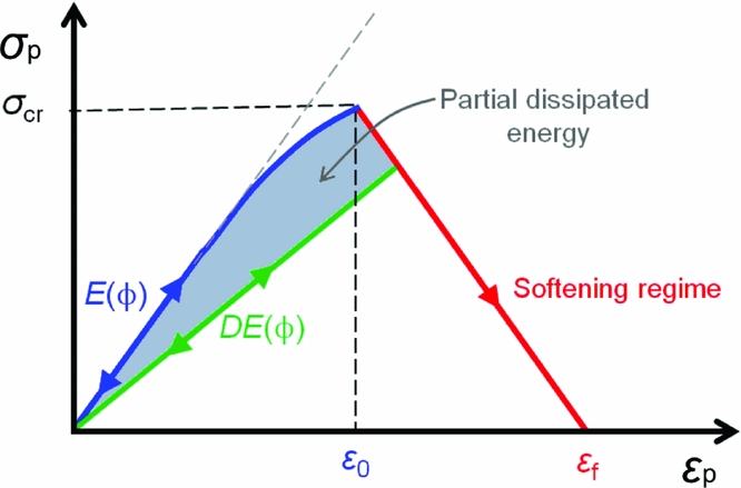
A crack band model based on the one proposed by Bažant and Oh(Reference Bažant and Oh48) is used to model failure in the matrix. This model assumes that once the critical fracture stress σcr is reached, microcracks are formed and this effect is smeared over an element. The maximum principal stress criterion is used to determine the failure initiation in the matrix. However, other failure criteria (such as a mixed Mohr-Coulomb criterion for compressive shear failure) can also be used, based on experimental observations and data that support such. In the present study, when the maximum principal tensile stress exceeds the critical value σcr, the traction-separation law controls the behavior of the damaging material as shown in Fig. 2 and the stiffness of the matrix is reduced using the secant value. In the present investigation, the σcr value is assumed to be independent of φ. However, in reality, it is expected that the strength would vary with φ. Under Mode I cracking, the energy dissipated during the fracturing process is the critical Mode I energy release rate (GIC), given by:
 $$\begin{equation}
G_{IC} = \int _0^{\delta _f} \sigma _{p}(\delta )\text{ d}\delta = h\int _0^{\varepsilon _f} \sigma _{p}(\varepsilon _{p})\text{ d}\varepsilon
\end{equation}$$
$$\begin{equation}
G_{IC} = \int _0^{\delta _f} \sigma _{p}(\delta )\text{ d}\delta = h\int _0^{\varepsilon _f} \sigma _{p}(\varepsilon _{p})\text{ d}\varepsilon
\end{equation}$$
Crack band law in terms of maximum principal stress σp and maximum principal strain εp.

From the crack band model formulation, the stiffness reduction factor due to softening D with (0 ⩽ D ⩽ 1) for a material with initial stiffness E = E(φ), which is now in the softening region of the traction-separation law, is computed as
 $$\begin{equation}
D = \frac{\sigma _{cr}}{E (\varepsilon _f - \varepsilon _{cr})}\left(\frac{\varepsilon _f}{\varepsilon _{p}} - 1\right)
\end{equation}$$
$$\begin{equation}
D = \frac{\sigma _{cr}}{E (\varepsilon _f - \varepsilon _{cr})}\left(\frac{\varepsilon _f}{\varepsilon _{p}} - 1\right)
\end{equation}$$
3.0 RANDOM CELL RVE
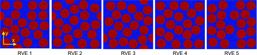
In realistic FRPCs, the fibres are randomly distributed, which give rise to several matrix-rich pockets. It would be instructive to understand the severity of the cure-induced damage on the mechanical response as a function of the randomness in fibre position in an RVE. Eight 3D renditions of square FRPC RVEs with randomly distributed fibres are analysed in this section. The distribution of fibres within the RVEs was done manually, in that, the fibres were arbitrarily placed within the square RVE boundary. The in-plane width of this square RVE is 32 × 10−3 mm, whereas the out-of-plane thickness along the fibre direction is 30 × 10−5 mm. The fibre volume fraction (Vf) in all these renditions is chosen to be 0.55. Each of the RVEs were meshed with C3D8T elements (eight node brick elements with temperature degree of freedom). The fibres are modelled as transversely isotropic solids having radius 3μm, whereas the surrounding matrix material that will undergo curing is modelled as an isotropic solid. These RVEs are shown in Fig. 3. Thermal properties of the fibres and matrix used in these computations are provided in Table 1. Few strategies to generate random RVEs may be found in the works of Melro et al(Reference Melro, Camanho and Pinho50), Yang et al(Reference Yang, Ying, Ran and Liu51) and Vaughan and McCarthy(Reference Vaughan and McCarthy52). Recently, using a heuristic random microstructure algorithm, Romanov et al(Reference Romanov, Lomov, Swolfs, Orlova, Gorbatikh and Verpoest53): have generated RVEs that are statistically well correlated with real FRPC RVEs.
Five renditions of random 20-fibre RVEs with volume fraction Vf = 0.55.
Thermal properties of the fibres and matrix

3.1 Boundary conditions
During curing and mechanical loading, the RVE is subjected to periodic boundary conditions, in concert with the assumption that the RVE is a small volume within an infinite medium. The use of periodic boundary conditions for fibre-reinforced RVEs can be found in the studies of Gonzalez and Llorca(Reference Gonzalez and Llorca54) and Xia et al(Reference Xia, Zhang and Ellyin55), amongst others. During the cure process, the RVE can contract or expand depending on temperature change and can contract due to cure shrinkage.
Consider an arbitrary cuboid RVE in the undeformed configuration having lengths L 1, L 2 and L 3 along the x 1, x 2 and x 3 directions with one corner point placed at the origin (0, 0, 0). Then, the equations corresponding to the 3D periodic boundary conditions are:
 $$\begin{eqnarray}
u_{1}(L_{1}, x_{2}, x_{3}) - u_{1}(0, x_{2}, x_{3}) &=& \varepsilon _{11} L_{1}, \nonumber\\
u_{2}(L_{1}, x_{2}, x_{3}) - u_{2}(0, x_{2}, x_{3}) &=& 2\varepsilon _{12} L_{1}, \nonumber\\
u_{3}(L_{1}, x_{2}, x_{3}) - u_{3}(0, x_{2}, x_{3}) &=& 2\varepsilon _{13} L_{1}, \nonumber\\
u_{1}(x_{1}, L_{2}, x_{3}) - u_{1}(x_{1}, 0, x_{3}) &=& 2\varepsilon _{21} L_{2}, \nonumber\\
u_{2}(x_{1}, L_{2}, x_{3}) - u_{2}(x_{1}, 0, x_{3}) &=& \varepsilon _{22} L_{2}, \\
u_{3}(x_{1}, L_{2}, x_{3}) - u_{3}(x_{1}, 0, x_{3}) &=& 2\varepsilon _{23} L_{2}, \nonumber\\
u_{1}(x_{1}, x_{2}, L_{3}) - u_{1}(x_{1}, x_{2}, 0) &=& 2\varepsilon _{31} L_{3}, \nonumber\\
u_{2}(x_{1}, x_{2}, L_{3}) - u_{2}(x_{1}, x_{2}, 0) &=& 2\varepsilon _{32} L_{3}, \nonumber\\
u_{3}(x_{1}, x_{2}, L_{3}) - u_{3}(x_{1}, x_{2}, 0) &=& \varepsilon _{33} L_{3},\nonumber
\end{eqnarray}$$
$$\begin{eqnarray}
u_{1}(L_{1}, x_{2}, x_{3}) - u_{1}(0, x_{2}, x_{3}) &=& \varepsilon _{11} L_{1}, \nonumber\\
u_{2}(L_{1}, x_{2}, x_{3}) - u_{2}(0, x_{2}, x_{3}) &=& 2\varepsilon _{12} L_{1}, \nonumber\\
u_{3}(L_{1}, x_{2}, x_{3}) - u_{3}(0, x_{2}, x_{3}) &=& 2\varepsilon _{13} L_{1}, \nonumber\\
u_{1}(x_{1}, L_{2}, x_{3}) - u_{1}(x_{1}, 0, x_{3}) &=& 2\varepsilon _{21} L_{2}, \nonumber\\
u_{2}(x_{1}, L_{2}, x_{3}) - u_{2}(x_{1}, 0, x_{3}) &=& \varepsilon _{22} L_{2}, \\
u_{3}(x_{1}, L_{2}, x_{3}) - u_{3}(x_{1}, 0, x_{3}) &=& 2\varepsilon _{23} L_{2}, \nonumber\\
u_{1}(x_{1}, x_{2}, L_{3}) - u_{1}(x_{1}, x_{2}, 0) &=& 2\varepsilon _{31} L_{3}, \nonumber\\
u_{2}(x_{1}, x_{2}, L_{3}) - u_{2}(x_{1}, x_{2}, 0) &=& 2\varepsilon _{32} L_{3}, \nonumber\\
u_{3}(x_{1}, x_{2}, L_{3}) - u_{3}(x_{1}, x_{2}, 0) &=& \varepsilon _{33} L_{3},\nonumber
\end{eqnarray}$$
where u 1, u 2, and u 3 are the displacements of the RVE boundary along the x 1, x 2 and x 3 directions, respectively, and εij are the tensorial strains.
3.2 Analysis procedure for virtual curing of random cell RVEs
The analysis procedure is divided into two steps as described below.
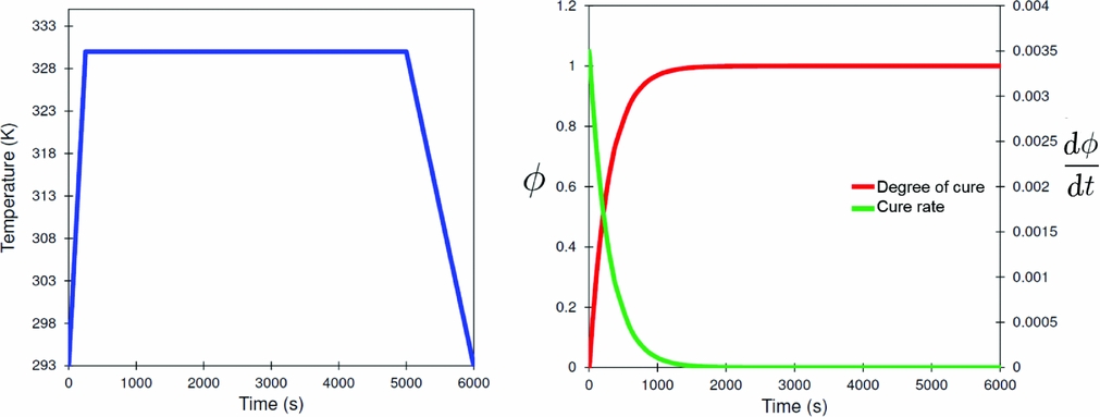
(1) Step I: A thermochemical analysis is performed using the cure parameters described earlier. The temperature cycle, the degree of cure, and the cure rate in the matrix are provided. Since the RVE dimensions are on the micron scale, there is little to no variation in the temperature field across the RVE. The temperature profile, the degree of cure (φ) and the rate of cure
$(\frac{\text{d}\phi }{\text{d}t})$ used in the present study are shown in Fig. 4. The stress evolution calculations are performed as described in Equation (5). Shrinkage during cure is modelled using Equation (7). At the end of this step, we have a virtually cured solid. The possibility of damage during curing is taken into account using the crack band model. Periodic boundary conditions are enforced throughout this step. The present step is implemented as a coupled temperature-displacement analysis.
Figure 4.Temperature cycle (left) along with degree of cure (φ) and rate of cure (
$\text{d}\phi /\text{d}t$) (right).(2) Step II: Each of the virtually cured RVEs is subjected to transverse tensile loading (with periodic boundary conditions in place) to back-out the stiffness and strength. Again, the crack band model is used to simulate tensile failure in the matrix. The material state at the beginning of this step is the one that was obtained at the end of Step I. The reference configuration for this step is taken as the deformed configuration of the cured RVE (i.e. corresponding to end of Step I). Hence, the constitutive law for the RVE during the mechanical loading step is
where [C] is the current stiffness matrix, εm are the applied mechanical strains, and σ0 are the self-equilibrating residual stresses present in the virtually cured RVE. Note that at the start of Step II, when εm = 0, then, σ = σ0. Thus, the additional stress buildup in the structure during mechanical loading is caused by the applied mechanical strains εm during transverse tensile loading.(11)
$$\begin{equation}
\bm {\sigma } = [C]\bm {\varepsilon }_{m} + \bm {\sigma }_0,
\end{equation}$$


3.3 Results
When each of the five RVEs are subjected to the cure cycle, self-equilibrated stresses are generated governed by the network model, cure shrinkage and thermal mismatch. In particular, predominant tensile stresses develop due to cure shrinkage when the polymer networks form during the initial stages of the cure cycle during the first 1,500s of the cure cycle. Additional tensile stresses develop during the cooling phase of the cure cycle (5,000s < t < 6,000s ). The contour plots of the maximum principal stresses generated in the matrix at the end of the cure cycle are shown in Fig. 5.
Contours of maximum principal stresses (MPa) in the RVE matrix at the end of the cure cycle.
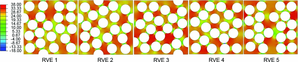
The magnitude and distribution of the residual stresses in each of the five RVEs are different owing to the difference in fibre packing. Maximum principal stresses up to 38 MPa are generated at the end of cure in these RVEs. Since the magnitude of tensile stress in the curing matrix did not exceed its critical fracture stress σcr at any stage of the cure cycle, no damage/cracking is observed.
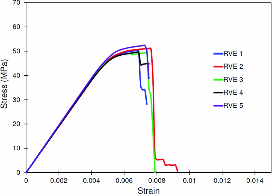
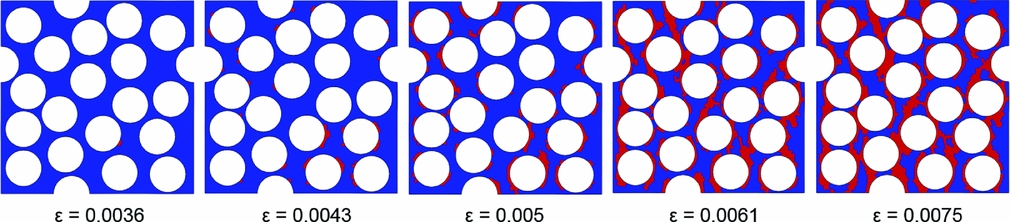
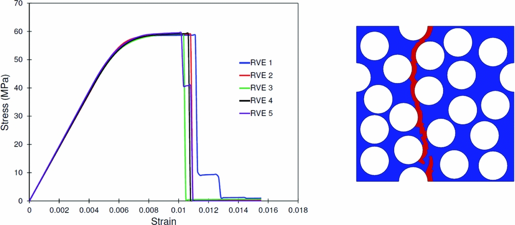
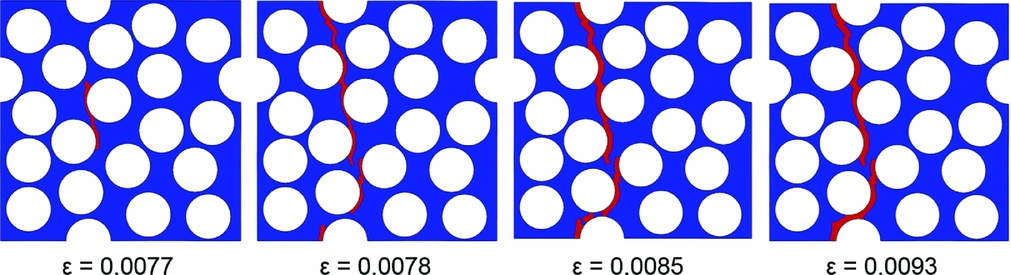
The virtually cured random RVEs are next subjected to transverse tension loading (Step II). The resulting nominal stress-strain response is provided in Fig. 6. Each of the stress-strain responses initially exhibits a linear response up to a nominal strain value of 0.005, after which there is slight pre-peak nonlinearity in the response followed by a drop in stress. This pre-peak nonlinearity begins when microcracks initiate in the matrix at some location at the fibre matrix interface that has high-stress gradients. With further loading, these microcracks form at other locations in the RVE causing further reduction in stiffness. Using RVE 2 for illustration, the sequence of microcrack formation at various stages of loading is shown in Fig. 7. These microcracks spread until a prominent two-piece crack develops, which causes the load to drop past the peak. For RVE 2, the sequence of two-piece crack formation that begins at the peak stress is shown in Fig. 8. The peak values, which denote the RVE strength S +22, are somewhat different from one another, averaging 50.5 MPa with minimum and maximum strength values of 49.4 MPa and 52.3 MPa, respectively.
Nominal stress-strain (σ22 − ε22) response of the virtually cured random RVEs when subjected to transverse tension loading.

Initiation and spread of microcracks in RVE 2 that leads to deviation from linearity in the stress-strain response prior to two-piece cracking. The microcracks are shown in red.

Initiation and rapid growth of two-piece cracking (in red) in the RVE which starts and proceeds past the peak in RVE 2.
Another set of transverse tension simulations were performed using each of the five random RVEs, but where the effect of curing was neglected. That is, each of the RVEs was modelled as an initially stress-free solid with matrix properties equal to that of neat resin, i.e. Young’s modulus 4,950 MPa and Poisson’s ratio 0.375. The objective is to estimate the difference between the transverse strength S +22 if one does not take into account the effect of processing (virtual curing). The nominal stress-strain responses of each of the RVEs when processing effects are neglected, are shown in Fig. 9. The corresponding two-piece crack paths past the peak stress for RVE 2 is shown in Fig. 9. Like the earlier set of simulations with virtually cured RVEs, the deviation from linearity is controlled by initiation and spread of microcracks in the RVE and the peak is controlled by two-piece crack formation. The average S +22 strength is 59 MPa with very little spread – the minimum and maximum values are 58.7 MPa and 59.5 MPa, respectively. The strength values observed in these simulations are noticeably higher than those seen from the mechanical loading of virtually cured RVEs. This observation is expected due to the presence of self-equilibrating residual stresses present in the virtually cured RVEs, a portion of which are tensile in nature. Although the transverse strength values are found to be different, the transverse stiffness (E 22) measurements between these two sets of simulations are identical because no stiffness reduction was seen in the RVEs at the end of cure for the set of matrix properties used here. A different set of properties can lead to stiffness reduction during the curing.
Nominal stress-strain (σ22 − ε22) response of random RVEs when subjected to transverse tension loading (left). Two-piece crack path shown in red for RVE 2.

4.0 PLAIN WEAVE RVE
4.1 Introduction
The second type of composite structure that will be subjected to curing is a plain weave RVE. The plain weave is the simplest of composite textile architecture where warp and weft tows undulate over one another successively. Fairly accurate estimates for the effective stiffness properties for the plain weave architecture can be found using analysis models for textile composites, for example, by Quek et al(Reference Quek, Waas, Shahwan and Agaram56) and Kier et al(Reference Kier, Salvi, Theis, Waas and Shahwan57).
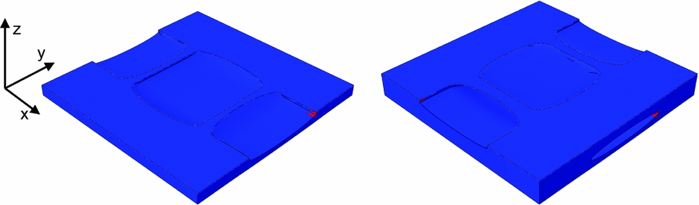
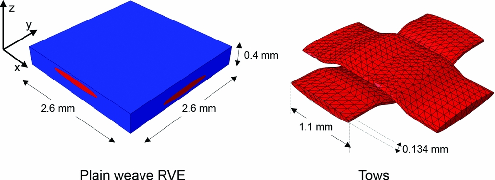
The geometry of the plain weave RVE used in the present work is given in Fig. 10. In this RVE, the tow volume fraction is 0.28. The in-plane width of the RVE is 2.6 mm and the out-of-plane thickness is 0.4 mm. The RVE is meshed with 24,244 quadratic tetrahedral elements having temperature degrees of freedom.
Plain weave RVE (left) with matrix shown in blue and tows shown in red; constituent tows (right) with dimensions. Here,  $x\text{-}y\text{-}z$ axes indicate the global reference frame.
Similar to the earlier case with random fibre RVEs, the analysis of the plain weave RVE in this work is done using two steps. That is, in Step I, the plain weave RVE is subjected to the cure cycle where the matrix between the tows undergoes curing. In the present work, the tows are assumed to have already cured. The possibility of curing of the tow simultaneously with the surrounding matrix is a subject of an ongoing study. During the cure process, the in-plane boundaries are constrained to remain flat. That is, the faces having normals pointing along x or y are held flat, but are allowed to contract/expand. At the end of Step I, we have a virtually cured plain weave RVE, which is subsequently subjected to tensile loading along the x direction in Step II. A dynamic/explicit solver is used to execute Step II. In this step, the flat boundary conditions are relaxed and the structure is loaded under uniaxial conditions. Throughout the analysis, damage and failure in the matrix is modelled using the crack band approach discussed earlier. The fracture parameters for the matrix in the plain weave RVE are taken to be similar to the one used in the earlier analysis on random fibre RVEs, i.e. critical fracture stress σcr = 60 MPa and mode I fracture toughness GIC = 0.2 N/mm. In order to simulate failure in the tow, a multiscale model developed by Zhang and Waas(Reference Zhang and Waas58) is used, which is briefly described below.
4.2 Tow damage model
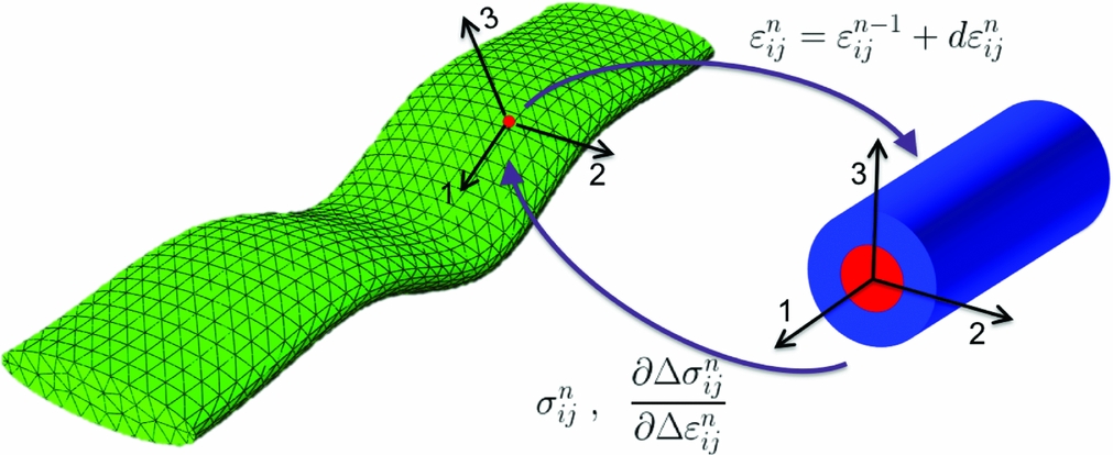
The plain weave tow is modelled as a transversely isotropic solid. The tow, which is essentially a fibre bundle held together by matrix, is assumed to have fibre volume fraction of 0.64. The two-scale model proposed by Zhang and Waas(Reference Zhang and Waas58), which models the behaviour of the tow, considers a Concentric Cylinder Model (CCM) representation at each integration point of the homogenised tow. The CCM calculates the effective transversely isotropic properties of fibre composites in terms of matrix elastic properties, fibre transversely isotropic properties, and fibre volume fraction. The two scales thus involved are the mesoscale tow (homogenised as transversely isotropic solid) and the microscale CCM that sits at each integration point of the mesoscale tow. When global strains are applied on the textile composite RVE, strains in the mesoscale tow at each integration point are passed to the CCM at the microscale. Using closed form expressions for the CCM, as shown in Zhang and Waas(Reference Zhang and Waas58), the stresses and material Jacobian are passed back (see Fig. 11) to the mesoscale at each integration point after updating. That is, at the CCM microscale, decisions are made predicated on the criticality of stresses (or strains as the case may be) regarding damage and failure development in the tow(Reference Zhang, Waas and Yen33).
Methodology of the model proposed by Zhang and Waas(Reference Zhang and Waas58). For a given integration point on the mesoscale tow model, strains are passed to the CCM at the microscale; updated stress and current Jacobian get passed back from the microscale to the mesoscale at the end of an increment. The 1-2-3 axes represent local material orientation, where direction-1 points along the fibre direction.

In the present computations, if the stresses at the integration point exceed critical values, then damage in the tow at that corresponding integration point is modelled using a smeared crack approach (SCA). In the tow, when tensile stresses along the axial direction exceed a critical value σtow, +cr, the softening response is modelled using the smeared crack approach. The aforementioned failure mode occurs due to axial tow fracture, which is controlled by fibre failure strain. Other secondary tow failure modes such as transverse tow cracking are not considered in the present work, and are the subject of ongoing research.
The constituent fibre properties are provided in Table 2. The tow’s constituent matrix isotropic properties are assumed to be similar to that of a completely cured Epoxy resin, i.e. Young’s modulus 4,950 MPa, Poisson’s ratio 0.375, critical fracture stress σcr = 60 MPa, and mode I fracture toughness GIC = 0.2 N/mm.
Constituent properties of the fibres in the tow along with thermal and fracture properties of the tow

4.3 Analysis
The RVE shown in Fig. 10 is subjected to the cure cycle shown in Fig. 4. Residual stresses are generated in the RVE due to temperature changes as well as due to cure shrinkage in the matrix. At the end of the cure cycle (Step I), the state of maximum principal residual stress in the matrix is shown in Fig. 12. It is seen that this stress state is nonhomogenous over the matrix elements and is uniformly higher in magnitude at the centre of the RVE compared to regions near the boundaries along the x and y directions. Note that at the centre of the RVE, the matrix is in a region where the tows cross over. Moreover, the stresses are high in the matrix in this region, where stress gradients are also high. Matrix damage was observed in few elements in such regions. The damage occurring in a few elements is highlighted in red in Fig. 13.
Contours of the maximum principal stress (MPa) in the matrix: entire RVE (left) and slice taken at mid height (right).
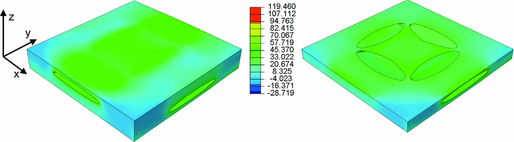
Sectioned images of the deformed RVE; a cut through the middle of the RVE and parallel to the  $x\text{-}y$ plane. Matrix damage that occurs during the curing process is highlighted in red.

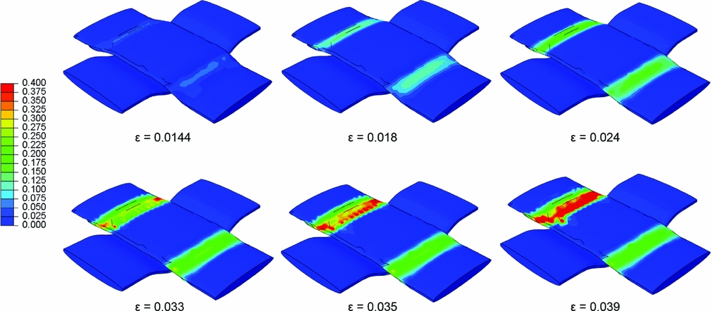
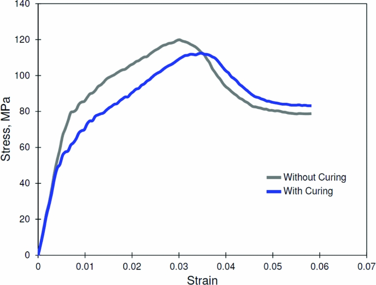
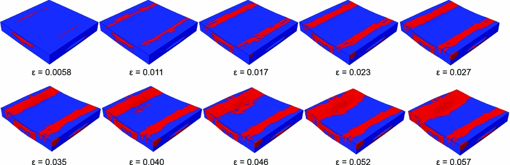
The virtually cured plain weave RVE is loaded in tension along the x direction. The nominal stress-strain response, which indicates progressive damage and failure, is shown in Fig. 14. During the initial stages of loading, a relatively stiff linear region is encountered up to a nominal strain value of 0.005, after which there is some reduction in stiffness up to a peak stress of 112 MPa, followed by a drop. The reduction in stiffness following the nominal strain value of 0.005 occurs due to straightening of the tow with simultaneous matrix cracking in regions adjacent to the tow, whereas the peak is controlled by axial tow failure. Figure 15 shows the sequence of matrix cracking at various stages of loading. Note that two-piece cracking has initiated as two separate bands immediately after a strain value of 0.005 (where stiffness reduction is seen in the stress-strain response), with each band growing with additional loading. Figure 16 shows the growth and localisation of maximum principal strains in the tows during the mechanical loading step.
Nominal stress-strain response of the virtually cured plain weave RVE under in-plane tensile loading along with stress-strain response of plain weave RVE under in-plane tensile loading when curing is not taken into account.
Evolution of tensile cracking in the matrix during the mechanical loading of the virtually cured plain weave RVE.
Contours of maximum principal strains in the tows of the virtually cured plain weave RVE, shown at various stages corresponding to global tensile strain values.

PaInitially, as the tow parallel to the loading direction begins to straighten out, two prominent bands of strain localisation start to form at the tow inflection site. As the tow further straightens out, the magnitude of straining in these regions also increases. At a nominal strain value of 0.035, axial tow fracture occurs in one of the localisation bands, which is reflected by a sudden jump in the strain values. Note that the peak stress in the stress-strain response also occurs around the nominal strain value 0.035, which suggests that axial tow fracture is the mechanism that controls the peak stress for this plain weave RVE. From this computation, it is seen that the maximum tensile strength of the composite plain weave RVE is approximately 112 MPa. We also performed a simulation on the plain weave RVE when it was not subjected to curing. That is, the RVE is assumed to be initially stress-free and having matrix property of the neat resin (Young’s modulus 4,950 MPa and Poisson’s ratio 0.375). This RVE is also loaded in tension along the x direction. The resulting stress-strain response is shown in Fig. 14 alongside the response of the virtually cured plain weave RVE. The tensile strength of this RVE is 119 MPa compared to 112 MPa for the virtually cured RVE. Moreover, the initial linear response is longer, and the departure from linearity into the prepeak regime due to crack initiation is delayed in this RVE, occurring at a higher strain value. Thus, the presence of residual stresses due to curing is seen to somewhat reduce the strength of the virtually cured RVE. Using this ICME modelling framework, other strength values such as compressive strength, in-plane and out-of-plane shear strengths, and transverse compressive strength can be computed and the relative influence of microstructural parameters on these strengths can be quantified. Therefore, uncertainties associated with the relative magnitudes of microstructural variables can be quantified using the present ICME modelling framework.
5.0 CONCLUSIONS
This paper has addressed a subject that is emerging and important for future certification of aerostructures in a timely manner. With several advances in cost-effective production of composite aerostructures, the need to have reliable, high-fidelity and computationally efficient virtual tools for composite aerostructures is urgent. ICME tools will become the mainstay for rapid insertion of new high-performance structural concepts in an affordable manner. Within the ICME framework, the effects of cure cycle on the subsequent mechanical response of a fibre-reinforced pre-preg lamina and a plain weave textile composite have been presented. It is seen that the curing process influences the subsequent effective stiffness and strength of the studied structures when subjected to mechanical loading. This is because the matrix material, depending on details of the cure cycle, and fracture and strength properties, which are also dependent on details of the cure cycle, can undergo microcracking due to internal residual stresses. When subjected to mechanical loads, these stresses get added to additional stresses generated due to applied mechanical loads. Fiber packing is seen to influence the details of damage development. There is a non-negligible effect on predicted ply strengths and plain weave strengths if details of the cure cycle are not included in the RVE level analysis models. An assembly of RVEs that have the softening response shown here would need to be modelled in order to make comparisons against experimental, coupon level data. That is an ongoing task.
ACKNOWLEDGEMENTS
The authors are grateful for the involvement of many who have enhanced our understanding of the effects of cure. We acknowledge Dr Li Zheng, Dr Folusho Oyerokun, Matthew Hockemeyer, Dr Lara Liou, and Dr Thomas Sutter of General Electric; Dr Steve Engelstad and Dr Bob Koon of Lockheed Martin; Dr G P Tandon of University of Dayton Research Institute, and Dr Eric Baker, Dr Kevin Kendig, and Dr Greg Schoeppner from Air Force Research Laboratory.