


1. Introduction
Modelling is essential to every aspect of life and health insurance. Pricing and expenses management depend on credible estimates of mortality and morbidity across various factors. Compared to non-life actuaries, life & health data sets pose distinct challenges: mortality and morbidity events are rare (especially at younger ages), exposure at specific segments is thin, and credible factor interactions quickly fragment claim counts into sparsely populated cells. As a result, actuaries face a persistent balancing act between model richness and statistical credibility.
Over time, the GLM toolkit has been expanded with shrinkage (e.g. LASSO, Ridge and elastic net) and smoothing techniques (e.g. GAMs and polynomials) to control variance, reduce noise, and avoid overfitting; yet the fundamental use of GLM has changed little in day-to-day practice. This persistence reflects the transparency, interpretability, and governance readiness of GLMs, which remain central to actuarial validation, communication, and review. However, these strengths come at the cost of a limited ability to capture complex nonlinearities and interactions without substantial manual effort.
In parallel, machine learning (ML) techniques, including gradient boosting machines and neural networks, have seen rapid development, and offer a powerful alternative to GLMs by automatically capturing complex nonlinearities and variable interactions without a priori specification. Compared to these novel models, various authors have shown that traditional GLMs can leave value on the table (Bjerre, Reference Bjerre2022; Richman & Wüthrich, Reference Richman and Wüthrich2021). However, uptake has been limited due to regulatory scrutiny, difficulties in interpretation and privacy challenges (CAS Machine Learning Working Party, 2022).
Rather than viewing ML as an alternative to traditional actuarial models, the actuarial literature has largely focused on enhancing traditional models using ML. A wide range of approaches for enhancing GLMs using ML have been proposed (CAS Machine Learning Working Party, 2022). One strand uses ML for feature engineering, including identifying nonlinearities, clustering or binning (Dai, Reference Dai2018; Henckaerts et al., Reference Henckaerts, Antonio, Clijsters and Verbelen2018; Maillart, Reference Maillart2021). A second strand uses ML as a diagnostic or exploratory tool to detect nonlinearities and/or interactions for a subsequent GLM-like model (Tam & Luteijn, Reference Tam and Luteijn2025). A third strand uses ML to directly correct for signal not captured by a baseline model (Gawlowski & Wang, Reference Gawlowski and Wang2025). These approaches aim to preserve transparency whilst leveraging the predictive power of ML models and are typically evaluated in isolation, using different data sets and performance metrics. As a result, actuaries lack clear guidance on how these hybrid approaches compare in terms of predictive performance, transparency, governance readiness, and modeller control required for practical deployment.
Mortality data provides a useful methodological case study for informing a broader range of life and health actuarial modelling problems. The gap between traditional methods and ML methods is especially evident in health and care insurance, where the literature on ML models proposes to replace rather than augment GLM-based frameworks (Kshirsagar et al., Reference Kshirsagar, Hsu, Greenberg, McClelland, Mohan, Shende, Tilmans, Guo, Chheda, Trotter, Ray and Alvarado2021; Orji & Ukwandu, Reference Orji and Ukwandu2023). The challenges faced in health and care modelling share many aspects with those faced in mortality modelling.
In this paper, we address this disconnect by appraising three hybrid additive modelling approaches that integrate gradient boosting into an additive model framework to support practical adoption in actuarial practice. Specifically, we evaluate three approaches drawn from the latter two strands described earlier: interpretable boosted linear models using XGboost to correct a baseline GLM model (Gawlowski & Wang, Reference Gawlowski and Wang2025); an interaction detection framework in which gradient boosting is used to detect interactions (Tam & Luteijn, Reference Tam and Luteijn2025); and an XGBoost-informed GLM approach where gradient boosting insights guide manual feature engineering. The focus on gradient boosting is informed by the observation that gradient boosting is state-of-the-art for tabular data (Grinsztajn et al., Reference Grinsztajn, Oyallon and Varoquaux2022). The contribution of this paper is methodological rather than outcome-specific, focusing on governance-ready additive model structures rather than mortality estimation per se.
2. Methods
2.1. Objective
The objective of this paper is to assess how different hybrid approaches that integrate gradient boosting into additive actuarial models perform across predictive accuracy, transparency, governance readiness, and modeller control. The focus is on approaches that retain an explicit additive structure suitable for actuarial deployment, rather than fully automated black-box models.
To support a fair and reproducible comparison, all approaches are evaluated using a common data set and consistent performance metrics. Baseline GLM-type models, black-box XGBoost benchmarks, and three hybrid approaches are considered to contextualise performance trade-offs.
2.2. Data Set
We performed analysis on American life insurance experience data, publicly available via the Individual Life Insurance Experience Committee (ILEC) of the Society of Actuaries (SoA) (Individual Life Insurance Experience Committee of the Society of Actuaries, 2024), which we will refer to as the ILEC data.
The ILEC data set was selected for its public availability (allowing anyone to reproduce our study), large size (273,402 claim counts), documentation and relevance to insurance. The ILEC data covers American life insurance experience over observation years 2012–2019.
2.2.1 Data Pre-processing
Inclusion criteria were term business only, attained age between 18 and 90, issue age between 18 and 80, issue years 1980 onwards and duration up to 20. Entries with unknown smoking status were excluded as experience was very heavy (197% on the ILEC-supplied expected basis), raising concerns over data quality. Following these data filters, the data set contained 273,402 claims with an average claim size of $292,000 over 160.18 million life years.
Amongst the features within the data set, Observation_Year, Sex, Smoker_Status, Duration, Face_Amount_Band and Attained_Age were considered for mortality modelling. Features excluded for simplicity included features around preferred ratings and product types that may not necessarily translate to UK settings. There were no missing values for any of the features utilised.
We noted that age was reported either on an Age Last Birthday (ALB) or an Age Nearest Birthday (ANB) basis. The life year exposure proportions of ALB and ANB are approximately 44% and 56%, respectively. However, we do not have the granularity to align the two bases in an exact manner. Although we can approximate alignment by adding 0.5 years to the ages of rows with ANB, this comes with undesirable complications as there is material difference between ALB and ANB business not explained by age. For simplicity, no adjustments were made. We do not anticipate any material impact on our analysis.
2.2.2 ILEC VBT 2015
The ILEC data set comes with expected claim counts, based on the 2015 valuation base table (VBT 2015). VBT 2015 rates were produced by ILEC on 2002–2009 experience data and extended to 2015 using mortality improvement assumptions. (Academy/SOA Valuation Basic Table Team, 2018).
2.2.3 Partitioning
To evaluate model performance, two data partitions were modelled. In the first partition, the data set was randomly split by row into training (80%) and test (20%) subsets. In the second partition, the final two observation years (2018 and 2019) were test data, whilst 2012–2017 were training data. The random split results in a test data set more like the training data than the observation year partition. Partitioning test data by observation year more closely aligns with actuarial practice of using historic experience to forecast future experience.
For the IBLM XGBoost booster model, the training subset was further divided using random sampling into an internal training set (80%) and a validation set (20%). This secondary split was used for early stopping. The XGBoost models used for interaction detection (models 4 and 5) were trained using cross-validation so no further partitioning was required.
2.3. Predictive Models
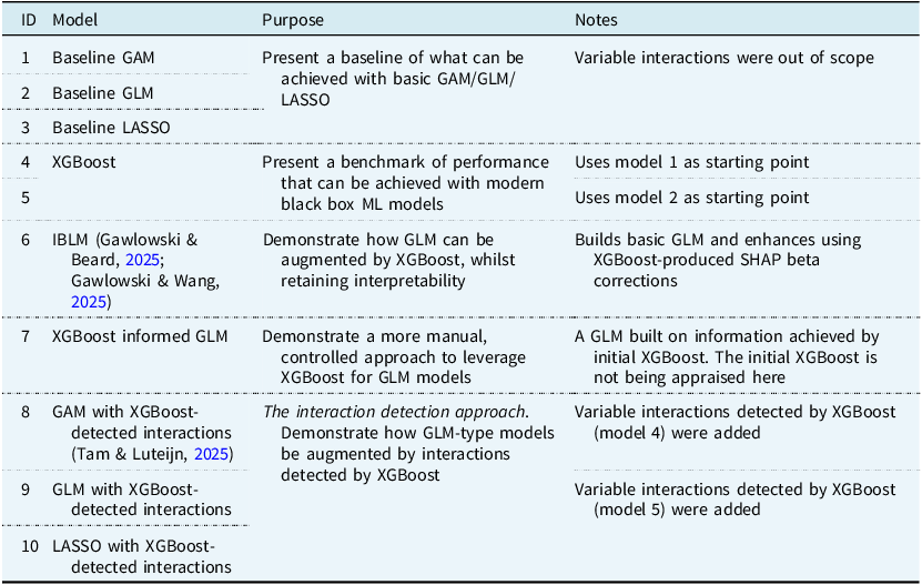
Baseline performance was quantified using Poisson GAM, GLM, and LASSO models, whereas performance of modern black-box approaches was quantified using two XGBoost models (Table 1, models 1–5). Finally, five models representing the three hybrid GLM-GBM approaches were trained (Table 1, models 6–10).
Models evaluated

Table 1. Long description
The table compares various models used for baseline performance and modern black-box approaches. It includes ten models categorized by their purpose and notes. The first three models are baseline models using GAM, GLM, and LASSO. The next two models are XGBoost models used as benchmarks. The remaining five models represent hybrid GLM-GBM approaches. Each row details the model ID, type, purpose, and specific notes. The table provides a structured overview of the models’ roles and enhancements, focusing on their performance and interpretability.
The GAM models (1, 4 and 8) were trained in Python and the remaining models (2–3, 5–7 and 9–10) were trained in R. The entire work is publicly available via GitHub (IFoA Techniques in Data Science in Health and Care, 2026). For readers unfamiliar with some of the terminology and methodology discussed here, we refer to our recently published framework for applying data science techniques to health and care actuarial projects. (Luteijn et al., Reference Luteijn, Tam, Denis, Fan, Minhas, Puthanveedu and Takyi2026)
The two previously published strategies demonstrated here are based on the interaction detection approach (Tam & Luteijn, Reference Tam and Luteijn2025) (models 8–10) and the Interpretable Boosted Linear Model (IBLM), model 6 (Gawlowski & Wang, Reference Gawlowski and Wang2025). The third strategy, model 7, is a more manual approach to leverage SHAP dependence plots for determining GLM regression formulae. The Poisson distribution was used for the sake of simplicity for all ten models.
2.3.1 Baseline Models
All baseline models used combinations of polynomials and splines to model nonlinearities within the numeric features. Variable interactions were outside the scope of the baseline models as interactions will be addressed by the boosting machines further downstream. For the GAM, hyperparameters were selected using cross-validated Bayesian tuning.
2.3.2 XGBoost Models
Two XGBoost models were trained targeting claim counts, offset by the log of baseline GLM/GAM predictions, respectively (Table 1, models 4 and 5). Therefore, the XGBoost effectively targets the remaining signal in the log claim rate unexplained by the GAM/GLM predictions (similar to the internal XGBoost booster model in the IBLM, Section 2.3.4).
Cross-validation was used to prevent overfitting. Hyperparameter tuning was performed on model 4 using Optuna (Akiba et al., Reference Akiba, Sano, Yanase, Ohta and Koyama2019) and the calibrated set of hyperparameters were also applied to XGBoost model 5 and the internal IBLM model. Tree depth for the XGBoost models was set to two to restrict variable interactions to first-order interactions to support the interaction detection approach (Section 2.3.3).
2.3.3 GLM-GBM Hybrid Approaches
Three hybrid approaches were applied: (1) the Interpretable Boosted Linear Model (Gawlowski & Wang, Reference Gawlowski and Wang2025); (2) the interaction detection approach (Tam & Luteijn, Reference Tam and Luteijn2025); and (3) an XGBoost-informed GLM. These three approaches selected apply different levels of automation to the process of improving additive model performance using XGBoost. All three approaches produce a final additive model that is suitable for actuarial deployment.
Interpretable Boosted Linear Model
The IBLM (Table 1, model 6) combines a traditional GLM model with an XGBoost (Gawlowski & Wang, Reference Gawlowski and Wang2025). This is achieved via a sequential approach: first, a basic GLM is fitted without feature engineering or variable interactions. Subsequently, an XGBoost model is tasked with capturing patterns the GLM failed to capture by targeting the residuals of the training data against the GLM predictions. The corrections by the XGBoost model can be approximated by a GLM-like structure by absorbing zeroes and reference levels of category features into the intercept. The IBLM package code (Gawlowski & Beard, Reference Gawlowski and Beard2025) was updated by adding an offset (life years exposure) to the GLM and weighting the XGBoost training by life years exposure. The IBLM model by default uses a tree-depth of three. To facilitate comparison with models that do not accommodate third-order interactions, and because interpretability of third-order interaction is limited, the IBLM was additionally trained using a tree depth of two.
Interaction Detection Approach
The interaction detection approach (Tam & Luteijn, Reference Tam and Luteijn2025) involves building a baseline additive model without feature interactions. The residuals of the baseline model are targeted by XGBoost and top- ranking feature interactions identified by XGBoost are incorporated back into a final additive model built from scratch (Table 1, models 8–10). This strategy was tested with GAM, GLM and LASSO models. Both the GLM and LASSO use a GLM baseline since shrinkage was not considered desirable for setting a starting point.
XGBoost-Informed GLM
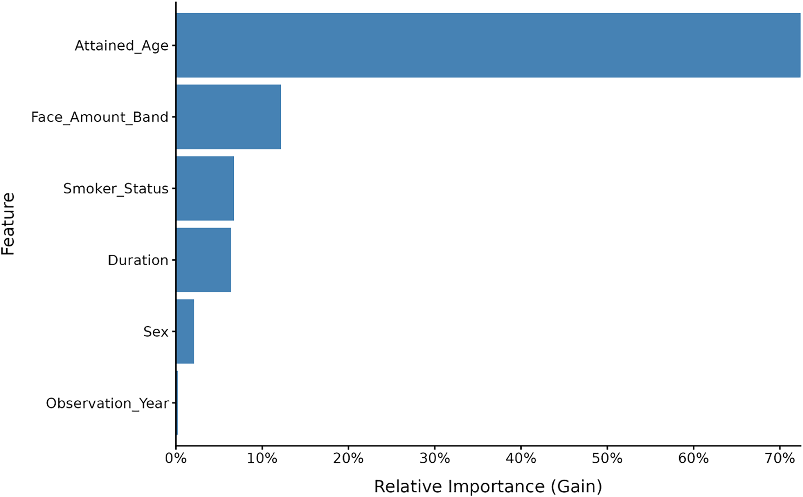
The XGBoost-informed GLM (Table 1, model 7) was trained by first fitting an XGBoost on the training data, targeting claim counts with lives exposure as an offset. The feature importance plot of this XGBoost is included in Figure 1. A final GLM was then built using a regression formula informed by XGBoost-derived visuals.
XGBoost normalised feature importance by gain.

Figure 1. Long description
A horizontal bar graph displays the relative importance of various features by gain. The x-axis represents the relative importance in percentage, ranging from 0 to 70 percent. The y-axis lists the features: Attained Age, Face Amount Band, Smoker Status, Duration, Sex, and Observation Year. Attained Age has the highest relative importance at approximately 70 percent. Face Amount Band follows with around 10 percent. Smoker Status and Duration each have a relative importance of about 5 percent. Sex and Observation Year have the lowest relative importance, each below 5 percent. The bars are colored in blue, with varying lengths corresponding to their relative importance values. All values are approximated.
For example, attained age is by far the most important feature in the XGBoost (Figure 1), which suggests that using a spline to fit the age curve could be the most impactful. Its SHAP dependence plot shows a smooth but highly nonlinear variation in SHAP values across age (Figure 2). This suggests that a simple linear term would severely underfit this relationship. The SHAP curve shows a dip at approximately ages 25–33, followed by multiple changes in curvature around ages 45, 55, and 70 as the marginal effect of age accelerates at older ages. Placing knots at 25, 33, 45, 55, and 70 thus allows the spline to capture this data-driven curvature, rather than relying on evenly spaced knots or quantile-based placement.
SHAP dependence plot for attained age.

Figure 2. Long description
A scatter plot showing the SHAP value for attained age against attained age with a red trend line. The x-axis represents attained age, ranging from 0 to 90 years. The y-axis represents the SHAP value for attained age, ranging from -2 to 2. The plot contains hundreds of data points, which are black dots. The red trend line indicates a positive correlation between attained age and SHAP value, showing an upward trend as attained age increases. The data points are densely clustered around the trend line, with some variability. All values are approximated.
2.4. Appraisal Framework
Having outlined the three modelling approaches, this section will describe the appraisal framework by which they will be assessed (Table 2).
Hybrid approach assessment criteria

Table 2. Long description
A table with four rows and three columns compares hybrid approach assessment criteria. The columns are labeled Assessment criterion, Evaluation metric, and Section. The rows detail Predictive performance with Mean Poisson deviance improvement on test splits, Modeller control with Degree of manual intervention required, Transparency with Final model additive structure and ability to visualize effects, and Governance readiness with Ease of validation, documentation, and stress testing. Each criterion is linked to specific sections for further details.
We use Poisson deviance to rank the performances of different modelling approaches in Section 3.1. This is consistent with conventions in mortality studies, where death counts are typically assumed to be Poisson distributed (Continuous Mortality Investigation, 2021); and in actuarial ML research, where claim frequency models are usually evaluated using deviance loss (Richman et al., Reference Richman, Scognamiglio and Wüthrich2025; Richman & Wüthrich, Reference Richman and Wüthrich2023).
Model transparency and governance readiness are closely related assessment criteria. All actuarial models should comply with TAS 100: General Actuarial Standards. The standard document states that technical actuarial work must be fit for purpose, covering comprehensive aspects including defining models’ intended uses, understanding model limitations and identification of material biases (Financial Reporting Council, 2023). Being able to accurately understand the relationships between model predictions and individual features enables scrutiny of model output and thus underpins compliance as well as communication to key stakeholders. This transparency also underpins key governance activities: a model whose effects can be clearly visualised is easier to validate, document and stress test.
The degree of modellers’ control over model training and predictions is another important criterion. Given the relatively low claim rate in the life and health & care contexts, the number of claims may not be high enough to reach full credibility for certain customer segments. Models, including additive ones, can be prone to overfitting to random patterns in the training data. Being able to impart domain knowledge is invaluable in building a robust risk model that can perform well in out-of-time periods. For instance, the underwriting effect fades over time for term assurance. Thus, there is no genuine reason why mortality risk would decrease in certain pockets of duration after accounting for age and mortality improvement. To prevent a model fitting a noisy trend, monotonic constraints can be imposed to, for example, increase model predictions with duration.
3. Results
Model predictive performance is evaluated in Section 3.1 and the remaining appraisal dimensions are assessed qualitatively in Sections 4.2–4.4.
3.1. Predictive Performance
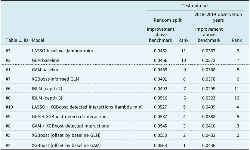
We use the ILEC VBT 2015 mortality basis as the baseline benchmark for all the models. The metric used in Table 3 is the average Poisson deviance improvement against this benchmark.
Improvement of average Poisson deviance above ILEC VBT 2015 basis on test data sets by models

Table 3. Long description
The table presents a comparison of various models based on their improvement of average Poisson deviance above the ILEC VBT 2015 basis on test data sets. It includes two main sections for test data sets: Random split and 2018-2019 observation years. Each section lists the improvement above benchmark and the corresponding rank for each model. The models compared include LASSO baseline, GLM baseline, GAM baseline, XGBoost-informed GLM, IBLM at different depths, LASSO with XGBoost detected interactions, GLM with XGBoost detected interactions, GAM with XGBoost detected interactions, and XGBoost with different offsets. Notable trends include XGBoost models generally showing higher improvements and better ranks across both test data sets.
Across both test data sets, the black-box XGBoost models were the most performant (Table 3). Amongst the three hybrid approaches being appraised, the interaction detection approach resulted in the highest improvement against the baseline benchmark. Amongst the interaction-detection-based models, the GAM method performed best both on the random split and on the 2018–2019 test data. The IBLM outperformed all the baseline models and the XGB-informed GLM, but not the interaction detection approaches, on the random split. However, on the 2018–2019 test data, the IBLM underperformed all other models.
3.2. Analysis Insight
3.2.1 Feature Importance
Feature importance rankings are broadly similar across different models. Thus, we focus on the XGBoost results shown in Figure 1. Attained age is the most important feature, consistent with its well-known exponential relationship with mortality. Face amount band is the second most important feature, ranking above smoker status, duration and sex. This may reflect the wide range of sums assured from $0–9,999 to $10 million+ in the data set. Unlike typical UK life insurance data sets, over 13% of the life years exposure is for policies in excess of $1 million.
Since the final GAM (model 8, Table 1) is the best-performing interaction-detection-based model, we use it to explain the insights from the relative importance of pairwise interaction terms (Figure 3). Compared to our CMI study that applied the same methodology (Tam & Luteijn, Reference Tam and Luteijn2025), face amount band (sum assured) features more prominently in pairwise interactions in the ILEC data set. The most important interaction is between face amount band and attained age, which ranked second in our CMI study. The interaction between duration and face amount band ranked second on the ILEC data, but 8th in the CMI study. We hypothesise that face amount band is more important in the ILEC data because of the wider range of sums assured, higher levels of income inequality in the US, and the greater variation in underwriting comprehensiveness by sum assured in the US.
Interaction importance for the final GAM (model 8).

Figure 3. Long description
The horizontal bar graph compares the coefficient of variation of relativities for different interactions in the final GAM model. The x-axis represents the coefficient of variation of relativities, ranging from 0 to 18 percent. The y-axis lists the interactions, including Attained Age x Face Amount Band, Duration x Face Amount Band, Attained Age x Duration, Attained Age x Observation Year, Attained Age x Smoker Status, Face Amount Band x Observation Year, Attained Age x Sex, Face Amount Band x Smoker Status, Duration x Observation Year, and Observation Year x Sex. The bars are colored blue and vary in length, indicating the relative importance of each interaction. The longest bars represent the highest coefficients of variation, with Attained Age x Face Amount Band and Duration x Face Amount Band showing the most significant values. All values are approximated.
3.2.2 Partial Dependency
We focus on explaining the insights from the partial dependency plots from GAM, which is the best-performing model under the interaction detection approach.
Baseline GAM
This section describes the impact of the top 4 features (Figure 4) in the baseline GAM (model 1) on mortality in the ILEC data set.
Partial dependence plots for the top 4 features in the baseline GAM.

Figure 4. Long description
The image contains four partial dependence plots. The first plot, labeled Attained Age, shows a histogram of live years exposure with a red line representing relativity on a log scale. The second plot, labeled Smoker Status, displays a bar for smokers and non-smokers with a red line for relativity. The third plot, labeled Face Amount Band, presents a histogram of live years exposure with a red line for relativity. The fourth plot, labeled Duration, shows a histogram of live years exposure with a red line for relativity. Each plot illustrates the relationship between the feature and the model’s output, highlighting how different factors influence the outcome.
For attained age, mortality is elevated between ages 20 and 30 before reaching the lowest level in the early 30s (Figure 4). This effect was also seen in our CMI analysis (Tam & Luteijn, Reference Tam and Luteijn2025) and is known as the excess mortality hump, which usually takes place between ages 15 and 30 across different countries (Remund et al., Reference Remund, Camarda and Riffe2021). This effect may be more prominent for an insured population where external causes of death, such as unintentional injuries, suicide and homicide, are more difficult to screen out through underwriting. It could also be that, at younger ages, anti-selection is more visible due to lower baseline mortality amongst younger lives in the general population.
The mortality risk of smokers is about 150% higher than that of non-smokers after controlling for other factors (Figure 4), which corroborates the regression coefficient of 2.62 for smokers (relative to non-smokers) in the baseline GLM. This excess mortality amongst smokers varies by age, as evidenced by the interaction between attained age and smoking status being the sixth-ranked interaction (Figure 3).
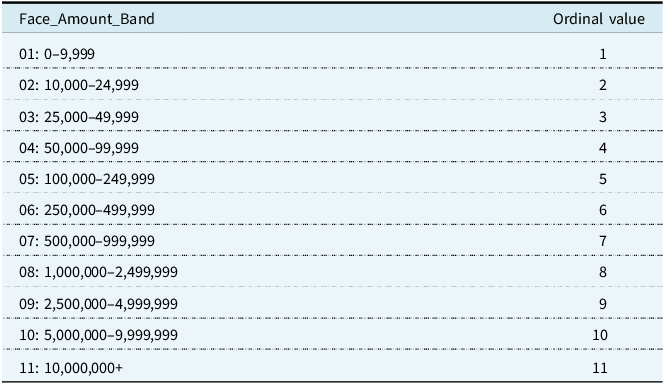
In this model, face amount band is treated as an ordinal variable and the mapping from the bands to ordinal values is shown in Table 4. Mortality decreases as the amount bands increase, with the first three bands having similarly high risk before dropping sharply for bands $100–250K and $250–500K. The sharp differential between policies below $100K (which often have weaker underwriting) and policies above $100K often leads to the exclusion of policies below $100K in ILEC experience studies (Individual Life Insurance Experience Committee of the Society of Actuaries, 2024).
Ordinal encoding of face amount bands

The partial dependence plot for duration (Figure 4) shows an extraordinarily long select shape of at least 20 years. It is conceivable that this is a product of improvements in underwriting and products over time, especially since our models did not incorporate any adjustments for issue year. In the US, products have become progressively sophisticated in relation to number of preferred classes. Since these features were outside of scope of our models, any confounding by product type including number of preferred classes will not have been adjusted for.
Final GAM with Interactions
This section describes the impact of the top interactions (Figure 5) in the final GAM (model 8) on mortality in the ILEC data set.
Top two interaction partial dependence plots for model #8.

Figure 5. Long description
The image contains two line graphs side by side. The left graph, titled ‘Attained Age x Face Amount Band,’ shows the relationship between attained age and relativity on a log scale. The x-axis represents attained age ranging from 20 to 90 years, while the y-axis represents relativity. Different colored lines represent various face amount bands: Below 100k, 100k to 250k, 250k to 500k, 500k to 1 million, and 1 million plus. The right graph, titled ‘Duration x Face Amount Band,’ illustrates the relationship between duration and relativity. The x-axis represents duration ranging from 1 to 19 years, and the y-axis represents relativity. Similar to the left graph, different colored lines represent various face amount bands. The color bar on the right indicates the face amount band corresponding to each line color. The graphs show how relativity changes with attained age and duration across different face amount bands.
The highest-ranking interaction is between face amount band and attained age (Figure 3). Mortality is especially high for the face amounts below $100K across all ages. The differential in mortality rates by face amount band is especially wide for ages 30–40, following which it converges with increasing age. From age 70 onwards, there is no meaningful mortality difference across face amount bands above $100K, but the mortality excess for policies below $100K remains elevated until age 90.
The second-ranking interaction is between face amount band and duration (Figure 3). In addition to the evidently much higher mortality for smaller face amount bands, there is a clear dichotomy between bands 1–4 (below $100K) and bands 5–11 (above). For policies below $100K, there is barely a select effect, presumably due to much lower underwriting requirements for these policies in the US. (Society of Actuaries Research Institute, 2024) For policies above $100K, full underwriting is the default, and this is reflected in the presence of a select shape. The mortality differential for face amount bands above $100K does not appear to compress at higher durations.
4. Appraisal of the Hybrid Approaches
We demonstrated three innovative approaches for using gradient boosting to enhance traditional additive models in the context of mortality modelling. Additionally, we tested variations of the interaction detection approach using additive models (i.e. GLM, LASSO and GAM) as the final output.
4.1. Model Performance
All three hybrid approaches (models 6–10) outperformed the baseline models (models 1–3), but underperformed the black-box models (models 4 and 5). Amongst the three hybrid approaches, the interaction detection approach was the most performant across both test data sets (Table 3). The performance of the XGBoost-informed GLM and the interaction detection approach depends on the modeller’s ability to distinguish true signal from noise, perform feature engineering, and craft an effective regression formula. This reliance on modeller expertise is especially acute for GLM and LASSO, as GAM auto-calibrates nonlinearities.
IBLM has not previously been applied to life and health insurance data sets, and it is conceivable that for such data the initial GLM will leave a lot of signal on the table for the booster model to pick up. For example, in life and health the relationship between attained age and mortality is exponential, as can be seen in both Figures 2 and 4. A single linear term in the initial GLM is insufficient to capture its complexity. The performance ranking of IBLM dropped for the out-of-time test data. This is hypothesised to be due to the inability of the internal booster model to extrapolate an observation year effect.
Amongst the interaction detection approaches, GAM outperforms GLM and LASSO on both the random split and the 2018–2019 test data when including interaction terms. This could be due to GAM having more flexible curve fitting, while controlling for overfitting via both L2 regularisation and a roughness penalty on numerical features.
In the random split, the final GAM attains a deviance improvement 16% higher than the baseline GAM. This is about 80% of the improvement attained by the corresponding XGBoost. In the 2018–2019 test data, the final GAM attains 11% improvement – about 62% of the corresponding XGBoost improvement. With sufficient lives exposure, as in the ILEC data set, there is a trade-off between transparency and accuracy. However, health & care insurers do not usually have sufficient exposure or achieve full claim credibility at the level of customer granularity they require. Under these circumstances, underwriting knowledge and actuarial judgement are key to determining whether risk models capture genuine trends. Having transparent models enables scrutiny and ensures they do not overfit to training data.
4.2. Modeller Control
The three approaches are subject to varying levels of automation, with the IBLM being the most automated, and the XGB-informed GLM the least automated. The interaction detection approach and XGB-informed GLM offer high levels of modeller control since, in both cases, the XGB is used as a diagnostic tool rather than the final predictive engine. The modeller retains full control over how variables are engineered and what interactions are incorporated in the model. This does come at the cost of increased fragility, as predictive performance is more dependent on the expertise and domain knowledge of the modeller.
The IBLM approach automatically detects nonlinearities and interactions and incorporates these back into the final model predictions through SHAP-derived beta adjustments. This automation reduces manual feature engineering and may improve predictive performance. Unlike the other two approaches, all possible variable interactions are considered by default. The IBLM booster can be controlled by specifying interaction and monotonic constraints and tree depth, offering a degree of modeller control. Contrary to the two other approaches (which require a regression formula), IBLM offers strong out-of-the-box performance. Due to the split-based nature of XGB, the IBLM approach does not naturally produce smooth relationships between continuous predictors and outcomes, which may impair predictive performance, especially where high learning rates have been selected.
All three approaches offer meaningful levels of modeller control. The main difference is that the interaction detection approach and the XGBoost-informed GLM allow the modeller to directly specify the functional form of predictor-outcome relationships. For example, logarithmic transformations can enforce proportional effects of sum assured on the outcome, while trigonometric functions enforce a seasonal effect. These explicit levels of control allow actuaries to embed domain knowledge into their models and support extrapolation and interpretation (Luteijn et al., Reference Luteijn, Tam, Denis, Fan, Minhas, Puthanveedu and Takyi2026). The split-based nature of XGBoost does not allow for enforcing these types of effects.
4.3. Transparency and Governance Readiness
Although TAS 100 does not define a transparency requirement, compliance with principle 5 (models) and principle 7 (communication) requires a level of understanding and explainability that means that transparency is, in effect, mandated (Financial Reporting Council, 2023). Lack of transparency could result in biases against certain customer segments that violate regulatory requirements or produce model outputs changes that cannot be adequately justified to internal stakeholders (e.g. risk managers) and external ones (e.g. customers).
The interaction detection approach and the XGB-informed GLM result in final additive models, including explicitly specified main effects and variable interactions, each with fixed regression coefficients. Although regression coefficients of polynomials can be less intuitive to interpret, individual effects and interactions can be visualised explicitly and scrutinised using domain knowledge, supporting validation and governance review.
In contrast, the final output of IBLM is a GLM model, augmented by a set of SHAP-derived beta adjustments, reflecting the contribution of the internal XGB booster model on the linear predictor scale. These beta-adjustments can be highly observation-specific, subject to the tree-depth of the booster model. While in our study tree depths of 2 and 3 were modelled, restricting the complexity of the beta adjustments, deeper trees can capture higher-order variable interactions, materially reducing interpretability while potentially boosting predictive accuracy. This reduced interpretability for deep IBLM booster models can have negative implications for governance and transparency. By contrast, the IBLM approach will produce consistent results across different modellers and therefore is not exposed to governance risk if interaction selection or feature engineering rationale is poorly documented.
4.4. Applicability to Actuarial Modelling Tasks
The three hybrid approaches assessed aim to improve the ability of additive models to capture nonlinearities and interactions at the structural level. Therefore, the contribution of the paper is methodological, rather than outcome-specific.
Although the data set analysed contains mortality events, the underlying modelling setup is representative of a broader set of actuarial modelling tasks. Mortality, morbidity, income protection, lapse and fraud detection all involve modelling of rare event counts per unit of exposure. These tasks involve strong nonlinearities and interactions across biometric (e.g. age, sex, smoking), insurance (e.g. sales channel, underwriter loading) and temporal (e.g. duration, calendar year, issue year) features. Residual boosting, interaction detection and SHAP-informed feature engineering are designed to identify and incorporate such nonlinearities and interactions in the linear predictor, independent of whether the underlying outcome represents mortality, morbidity or lapses.
4.5. Next Steps
This paper focused on hybrid modelling approaches that produce a final additive model closely aligned with established GLM-centric actuarial workflows. Therefore, various alternative explainable ML models that depart more substantially from standard actuarial workflows were not appraised. This scoping choice was made to preserve comparability across approaches, limit computational and tuning complexity, and maintain a consistent governance and documentation framework.
A natural extension would be to appraise fully automated explainable supervised techniques, including explainable boosting machines (Nori et al., Reference Nori, Jenkins, Koch and Caruana2019) and neural network models with connectivity restricted to just univariate and pairwise interactions, for example NODE-GAM (Chang et al., Reference Chang, Caruana and Goldenberg2022). These models are further removed from traditional actuarial workflows. Comparison against the hybrid approaches would focus on the trade-off between prediction accuracy and model complexity and governance. Another more natural extension could be to include approaches leveraging ML to engineer features for downstream additive models (Dai, Reference Dai2018; Henckaerts et al., Reference Henckaerts, Antonio, Clijsters and Verbelen2018; Maillart, Reference Maillart2021).
Beyond model classes, future work could extend the appraisal to morbidity, income protection, and lapse or fraud detection tasks. Critical illness claims are a particular promising area for application of hybrid approaches since public health interventions such as HPV vaccination and breast cancer screening cause strong nonlinearities in claims incidence by age and birth cohort. Additionally, there is higher risk of anti-selection (compared to mortality claims), which may manifest itself as interactions between sum assured, issue age and/or sales channel. However, health and care data sets may contain additional complexities including partial claims, severity ratings and heterogeneous outcome definitions, which may not translate to mortality data sets.
Finally, there is scope to enhance the hybrid approaches themselves. The interaction detection approach could be enhanced by use of diagnostics such as SHAP dependence plots to identify potential poorly captured nonlinearities in the baseline. The IBLM baseline model could be extended to allow bespoke regression formulae into the IBLM baseline model and hyperparameter tuning of the XGBoost model, trading training time for improved predictive performance.
5. Conclusion
To our knowledge, this is the first actuarial study to systematically appraise hybrid GLM–ML approaches along governance-relevant dimensions rather than predictive accuracy alone, using a shared data set and evaluation protocol. Across the appraisal dimensions considered in this paper, no single modelling approach dominates in all respects. Instead, the three hybrid approaches occupy different points along the trade-off between automation, modeller control, and transparency. The fully automated IBLM approach offers strong out-of-the-box performance with minimal manual intervention. Therefore, IBLM is well-suited for time-constrained modellers and modellers with little domain knowledge to hand-craft regression formulae.
The more manual XGBoost-informed GLM and interaction detection approaches allow experienced modellers to incorporate domain knowledge directly into the modelling process, particularly when capturing nonlinearities and interaction effects. These approaches retain an explicit additive structure and naturally support extrapolation in continuous features, which can be advantageous in actuarial applications requiring forward-looking judgement.
In conclusion, our findings suggest that hybrid modelling frameworks provide a flexible and practical pathway for leveraging state-of-the-art black box models into actuarial practice. For actuaries seeking to improve on purely GLM-based methods, without compromising on transparency, these hybrid approaches represent a pragmatic middle ground.
Acknowledgements
We would like to thank Ramen Marudamuthu for his valuable input and for providing insights from his perspective as a pensions actuary.






 Open access

