


1. Introduction
One of the greatest challenges in researching covert networks is collecting valid and relevant covert network data. The secretive aspects that are a defining feature of covert networks present some notable difficulties in implementing conventional data collection methods (e.g., surveys, interviews) as the covert actors themselves strive to avoid detection and remain hidden (Morselli, Reference Morselli2009; Oliver et al., Reference Oliver, Crossley, Edwards, Koskinen and Covert2014). Consequently, covert network researchers are at the mercy of whatever data regarding the network that they can access.
Covert network researchers use indirectly observed data such as wiretap records, publicly available information databases, and police investigation reports to construct a covert network for analysis (Coutinho et al., Reference Coutinho, Diviák, Bright and Koskinen2020; Ficara et al., Reference Ficara, Curreri, Fiumara, De Meo and Liotta2022; Krebs, Reference Krebs2002). To clarify, “indirect” data collection is when research is conducted with data that were recorded for different (i.e., non-research) purposes. Evidently, the researcher is unable to filter data to carefully address the relevant theoretical constructs in their research question. Indirectly observed data are vulnerable to observational biases because these data are often collected for non-research purposes, thus contributing to the issue of missing data in covert networks.
The issues surrounding missing data have been discussed numerous times in covert network research, particularly involving the use of indirect observations of the covert network, (Bright et al., Reference Bright, Brewer and Morselli2021; Calderoni et al., Reference Calderoni, Catanese, De Meo, Ficara and Fiumara2020; Diviák, Reference Diviák2020). In discussions and simulations exploring missing covert network data, the mechanisms that cause missing data are often implicit. That is, it is rare to clarify an explicit statistical model to systematically represent the probabilities of missing tie variables. Importantly, the convention for investigating missing network data is with missing tie variables, where missing values can be either a tie or null tie. For a further discussion of the issue of missing data in covert networks, see Januar et al. (Reference Januar, Colin Gallagher and Koskinen2026). Here, instead of examining the consequences of specific sources of missing data, we investigate empirical biases in the process of observing a covert network. We also provide a few novel implementations of network statistical models to represent a biased sampling process.
Specifically, the empirical biases we examine in this paper are relevant to the practice of collecting and constructing covert networks. We argue that the process of constructing covert networks is often more appropriately described as an edge sampling process instead of tie variable sampling. This reflects the empirical bias to gather information for, but not against, the presence of a tie. Even in the case of non-covert networks, name generators ask respondents for people they are tied to, not whom they are not tied to. Additionally, we evaluate dependence between sampled edges. Dependence in this case can be attributed to observational biases that can be encountered when information about the network is not easily accessible.
As a consequence of limited sources of information, we posit that more accessible sources are scrutinized which can result in a biased perspective when constructing the covert network. Specifically, we define what might be termed a person of interest bias (POI bias) and operationalize it using the contagion parameter in an auto-logistic actor attribute model (ALAAM; Daraganova and Robins, Reference Daraganova and Robins2013; Robins et al., Reference Robins, Pattison and Elliott2001) on the line graph representing the functional dependencies between sampled edges. The POI bias can represent a spotlight effect (Smith and Papachristos, Reference Smith and Papachristos2016), where focus on a certain actors’ activities may lead the investigator to focus predominantly on their activities and comparatively less focus on other actors. Practical applications of network analysis for informing target prioritization may similarly be biased if the actors’ observed position in the network is not reflective of their relative importance within the network (Hashimi and Bouchard, Reference Hashimi and Bouchard2017).
The manuscript begins with a review of the methodology of sampling covert networks and distinguishes tie variable sampling from edge sampling. Afterwards, the properties of independent edge sampling are explored. We argue that independent edge sampling is unrealistic for sampled social networks. In order to represent more realistic sampling mechanisms, we introduce dependence assumptions in edge sampling processes. Specifically, we use the line graph of the sampled network alongside the ALAAM to systematically capture biased sampling processes. Lastly, we apply the ALAAM on various population networks and find that biased sampling mechanisms result in a sampled structured network regardless of the social structures in the population network.
2. Covert network sampling
Rich and informative data are required for the investigation of covert networks, however the secretive nature of covert networks presents many difficulties in studying the phenomena. These difficulties have many different facets, ranging from the difficulties in directly observing members of the covert network to various potential biases as researchers attempt to construct the covert network from whatever data are available. In the latter case, Bright et al. (Reference Bright, Brewer and Morselli2021) describe different criminal justice records that researchers have used to study criminal networks. These include investigative reports, law enforcement reports, offender databases, prosecution and court files, departmental inquiries, and multiple other sources. These data sources arise from documentation processes not designed for research purposes. As described in Bouchard (Reference Bouchard2021), police data alone may not be sufficient to understand gang networks. Auxiliary records (i.e., administrative records, prison logs) can enrich the context by which police data are observed, giving the researcher a clearer understanding of the network.
Putting aside the difficulties of accessing the data in the first place, when we evaluate the statistical implications of using data representing indirect observation of the network, we inevitably run into the possibility of biases in the data. Morselli (Reference Morselli2009) note that data obtained through an investigation may be biased by the proceedings of the investigation and subsequent judicial proceedings. For example, high-profile and active individuals from the network are more likely to be surveilled and convicted than peripheral members of the network (Malm and Bichler, Reference Malm and Bichler2013).
Another example is the use of wiretap data (Berlusconi, Reference Berlusconi2013; Campana and Varese, Reference Campana and Varese2012). Wiretap transcripts are selected depending on the relevance of its content during an investigation, thus introducing the possibility of bias through the choice of certain transcripts. However, we would also like to note two particular biases that have not been addressed that have important statistical implications, (a) there is a tendency to define edges, but not null ties, and (b) there is dependence between sampled edges.
3. Empirical covert network sampling biases
When confirming the existence of ties, absence of evidence is not evidence of absence.Footnote 1 A few examples of the tendency to identify ties instead of null ties can be seen in the examples described above. Criminal justice records describe observations that have been recorded. Law enforcement organizations would want to record as much relevant information about their investigation. A researcher can access these records and infer potential social relationships involved in the execution of the action. In doing so, the researcher elaborates which relational elements can support the existence of a tie, whereas the null tie is simply defined as the inability to fit the tie definition criteria. There does not seem to be any criteria to confirm the non-existence of a particular relationship outside of the inability to define a relationship.
A potential source of this bias can be couched in terms of a cognitive bias lens. A relevant effect is a feature positivity effect where presence is more salient than absence, despite both outcomes being informative (Meterko and Cooper, Reference Meterko and Cooper2022). For example, Eerland et al. (Reference Eerland, Post, Rassin, Bouwmeester and Zwaan2012) found that the presence of fingerprints as opposed to a lack of fingerprints is more readily remembered, opposed to a lack of fingerprints, and used to make decisions about a criminal case. This relates back to the spotlight effect discussed above. For example, if police investigators focus primarily on identifying ties for known potential suspects, they are more likely to establish potential ties between the known suspects while missing any relevant unknown individuals. By focusing on identifying ties, as discussed below, it may also make it difficult to identify possible divisions or factions between the social network.
Despite being less salient, identifying null ties still has important theoretical implications when considering subgroup formation in social networks. Breiger (Reference Breiger1974) describes an example of where the confirmed presence of no relationship between nodes in the network indicates how subgroups within the graph are defined. In the example, Breiger investigates the attendance of women at multiple social events and describes it as a bipartite network. He then states that the events where there are no overlapping attendees with all the other events separates subgroups of women within the community. Additionally, White et al. (Reference White, Boorman and Breiger1976) describes how the indicator of structurally equivalent members of a network in a blockmodel are primarily defined by the absence of ties between sets of structurally equivalent individuals (for clarification on the concept of structural equivalence, see Lorrain and White (Reference Lorrain and White1971)). The broader network literature has acknowledged the importance of defining null ties to identify meaningful subgroups within a network, but there is a lack of discourse on the practicalities of confirming null ties.
Sampling null ties may, in theory, be advantageous for identifying social structure. However, such an approach faces a major flaw in practice. A null tie is not confirmed simply because the collected information does not imply a tie. An example for evidence of null ties can be seen in Zachary (Reference Zachary1977). The article emphasized bottlenecks of information flow to represent a division between factions of a club. The division in Zachary (Reference Zachary1977) was identified when there were no interactions between the two prominent figures in contexts outside of club activity. Therefore, the sampling of null ties may be especially useful when identifying divisions between different groups. Future explorations into sources of covert network data representing information flow for determining internal divisions may be insightful to illuminate the definition of null ties.
We may never be able to identify all the individuals attending a particular event or collaborating in an illicit manner. Investigators would need to identify individuals who belong to the covert network and confirm the absence of social relationships between them, which would take substantial resources. It is largely unfeasible as investigations often operate with a constraint on the quantity of resources used as well as other possible regulatory constraints (e.g., judicial proceedings). Therefore, we argue that there is a tendency to define edges over null ties. Januar et al. (Reference Januar, Colin Gallagher and Koskinen2026) demonstrates how systematic observational biases can be represented in effects in a model for the missing data. In this work, we similarly represent plausible sampling biases using effects in a statistical model.
The second bias we address is the dependence between sampled edges. In this case, we argue against the statistical independence of sampled information. We motivate this bias through the descriptions of sampling procedures in the discipline. As described in Figure 1, researchers narrow down criteria to decide how an edge is defined from the wide variety of information about the network. Scholars have described the overall process to reflect a snowball-like or purposive sampling process instead of random sampling (Bright et al., Reference Bright, Brewer and Morselli2021), as random sampling is not practical when dealing with network data (Robins, Reference Robins2015). To clarify, purposive sampling is a non-probability sampling method to select individuals who fit a particular set of criteria within a population.
Illustration of a non-independent sampling process as wiretap records are selectively chosen. Adapted from Berlusconi (Reference Berlusconi2013).

Snowball sampling can refer to both a non-probability convenience sampling method and a probability sampling method (Handcock and Gile, Reference Handcock and Gile2011). To clarify the probability sampling method usage defined in Goodman (Reference Goodman1961), it states that for a given (randomly sampled) seed set, all of the seed nodes’ alters are sampled. These sampled alters are the first wave. Further details on technical aspects of snowball sampling as a probability sampling method can be found in Frank (Reference Frank1977) and Frank and Snijders (Reference Frank and Snijders1994). Subsequent waves sample all of the previous waves’ alters. Importantly, snowball sampling assumes that (a) all of a sampled node’s alters are sampled, and (b) snowball sampling is a sample of nodes and the edges are incidentally sampled.
We argue the process of sampling covert networks is snowball-like. That is, it is similar to (probabilistic) snowball sampling, but is not exactly accurate. The assumption that all of a sampled node’s alters are sampled is rather strict. In practice, especially when dealing with covert network information, it is difficult to sample all of a node’s ties and the consequences of these snowball-like procedures are unclear.
These biases can be encountered across multiple layers of observation. Law enforcement personnel may be selective during the collection of evidence when building a case. Future work may explore the effects of multiple observers of the covert network and the incurred consequences when conducting network analysis. The current manuscript aims to describe the existence of these biased edge sampling processes and a methodology to explore them.
The sampling of edges are unlikely to be truly independent as information about sampled edges may inform the sampling of subsequent edges. For example, if there were a theoretical “person of interest,” sampling edges involving this person may make it more likely to sample subsequent edges involving this person, because these subsequent edges involve the same person. Therefore in this manuscript, we explore the modeling of covert network discovery as a snowball-like edge sampling process. Specifically, we use the line graph of the network with an ALAAM to systematically define biased edge sampling processes.
4. Notation and definitions
We introduce some notation to distinguish the typical evaluation of dyads, or tie variables, and the process of sampling edges. We use the adjacency matrix $\mathbf{X}$
to represent an arbitrary undirected graph
$\mathbf{X}$
to represent an arbitrary undirected graph $G = G(V,E)$
with
$G = G(V,E)$
with $N = |V|$
vertices in vertex set
$N = |V|$
vertices in vertex set $V$
and
$V$
and $U = |E|$
edges in edge set
$U = |E|$
edges in edge set $E$
. The tie variables in the adjacency matrix
$E$
. The tie variables in the adjacency matrix $x_{ij}$
are defined as
$x_{ij}$
are defined as
 \begin{align} x_{ij} = \begin{cases} 0 & \text{if } {ij} \notin E \\ 1 & \text{if } {ij} \in E \\ \end{cases}. \end{align}
We define a null tie as the non-existence of a relationship, usually indicated by a 0 in an adjacency matrix $\mathbf{X}$
.
$\mathbf{X}$
.
In previous literature exploring network sampling designs, a sampling indicator matrix $\mathbf{S}$
is defined to indicate whether the corresponding tie variable is sampled (Frank, Reference Frank1977; Gile and Handcock, Reference Gile and Handcock2006; Handcock and Gile, Reference Handcock and Gile2010). In the current manuscript, we restrict the sampling indicator matrix
$\mathbf{S}$
is defined to indicate whether the corresponding tie variable is sampled (Frank, Reference Frank1977; Gile and Handcock, Reference Gile and Handcock2006; Handcock and Gile, Reference Handcock and Gile2010). In the current manuscript, we restrict the sampling indicator matrix $\mathbf{S}$
to be
$\mathbf{S}$
to be
 \begin{align} s_{ij} = \begin{cases} 0 & \text{if } x_{ij} \text{ is not sampled or $x_{ij} = 0$}\\ 1 & \text{if } x_{ij} \text{ is sampled} \end{cases}. \end{align}
To clarify, we restrict the sampling indicator to only edges and null ties, by definition, are not sampled. It follows that the observed adjacency matrix represents a graph $G(V, E^*)$
where
$G(V, E^*)$
where $E^*$
is a random subset of
$E^*$
is a random subset of $E$
,
$E$
, $E^{\ast } \subseteq E$
. The observed adjacency matrix can be defined as the element-wise product of the sampling indicator and the adjacency matrix,
$E^{\ast } \subseteq E$
. The observed adjacency matrix can be defined as the element-wise product of the sampling indicator and the adjacency matrix, $\mathbf{X}^* = \mathbf{X} \odot \mathbf{S}$
. It follows that the tie variables of the observed adjacency matrix
$\mathbf{X}^* = \mathbf{X} \odot \mathbf{S}$
. It follows that the tie variables of the observed adjacency matrix $\mathbf{X}^*$
are defined as
$\mathbf{X}^*$
are defined as
 \begin{align} x^*_{ij} = \begin{cases} 1 & \text{if } s_{ij} = 1 \\ NA & \text{if } s_{ij} = 0 \end{cases}. \end{align}
As we restrict sampling to only edges, any unsampled variable ( $s_{ij} = 0$
) is by definition missing (
$s_{ij} = 0$
) is by definition missing ( $NA$
). A common practice is to assume unsampled edges are null ties. However, this practice is clearly erroneous for edges and the resulting network can often be biased depending on the quantity of missing tie variables (Huisman, Reference Huisman2014). We define an edge sampling process as the process where the observed edges
$NA$
). A common practice is to assume unsampled edges are null ties. However, this practice is clearly erroneous for edges and the resulting network can often be biased depending on the quantity of missing tie variables (Huisman, Reference Huisman2014). We define an edge sampling process as the process where the observed edges $e \in E^*$
are sampled with some probability
$e \in E^*$
are sampled with some probability $p$
. It follows that any tie-variable that is not an edge in
$p$
. It follows that any tie-variable that is not an edge in $E$
is not sampled,
$E$
is not sampled,
 \begin{align} {\Pr}(S_e = 0 | e \notin E) = 1, \end{align}
and that any edge that was sampled in the observed graph is also in the true edge set,
 \begin{align} {\Pr}{(e \in E| e \in E^*)} = 1. \end{align}
The probability of sampling an edge $p$
can be homogeneous if all the edges are equally as likely to be sampled or heterogeneous if there are systematic differences in the probability of certain edges being sampled. We further elaborate edge sampling processes below.
$p$
can be homogeneous if all the edges are equally as likely to be sampled or heterogeneous if there are systematic differences in the probability of certain edges being sampled. We further elaborate edge sampling processes below.
5. Edge sampling
There are few works that have explored the properties of edge sampling (Bollobás, Reference Bollobás2001; Frank, Reference Frank1971). The computer science literature has explored “edge sampling” as algorithms to reduce network size or generate sparse graphs (Le, Reference Le2021; Su et al., Reference Su, Liu, Kurths and Meyerhenke2024). We distinguish our definition of edge sampling in this manuscript to explicitly refer to statistical models for sampling social networks. In contrast to missingness models in general (Rubin, Reference Rubin1975) or applied to network data (Januar et al., Reference Januar, Colin Gallagher and Koskinen2026), the following edge sampling models are restricted to tie variables that are edges ( $x_{ij}$
= 1).
$x_{ij}$
= 1).
An edge sampling model describes the probabilities of selecting (sampling) certain edges. For example, in an edge sampling process where each edge was sampled independently with a uniform probability $p$
, the model can be described as
$p$
, the model can be described as
 \begin{align} {\Pr}(S_{ij} = 1 | {ij} \in E) = p. \end{align}
As each edge would be sampled according to a Bernoulli trial with probability $p$
, it follows that the number of sampled edges follow a Binomial distribution,
$p$
, it follows that the number of sampled edges follow a Binomial distribution,
 \begin{align} \sum _i S_{ij} \sim Bin \left (\sum _i X_{ij}, p \right ). \end{align}
An example of an independent edge sampling process are stochastic contact graphs described in Frank (Reference Frank1971). Stochastic contact graphs assume that the edges are sampled independently with a uniform probability $p$
. In this manuscript we only consider stochastic contact graphs of simple graphs (i.e., no multiple edges or loops).
$p$
. In this manuscript we only consider stochastic contact graphs of simple graphs (i.e., no multiple edges or loops).
For stochastic contact graphs, limited results are available for realistic networks. In this case, the undirected population graph is represented by a symmetric adjacency matrix $\mathbf{X}$
and the stochastic contact graph (and sample graph) is represented by the symmetric adjacency matrix
$\mathbf{X}$
and the stochastic contact graph (and sample graph) is represented by the symmetric adjacency matrix $\mathbf{X}^*$
where
$\mathbf{X}^*$
where $x^*_{ij} = 1$
if
$x^*_{ij} = 1$
if $x_{ij} = 1$
, sampled with independent Bernoulli probability
$x_{ij} = 1$
, sampled with independent Bernoulli probability $(p)$
for
$(p)$
for $i \lt j$
, otherwise
$i \lt j$
, otherwise $x^*_{ij} = 0$
.
$x^*_{ij} = 0$
.
For the local degrees of two different nodes $i$
and
$i$
and $j$
in an undirected graph,
$j$
in an undirected graph, $x_{i+}$
and
$x_{i+}$
and $x_{j+}$
, any sampled node
$x_{j+}$
, any sampled node $i$
has a degree of
$i$
has a degree of $x^*_{i+} \thicksim Bin(x_{i+},p)$
. From these results, Frank (Reference Frank1971) derived the joint distribution of the degrees of two different nodes
$x^*_{i+} \thicksim Bin(x_{i+},p)$
. From these results, Frank (Reference Frank1971) derived the joint distribution of the degrees of two different nodes $i$
and
$i$
and $j$
to be
$j$
to be
 \begin{align} Pr(x^*_{i+} & = a, x^*_{j+} = b) = (1 - x_{ij}) P(a, x_{i+})P(b, x_{j+}) \nonumber \\& \quad + x_{ij}[(1-p) P(a,x_{i+} -1)P(b, x_{j+}-1) + pP(a-1, x_{i+}-1)P(b-1, x_{j+}-1)] \end{align}
for all $i \neq j$
and
$i \neq j$
and $P(a, A)$
defined as
$P(a, A)$
defined as
 \begin{align} P(a, A) = \left(\begin{array}{c}A \\ a\end{array}\right) p^a (1-p)^{A - a}, \end{align}
for $a$
and
$a$
and $A = 0, 1, \ldots , N-1$
, i.e., the pmf for a
$A = 0, 1, \ldots , N-1$
, i.e., the pmf for a $Bin(A,p)$
evaluated in
$Bin(A,p)$
evaluated in $a$
. To briefly summarize the joint distribution, it consists of two parts. The case where
$a$
. To briefly summarize the joint distribution, it consists of two parts. The case where $x_{ij} = 0$
, which means that the nodes already had the target degrees and the case where
$x_{ij} = 0$
, which means that the nodes already had the target degrees and the case where $x_{ij} = 1$
, which depends on the sampling probability
$x_{ij} = 1$
, which depends on the sampling probability $p$
.
$p$
.
The joint distribution is used to determine the expected degree frequencies (i.e., the degree distribution) $f_{x^*}(a)$
for
$f_{x^*}(a)$
for $a = 0, 1, \ldots , N$
. Explicitly, this expectation is
$a = 0, 1, \ldots , N$
. Explicitly, this expectation is
 \begin{align} \mathbb{E} \left [ f_{x^*}(a) \right ]= \sum _{i = 1}^N P(a, x_{i+}) = \sum _{A = 0}^N P(a, A)f_x(A). \end{align}
Variances, covariances, and an unbiased estimator can be derived for this frequency. For specific details, see Frank (Reference Frank1971).
Frank (Reference Frank1971) produces some interesting additional results using stochastic contact graphs, including the estimation of cliques (i.e., complete subgraphs) of varying sizes. For example, this allows for the estimation of the number of triangles for a given node size and sampling probability, which can be useful for inspecting the connectivity of the sampled graph. However, these results require the population graph to be complete, or that every node is connected to every other node, something that does not apply in our case.
In a similar vein, Bollobás (Reference Bollobás2001) also describes an edge sampling process in his definition of reliable networks, however his results hold in the limit as the number of nodes in the graph go to infinity and assume the population graph to be connected. We consider the assumptions for reliable graphs to also be inapplicable for social networks in general because assuming social networks to be fully connected is unrealistic.
For practical applications of stochastic contact graphs, we generalize an example from the original chapter in Frank (Reference Frank1971). Consider an undirected population graph with $N$
covert actors where each edge connects two actors in a co-conspiratorial sense (e.g., “with whom do you commit secretive and potentially illegal activities?,” had the network been elicited using a name generator for covert actors). The population graph’s local degree
$N$
covert actors where each edge connects two actors in a co-conspiratorial sense (e.g., “with whom do you commit secretive and potentially illegal activities?,” had the network been elicited using a name generator for covert actors). The population graph’s local degree $x_{i+}$
is equal to the number of co-conspiracy ties for the
$x_{i+}$
is equal to the number of co-conspiracy ties for the $i$
-th covert actor. The number of actors with exactly
$i$
-th covert actor. The number of actors with exactly $A$
co-conspiracy ties equals
$A$
co-conspiracy ties equals $f_x (A)$
. We then expect that the
$f_x (A)$
. We then expect that the $i$
-th covert actor will be sampled
$i$
-th covert actor will be sampled $\mathbb{E}( x^*_{i+})$
times (i.e., average sample degree). The probability that each actor is sampled at least once equals
$\mathbb{E}( x^*_{i+})$
times (i.e., average sample degree). The probability that each actor is sampled at least once equals
 \begin{align} P(x^*_{i+} \gt 0 \text{ for } i = 1, 2, \ldots , N) = P(f_{x^*}(0) = 0), \end{align}
and the number of actors which are expected to be sampled more than once equals
 \begin{align} \mathbb{E} \left [ \sum _{r = 2}^N f_{x^*} (r) \right ] = N - \mathbb{E} \left [f_{x^*} (0)\right ] - \mathbb{E} \left [ f_{x^*} (1)\right ]. \end{align}
Overall, stochastic contact graphs gives us a framework to estimate some informative graph properties. These include the probability of the graph being connected and the expected number of isolates and cliques. While not described in this summary, stochastic contact graphs can be conditioned on the total number of edges in the graph and are applicable to both undirected and directed networks.
However, even these limited results for the estimators and general framework rely on the independence of sampled edges. A known node size $N$
is also vital for the estimators and the Bernoulli sampling probability
$N$
is also vital for the estimators and the Bernoulli sampling probability $p$
is also required. If these conditions were met (i.e., edges are sampled independently, a plausible value for the number of nodes, and some plausible value for the sampling probability), we can derive some useful properties of an unknown population graph from the specified sampling process.
$p$
is also required. If these conditions were met (i.e., edges are sampled independently, a plausible value for the number of nodes, and some plausible value for the sampling probability), we can derive some useful properties of an unknown population graph from the specified sampling process.
One last straightforward property for sampled graphs is that functions that are weakly monotone increasing in edge addition (e.g., degree, counts of triangles) will be smaller (or equal) in sampled graph. For example, for the number of triangles $t(\mathbf{X})$
,
$t(\mathbf{X})$
,
 \begin{align} t(\mathbf{X}) = \sum _{i\lt j\lt k}x_{ij}x_{ik}x_{jk}, \end{align}
the number of triangles in the sampled graph $\mathbf{X}^*$
will be smaller unless all edges in E are sampled. This finding is apparent as the edge set of the sampled graph,
$\mathbf{X}^*$
will be smaller unless all edges in E are sampled. This finding is apparent as the edge set of the sampled graph, $E^*$
, is by definition a random subset of
$E^*$
, is by definition a random subset of $E, E^* \subseteq E$
. Therefore, the number of triangles for the sampled graph will be less than or equal to the true number of triangles,
$E, E^* \subseteq E$
. Therefore, the number of triangles for the sampled graph will be less than or equal to the true number of triangles,
 \begin{align} t(\mathbf{X}^*) \leq t(\mathbf{X}). \end{align}
A similar property can be described for the connectivity of a graph. For example, if $w_{ij}=(e_1,\ldots ,e_r)$
is a path with vertex sequence
$w_{ij}=(e_1,\ldots ,e_r)$
is a path with vertex sequence $v=(v_1,\ldots ,v_r)$
, where
$v=(v_1,\ldots ,v_r)$
, where $v_1=i$
and
$v_1=i$
and $v_r=j$
, let us first define the shortest path (i.e., geodesic distance) between any two vertices,
$v_r=j$
, let us first define the shortest path (i.e., geodesic distance) between any two vertices,
 \begin{align} sp(i,j) = \min |w_{ij} |, \end{align}
where $|w_{ij} |$
is the length of the path
$|w_{ij} |$
is the length of the path $w_{ij}$
(i.e., the number of edges) from vertex
$w_{ij}$
(i.e., the number of edges) from vertex $i$
to
$i$
to $j$
. The distance between nodes that are not reachable from each other being conventionally set to infinite. The diameter of the graph is the maximum shortest path of the graph,
$j$
. The distance between nodes that are not reachable from each other being conventionally set to infinite. The diameter of the graph is the maximum shortest path of the graph,
 \begin{align} diam(\mathbf{X}) = \max _{i,j \in V} sp(i,j). \end{align}
As a subset of the edges are sampled, the diameter increases,
 \begin{align} diam(\mathbf{X}^*) \geq diam(\mathbf{X}). \end{align}
This is evident as connected components of the graph are less dense due to the subset of sampled edges $E^*$
, thus increasing the maximum path lengths. The property also holds for disconnected components as the distance between two disconnected vertices is conventionally defined as infinite. In the following sections, we describe our proposed approach to relax the independence assumption for edge sampling processes and use simulations to inspect sampled graph distributions.
$E^*$
, thus increasing the maximum path lengths. The property also holds for disconnected components as the distance between two disconnected vertices is conventionally defined as infinite. In the following sections, we describe our proposed approach to relax the independence assumption for edge sampling processes and use simulations to inspect sampled graph distributions.
6. Relaxing independence
In order to, eventually, relax the independence assumption for an edge sampling process, we need to represent the sample in a way that respects how ties are related through nodes. We do this using the graph’s line graph (Figure 2).
A sampled graph and its line graph. Blue solid edges are sampled while orange dashed edges are missing.
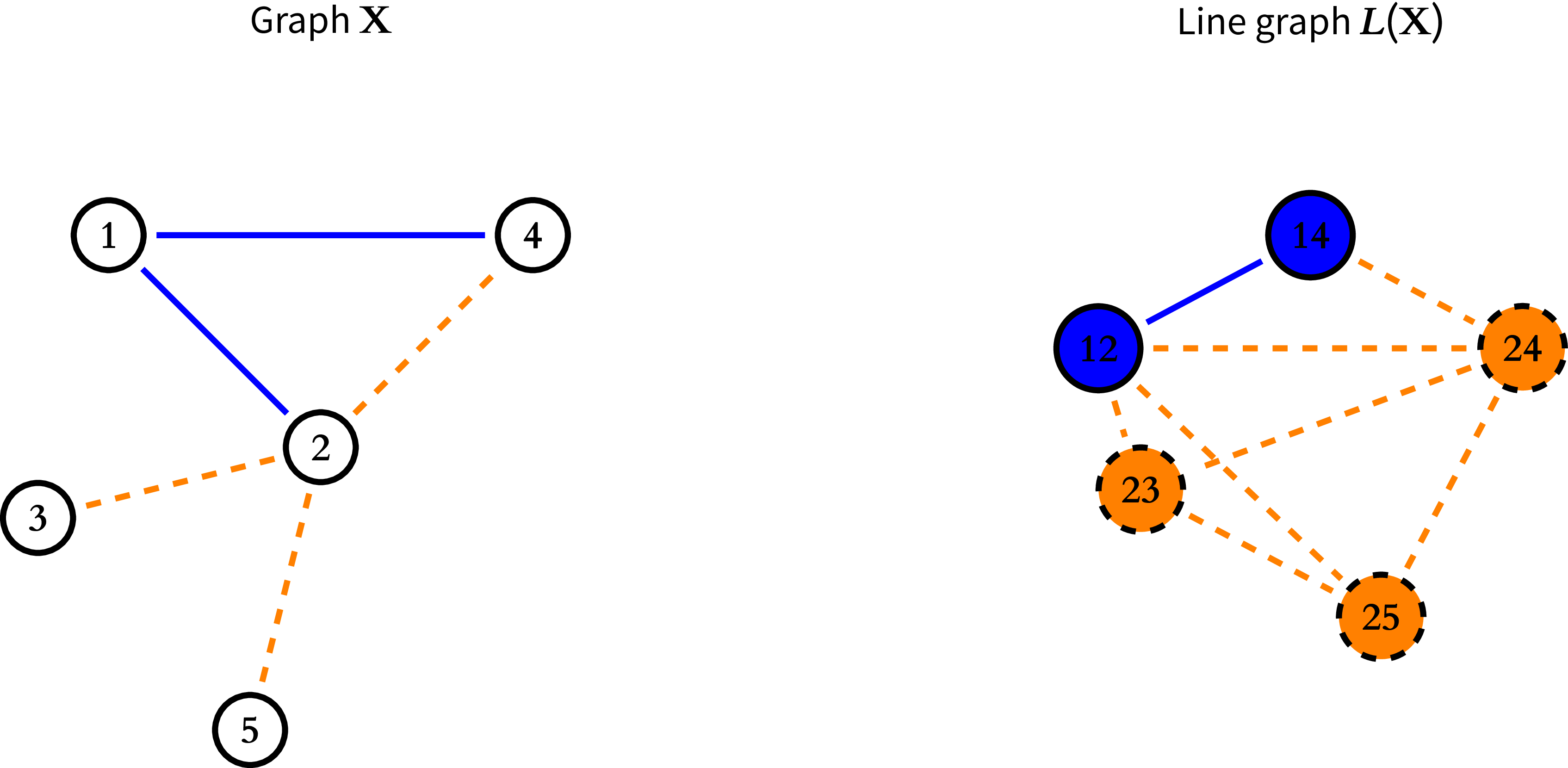
Formally following the notation introduced in Section 4, for a simple graph $G(V, E)$
with
$G(V, E)$
with $U= |E|$
edges, let
$U= |E|$
edges, let $L = L(G)$
be the line graph of
$L = L(G)$
be the line graph of $G$
. Line graphs have previously been used to describe, for example, temporal dynamics (Broccatelli et al., Reference Broccatelli, Everett and Koskinen2016; Moody, Reference Moody2008). The vertices on
$G$
. Line graphs have previously been used to describe, for example, temporal dynamics (Broccatelli et al., Reference Broccatelli, Everett and Koskinen2016; Moody, Reference Moody2008). The vertices on $L$
are the edges
$L$
are the edges $E$
from graph
$E$
from graph $G(V,E)$
and there is an edge
$G(V,E)$
and there is an edge $\{u, v\} \in L$
if
$\{u, v\} \in L$
if $u \cap v \neq \varnothing$
. For example, if
$u \cap v \neq \varnothing$
. For example, if $u = \{i, j \}$
and
$u = \{i, j \}$
and $v = \{i, k\}$
and
$v = \{i, k\}$
and $\{i, j\}, \{i, k\} \in E$
, then
$\{i, j\}, \{i, k\} \in E$
, then $\{u, v\} \in L$
.
$\{u, v\} \in L$
.
In plain language, the vertices in the line graph $L$
correspond to the edges in the graph
$L$
correspond to the edges in the graph $G$
. Accordingly, the edges in the line graph
$G$
. Accordingly, the edges in the line graph $L$
are defined when the edges in the graph
$L$
are defined when the edges in the graph $G$
share a common node. Therefore, the line graph is a convenient format to understand why edges in a graph are related to other edges. The vertices in the line graph
$G$
share a common node. Therefore, the line graph is a convenient format to understand why edges in a graph are related to other edges. The vertices in the line graph $L(G)$
are only defined for the edges in
$L(G)$
are only defined for the edges in $E$
, and thus do not evaluate any null ties in graph
$E$
, and thus do not evaluate any null ties in graph $G$
. A relevant property expanded below is that the higher degree a node in
$G$
. A relevant property expanded below is that the higher degree a node in $G$
has, the more likely the corresponding edges’ nodes in
$G$
has, the more likely the corresponding edges’ nodes in $L$
are to have more edges, and thus higher degree. This happens because nodes in
$L$
are to have more edges, and thus higher degree. This happens because nodes in $G$
with more edges to other nodes are more likely to have adjacent edges. By emphasizing the definition of edges and omitting null ties, we believe the line graph to be a data format that conveniently represents the bias towards edge sampling.
$G$
with more edges to other nodes are more likely to have adjacent edges. By emphasizing the definition of edges and omitting null ties, we believe the line graph to be a data format that conveniently represents the bias towards edge sampling.
When we pair the line graph with the sampling indicator matrix $\mathbf{S}$
, we arrive at a useful format to represent dependence in edge sampling. As the line graph
$\mathbf{S}$
, we arrive at a useful format to represent dependence in edge sampling. As the line graph $L$
represents edges in
$L$
represents edges in $G$
as nodes, the sampling indicator matrix
$G$
as nodes, the sampling indicator matrix $\mathbf{S}$
is instead a binary vector
$\mathbf{S}$
is instead a binary vector $\mathbf{y}$
, with elements
$\mathbf{y}$
, with elements $y_u$
defined as
$y_u$
defined as
 \begin{align} y_u = \begin{cases} 0 & \text{if edge } u \text{ has not been sampled} \\ 1 & \text{if edge } u \text{ has been sampled} \end{cases}, \end{align}
for $u = 1, \ldots , U$
for the
$u = 1, \ldots , U$
for the $U$
edges in edge set
$U$
edges in edge set $E$
. As the binary sampling vector represents which edges of the graph
$E$
. As the binary sampling vector represents which edges of the graph $G$
were sampled, we can use this vector as an outcome variable of a statistical model to specify an edge sampling process.Footnote
2
We now discuss some relevant models for the line graph and binary sampling indicator vector.
$G$
were sampled, we can use this vector as an outcome variable of a statistical model to specify an edge sampling process.Footnote
2
We now discuss some relevant models for the line graph and binary sampling indicator vector.
6.1 Conditioned on the line graph
We seek to obtain a statistical model to understand why certain edges are sampled over other edges. Therefore, we model a binary sampling vector $\mathbf{y}$
while conditioning on the line graph.
$\mathbf{y}$
while conditioning on the line graph.
We first introduce a generalized linear model, specifically with a logistic link function as the model for the line graph using the binary sampling vector as the outcome variable,
 \begin{align} P(y_u = 1 | L, \theta ) = \frac {\exp \{\theta _0 + \theta _1 f_u(L)\}}{1 + \exp \{\theta _0 + \theta _1 f_u(L)\}}. \end{align}
The function $f_u(L)$
here expresses some function of the edges of the line graph for the particular
$f_u(L)$
here expresses some function of the edges of the line graph for the particular $u$
. This can be the degree of
$u$
. This can be the degree of $u$
in
$u$
in $L$
if we wanted to assume degree-based sampling biases (e.g., nodes in the line graph with more edges are more likely to be sampled). If edge covariates for the true graph
$L$
if we wanted to assume degree-based sampling biases (e.g., nodes in the line graph with more edges are more likely to be sampled). If edge covariates for the true graph $C$
were available, we can introduce heterogeneity in the model using the edge covariates,
$C$
were available, we can introduce heterogeneity in the model using the edge covariates,
 \begin{align} P(y_u = 1 | L, c_u, \theta ) = \frac {\exp \{\theta _0 + \theta _1 f_u(L)+ \theta _2 c_u\}}{1 + \exp \{\theta _0 + \theta _1 f_u(L) + \theta _2 c_u\}}. \end{align}
While this model is straightforward to implement and represents a model to describe the process that affects the probability for an edge to be sampled, this does not address the dependence between the sampled edges. Generalized linear models tend to assume independent observations and the current model is no exception. This model can be relevant if the researcher were certain that their collected set of (independent) nodal covariates are sufficient in explaining heterogeneities in the probabilities of sampling edges. In the following section, we address both of the empirical sampling biases.
6.2 Auto-logistic actor attribute model
We turn to the ALAAM (Daraganova, Reference Daraganova2008; Daraganova and Robins, Reference Daraganova and Robins2013; Koskinen and Daraganova, Reference Koskinen and Daraganova2022) to represent edge sampling processes in the line graph. While the ALAAM is primarily used to investigate social influence in cross-sectional data, it is fundamentally a model that can account for dependence among binary outcome variables by conditioning on a cross-sectional network. When conditioning on the line graph, the resulting model would substantively be able to describe the probability of sampling an edge, while accounting for all the sampled and unsampled adjacent edges in the line graph. By conditioning on the line graph, the ALAAM captures the empirical tendency to emphasize the sampling of edges instead of both edges and null ties. The model can be described in terms of its probability mass function (pmf) as
 \begin{align} P(\mathbf{y} |L, \theta ) = {\exp}{\left\{\theta ^{\top } z(\mathbf{y}, L) - \kappa (\theta )\right\}}, \end{align}
where $z()$
is a
$z()$
is a $p \times 1$
vector describing both network and attribute covariates in the model,
$p \times 1$
vector describing both network and attribute covariates in the model, $\theta \in \mathbb{R}^p$
are the natural parameters, and
$\theta \in \mathbb{R}^p$
are the natural parameters, and
 \begin{align} \kappa (\theta ) = \log \sum _{\mathbf{y} \in \mathcal{Y}} {\exp}{\left\{\theta ^{\top } z(\mathbf{y}, L) \right\}}, \end{align}
is the normalizing constant. The part of the model responsible for modeling social influence is in the model specification $z()$
. Specifically what would usually be termed a contagion parameter for general ALAAM usage can be included to reflect a “social influence” process for the sampling vector
$z()$
. Specifically what would usually be termed a contagion parameter for general ALAAM usage can be included to reflect a “social influence” process for the sampling vector $\mathbf{y}$
.
$\mathbf{y}$
.
To specify our usage of the contagion parameter in the line graph, we frame the parameter as a POI bias to reflect the bias that sampled edges are adjacent to other sampled edges. It is specified as
 \begin{align} z(\mathbf{y}, L) = \sum _{u \lt v} y_u y_v L_{uv}, \end{align}
or, more specifically, the total number of edges in the line graph where both incident vertices are indicated to be sampled ( $y_uy_v = 1$
). When we translate this to the true graph
$y_uy_v = 1$
). When we translate this to the true graph $G$
, this statistic reflects the total number of edges that are adjacent to each other, or connected through a vertex in
$G$
, this statistic reflects the total number of edges that are adjacent to each other, or connected through a vertex in $G$
.
$G$
.
In the conditional form, if the corresponding parameter is positive, then the probability that $\{ i, j\}$
is sampled is greater if another edge,
$\{ i, j\}$
is sampled is greater if another edge, $\{i,k\}$
, of
$\{i,k\}$
, of $i$
has been sampled, than if
$i$
has been sampled, than if $\{i,k\}$
has not been sampled. Therefore, sampling the ties of one “person of interest” (POI) increases the probability of sampling further ties of this person, because the ties are dependent through nodes. In other words, the POI bias (23) lets us move away from independent (random) sampling mechanisms and address biased (dependent) sampling mechanisms.
$\{i,k\}$
has not been sampled. Therefore, sampling the ties of one “person of interest” (POI) increases the probability of sampling further ties of this person, because the ties are dependent through nodes. In other words, the POI bias (23) lets us move away from independent (random) sampling mechanisms and address biased (dependent) sampling mechanisms.
This can be considered to reflect the number of 2-stars in the network, which in turn resembles the simplest Markov dependence assumption as described in Frank and Strauss (Reference Frank and Strauss1986). When we use the ALAAM as the model, we can use the POI bias parameter to tune the levels of dependence between the edges being sampled. Specifying different levels of dependence allows a systematic model-based approach that can substantively allow us to describe edge sampling designs with different levels of dependence between sampled edges.
In addition to being a methodologically convenient parameter, the POI bias parameter encapsulates the empirical biases of sequential sampling. The literal interpretation of the parameter is one that modulates the extent to which edges (in the network) are more (or less) likely to be sampled if they were adjacent to other edges. This captures the sequential (e.g., “spotlight”) effects in covert network sampling. In addition to capturing sequential sampling artifacts through the POI bias, the use and conditioning of the line graph reflects the empirical preference of edges over null ties. Therefore, the ALAAM is the model of choice for our aim to generate realistic empirical sampling biases.
6.3 The distribution of networks implied by edge sampling
As explored in Section 5, analytical results for edge sampling mechanisms are only available for independently sampled edges and simple summary statistics. The question then follows of what can be said for the novel approach to represent dependence between sampled edges through an ALAAM on the sampled graph’s line graph. We will briefly illustrate why analytical results are unavailable and that we have to rely on Monte Carlo methods to inspect the distribution on graphs that results from dependent edge sampling.
We define an edge sampling process for $\mathbf{S}$
. For independent sampling the pmf is a straightforward product of sampled edges and non-sampled edges
$\mathbf{S}$
. For independent sampling the pmf is a straightforward product of sampled edges and non-sampled edges
 \begin{align} P(\mathbf{S} \mid \mathbf{X})=\prod _{i\lt j}\left [x_{ij}p^{s_{ij}}(1-p)^{(1-s_{ij})}+(1-x_{ij})(1-s_{ij})\right ], \end{align}
and Frank (Reference Frank1971) derives some properties of the distributions $P(f(\mathbf{S, \mathbf{X}}) \mid \mathbf{X})$
, for some functions
$P(f(\mathbf{S, \mathbf{X}}) \mid \mathbf{X})$
, for some functions $f\,:\,\mathcal{S}\times \mathcal{X}\rightarrow \mathbb{R}$
. However, we find independent sampling to be unrealistic for the purposes of representing the discovery process of covert networks by law enforcement or police organizations.
$f\,:\,\mathcal{S}\times \mathcal{X}\rightarrow \mathbb{R}$
. However, we find independent sampling to be unrealistic for the purposes of representing the discovery process of covert networks by law enforcement or police organizations.
Expression (21) is the pmf of $\mathbf{y}$
which is a vector of indicators of whether the
$\mathbf{y}$
which is a vector of indicators of whether the $s_{ij}=1$
or
$s_{ij}=1$
or $s_{ij}=0$
, where
$s_{ij}=0$
, where $L=L(\mathbf{X})$
is the line graph on
$L=L(\mathbf{X})$
is the line graph on $\mathbf{X}$
that maps the ties of
$\mathbf{X}$
that maps the ties of $\mathbf{X}$
to the elements of
$\mathbf{X}$
to the elements of $\mathbf{y}$
. The distribution
$\mathbf{y}$
. The distribution $P(\mathbf{y} \mid L, \boldsymbol{\theta })$
is not analytically tractable because of the normalizing constant
$P(\mathbf{y} \mid L, \boldsymbol{\theta })$
is not analytically tractable because of the normalizing constant $\kappa (\boldsymbol{\theta })$
, meaning that the probability for any
$\kappa (\boldsymbol{\theta })$
, meaning that the probability for any $\mathbf{y} \in \mathcal{Y}$
is unknown. For any realization of
$\mathbf{y} \in \mathcal{Y}$
is unknown. For any realization of $\mathbf{y}$
we may construct a sampled graph
$\mathbf{y}$
we may construct a sampled graph $\mathbf{X}^{\ast }$
, as
$\mathbf{X}^{\ast }$
, as $\mathbf{X}^{\ast }=g(\mathbf{y},L)$
. As the distribution for
$\mathbf{X}^{\ast }=g(\mathbf{y},L)$
. As the distribution for $\mathbf{y}$
is intractable, so is the induced distribution
$\mathbf{y}$
is intractable, so is the induced distribution
 \begin{align} P(\mathbf{X}^{\ast } \mid L, \boldsymbol{\theta })= \sum _{\mathbf{y}:g(\mathbf{y},L)=\mathbf{X}^{\ast }}P(\mathbf{y} \mid L, \boldsymbol{\theta }). \end{align}
Note that just because $x^{\ast }_{ij}=0$
, we do not know whether
$x^{\ast }_{ij}=0$
, we do not know whether $\{i,j\}$
is a node of
$\{i,j\}$
is a node of $L(\boldsymbol{X})$
.
$L(\boldsymbol{X})$
.
While we can understand the conditional distribution of $y_u \mid \mathbf{y}_{-u}$
in terms of a Bernoulli trial with a closed-form pmf, the distribution for
$y_u \mid \mathbf{y}_{-u}$
in terms of a Bernoulli trial with a closed-form pmf, the distribution for $\mathbf{y}$
defined in (21) is intractable and so is the distribution
$\mathbf{y}$
defined in (21) is intractable and so is the distribution $P(\mathbf{X}^{\ast } \mid L, \boldsymbol{\theta })$
. Consequently we can only explore
$P(\mathbf{X}^{\ast } \mid L, \boldsymbol{\theta })$
. Consequently we can only explore $P(\mathbf{X}^{\ast } \mid L, \boldsymbol{\theta })$
using Monte Carlo methods. Similarly, for functions
$P(\mathbf{X}^{\ast } \mid L, \boldsymbol{\theta })$
using Monte Carlo methods. Similarly, for functions $f\,:\,\mathbf{X}^{\ast }\rightarrow \mathbb{R}$
, such as counts of certain structures in the sampled graph, the distribution
$f\,:\,\mathbf{X}^{\ast }\rightarrow \mathbb{R}$
, such as counts of certain structures in the sampled graph, the distribution
 \begin{align} P(z)=\sum _{\mathbf{X}^{\ast }\,:\,f(\mathbf{X}^{\ast })=z}P(\mathbf{X}^{\ast } \mid L, \boldsymbol{\theta }) \end{align}
cannot be evaluated analytically. These distributions are presented in following simulations’ figures for different choices of $\mathbf{X}$
and
$\mathbf{X}$
and $\boldsymbol{\theta }$
.
$\boldsymbol{\theta }$
.
7. Simulations and implications
The following simulations use the ALAAM as a model for the line graph (21). We used three different models in our simulations to reflect three different edge sampling mechanisms. The model specification was identical, but the three models had three levels of dependence.
The POI bias parameter, parameterized as above (23), was included with varying levels. The three levels of dependence were (a) zero, to reflect an independent model similar to logistic regression, (b) small, to reflect minor dependence between sampled edges, and (c) large, to reflect a substantial dependence between sampled edges. The different levels of dependence were specified as different target mean value parameters in the simulation of the ALAAM. We transformed a dyadic covariate (age difference) for the adjacency matrix to a monadic variable of the line graph as a proof of concept for adapting dyadic covariates for the line graph.
7.1 Empirical covert network
To conduct simulations of the sampling processes, we first obtained the line graph of a target “true” network and specified a proportion of sampled edges. For the first set of simulations, we used an empirical covert network from the UCINet covert network repository. Specifically the London Gangs network as attributes of the actors were available as well (Grund and Densley, Reference Grund and Densley2015). The network (Figure 3) has 54 nodes and a density of 0.093. We sampled 65% of the network.
The London gangs dataset.
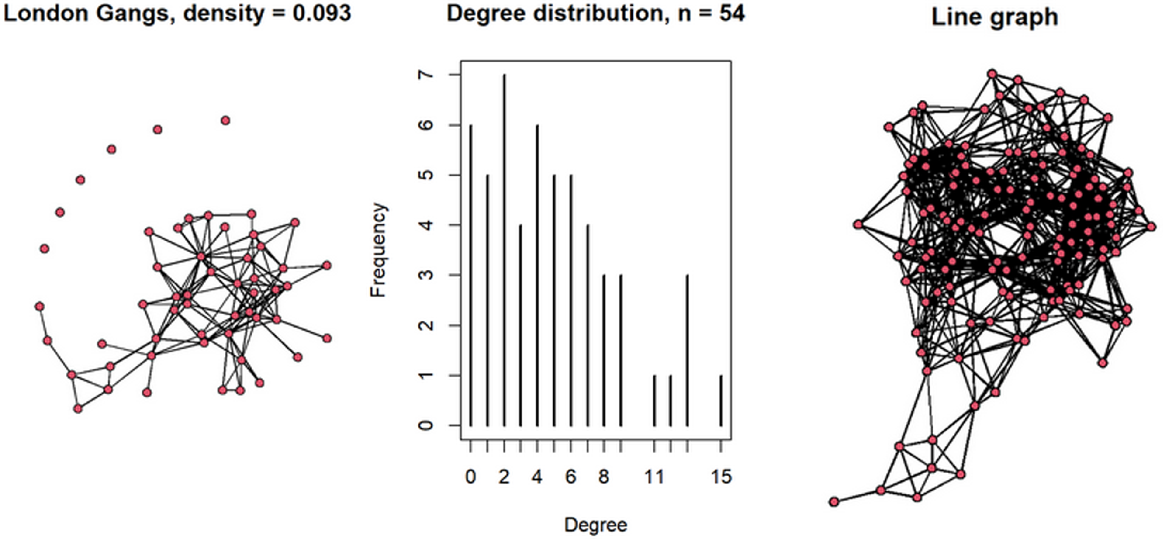
Figure 3 Long description
Panel A: A network graph shows the connections between members of London gangs. The nodes represent gang members, and the edges represent their connections. The graph is sparse with a density of 0.093, indicating that not all possible connections are present. Panel B: A histogram displays the degree distribution of the network, with the x-axis labeled Degree and the y-axis labeled Frequency. The degrees range from 0 to 15, and the frequencies vary, showing how many nodes have each degree. Panel C: Another network graph, labeled Line graph, provides a different visualization of the same network, highlighting the interconnectedness of the gang members.
The three different sampling processes were formulated as different levels of target counts in $\mathbf{S}$
, with zero being
$\mathbf{S}$
, with zero being $0$
, small and large depending on the number of observed POI bias in the target network (Figure 4).
$0$
, small and large depending on the number of observed POI bias in the target network (Figure 4).
Examples of sampled empirical covert networks with different POI bias levels.

We implemented a density-conditioning step to ensure the sampled network had approximately the same density across different sampling processes (Appendix A). This step is important in the following simulations to ensure that differences in the following descriptive statistics are due to the different biased sampling procedures, and not because of a difference in the number of sampled edges.
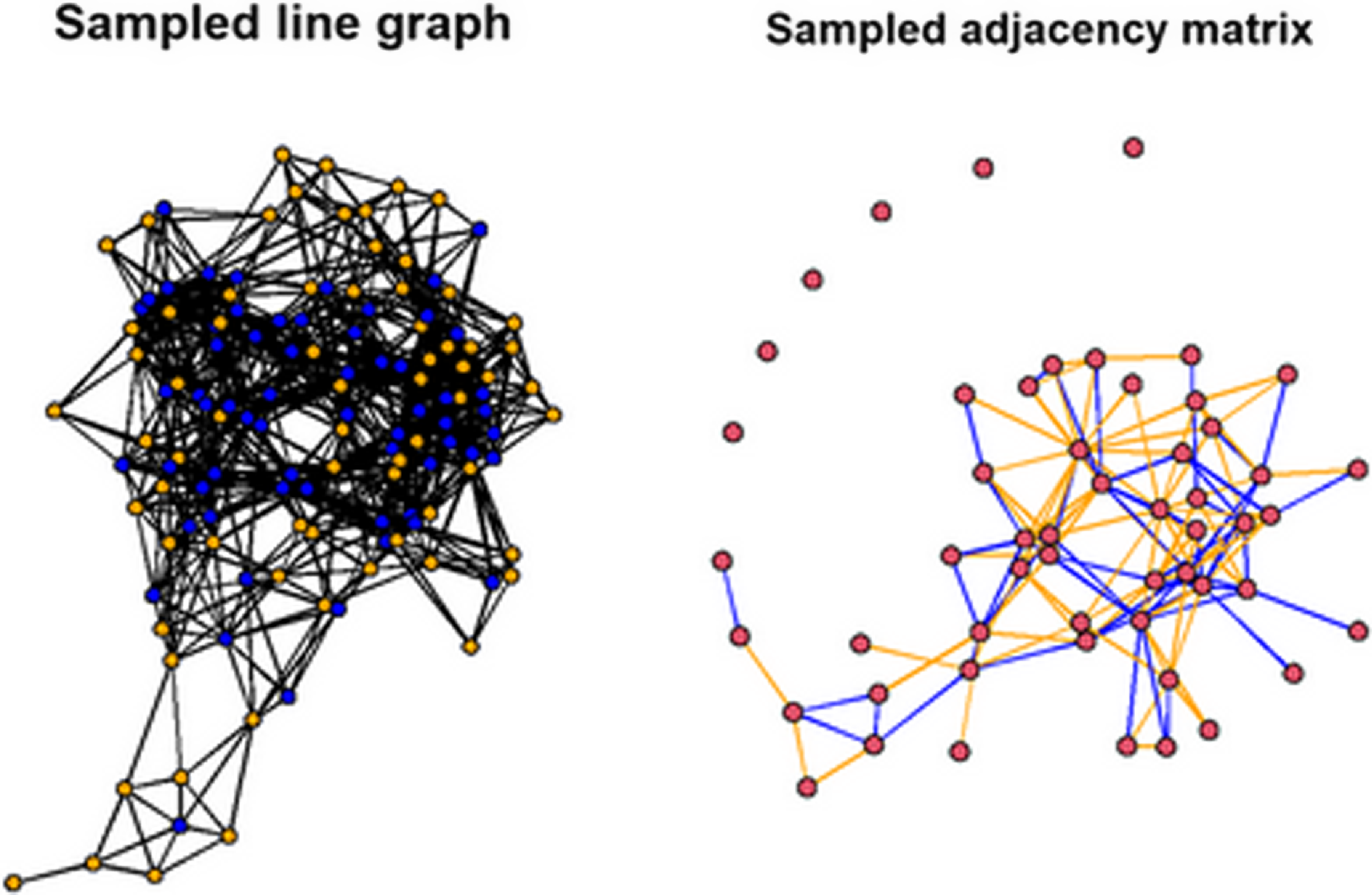
After ensuring the sampled line graphs could be compared, they were transformed back to sampled adjacency matrices (Figure 5). The blue nodes in the line graph correspond to the sampled edges in the sampled adjacency matrix while the orange nodes in the line graph are unsampled edges in the adjacency matrix. We then inspected various network metrics of the sampled adjacency matrices, including betweenness centrality, global centralization, clustering coefficient, and path length measures including average geodesic and diameter using density plots of the 10000 draws of each model.
Sampled line graph and corresponding adjacency matrix.
As seen in Figure 6a, the density-conditioning step is successful as the densities of the sampled adjacency matrices are very similar across the three sampling models. The levels of dependence were also notably different between the three models (Figure 6b), which is evidence to suggest that the three different sampling model specifications were able to simulate different levels of dependence between sampled edges. The blue vertical line in the density plots refers to the value of the metrics in the true network, however it is purely for reference purposes and is not a target for the simulations as we are not sampling the entire network.
Empirical covert network diagnostics.

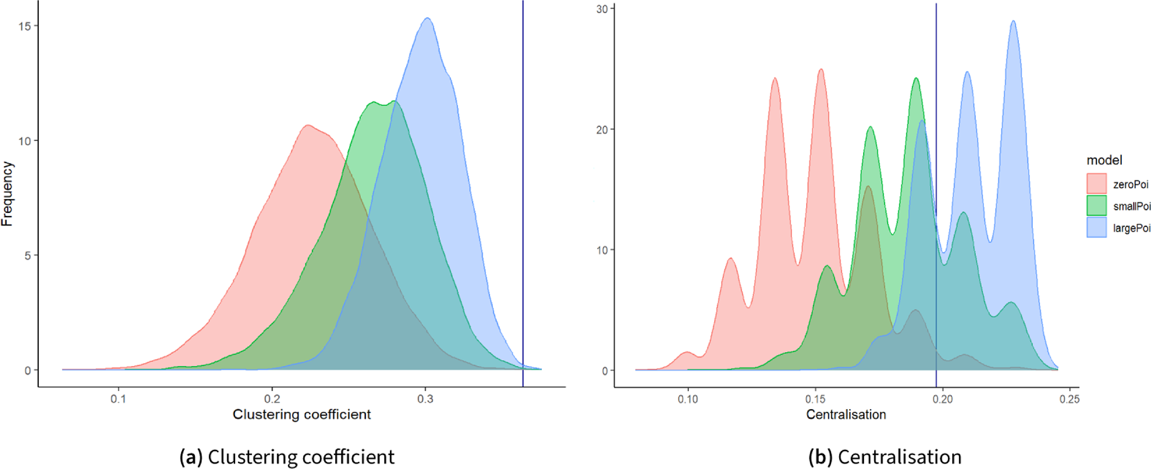
The next set of density plots inspected global metrics for the clustering and degree centralization of the sampled adjacency matrices. As seen from Figure 7a, the three sampling regimes resulted in adjacency matrices with different clustering coefficients. Particularly, the large dependence model has a larger clustering coefficient compared to the other two models. This finding means that the simulated sampled adjacency matrices where we assumed a high level of dependence between sampled edges had a higher tendency to cluster together.
Empirical covert network global metrics.
Empirical covert network path length metrics.

Figure 8 Long description
Panel A: A density plot shows the distribution of diameter values for three models: zeroPoI, smallPoI, and largePoI. The x-axis represents the diameter, and the y-axis represents the frequency. The zeroPoI model is represented in red, the smallPoI model in green, and the largePoI model in blue. Each model shows distinct peaks at different diameter values. Panel B: Another density plot displays the distribution of average geodesic values for the same three models. The x-axis represents the average geodesic distance, and the y-axis represents the frequency. The zeroPoI model is shown in red, the smallPoI model in green, and the largePoI model in blue. Each model exhibits different distribution patterns across the average geodesic values.
Substantively speaking, this means that relying on sampled edges to inform further sampling of related edges may result in a sampled network that has a clustered structure as a result of the sampling mechanism alone. The same phenomena can be seen in the global centralization comparative density plot (Figure 7b). We see that the high dependence model has a higher centralization value compared to the other two models. As global centralization reflects the variance of the degree distribution (Freeman et al., Reference Freeman, Roeder and Mulholland1979), the sampled adjacency matrices of the large dependence model have larger variance in the degree distribution which corresponds to a more centralized network. The peaks within the distributions in centralization likely reflects differing numbers of sampled connected subgroups, with fewer connected subgroups increasing the centralization value. This finding illustrates how the POI bias can be tuned to reflect sampled mechanisms with varying levels of dependence.
The geodesic distance and diameter plots (Figure 8) both show that the path lengths of the sampled adjacency matrices of the high dependence model are smaller than the other two models. While smaller path lengths generally reflect higher connectivity, due to the density-conditioning manipulation, the smaller path lengths could be understood as an artifact of sampling a highly connected component, while failing to sample less connected nodes. We also see a larger quantity of isolates in the sampled networks with large dependence (Figure 9b).
Empirical covert network connectivity metrics.

It is evident that the more likely adjacent edges are to be sampled, edges involving peripheral members are more likely to be missed, especially with finite sampling resources. The rising isolate count as sampling dependence increases supports this claim. Intuitively, we can see that primarily sampling the connected members and their edges makes it difficult to sample members who are not within the same subgraph. This results in fewer sampled edges involving peripheral members belonging to different subgraph structures.
The presented simulations may inform sampling decisions. If the primary goal is identifying the most amount of individuals, we see that independent sampling is preferred as this sampling mechanism generated the least isolates. If we wanted to sample subgraph structures instead, we see that highly dependent sampling is more likely to identify individuals in connected components. The ALAAM is ultimately successful as a generative model to simulate different sampling mechanisms for an empirical covert network. However, the generalizability of these findings is a very pertinent question. This brings us to the following set of simulations.
7.2 Varying random graphs
The following simulations extends the same simulation methodology on some different true networks. We were primarily interested in investigating whether structure in a sampled network could be understood as an artifact of the sampling mechanism. In other words, we are interested in whether something that is not a social network may result in a seemingly highly structured social network, as a function of a biased edge sampling process.
7.2.1 Triangle-dense random graph
In this investigation, we simulated random graphs with some added triangles as the population network. In the following simulations, we included triangles in the generation of the random graphs because completely random graphs did not have sufficient structure to infer whether different sampling mechanisms can overemphasize the occurrence of social structures from the random networks. For illustrative purposes, we opted to use a similar method as the dyad census conditioned random graphs, or UMAN distributions. As the UMAN distributions are generalizations of the Erdos-Renyi case, we aimed to obtain a distribution of graphs conditional on the number of triangles. Further details of the simulation are described in Appendix B.
After sampling graphs from the target distribution, we performed the sampling simulations as described above on the sampled graph (Figure 10). We sampled 50% of the population network to make the simulation run smoother because smaller samples of population network led to simulation difficulties, likely due to fewer observation of certain statistics. Similar to the previous set of simulations, the vertical line depicts the true statistic for the full network. However, the goal of the following simulations is not to see which sampling mechanism is closest to the true value. We are more interested in differences between the sampled network with different sampling mechanisms. We can see how the different sampling mechanisms sampled the triangle-dense random graphs in Figure 11.
A simulated random graph with a high level of clustering.

Sampled triangle-dense random graphs with different POI bias levels.

As seen from the density plots below, the density-conditioning step was also successful (Figure 12(a)), however the variance of the sampled networks of the large dependence model seem to be larger than the other two models. The same pattern in the variance can be seen in the POI bias (Figure 12(b)). As this pattern was not found in the simulation using the empirical covert network, the explanation for why the variance is increasing here lies in the target network being a random graph. We suspect this is explained by the density-conditioning step we implemented. Some further details can be found in Appendix A.
Triangle-dense random graphs diagnostics.

According to the results, the clustering coefficient and centralization density plots (Figure 13) seem fairly similar to the empirical covert network. Both the clustering coefficient and centralization values are higher in the large dependence model, thus suggesting that having more dependence between sampled edges can lead to sampled networks with that appear to be noticeably more connected and cohesive when compared to the independent sampling of edges.
Triangle-dense random graphs global metrics.

The average geodesics, diameter, and average betweenness centrality of the sampled networks (Figures 14 & 15(a)) from the large dependence model describe a similar story to the previous set of simulations. The smaller average geodesics and diameter suggest that the sampled networks have a smaller path length and are generally more connected than sampling mechanisms that have smaller levels of dependence. The smaller average betweenness further supports the effect of the sampling mechanism as we can understand the decreasing betweenness centrality as a function of the increasing connectedness in the sampled network. The increasing number of isolates (Figure 15(b)) can also be seen as an effect of predominantly sampling edges adjacent to other edges, resulting in sampling fewer peripheral members.
Triangle-dense random graph path length metrics.

Figure 14 Long description
Two density plots compare the distribution of diameter and average geodesic for different models. Panel A: The density plot shows the distribution of diameter for three models: zeroPo (red), smallPo (green), and largePo (blue). The x-axis represents the diameter with units, and the y-axis represents the frequency. The plot shows multiple peaks and variations in the distribution for each model. Panel B: The density plot shows the distribution of average geodesic for the same three models. The x-axis represents the average geodesic with units, and the y-axis represents the frequency. The plot shows overlapping distributions with different peaks and spread for each model.
Triangle-dense random graph connectivity metrics.

The findings above demonstrate trade-offs for different sampling mechanisms. With different levels of the POI bias and a similar sampled density, we can inspect the result of sampling mechanisms with different levels of dependence between sampled edges. We see that for sampling mechanisms with a large POI bias, there is a tendency for the sampled network to be more connected and cohesive (i.e., larger clustering coefficient and centralization, smaller path length metrics) compared to the independent sampling mechanism. However, we also see that that the large POI bias sampling mechanism also has the most isolates. In other words, additional structure is sampled at the cost of fewer sampled actors.
These findings are to be expected when the contagion parameter of the ALAAM of the line graph is set to be positive (POI bias; (23)), however the exact outcomes and the overall differences between sampling mechanisms are difficult to enumerate analytically (Section 6.3). For a given number of sampled edges, a tendency to focus on existing sampled edges to sample adjacent edges may intuitively lead to finding more triangles or a generally more cohesive network. However, the current simulation framework lets us inspect by exactly how much different sampling mechanisms affect the sampled network.
7.2.2 Simulated co-arrest
Our last set of simulations aim to reflect the sampling of discrete groups that may not necessarily represent a social network. The observation of groups or events have been recent developments in the analysis of covert networks. Some examples include groups of individuals that have been arrested or related to an illicit event together (Bright et al., Reference Bright, Sadewo, Lerner, Cubitt, Dowling and Morgan2024; Carrington, Reference Carrington2009; Hashimi et al., Reference Hashimi, Bouchard, Morselli and Ouellet2016).
In this set of simulations, we consider a population network that reflects very loosely connected group structures. According to Carrington (Reference Carrington2011), research on co-offending networks find that they tend to consist of many smaller and denser subgroups that are loosely linked together with sparse connections. The sparsely-connected subgroups appear to be a network, but the consequences of constructing networks from data that are not specifically collected to construct a network has scarcely been investigated.
We adopt the conceptual framework of a blockmodel (White et al., Reference White, Boorman and Breiger1976) to simulate our population network. We specify a number of blocks that are fully connected within the block to reflect group memberships between individuals and limit the amount of connections between blocks to reflect sparse connections between the smaller subgroups. The simulated population network and its one-mode projection can be seen in Figure 16. That is, the two modes in the bipartite network are collapsed into one mode indicating co-membership of a common block. We also sampled 50% of the population network in this set of simulations. The different sampled networks can also be seen in Figure 17.
A random bipartite network and its one mode projection.

Sampled projected networks with varying sampling POI bias.

Upon inspection of the density and POI bias levels (Figure 18), we can see that this set of simulations is more volatile than the previous ones. While the density is comparable on average, we can see that the spread of the high dependence distribution seems to be multimodal. A similar multimodal distribution can be seen in the distribution of the POI bias parameter.
Random projected network diagnostics.

Figure 18 Long description
Two density plots compare different models based on density and POI bias. Panel A: The density plot shows the frequency distribution of density values for three models: zeroPoI, smallPoI, and largePoI. The x-axis represents density, and the y-axis represents frequency. The zeroPoI model is represented in red, the smallPoI model in green, and the largePoI model in blue. Panel B: The density plot shows the frequency distribution of POI bias values for the same three models. The x-axis represents POI bias, and the y-axis represents density. The zeroPoI model is represented in red, the smallPoI model in green, and the largePoI model in blue.
The explanation for the multimodal distribution lies in the structure of the one-mode projected network. As illustrated in Figure 16, the projected network has multiple connected subgraphs. Sampling edges within each of these subgraphs would be very likely as the individual components are fully connected. In contrast, sampling edges between these components are very unlikely. This led to the multimodal distributions of density and POI bias as some simulations sampled more connected components than others.
The clustering coefficient and centralization density plots for the simulated co-arrest networks (Figure 19) are very similar to the previous simulations. However, the clustering coefficients are more prominently affected by the levels of dependence here when compared to the other two simulations. This is similarly explained by the modular structure of the one-mode projection as there are many closed triangles but only a few open triangles in the connected subgraphs.
Random projected network global metrics.

The path length density plots (Figures 20 & 21(a)) also demonstrated similar tendencies to the previous simulations. We see that the high dependence sampled networks have smaller path lengths on average. In contrast to the previous simulations, we also see that the level of dependence had a more prominent effect in distinguishing the path length measures. This is also understood to be the product of sampling clustered subgroups as high sampling dependence makes it more likely for within-group edges to be sampled than the few between-group edges in the simulated network. As a result, the path lengths of the high dependence sampled networks are smaller than the independently sampled networks.
The disparity in the isolates are especially striking in this set of simulations as well (Figure 21(b)). The high sampling dependence sampled networks had a large amount of isolates. We can attribute this to the highly compartmentalized subgraph structures in the projected networks. As edges belonging to nodes within each group are more likely to be sampled, edges that exist between nodes from different groups are unlikely to be sampled. The isolate count is a consequence of such a bias. As the relational information within the groups are likely to be sampled, the sample can seem to be filled with isolates due to concentrating on the nodes from known group memberships.
Random projected network path length metrics.

Figure 20 Long description
Two density plots compare the distribution of diameter and average geodesic distance across different models. Panel A: The density plot shows the distribution of diameter for three models: zeroPoI, smallPoI, and largePoI. The x-axis represents the diameter, and the y-axis represents the frequency. The zeroPoI model shows a peak around a diameter of 2, the smallPoI model peaks around a diameter of 4, and the largePoI model shows a broader distribution with peaks around diameters of 2 and 6. Panel B: The density plot shows the distribution of average geodesic distance for the same three models. The x-axis represents the average geodesic distance, and the y-axis represents the frequency. The zeroPoI model shows a peak around an average geodesic distance of 1, the smallPoI model peaks around 1.2, and the largePoI model shows a broader distribution with peaks around 0.8 and 1.4.
Random projected network connectivity metrics.

Intuitively with the clustered component structure of the projected networks, we see that having a high level of dependence led to the biased sampling of within-group ties. This leads to sampling more overall clustering, shorter path lengths, and more isolates. However, as seen in the multimodal density distribution, this could mean sampling overall fewer edges if a between-group edge is not sampled. In the pragmatic context of using co-arrest data, our findings suggest that having a high level of dependence when sampling edges leads you to find more members of the same group and ignoring individuals belonging to other groups. Further emphasizing how these simulations can inform resource allocation, we suggest having more independent sampling choices (i.e., pursuing a wider variety of information sources instead of already-collected sources) can be useful when finding other relevant groups or some potential between-group edges.
8. Discussion
In this paper, we set out to elaborate empirical biases in covert network sampling and demonstrated an application of the ALAAM to model edge sampling processes with dependence assumptions. The emphasis of edge sampling comes from the difficulty of confirming null ties between potential covert actors while the inclusion of dependence assumptions stems from the implausibility of independently sampled edges. In particular, we explore a statistically-principled method to model the discovery of edges that is consistent with empirical covert network biases.
We identify the line graph as a convenient format to represent dependencies between sampled edges and describe some models for the line graph to represent edge sampling processes which incorporate dependence assumptions. In particular, we propose using the ALAAM as contagion parameter represents a POI bias to tune the level of dependence between sampled edges. The dependence of sampled edges through nodes is a plausible representation of how analysts may learn about the network. In our examples of applying the ALAAM as an edge sampling process, we find that a high level of dependence in the sampling of edges can result in a highly structured sampled network regardless of the true network.
Substantively, the more POI bias there is in the edge sampling process, the more likely the sampled network is to bias towards connected and cohesive structures at the cost of sampling fewer nodes. In our investigations of edge sampling processes with varying levels of dependence across multiple networks, we consistently sampled more structured and centralized networks, with fewer sampled nodes, as the level of dependence increases. Specifically, as the level of dependence increases, the sampled networks have higher clustering coefficients and global centralization while having shorter path lengths. Practically speaking, this implies that a centralized or clustered network may be overemphasized due to a biased sampling process instead of the true network’s structure.
Our simulations also highlight a tradeoff between sampling connected subgraphs and more peripheral individuals with few edges. Under resource constraints, sampling more clustered and centralized networks comes with sampling more isolates. Through our simulations, we also find different sampling mechanisms to be preferred for different purposes. If the investigation wants to identify well-connected subgroups, focusing on already-identified individuals and their social ties will make it more likely to identify groups within the network. However, if the target of the investigation is to identify a larger number of individuals in the network, we find an independent sampling mechanism to be preferred. Practically, if the target is to find as many people related to network as possible, it is better to save resources focusing on specific individuals and subgroups. Instead, those resources can be spent to find individuals related to the network. This work is novel in the demonstration of the implicit sampling biases in the construction of covert networks and their effects on the sampled network.
There are a number of extensions that can be explored from the simulation method as described here. As the ALAAM is generally used as a statistical model to model various dependence and covariate effects on binary outcomes, a simple extension is to explore different model specifications and how they affect the resulting sampled networks. Straightforward extensions can acknowledge the multiplex or bipartite data through the choice of model specifications. While model specification in network models is typically discussed when considering the estimation of the network and its theoretically-guided social processes (Handcock, Reference Handcock2003; Lusher et al., Reference Lusher, Koskinen and Robins2013; Snijders, Reference Snijders, van Dujin and Hagberg2002), we note how the model specification of the ALAAM for the line graph can capture theoretically or empirically-relevant processes as well (Januar et al., Reference Januar, Colin Gallagher and Koskinen2026). Future extensions may also extend the application of the modeling framework for the purpose of measurement models since the model fundamentally describes the probability of a sampled edge.
As the line graph represents edges in the network as nodes in the line graph, edge or dyad covariates can be repurposed to be node covariates in the model for the line graph. For example, if we assumed that edges involving covert actors that have been active in the covert network for a longer time are more likely to be observed, we can include a node covariate in the ALAAM to account for it. Similar to Januar et al. (Reference Januar, Colin Gallagher and Koskinen2026), we expressed these sampling biases in the POI parameter of the ALAAM. The work is novel in offering a framework to study what network features might be artifacts of observational biases.
Some further extensions for the ALAAM can include predictive purposes under ideal assumptions. If we were to assume a homogeneous sampling mechanism where unsampled edges are described by the same sampling mechanism as sampled edges, the ALAAM may be used in a predictive capacity to inform which edges are likely to be sampled. For example, if there were a set of potential edges that may exist, the model would be able to generate predictions on which of the candidate edges are the most likely to be sampled given the model specification of the ALAAM.
Additionally, the presented method could be applied to verify the accuracy of the sampled networks. To fulfill this extension, it requires data with either defined waves of sampled edges or an order to the sampled edges. This can be satisfied by timestamps of the sampled edges (e.g., arrest dates) and it may be possible to quantify the accuracy of the sampled networks and explore various model specifications to capture the sampling mechanisms.
Our aim in this manuscript is to motivate edge sampling as a realistic model for the discovery of networks. We mean this to be a tool with which area experts can quantify their knowledge so that we can explore the impacts of different sampling biases. Our examples illustrated simple mechanisms and outcomes, but straightforward extensions can be included through the model specification. An interesting future avenue is the estimation of $f(L)$
to quantify sampling biases. We have defined a model for the observed network given a true, but unknown, network. The ultimate goal would be to work out how we can draw on this model for the inverse problem of inferring the true network. This seems to us a non-trivial problem but one worth pursuing in future research.
$f(L)$
to quantify sampling biases. We have defined a model for the observed network given a true, but unknown, network. The ultimate goal would be to work out how we can draw on this model for the inverse problem of inferring the true network. This seems to us a non-trivial problem but one worth pursuing in future research.
Acknowledgements
This work was first presented in the 13th Illicit Networks Workshop on 11 Dec 2023. The authors are grateful for the comments and guidance from Chiara Broccatelli, David Bright, Garry Robins, Lucia Falzon, and Pip Pattison. The authors are also grateful for comments and input from practitioners from different agencies at the Illicit Networks Workshop, Sunbelt, and in informal conversations at other forums.
Data availability statement
The study uses publicly available data as indicated and referenced in the text. All figures and code are available at request from the corresponding author (J. Januar).
Funding statement
This project was financially supported by the project “Covert Networks: How to learn as much as possible about the structure of a network from sampled subnetworks” funded by Department of Defence, through the US Army Research Office (Grant Number W911NF-21-1-0335 Proposal 79034-NS).
Competing interests
The authors declare no conflicts of interest.
Author contributions
Jonathan Januar – Conceptualization, Formal analysis, Methodology, Software, Visualization, Writing – original draft, Writing – review & editing; H Colin Gallagher – Conceptualization, Methodology, Resources, Writing – review & editing, Supervision; Johan Koskinen – Conceptualization, Methodology, Software, Writing – review & editing, Supervision, Funding acquisition.
Appendix A. Density conditioning
To allow for comparison between sampling processes, we kept the density of the sampled adjacency matrices approximately constant between simulation models. To do this, we used a single step of the Newton-Raphson stochastic approximation algorithm to obtain proposal parameters equivalent to a specified increase of specifically contagion occurrences in the model. Specifically the step is specified as
 \begin{align} \theta ^{f+1} = \theta ^{f} - Cov_{\theta ^{f}}(z(\mathbf{y}))^{-1}M, \end{align}
where $\theta$
reflects the model parameters,
$\theta$
reflects the model parameters, $z(\mathbf{y})$
reflects the outcome vector of the simulation, and
$z(\mathbf{y})$
reflects the outcome vector of the simulation, and $M$
reflects the proposed change to the mean value parameters (or observed parameter counts). We initialized the simulated graphs using a density-conditioned random graph (i.e., UMAN) and a value of 1 for
$M$
reflects the proposed change to the mean value parameters (or observed parameter counts). We initialized the simulated graphs using a density-conditioned random graph (i.e., UMAN) and a value of 1 for $\theta ^f$
because the thetas will be updated in the algorithm. To obtain the covariance of the model, we simulated graphs with the current parameters. The subsequent step updated the proposed parameters while keeping the density constant using the Newton-Raphson step above and repeated the simulations using the updated parameters. Consequently, the resulting simulations reflected sampled line graphs with increasing levels of edge dependence, all while keeping the density constant.
$\theta ^f$
because the thetas will be updated in the algorithm. To obtain the covariance of the model, we simulated graphs with the current parameters. The subsequent step updated the proposed parameters while keeping the density constant using the Newton-Raphson step above and repeated the simulations using the updated parameters. Consequently, the resulting simulations reflected sampled line graphs with increasing levels of edge dependence, all while keeping the density constant.
We also make a note of applying this step for the random graphs as in Section 7.2. As the density-conditioning step attempts to increase the POI bias parameter while holding constant the other parameters of the model, the lack of structure in the network led to difficulties in finding a set of proposal parameters. Intuitively, the random graphs had a larger disparity of isolated and highly clustered nodes. This disparity led to more variance in the density-conditioning step.
Upon inspection of the random graphs, we see that too large of a proposed change in the vector $M$
or too much covariance in the reference model can lead the simulation to fail as the simulated statistics can turn degenerate. Regardless, after some attempts of adjusting increment values and model specifications for the random true network, we were still able to simulate sampled networks that had a similar average density and different average levels of dependence.
$M$
or too much covariance in the reference model can lead the simulation to fail as the simulated statistics can turn degenerate. Regardless, after some attempts of adjusting increment values and model specifications for the random true network, we were still able to simulate sampled networks that had a similar average density and different average levels of dependence.
Appendix B. Simulating triangle-dense graphs
To generate random graphs with some level of clustering, we follow Banks and Constantine (Reference Banks and Constantine1998) and specifying a target mean triangle count. We specify the probability mass function with a specified triangle count and used an MCMC with simulated annealing to sample graphs from the target distribution. Note that we could have used a Markov triangle model to define the expected target distribution.
Notationally, we denote the target number of triangles as $\tau$
, and
$\tau$
, and $T(x)$
would correspond to the number of triangles in the graph
$T(x)$
would correspond to the number of triangles in the graph $x$
,
$x$
, $T\,:\,X \rightarrow \mathbb{R}$
. The objective function would then be
$T\,:\,X \rightarrow \mathbb{R}$
. The objective function would then be $h(x) = (T(x) - \tau )^2$
and the target distribution is specified as
$h(x) = (T(x) - \tau )^2$
and the target distribution is specified as $g_\theta (x) \propto \exp \{-\theta h(x) \}$
. Therefore, after initializing the graph
$g_\theta (x) \propto \exp \{-\theta h(x) \}$
. Therefore, after initializing the graph $x_0$
, the
$x_0$
, the $i$
-th step of a loop with
$i$
-th step of a loop with $N$
iterations would be
$N$
iterations would be
-
1. Propose a graph with some proposal function $q(X^*|X_{i-1})$
-
2. Incrementing
$\theta _{i - 1}$
to
$\theta _i$
using simulated annealing tuned by a parameter
$s$
\begin{equation*}\theta _i = s\theta _{i -1}\end{equation*}
-
3. With probability
$\min \{1, \text{H}\}, \ \text{set} \ X_i \, :\!= \, X^*$
where,otherwise
\begin{equation*}H = \frac {g_{\theta _i}(X^*)}{g_{\theta _i}(X_{i-1})},\end{equation*}
$X_i \, :\!= \, X_{i-1}$





In our simulations, we opted to swap ties with null ties (Corander et al., Reference Corander, Dahmström and Dahmström1998; Snijders and Duijn, Reference Snijders, van Dujin and Hagberg2002) as the proposal function $q()$
, set the tuning parameter
$q()$
, set the tuning parameter $s = 1.01$
and the target triangles
$s = 1.01$
and the target triangles $\tau = 60$
as to generate a random graph with a clustering coefficient of roughly 0.5. We initialized the algorithm with a random graph with a fixed order and density.
$\tau = 60$
as to generate a random graph with a clustering coefficient of roughly 0.5. We initialized the algorithm with a random graph with a fixed order and density.

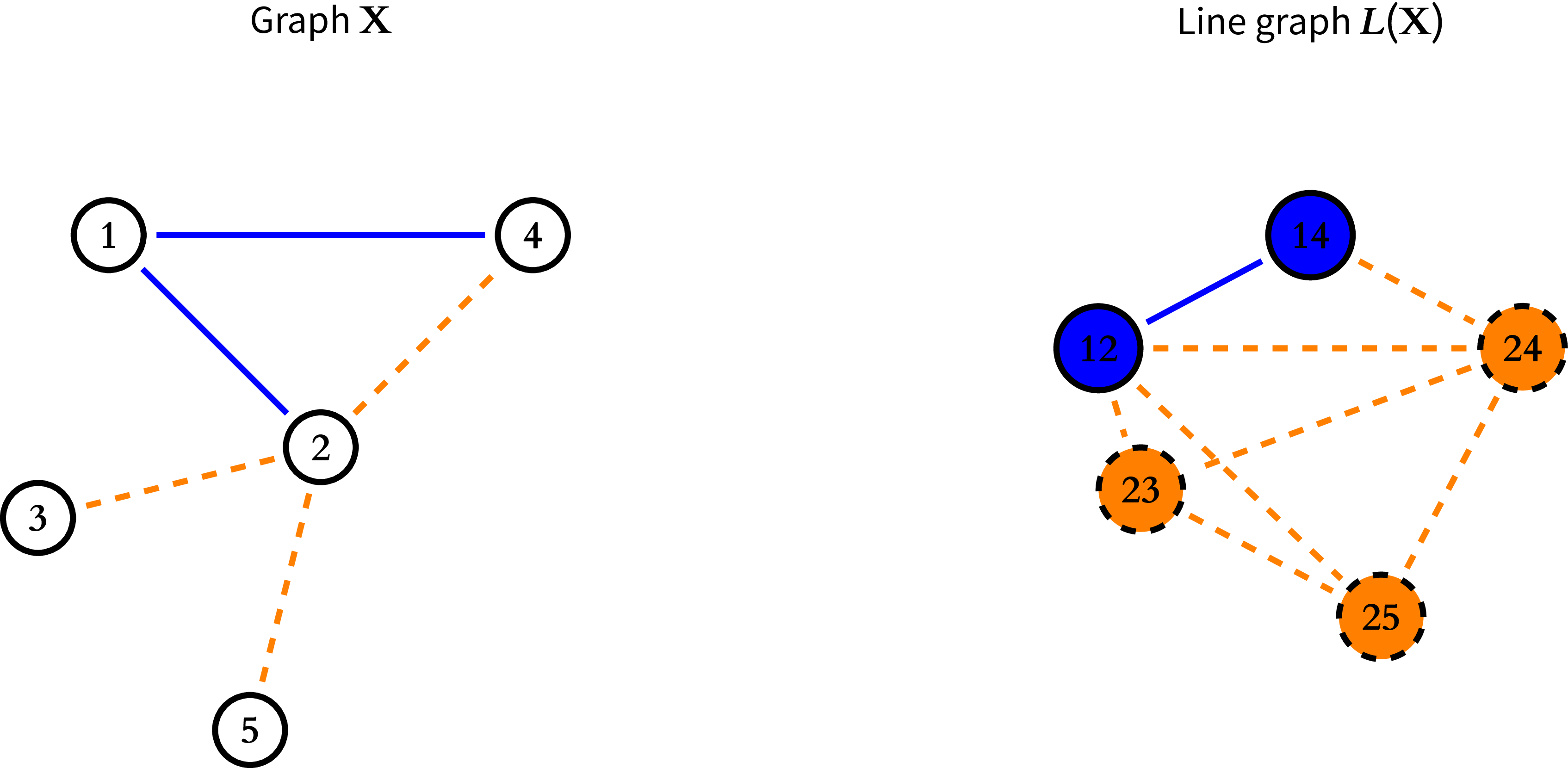
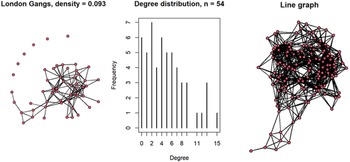
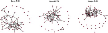
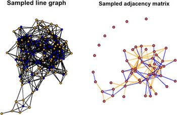
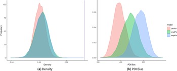
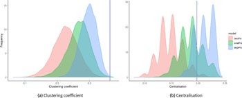
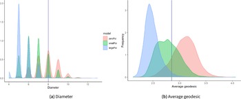

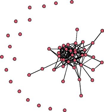


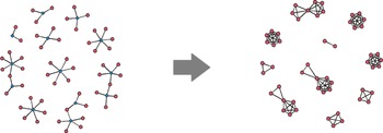
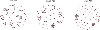


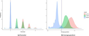
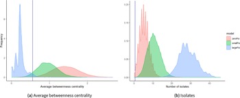

 Open access

