


1. Introduction
Given that the discrepancy between the Planck 2018 CMB measurement of $H_0$
,
$H_0$
, $67.4\pm0.5$
km s
$67.4\pm0.5$
km s $^{-1}$
Mpc
$^{-1}$
Mpc $^{-1}$
(Planck Collaboration et al. Reference Collaboration2020) and most recent SH0ES measurement,
$^{-1}$
(Planck Collaboration et al. Reference Collaboration2020) and most recent SH0ES measurement, $73.04\pm1.04$
km s
$73.04\pm1.04$
km s $^{-1}$
Mpc
$^{-1}$
Mpc $^{-1}$
(Riess et al. Reference Riess2022) is now at the 5
$^{-1}$
(Riess et al. Reference Riess2022) is now at the 5 $\sigma$
level, we must ensure we have a comprehensive understanding of any possible systematic errors. In the case of local distance ladder supernova cosmology, these systematics can take many forms when measuring Cepheid/SN brightnesses, recession velocities, and distances and may bias our measurements of cosmic expansion. An extensive set of systematics was recently explored as part of the recent SH0ES/Pantheon+ collaboration (Brout et al. Reference Brout2022a; Riess et al. Reference Riess2022, and references therein), including, but not limited to the geometric–Cepheid distance calibration sample (Yuan et al. Reference Yuan2022); the Cepheid–SN calibration sample and Cepheid metallicity dependence (Riess et al. Reference Riess2022); SN photometry calibration (Brout et al. Reference Brout2022b); SN dust and colour (Popovic et al. Reference Popovic, Brout, Kessler, Scolnic and Lu2021); SN peculiar velocities (Peterson et al. Reference Peterson2022); and SN redshifts (Carr et al. Reference Carr2022). The general conclusion from these analyses is that SN systematics are not a solution to the Hubble tension, as each individual systematic can only realistically account for a small fraction of the tension, and in fact, often increases the tension.
$\sigma$
level, we must ensure we have a comprehensive understanding of any possible systematic errors. In the case of local distance ladder supernova cosmology, these systematics can take many forms when measuring Cepheid/SN brightnesses, recession velocities, and distances and may bias our measurements of cosmic expansion. An extensive set of systematics was recently explored as part of the recent SH0ES/Pantheon+ collaboration (Brout et al. Reference Brout2022a; Riess et al. Reference Riess2022, and references therein), including, but not limited to the geometric–Cepheid distance calibration sample (Yuan et al. Reference Yuan2022); the Cepheid–SN calibration sample and Cepheid metallicity dependence (Riess et al. Reference Riess2022); SN photometry calibration (Brout et al. Reference Brout2022b); SN dust and colour (Popovic et al. Reference Popovic, Brout, Kessler, Scolnic and Lu2021); SN peculiar velocities (Peterson et al. Reference Peterson2022); and SN redshifts (Carr et al. Reference Carr2022). The general conclusion from these analyses is that SN systematics are not a solution to the Hubble tension, as each individual systematic can only realistically account for a small fraction of the tension, and in fact, often increases the tension.
The most straightforward of the above systematics to test are the redshifts (and, for similar reasons, peculiar velocities; however, since these are modelled or measured using the redshifts, we do not study them here). A systematic shift to redshift can easily influence $H_0$
in much the same way as a systematic shift to measured SN magnitudes, as a magnitude shift is degenerate with a shift in
$H_0$
in much the same way as a systematic shift to measured SN magnitudes, as a magnitude shift is degenerate with a shift in $H_0$
. A shift in redshift of, e.g. 1
$H_0$
. A shift in redshift of, e.g. 1 ${\times 10^{-4}}$
, would be equivalent to a magnitude shift of around 9 mmag at
${\times 10^{-4}}$
, would be equivalent to a magnitude shift of around 9 mmag at $z=0.0233$
and 1.5 mmag at
$z=0.0233$
and 1.5 mmag at $z=0.15$
. The effect is smaller at higher redshift due to the sub-linear nature of the distance modulus–redshift relation. For the same reason, downward shifts in redshift have a slightly larger effect on magnitude than the same shift upward. According to Davis et al. (Reference Davis, Hinton, Howlett and Calcino2019), redshift errors on the order of only 5
$z=0.15$
. The effect is smaller at higher redshift due to the sub-linear nature of the distance modulus–redshift relation. For the same reason, downward shifts in redshift have a slightly larger effect on magnitude than the same shift upward. According to Davis et al. (Reference Davis, Hinton, Howlett and Calcino2019), redshift errors on the order of only 5 ${\times 10^{-4}}$
can bias
${\times 10^{-4}}$
can bias $H_0$
by nearly 1 km s
$H_0$
by nearly 1 km s $^{-1}$
Mpc
$^{-1}$
Mpc $^{-1}$
, if the errors are systematic and at low-z (the smaller the redshift, the larger the effect).
$^{-1}$
, if the errors are systematic and at low-z (the smaller the redshift, the larger the effect).
In the case of real data, as part of the Pantheon+ analysis, Carr et al. (Reference Carr2022) studied the effects of redshift errors on SN cosmology. The goal of Carr et al. (Reference Carr2022) was to overhaul the redshifts used in supernovae analyses, particularly at low-z where SNe Ia are rare, and we currently rely on a vast collection of historical data. While no observations were conducted, the redshifts were improved in multiple ways: host associations were checked, higher quality literature redshifts were sourced where possible, uncertainties were studied, the transformation from the measured redshifts to the CMB-frame was corrected, and the peculiar velocity model was improved. Ultimately, they showed the combined effects of existing redshift and peculiar velocity errors amounted to a negligible shift in $H_0$
of
$H_0$
of $-0.12\pm0.20$
km s
$-0.12\pm0.20$
km s $^{-1}$
Mpc
$^{-1}$
Mpc $^{-1}$
. While these redshift systematics have now been thoroughly ruled out as being a complete solution to the Hubble tension from historical data, there remains a possibility that errors in the measurements of the redshifts are still present.
$^{-1}$
. While these redshift systematics have now been thoroughly ruled out as being a complete solution to the Hubble tension from historical data, there remains a possibility that errors in the measurements of the redshifts are still present.
Carr et al. (Reference Carr2022) used historical data, so here we measure new redshifts to test whether systematics in the historical data are present. Specifically, we target bright, nearby galaxies, which are the most influential to $H_0$
. In addition, these galaxies have the most potential to be biased by, e.g. pointing errors, where a spectroscopic slit or fibre may be placed not on the core, but elsewhere in the galaxy (such as the location of the supernova). Historically, SN surveys have used long-slit spectroscopy to observe the galactic core at the same time as the SN, which requires precise alignment of the slit. Host redshifts are also sometimes measured from the SN classification spectrum if the emission lines are bright enough. In both cases, the rotation of the galaxy will bias the redshift to some extent if the host redshift is not measured from the core, i.e. if the slit angle is misaligned or the fibre does not cover the core. To combat the effects of potential observational bias, we use integral-field spectroscopy to ensure we can capture the systemic redshift.
$H_0$
. In addition, these galaxies have the most potential to be biased by, e.g. pointing errors, where a spectroscopic slit or fibre may be placed not on the core, but elsewhere in the galaxy (such as the location of the supernova). Historically, SN surveys have used long-slit spectroscopy to observe the galactic core at the same time as the SN, which requires precise alignment of the slit. Host redshifts are also sometimes measured from the SN classification spectrum if the emission lines are bright enough. In both cases, the rotation of the galaxy will bias the redshift to some extent if the host redshift is not measured from the core, i.e. if the slit angle is misaligned or the fibre does not cover the core. To combat the effects of potential observational bias, we use integral-field spectroscopy to ensure we can capture the systemic redshift.
The paper is set out as follows: in Section 2, we detail the target selection, observation and reduction process for our program. In Sections 3 and 4, we detail our analysis of the calibrations we undertook and the performance of the instrument over the course of our program. Finally, we describe our redshift results compared to historical data and their impact on cosmology in Section 5, and then conclude in Section 6.
2. Observations and data
We start with a description of the overall strategy we took for our observation program, with Section 2.1 describing the technical set-up and rationale. In Section 2.2, we detail the target selection and observation strategy. We then move to the data reduction process in Section 2.3 and the post-processing we perform in the form of spatial binning in order to measure the high-quality redshifts in Section 2.4.
2.1 The WiFeS instrument
We take advantage of integral-field spectroscopy to measure the spatial variation in redshift across the face of large galaxies and gather enough signal-to-noise (S/N) to successfully redshift smaller/fainter galaxies. We use the wide field spectrograph (WiFeS) instrument mounted on the Australian National University 2.3 m telescope (ANU 2.3 m) at Siding Spring Observatory (SSO). The field-of-view is $25\times38$
arcsec, and in our operation mode, each spaxel is
$25\times38$
arcsec, and in our operation mode, each spaxel is $1\times 1$
arcsec. See Dopita et al. (Reference Dopita2007) for the full instrument specifications and Dopita et al. (Reference Dopita2010) for the measured performance.
$1\times 1$
arcsec. See Dopita et al. (Reference Dopita2007) for the full instrument specifications and Dopita et al. (Reference Dopita2010) for the measured performance.
We originally planned to observe using only $R=7\,000$
gratings, since these offer higher precision redshifts at the cost of reduced wavelength coverage compared to the
$R=7\,000$
gratings, since these offer higher precision redshifts at the cost of reduced wavelength coverage compared to the $R=3\,000$
gratings. The specifications of the grating suite are described in Table 1, and the throughput curves measured by Dopita et al. (Reference Dopita2010) are shown in Fig. 1. The ANU 2.3m offers full optical spectral coverage at
$R=3\,000$
gratings. The specifications of the grating suite are described in Table 1, and the throughput curves measured by Dopita et al. (Reference Dopita2010) are shown in Fig. 1. The ANU 2.3m offers full optical spectral coverage at $R=7\,000$
over four individual gratings: the ultraviolet and blue gratings are paired with the red and infrared gratings, respectively. We opted to use only the B7000+I7000 grating pair as the U7000+R7000 did not offer useful spectral coverage considering observations would take twice as long and add extra overheads swapping grating pairs and beamsplitter.
$R=7\,000$
over four individual gratings: the ultraviolet and blue gratings are paired with the red and infrared gratings, respectively. We opted to use only the B7000+I7000 grating pair as the U7000+R7000 did not offer useful spectral coverage considering observations would take twice as long and add extra overheads swapping grating pairs and beamsplitter.
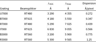
WiFeS grating wavelength ranges and dispersion, as measured from our reduced data. Wavelength limits are rounded to the nearest 5 Å. The beamsplitters are named after their dichroic wavelength split in nanometres. The dispersion and upper wavelength limit for each grating varied over time by less than 0.02%.
Measured throughput of each grating except for U7000 from Dopita et al. (Reference Dopita2010). The shaded region represents the I7000 wavelength bounds in practice (Table 1). The bottom panel shows two examples of spectra that one might fail to measure a redshift from the I7000 grating. For a redshift of $\lesssim$
0.014 (
$\lesssim$
0.014 ( $\gtrsim$
0.065), none of the H
$\gtrsim$
0.065), none of the H $\alpha$
(calcium triplet) region is present in I7000 leaving only weak or no features.
$\alpha$
(calcium triplet) region is present in I7000 leaving only weak or no features.
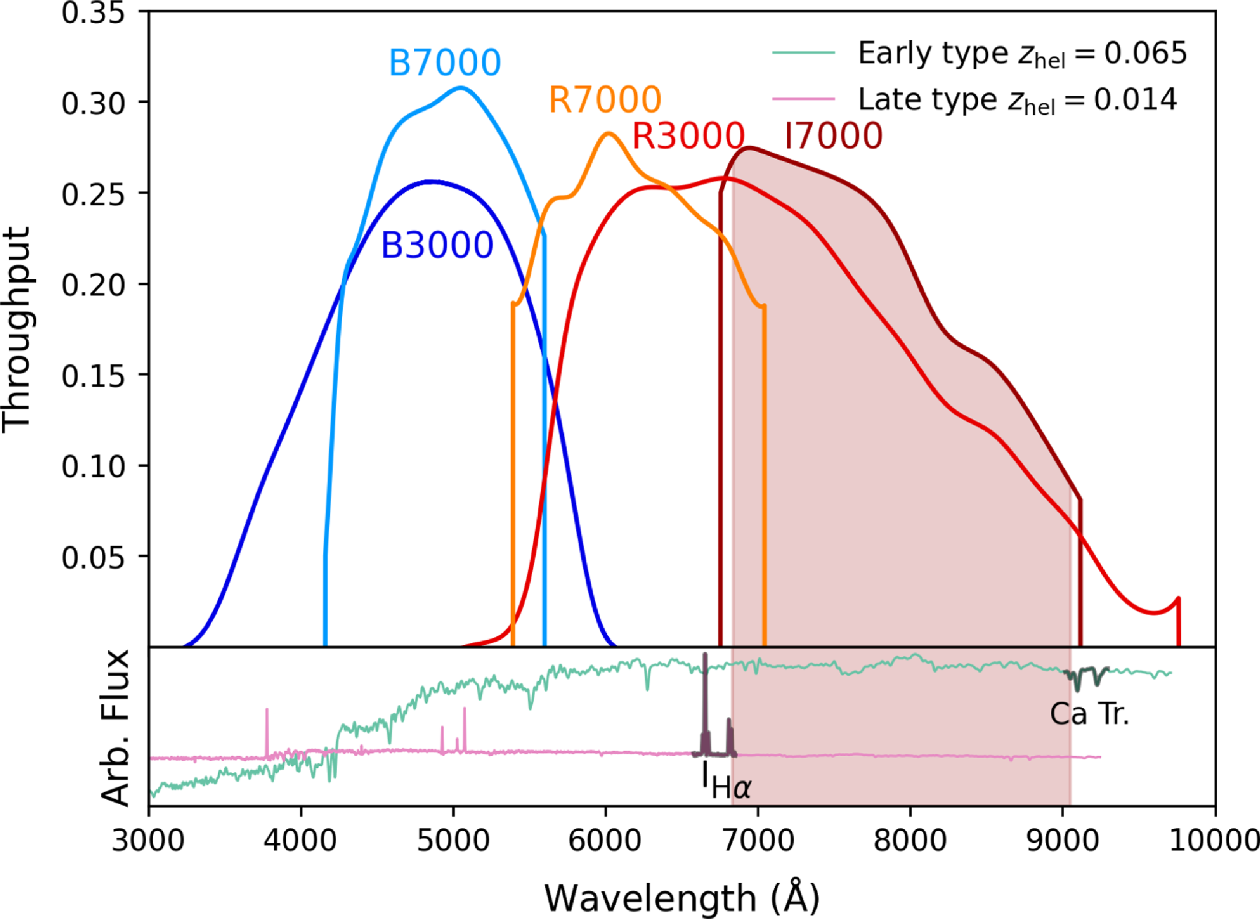
However, after the first two observing runs, we switched to observing with full spectral coverage at $R=3\,000$
, which still offers excellent precision and better S/N for the same exposure time. We made this decision due to the fact that at the low redshifts we were targeting, the I7000 grating was sometimes a trade-off between the calcium triplet and H
$R=3\,000$
, which still offers excellent precision and better S/N for the same exposure time. We made this decision due to the fact that at the low redshifts we were targeting, the I7000 grating was sometimes a trade-off between the calcium triplet and H $\alpha$
region being redshifted out of spectral coverage. We show this in Fig. 1 with two example spectra at redshifts where the I7000 spectral region would be devoid of features. If we have good enough S/N for a late-type galaxy, or the galaxy has a particularly strong calcium triplet, we would still be able to identify features in I7000 below
$\alpha$
region being redshifted out of spectral coverage. We show this in Fig. 1 with two example spectra at redshifts where the I7000 spectral region would be devoid of features. If we have good enough S/N for a late-type galaxy, or the galaxy has a particularly strong calcium triplet, we would still be able to identify features in I7000 below $z\approx 0.014$
, and similar for early-type galaxies above
$z\approx 0.014$
, and similar for early-type galaxies above $z\approx 0.065$
. However, for the final two observation runs, we observed using the B3000+R3000 gratings since they offer full spectral coverage with a generous overlap, and as such have no such restrictions on where typical optical galaxy emission and absorption features land.
$z\approx 0.065$
. However, for the final two observation runs, we observed using the B3000+R3000 gratings since they offer full spectral coverage with a generous overlap, and as such have no such restrictions on where typical optical galaxy emission and absorption features land.
2.2 Target selection
The catalogue was created using the Pantheon supernova sample (Scolnic et al. Reference Scolnic2018) since we conducted all of our observations before the release of Pantheon+. Both the Pantheon and Pantheon+ supernova samples are a vast collection of SNe Ia light curves (1 048 and 1 701, respectively) and redshifts from different sources, both low- and high-z to best constrain cosmology. At the time of observation, Pantheon was the most powerful SN sample, so we aimed to observe as many of the bright, southern SN hosts as possible. Galaxies were chosen to be easily observable from Siding Spring Observatory (latitude $149.06^{\circ}$
, longitude
$149.06^{\circ}$
, longitude $-31.27^{\circ}$
), i.e. airmass
$-31.27^{\circ}$
), i.e. airmass $\lesssim1.5$
, and with
$\lesssim1.5$
, and with $z\lesssim0.1$
as these are the redshifts most influential to
$z\lesssim0.1$
as these are the redshifts most influential to $H_0$
.
$H_0$
.
The strategy was to observe in Nod&Shuffle mode, which results in simultaneous science and sky spectra. The target is exposed on the science CCD pixels, then the telescope is nodded to empty sky and the charge already present is ‘shuffled’ across the CCD so that the sky is exposed on a different set of pixels. Sky subtraction is then just the simple case of subtracting the pure 2D sky spectrum from the observed object+sky 2D spectrum within the same CCD image during data reduction, leaving just the 2D object spectrum. Each galaxy observation was made up of three Nod&Shuffle cycles, with each sky and object exposure being the same length. The sky field was chosen to be as empty as possible, and close by to reduce the time to nod between frames.
Once the targets were chosen, we calculated the rough exposure time using the WiFeS performance calculator.Footnote
a
The aim was a generous S/N of at least 20 in the blue camera after the full 3 $\times$
Nod&Shuffle cycle, which was easily obtained for the brightest galaxies. The red camera naturally gathers more signal for the same observation time, so observation time was optimised for the blue camera. Exposure time depends on the moon phase (all observations were done in grey or dark time), the seeing full width at half maximum (typically 1.6 arcsec at SSO), as well as the airmass and surface brightness of the target. The average total integration time was 485 s for an estimated average g-band surface brightness of 16 mag arcsec
$\times$
Nod&Shuffle cycle, which was easily obtained for the brightest galaxies. The red camera naturally gathers more signal for the same observation time, so observation time was optimised for the blue camera. Exposure time depends on the moon phase (all observations were done in grey or dark time), the seeing full width at half maximum (typically 1.6 arcsec at SSO), as well as the airmass and surface brightness of the target. The average total integration time was 485 s for an estimated average g-band surface brightness of 16 mag arcsec $^{-2}$
. Subexposure times were rounded to the nearest 30 s rather than attempting to save small amounts of time optimising to the nearest second.
$^{-2}$
. Subexposure times were rounded to the nearest 30 s rather than attempting to save small amounts of time optimising to the nearest second.
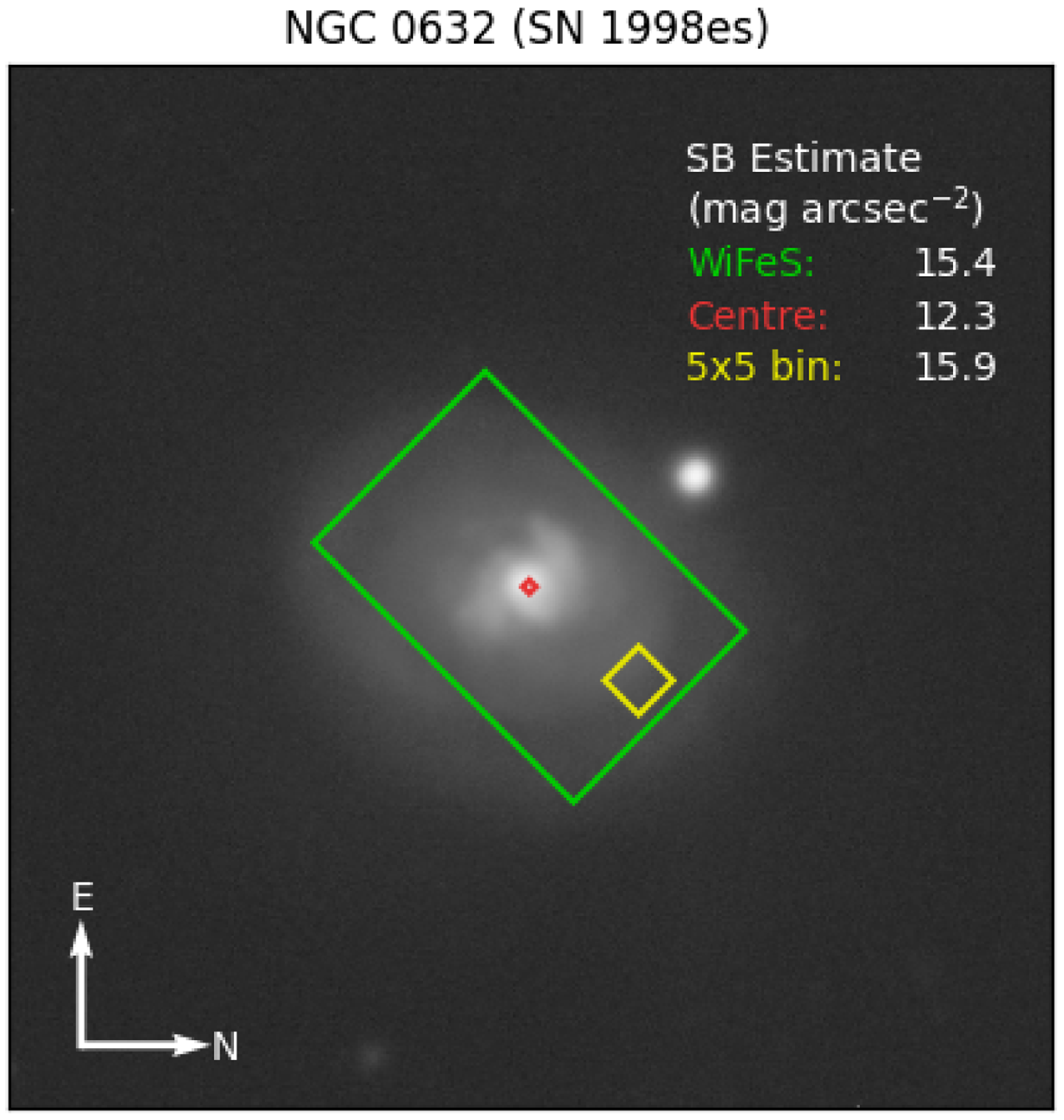
Surface brightness was estimated directly from Dark Energy Camera (DECam) images using the US National Science Foundation’s NOIRLab Astro Data Lab image cutout service.Footnote b Most targets had images; for those that did not, we estimated surface brightness by comparison with similar targets that did have images. When there were images, we opted for sky-subtracted images in the g-band as the highest priority, followed by r-band then i-band (with minor corrections to account for overestimating the g-band magnitude), and stacked images if no sky-subtracted version was available. The surface brightness was estimated from the images using the photutils python packageFootnote c within different apertures, including the full WiFeS aperture, to estimate a useful average for the whole field of view. See Fig. 2 for an example.
DECam g-band image of the galaxy NGC 632, host of SN 1998es. The three estimates of surface brightness were made over the whole WiFeS aperture, within the central pixel of the aperture, and finally, a $5\times 5$
pixel binned aperture on the outskirts to estimate a lower limit of surface brightness.
$5\times 5$
pixel binned aperture on the outskirts to estimate a lower limit of surface brightness.
Flux calibration stars were chosen to be CALSPEC starsFootnote d which are the standards used for the Hubble Space Telescope. The only criterion for choosing a CALSPEC flux calibrator was that it was easily observable from SSO. The CALSPEC standard stars were also used to remove Telluric absorption features from the galaxy spectra. We trialled the use of dedicated, particularly smooth-spectrum Telluric standard stars (hot, main sequence B stars), but were unable to reliably source reference spectra. As such, the Telluric corrections were sometimes lacking, but never resulted in a failure to compute a redshift.
Radial velocity standard stars (stars with well-known radial velocities to compare to as another form of instrument calibration) were chosen from Nidever et al. (Reference Nidever, Marcy, Butler, Fischer and Vogt2002). The stars we used were all chosen to be G- or K-type stars with a preference for giants. They were also chosen to primarily be around $V=6$
mag, similar to the flux calibrators.
$V=6$
mag, similar to the flux calibrators.
Using this strategy, we observed 213 galaxies, 185 of which were unique targets, and the rest duplicates for increased S/N. A log of our observations can be found in Table A1 including MJD of observation and exposure time of our main science targets and radial velocity standards.
2.3 Reduction
We used version 0.7.4 of the default WiFeS reduction pipeline, PyWiFeS (Childress et al. Reference Childress, Vogt, Nielsen and Sharp2014), to transform the raw observations into calibrated, 3D data cubes. In brief, the reduction pipeline pre-processes each CCD image (overscan and bias subtraction, bad pixel repair), then uses spatial calibration frames to split the data into the 25 science and 25 sky slitlets. The instrument was designed so that the sky and science slitlets are interleaved on the detectors, and slitlets lie along detector rows. Over the entire detector, the slitlets deviate from these rows by up to $\sim\pm0.5$
pixels. This deviation is accounted for by observing a uniformly illuminated calibration frame obstructed by a straight wire. The shadow of the wire is used to find the spatial zero-point of each slitlet along the y-direction (the long axis of the aperture) over every CCD column.
$\sim\pm0.5$
pixels. This deviation is accounted for by observing a uniformly illuminated calibration frame obstructed by a straight wire. The shadow of the wire is used to find the spatial zero-point of each slitlet along the y-direction (the long axis of the aperture) over every CCD column.
From here, the usual steps are performed: finding the wavelength solution, cosmic ray rejection, sky-subtraction, flatfielding, flux calibration and Telluric correction. Finally, the data are reformatted to a 3D data cube. We note that while the field of view is $25\times38$
arcsec/spaxels, in practice we trim the noise-dominated outer one or two spaxel rows (depending on the gratings and beamsplitter) so we actually use
$25\times38$
arcsec/spaxels, in practice we trim the noise-dominated outer one or two spaxel rows (depending on the gratings and beamsplitter) so we actually use $25\times35$
spaxels for our purposes.
$25\times35$
spaxels for our purposes.
Due to the excellent stability of the WiFeS instrument, the wavelength solution varied only on the sub-pixel level. We expand upon this in Section 3.
2.4 Spaxel binning and redshift measurement
After reducing the data, the 3D spectral data cube contains a wealth of information. For this work, we are mainly interested in the redshift and its spatial dependence, although there is certainly more that can be done with spatially varying, medium-resolution ( $R=3\,000$
–7 000), high S/N data. To investigate the redshift(s) of the galaxy, we first processed the data further into a format that could be ingested into the Marz redshifting tool,Footnote
e
which was developed primarily for the use of the Australian Dark Energy Survey and Anglo-Australian Telescope, also at SSO.
$R=3\,000$
–7 000), high S/N data. To investigate the redshift(s) of the galaxy, we first processed the data further into a format that could be ingested into the Marz redshifting tool,Footnote
e
which was developed primarily for the use of the Australian Dark Energy Survey and Anglo-Australian Telescope, also at SSO.
To turn our nearly 1 000 individual spaxels into a reasonable number of high S/N spectra, we spatially bin them. This allows us to gather more signal in the outer regions of the aperture, and to successfully measure the redshift of galaxies that occupied very few spaxels. The best tool for the purpose of binning 2D spectroscopic data is the vorbin python package (see Cappellari & Copin Reference Cappellari and Copin2003) which uses Voronoi tessellation to create bins of roughly the target S/N. This adaptive binning method naturally creates a complete tessellation (no overlap or holes) with bins that are as compact as possible (no elongated or fragmented bins) with minimum variation in S/N. This is due to the particular algorithm of seeding, bin-accretion and correction developed by Cappellari & Copin (Reference Cappellari and Copin2003) for the purposes of integral-field spectroscopic data.
See Fig. 3 for a visualisation of how observations are turned into redshifts. It shows the case of a galaxy larger than the aperture, where spaxels further from the bright central region are binned to a common S/N threshold. The redshift of each Voronoi bin is then measured separately. From this map, the average redshift of the whole galaxy, the redshift of the centre and the redshift in the locality of the SN can all be found. The particular example shown does not contain the SN in the aperture; there is only a moderate probability of the SN being within the field of view when centred on such large galaxies.
(a) Image of NGC 6928 on the sky with the WiFeS field of view in green. SN 2004eo occurred outside the green aperture pictured here, nearly one arcminute east-north-east of the centre of the galaxy. (b) S/N over the WiFeS aperture, as averaged per spaxel over the entire red camera spectra. Evidence of the nearby star can be seen as an increase in S/N around spaxel coordinates (25,23), $\sim$
33 arcsec from spaxel (0,0). (c) The Voronoi binning regime that results in each bin having roughly 70% the average S/N of the central spaxel. (d) Final redshift map, showing rotation along the long axis. The average redshift of all the spaxel bins is
$\sim$
33 arcsec from spaxel (0,0). (c) The Voronoi binning regime that results in each bin having roughly 70% the average S/N of the central spaxel. (d) Final redshift map, showing rotation along the long axis. The average redshift of all the spaxel bins is ${z_{\text{hel}}}=0.01576$
, with standard deviation 2.9
${z_{\text{hel}}}=0.01576$
, with standard deviation 2.9 ${\times 10^{-4}}$
. (e) The S/N of each unbinned and binned spaxel, with the dashed line showing the S/N target.
${\times 10^{-4}}$
. (e) The S/N of each unbinned and binned spaxel, with the dashed line showing the S/N target.
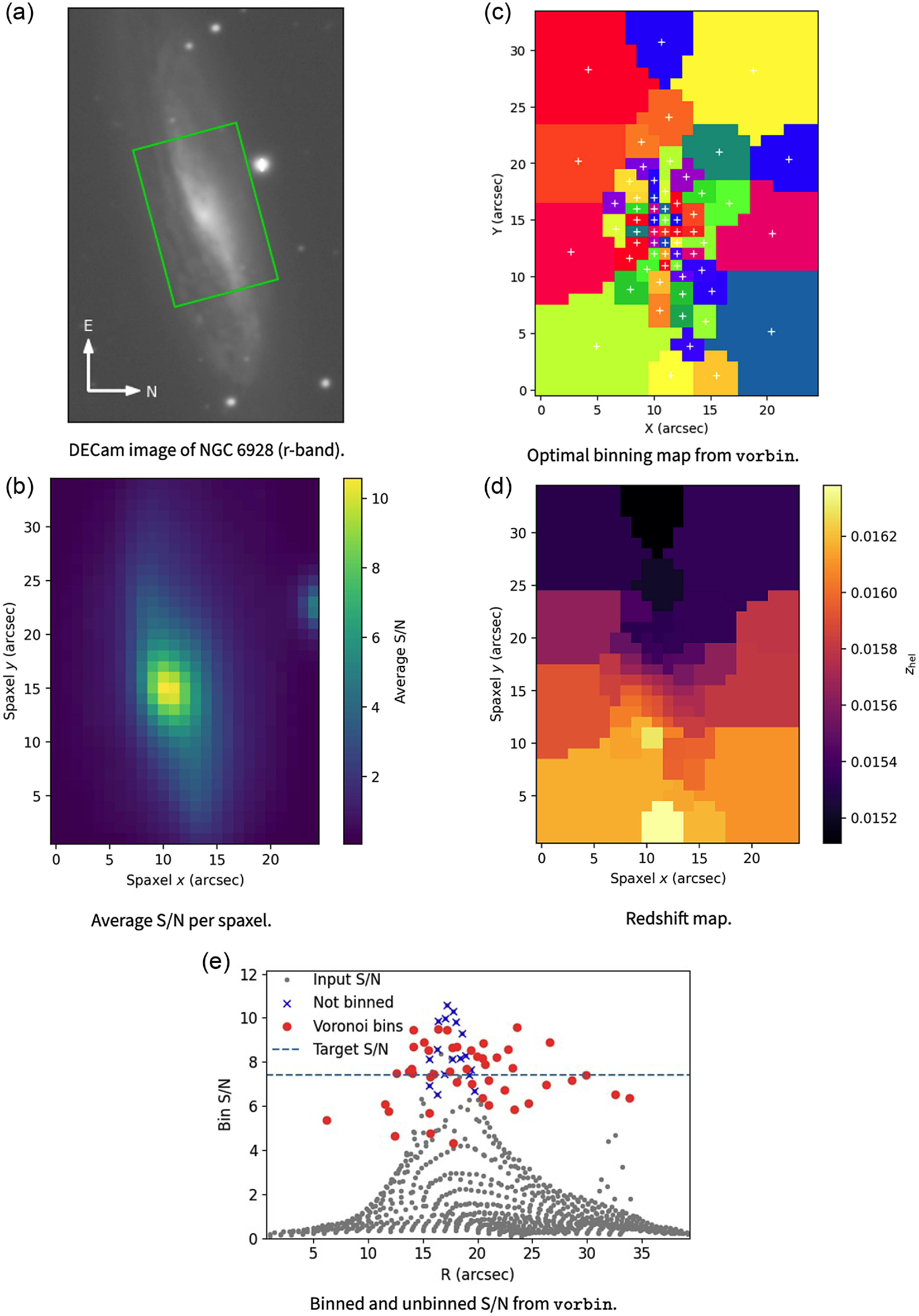
For most of the Voronoi binning, we set the S/N target to 90% of the central pixel S/N by default. This target level was sometimes adjusted in the cases where the surface brightness profile was particularly flat (requiring an increase), such as MCG-02-02-086, the host of SN 2003ic, or the galaxy as a whole was extremely bright (requiring a decrease to reduce the number of bins from $\gg$
100 to
$\gg$
100 to $\lesssim$
100), such as NGC 6928, featured in Fig. 3. In each case, the binning was visually inspected to ensure both a decent number of bins and high-quality spectra for each.
$\lesssim$
100), such as NGC 6928, featured in Fig. 3. In each case, the binning was visually inspected to ensure both a decent number of bins and high-quality spectra for each.
In 24 cases, there was only one bin, necessary for the particularly small/faint/poor-quality-spectrum galaxies to successfully obtain an accurate redshift. Where possible, we also redshift just the central region (estimated from the highest S/N spaxels), to compare with the average redshift over all Voronoi bins. This often resulted in a strong increase in S/N; however, for the 24 cases above, a similar or lower S/N spectrum naturally resulted, since we did not use as many spaxels as for the whole galaxy. Of the 185 galaxies we observed, 106 were at least roughly as large in the sky as the aperture, and nine were small enough to occupy only several spaxels each. For the standard stars, the $3\times 3$
spaxel region around the centre of the star was used for measuring redshift.
$3\times 3$
spaxel region around the centre of the star was used for measuring redshift.
The geocentric-to-heliocentric correction to account for our motion around the Sun is automatically handled in Marz by including the relevant headers for the telescope location, observation time, and object coordinates. The distribution of geocentric corrections between $-25$
and
$-25$
and $+20$
km s
$+20$
km s $^{-1}$
only had a slight positive gradient; however, the mean correction was 11.7 km s
$^{-1}$
only had a slight positive gradient; however, the mean correction was 11.7 km s $^{-1}$
due to a large number of corrections falling between
$^{-1}$
due to a large number of corrections falling between $+20$
and
$+20$
and $+30$
km s
$+30$
km s $^{-1}$
.
$^{-1}$
.
3. Instrument throughput correction
Transforming the data from photon counts to accurate flux as a function of accurate wavelength is a multi-step process. ‘Dome’ flats using an internal Quartz-Iodine lamp correct for the CCD pixel-to-pixel quantum efficiency. The Quartz-Iodine lamp is mostly ‘spectrally flat’, in that the wavelength dependence can be removed by a moderate order polynomial, but does not illuminate the instrument perfectly uniformly. Twilight flats using the twilit sky (which are ‘spatially’ flat, i.e. uniform illumination, but significant spectral deviation) are used to correct for the spatial illumination. Once the pixel-to-pixel and large-scale illumination are corrected, one of the final steps is flux calibration, which corrects for the wavelength response and instrument+atmosphere throughput.
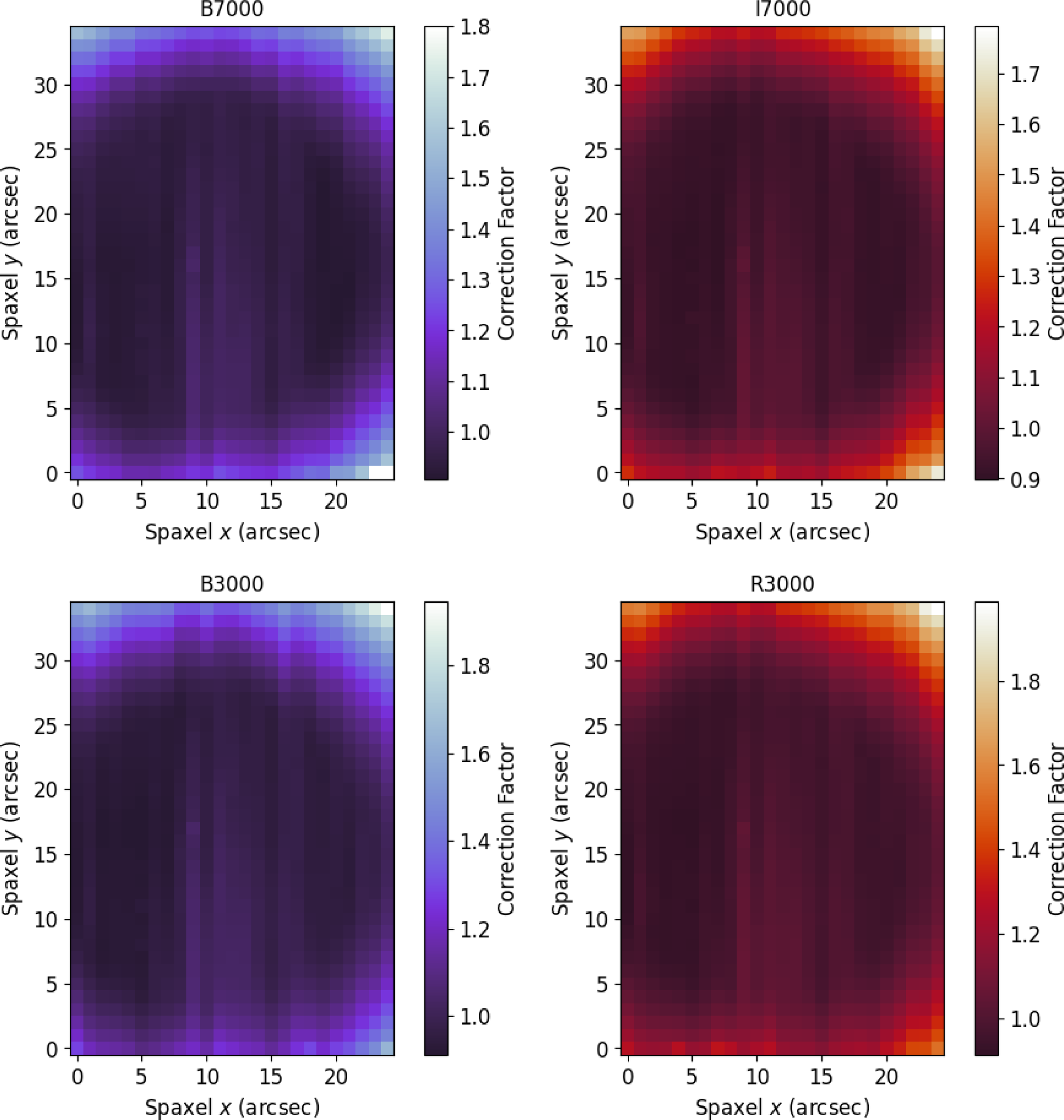
Childress et al. (Reference Childress2016) studied the performance of the WiFeS instrument over a three-year period for the ANU WiFeS SuperNovA Programme (AWSNAP), including wavelength solution, illumination correction, and flux calibration. We have a similar set of data gathered over a year in two operation modes, five years later, with which to compare. We emulate their analysis here to observe any trends over nightly to yearly scales and detect any need for manual recalibration. We start by examining the illumination correction for our different operating modes (see Fig. 4) and find no significant differences (visually) between them and Childress et al. (Reference Childress2016), which speaks to the stability of the instrument.
Illumination corrections for the red and blue camera averaged over each observation run in each operation mode, as determined from twilight flats (see text). The $R=3\,000$
and
$R=3\,000$
and $R=7\,000$
grating corrections are basically the same since this is a spatial correction. The corrections are also comparable to those of Childress et al. (Reference Childress2016) indicating the stability of the instrument over several years.
$R=7\,000$
grating corrections are basically the same since this is a spatial correction. The corrections are also comparable to those of Childress et al. (Reference Childress2016) indicating the stability of the instrument over several years.
4. Wavelength calibration methods
In this section, we study the accuracy of the instrument so we can be assured the redshifts we measure are not biased. We study the effects of temperature fluctuation on the wavelength solution throughout each night and over the entire observation program in Section 4.1. We also use the skylines that we measure simultaneously with our science targets to track how the wavelength solution varies across the aperture in Section 4.2. Finally, in Section 4.3, we compare our redshift measurements of radial velocity standard stars to their accurately known values, along with the effects of the spectral template we use to measure redshift. In essence, we find that the wavelength solution shows excellent stability and thus our redshifts require no spatial or temperature correction.
4.1 Arc lamp wavelength solutions and temperature dependence
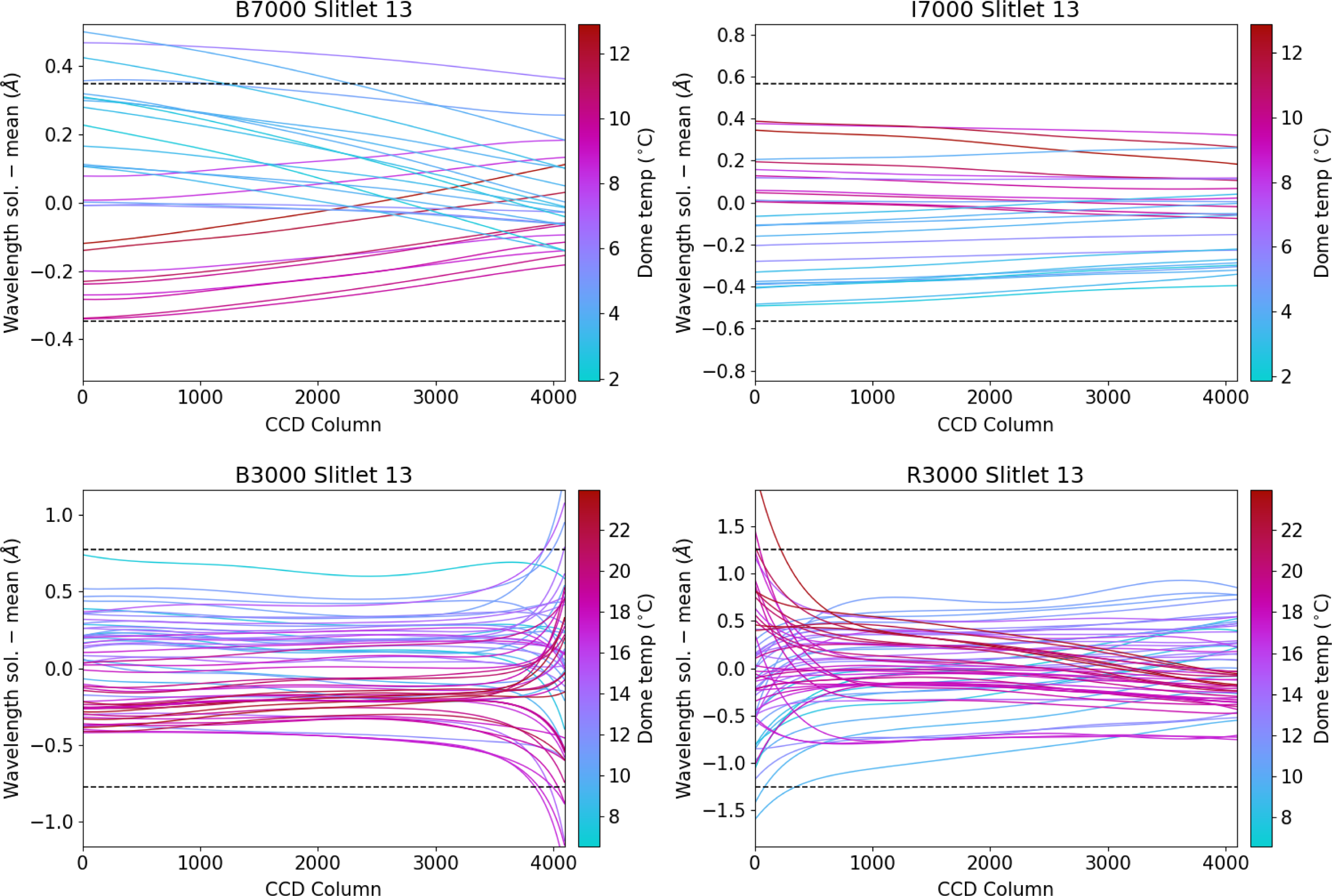
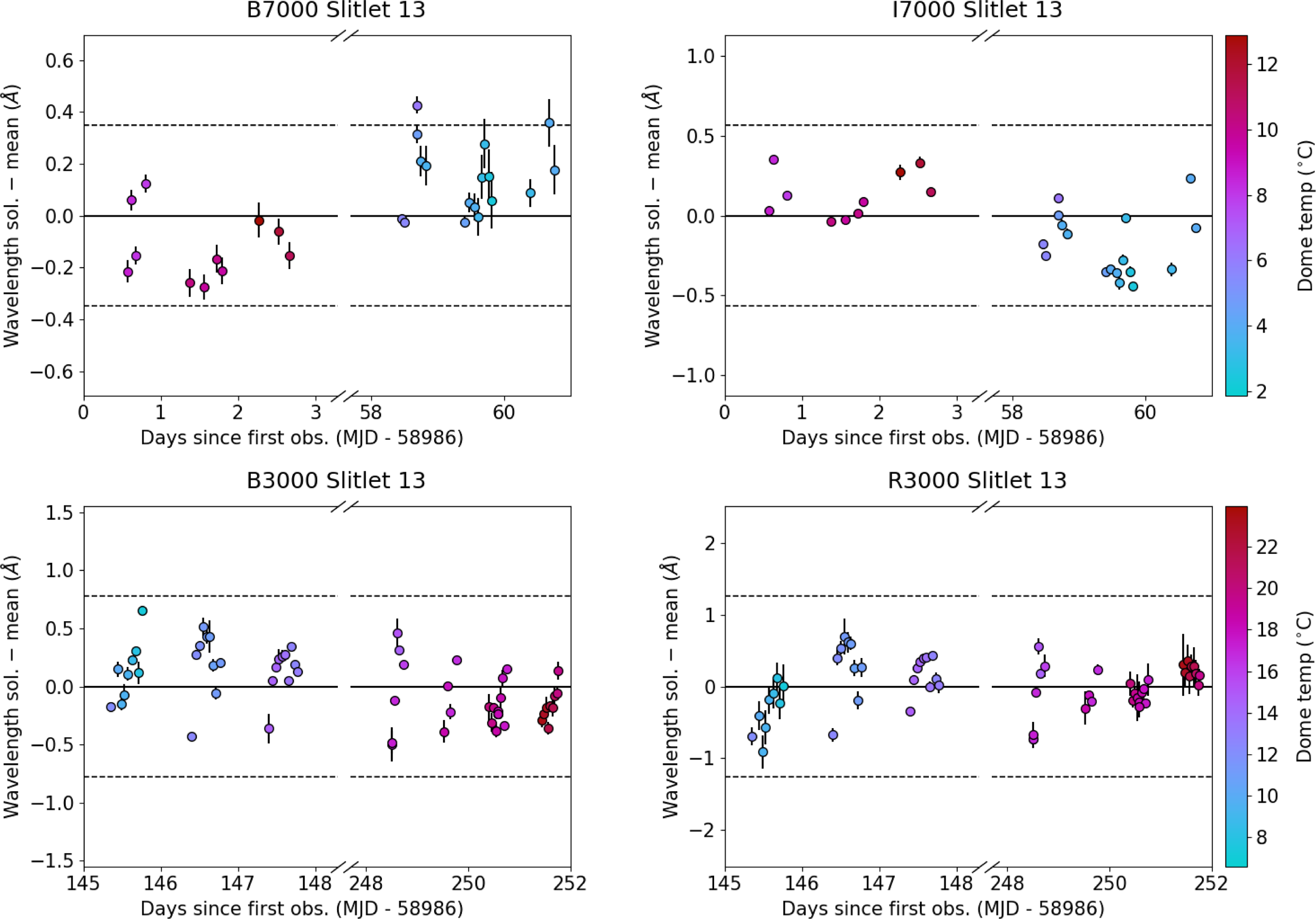
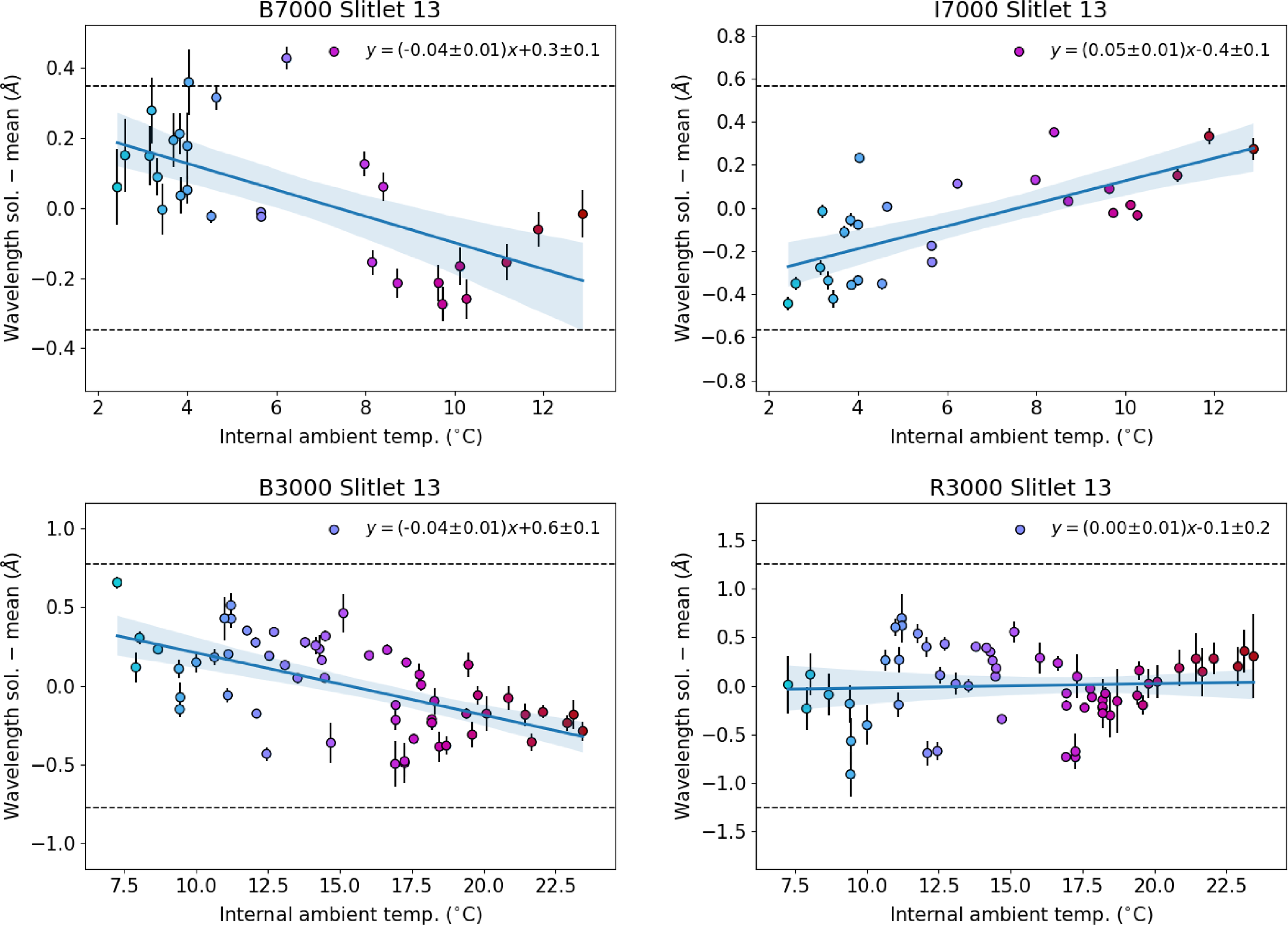
It is well known that temperature fluctuations inside the dome affect the wavelength solution of WiFeS spectra, as the gratings themselves thermally expand. We endeavoured to mitigate any temperature effects by taking frequent arc lamp calibration frames. The response of the gratings to temperature fluctuations may be linear, which can be interpolated over easily, but the temperature fluctuations themselves are not and lag behind the dome internal temperature readings. By making frequent arc lamp observations, temperature variations are accounted for since each science observation is calibrated using the nearest arc lamp in time, or if the science observation falls between two arc lamps, it is calibrated by the average of those wavelength solutions. Similar to Childress et al. (Reference Childress2016), we investigated the variation of the wavelength solution over the CCD, and over time, and we compare both of these to dome temperature readings to correlate with the fluctuations.
Figs. 5–7. show our investigation into wavelength solution variation as measured from arc lamp observations. Over our entire observation program that spanned one year, we used two different resolutions each for two runs (approximately spanning 6 months each). We find very similar results to Childress et al. (Reference Childress2016), in that the average wavelength solution generally deviates by $\pm 0.5$
Å which for our gratings is always less than a CCD pixel (see Table 1), except for a couple of B7000 measurements. There are no long-term trends (albeit with only a single year of data) apart from the seasonal (temperature) difference. Even extreme temperature fluctuations are expected to cause an order
$\pm 0.5$
Å which for our gratings is always less than a CCD pixel (see Table 1), except for a couple of B7000 measurements. There are no long-term trends (albeit with only a single year of data) apart from the seasonal (temperature) difference. Even extreme temperature fluctuations are expected to cause an order $\sim1$
Å fluctuation in wavelength solution.
$\sim1$
Å fluctuation in wavelength solution.
Difference in the wavelength solution over the CCD for each resolution and camera, compared to the mean for that resolution+camera combination. We show only the middle slitlet, but the others show similar overall trends (see Childress et al. Reference Childress2016). Each curve is a different arc lamp observation, coloured by the temperature recorded at that time. The dashed lines denote the size of a CCD pixel. $R=7\,000$
shows similar levels of variation to
$R=7\,000$
shows similar levels of variation to $R=3\,000$
(despite the differing wavelength dispersions), except at the CCD column boundary, where the variation is less extreme because a) throughput is higher at higher resolution (especially toward the ends of wavelength coverage where B3000 and R3000 drop to near 0; see Fig. 1), and b) the wavelength solution for
$R=3\,000$
(despite the differing wavelength dispersions), except at the CCD column boundary, where the variation is less extreme because a) throughput is higher at higher resolution (especially toward the ends of wavelength coverage where B3000 and R3000 drop to near 0; see Fig. 1), and b) the wavelength solution for $R=3\,000$
gratings is less stable in the dichroic region at high (low) CCD column numbers for B3000 (R300).
$R=3\,000$
gratings is less stable in the dichroic region at high (low) CCD column numbers for B3000 (R300).
The same as Fig. 5 but now averaged across the CCD column and as a function of observation date. The dependence on temperature is still clear, but now the seasonal dependence is seen by the grouping in different observation runs.
Average difference in wavelength solution as a function of temperature. The colour map is carried through from Figs. 5 and 6, i.e. the x-axis here. Since we observed for a full year, our observations roughly capture the extremes of temperature during a typical year, so it is expected that the average wavelength solution will not vary by more than a CCD pixel. According to the linear relations fit to the temperature data, even if the temperature does vary more than expected, it would still be predominantly sub-pixel.
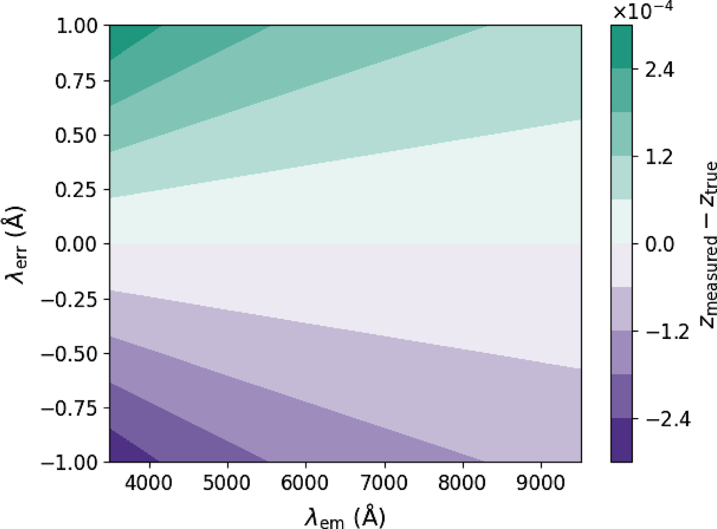
To put into perspective how a 1 Å error would appear when measuring a redshift, we show in Fig. 8 the severity of measuring a spectral feature up to $\pm$
1 Å off its true value for a source
$\pm$
1 Å off its true value for a source $z=0.1$
,Footnote
f
over the full spectral range of WiFeS. The error is more severe at the blue end, but we generally use features in the red for measuring redshift. Over the entire CCD, the average temperature-induced shift is less than 0.5 Å which we account for with frequent calibration, so the expected temperature-induced redshift error is much less than the maximum
$z=0.1$
,Footnote
f
over the full spectral range of WiFeS. The error is more severe at the blue end, but we generally use features in the red for measuring redshift. Over the entire CCD, the average temperature-induced shift is less than 0.5 Å which we account for with frequent calibration, so the expected temperature-induced redshift error is much less than the maximum $\sim0.5$
Å or redshift of
$\sim0.5$
Å or redshift of $\sim6{\times 10^{-5}}$
from Fig. 8. Below, we show that when we redshift well-known objects/features, we indeed see a smaller average error.
$\sim6{\times 10^{-5}}$
from Fig. 8. Below, we show that when we redshift well-known objects/features, we indeed see a smaller average error.
4.2 Skylines
Skylines are strong emission lines, mostly in infrared, that come from our own atmosphere and need to be removed from our spectra. However, since they originate on Earth, we can use them as a test of wavelength solution in addition to arc lamps. For every science target, we measured the ‘redshift’ of the sky spectrum (which is coincident with but separate from the science spectra due to the Nod&Shuffle mode of operation) in the centre and corners of the aperture to test how the wavelength solution varied across the field of view. For a small subset of the entire science sample (one observation from every night), we did the same without any binning, i.e. we tested the wavelength solution of every spaxel since the S/N of the individual skylines is always very high. To get the redshift of a sky spectrum, we modified Marz to use a high S/N sky spectrum from the European Southern Observatory’s skycorr tool (Noll et al. Reference Noll2014) as a template. Fig. 9 shows the average wavelength solution across the aperture, grouped by resolution. The $R=3\,000$
gratings show more variation, but each only varies by
$R=3\,000$
gratings show more variation, but each only varies by $ \lt 5{\times 10^{-5}}$
, and the central region is always accurate to within
$ \lt 5{\times 10^{-5}}$
, and the central region is always accurate to within $\pm2{\times 10^{-5}}$
.
$\pm2{\times 10^{-5}}$
.
Fig. 10 shows the results of binning the central and outer regions separately for the high and low-resolution configurations. The $R=7\,000$
gratings show little variability, especially in the centre. In every case, the mean offset is
$R=7\,000$
gratings show little variability, especially in the centre. In every case, the mean offset is $ \lt 2{\times 10^{-5}}$
, which corresponds to
$ \lt 2{\times 10^{-5}}$
, which corresponds to $ \lt 0.1$
Å in our observable skyline spectral region (much less than any grating’s resolution).
$ \lt 0.1$
Å in our observable skyline spectral region (much less than any grating’s resolution).
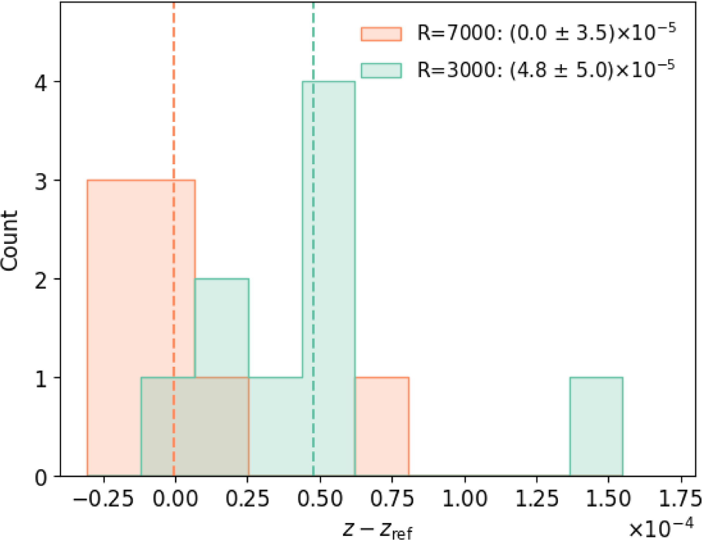
4.3 Radial velocity standards
As a final test of the wavelength solution, we also observed radial velocity standard stars. The radial velocities of these stars are known precisely (Nidever et al. Reference Nidever, Marcy, Butler, Fischer and Vogt2002), so we can compare wavelength solution in a similar way to the known zero-redshift wavelength of skylines. Fig. 11 shows the redshift difference of each observation of a radial velocity standard (some observations are of the same star on different nights), split by resolution mode. As expected, $R=7\,000$
is much more precise, with an undetectable redshift bias, whereas
$R=7\,000$
is much more precise, with an undetectable redshift bias, whereas $R=3\,000$
has an offset of
$R=3\,000$
has an offset of $5{\times 10^{-5}}$
. Both sets have
$5{\times 10^{-5}}$
. Both sets have $ \lt 10$
observations so it is hard to conclude if there is any meaningful correction that needs to be made to the redshifts we obtain for other targets. Both sets are also skewed by a large outlier. When we investigated the outlier, we found that the arc lamp frame used to calibrate the spectrum notably influenced the redshift and that the observation
$ \lt 10$
observations so it is hard to conclude if there is any meaningful correction that needs to be made to the redshifts we obtain for other targets. Both sets are also skewed by a large outlier. When we investigated the outlier, we found that the arc lamp frame used to calibrate the spectrum notably influenced the redshift and that the observation $\sim$
0.5 h after astronomical twilight differed in measured redshift by 7
$\sim$
0.5 h after astronomical twilight differed in measured redshift by 7 ${\times 10^{-5}}$
from the observation
${\times 10^{-5}}$
from the observation $\sim$
2.5 h after twilight. These two effects are seemingly unrelated, however, so this is an interesting example of how observing conditions may have unaccounted effects on redshifts.
$\sim$
2.5 h after twilight. These two effects are seemingly unrelated, however, so this is an interesting example of how observing conditions may have unaccounted effects on redshifts.
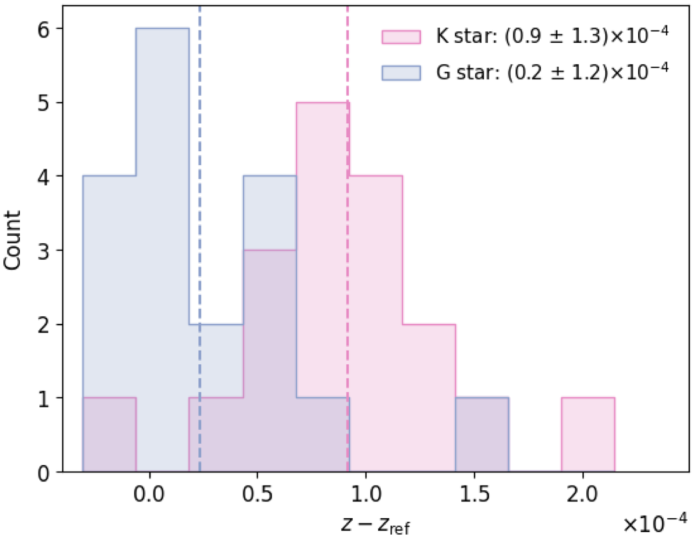
All the radial velocity standards we chose were spectral type G or K, so we also tested how the stellar template used affected the redshift, regardless of the actual spectral type. Thus we measured the redshift of each star with both a G and a K-star template in Marz. Fig. 12 shows the difference in redshift offset when each template was used. Note that we now make no distinction between resolution, and the G template histogram is exactly the combined distribution of Fig. 11. Interestingly, the K-star template resulted in moderately biased redshifts, by $+7{\times 10^{-5}}$
, even if the star was itself K-type.
$+7{\times 10^{-5}}$
, even if the star was itself K-type.
Naïvely, the best solution should be to measure the redshift of a star with the closest-matching spectral type template. However, one would also expect these two templates, in particular, to agree since the absorption features are similar for K and G. The difference between the two templates in Marz is that the G template covers a broader wavelength range than K and includes the calcium triplet. Assuming the broader wavelength coverage of the G-type stellar template is the main reason for the disagreement, we opted to measure the redshift of all the radial velocity standards with this template. In addition, our redshifts from the G-star template show better agreement with the published radial velocities in every case.
Apart from this moderate disagreement between stellar templates, none of our investigations into the accuracy of our wavelength solution revealed any need to further calibrate our redshifts. The stellar template problem is interesting and may require further investigation, although in the case of galaxies, it remains important to measure redshifts with the template that best matches. The redshift of a high S/N galaxy spectrum can be measured using an early, intermediate or late-type template, but the redshift may shift up to a couple of ${10^{-4}}$
depending on which main features the target and template galaxy displays. As such, we always redshift galaxies with their matching template in Marz.
${10^{-4}}$
depending on which main features the target and template galaxy displays. As such, we always redshift galaxies with their matching template in Marz.
From our investigations, we are assured our redshifts are accurate to within several ${10^{-5}}$
.
${10^{-5}}$
.
5. Results
We assess the success of our redshift program predominantly by estimating how accurate and precise our measurements are. We studied the accuracy of the instrument in Section 4, so here we compare our redshifts measured from two different binning regimes (averaging over the aperture and measuring just the core) to confirm we are not biased by pointing or galaxy rotation, and we also provide a comparison to the Pantheon+ sample in Section 5.1. We study the precision of our survey in Section 5.2 by generating many realisations of our spectra based on their measured noise and isolating individual spectral feature redshifts. Importantly, we check how our redshifts affect cosmology in Section 5.3, as we specifically targeted galaxies that have the greatest potential to shift $H_0$
.
$H_0$
.
The redshift error resulting from measuring a spectral feature at $\lambda_{\mathrm{em}}$
up to
$\lambda_{\mathrm{em}}$
up to $\pm$
1 Å (
$\pm$
1 Å ( $\lambda_{\mathrm{err}}$
) from its true value, due to, e.g. a small residual temperature dependence in the wavelength solution. We generally redshift features in the red (H
$\lambda_{\mathrm{err}}$
) from its true value, due to, e.g. a small residual temperature dependence in the wavelength solution. We generally redshift features in the red (H $\alpha$
, Ca triplet), and the average wavelength solution error is less than 0.5 Å over most of the CCD (Fig. 5), resulting in a realistic maximum redshift error of
$\alpha$
, Ca triplet), and the average wavelength solution error is less than 0.5 Å over most of the CCD (Fig. 5), resulting in a realistic maximum redshift error of $\sim6{\times 10^{-5}}$
. Sources whose features are primarily at low wavelengths could potentially experience larger errors.
$\sim6{\times 10^{-5}}$
. Sources whose features are primarily at low wavelengths could potentially experience larger errors.
5.1 Redshift performance and comparison
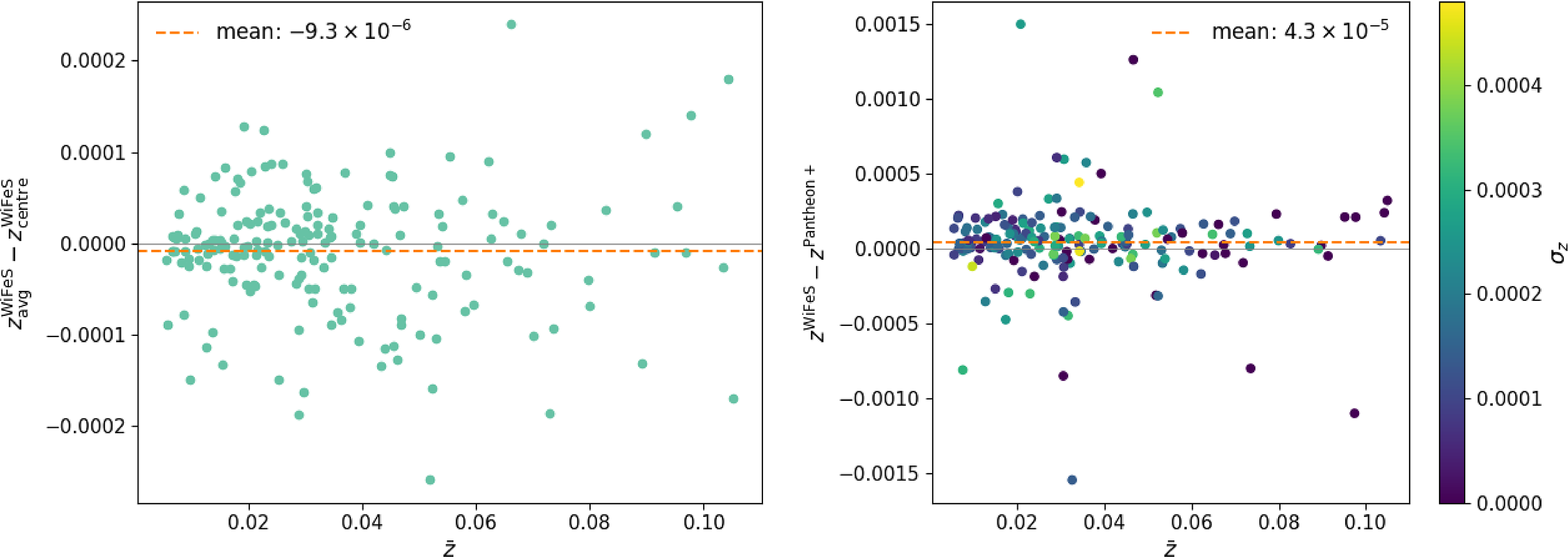
Most galaxies (161/185) are bright and large enough in the sky to obtain at least one redshift at different spatial locations with which we can characterise the average redshift. Others (24/185), however, were too small, dim, or otherwise had too little S/N to obtain multiple redshifts, so instead the redshift was measured using the entire spatial extent of the galaxy. The average redshift also reflects the systemic redshift of the galaxy provided that the aperture was centred on the galaxy. Since this is not always the case, we also measure the redshift of just the core section of the galaxy, where possible, to compare to. This comparison is shown in Fig. 13. The mean offset is $-9.3{\times 10^{-6}}$
, and the scatter is of the order of several
$-9.3{\times 10^{-6}}$
, and the scatter is of the order of several ${10^{-5}}$
. The agreement on average is as good as we can expect given our investigations into the accuracy of the wavelength solution, but the scatter is also affected by whether the galaxy was centred in the aperture, the S/N, and whether the galaxy was early or late-type (roughly absorption or emission features predominantly being displayed, respectively). The last two effects are discussed in Section 5.2 regarding the redshift variation we might expect to see when measuring redshift from high/low S/N or narrow/wide absorption or emission features. The largest outlier is the host of SN 2009Y, NGC 5728, which has very strongly double-peaked emission lines, even in the central region. In this case, using the Ca triplet to measure the redshift is much preferred, but it was not always present with high S/N.
${10^{-5}}$
. The agreement on average is as good as we can expect given our investigations into the accuracy of the wavelength solution, but the scatter is also affected by whether the galaxy was centred in the aperture, the S/N, and whether the galaxy was early or late-type (roughly absorption or emission features predominantly being displayed, respectively). The last two effects are discussed in Section 5.2 regarding the redshift variation we might expect to see when measuring redshift from high/low S/N or narrow/wide absorption or emission features. The largest outlier is the host of SN 2009Y, NGC 5728, which has very strongly double-peaked emission lines, even in the central region. In this case, using the Ca triplet to measure the redshift is much preferred, but it was not always present with high S/N.
We present our redshifts in Table A2 and Fig. 13. We find a mean systematic offset of 4.3 ${\times 10^{-5}}$
with normalised median absolute deviation (NMAD) of 1.2
${\times 10^{-5}}$
with normalised median absolute deviation (NMAD) of 1.2 ${\times 10^{-4}}$
between our redshifts and Pantheon+, which, as shown by Carr et al. (Reference Carr2022) is negligible for SN cosmology. However, surprisingly, there are several redshift discrepancies above the level of
${\times 10^{-4}}$
between our redshifts and Pantheon+, which, as shown by Carr et al. (Reference Carr2022) is negligible for SN cosmology. However, surprisingly, there are several redshift discrepancies above the level of ${10^{-3}}$
, and we show the two largest in Fig. 14. Neither of these examples came from optical host galaxy spectra.
${10^{-3}}$
, and we show the two largest in Fig. 14. Neither of these examples came from optical host galaxy spectra.
Wavelength solution (effectively redshift) calibration across the aperture per grating, found by means of measuring the ‘redshift’ of the $z=0$
sky spectrum, with no spatial binning.
$z=0$
sky spectrum, with no spatial binning.
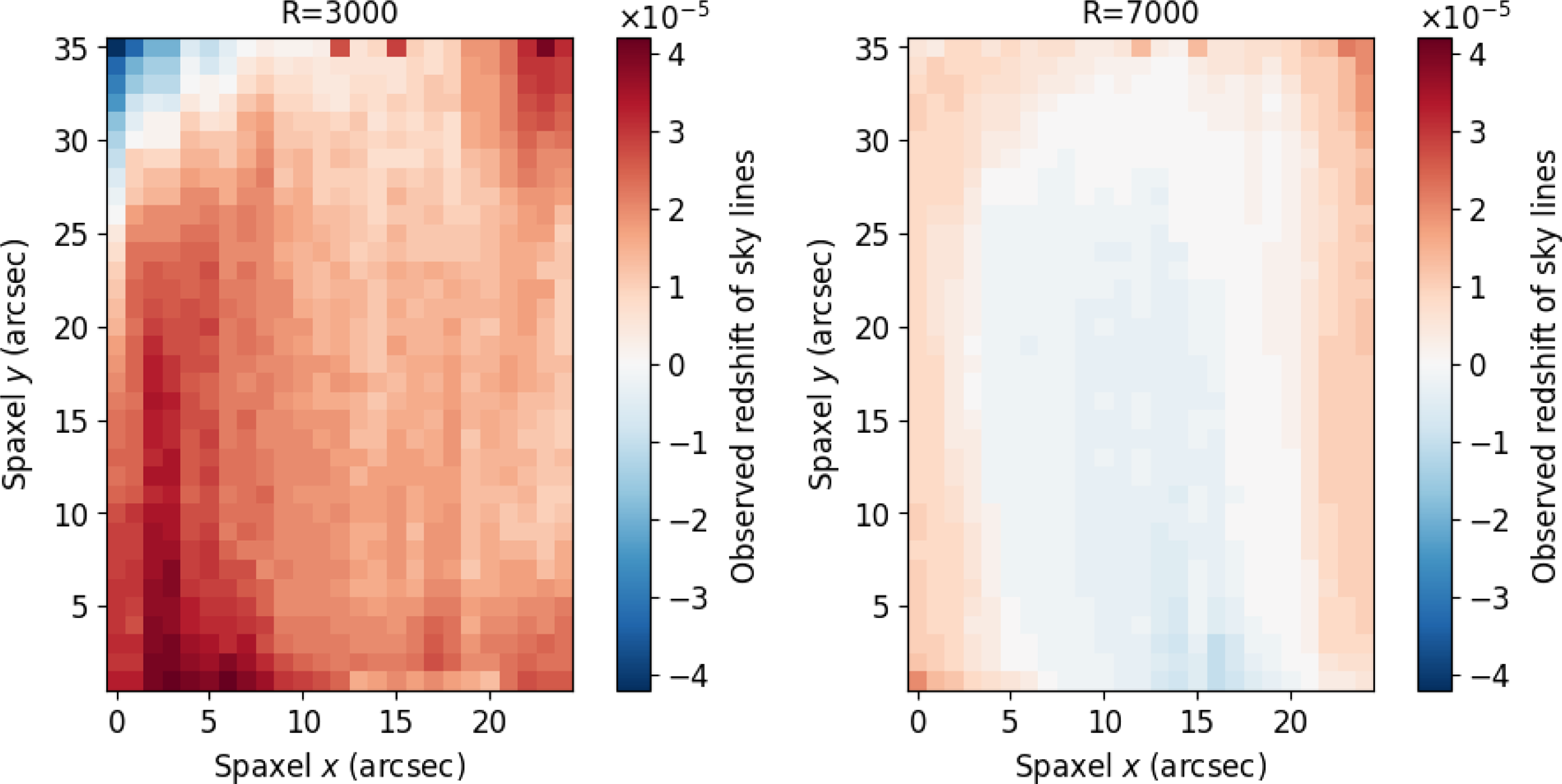
Wavelength solution/redshift calibration across the aperture with binning shown in the upper right of each panel, from the observed redshift of the $z=0$
sky spectrum. The left panel shows
$z=0$
sky spectrum. The left panel shows $R=3\,000$
and the right panel shows
$R=3\,000$
and the right panel shows $R=7\,000$
. These curves have been smoothed over the
$R=7\,000$
. These curves have been smoothed over the $\sim$
200 sky-spectrum observations for each individual aperture region. The double-peaked nature of the
$\sim$
200 sky-spectrum observations for each individual aperture region. The double-peaked nature of the $R=3\,000$
curve for the outer regions comes from the fact that the upper left corner is generally blueshifted, and the upper right and lower left redshifted from the centre (see Fig. 9). This is also the case for
$R=3\,000$
curve for the outer regions comes from the fact that the upper left corner is generally blueshifted, and the upper right and lower left redshifted from the centre (see Fig. 9). This is also the case for $R=7\,000$
but to a much lesser extent.
$R=7\,000$
but to a much lesser extent.
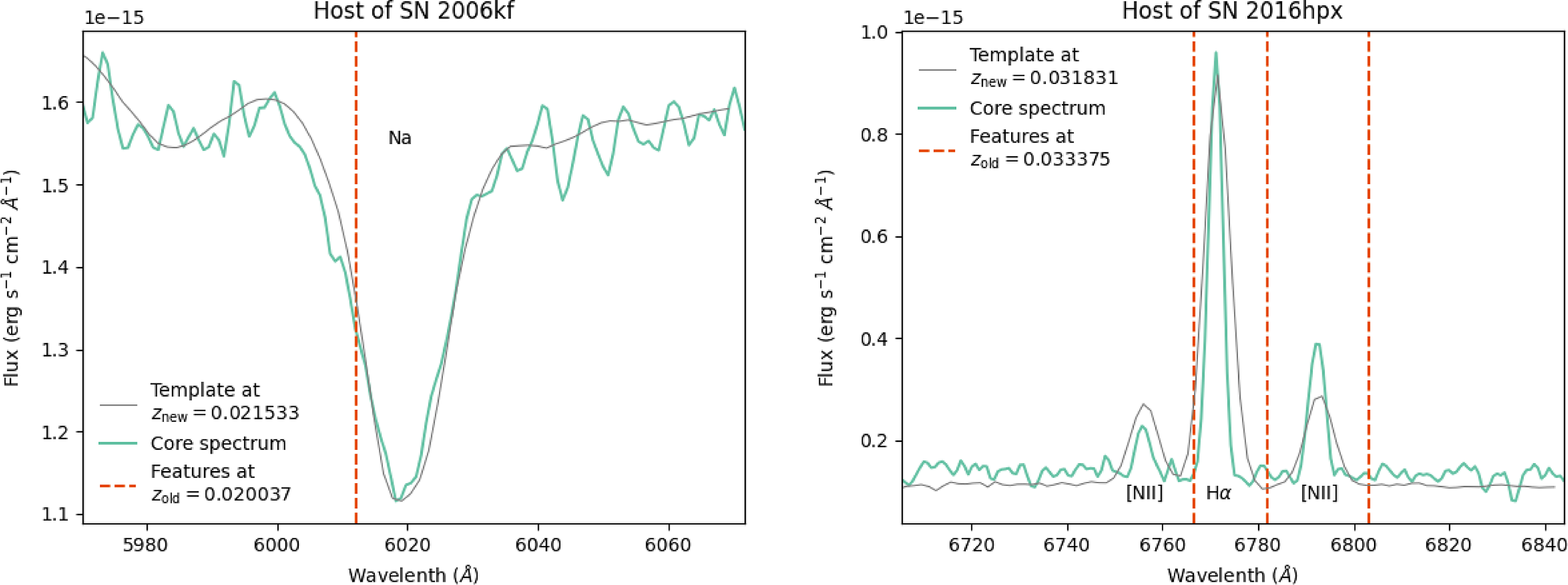
For SN 2006kf, the original redshift, $z_{\text{old}}=0.020037$
came from a single-peaked 21 cm profile according to the NASA/ IPAC Extragalactic Database,Footnote
g
in contrast to our measurement of
$z_{\text{old}}=0.020037$
came from a single-peaked 21 cm profile according to the NASA/ IPAC Extragalactic Database,Footnote
g
in contrast to our measurement of $z=0.021533$
(a difference of
$z=0.021533$
(a difference of $1.5{\times 10^{-3}}$
). A low S/N double horn distribution could potentially be mistaken for a single horn, and therefore could bias the redshift determination by the rotation of the galaxy.
$1.5{\times 10^{-3}}$
). A low S/N double horn distribution could potentially be mistaken for a single horn, and therefore could bias the redshift determination by the rotation of the galaxy.
For SN 2016hpx, the original redshift $z_{\text{old}}=0.033375$
was measured from the publicly available SN classification spectrum which showed possible host galaxy H
$z_{\text{old}}=0.033375$
was measured from the publicly available SN classification spectrum which showed possible host galaxy H $\alpha$
emission (Foley et al. Reference Foley2018; Dimitriadis et al. Reference Dimitriadis2016). Of the two publicly available reductions of the same spectrum on the Weizmann Interactive Supernova Data RepositoryFootnote
h
(WISeREP), one does indeed show a faint peak in the wavelength region that would be consistent with a host galaxy around
$\alpha$
emission (Foley et al. Reference Foley2018; Dimitriadis et al. Reference Dimitriadis2016). Of the two publicly available reductions of the same spectrum on the Weizmann Interactive Supernova Data RepositoryFootnote
h
(WISeREP), one does indeed show a faint peak in the wavelength region that would be consistent with a host galaxy around $z=0.033$
; however, the other does not. This could be a chance detection of a faint emission line, but it is only a single, weak feature and the spectra are low resolution and quality. The discrepancy with our measurement of
$z=0.033$
; however, the other does not. This could be a chance detection of a faint emission line, but it is only a single, weak feature and the spectra are low resolution and quality. The discrepancy with our measurement of $z=0.031831$
(a difference of
$z=0.031831$
(a difference of $1.5{\times 10^{-3}}$
) would be consistent with the original redshift being mistaken as it is not a case of galactic rotation since the host, LEDA 762493, is almost face-on and the SN occurred only
$1.5{\times 10^{-3}}$
) would be consistent with the original redshift being mistaken as it is not a case of galactic rotation since the host, LEDA 762493, is almost face-on and the SN occurred only $3^{\prime\prime}$
from the core.
$3^{\prime\prime}$
from the core.
Intriguingly, the magnitude of the offset with Pantheon+ is almost exactly that of the average geocentric correction of 11.7 km s $^{-1}$
(
$^{-1}$
( $z=3.9{\times 10^{-5}}$
) we apply to our redshifts. Since the offset is so small, the most likely reason we see it is just due to chance. Perhaps it could imply that the historical redshifts from Pantheon+ did not have a geocentric correction applied, but this is difficult to test, as it requires the exact observation location and time. In any case, the individual large redshift discrepancies are potentially more interesting than this small systematic offset.
$z=3.9{\times 10^{-5}}$
) we apply to our redshifts. Since the offset is so small, the most likely reason we see it is just due to chance. Perhaps it could imply that the historical redshifts from Pantheon+ did not have a geocentric correction applied, but this is difficult to test, as it requires the exact observation location and time. In any case, the individual large redshift discrepancies are potentially more interesting than this small systematic offset.
Redshift offset from our observations compared to the published radial velocities of radial velocity standards. Again the higher resolution performs better, but both suffer from a large positive outlier.
Redshift offset of all radial velocity standards regardless of resolution, but with redshift measured using different stellar templates in Marz. There is a disparity between the average redshift as measured by each template spectral type.
Left: Self-consistency between the average redshift over all Voronoi spaxel bins in each galaxy and just the core section. Right: Difference in the redshift of each galaxy as averaged over all spaxel bins from WiFeS (this work) and Pantheon+, coloured by the standard deviation in redshift over each spaxel bin within each galaxy. The mean offset is 4.3 ${\times 10^{-5}}$
, and insensitive to the outliers, which are interesting in themselves. The mean offset is similar in both panels, but the scatter in the self-consistency check in the left panel is nearly an order of magnitude smaller than the comparison with Pantheon+ redshifts in the right panel.
${\times 10^{-5}}$
, and insensitive to the outliers, which are interesting in themselves. The mean offset is similar in both panels, but the scatter in the self-consistency check in the left panel is nearly an order of magnitude smaller than the comparison with Pantheon+ redshifts in the right panel.
Comparison of WiFeS redshifts (new) to Pantheon+ redshifts (old) in the cases of the two largest discrepancies. Our redshifts are shown by our measured spectra (green), obtained at very high S/N from the core section of each galaxy, and by the grey templates, while the relevant feature locations at the Pantheon+ redshift are shown with red dashed lines.
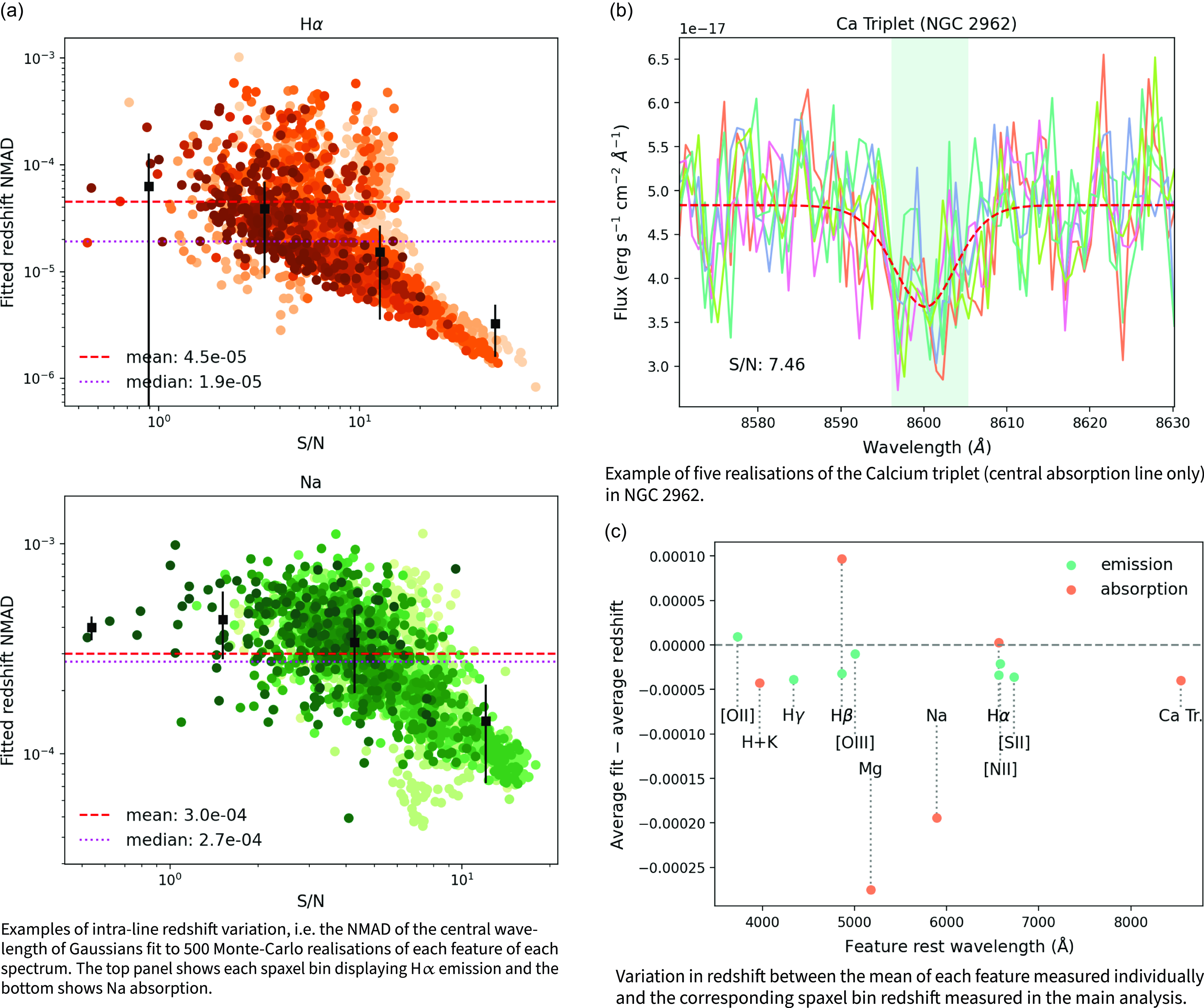
(a) shows the variation in fits to the central wavelength of the individual features of H $\alpha$
emission and Na absorption. Each spectrum was realised 500 times, varying the pixel flux by a Gaussian with a width of the measured noise, then Gaussians were fit to those features. Each point in these figures is the variation in those centres, converted to redshift, and each galaxy is a different colour. The mean and median of these are shown in the red dashed and magenta dotted lines, respectively, and overplotted in black are the binned data. (b) shows five of the 500 realisations in solid lines of a particular spaxel bin of the galaxy NGC 2962. The red dashed line shows the normalised sum of all 500 fitted Gaussians. The green window is a five Å rest wavelength window about the canonical redshift used to estimate the S/N of the feature. (c) shows the variation caused by measuring single features when compared to the redshift measured from Marz, with emission (green) and absorption (orange) differentiated (H
$\alpha$
emission and Na absorption. Each spectrum was realised 500 times, varying the pixel flux by a Gaussian with a width of the measured noise, then Gaussians were fit to those features. Each point in these figures is the variation in those centres, converted to redshift, and each galaxy is a different colour. The mean and median of these are shown in the red dashed and magenta dotted lines, respectively, and overplotted in black are the binned data. (b) shows five of the 500 realisations in solid lines of a particular spaxel bin of the galaxy NGC 2962. The red dashed line shows the normalised sum of all 500 fitted Gaussians. The green window is a five Å rest wavelength window about the canonical redshift used to estimate the S/N of the feature. (c) shows the variation caused by measuring single features when compared to the redshift measured from Marz, with emission (green) and absorption (orange) differentiated (H $\alpha$
and H
$\alpha$
and H $\beta$
occur in both, sometimes within different regions of the same galaxy). The dotted lines simply aid in identifying each feature.
$\beta$
occur in both, sometimes within different regions of the same galaxy). The dotted lines simply aid in identifying each feature.
5.2 Redshift uncertainty
Since in most cases we have many spectra for the same galaxy and many features in those spectra, we can estimate the variation in redshift caused by noise as a measure of precision. We can do this in two ways: the first is to measure the variation of wavelength determination of individual features, and the second is to measure the variation between multiple features. Both can be achieved by measuring the redshift of many realisations of each spectrum with the flux of each pixel shifted by a Gaussian whose standard deviation is the measured noise of that pixel. The method that utilises multiple features is more appropriate for characterising redshift uncertainty as measuring redshift from a single feature is very rarely trustworthy (unless it is particularly high S/N and/or has resolved substructure), but here we already have a tight prior on the redshift, and we are mainly interested in its variation rather than its value. Instead of running each realisation of each spectrum through Marz, we opt to fit the features using Gaussians and convert the central wavelength to a redshift. This method is highly scaleable (no user interface and low computation time); however, it may still be interesting to compare the robust correlation method to the simplified Gaussian fitting. Note that we cannot simply use the width of the correlation peak given by Marz to estimate redshift uncertainty as it is at least an order of magnitude larger than our actual precision.
Each spectrum was assigned tags for which features were present with enough S/N to be able to at least somewhat reliably fit Gaussians (both absorption and emission). 500 realisations of each spectrum were generated, and a $\pm$
30 Å rest wavelength window containing each feature was extracted, using the outer edges to estimate and subtract the continuum. A Gaussian was then fit to each feature; the fit was rejected if it was more than 10 Å from the known wavelength, if it was unreasonably wide or low amplitude, (accounting for the fact absorption lines are generally wider and shallower than emission), and if the amplitude was positive (negative) for emission (absorption) lines, all of which indicate a failure to capture the feature of interest. A five Å rest wavelength window around the known wavelength was also used to estimate the S/N of each feature from the original spectrum.
$\pm$
30 Å rest wavelength window containing each feature was extracted, using the outer edges to estimate and subtract the continuum. A Gaussian was then fit to each feature; the fit was rejected if it was more than 10 Å from the known wavelength, if it was unreasonably wide or low amplitude, (accounting for the fact absorption lines are generally wider and shallower than emission), and if the amplitude was positive (negative) for emission (absorption) lines, all of which indicate a failure to capture the feature of interest. A five Å rest wavelength window around the known wavelength was also used to estimate the S/N of each feature from the original spectrum.
The features we applied this process to were: H $\alpha$
, H
$\alpha$
, H $\beta$
(both of which can be in both emission and absorption), H
$\beta$
(both of which can be in both emission and absorption), H $\gamma$
, Na, Mg, along with the second line of each of O[II], O[III], N[II], S[II], and the CaII H+K and infrared triplet absorption features. The NMAD of the fitted wavelengths measures how much the redshift can shift within the bounds of the measured noise, and when plotted against S/N shows a strong trend of increasing precision with increasing S/N. The mean of all of the fitted wavelengths when compared with the known redshift measures how much the redshift can shift according to which features are present or most prominent. This in particular should be a more accurate reflection of the total redshift precision. Given the type of galaxy/features and S/N, an estimate of redshift precision can be made. Ideally this would be done on an individual redshift basis, but we save a more thorough treatment for future work.
$\gamma$
, Na, Mg, along with the second line of each of O[II], O[III], N[II], S[II], and the CaII H+K and infrared triplet absorption features. The NMAD of the fitted wavelengths measures how much the redshift can shift within the bounds of the measured noise, and when plotted against S/N shows a strong trend of increasing precision with increasing S/N. The mean of all of the fitted wavelengths when compared with the known redshift measures how much the redshift can shift according to which features are present or most prominent. This in particular should be a more accurate reflection of the total redshift precision. Given the type of galaxy/features and S/N, an estimate of redshift precision can be made. Ideally this would be done on an individual redshift basis, but we save a more thorough treatment for future work.
Fig. 15 shows examples of the methods described above and Table 2 shows the numerical results. Fig. 15a shows the ‘intra-line’ variation of the H $\alpha$
emission and Na absorption features against their S/N estimates, while Fig. 15b shows an example of the average Gaussian fit to the 500 realisations of the calcium triplet of one spaxel bin of NGC 2962 (host of SN 1995D). The S/N is just an estimate because the five Å window used to estimate it is too wide for some emission lines and too narrow for some absorption lines. Occasionally, the noise is overestimated and/or the flux is underestimated (e.g. the cases of reduction failures), which is why we see S/N < 1 but solid feature detection. Finally, emission lines are naturally higher S/N than absorption lines, so 1:1 comparisons between the two can be misleading. In general though, especially at high S/N, which was the aim of this program, we see excellent precision. However, some features do not show a trend with S/N (such as the hydrogen absorption lines and calcium H + K), which may be due to their presence at lower S/N in general and/or a Gaussian fit being less appropriate.
$\alpha$
emission and Na absorption features against their S/N estimates, while Fig. 15b shows an example of the average Gaussian fit to the 500 realisations of the calcium triplet of one spaxel bin of NGC 2962 (host of SN 1995D). The S/N is just an estimate because the five Å window used to estimate it is too wide for some emission lines and too narrow for some absorption lines. Occasionally, the noise is overestimated and/or the flux is underestimated (e.g. the cases of reduction failures), which is why we see S/N < 1 but solid feature detection. Finally, emission lines are naturally higher S/N than absorption lines, so 1:1 comparisons between the two can be misleading. In general though, especially at high S/N, which was the aim of this program, we see excellent precision. However, some features do not show a trend with S/N (such as the hydrogen absorption lines and calcium H + K), which may be due to their presence at lower S/N in general and/or a Gaussian fit being less appropriate.
Summary of spectral feature fitting precision, converted to redshift. Rest wavelengths are taken from Marz and converted from vacuum to air, except for the calcium triplet which comes from the Vienna Atomic Line Database. For doublets and triplets, we consider only the second line.
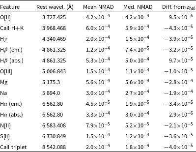
Fig. 15c shows the offset between the redshift via a single feature and the Marz redshift. These measurements are found from taking the mean of the mean offsets for each feature and spaxel bin compared to their Marz measured redshift. The emission lines are generally in much closer agreement with the final redshift measurement; the reason Mg and Na in particular are not in agreement is due to their complex line profiles. Since these lines are (sometimes significantly) asymmetrical and deeper in the blue end than the red, the fitted wavelength is biased blue. While the Gaussian fit for these lines is biased, the intra-line variation should be robust to the exact location of the centre of the Gaussian approximation.
In conclusion of this investigation, the high S/N emission line galaxy redshifts are precise to better than several ${10^{-5}}$
, the high S/N absorption galaxies and low S/N emission line galaxies are precise to better than approximately 1
${10^{-5}}$
, the high S/N absorption galaxies and low S/N emission line galaxies are precise to better than approximately 1 ${\times 10^{-4}}$
, and the low S/N absorption galaxies are not generally present.
${\times 10^{-4}}$
, and the low S/N absorption galaxies are not generally present.
5.3 Cosmological results
To quantify the effect of our redshift updates on cosmology, we use the entire SH0ES/Pantheon+ cosmology sampleFootnote
i
(photometry and Cepheid calibration) and the Pippin
Footnote
j
end-to-end SN cosmology analysis pipeline (Hinton & Brout Reference Hinton and Brout2020). This method allows us to calculate SH0ES/Pantheon+ distance moduli using the redshifts of this work as well as take advantage of the statistical+systematic covariance matrix C for both the original and updated redshift sample. For each of the redshifts we remeasure, we transform to the CMB frame then recalculate peculiar velocity using pvhub
Footnote
k
to correct to the cosmological frame ( ${z_{\text{HD}}^{\mathrm{}}}$
). The average change in peculiar velocity was zero, but individually they varied by up to
${z_{\text{HD}}^{\mathrm{}}}$
). The average change in peculiar velocity was zero, but individually they varied by up to $\pm80$
km s
$\pm80$
km s $^{-1}$
(
$^{-1}$
( $\pm 2.7{\times 10^{-4}}$
in redshift);Footnote
l
in comparison, around 15% of the redshift shifts are larger than these maximal peculiar velocity shifts (see the right panel of Fig. 13).
$\pm 2.7{\times 10^{-4}}$
in redshift);Footnote
l
in comparison, around 15% of the redshift shifts are larger than these maximal peculiar velocity shifts (see the right panel of Fig. 13).
With our new set of cosmological redshifts ${z_{\text{HD}}^{\mathrm{}}}$
, Pantheon+ light curves and SH0ES calibrations, we perform a simultaneous fit for
${z_{\text{HD}}^{\mathrm{}}}$
, Pantheon+ light curves and SH0ES calibrations, we perform a simultaneous fit for $H_0$
and
$H_0$
and $\Omega_{\text{m}}$
in a flat
$\Omega_{\text{m}}$
in a flat $\Lambda$
CDM Universe (i.e.
$\Lambda$
CDM Universe (i.e. $\Omega_\Lambda=1-\Omega_{\text{m}}$
,
$\Omega_\Lambda=1-\Omega_{\text{m}}$
, $w=-1$
) by minimising distance modulus residuals defined by
$w=-1$
) by minimising distance modulus residuals defined by
 \begin{equation} \Delta \mu_i = \mu_{\text{obs},i} - \mu_{\text{model}}(z_{\text{HD},i},H_0,\Omega_{\text{m}}),\end{equation}
where i spans the set of Pantheon+ light curves. Briefly, Pippin makes use of SNANA (Kessler et al. Reference Kessler2009) to take input photometry, redshifts, etc. and calculate $\mu_{\text{obs},i}$
from a modified Tripp equation of the form
$\mu_{\text{obs},i}$
from a modified Tripp equation of the form
 \begin{equation} \mu_{\text{obs}} = m+\alpha x_1 - \beta c - M - \delta_{\text{bias}} + \delta_{\text{host}},\end{equation}
where light curve peak magnitude m (equivalent to B-band magnitude), stretch $x_1$
and colour c are fit with an updated SALT2 model (Guy et al. Reference Guy2010; Brout et al. Reference Brout2022b),
$x_1$
and colour c are fit with an updated SALT2 model (Guy et al. Reference Guy2010; Brout et al. Reference Brout2022b), $\alpha$
and
$\alpha$
and $\beta$
are nuisance parameters, M is the absolute magnitude of SNe Ia,
$\beta$
are nuisance parameters, M is the absolute magnitude of SNe Ia, $\delta_{\text{bias}}$
are observational bias corrections estimated from simulations, and
$\delta_{\text{bias}}$
are observational bias corrections estimated from simulations, and $\delta_{\text{host}}$
accounts for the residual correlation between SN Ia brightness and host mass. For more details, see Hinton & Brout (Reference Hinton and Brout2020), Brout et al. (2022a). The theoretical distance moduli
$\delta_{\text{host}}$
accounts for the residual correlation between SN Ia brightness and host mass. For more details, see Hinton & Brout (Reference Hinton and Brout2020), Brout et al. (2022a). The theoretical distance moduli $\mu_{\text{model}}$
are calculated directly from the cosmological model as
$\mu_{\text{model}}$
are calculated directly from the cosmological model as
 \begin{equation} \mu_{\text{model}}(z) = 5\log_{10}(D_{\text{L}}(z))+25,\end{equation}
with luminosity distance $D_{\text{L}}$
in Mpc, calculated from
$D_{\text{L}}$
in Mpc, calculated from
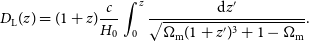 \begin{equation} D_{\text{L}}(z) = (1+z)\frac{c}{H_0} \int_{0}^{z} \frac{\text{d}z^\prime}{\sqrt{\Omega_{\text{m}}(1+z^\prime)^3 + 1-\Omega_{\text{m}}}}.\end{equation}
For Cepheid calibrated galaxies, $\mu_{\text{model}}(z_i)$
is replaced with
$\mu_{\text{model}}(z_i)$
is replaced with $\mu_i^{\text{Cepheid}}$
. With the vector of residuals
$\mu_i^{\text{Cepheid}}$
. With the vector of residuals $\Delta\boldsymbol{\mu}$
, the best-fit cosmology comes from minimising the function
$\Delta\boldsymbol{\mu}$
, the best-fit cosmology comes from minimising the function
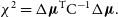 \begin{equation} \chi^2 = \Delta \boldsymbol{\mu}^ {\text{T}} \text{C}^{-1} \Delta {\boldsymbol{\mu}}.\end{equation}
Of the 185 SN host galaxies we measured, 146 galaxies and 215 light curvesFootnote m passed the quality cuts to be used in the fit.
This determination of $H_0$
is equivalent to fitting the intercept of the linear distance-redshift relation, as done by SH0ES (Riess et al. Reference Riess2022). The intercept,
$H_0$
is equivalent to fitting the intercept of the linear distance-redshift relation, as done by SH0ES (Riess et al. Reference Riess2022). The intercept, $a_\mathrm{B}$
, is constrained by galaxies whose motion is dominated by expansion. It is standard practice to use the (third-order) cosmographic expansion of recession velocity, which is almost exact in the ‘Hubble Flow’ redshift range used for fitting
$a_\mathrm{B}$
, is constrained by galaxies whose motion is dominated by expansion. It is standard practice to use the (third-order) cosmographic expansion of recession velocity, which is almost exact in the ‘Hubble Flow’ redshift range used for fitting $H_0$
(
$H_0$
( $0.0233 \lt {z_{\text{HD}}^{\mathrm{}}} \lt 0.15$
):
$0.0233 \lt {z_{\text{HD}}^{\mathrm{}}} \lt 0.15$
):
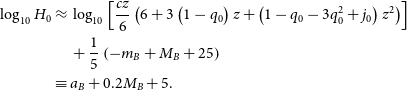 \begin{align} \log_{10}H_0 \approx & \; \log_{10}\left[\frac{cz}{6}\left(6+3\left(1-q_0\right)z+\left(1-q_0-3q_0^2+j_0\right)z^2\right)\right] \nonumber \\ & \; +\frac{1}{5}\left(-m_B + M_B + 25\right)\nonumber \\ \equiv & \; a_B+0.2M_B+5.\end{align}
The expansion includes the cosmic deceleration parameter ( $q_0=-0.55$
) and jerk (
$q_0=-0.55$
) and jerk ( $j_0=1.0$
), whose values are chosen to match the standard
$j_0=1.0$
), whose values are chosen to match the standard $\Lambda$
CDM model with
$\Lambda$
CDM model with $(\Omega_{\text{m}},\Omega_{\Lambda,w}) = (0.3,0.7,-1)$
. As such, this fitting method has weak cosmological model dependence. Since the dependence is weak, this method can still be used to constrain cosmologies whose parameters are somewhat near the input parameters.
$(\Omega_{\text{m}},\Omega_{\Lambda,w}) = (0.3,0.7,-1)$
. As such, this fitting method has weak cosmological model dependence. Since the dependence is weak, this method can still be used to constrain cosmologies whose parameters are somewhat near the input parameters.
Left: full Hubble diagram showing the SNe used to constrain and the residuals of the best-fit flat $\Lambda$
CDM cosmology
$\Lambda$
CDM cosmology $(H_0, \Omega_{\text{m}}) = (72.6$
km s
$(H_0, \Omega_{\text{m}}) = (72.6$
km s $^{-1}$
Mpc
$^{-1}$
Mpc $^{-1}$ $, 0.328)$
. Right: change in individual
$, 0.328)$
. Right: change in individual $\mu$
, normalised to the best-fit cosmology of the updated redshift sample. Galaxies with
$\mu$
, normalised to the best-fit cosmology of the updated redshift sample. Galaxies with ${z_{\text{HD}}^{\mathrm{\ }}} \lt 0.0233$
are greyed out because they are not used to determine
${z_{\text{HD}}^{\mathrm{\ }}} \lt 0.0233$
are greyed out because they are not used to determine $H_0$
. The change from original (green) to updated (orange) in magnitude space is often too small to see. The error bars, shown only for the updated sample, come from the covariance matrix statistical and systematic uncertainty added in quadrature (for display purposes only). The weighted average shift in
$H_0$
. The change from original (green) to updated (orange) in magnitude space is often too small to see. The error bars, shown only for the updated sample, come from the covariance matrix statistical and systematic uncertainty added in quadrature (for display purposes only). The weighted average shift in $\mu$
of
$\mu$
of $-5{\times 10^{-4}}$
mag from the original sample corresponds to a shift in
$-5{\times 10^{-4}}$
mag from the original sample corresponds to a shift in $H_0$
of
$H_0$
of $+0.1$
km s
$+0.1$
km s $^{-1}$
Mpc
$^{-1}$
Mpc $^{-1}$
.
$^{-1}$
.
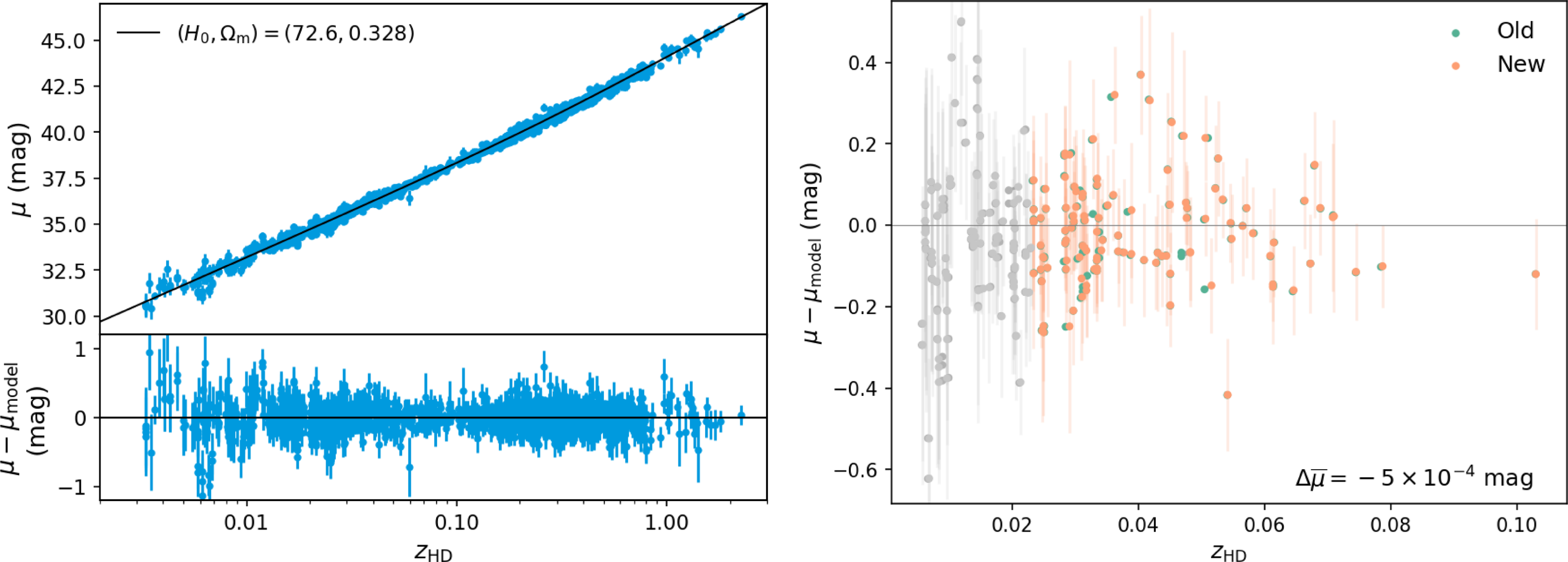
An input cosmology also enters into our analysis in the simulations used to perform bias corrections, and this dependence is also weak (Camilleri et al. Reference Camilleri2024). The results of our fit are shown in Fig. 16; the Hubble diagram of the sample including our redshift updates has a best-fit cosmology $(H_0, \Omega_{\text{m}}) = (72.6\pm1.2$
km s
$(H_0, \Omega_{\text{m}}) = (72.6\pm1.2$
km s $^{-1}$
Mpc
$^{-1}$
Mpc $^{-1}$
,
$^{-1}$
, $0.328^{+0.018}_{-0.017})$
, and the weighted average difference in distance moduli from the sample with original redshifts is only
$0.328^{+0.018}_{-0.017})$
, and the weighted average difference in distance moduli from the sample with original redshifts is only $-5{\times 10^{-4}}$
mag, equivalent to a difference in
$-5{\times 10^{-4}}$
mag, equivalent to a difference in $H_0$
of
$H_0$
of $0.1$
km s
$0.1$
km s $^{-1}$
Mpc
$^{-1}$
Mpc $^{-1}$
. The error bars we show are the statistical and systematic uncertainties from the covariance matrix, added in quadrature. It should be noted that even when including the 250 km s
$^{-1}$
. The error bars we show are the statistical and systematic uncertainties from the covariance matrix, added in quadrature. It should be noted that even when including the 250 km s $^{-1}$
uncertainty in peculiar velocities (
$^{-1}$
uncertainty in peculiar velocities ( $\sim8{\times 10^{-4}}$
when converted to redshift), redshift uncertainties propagated through to
$\sim8{\times 10^{-4}}$
when converted to redshift), redshift uncertainties propagated through to $H_0$
are completely subdominant to these distance modulus uncertainties. Within the SH0ES/Pantheon+ Hubble flow range, our 146 redshifts represent approximately a quarter of all SNe that have high-quality light curves.
$H_0$
are completely subdominant to these distance modulus uncertainties. Within the SH0ES/Pantheon+ Hubble flow range, our 146 redshifts represent approximately a quarter of all SNe that have high-quality light curves.
Since we are using magnitudes calibrated with the SH0ES distance ladder, we see similar central values of $H_0$
to SH0ES (
$H_0$
to SH0ES ( $73.04\pm1.04$
km s
$73.04\pm1.04$
km s $^{-1}$
Mpc
$^{-1}$
Mpc $^{-1}$
; Riess et al. Reference Riess2022), but only the shift in
$^{-1}$
; Riess et al. Reference Riess2022), but only the shift in $H_0$
from our redshift changes is important here. Thus, the key takeaway from this work is that the shift in
$H_0$
from our redshift changes is important here. Thus, the key takeaway from this work is that the shift in $H_0$
from the original sample purely due to our redshift updates is only
$H_0$
from the original sample purely due to our redshift updates is only $0.1$
km s
$0.1$
km s $^{-1}$
Mpc
$^{-1}$
Mpc $^{-1}$
, which is negligible compared to the 1.2 km s
$^{-1}$
, which is negligible compared to the 1.2 km s $^{-1}$
Mpc
$^{-1}$
Mpc $^{-1}$
uncertainty of each fit. We can also calculate an individual
$^{-1}$
uncertainty of each fit. We can also calculate an individual $H_0$
directly for each of the host galaxies in our sample from Equation (4) with
$H_0$
directly for each of the host galaxies in our sample from Equation (4) with $\Omega_{\text{m}}=0.3$
, replacing the left-hand-side with
$\Omega_{\text{m}}=0.3$
, replacing the left-hand-side with $D_{\text{L}}(\mu_{\text{obs}})$
, and taking the weighted average before and after the redshift updates gives the same result of
$D_{\text{L}}(\mu_{\text{obs}})$
, and taking the weighted average before and after the redshift updates gives the same result of $0.1$
km s
$0.1$
km s $^{-1}$
Mpc
$^{-1}$
Mpc $^{-1}$
. This is not unexpected from the magnitude of the changes to redshift, and a similar result was found in Carr et al. (Reference Carr2022) although opposite in sign. The average redshift correction was an order of magnitude larger in Carr et al. (Reference Carr2022) in the same direction, so the result of this work is likely just a statistical fluctuation. Our result reinforces the general conclusion that while redshift errors have the potential to bias
$^{-1}$
. This is not unexpected from the magnitude of the changes to redshift, and a similar result was found in Carr et al. (Reference Carr2022) although opposite in sign. The average redshift correction was an order of magnitude larger in Carr et al. (Reference Carr2022) in the same direction, so the result of this work is likely just a statistical fluctuation. Our result reinforces the general conclusion that while redshift errors have the potential to bias $H_0$
, the reality is that any realistic redshift errors are too small to affect
$H_0$
, the reality is that any realistic redshift errors are too small to affect $H_0$
.
$H_0$
.
6. Conclusion
We have shown with our new observations that indeed there exist errors in the previous measurements of the redshifts of nearby SN Ia host galaxies. The differences had a negligible systematic offset, which was reflected in the negligible change to $H_0$
.
$H_0$
.
We thoroughly examined the instrumental accuracy with three probes in Section 4. We tracked the wavelength solution corrections due to temperature fluctuations as measured from our frequent calibrations between science observations. We also examined the wavelength solution accuracy across the whole aperture by checking the skyline emission spectrum on a per-night and per-run basis. Similarly, we also compared spatially binned redshifts with accurately known radial velocity standard stars. In no case did we find a need for corrections to our redshifts, and therefore we have shown our redshifts to be accurate to within a couple of ${10^{-5}}$
.
${10^{-5}}$
.
However, there are several extensions to our analysis that can be made to further investigate the sources of the redshift errors in the interest of mitigating them in the future. Firstly, while we saw good agreement between averaging the redshift over all spaxels and just the core sections, it would be beneficial to investigate why we still see scatter at the level of about 3 ${\times 10^{-5}}$
. In addition, the rest of the cases of very large redshift discrepancies (rather than just the two largest) can be examined by comparing with original spectra where possible. Finally, for many galaxies (about half of our sample), we will be able to measure the redshift of the region around where the SN actually occurred within the galaxy. This would be a useful crosscheck with previous redshifts, as there may be a correlation between those redshifts and the historical redshifts of Pantheon+ in the cases where a long-slit spectrograph was aligned with the SN but not the core, or a fibre-pointing inaccuracy. It is also useful for observing the local SN environment and examining SN Ia brightness and host/environment correlations, as there is a wealth of information beyond the redshifts to explore. As an example of how integral-field observations can be used, the high-spatial-resolution spectrograph MUSE has been used as part of the All-weather MUSE Integral-field Nearby Galaxies (AMUSING; Galbany et al. Reference Galbany2016) survey to characterise the environments of Type Ia (Holoien et al. Reference Holoien2023) and core-collapse SNe (Pessi et al. Reference Pessi2023).
${\times 10^{-5}}$
. In addition, the rest of the cases of very large redshift discrepancies (rather than just the two largest) can be examined by comparing with original spectra where possible. Finally, for many galaxies (about half of our sample), we will be able to measure the redshift of the region around where the SN actually occurred within the galaxy. This would be a useful crosscheck with previous redshifts, as there may be a correlation between those redshifts and the historical redshifts of Pantheon+ in the cases where a long-slit spectrograph was aligned with the SN but not the core, or a fibre-pointing inaccuracy. It is also useful for observing the local SN environment and examining SN Ia brightness and host/environment correlations, as there is a wealth of information beyond the redshifts to explore. As an example of how integral-field observations can be used, the high-spatial-resolution spectrograph MUSE has been used as part of the All-weather MUSE Integral-field Nearby Galaxies (AMUSING; Galbany et al. Reference Galbany2016) survey to characterise the environments of Type Ia (Holoien et al. Reference Holoien2023) and core-collapse SNe (Pessi et al. Reference Pessi2023).
In this work, we study the overall accuracy and precision of our redshifts, but we have not characterised individual precisions for our redshifts, which would be a function of the spectrum S/N and number of spaxel bins for a galaxy. Instead we give a general uncertainty class depending on the S/N and galaxy type/prominent features. This can be taken further to provide individual estimates, which would mostly be useful to differentiate the lower quality observations, as our high S/N data are extremely accurate and precise for an optical spectrograph without simultaneous wavelength solution measurement (from, e.g., frequency combs). For the purposes of measuring $H_0$
, our redshift data can essentially be taken as constants, at least until the peculiar velocity and distance modulus uncertainty floor is drastically improved. This has already been done historically for convenience, but for our sample this is a valid assumption; however, it does not necessarily hold for other purposes which may be even more sensitive to redshift errors.
$H_0$
, our redshift data can essentially be taken as constants, at least until the peculiar velocity and distance modulus uncertainty floor is drastically improved. This has already been done historically for convenience, but for our sample this is a valid assumption; however, it does not necessarily hold for other purposes which may be even more sensitive to redshift errors.
While we have confirmed that remeasuring accurate redshifts does not have an effect on $H_0$
, we stress it is still important to use accurate and precise redshifts for cosmology, especially as we gather more and more spectroscopic data. Importantly, at least at high-redshift, we will have to start using photometric redshifts and SN classifications, as spectroscopic follow-up becomes unfeasible from the expected volume of data from future surveys, such as the Legacy Survey of Space and Time (Ivezić et al. Reference Ivezicć2019), which will add new forms of systematic error to investigate.
$H_0$
, we stress it is still important to use accurate and precise redshifts for cosmology, especially as we gather more and more spectroscopic data. Importantly, at least at high-redshift, we will have to start using photometric redshifts and SN classifications, as spectroscopic follow-up becomes unfeasible from the expected volume of data from future surveys, such as the Legacy Survey of Space and Time (Ivezić et al. Reference Ivezicć2019), which will add new forms of systematic error to investigate.
Supplementary material
The supplementary material for this article can be found at https://doi.org/10.1017/pasa.2024.74
Acknowledgement
The authors thank S. Sweet for useful discussions and advice on observation optimisation, and S. Hinton for creating the Marz redshifting program and assisting in modifying it for our purposes. The authors thank C. Howlett, J. Calcino, and K. Said for assistance in carrying out observations and M. Craigie for assistance in target selection.
TMD is the recipient of an Australian Research Council Australian Laureate Fellowship (project number FL180100168) funded by the Australian Government. DS is supported by DOE grants DE-SC0010007, DE-SC0021962 and the David and Lucile Packard Foundation. DS is supported in part by the National Aeronautics and Space Administration (NASA) under Contract No. NNG17PX03C issued through the Roman Science Investigation Teams Programme.
This work is based on data acquired at Siding Spring Observatory with the ANU 2.3m Telescope via programs 1200040, 2200080, 3200100, and 4200059. We acknowledge the traditional custodians of the land on which the telescope stands, the Gamilaraay people, and pay our respects to elders past and present. This research was also supported by resources provided by the University of Chicago Research Computing Center and used services provided by the Astro Data Lab at the US National Science Foundation’s National Optical-Infrared Astronomy Research Laboratory. NOIRLab is operated by the Association of Universities for Research in Astronomy (AURA), Inc. under a cooperative agreement with the National Science Foundation. This work has also made use of the VALD database, operated at Uppsala University, the Institute of Astronomy RAS in Moscow, and the University of Vienna.
Data availability statement
Data obtained as part of this work are available on Zenodo (https://doi.org/10.5281/zenodo.10884817).


 Open access