

1. INTRODUCTION
Variegated Glacier is a surge-type glacier in Alaska, whose 20th-century surge history is well documented (Lawson, Reference Lawson1997; Eisen and others, Reference Eisen, Harrison and Raymond2001; Harrison and others, Reference Harrison2008). Numerous field campaigns between 1973 and 1984 yielded an extensive dataset covering the 1982/83 surge and second half of the antecedent quiescent phase. The position of many surface markers was determined twice a year prior to and 8 times during the surge, which resulted in a long record of surface elevation and velocity measurements (Bindschadler and others, Reference Bindschadler, Harrison, Raymond and Crosson1977b; Raymond and Harrison, Reference Raymond and Harrison1988). Data on bed elevation and surface width was gathered during the first two field campaigns (Bindschadler and others, Reference Bindschadler, Harrison, Raymond and Crosson1977b), and surface mass-balance measurements were obtained between 1973 and 1979 (Bindschadler, Reference Bindschadler1982). Additionally, data on basal water pressure, water transit time and outlet discharge was collected before, during and after the surge.
The large dataset has proven to be extremely valuable for research into surge behaviour. Bindschadler and others (Reference Bindschadler, Harrison, Raymond and Crosson1977b) analysed the data available in 1995 and proved that around the surge cycle midpoint ice motion occurred predominantly by internal deformation. They also demonstrated that the actual ice flux was far smaller than the balance flux, elucidating the progressive changes in glacier geometry during quiescence. Kamb and others (Reference Kamb1985) studied the data on water pressure, transit time and outflow. They inferred that the high velocities during surge were caused by high basal water pressures and reasoned that a switchover in basal drainage system from an efficient channel system during quiescence to an inefficient linked cavity system during surge facilitated these high pressures. A reverse switch would mark surge termination.
Humphrey and others (Reference Humphrey, Raymond and Harrison1986) examined water transit times and terminus outflow during the occurrence of mini-surges in the years just prior to surge initiation in 1982. Based on a consideration of continuity and flow through Röthlisberger tunnels, they reasoned that the upper part of the glacier was underlain by a drainage system with a large total cross-sectional area but restricted flow passageways, i.e. an inefficient, distributed drainage system, whereas the lower part was underlain by an efficient channel system. Raymond and others (Reference Raymond, Johannesson, Pfeffer and Sharp1987) studied the propagation of the 1982/83 surge front and found evidence for water retention behind this front. They rejected the idea that this water ponding was caused by blockage of basal water flow through the front due to high normal ice stresses acting as a pressure dam, but did not find compelling evidence for one of the alternative explanations.
Raymond (Reference Raymond1987) analysed all data and tried to find general answers to questions about surge mechanism. They noted that the two surge pulses composing the 1982/83 surge had a distinct seasonal timing, viz., they both initiated in winter and terminated in early summer, indicating a connection between surge initiation/termination and seasonally varying surface water abundance. They furthermore concluded that stress redistribution caused rapid spreading of the initial, small surge nucleus across a region of active ice, after which a steadily growing topographic peak formed, which eventually propagated downstream following the theory of kinematic waves.
Raymond and Harrison (Reference Raymond and Harrison1988) examined the gradual evolution of glacier geometry and velocity during quiescence. They demonstrated that especially in the reservoir area and after 1978 changes in surface velocity were larger than could be expected from changes in driving stress and ice thickness. Hence, either ice softened considerably or sliding became increasingly important. Assuming the latter, they inferred the pattern and evolution of sliding and concluded that this pattern/evolution requires the sliding velocity to be directly proportional to basal shear stress and inversely proportional to the local effective pressure. They additionally showed that not a single combination of steady-state water drainage through Röthlisberger tunnels and existing theories relating sliding velocity to basal shear stress and effective pressure, could adequately simulate the inferred pattern and evolution. As the switch theory proposed by Kamb and others (Reference Kamb1985) includes drainage through an efficient channel system during quiescence, the study by Raymond and Harrison (Reference Raymond and Harrison1988) casts doubt about the switch theory's correctness.
Humphrey and Raymond (Reference Humphrey and Raymond1994) analysed the discharge in the outlet streams during surge and inferred that the basal hydraulic system consisted of an inefficient, distributed system in the surge zone while an efficient channel system underlay the stagnant zone. Moreover, they reasoned that not basal water pressure but instead volume of water stored in the distributed system was the prime hydraulic control on ice motion during the 1982/83 surge. Eisen and others (Reference Eisen, Harrison and Raymond2001) studied the 20th-century surge history of Variegated Glacier and found a correlation between cumulative mass balance and quiescent phase duration, indicating that surge recurrence interval is climatically controlled. Harrison and others (Reference Harrison2008) corroborated this connection. Harrison and Post (Reference Harrison and Post2003) found evidence for subglacial till under Variegated Glacier and speculated that till is a prerequisite for surge behaviour. The observations covered only a fraction of the glacier, hence it might be possible to reconcile these observations with the linked-cavity model of surge motion proposed by Kamb and others (Reference Kamb1985).
Eisen and others (Reference Eisen2005) looked at the distinct seasonal timing of surge initiation and termination. They hypothesised a mechanism for surge initiation similar to the one proposed by Kamb and others (Reference Kamb1985). They supplemented their idea with a concrete switch criterion depending on basal shear stress and surface meltwater input. Jay-Allemand and others (Reference Jay-Allemand, Gillet-Chaulet, Gagliardini and Nodet2011) reconstructed the evolution of basal conditions prior to and during the 1982/83 surge using an inverse method. Their research showed that surge initiation and propagation coincided with an abrupt dramatic decrease in basal friction. By incorporating an effective pressure dependent friction law, they linked small basal friction to basal water pressure approaching overburden pressure. The sudden change in water pressure accompanying surge initiation and propagation was then ascribed to a switch from an efficient channel system during quiescence to an inefficient linked cavity system during surge, corroborating the theory proposed by Kamb and others (Reference Kamb1985).
All these studies shed light on the mechanism behind Variegated Glacier's surge behaviour. Nevertheless, there are missing pieces and there is lack of consensus. To resolve the surge mechanism of this particular glacier and compare it with the unifying theory proposed by Sevestre and Benn (Reference Sevestre and Benn2015); find the factors that distinguish this glacier from surrounding normal glaciers; and eventually, for example, judge the surging potential of polar ice masses, further research is necessary. However, there are no ongoing field campaigns resulting in new in-situ measurements and, moreover, analyses of satellite data does not yield new insights (Harrison and others, Reference Harrison2008). A significant step could be made, though, by using the extensive dataset obtained through the field campaigns between 1973 and 1984 in simulating Variegated Glacier's surge cycle with a two-component basal drainage system model coupled with an ice flow model, as suggested by Jay-Allemand and others (Reference Jay-Allemand, Gillet-Chaulet, Gagliardini and Nodet2011). This new step is facilitated by recent work on a criterion for the dynamic switching between channel and cavity system (Schoof, Reference Schoof2010) and recent work on a model that accounts for partially filled drainage systems (underpressure) and ice-bed separation (overpressure) (Hewitt and others, Reference Hewitt, Schoof and Werder2012; Schoof and others, Reference Schoof, Hewitt and Werder2012).
The original dataset is predominantly of flow line nature, hence it seems naturally to apply a flow line model. However, simply applying the somewhat fragmentary centre line data inevitably entails problems. Bindschadler (Reference Bindschadler1982, unpublished) and Raymond and Harrison (Reference Raymond and Harrison1988), for example, ran into discrepancies between the ice flux determined from data on surface mass balance and ice thickness change and the ice flux deduced from velocity measurements. They concluded that such deviations are inherent in applying centre line data to a specific three-dimensional system. Likewise, Jay-Allemand and others (Reference Jay-Allemand, Gillet-Chaulet, Gagliardini and Nodet2011) assigned discrepancies between model results and observations to 3-D effects.
The present paper aims at extrapolating surface elevation profiles into the upper and lower parts of the glacier and at adapting the centre line data to cover 3-D effects. For that purpose, a comprehensive survey of reported quantitative and qualitative observations is conducted. Readjustments to the centre line data should account for differences between width-averaged and centre line surface mass balance and ice thickness change, for tributary inflow and for changes in surface width during a surge cycle. The 3-D effects are considered to be represented properly when physical constraints regarding ice flux, specific mass balance and net volume change are met. Subsequent application of the original as well as the revised dataset in a simple 1-D flow line model illustrates the effect of the performed data optimisation.
2. ORIGINAL DATASET
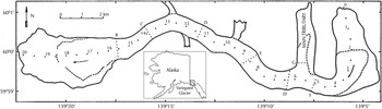
Between 1973 and 1984, every spring or early summer numerous surface markers were spread along the central flow line between KM 3 and KM 18, over the upper part of the accumulation zone and across seven transverse sections, see Figure 1. Where possible, the position of the markers was measured twice a year prior to and 8 times during the 1982/83 surge. Average summer speed was determined by subtracting marker positions at the start and end of the melting season. Average winter speed was obtained similarly, but only for those markers that survived winter. This yielded a long, but somewhat fragmentary record of surface elevation and velocity measurements (Bindschadler and others, Reference Bindschadler, Harrison, Raymond and Crosson1977b; Raymond and Harrison, Reference Raymond and Harrison1988).
Map of Variegated Glacier, Alaska, showing distance from the glacier head (km) along the central flow line. The dashed lines represent the boundaries of the zone affected by the 1982/83 surge, and the dotted lines show the locations of the seven transverse sections B through G. The arrows indicate the general flow direction. Modified from: Kamb and others (Reference Kamb1985).
Seismic reflection during the first two field campaigns yielded bed elevation measurements along the central flow line and across several transverse sections. Later, these observations were supplemented with radio echo-sounding and bore-hole depth measurements (Raymond and Harrison, Reference Raymond and Harrison1988). Surface width was measured at the transverse sections during the first two field campaigns and a longitudinal profile was constructed by interpolating/extrapolating the gathered data based on US Geological Survey map sheets (Raymond and Harrison, Reference Raymond and Harrison1988).
Surface mass balance was measured along the centre line, over the main tributary, and across transverse sections B through F between 1973 and 1979. The coverage varied from year to year but is considered good in the ablation zone, where surface lowering due to ablation was measured using wires frozen into boreholes. Coverage is less satisfactory in the accumulation zone. Up till 1976, surface mass balance was measured in a pit at section F, and, less accurately, by probing and looking at crevasse walls at a few other points. As of 1976, magnet markers were used to obtain reliable measurements of net accumulation above KM 3.
Before, during and after the 1982/83 surge, boreholes were drilled to the glacier bed. Water levels in these boreholes were recorded, and additionally water tracer dye was injected to obtain values for water transit time between these boreholes and the glacier terminus. Also, discharge in the outlet streams was measured. All collected data were submitted to the World Data Centre – Glaciology and is currently stored at the Scott Polar Research Institute of the University of Cambridge (Bindschadler and others, Reference Bindschadler, Harrison and Raymond1974, Reference Bindschadler, Harrison and Raymond1975, Reference Bindschadler, Harrison and Raymond1976, Reference Bindschadler, Harrison and Raymond1977a; Raymond and others, Reference Raymond, Harrison, MacQueen and Gitomer1978, Reference Raymond1980, Reference Raymond, Harrison, MacQueen and Senear1981, Reference Raymond, Harrison, MacQueen and Senear1988).
3. SURFACE ELEVATION PROFILES
The longitudinal surface elevation profiles constructed out of measurements are incomplete, see the solid lines in Figure 2. Data are missing especially during and after the surge. Eisen and others (Reference Eisen2005) and Jay-Allemand and others (Reference Jay-Allemand, Gillet-Chaulet, Gagliardini and Nodet2011) presented July 1983 surface elevation profiles extending from head to snout, however their extrapolated parts differ considerably. This paper aims at constructing well-founded complete profiles for September 1981 and July 1983, i.e. at the end of the quiescent respectively surge phase. Extrapolations are based on documented qualitative observations as well as suitable measurements at other moments in time. A heavily crevassed surface made measurements below KM 18 impossible and no effort is made to extend the profiles beyond this point.
Surface elevation profiles along the central flow line. Solid lines show the measured parts in the key months September 1981 (red) and July 1983 (blue), i.e. at the end of the quiescent respectively surge phase; and in June 1973 (green) and September 1984 (yellow), i.e. at the time of the first respectively last field campaign. Most profiles are incomplete in the upper and/or lower part of the glacier. The dotted lines depict the extrapolated parts of the September 1981 and July 1983 profiles. The grey line represents the bed elevation.

The original September 1981 surface elevation profile is almost complete. Observations are lacking solely below KM 17. It is noted that thinning in the receiving area during quiescence increases with distance from the glacier head (Raymond, Reference Raymond1987). As a conservative guess, thinning below KM 17 is assumed equal to the measured thinning at KM 17. The missing part of the September 1981 profile is constructed accordingly, i.e. by subtracting the thinning at KM 17 between June 1973 and September 1981 from the June 1973 profile below KM 17, see the dotted part of the red line in Figure 2.
The July 1983 surface elevation profile needs to be extrapolated above KM 4.75 and below KM 17.75. It is reminded that during quiescence changes in glacier geometry are gradual. Hence, thickness changes between July 1983 and September 1984 are limited and September 1984 surface elevations thus form a good approximation for missing July 1983 elevations, see the part of the dotted blue line on top of the solid yellow line in Figure 2. Moreover, aerial photographs revealed that above KM 2 the glacier was only mildly affected by the 1982/83 surge, which was assigned to the presence of an ice fall between KM 2 and 2.7 (Raymond and Harrison, Reference Raymond and Harrison1988). Accordingly, above KM 2 the July 1983 profile is assumed identical to the June 1973 and September 1981 profiles, see the part of the dotted blue line on top of the solid red line in Figure 2. What remains is the part between KM 2 and 3.5. It is assumed that after a full surge cycle glaciers return to their initial geometry, i.e. the quiescent phase and surge phase are characterised by equal but reverse changes in geometry. When, in addition, it is assumed that the thickening/thinning is evenly distributed over the corresponding phase, the thinning during the 1982/83 surge is twice the thickening during the second half of the antecedent quiescent phase. The remaining part of the July 1983 profile is constructed accordingly, i.e. by multiplying the thickening between June 1973 and September 1981 by 2 and subtracting it from the September 1981 profile. The extrapolated profiles are given in the Supplementary material.
4. 3-D EFFECTS
Applying a sophisticated flow line model to Variegated Glacier requires a dataset that accounts for lateral effects. The raw centre line data does not meet this requirement, hence it has to be adapted. The revised dataset should cover differences between width-averaged and centre line ice thickness change and surface mass balance as well as inflow from tributaries. Moreover, it should capture the significant changes in glacier surface width during a surge cycle due to the combination of substantial ice thickness changes and gently sloping sidewalls.
4.1. Observations
A first set of adaptations is based on a combination of quantitative and qualitative observations.
4.1.1. Width-averaged ice thickness change
Centre line ice thickness change during the 1982/83 surge is determined by subtracting the extrapolated July 1983 surface elevation profile from the September 1981 profile. Similarly, centre line ice thickness change during the second half of the antecedent quiescent phase is obtained from the September 1981 and June 1973 profiles. This method does not provide values for the thickness change in the terminal zone as the surface profiles are not extended beyond KM 18. Fortunately, thickness change in this zone can be estimated from Supplementary remarks. Aerial photographs revealed that the 1982/83 surge front got as far as KM 18.5, see Figure 1. By lack of more data, thickening between KM 18 and 18.5 is assigned the value at KM 18. Concerning the second half of the quiescent phase, Raymond and Harrison (Reference Raymond and Harrison1988) reported a thinning of more than 50 m in the zone downstream of KM 18, hence thickness change below KM 18 is assigned this value.
Two parameters are introduced to account for differences between width-averaged thickness changes,
 $\overline {\Delta H} $
and centre line thickness changes, ΔH, during the 1982/83 surge respectively the antecedent quiescent phase:
$\overline {\Delta H} $
and centre line thickness changes, ΔH, during the 1982/83 surge respectively the antecedent quiescent phase:
 $$\alpha _{surge}(x) = \displaystyle{{{\overline {\Delta H}} _{surge}(x)} \over {\Delta H_{surge}(x)}},\quad \alpha _{quies}(x) = \displaystyle{{{\overline {\Delta H}} _{quies}(x)} \over {\Delta H_{quies}(x)}},$$
where x is distance from the glacier head along the flow line. Appropriate values for these ratios can be deduced from reported qualitative observations. Figure 1 shows that between KM 2–4 and KM 16–18.5 only part of the cross section was affected by the 1982/83 surge. Between KM 2 and 4, the affected area was laterally bounded by a ridge, and, below KM 16, the abrupt glacier widening caused the surge front to spread out into a bulb-like lobe that did not reach the side margins, see Figure 3. In these regions, width-averaged thickness change deviates considerably from centre line thickness change. To account for this discrepancy, locally their ratio is assigned a value smaller than one, i.e. α surge < 1 between KM 2–4 and KM 16–18.5. As a first guess, it is assumed that the ratio between width-averaged and centre line thickness change equals the ratio between affected and total surface width. The latter ratio can be estimated from Figure 1. α surge is then schematised as decreasing linearly from 1 to 0.5 between KM 2 and 3 and increasing inversely between KM 3–4. Similarly, α surge is schematised as decreasing linearly from 1 to 0.8 between KM 16–17.25 and from 0.8 to 0 between KM 17.25 and 18.5.
The background shows a composite of aerial photographs taken just after the 1983 surge termination (Lawson, Reference Lawson1997). Part of the upper basin is overlain by a brighter map (Google Earth, 2011) to illustrate the presence of a ridge (indicated by the red arrow) as well as high, steep ice-clad valley walls.

Regarding quiescence, there is no information on lateral variation in thickness change. For the region between KM 2 and 4, it is surmised α quies equals α surge . Below KM 16, centre line thinning more or less equaled local ablation, indicating that ice flow in this part of the glacier was limited. Hence, downstream of KM 16 lateral variation in thinning is expected to be modest, and, accordingly, the ratio between width-averaged and centre line thickness change during quiescence α quies is set to 1.
4.1.2. Width-averaged surface mass balance
A linear least square fitting technique is applied to the average surface mass-balance profile over the period 1973–79. The result is a function that captures the height-mass-balance feedback:
 $$\dot b(x) = 0.0062(h(x) - 1098),$$
where
 $\dot b$
is centre line surface mass balance (m a−1) and h is surface elevation (m). This equation reveals an equilibrium line altitude of 1098 m a.s.l. To account for differences between width-averaged surface mass balance,
$\dot b$
is centre line surface mass balance (m a−1) and h is surface elevation (m). This equation reveals an equilibrium line altitude of 1098 m a.s.l. To account for differences between width-averaged surface mass balance,
 $\overline {\dot b} $
, and its centre line value, a third parameter, β, is introduced:
$\overline {\dot b} $
, and its centre line value, a third parameter, β, is introduced:
 $$\overline {\dot b} (x) = \dot b(x) + \beta (x).$$
Figure 4 pictures surface mass-balance contour lines based on balance year 1972/73. The contours clearly show ablation diminishing towards the side margins in the lower half of the glacier, probably representing snow accumulation from avalanches down steep valley walls. This is further demonstrated in Figure 5, which depicts surface mass-balance measurements across three transverse sections in the ablation zone. At transverse section D, net ablation decreases solely towards the southern margin. Moreover, locally the centre line value more or less resembles the constructed width-averaged value. At section C, the difference between width-averaged and centre line ablation is on average 1.2 m a−1, whereas the difference is once again limited at section B. The contours in Figure 4 do not show a clear pattern in the accumulation zone. Accordingly, the difference β is schematised as increasing linearly from 0.0 to 1.2 m a−1 between KM 12.5–14 and decreasing inversely between KM 14–15.5, and 0.0 elsewhere.
Surface mass-balance contours (solid lines – m w.e. a−1) based on balance year 1972/73. The dotted lines represent the locations of transverse measurement sections B through F. Up till 1976, almost no surface mass-balance measurements were made in the upper accumulation zone, hence the contour lines do not extend into this part of the glacier. Modified from: Bindschadler and others (Reference Bindschadler, Harrison and Raymond1974).

Surface mass balance across transverse sections D, C and B for balance years 1972/73 (red), 1973/74 (blue) and 1974/75 (grey). Nine markers were spread across each transverse section: one at the centre line, four to the North (1Dn, 2Dn, etc.), and four to the South (1Ds, 2Ds, etc.). The crosses, solid dots and open circles represent respectively centre line measurements, off-centre measurements and interpolated/extrapolated values used to determine width-averaged surface mass balance. Six measurements across a section is considered the minimum for a reasonably reliable width-averaged value (horizontal dotted lines).

4.1.3. Tributary inflow
Ice flow from tributaries into the glacier trunk can be considerable and should therefore be accounted for in a model. No quantitative observations are available on tributaries other than the main one, i.e. the one entering the trunk between KM 5.5 and 6.5, hence for the moment only this tributary is considered. The main tributary thinned during the 1982/83 surge and thickened during the antecedent quiescent phase (Raymond and Harrison, Reference Raymond and Harrison1988), so its flux into the glacier trunk varied over time. Ideally, this tributary would be modelled by a separate flow line that merges with the glacier trunk near KM 6, however this is prohibited by the highly limited amount of data regarding the tributary. So, instead, the tributary is considered as a whole with distinct fluxes into the trunk during quiescence and surge.
The tributary's balance flux is given by
 $Q_{main} = \overline {\dot b} _{main}{\kern 1pt} A_{main}$
, where
$Q_{main} = \overline {\dot b} _{main}{\kern 1pt} A_{main}$
, where
 $\overline {\dot b} _{main}$
is the main tributary's spatial average surface mass balance and A
main
is its surface area. However, the tributary is not in balance, viz., it thinned during the 1982/83 surge and thickened during the antecedent quiescent phase (Raymond and Harrison, Reference Raymond and Harrison1988). Hence, during surge (quiescence) the inflow from this tributary is larger (smaller) than its balance flux. The volume fluxes can be calculated by subtracting the spatial average thickness change,
$\overline {\dot b} _{main}$
is the main tributary's spatial average surface mass balance and A
main
is its surface area. However, the tributary is not in balance, viz., it thinned during the 1982/83 surge and thickened during the antecedent quiescent phase (Raymond and Harrison, Reference Raymond and Harrison1988). Hence, during surge (quiescence) the inflow from this tributary is larger (smaller) than its balance flux. The volume fluxes can be calculated by subtracting the spatial average thickness change,
 $\overline {\Delta H} _{main}$
, from the ice layer added at the surface during this period of time,
$\overline {\Delta H} _{main}$
, from the ice layer added at the surface during this period of time,
 $\overline {\dot b} _{main}{\kern 1pt} T$
, which results in
$\overline {\dot b} _{main}{\kern 1pt} T$
, which results in
 $$Q_{main} = \displaystyle{{{\overline {\dot b}} _{main}{\kern 1pt} T - {\overline {\Delta H}} _{main}} \over T}A_{main}.$$
Measurements of
 $\overline {\dot b} _{main}$
and A
main
are at hand. Surface marker positions, and thus ice thickness changes, were measured solely near the confluence and then only occasionally. No quantitative information is available on the thinning during the 1982/83 surge. It seems reasonable to equate the thinning near the confluence to the local thinning in the glacier trunk, which was ~75 m. Figure 1 reveals that only one third of the tributary was affected by the surge. When it is assumed that this fraction serves as a good estimate for the ratio between area-averaged thinning and thinning near the connection point, the volume flux during the 1982/83 surge was ~87.9e6 m3 a−1.
$\overline {\dot b} _{main}$
and A
main
are at hand. Surface marker positions, and thus ice thickness changes, were measured solely near the confluence and then only occasionally. No quantitative information is available on the thinning during the 1982/83 surge. It seems reasonable to equate the thinning near the confluence to the local thinning in the glacier trunk, which was ~75 m. Figure 1 reveals that only one third of the tributary was affected by the surge. When it is assumed that this fraction serves as a good estimate for the ratio between area-averaged thinning and thinning near the connection point, the volume flux during the 1982/83 surge was ~87.9e6 m3 a−1.
Raymond and Harrison (Reference Raymond and Harrison1988) stated that the tributary thickened by ~40 m near the confluence between 1973 and 1978, whereas its surface did not rise during the remainder of the quiescent phase. Nothing is reported on the part of the tributary that experienced thickening. When it is assumed that the same area that was affected by the surge thickened during the preceding quiescent phase, the volume flux during quiescence was ~9.7e6 m3 a−1.
4.1.4. Varying surface width
The cross-sectional geometry was found to be more or less parabolic (Bindschadler and others, Reference Bindschadler, Harrison, Raymond and Crosson1977b). Hence, glacier surface width varies over a surge cycle, following the local ice thickness, according to
 $$W_s(x) = 2{\kern 1pt} \sqrt {\displaystyle{{H(x)} \over {a(x)}}}, $$
where W s is surface width, H is centre line ice thickness and a is the leading parabola coefficient, which indicates the broadness/narrowness of the transverse profile. An appropriate longitudinal profile for this coefficient can be obtained from the 1973 surface width, surface elevation and bed elevation profiles. Subsequently applying the September 1981 and July 1983 surface elevation profiles reveals changes in surface width of up to 50% during a surge cycle. This demonstrates that accounting for evolving width is important.
4.2. Constraints
The dataset adaptations suggested above are primarily based on quantitative and qualitative observations. They comprise incorporation of three parameters to account for differences between width-averaged and centre line ice thickness change and surface mass balance; inclusion of a two-valued inflow from the main tributary; and application of ice thickness dependent glacier surface width instead of fixed surface width. Physical constraints on ice volume flux, specific mass balance and net volume change present additional alterations.
4.2.1. Ice flux
Ice volume flux can be determined from data on surface mass balance and ice thickness change as well as from velocity measurements. The resulting longitudinal profiles should be equal, nonetheless Bindschadler (Reference Bindschadler1982, unpublished) and Raymond and Harrison (Reference Raymond and Harrison1988) detected excessive discrepancies between both profiles. Constructing the two ice flux profiles and subsequently resolving the encountered discrepancies will introduce new dataset adaptations. Data on ice velocity is fragmentary, especially during surge, as crevasses prevented measuring the position of all markers. During quiescence, ice velocity changes gradual with time so that missing data can be approximated by linear interpolation. On the contrary, the dynamic behaviour during surge does not allow for linear interpolation. Hence, only the flux profiles during the quiescent phase preceding the 1982/83 surge are constructed and examined.
Ice flux in the glacier trunk can be determined from data on surface mass balance and ice thickness change similar to the inflow from the main tributary (Eqn (4)):
 $$Q(x) = \int_0^x \displaystyle{{\overline {\dot b} (x){\kern 1pt} T_{quies} - {\overline {\Delta H}} _{quies}(x)} \over {T_{quies}}}{\kern 1pt} W_s(x){\kern 1pt} {\rm d}x,$$
where T quies is the considered time period, i.e. June 1973 till September 1981. When the inflow from the main tributary is schematised as a point source at KM 6.5, the flux downstream of this point becomes
 $$\eqalign{Q(x \vert x \ge 6.5) = & \int_0^x \displaystyle{{\overline {\dot b} (x){\kern 1pt} T_{quies} - {\overline {\Delta H}} _{quies}(x)} \over {T_{quies}}}W_s(x){\kern 1pt} {\rm d}x \cr & + Q_{main,quies}.} $$
Alternatively, the ice volume flux can be deduced from velocity measurements according to
 $$Q_{vel}(x) = \overline u (x){\kern 1pt} A_{\,flow}(x),$$
where A
flow
is the cross-sectional area through which ice flows, and
 $\overline u $
is the corresponding area-averaged horizontal ice velocity. The area of parabolic cross-sectional profiles is given by
$\overline u $
is the corresponding area-averaged horizontal ice velocity. The area of parabolic cross-sectional profiles is given by
 $A(x) = 2/3{\kern 1pt} W_s(x)H(x)$
. Between KM 2 and KM 4, the already mentioned ridge presumably prevents ice from flowing through the whole valley, see Figure 3, hence locally the active cross-sectional area A
flow
is smaller than the total cross-sectional area A. A parameter, γ, is introduced to account for this difference:
$A(x) = 2/3{\kern 1pt} W_s(x)H(x)$
. Between KM 2 and KM 4, the already mentioned ridge presumably prevents ice from flowing through the whole valley, see Figure 3, hence locally the active cross-sectional area A
flow
is smaller than the total cross-sectional area A. A parameter, γ, is introduced to account for this difference:
 $$A_{\,flow}(x) = \displaystyle{2 \over 3}{\kern 1pt} \gamma (x){\kern 1pt} W_s(x)H(x).$$
Identical to the ratio between width-averaged and centre line thickness change α, the ratio between active and total cross-sectional area γ is deemed equal to the ratio of glacier surface width affected by the 1982/83 surge to total surface width. γ is thus schematised as decreasing linearly from 1 to 0.5 between KM 2 and 3 and increasing inversely between KM 3 and 4, and 1 elsewhere. The cross-section averaged ice velocity can be estimated using (derivation given in Appendix A)
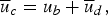
 $$\overline u (x) = \left( {\displaystyle{3 \over 5} + \displaystyle{3 \over {20}}\displaystyle{{u_b} \over {u_s}}(x)} \right)u_s(x),$$
where u s is the measured centre line surface velocity and u b /u s is the ratio between sliding and surface velocity. Jay-Allemand and others (Reference Jay-Allemand, Gillet-Chaulet, Gagliardini and Nodet2011) inferred longitudinal profiles of this ratio using an inverse method. The in this paper applied profile resembles the average of their ‘S 1976’ and ‘W 76-77’ patterns.
4.2.2. Specific mass balance
A constraint is imposed on adjustments to the fitted surface mass-balance function: a positive specific mass balance is con sidered unrealistic. Specific mass balance, B, of the glacier system is defined as
 $$B = \displaystyle{{\int_0^L \overline {\dot b} (x){\kern 1pt} W_s(x){\kern 1pt} {\rm d}x + {\overline {\dot b}} _{main}{\kern 1pt} A_{main} + Q_{add}} \over {\int_0^L W_s(x){\kern 1pt} {\rm d}x}},$$
where L is glacier length and Q add represents additional mass inflow from, for example, another tributary. Variegated Glacier has a length of ~20 km, but no data are collected below KM 18. However, to obtain a realistic value for the specific mass balance, the integral in (11) has to be taken over the full glacier length. Accordingly, surface mass balance and width are extrapolated into the terminal zone downstream of KM 18 by assigning their values at KM 18.
4.2.3. Net volume change
It is believed that surge cycles are characterised by an ongoing internal redistribution of mass without net mass loss/gain. Apart from ongoing retreat/advance as a response to climate change, surge-type glaciers are expected to reach their original geometry, and thus volume, after a full surge cycle. Raymond (Reference Raymond1987) concluded that Variegated Glacier's volume had increased during its 1982/83 surge, probably due to the generation of void space as a result of the convex upward ice motion at the surge front. Hence, ice volume is expected to have shrunk in the antecedent quiescent phase. This volume loss may not be captured by the dataset as it may have occurred during the unobserved first half of the quiescent phase. Therefore, a somewhat milder restriction is imposed on the net volume change during the second half of the quiescent phase:
 $$\Delta V_{quies,net} = \Delta V_{quies} - B{\kern 1pt} T_{quies} \le 0,$$
in which the net volume change is given as a volume change per unit surface area, i.e. in m. The volume change between 1973 and 1981 is calculated using
 $$\eqalign{\Delta V_{quies} = & \displaystyle{{\int_0^L {\overline {\Delta H}} _{quies}(x){\kern 1pt} W_s(x){\kern 1pt} {\rm d}x} \over {\int_0^L W_s(x){\rm d}x}} \cr & + \displaystyle{{{\overline {\Delta H}} _{main,quies}{\kern 1pt} A_{main}} \over {\int_0^L W_s(x){\rm d}x}}.} $$
For completeness, net volume gain during the 1982/83 surge is determined and evaluated.
4.3. Dataset adaptations
Table 1 and Figure 6 present specific mass balance and volume change values as well as quiescent phase ice flux profiles for four different dataset versions, namely the original centre line dataset and three cumulatively adapted datasets. The discussed physical constraints are met when in Table 1 specific mass balance B and net volume change during quiescence ΔV quies,net are nonpositive and net volume change during surge ΔV surge,net is positive, and when in Figure 6 the flux profile determined from data on surface mass balance and ice thickness change (red line) resembles the profile deduced from velocity measurements (green line).
Ice volume flux along the central flow line averaged over the period 1973–1981. The green line shows the flux deduced from velocity measurements that should be resembled by the flux determined from data on surface mass balance and ice thickness change (red lines). The dotted, dash-dot, dashed and solid red lines depict the ice volume flux corresponding to respectively dataset versions 1, 2, 3 and 4, see Table 1.

Results for the original dataset and three cumulatively adapted versions

The third column presents specific mass balance, and net volume change during quiescence (surge) is given in column four (five). The last line shows the imposed constraints.
For the original dataset (version 1), Table 1 indicates a tremendous volume gain during quiescence. Additionally, Figure 6 reveals that the ice volume flux computed from data on surface mass balance and ice thickness change (dotted red line) is far too small and even negative over the vast majority of the glacier. Applying the adaptations determined from qualitative and quantitative observations on 3-D effects (version 2) improves the results considerably: it reduces (enlarges) the net volume gain during quiescence (surge) and diminishes the discrepancy between the two ice flux profiles. In more detail, the dash-dot red line lies above the dotted red line and captures the bulge near KM 6.5, i.e. the inflow from the main tributary. The size of the bulges in the dash-dot red line and green line is comparable, which indicates that the deduced inflow is realistic.
Despite the improvement, the flux profile computed from data on surface mass balance and ice thickness change still does not resemble the profile deduced from velocity measurements. Figure 6 shows that below KM 4 the dash-dot red line lies far below the green line while its slope is broadly correct. The required uniform vertical shift below KM 4 points to a larger width-averaged surface mass balance and/or a smaller width-averaged thickening above KM 4, see Eqn (6). Aerial photographs of Variegated Glacier reveal considerable valley walls between KM 2 and 4, see Figure 3. Avalanches down these high, steep ice-clad walls may accumulate significant amounts of snow at their bottom, causing the width-averaged surface mass balance to locally exceed the centre line value, i.e β > 0. The ice-clad valley walls cover an area of ~2, 000 · 1, 000 = 2, 000, 000 m2. Assuming that snow accumulation on the valley walls between KM 2 and 4 equals the centre line accumulation at KM 3, avalanches down these high, steep walls may dump up to
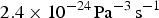
 $2,000,000 \!\cdot\! 2.6 = 5.2 \!\cdot\! 10^6{\kern 1pt} {\rm m}^3{\rm a}^{ - 1}$
of ice on the glacier surface. This corresponds to an additional width-averaged accumulation of β = 1.4 m a−1 between KM 2 and 4. Whereas there is no mention of avalanches in reports, the presence of high, steep ice-clad walls makes them plausible.
$2,000,000 \!\cdot\! 2.6 = 5.2 \!\cdot\! 10^6{\kern 1pt} {\rm m}^3{\rm a}^{ - 1}$
of ice on the glacier surface. This corresponds to an additional width-averaged accumulation of β = 1.4 m a−1 between KM 2 and 4. Whereas there is no mention of avalanches in reports, the presence of high, steep ice-clad walls makes them plausible.
This larger width-averaged surface mass balance between KM 2 and 4 fails to provide the total required vertical shift below KM 4. A smaller width-averaged thickening between KM 2 and 4 may resolve the remaining discrepancy. By lack of data on the lateral variation in thickness change during quiescence, the ratio between width-averaged and centre line thickness change was set equal to the corresponding ratio during surge. The latter ratio, in turn, was set equal to the ratio of glacier surface width affected by the 1982/83 surge to total surface width. However, width-averaged thickness change is probably smaller as this first guess assumes that the surge motion caused a depression with vertical walls, whereas a bowl-shaped depression might be more realistic. Multiplying the earlier suggested values for α quies = α surge by 0.25 between KM 2 and 4 realises the remaining part of the required vertical shift below KM 4.
Version 3 of the dataset incorporates the suggested larger width-averaged surface mass balance and smaller width-averaged thickness change between KM 2 and 4. The resulting dataset meets the constraints regarding specific mass balance and net volume change during quiescence and surge, see Table 1. However, a look at Figure 6 reveals that the corresponding flux profile (dashed red line) does not completely follow the flux profile deduced from velocity measurements. Firstly, it does not capture the substantial bulge ~KM 10. This bulge is attributed to inflow from three smaller tributaries between KM 8 and KM 10, see Figure 1. A combined inflow from these tributaries of
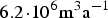 $6.2 \!\cdot\! 10^6{\kern 1pt} {\rm m}^3{\rm a}^{ - 1}$
yields a correct bulge size. This inflow is approximately two-thirds of the inflow from the main tributary, which seems reasonable considering the associated catchment areas in Figure 1. The three smaller tributaries are not affected by the 1982/83 surge, hence the deduced volume flux is applicable to both phases of the surge cycle.
$6.2 \!\cdot\! 10^6{\kern 1pt} {\rm m}^3{\rm a}^{ - 1}$
yields a correct bulge size. This inflow is approximately two-thirds of the inflow from the main tributary, which seems reasonable considering the associated catchment areas in Figure 1. The three smaller tributaries are not affected by the 1982/83 surge, hence the deduced volume flux is applicable to both phases of the surge cycle.
Secondly, below KM 13 the slope of the dashed red line is too gentle and even becomes positive. We note that ablation causes a negative flux gradient, whereas thinning causes a positive gradient, see Eqn (7). Steady lower width-averaged surface mass balance and/or steady smaller width-averaged thinning below KM 13 could thus diminish the discrepancy in flux gradient. There are no observation that support such corrections. However, we should at least resolve the nonphysical positive flux gradient near the glacier tongue. The lateral variation in thinning below KM 16 was assumed to be modest, so that, as a first guess, the local ratio between width-averaged and centre line thickness change α quies was set to 1. Requiring a nonpositive flux gradient, i.e. width-averaged thinning is not allowed to exceed width-averaged ablation, results in slightly lower values (~0.9) for α quies below KM 13.5.
The fourth and final version of the dataset integrates these two corrections. It meets the constraints regarding specific mass balance and net volume change during quiescence, and, moreover, the corresponding flux profile satisfactorily resembles the profile deduced from velocity measurements. The revised dataset pinpoints a volume gain during the 1982/83 surge of 12.7 m per unit surface area, which corresponds to a glacier volume increase of ~9.4%. Raymond (Reference Raymond1987) detected a volume increase reaching 10% in the lower part of the surge zone. At the end of the 1982/83 surge, the surge zone covered a major part of the glacier, hence both figures seem compatible. The deduced inflow from tributaries is depicted in Table 2, whereas the other revisions are given in the Supplementary material.
Inflow from the main tributary and the so-called second tributary, which in fact combines three smaller tributaries
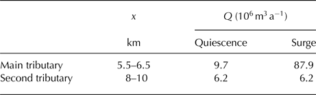
The second column represents the confluence's distance from the glacier head along the flow line and the third and fourth column give the corresponding inflow during quiescence respectively surge. The main tributary is affected by the 1982/83 surge, hence its flux into the glacier trunk varies over a surge cycle.
5. APPLICATION
Both the original and revised dataset are used as input into a 1-D flow line model similar to the one first applied in Oerlemans (Reference Oerlemans1986). The model solves the continuity equation for incompressible ice integrated over the glacier cross section:
 $$\displaystyle{{\partial A} \over {\partial t}} = - \displaystyle{\partial \over {\partial x}}(\overline u A_{\,flow}) + \overline {\dot b} W_s.$$
For a parabolic cross-sectional profile with A flow = γA, this equation can be written as (derivation given in Appendix B)
 $$\displaystyle{{\partial H} \over {\partial t}} = - \displaystyle{2 \over {3W_s}}\displaystyle{\partial \over {\partial x}}(\gamma {\kern 1pt} \overline u {\kern 1pt} W_sH) + \overline {\dot b}. $$
Following the Shallow Ice Approximation (SIA) for internal deformation and a Weertman-type law for sliding, depth-averaged centre line velocity
 $\overline u _c$
is determined locally from the driving stress τ
d
according to (Budd and others, Reference Budd, Keage and Blundy1979)
$\overline u _c$
is determined locally from the driving stress τ
d
according to (Budd and others, Reference Budd, Keage and Blundy1979)
 $$\overline u _c = f_dH\tau _d^n + f_s\displaystyle{{\tau _d^n} \over H},$$
where f d and f s are flow parameters for respectively internal deformation and sliding, and n is the exponent in Glen's flow law. Assuming a value of 3/4 for the ratio between width-averaged and centre line velocity and taking Glen's flow law exponent equal to 3, results in the following expression for the cross section averaged horizontal velocity:
 $$\overline u = \displaystyle{3 \over 4}\left( {\,f_dH\tau _d^3 + f_s\displaystyle{{\tau _d^3} \over H}} \right).$$
The driving stress is defined as
 $$\tau _d = - s\rho gH\displaystyle{{\partial h} \over {\partial x}},$$
where s is the shape factor, ρ is the ice density and g is the gravitational acceleration. Substituting these equations in (15) results in
 $$\displaystyle{{\partial H} \over {\partial t}} = \displaystyle{1 \over {2W_s}}\displaystyle{\partial \over {\partial x}}\left( {\gamma D\displaystyle{{\partial h} \over {\partial x}}} \right) + \overline {\dot b}, $$
with the diffusivity D given by
 $$D = (\,f_dH^2 + f_s)(s\rho g)^3H^3\left( {\displaystyle{{\partial h} \over {\partial x}}} \right)^2W_s.$$
Eqn (18) is solved explicitly, i.e. W
s
, D and
 $\overline {\dot b} $
are calculated from the results of the previous time step. To allow the glacier to grow beyond KM 18, the measured bed topography is extrapolated by means of an exponential fit to the profile above KM 18. In the run with the original dataset, the fitted linear surface mass-balance profile (Eqn (2)) and the measured 1973 surface width profile are applied. In the run with the revised dataset, on the other hand, surface width is modelled using Eqn (5). Moreover, this run incorporates all suggested dataset revisions to account for 3-D effects. Inflow from the main and three smaller tributaries is included in the imposed surface mass balance and schematised as evenly distributed mass sources between respectively KM 5.5–6.5 and KM 8–10. In both runs, the shape factor profile deduced by Bindschadler (Reference Bindschadler1982) is implemented. Finally, Table 3 depicts the applied parameter values.
$\overline {\dot b} $
are calculated from the results of the previous time step. To allow the glacier to grow beyond KM 18, the measured bed topography is extrapolated by means of an exponential fit to the profile above KM 18. In the run with the original dataset, the fitted linear surface mass-balance profile (Eqn (2)) and the measured 1973 surface width profile are applied. In the run with the revised dataset, on the other hand, surface width is modelled using Eqn (5). Moreover, this run incorporates all suggested dataset revisions to account for 3-D effects. Inflow from the main and three smaller tributaries is included in the imposed surface mass balance and schematised as evenly distributed mass sources between respectively KM 5.5–6.5 and KM 8–10. In both runs, the shape factor profile deduced by Bindschadler (Reference Bindschadler1982) is implemented. Finally, Table 3 depicts the applied parameter values.
Parameter values used in the SIA simulations

The deformation flow parameter f
d
can be expressed in Glen's flow law parameters A and n according to f
d
= 2A/(n + 2). The rheology parameter A is set to
 $2.4 \times 10^{ - 24}{\kern 1pt} {\rm P}{\rm a}^{ - 3}\,{\rm s}^{ - 1}$
, appropriate for ice at 0° (Cuffey and Paterson, Reference Cuffey and Paterson2010). This value is compatible with values considered appropriate for similar glaciers (Oerlemans, Reference Oerlemans1997a, Reference Oerlemansb; Zuo and Oerlemans, Reference Zuo and Oerlemans1997; Giesen and Oerlemans, Reference Giesen and Oerlemans2010). f
s
is chosen such that the ratio between sliding and surface velocity in the original dataset run more or less resembles the ‘W 76-77’ pattern deduced by Jay-Allemand and others (Reference Jay-Allemand, Gillet-Chaulet, Gagliardini and Nodet2011).
$2.4 \times 10^{ - 24}{\kern 1pt} {\rm P}{\rm a}^{ - 3}\,{\rm s}^{ - 1}$
, appropriate for ice at 0° (Cuffey and Paterson, Reference Cuffey and Paterson2010). This value is compatible with values considered appropriate for similar glaciers (Oerlemans, Reference Oerlemans1997a, Reference Oerlemansb; Zuo and Oerlemans, Reference Zuo and Oerlemans1997; Giesen and Oerlemans, Reference Giesen and Oerlemans2010). f
s
is chosen such that the ratio between sliding and surface velocity in the original dataset run more or less resembles the ‘W 76-77’ pattern deduced by Jay-Allemand and others (Reference Jay-Allemand, Gillet-Chaulet, Gagliardini and Nodet2011).
Simple steady-state runs are performed. In brief, incorporating the proposed dataset revisions enlarges the (steady-state) ice flux, which is expressed in a larger ice thickness, velocity and glacier length. Figure 7 shows the resulting surface elevation profiles together with the measured September 1981 (end quiescent phase) and July 1983 (end surge phase) profiles. The original dataset run culminates in a steady-state volume 38% larger than the 1973 volume, which coincides with the number found by Bindschadler (Reference Bindschadler1982) based on the same dataset. The revised dataset returns a 147% larger volume and thus even more convincingly shows that Variegated Glacier's steady-state volume is considerably larger than its volume as a surge-type glacier. In steady state, Variegated Glacier would be thicker and longer than ever observed. To grow towards and eventually approach equilibrium, the reservoir area would first need to build-up, after which a slow dynamic response would cause the receiving area to thicken and the glacier to lengthen. The progressive changes in glacier geometry during quiescence imitate the required build-up of the reservoir area. This implies that the glacier evolution during quiescence is basically the growth back towards steady state after the glacier was brought out of balance by a surge. Steady state is, however, never reached because long before a new surge is triggered. Surface mass balance is the driving force of the build-up of the reservoir area, hence a change in external forcing may effect the duration of the quiescent phase.
Steady-state surface elevation profiles from SIA model runs with the original (yellow) and revised (green) dataset. For comparison, the extrapolated profiles at the end of the quiescent phase (red), respectively, surge phase (blue) are depicted.

6. DISCUSSION AND CONCLUSIONS
Applying a flow line model to Variegated Glacier to conduct research into its surge mechanism requires a dataset that accounts for lateral effects. In this paper, the original centre line data covering the 1982/83 surge and antecedent quiescent phase was extrapolated into the upper and lower parts of the glacier as well as revised to incorporate various 3-D effects. Unfortunately, remarks on lateral variation in surface mass balance and thickness change were scarce, while information on the inflow from tributaries other than the main one was absent. Nevertheless, the sparse observations provided a first set of dataset modifications. Physical constraints on ice volume flux, specific mass balance and net volume change presented additional adaptations. Although the latter revisions are not backed-up by observations, they do have clear, plausible physical explanations. For example, the bulge near KM 10 in the flux profile deduced from velocity measurements clearly indicated a local, substantial ice source. A look at Variegated Glacier's map revealed the presence of three smaller tributaries and despite the fact that no report mentioned them, the bulge was assigned to inflow from these tributaries.
Meeting the imposed constraint regarding ice volume flux during quiescence required a larger width-averaged surface mass balance and/or smaller width-averaged thickening above KM 4. It was speculated that avalanches down high, steep ice-clad valley walls between KM 2 and 4 accumulate significant amounts of snow at the bottom of these walls, augmenting the local width-averaged surface mass balance. Likewise, it was surmised that the depression associated with surge motion is bowl-shaped rather than rectangular-shaped, reducing the width-averaged thickness change above KM 4. A very rough, upper estimate of snow accumulation due to avalanches between KM 2 and 4 was made and the remaining part of the required vertical shift in ice volume flux profile was realised by decreasing the ratio between width-averaged and centre line thickening above KM 4, viz., a more narrow bowl-shaped depression. This method resulted in a local minimum of 0.13 for the ratio between width-averaged and centre line thickening. This value is considered (too) low, nonetheless raising it is inconvenient as that would necessitate an even higher value for the snow accumulation due to avalanches. It should, however, be noted that the precise division between a larger width-averaged surface mass balance and a smaller width-averaged thickness change does not affect the gradual evolution of glacier geometry and velocity during a surge cycle. Moreover, the division does not affect the deduced values for the inflow from tributaries. Considering the above, the proposed values for the ratios between width-averaged and centre line surface mass balance and thickness change are regarded satisfactory.
The final dataset meets the imposed constraints on specific mass balance and net volume change. Moreover, its ice volume flux profile resembles the flux profile deduced from velocity measurements, at least above KM 13. Below KM 13, the decline in volume flux is too small. Steady lower width-averaged surface mass balance and/or steady smaller width-averaged thinning below KM 13 could diminish the remaining discrepancy. However, such corrections are not supported by (sparse) remarks addressing lateral variation in surface mass balance and thickness change. Even more troublesome, they do not have clear, plausible physical explanations. Hence, these alterations are rejected and the discrepancy is not resolved.
In conclusion, the final dataset is not a perfect rather a satisfying revision that meets (most of) the imposed constraints and, moreover, is backed-up by (qualitative) observations and clear, plausible physical explanations. The dataset modifications are believed to make the dataset more valuable for future scientific research into surge behaviour and serve the purpose of realistically simulating Variegated Glacier's surge cycle with a flow line model. It should be noted that most revisions only apply to this particular model type. Incorporating the inferred inflow from tributaries and snow accumulation due to avalanches should, however, not be restricted to such models.
SUPPLEMENTARY MATERIAL
The supplementary material for this article can be found at https://doi.org/10.1017/jog.2017.43.
ACKNOWLEDGEMENTS
We thank Scientific Editor Dr. Hester Jiskoot and two anonymous reviewers for their constructive comments on this manuscript. This work was carried out under the program of the Netherlands Earth System Science Centre (NESSC), financially supported by the Ministry of Education, Culture and Science (OCW).
APPENDIX A
The transverse surface velocity profiles in Figure 5 of Bindschadler and others (Reference Bindschadler, Harrison, Raymond and Crosson1977b) indicate a value of 3/4 for the ratio between width-averaged and centre line surface velocity. When it is assumed that the ratio of width-averaged to centre line velocity does not vary with depth, the cross-section averaged velocity
 $\overline u $
can easily be obtained from the vertical mean centre line velocity
$\overline u $
can easily be obtained from the vertical mean centre line velocity
 $\overline u _c$
:
$\overline u _c$
:
 $$\overline u = \displaystyle{3 \over 4}\overline u _c.$$
Vertical mean velocity can be written as the sum of sliding velocity and depth-averaged deformation velocity, hence at the centre line:
 $$\overline u _c = u_b + \overline u _d,$$
where u
b
is the centre line sliding velocity and
 $\overline u _d$
is the vertical mean centre line deformation velocity. Assuming Glen's flow law exponent to be 3, the shallow ice approximation indicates a value of 4/5 for the ratio between depth-averaged and surface deformation velocity (Van der Veen, Reference Van der Veen2013), i.e.
$\overline u _d$
is the vertical mean centre line deformation velocity. Assuming Glen's flow law exponent to be 3, the shallow ice approximation indicates a value of 4/5 for the ratio between depth-averaged and surface deformation velocity (Van der Veen, Reference Van der Veen2013), i.e.
 $$\overline u _d = \displaystyle{4 \over 5}u_d,$$
where u d is the centre line surface deformation velocity. This velocity can be expressed in terms of the measured centre line surface velocity u s according to
 $$u_d = u_s - u_b.$$
Combining the above four equations results in the following expression for the cross section averaged ice velocity:
 $$\eqalign{\overline u = & \displaystyle{3 \over 4}\left( {u_b + \displaystyle{4 \over 5}\left( {u_s - u_b} \right)} \right) \cr = & \displaystyle{3 \over 4}\left( {\displaystyle{{u_b} \over {u_s}}{\kern 1pt} u_s + \displaystyle{4 \over 5}\left( {u_s - \displaystyle{{u_b} \over {u_s}}{\kern 1pt} u_s} \right)} \right) \cr = & \displaystyle{3 \over 4}{\kern 1pt} \displaystyle{{u_b} \over {u_s}}{\kern 1pt} u_s + \displaystyle{3 \over 5}\left( {u_s - \displaystyle{{u_b} \over {u_s}}{\kern 1pt} u_s} \right) \cr = & \displaystyle{3 \over 4}{\kern 1pt} \displaystyle{{u_b} \over {u_s}}{\kern 1pt} u_s + \displaystyle{3 \over 5}\left( {1 - \displaystyle{{u_b} \over {u_s}}} \right)u_s \cr = & \left( {\displaystyle{3 \over 5} + \displaystyle{3 \over {20}}\displaystyle{{u_b} \over {u_s}}} \right)u_s.}$$
APPENDIX B
The applied 1-D flow line model solves the continuity equation for incompressible ice integrated over the glacier cross section:
 $$\displaystyle{{\partial A} \over {\partial t}} = - \displaystyle{\partial \over {\partial x}}(\overline u A_{\,flow}) + \overline {\dot b} W_s.$$
Applying a parabolic cross-sectional profile with A = (2/3)W s H, A flow = γA and W s = 2a −1/2 H 1/2 results in
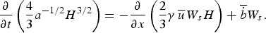 $$\displaystyle{\partial \over {\partial t}}\left( {\displaystyle{4 \over 3}a^{ - 1/2}H^{3/2}} \right) = - \displaystyle{\partial \over {\partial x}}\left( {\displaystyle{2 \over 3}\gamma {\kern 1pt} \overline u {\kern 1pt} W_sH} \right) + \overline {\dot b} W_s.$$
This equation can be rewritten to give
 $$\eqalign{2a^{ - 1/2}H^{1/2}\displaystyle{{\partial H} \over {\partial t}} = & - \displaystyle{2 \over 3}\displaystyle{\partial \over {\partial x}}(\overline u \gamma W_sH) + \overline {\dot b} W_s \Leftrightarrow \cr \displaystyle{{\partial H} \over {\partial t}} = & - \displaystyle{2 \over {3W_s}}\displaystyle{\partial \over {\partial x}}(\gamma {\kern 1pt} \overline u {\kern 1pt} W_sH) + \overline {\dot b}.} $$


 Open access