Data and methods

To examine the effect of snow, we collected two kinds of ice core at each sampling time, with the exception of the 06:00 sampling: one on the snow-covered area (natural conditions) and the other on the nearby bare ice area (2 m × 2 m) which was made by removing snow on ice at 06:00. Immediately after removing an ice core, ice temperatures were measured by drilling holes into the cores and inserting a thermistor probe with accuracy 0.1 K at an interval of 0.05 m to obtain a vertical temperature profile. Snow temperature was measured with the same thermistor at an interval of 0.03 m. To estimate the surface heat budget, the short- and longwave radiative flux was monitored on the intact snow area ~3m away from the sampling site with a radiometer (EKO, MR-40) with an accuracy of 2% at an interval of 1 min. Air temperature and humidity were monitored at the radiometer site at a height of 0.5 m above the snow surface. The collected ice and snow samples were transferred to the cold room (-16°C) after the observation and kept there until ready for analysis. In the cold room, each ice core was split lengthwise into two pieces: one was used for the thin- and thick-section analysis, while the other was cut into a vertical section and segmented every 0.05 m to obtain vertical profiles of density, salinity, brine volume fraction, and δ¹⁸O. The ice density was determined from the weight and dimensions of each segment with an estimated accuracy of ~1%. The S¹⁸O and salinity were measured for the melted ice segment with a mass spectrometer (DELTA plus) and a salinometer (TOWA Electronic Industry, Model SAT-210), respectively. The accuracy was 0.02% for δ¹⁸O and <0.05 psu for salinity. The brine volume fraction was calculated with ice temperature, density and salinity from the formula of Reference Cox and WeeksCox and Weeks (1983). Thin (<1 mm) and thick (5 mm) sections were analyzed to observe the crystallographic alignments with crossed polaroids and the structure of inclusions with scattered light, respectively.

Heat budget calculation

Using the in situ measurements, the heat budget at the surface and inner ice layers was calculated with a thermodynamic ice model similar to Reference Maykut and UntersteinerMaykut and Untersteiner (1971, hereafter referred to as M&U) and the following assumptions:

1. 1. Vertical heat transport is predominant.

2. 2. The bottom of the sea ice is kept at the freezing point of sea water (-1.8°C).

3. 3. A flux toward (away from) the surface is taken to be positive (negative).

In the calculation, the 3 hourly ice and snow temperatures were interpolated onto an hourly grid, and the hourly heat budgets were estimated for the snow layer and each 5 cm thick layer of sea ice from the following equations:

for the snow layer,

for the top layer of bare ice,

and for the other layers in sea ice,

where FSW, FLW, FSH, FLH and FCI are the net shortwave radiation, net longwave radiation, sensible heat flux, latent heat flux and conductive heat flux at the surface, respectively. μ _s, μ _si, T, k _si, h and z are the extinction coefficients of snow and sea ice, temperature, thermal conductivity of sea ice, layer thickness (5 cm) and depth, respectively. For the FSW, the observed values (FSW ↓ - FSW ↑) were used for snow-covered ice while FSW ↓ (1 - α) was given for bare ice, where a is the surface albedo of bare ice and set to 0.5 (Reference Perovich and LepparantaPerovich, 1998). μ _s and μ _si are set to be 20 m^-1 (Reference MellorMellor, 1977) and 3 m^-1, respectively (Reference Maykut and UntersteinerMaykut, 1986). For the FLW, the observed values were used for both snow-covered ice and bare ice because the difference in the surface conditions has little effect on FLW↑. FSH and FLH were calculated by the bulk method. FSH was given by ρ C_p C_su(T _a - T _s), where T _a is the observed air temperature, ρ is the air density (1.3 kg m^-3), C_p is the specific heat of the air (1004J kg^-1 K^-1), C _s is the transfer coefficient for sensible heat and u is the observed wind speed. FLH was given by 0.622ρL_VC _e u(re _sa - e _sS)/p, where L _V is the latent heat of sublimation (2.84 × 10⁶J kg^-1; Reference YenYen, 1981), C _e is the transfer coefficient for latent heat, r is the observed relative humidity, p is the surface pressure and e _sa and esS are the saturated vapor pressure in the atmosphere and at the surface, respectively. The dependence of e_s on air temperature is expressed as a fourth-order polynomial developed by Reference MaykutMaykut (1978). The values of p and u were obtained from the nearest automatic weather station (run by the Japan Meteorological Agency (JMA)) at Tokoro, located ~5 km away from Lake Saroma (Fig. 2). C _s and C _e were taken to be 1.37 × 10^-3 after Reference Andreas and MakshtasAndreas and Makshtas (1985) on the assumption of neutral stability of the air in the atmospheric boundary layer. FCI was calculated from -k(∂ T/∂z), where the thermal conductivity k was calculated from k _s = 2.22362(ρ_s)^1,885 (Wm^-1 K^-1) for snow (Reference YenYen, 1981) and from the empirical formula, k _si, given as a function of the thermal conductivity of brine and pure ice including air bubbles by Reference YenYen (1981) for sea ice.

To estimate the degree of internal melting which has progressed from the initial state in each layer, we introduced the following parameter as a melt progression index:

where FQ is given by Eqns (1), (2) or (3), and Q and M _si are the specific latent heat of fusion and the mass of sea ice at each level, respectively. Q is given by (Reference OnoOno, 1968):

where S _i and T are salinity (psu) and temperature (°C) of sea ice at the initial state. The denominator of Eqn (4) is the total heat required to melt the entire mass, while the numerator is the heat storage accumulated from the initial state. The reason for defining this parameter was to reduce the bias of the ice conditions at the initial stage and examine the intense internal melting layer explicitly. Because Q tends to have a larger value when the temperature is lower at the initial stage, the summation of FQ is not necessarily a good indicator of the progress of internal melting with respect to ice strength.

Results and discussion

For snow-covered ice, the temporal evolution of the vertical profiles of temperature, salinity, brine volume fraction and δ ¹⁸O are shown in Figure 3. Figure 3a shows that whereas a snow layer with low heat capacity and thermal conductivity protected the underlying ice layer from significant warming, the temperature in the snow layer increased significantly and eventually produced a C-shaped profile in the afternoon. In Figure 3b, the prominent increase of salinity in the snow layer during daytime is attributed to the infiltration of tidewater flooding through some cracks (high tide occurred there at 11:05 with amplitude of ~0.3 m). The slight increase of ice temperature and salinity resulted in some increase in brine volume fraction throughout (Fig. 3c). Since the brine volume fraction ranged from 5% to >20% and was always above the threshold of permeability (5%;Reference Golden, Ackley and LytleGolden and others, 1998), the brine network in the sea ice seemed to be permeable. Thin-section analysis with the S¹⁸O data showed that all layers of the sea ice were composed of granular ice originating from sea water.

Fig. 3.

Temporal evolution of the vertical profiles of (a) temperature, (b) salinity, (c) brine volume fraction and (d) d18O for snow-covered ice, observed in Lake Saroma on 20 February 2009.

Based on these data, the individual heat flux was calculated for each ice layer. The time series of FQ, FCI and FSW show that at all levels the temporal evolution of FQ (-30 to 50 W m^-2) was governed by FCI (-30 to 50Wm^-2), and FSW (less than a few Wm^-2) had little effect. Neither net longwave radiation nor turbulent heat flux at the surface (mostly less than ±10 W m^-2) had a significant effect on FQ. The result obtained in the 0-5 cm layer, where the internal melting occurred, is shown in Figure 4. Here the downward FCI essentially controlled the heat-flux convergence FQ. As FQ began to increase at 13:00, MPI also increased significantly in this layer. This result indicates that the temperature profile, especially the positive gradient near the surface, is the controlling factor for the internal melting of sea ice.

Fig. 4.

Time series of FQ, FCI, FSW and MPI at the 0–5 cm layer for snow-covered ice, estimated from the observational results in Figure 3.

Intense internal melting in the 0-5 cm layer is evidenced in the evolution of the δ¹⁸O profiles. Figure 3d shows a significant increase of δ¹⁸O by 0.8% in the top layer (05 cm) after MPI increased. Since pure ice has a higher δ¹⁸O value (>0%_o) than either sea water (-1.25%) or snow (<-5%_o) due to isotopic fractionation during freezing and there is no fractionation on pure ice melting (Reference Jouzel and SouchezJouzel and Souchez, 1982), the increase in δ¹⁸O indicates that the brine in sea ice was replaced by the meltwater from pure ice, as suggested by Reference TisonTison and others (2008). Besides, it was shown from the thin-section analysis that the mean grain size in the 0-5 cm layer increased from 0.9 mm at 06:00 to 1.4 mm at 18:30, whereas it remained almost the same in the other layers. This enlargement of grain size may be explained by the refreezing of partially melted grains while the ice core was kept in the cold room.

For bare ice, the temporal evolution of the vertical profiles of temperature, salinity, brine volume fraction and δ¹⁸O is shown in Figure 5. Figure 5a and b show a more prominent increase of both temperature and salinity in sea ice compared with those for snow-covered ice. The temperature increase can be explained by the penetration of solar radiation, as is shown later, while the salinity increase seems to have been caused by tidewater flooding in the daytime. It is likely that in the absence of snow, flooded sea water infiltrated directly into the underlying ice from the surface. In addition, the increase in porosity in the top layer (Fig. 5c) might have favored infiltration. This also explains the significant decrease in δ¹⁸O in the 0-10 cm layer, in contrast to the case of snow-covered ice (Fig. 5d).

Fig. 5.

Temporal evolution of the vertical profiles of (a) temperature, (b) salinity, (c) brine volume fraction and (d) δ¹⁸O for bare ice, observed in Lake Saroma on 20 February 2009.

The calculated heat flux shows that FQ had the highest value in the 0-5 cm layer (30-50 W m^-2), followed by that in the 5-10 cm layer (0-15 Wm^-2) and in the deeper layers (-5 to +10 Wm^-2). Accordingly, MPI in the 0-5 cm layer increased from 0% at 09:00 to 7.5% at 18:00. We note that in this layer the contribution of FSW (30-40 Wm^-2) to FQ (20-60Wm^-2) was comparable with or slightly larger than that of FCI (20-40 Wm^-2) in the daytime, as indicated by previous results (e.g. Reference Ishikawa and KobayashiIshikawa and Kobayashi, 1985). The net longwave radiation and turbulent heat fluxes contributed to slightly cooling the surface layer (-10 to 0Wm^-2). To contrast FSW with FCI in the inner layer, the time series of FCI and FSW in the 5-10 cm layer are shown with FQ and MPI (Fig. 6). FCI made a negative contribution to FQ in this layer. Therefore, as FSW diminished, FQ was gradually reduced and eventually became negative in the late afternoon. The evolution of MPI was mostly dependent on FSW and increased from 0% at 09:00 to ~2% at 18:00.

Fig. 6.

Time series of FQ, FCI, FSW and MPI in the 5–10cm layer for bare ice, estimated from the observational results in Figure 5.

Thus it was shown from the heat budget analysis of the field observation that for snow-covered ice the convergence of FCI is essential to the internal melting, especially near the ice surface, in contrast to the case of bare ice.

Apparatus and experimental procedure

We prepared a thermally insulated cylinder tank (inner dimensions of 0.38 m diameter and 0.80 m height) and filled it with natural sea water collected from the Sea of Okhotsk (32.5 psu) to 0.75 m depth (Fig. 7). The tank, made from a transparent acrylic, is 0.01 m thick and covered with a 0.1 m thick layer of Styrofoam (except the upper surface) to avoid the freezing on the side wall and the bottom. In order to monitor the ice/water temperature, we prepared copper- constantan thermocouples and mounted them on the side wall at vertical intervals of 0.5 cm for the 0-4 cm layer from the water surface, 1.0 cm for the 4-10 cm layer, and 2.5 cm for the 10-25 cm layer. The room temperature was monitored on top of the tank with another thermometer. These temperature data were logged at 1 min intervals. In order to monitor the sea-water salinity, we made a small hole on a side wall of the tank at 0.4 m depth and stuffed it with a rubber stopper, through which water samples were taken carefully with an injector. As for ice thickness, a measuring scale was put on the side wall and the thickness was measured visually. Water sampling and ice thickness measurement were conducted together at intervals of 6 hours during freezing and 4 hours during melting.

Fig. 7.

Apparatus of the tank experiment. The tank was covered with 0.1m thick Styrofoam to avoid freezing at the side wall and bottom. The copper–constantan thermocouples were mounted on the side wall to monitor the temperature profile. The right-hand panel shows the measurement depths.

Before starting this experiment, the tank was cooled uniformly to a room temperature of -1°C in a cold room, with the water occasionally stirred. After the water temperature settled down to the near freezing point, we set the room temperature at -18°C and began to grow sea ice. When the ice thickness reached ~0.12m, we raised the room temperature to 5°C (hereafter referred to as the melt onset) and examined the evolution of temperature profiles and textural structure until 36 hours after the melt onset (hereafter we refer to the time xxhours after the melt onset as Txx). In order to see the evolution of ice structure, we cut out a rectangular ice block with a basal area of 0.2 m × 0.2 m using a portable saw. Since the condition in the tank was significantly disturbed once the block was removed, we needed to repeat the same experiment seven times under the same conditions to collect the ice blocks at T00, T04, T08, T12, T16, T20 and T24.

Immediately after collecting the ice block, we transferred it to another cold room of -16°C and divided it into four sections with a basal area of 0.1 m × 0.1 m: one was used for thick/thin-section analysis to see the textural structure, two for the measurement of ice density, salinity and δ¹⁸O, and the last one was archived. Among these procedures, thick- section analysis was done first to minimize the refreezing of melted water. The other sections were kept in the cold room until ready for analysis. The method of analysis for ice density, salinity and δ¹⁸O is the same as that described in the previous section except that the vertical resolution was set to 0.02 m. The vertical profile was determined by taking the average of the result obtained from the two sections. With temperature, salinity and density data, brine volume fraction was calculated using the formula of Reference Cox and WeeksCox and Weeks (1983) at each depth. Flexural strength, σ_f , was calculated with the brine volume fraction using (Reference Timco and O’BrienTimco and O’Brien, 1994):

The heat budget, FQ, within the sea ice was estimated every minute at each 1 cm thick layer from

where k _si is the thermal conductivity given as a function of temperature and salinity by Reference YenYen (1981), and ∂T/∂z was calculated from the temperature profile approximated by the fifth-order regression of T with respect to z, fitted to the observed data with a least-square method. Since k _si was estimated to be almost constant (~2.0W m^-1 K^-1) during the experiment, it had minimal impact on the result.

Results and discussion

The time series of ice thickness and temperature over the course of the experiment are shown in Figure 8. Both the thickness and sea-water salinity increased almost linearly with time during freezing. It took 60hours until the ice thickness got to 0.12 m, corresponding to a growth rate of 5 cm d^-1. The salinity increase was 4.5 psu (from 32.5 psu to 37psu), corresponding to a decrease in the freezing point only by 0.2°C. Figure 8 shows the fluctuation in room temperature caused by the mechanism of the air-conditioning system, which had an amplitude of 1.5°C and a 20 min period. However, since the observed ice temperature varied on a much longer timescale, it is unlikely that this fluctuation significantly affected the ice structure. Surface ablation began to occur at T08 and it amounted to ~2 cm by the end of the experiment. A bottom accretion of ~1 cm occurred even after the melt onset.

Fig. 8.

Time series of ice thickness and ice temperature at each depth during the experiment. The depths of ice temperature are 0.0, 0.5, 1.0, 1.5, 2.0, 2.5, 3.0, 3.5, 4.0, 5.0, 6.0, 7.0, 9.0 and 10.0 cm from the ice surface.

Figure 9 shows the evolution of the profiles of temperature, salinity, brine volume fraction, δ¹⁸O, brine salinity and flexural strength in sea ice after the melt onset. Brine salinity, S _b (psu), was calculated from

Fig. 9.

Evolution of the vertical profiles after the melt onset during the experiment for (a) temperature, (b) salinity, (c) brine volume fraction, (d) δ¹⁸O, (e) brine salinity and (f) flexural ice strength. Note that δ¹⁸O is represented by the difference from the initial value of δ¹⁸O of sea water because it varied due to fractionation by repeating the experiments.

(Reference Frankenstein and GarnerFrankenstein and Garner, 1967), where T _i is ice temperature (°C). The characteristic of the temperature profile in Figure 9a is such that with the increase of the surface temperature, the temperature gradient near the surface became positive. Nonetheless, since a negative temperature gradient was maintained near the bottom, a C-shaped profile was produced until T12. Such a temperature profile (i.e. conductive heat flux) explains the slight bottom accretion even after the melt onset (Fig. 8). This phenomenon is attributed to thermal hysteresis peculiar to sea ice which has been previously observed in Arctic perennial ice during the melt season (e.g. Reference Perovich, Elder and Richter-MengePerovich and others, 1997).

The evolution of the salinity profile progressed in three stages (Fig. 9b). Initially, it took a C-shape typical of first-year ice. At the first stage, with the increase in surface temperature, the salinity in the 0-4 cm layer decreased significantly while the salinity in the 4-12 cm layer was nearly stable until T08. At the second stage, the salinity in the 4-12 cm layer decreased significantly while the salinity in the 0-4cm layer remained almost unchanged at T12. At the third stage, the salinity in the 2-6 cm layer decreased slightly while the salinity in the 6-12 cm layer was almost stable at T24. It is probable that the decrease in salinity in the upper layer was affected by the percolation of the melted water produced at the surface (Fig. 8).

These stages can be explained by the evolution of the brine volume fraction (Fig. 9c) and brine salinity (Fig. 9e) profiles. Initially the brine salinity profile had a linearly increasing trend with depth, indicating a potential density instability within the brine network. With the increase of brine volume near the surface, the brine network was interconnected at the 0-4 cm layer, which favored the high- salinity brine flowing down through the network to ~4cm depth. At this stage, the brine density profile was still somewhat unstable (Fig. 9e). At the second stage the brine volume fraction at the lower depth also increased enough for the high-salinity brine water to drain to the underlying sea water, which promoted the desalinization in the lower part of ice. At the third stage the brine density profile became stable, so the desalinization rate slowed down. This result is consistent with that of Reference TisonTison and others (2008).

This process is also related to the evolution of flexural strength determined by the brine volume fraction (Fig. 9f). During the first and second stages when the desalinization was due to the surface melting, the flexural strength decreased at a relatively high rate. However, at the third stage after the desalinization had settled, the decreasing rate of flexural strength slowed down.

Next we examine the evolution of internal melting from the heat budget calculation. Figure 10a shows the evolution of FQ until T36. At a very early stage (T02), the local maximum appeared at 4cm depth when the C-shaped profile was produced. However, as the surface temperature increased rapidly after T04, the maximum FQ shifted to the surface. With the subsequent increase in MPI at the surface, the surface ablation progressed for the period T08-T16 (Fig. 10b). Then, with an increase in the subsurface temperature, the maximum FQ migrated from the surface to the inner depth. This was 5 cm at T24 and 6cm at T36 (Fig. 10a), and the MPI gradually increased in the inner depth as well (Fig. 10b).

Fig. 10.

Evolution of the vertical profiles after the melt onset during the experiment for (a) convergence of conductive heat flux (FQ) and (b) MPI.

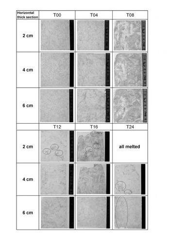
The result of heat budget calculation is supported by the evolution of δ¹⁸O profiles and the thick-section analysis. In Figure 9d, a significant increase in δ¹⁸O is found at the upper 4cm until T16 when a large value of FQ was estimated near the surface. It is likely that brine with lower δ¹⁸O was replaced by meltwater from pure ice, with higher δ¹⁸O associated with gravity drainage of brine, as shown in the field observations. During the same period, it was shown from the thick-section analysis that the porous structure at 2 cm depth became prominent (Fig. 11). Afterwards at T24, when the maximum FQ shifted downward, the porous structure also migrated to the lower depth, which is consistent with the fact that MPI increased significantly up to ~40% at 5 cm depth.

These results indicate that the conductive heat flux is a controlling factor of internal melting and the estimation of FQ and MPI coincided with the evolution of the inner ice structure. These processes can be represented by the time series of the total MPI and ice flexural strength (Fig. 12). Consequently, from the laboratory experiment the melting process is summarized as follows:

1. 1. As the surface temperature increases, the C-shaped temperature profile appears and FQ reaches a maximum in the subsurface layer. But this stage lasts only for a short time and has little effect on the ice structure. (T02)

2. 2. With the further increase of the surface temperature, the maximum FQ shifts to the surface and induces significant melting in the top 4cm layer. Associated with this, the total flexural strength reduces rapidly (Fig. 12). Since the initial brine density profile is unstable, this melting induces desalinization that releases the gravitational energy in this layer. However, desalination at this stage is limited to the upper layer because of the relatively low brine volume fraction across the lower layers. (~T08)

3. 3. Next as MPI increases in the lower layers, it promotes the flow of brine through the brine network, which leads to substantial desalinization. Since the internal melting remains high near the surface, the total flexural strength continues to be reduced. (~T16)

4. 4. Through stage 3, the brine density profile becomes stable and so the desalinization becomes moderate. Concurrently, the maximum FQ shifts from the surface to the inner depth again and increases MPI at the lower depth (Fig. 12). In this way the intense internal melting migrates downward. However, at this stage the increase in total FQ is reduced and the rate of decrease in the ice flexural strength eases (Fig. 12). (~T24, T36)

   Here it should be noted that the values of FQ estimated in the laboratory experiment, 0-80 Wm^-2, were somewhat larger than those (0-50Wm^-2) estimated in the field observation. Therefore, to check the above result, we also carried out a repeat experiment, but at a room temperature of 3°C during the melting. In this case, FQ in the top layer was reduced to 10-60Wm^-2, which is closer to the observational values. Thus, overall we find the above process holds true except that the progress slowed by a few hours.

   Fig. 11.

   Evolution of the internal ice structure observed from the horizontal thick section at depths of 2, 4 and 6 cm, showing the formation of porous structure after T12.

   

   Finally, we discuss the applicability to snow-covered ice. In this experiment where bare ice was used, the maximum of FQ and MPI was shown to linger for many hours at the surface at stages 2 and 3. This is attributed mainly to the salient increase of surface ice temperature. For snow-covered ice, however, the increase in ice surface temperature is expected to be reduced due to the presence of snow (compare Fig. 3a with Fig. 5a). In this case, we infer that the value of FQ at the ice surface would be somewhat reduced and the maximum of FQ would migrate downwards faster before substantial melting occurs at the surface, as demonstrated by Tison and others (2008, Fig. 5). The migration speed would depend on the duration of the warming by the external forcing. If the maximum FQ lingers at a certain depth, it would be possible that internal melting occurs intensively there, as observed by Abe (2007;Fig. 1).

   Fig. 12.

   Time series of MPI at each depth and total flexural ice strength, estimated from laboratory experiment.

   

Formulation of the model

Since our method for calculating the heat budget, based on M&U, came close to representing the evolution of sea-ice structure in both the field observation and tank experiment, we adopt the same method here. In the model, sea ice is assumed to be a horizontally uniform slab of 0.35 m thickness with a 0.05 m snow cover, following the observational result in Lake Saroma. Since this thickness value is close to that of undeformed first-year ice in the southern Sea of Okhotsk (Reference Fukamachi, Mizuta, Ohshima, Melling, Fissel and WakatsuchiFukamachi and others, 2003; Reference Toyota, Kawamura, Ohshima, Shimoda and WakatsuchiToyota and others, 2004) and in the Indian sector of the Antarctic Ocean in winter (Reference Worby, Geiger, Paget, Van Woert, Ackley and DeLibertyWorby and others, 2008), the result will be applicable to the wide area of the SIZ. Unlike M&U, it is assumed that there is no snowfall, accretion or ablation of sea ice during the period. This assumption is valid because in this study we focus on a relatively short period in the melt season. The temperature within snow and sea ice is governed by the following one-dimensional heat equation:

for snow temperature

and for ice temperature

where P, C, T, H and k are the density, specific heat, temperature, thickness and thermal conductivity, respectively, and subscripts s and si denote snow and sea ice, respectively. The constant values are set to ρ_s = 400kgm^-3, ρ_si = 900 kg m^-3 and H _s = 0.05 m from the observations. The specific heat of snow, C _s, is given as a function of temperature from Reference MellorMellor (1977), and the specific heat of sea ice, C _si, is given as a function of temperature and salinity from Reference OnoOno (1968). FSW_net is the net solar radiation absorbed at the snow surface, given by (incoming solar radiation) x (1 - α), where snow albedo α is set to 0.8. FSW_in is the solar radiation penetrating into the sea ice and expressed as FSW_net exp (-μz), where μ is an extinction coefficient and is set to be 20 m^-1 for snow and 3 m^-1 for sea ice. FLW_in is incoming longwave radiation and is estimated by 0.7855(1 + 0.2232C^2,75)σT _a ⁴, where C is the cloud fraction in tenths, σ is the Stefan-Boltzmann constant, and T _a is air temperature, from Reference Maykut and ChurchMaykut and Church (1973). Outgoing longwave radiation FLW_out is given by εσT _s ⁴, where ε is emissivity of snow and set to 0.99. FLH and FSH are calculated from the same formulas that were used in the field observations. A time-step At and grid spacing Δz are set to 0.5 hour and 0.05 m, respectively. From Eqns (6) and (7), the temperature at the ith layer and the nth time-step, T (n, i), is calculated by the following equations: for snow layer

for ice layer

where i = 1 and i = 2-8 correspond to the snow layer and the ice layers, respectively. The initial temperature and salinity of sea ice were given by the values observed on-site for the 0.35 m thick ice at 06:00 on 20 February 2009 (courtesy of Mika Makela). We assume that the vertical profile of salinity within the ice remained unchanged over the entire period. Although in reality the salinity profile varied due to desalination processes and the tidewater flooding (Fig. 3b), it is quite difficult to predict these events, and the effect is not important because the sensitivity of physical parameters to salinity is relatively small (Reference OnoOno, 1968). As for the upper boundary condition, whereas M&U calculated the surface temperature by assuming that all the fluxes are balanced at the surface, in this study T _s was determined by Eqn (8). This was necessary because our time-step (Δt =0.5 hour) is shorter than for M&U (Δt =12 hours), so the assumption that the fluxes are balanced may not necessarily be valid in our case. The meteorological data required to calculate the fluxes in Eqns (8) and (9) were taken from the nearest JMA stations, Tokoro for air temperature and wind speed, and Abashiri for incoming solar radiation, sea-level pressure, vapor pressure and cloud amount (see Fig. 2 for their locations). The lower boundary condition was given by T =-1.8°C at the bottom. Using these data, the integration of Eqns (8) and (9) was performed from 06:00 (LST) on 20 February until 23:30 on 31 March 2009.

Fig. 13.

Evolution of computed temperature profiles on (a) 20 February 2009, (b) 7 March 2009 and (c) 24 March 2009.

Results and discussion

First we validate our model by comparing it with the observational results obtained on 20 February. Figure 13a shows the diurnal variation of the temperature profiles obtained from our model. When compared with Figure 3a, it is found that there was a significant diurnal variation in the observed temperature profile, especially near the surface, and the model reproduced it well. Therefore the model results allow us to confidently examine the evolution of the temperature profile and hence melting processes within sea ice.

The time series of the observed air temperature and the modeled ice temperature at each depth are shown in Figure 14. Although a large fluctuation, including the diurnal variation, is found in air temperature (Fig. 14a), the whole period can approximately be divided into three phases: (1) the pre-melt phase (20-28 February), (2) the early melt phase (1-20 March) and (3) the mid-melt phase (21-31 March). During phase 1, the average temperature is about -5°C, ranging from -10 to 0°C, while during phase 3 the average is ~0°C, ranging from -5 to +5°C. Phase 2 corresponds to the transition between these two phases. The ice temperature profiles reflect the evolution of air temperature (Fig. 14b). During phase 1 the negative vertical gradient was maintained although the diurnal variation was seen near the surface. During phase 2, the negative vertical gradient was reduced and the upper layer temperature sometimes exceeded the inner temperature, suggesting the formation of the C-shaped profile. During phase 3, the temperature within the sea ice became almost homogeneous at the freezing point.

This feature is visualized by the diurnal variation of the temperature profile on a specific day in Figure 13. The temperature profiles are characterized by a negative vertical gradient with significant diurnal variation near the surface during phase 1 (Fig. 13a), the C-shaped figure with still large diurnal variation near the surface during phase 2 (Fig. 13b) and an almost homogeneous or even slightly positive gradient with reduced diurnal variation during phase 3 (Fig. 13c). The decrease in the diurnal variation of ice temperature with time is attributed mainly to the property that the specific heat of sea ice increases significantly with the increase in ice temperature (Reference OnoOno, 1968). The comparison between temperature profiles at each phase suggests that, especially during the early melt season (phase 2), the convergence of conductive heat flux FCI plays an important role in the internal melting process.

Fig. 14.

Time series of (a) air temperature observed at the Tokoro JMA station, and (b) the ice temperature at each level calculated from numerical modeling. Dates are month/day in 2009.

This is confirmed by the heat budget analysis. Figure 15 shows the contribution of FCI and FSW at each depth, averaged for each phase. During phase 2, FCI dominates the warming, especially near the surface, and the contribution of FSW is much less. In this phase, as time progresses, the convergence of FCI gradually migrated downward, so the internal melting propagated to the lower depths. This feature contrasts with the results obtained for phases 1 and 3. During phase 1, FCI instead contributes to cooling except in the surface layer (Fig. 15a), and during phase 3 the contribution of FCI was reduced and almost comparable with that of FSW (Fig. 15c).

Associated with the evolution of the internal melting, ice flexural strength also changed significantly. Figure 16 shows the time series of the total MPI and ice flexural strength. MPI, which remained low during phase 1, increased significantly at all depths during phase 2. Accompanying this MPI increase was a significant decrease in the ice flexural strength. It is noticeable that, at the end of phase 2, MPI in the 15-20cm layer surpassed that in the upper layer, suggesting the intense internal melting there. In phase 3, the MPI increase became moderate, so the ice flexural strength became relatively stable. This property is similar to that obtained in the tank experiment (Fig. 12).

Therefore the early melt season plays an important role in decreasing flexural ice strength, most significantly due to the characteristic C-shaped temperature profile. This is consistent with the result of Reference JohnstonJohnston (2006) in that ice strength shows a stepwise decrease according to the evolution of brine volume during the melt season.