2.1 Definition of steady-state and anomalous motions

The effect on glacier motion of changes in sliding velocity is most simply examined by separating the added anomalous motion u(x, t) caused by a specific anomalous sliding-velocity distribution from a steady-state motion u ₀(x) that would occur without the anomaly. The velocity anywhere in the glacier is then expressed as u ₀(x) + u(x, t).

The steady-state velocity distribution u ₀(x) and the corresponding stress distribution σ ₀(x) satisfy the field equations for flow under the action of gravity, with atmospheric pressure at the upper surface and the steady sliding u ₀(x _b) at the bed. The sum of the steady-state and anomalous distributions must also satisfy these field equations, with the boundary conditions changed to include the additional anomalous sliding velocity u(x _b, t).

2.2 Geometrical assumptions and coordinate system

Planar slab geometry is assumed. Coordinates are chosen as shown in Figure 1, with the x-axis on the upper surface and positive down the slope, the y-axis normal to the surface and positive towards the bed, and the z-axis horizontal across the slope. The steady-state velocity distribution u ₀(x) is assumed to be compatible with planar geometry and a constant ice thickness H, under a prescribed mass-balance distribution. The anomalous motion is assumed to be planar: the x and y components of velocity u and v may be non-zero functions of x, y, and t, but anomalous motion across the slope in the z direction is everywhere zero.

Fig. 1.

Definition of geometrical quantities and coordinate system.

This paper is concerned with the instantaneous velocity distribution at a specified time and for a specified planar geometry. A more complex and less well-defined problem would be the subsequent evolution of the geometry and velocity. Any basal velocity anomaly is likely to cause an anomalous normal velocity at the upper surface and gradually change the geometry of the glacier. This geometry change would feed back to affect the velocity distribution (Reference Langdon and RaymondLangdon and Raymond, 1978; Reference HutterHutter, [^c1983]; Reference Kamb and EchelmeyerKamb and Echelmeyer, in press). If the time-scale of interest is short, or the velocity anomalies are small compared to the steady-state velocity u ₀, then the geometry changes and corresponding velocity changes may be negligible. Under these restrictive conditions the problem of the eventual evolution of the surface geometry does not arise.

2.3 Rheological assumptions and field equations

The ice is assumed to flow as a Newtonian fluid of uniform dynamic viscosity η. The relevant field equations are the equation of continuity for incompressible flow, and the Navier–Stokes equations. Velocity anomalies are assumed to vary slowly enough that acceleration terms are negligible. From the assumptions that the motion is planar and that the steady-state distributions u ₀ and σ ₀ satisfy the equations with body force from gravity, standard considerations yield the following field equations for the velocity-anomaly components u and v, and the anomalous pressure p:

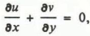
The gravity body force does not appear in these equations because the steady-state stress distribution σ ₀ is in static equilibrium with gravity, and the linearity of the equations results in the anomaly fields being independent of and additional to the steady-state distribution.

2.4 Boundary conditions

The boundary conditions to be applied are atmospheric pressure on the upper surface and a prescribed velocity at the base. At the upper surface the steady-state distributions u ₀ and σ ₀ correspond to atmospheric pressure. The additional stress on this surface from the anomaly distributions u and σ must therefore be zero. For the given coordinate system this is expressed as

keeping in mind the restrictions on the geometry of the upper surface discussed in the previous section. At the base, a prescribed velocity anomaly is expressed as

Equation (5a) is appropriate to slip along a flat base, and Equation (5b) allows for a simple approximation of the opening and closing of cavities.

A physically based sliding law relating basal velocity to basal stress, with spatially or temporally varying parameters, could also be used instead of Equation (5a), From a physical point of view, this would be a more direct approach to the origin of the basal velocity anomalies. From an observational point of view, it is better to relate surface velocity directly to basal velocity, especially since in practice a realistic sliding law is not known. The mathematical formulations for these two approaches are somewhat different. However, except possibly for cases involving mathematical singularities, the results of one formulation could be interpreted in terms of the other.

2.5. Solution technique

Equations (1) to (3) are solved using a stream function ψ such that

Equation (1) is trivially satisfied for any choice of ψ. Substitution of Equation (6) into Equations (2) and (3) gives two corresponding equations for ψ and p. Differentiation of Equation (2) with respect to y and Equation (3) with respect to x and the requirement ∂² p/∂x∂y = ∂² p/∂y∂x implies that ψ must be biharmonic, that is

Furthermore, when ψ is biharmonic, p can always be found from a path-independent integration of Equations (2) and (3). Thus the solution of Equations (1) to (3) is reduced to the solution of Equation (7).

To solve Equation (7), the boundary conditions in Equations (4) and (5) must be expressed in terms of ψ. Treatment of Equation (4a) is simplified if it is equivalently expressed as ∂σ _yy (x,0,t)/∂x = 0, plus the requirement that at some point on y = 0, σ _yy = 0 (e.g. σ _yy (0,0,t) = 0). In this differentiated form of Equation (4a), ∂p/∂x and ∂² v/∂x∂y can be calculated in terms of ψ from Equations (2) and (6) to find

Substitution of Equation (6) into Equations (4b), (5a), and (5b) gives

2.6 Some properties of solutions

Because of the linearity of Equations (1) to (3) or equivalently Equation (7), it is apparent that if ψ^(a) and ψ^(b) are solutions, then ψ = ψ^(a) + ψ^(b) is also a solution. Furthermore, if ψ^(a) and ψ^(b) satisfy the boundary conditions in Equations (8) and (9) corresponding to u _b ^(a) and u _b ^(b) in Equation (9a) and v _b ^(a) and in Equation (9b), then ψ also satisfies the boundary conditions with u _b = u _b ^(a) + v _b ^(b) and v _b = v _b ^(b) + v _b ^(b). This expresses the well-known principle of superposition of solutions. It is also evident that if v _b = 0, so that ψ is a solution corresponding to a basal velocity u _b, then ∂ψ/∂x is also a solution and corresponds to a basal velocity ∂u _b/∂x. These properties can be used to generate new solutions from existing ones.

Another important property of the equations is that they depend on time only through boundary conditions in Equations (9a) and (9b). This arises because of the assumed fluid rheology and the absence of acceleration terms, so that the internal flow responds to the basal boundary condition without time lag. An important consequence of this is illustrated by the following example. Suppose v _b = 0, so that ψ(x,y) is a solution corresponding to u _b(x), then a(t)ψ(x) - wt, y) is a solution corresponding to a(t)u _b(x − wt). Thus a solution for a certain time-independent, fixed spatial distribution can easily be modified to give a time-varying amplitude, or a propagating solution of the same wave shape. The solutions in the following sections will only be written in time-independent form, with the understanding that the corresponding propagating solutions can easily be determined.

Finally, it is noteworthy that the dynamic viscosity η drops out of all of the Equations (7) through (9b) which determine ψ. This arises because there are no prescribed stress-boundary conditions other than the free upper surface, and no body force. In consequence, the anomalous velocity is independent of η and differences in the velocity distribution arise only from differences in the kinematic boundary conditions in Equations (9a)and (9b). However, the anomalous stress distribution will depend on η, although this distribution is not examined explicitly in this paper.

3.1 Harmonic surface-parallel basal velocity anomaly

Suppose the velocity anomaly at the base of the glacier is

where U _b is the amplitude of the basal anomaly. With the given rheology and assumptions, the velocity throughout the ice mass will also vary harmonically. A solution to Equation (7) varying harmonically with x is

Boundary conditions in Equations (8) and (9) give four equations which determine the coefficients A _u, B _u, C_u, and D _u as follows

The velocity anomaly at any point (x,y) can be found from Equations (6), (11), and (12) The surface-parallel component at (x,y) is

and the surface-normal component is

Here

and

The velocities consist of a transfer or filter function multiplying the basal velocity u _b. The surface-parallel velocity component anywhere in the glacier is in phase with the surface-parallel velocity at the base; the surface-normal velocity component is everywhere 90° out of phase from the surface-parallel velocity component.

The velocity-transfer functions evaluated at the surface (y = 0) are

for the surface-parallel velocity component, and

for the surface-normal component.

Schematics of the internal motion for harmonic surface-parallel basal velocity anomalies of a short and a long non-dimensional wavelength λ/H are shown in Figure 2a and 2b. The important difference between these two cases is that for the short wavelength the velocity anomaly recirculates, while for long wavelengths it does not. This leads to interesting effects at the surface; particularly for short wavelengths the surface-parallel component will have an opposite direction at the surface to that at the base. (This can either be viewed as a sign change or a 180° phase shift.) Also, at a certain intermediate wavelength λ/H ≈ 5.2, the amplitude at the surface of the surface-parallel velocity component is zero. At this wavelength the surface amplitude of the surface-normal component reaches its maximum. These effects are summarized in Figure 3.

Fig. 2.

Contrasting patterns of motion represented schematically for harmonic basal velocity anomalies (shown for a half wavelength): (a) basal anomaly u_b, short wavelength (λ/H = 1); (b) basal anomaly u_b, long wavelength λ/H = 10); (c) basal anomaly v_b, short wavelength (λ/H = 1); and (d) basal anomaly v_b, long wavelength (λ/H = 10).

Fig. 3.

Relative amplitudes of surface velocity, caused by harmonic variation in basal velocity (of unit amplitude). Solid line, T_uus; dashed line, T_vvs; short dashed line, T _uvs = T _vus.

3.2 Harmonic surface-normal basal velocity anomaly

Now suppose that the velocity anomaly at the base of the glacier is

where V _b is the amplitude of the basal anomaly. A solution to Equation (7) then is

Using boundary conditions in Equations (8) and (9), the coefficients A _v , B _v , C _v and C _v are found to be

The resulting velocity anomaly at a point (x,y) is

and

where

and

The velocity-transfer functions evaluated at the surface (y = 0) are

for the surface-parallel velocity component, and

for the surface-normal component.

Comparison of Equation (21a) with Equation (15b) shows that T _vus = T _uvs , i.e. the “cross-component” transfer functions are equal at the surface.

Schematics of the flow for harmonic basal surface-normal anomalies of a short and a long non-dimensional wavelength are shown in Figure 2c and d. The major difference is that the amplitude of the surface velocity is greater for the longer-wavelength anomaly. The amplitudes at the surface of the surface-parallel and surface-normal components also vary relative to each other depending on the wavelength, although not in a significant manner for the schematics shown. These effects are summarized in Figure 3.

3.3. Fourier transform solution

The Fourier-transform method theoretically allows surface solutions to be found for any pattern of basal velocity u _b and v _b. The Fourier transform and the inverse transform are defined as

Using Equation (22a), the transform of Equation (7) is

A solution for

is

By transforming the boundary conditions (Equations (8) and (9)), the coefficients A, B, C, and D are found, and are most simply written in terms of the coefficients in Equations (12) and (18):

Here û _b(k) is the Fourier transform of the surface-parallel component of the basal velocity anomaly, and

is the transform of the surface-normal component of the basal velocity anomaly. These equations are analogous to those found for a single harmonic component in sections 3.1 and 3.2.

The actual basal anomaly components u _b(x) and v _b(x) must be specified (as two of the boundary conditions). From the transformed basal velocity components û _b and

the transformed stream function is determined using Equations (24) and (25). This is used to calculate the transformed velocities anywhere in the glacier:

If these are written out in terms of the individual coefficients (Equations (25)), then the transformed velocities can easily be rewritten in terms of the transfer functions (Equations (14) and (20)). Then, when evaluated at the sur-face, the transformed velocity components are:

These surface-transfer functions are given explicitly in Equations (15) and (21). T _uvs is used instead of T _vus in Equation (27a), since these two transfer functions are identical.

The Fourier-transform solutions in the following sections were calculated using a discrete Fourier-transform routine. The discrete Fourier transform assumes that the function is periodic. The surface effects of this assumption can be minimized by having a length of at least 2.5H on each side of the region of interest in the basal function (since this is about the maximum distance to which surface effects spread out from the basal function).

4.1 Surface response to basal front

An anomaly in the surface-parallel component of basal velocity that has the form of a front of amplitude (half-height) U _b can be expressed as:

The corresponding surface response can be calculated using Equation (27) and a discrete Fourier-transform routine.

Surface and basal velocities are compared in Figure 4 for such a basal front. The abrupt change in u at the basal front is spread out over about 5H at the surface. Also, the trend of u at the surface is not as smooth as would be expected. Instead, there is a flat of width about 1H in the surface velocity over the basal discontinuity. The flat in the surface-parallel component of the surface velocity occurs because of reverse contributions when the high wave-number Fourier components of u _b are filtered to the surface through the transfer function. These high wave-number components dominate near the basal front, and their reverse surface contributions break the larger-scale trend established by the lower wave-number contributions.

Fig. 4.

Basal and surface velocities for a basal velocity anomaly u_b: a sharp front shown by solid lines, a steep ramp wave (r = 0.025) shown by dashed lines where distinguishable, and a less steep ramp wave (r = 0.1) shown by short dashed lines. Surface-normal velocity is positive upwards.

4.2 Surface response for ramp at base

An anomaly in the surface-parallel component of basal velocity that has the form of a ramp can be written as

The slope of the ramp is −U _b /r, where 2r is the horizontal distance taken up by the ramp.

Basal and surface velocities for r = 0.25H are shown in Figure 4. This produces a ramp in u _b of width 0.5H. At the plotting scale, the calculated surface-velocity components are almost indistinguishable from those for a sharp basal front.

If the basal velocity ramp width is increased, the flat in u _s becomes less prominent, and the maximum amplitude of v _s decreases (see Fig. 4). However, the width of the basal ramp does not noticeably affect the width of the zone of the surface-velocity anomaly, as long as the basal ramp is less than about 5H wide.

4.3 Surface solution for Gaussian peak at base

A pulse in basal velocity is plausible for both the surface-normal and surface-parallel components. An anomaly in the surface-parallel component at the bed which has the spatial form of a Gaussian peak is expressed as

where σ is the standard deviation. The surface effects vary depending on the ratio of the standard deviation of the peak to the thickness of the ice (σ/H). Three results are shown: a wide peak (Fig. 5a), a medium width peak (Fig. 5b), and a narrow peak (Fig. 5c). As the peak is made narrower, u _s develops a dip over the center of the basal peak, and v _s becomes more pronounced. These effects are summarized in Figure 6. The high wave-number terms of the basal velocity are the source of these variations (as was explained in section 4.1).

If a Gaussian pulse is made narrower and taller while holding the area constant in the limit of zero width, it approaches a delta function. The delta-function solution can also be found by differentiation of the solution for a basal front. From this point of view, the dip in surface velocity directly above a basal delta-function spike corresponds to the surface-velocity “flat” above a discontinuous front. The delta-function solution is qualitatively the same as Figure 5c for the narrow Gaussian pulse.

Fig. 5.

Relative basal and surface velocities for Gaussian pulse basal velocity anomalies u_b. with (a) σ/H = 5, (b)σ /H = 0.5. and (c) σ/H = 0.05. Solid line, u_b; dashed line. u_s (where distinguishable from u_b): short dashed line, v_s (positive upward). Basal velocity anomalies integrated over distance equal in all three cases.

Fig. 6.

Charcteristics of u_s in response to Gaussian pulse basal velocity anomalies u_b, and their dependence on the longitudinal scale of the pulse.

The solution for a delta-function anomaly in u _b provides the formal means for expressing the solution for any arbitrary spatial distribution of u _b in terms of a spatial decomposition based on a Green’s function. (A similar solution is possible for a delta-function anomaly in v _b.) Let the surface velocity at position x caused by a unit basal delta function at x′ be expressed as G _s(x, x′) = G _s(x − x′). Figure 5c approximates G _s (x − x′) with x′ = 0. By superposition, the surface solution for an arbitrary spatial distribution of u _b(x,t) is

Since the analytical representation of G _s(x − x′) derived above is very complex, this approach does not seem gener≤ally useful now. If a simple analytical approximation were fitted to G _s (x – x′), then Equation (31) could be very use;ful, but this is not pursued here.

One property of G _s (x – x′) can be used to arrive simply at a useful result. This property is

This can be seen in several ways. For example, the solution for a basal delta function is the x derivative of the solution for a unit basal front at x′. Thus G _s (x − x′) for fixed x′ gives the x derivative of surface velocity for a unit basal front at x′ and, when it is integrated over adequate distance from one side of the front to the other, it gives the total velocity jump at the surface and at the bed (Fig. 4). From Equations (31) and (32)

which shows the integrated velocity is the same at the surface and bed for any basal velocity anomaly.

A Gaussian pulse in the surface-normal component of basal velocity (perhaps caused by cavitation) can be represented as

Surface effects are shown for a wide peak (Fig. 7a), a medium-width peak (Fig. 7b), and a narrow peak (Fig. 7c). The cross-component effects are the same as for the surface-parallel basal anomalies (since T _vus = T _uvs ). The surface-normal component at the surface is reduced in amplitude and increased in longitudinal extent relative to the basal pulse, as the basal pulse is made narrower.

Fig. 7.

Relative basal and surface velocities for Gaussian pulse basal velocity anomalies v_b, with (a) σ/H = 5, (b) σ/H = 0.5, and (c) σ/H = 0.05. Solid line, v_b (positive upward); dashed line, v_s (positive upward): short dashed tine, u_s. Basal velocity anomalies integrated over distance equal in all three cases.

5.1 Longitudinal scales of transfer

Based on the considerations of the foregoing sections, four longitudinal scales of differing behavior may be identified. Basal velocity anomalies of a long scale appear at the surface unattenuated, and deformation-induced cross-component motions are negligible. At an intermediate scale, the surface-parallel and surface-normal velocity components have nearly the same spatial pattern at the surface as at the bed, but with reduced amplitudes. At this scale, cross-component motions caused by ice deformation become noticeable. At a short scale, while the surface-normal component at the surface is reduced in amplitude from that of the basal surface-normal component, the surface-parallel component at the surface is significantly altered in both amplitude and spatial pattern in comparison to that at the bed. At this short scale, cross-component motions are sub-stantial. Finally, there is a very short scale at which there is essentially no response at the surface.

These systematics are best seen with reference to harmonic basal anomalies (Fig. 3) and basal peaks (Figs 5, 6, and 7). The boundary between the four scales can be roughly identified as 10H (long to intermediate), 5H (intermediate to short), and 1H (short to very short). Since the change in behavior with longitudinal scale is gradational, these boundaries cannot be positioned precisely. Furthermore, the positions of the boundaries depend to some extent on the spatial pattern as can be seen from comparison of Figures 3 and 6. Any real pattern of basal velocity variation will likely have features at a variety of scales. A basal velocity front is one example for which there are effects at all of these scales (Fig. 4).

5.2 Deformation-induced surface-normal motions and estimates from surface strain-rate

For intermediate and short scales, Figures 3 and 6 show that a basal velocity anomaly such that u _b ≠ 0 and v _b = 0 causes both u _s and v _s to be non-zero, and v _s may be larger than u _s. From ice continuity (Equation (1)), and assuming v _b = 0, v _s is

If the anomalous surface-parallel motion were independent of depth, then 〈∂u/∂x〉 _H could be found from ∂u _s/∂x measured at the surface. The problem is that in general u is attenuated toward the surface and ∂u _s/∂x will underestimate the magnitude of the average of ∂u/∂x over depth. Furthermore, at the short scale the signs can be opposite. These problems are illustrated in Figure 8.

Fig. 8.

Surface-normal velocity calculated as H∂u/∂x scaled by v_s from mathematical model for harmonic basal velocity anomaly u_b. Solid line, (H∂u_s/∂x)/v_s; dashed line, (H∂u_b/∂x)/v_s. (b) Surface-normal velocity (positive upward) calculated as H∂u_s/∂x (dashed line) compared with v_s from mathematical model (solid line), for a Gaussian pulse basal velocity anomaly u_b with σ/H = 0.05, of maximum amplitude u_b(0) = 10.

5.3 Problems of interpretation of measured surface-velocity and uplift variations

On Variegated Glacier, propagating “mini-surges” occurred quasi-periodically during the early melt seasons for several years prior to the main surge. These were characterized by a zone of accelerated motion which propagated down-glacier at about 0.1–0.6 km h⁻¹. At a given location, speed rose rapidly over a few hours to a sharp peak, dropped rapidly and then more slowly over about 1 d as the zone approached (paper in preparation by B. Kamb and H.F. Engelhardt). Often there was a secondary velocity peak following the first principal one by several hours (Reference Raymond and MaloneRaymond and Malone, in press.)

The surface-parallel velocity anomalies u _s averaged over 1 d were on the order of 0.5–1 m d⁻¹ and resulted in extra anomalous surface displacements of 0.5–1 m over the 1 d interval of a mini-surge. The peaks in u _s were on the order of three to four times larger than the day-averaged values. In addition there was a noticeable anomaly v _s, which produced a relatively rapid uplift rate of up to about 1 m d⁻¹ over one to several hours, followed by a slower more extended subsidence. The maximum uplift was about 0.1 m and occurred after the peak in u _s by 1 or 2 h.

These time intervals and propagation speeds correspond to spatial scale of from about 1 km to more than 10 km, which can be compared to the ice thickness of about 0.4 km. Therefore, the surface-velocity patterns of these mini-surges have features from the small to the large scale.

Figure 9 shows an example constructed from a superposition of ramps and a Gaussian spike for u _b, and a Gaussian pulse for v _b. Surface velocities are shown both with and without the effects from v _b. This example shows some of the qualitative features of mini-surge-velocity variation. Due to the simplifications of the model, it is premature to attempt a detailed inversion of measured surface velocity for calculation of basal velocity. Furthermore, this will in any case not be straightforward, due to the high attenuation between the bed and surface for short wavelengths and an intermediate wavelength interval (about 5H for this model), which causes problems of resolution and accuracy. Nevertheless, some semiquantitative conclusions are possible. The broad-scale asymmetric peak in mini-surge velocity is of long enough scale that it probably resembles in shape and amplitude the actual variation at a similar scale at the bed, except for some broadening of the velocity rise at the surface in comparison to the bed. The narrow principal peak and the sub-sequent secondary peak may be indicative of a single sharp peak at the bed of substantially higher velocity and represent intermediate- to short-scale features. The principal peak at the surface has a half-width of about one depth, which suggests the peak at the bed could be narrower and have a velocity anomaly more than three times that at the surface. Furthermore, the positions of the peak at the bed may be shifted relative to the principal peak at the surface, probably toward the secondary peak. Finally, at this scale the deformation-induced surface-normal velocity component at the surface will have an amplitude similar to the anomalous surface-parallel component at the surface. Uplift determined by integration of v _s when v _b = 0 shows a rapid rise and a subsequent slower fall. The maximum uplift is ≈ 0.13 times the anomalous surface-parallel displacement caused by the passage of the velocity wave; this is seen by comparison of the areas under the positive parts of the v _s and the u _s curves. This shows that a large fraction or possibly all of the surface uplift during mini-surges could be explained by internal deformation without uplift at the bed.

Fig. 9.

Surface velocity components u_s and v_s (upper two solid curves) for a hypothetical basal velocity anomaly with component u_b (lower solid curve). Addition of basal component v_b (lower dashed curve) results in total surface components u_s and v_s (shown by upper two dashed curves). Anomalies propagating with speed w; surface-normal velocity is positive upward.

Reference Iken, Iken, Röthlisberger, Flotron and HaeberliIken and others (1983) have observed variations in surface velocity and elevation on Unteraargletscher at an approximately 4 d time resolution. At this time resolution, they find a correlated velocity increase and uplift of the surface during an approximately 7 month summer season. Several short-term velocity and uplift events lasting more than 4 d are superimposed on it. These short-term velocity variations have some resemblances to the mini-surges of Variegated Glacier; however, little is known about their spatial variation or propagation. Assuming the Unteraargletscher events propagate at speeds similar to or faster than the Variegated Glacier mini-surges, which is consistent with the description of available information, the durations of the features would indicate that these events have large spatial scale and are free from the complexities of the short and intermediate scales in the foregoing analyses. Reference Iken, Iken, Röthlisberger, Flotron and HaeberliIken and others (1983) have carefully considered in detail various possible contributions to the surface uplift and conclude that its major features must arise from the opening of cavities at the bed but, based on limited measurements of surface strain-rate changes, they caution that vertical ice straining could be a major contribution. We emphasize here the possible major errors when using surface values of longitudinal strain-rate to estimate averages over depth unless the spatial scale of velocity variation is well known. Furthermore, unlike a velocity measurement, which represents an average over time, an uplift measurement is a sample at a single time and may not be representative of the time interval over which the velocity has been averaged.

5.4. Limitations of the model

A major limitation of the model is the assumption of a linear viscous fluid rheology to represent ice behavior. Some of the features of the strain-rate pattern during Variegated Glacier mini-surges show dramatic changes on time-scales short compared to the time needed to establish steady-state creep in experiments. This indicates possible visco-elastic effects. This problem has been examined using a linear visco-elastic Maxwell rheology, which gives some difference in behavior in comparison to the purely viscous rheology, but these differences are not major (paper in preparation by M.J. Balise). More importantly, ice creep is better approximated by a power law with power of 3–4 than by a linear fluid (power of 1). This could lead to some substantial differences in behavior. In the limit in which the velocity anomalies induced at the bed and their strain-rate contributions are much smaller than the steady-state velocity and strain-rate, the velocity-anomaly field will occur in a distribution of effective viscosity controlled by the straining associated with the steady-state motions. In this circumstance, a perturbation solution could be attempted (Reference HutterHutter, [^c1983]). The effective viscosity will then tend to be low near the bed and high near the surface (Reference Whillans and JohnsenWhillans and Johnson, 1983). This will tend to promote recirculation of the velocity anomaly near the bed and probably increase the length for transition between the short and intermediate scales described above. If the velocity anomalies and corresponding strain-rates are large in comparison with the steady motion, the anomalies themselves will significantly alter both the vertical and longitudinal structure of the effective viscosity field with possible major effects on the transfer of amplitude and pattern between the surface and bed. In both of these limits we expect equally or more complex behavior than for the linear fluid rheology and no easing of the difficulties of interpreting surface variations in terms of those at the bed.

If basal velocity variations do not extend over widths significantly larger than the depth, one may expect that their transmission to the surface may be different from that calculated here. Three-dimensional flow calculations would be needed to account for this.

Finally, these calculations do not address the question of what sliding-velocity variations are physically possible. Some of the mathematically illustrative solutions derived represent idealizations that likely could not exist in reality (for example, a sharp basal velocity front). Nevertheless, in the absence of a compelling sliding law, an appropriate step is to attempt measurement of basal velocity from the surface. From that point of view, this paper begins to show what is possible and what is not.