


Impact Statement
With wind turbines increasing in size and capacity, accurately predicting wind turbine fatigue has become critical for both wind farm design and operation. Specifically, there is a need for load forecasting given far-field wind inflows for unseen farm layouts. We present a novel graph neural network framework that enables local flow, power and fatigue load prediction for several turbine components (tower, blades) over an entire wind farm. We train a foundational model on a large dataset of diverse low-fidelity simulations, that can be easily transferred and adapted to new farms and turbine types. This approach produces a flexible pre-trained generalist model that understands the underlying physics, requiring little data to fine-tune for prediction at higher-fidelities. Our approach opens up new avenues for wind farm design and control that take into account fatigue.
1. Introduction
As the world transitions toward a more sustainable energy landscape, wind energy has emerged as a pivotal component in meeting renewable targets. Projected to grow to 15% of the global electricity supply by 2030 (IEA, 2023), wind has become an increasingly cost-effective alternative to fossil fuel power plants, thanks to advancements in both wind turbine technology and simulation capabilities. However, optimizing the performance and longevity of wind farms still presents significant challenges, particularly when it comes to accurately predicting load accumulation in wind turbine structures (Veers et al., Reference Veers2022). The complex aerodynamic interactions between turbines, known as wake effects, can not only lead to sub-optimal energy output but also to increased mechanical stress on turbine components and added structural loads on fatigue-critical locations. Understanding and quantifying wake-induced increases in damage equivalent loads (DELs, also referred to simply as “loads”) is crucial, as these factors can significantly impact the remaining useful lifetime (RUL) of a wind turbine. For newer offshore wind farms this has become an operational concern, as structural reserves have diminished with improved design codes (de N Santos et al., Reference de N Santos, Noppe, Weijtjens and Devriendt2022).
Concerns with the structural integrity of wind turbines, specifically offshore, have lead to increasingly sophisticated sensor instrumentation (Barber et al., Reference Barber2022), with data-driven approaches capitalizing on the greater availability of data (de N Santos et al., Reference de N Santos, D’Antuono, Robbelein, Noppe, Weijtjens and Devriendt2023b), especially of farm-wide accelerometer installation (de N Santos et al., Reference de N Santos, Noppe, Weijtjens and Devriendt2024b). In cases where instrumentation is not possible, and where greater flow resolution or load forecasting is required, Computational Fluid Dynamics (CFD) methods in combination with aeroelastic models have been employed to quantify wake effects and the resulting loads impacting a turbine given a certain inflow condition. However, due to the sheer range of modeling scales required to represent full wind farms, highly accurate methods like Large Eddy Simulations (LESs, Breton et al., Reference Breton, Sumner, Sørensen, Hansen, Sarmast and Ivanell2017, Sood et al. Reference Sood, Simon, Vitsas, Blockmans, Larsen and Meyers2022) become overly computationally taxing (Veers et al., Reference Veers2019). Thus, in practice, wind farm designers adopt simpler approaches, namely aeroelastic models based on the blade element momentum method (Madsen et al., Reference Madsen, Larsen, Pirrung, Li and Zahle2020) such as HAWC2 (Larsen and Hansen, Reference Larsen and Hansen2007) or OpenFAST (OpenFAST, 2016). Computational expense becomes even more critical for the near real-time decision-making tasks that farm operators face, and the increase in demand for accelerated wind farm simulation, with its inevitable trade-off between fidelity in the delivered prediction and reduced computational requirements. One such simulator, which has been gaining popularity within the wind energy community, is PyWake (Pedersen et al., Reference Pedersen, van der Laan, Friis-Møller, Rinker and Réthoré2019), a Python-based wind farm simulator that has the ability to model both the local flow and the loads in a rapid manner. On the other hand, due to the aforementioned trade-off, an increasing focus has been given to surrogate modelling of higher-fidelity simulators through machine learning tools (Wilson et al., Reference Wilson, Wakes and Mayo2017; Schøler et al., Reference Schøler, Riva, Andersen, Leon, van der Laan, Risco and Réthoré2023) attempting to bridge this gap by providing surrogates capable of both fast and accurate modelling. Nevertheless, the research-community still has not coalesced into a clear methodology able of presenting satisfying results, especially because the majority of surrogates are highly specific to a single task. A robust, fast, and flexible platform for wake-induced DELs on turbines in a wind farm is still to materialize. Such a platform would be particularly valuable, as it could be leveraged not only for wind farm design but also for improved control.
Wakes and their progression through a population of turbines are not restricted to single turbines but arise from the description of the full flow through a wind farm. The propagation of wake and the recovery of the boundary layer takes place over the entire farm, thus favoring a modelling strategy that accounts for this spatial configuration. Capitalizing on the concept of population-based structural health monitoring we propose an approach that considers the turbines within a wind farm as a homogeneous population (Bull et al., Reference Bull2021) that is interconnected, thus forming a graph (Gosliga et al., Reference Gosliga, Gardner, Bull, Dervilis and Worden2021). We develop a graph-based surrogate simulation framework, which remains as flexible as any physics-based simulator, yielding comparable accuracy while computing considerably faster. The framework that we present is a blueprint for a versatile tool for flow, power, and DEL prediction on wake-affected turbines. Moreover, through transfer learning, we can flexibly extend our prediction even for turbine types that have not been used in our initial training set (Gardner et al., Reference Gardner, Bull, Gosliga, Dervilis and Worden2021).
Our approach hinges on the use of Graph Neural Networks (GNNs, Veličković (Reference Veličković2023)), which are particularly valuable because, unlike regular neural networks, GNNs are not constrained to a single grid/layout. Regular neural networks, such as Convolutional Neural Networks (CNNs), typically operate on fixed-size inputs arranged in a grid-like structure, like images. In contrast, GNNs are designed to work with data represented as graphs, which consist of nodes (representing entities) and edges (representing relationships between entities). This flexibility is achieved through the message-passing paradigm (Gilmer et al., Reference Gilmer, Schoenholz, Riley, Vinyals and Dahl2017), where nodes in the graph exchange information with their neighbors iteratively (as detailed in Algorithm 1). During this process, each node aggregates information from its adjacent nodes, updates its state, and passes the updated information to the next layer. This mechanism allows GNNs to capture complex dependencies and interactions within the data. Furthermore, GNNs can encode task-specific non-linearities within the graph architecture (Xu et al., Reference Xu, Zhang, Li, Du, Kawarabayashi and Jegelka2020). By incorporating various forms of non-linear transformations during the message-passing steps, GNNs can model complex patterns and relationships tailored to specific tasks, enhancing their adaptability to diverse applications. This trait renders GNNs extraordinarily powerful and flexible, enabling them to handle a wide range of problems from social network analysis to molecular chemistry. We leverage these properties by modelling wind farms as graphs, and train a layout-agnostic GNN surrogate using a dataset of low-fidelity PyWake simulations of randomized wind farm layouts simulated under diverse inflow conditions. The intuition behind this initial training is to produce a foundational model capable of understanding the basic underlying physics. We then fine-tune the pre-trained GNN, transferring it for higher-fidelity modelling of a specific wind farm (Lillgrund) that is comprised of different wind turbines to those used in the PyWake simulations.
This pre-training procedure allows us to bootstrap the training of the higher-resolution fine-tuned Lillgrund model, requiring only a minimal amount of high-fidelity HAWC2Farm simulations. In particular, we use modern fine-tuning techniques to ensure efficient, readily-accessible adaptation of the pre-trained GNN, allowing us to produce accurate models in scenarios where limited data hinders training from scratch. We experiment with this framework and further proceed to offer guidelines on the lowest amount of new data required to obtain a target range of acceptable error when fine-tuning the foundational model. We provide the associated code and pre-trained models at https://github.com/gduthe/windfarm-gnn.
The remainder of this article is organized as follows. We first provide an general overview of our methodology in section 2. Then, we cover the relevant literature in terms of wind farm modeling and GNNs as well as approaches for transfer learning and fine-tuning in section 3. In section 4, we describe the two different data sources used in our framework, and in section 5 we detail our GNN architecture and describe the different methods used to perform fine-tuning on the higher fidelity data. Finally, in section 6 we show results and discuss their implications, followed by concluding remarks in section 7.
2. Methodological overview
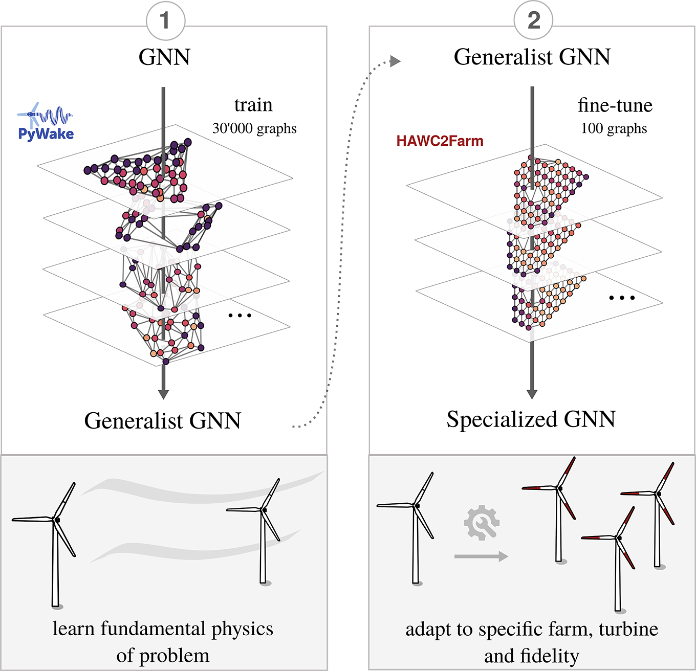
As stated in the introductory section, this contribution attempts to develop a flexible method for multivariate prediction on wind farms. Specifically, we attempt to estimate the fatigue and aerodynamic loads for random inflow conditions, given a wind farm layout that is unseen during model training, or in other words not used in the training set. We build upon the methodology described in Duthàet al. (Reference Duthé, de N Santos, Abdallah, Réthoré, Weijtjens, Chatzi and Devriendt2023b) and in de N Santos et al. (Reference de N Santos, Duthé, Abdallah, Réthoré, Weijtjens, Chatzi and Devriendt2024a), wherein PyWake aeroelastic simulations are used to train and validate GNNs. In this work, we rely on the speed of PyWake to easily generate load estimations for a wide range of inflow conditions and farm layouts. These are used to train a ’generalist’ GNN, i.e. a baseline GNN capable of understanding the fundamental physics of the problem. After the training of the generalist GNN we fine-tune it for a specific farm and turbine configuration (Lillgrund), given a limited dataset of higher-fidelity simulations modelled with HAWC2Farm. In this contribution, in particular, we compare three fine-tuning techniques: full model tuning, decoder-only tuning and LoRA. An overview of our approach can be observed in Figure 1.
Methodological overview. We first train a generalist GNN on a large dataset of random PyWake simulation graphs, giving it an understanding of the underlying physics. Then, we fine-tune the model for a specific wind farm with a small dataset of higher-fidelity HAWC2Farm simulations.
3. Related work
3.1. Current modelling of wind farms
The operation, layout optimization and control of modern wind farms remain open areas of study as load estimation under real conditions is still difficult. This difficulty lies fundamentally with the complex interactions between wind farms and the highly turbulent, non-stationary and often heterogeneous atmospheric boundary layer, along with the intra-farm turbulent wake flows (Porté-Agel et al., Reference Porté-Agel, Bastankhah and Shamsoddin2020). A further complexity stems from the fact that wind farms are affected by wide-ranging flow conditions and turbulent scales, from the weather meso- and macroscale to the atmospheric boundary layer integral scale and Kolmogorov microscale (Veers et al., Reference Veers2019). It is the multi-scale nature of the bidirectional influence between turbines and flow that increases the problem’s complexity.
There exist various approaches for modelling the interaction of wind turbine and wind farm with flow. Apart from experimental approaches (which we will not approach in this contribution), so-called ’engineering’ or analytical methods, and CFD can be used. The first class predicts wake deficits by applying basic physical equations that govern the conservation of flow properties (e.g., mass, momentum and energy) for different regions (near- and far-wake) (Porté-Agel et al., Reference Porté-Agel, Bastankhah and Shamsoddin2020). The flow solver PyWake implements a series of these methods, which are relatively fast. However, these methods are necessarily less accurate than numerical models due to their simplifications. This is particularly troublesome for fatigue load estimation, as these depend on a three-dimensional description of the flow field.
Numeric/CFD models, on the other hand, like Reynolds-Aeraged Navier-Stokes (RANS) and LES, give more accurate descriptions of wind farm flow fields, but they are still too computationally expensive for industry employment, although advances made, particularly for LES, might yet open the door to near real-time LES-based control (Janssens and Meyers, Reference Janssens and Meyers2023). Therefore, aeroelastic simulations at the farm level necessarily represent a trade-off between precise load prediction and computational cost (Liew et al., Reference Liew, Andersen, Troldborg and Göçmen2022). Thus, a clear gap exists between fast and coarse, and slow and fine simulations. This has led to use of surrogate modeling techniques, frequently implemented through machine learning algorithms (Simpson et al., Reference Simpson, Dervilis and Chatzi2021; Mylonas et al., Reference Mylonas, Abdallah and Chatzi2021a), for estimating wind farm dynamic responses. The present contribution inserts itself in this constellation, where we attempt to employ machine learning techniques (GNNs) for surrogate modelling of flow solvers. We specifically attempt to bridge the gap between different fidelity-level solvers (PyWake and HAWC2Farm) through multi-fidelity transfer learning.
3.2. GNNs and their applications for physics-based problems
Graph-based deep learning (Battaglia et al., Reference Battaglia2018), which is a subset of geometric deep learning (Bronstein et al., Reference Bronstein, Bruna, LeCun, Szlam and Vandergheynst2017), is a type of machine learning that is non-Euclidean, meaning that is not restricted to fixed-size inputs and outputs. It is increasingly being explored for its potential in addressing a variety of problems in physics, as indicated by research in Sanchez-Gonzalez et al. (Reference Sanchez-Gonzalez, Heess, Springenberg, Merel, Riedmiller, Hadsell and Battaglia2018) and expanded upon in Sanchez-Gonzalez et al. (Reference Sanchez-Gonzalez, Godwin, Pfaff, Ying, Leskovec and Battaglia2020). This growing adoption can be attributed to its powerful representational capabilities. Although the development of learning on graphs has been relatively slower due to challenges arising from graph-encoded data, such as differentiability issues caused by graph discreteness or loops, recent years have witnessed significant progress in deep learning on graphs. Building upon foundational works (Scarselli et al., Reference Scarselli, Gori, Tsoi, Hagenbuchner and Monfardini2008; Micheli, Reference Micheli2009), these advancements have propelled graph-based deep learning to the forefront. As a result, graph-based methods have become integral to the machine learning community, with algorithms developed for deep learning on graphs finding widespread adoption across various domains. For instance, Pfaff et al. (Reference Pfaff, Fortunato, Sanchez-Gonzalez and Battaglia2020) provide an example of GNNs being employed to emulate the operations of conventional mesh-based physics simulators, with an ability to forecast the progression of transient solutions. Our methodology also adopts the Encode-Process-Decode pipeline introduced in the aforementioned works, as it is has proven to be effective at learning underlying physical processes in multiple different domains. One such domain, is the reconstruction of flows around airfoils in high Reynolds turbulent inflow conditions (Duthé et al., Reference Duthé, Abdallah, Barber and Chatzi2023a). This setup has also seen success when combined with physics-informed objective functions (Hernández et al., Reference Hernández, Badías, Chinesta and Cueto2022). Moreover, GNNs have proven to be adept at approximating the solutions to PDEs (Li et al., Reference Li, Kovachki, Azizzadenesheli, Liu, Bhattacharya, Stuart and Anandkumar2020b) and even performing medium-range weather forecasting at a level that is on par or superior to the currently-used computational methods (Lam et al., Reference Lam2023).
3.3. GNNs for wind farms
Despite still being a nascent subfield of machine learning, GNNs have attracted a significant amount of attention in the domain of wind energy applications, with their usage primarily concentrated on power (Bentsen et al., Reference Bentsen, Warakagoda, Stenbro and Engelstad2022; Yu et al., Reference Yu2020; Park and Park, Reference Park and Park2019) and wake loss predictions (Bleeg, Reference Bleeg2020; Li et al., Reference Li, Zhang and Piggott2022; Levick et al., Reference Levick, Neubert, Friggo, Downes, Ruisi and Bleeg2022). Bentsen et al. (Reference Bentsen, Warakagoda, Stenbro and Engelstad2022) employ graph attention networks (GAT, Veličković et al. (Reference Veličković, Cucurull, Casanova, Romero, Lio and Bengio2017)) to predict the expected power production on a farm. The attention mechanism offers insights into the model’s learning, with it seemingly capturing turbine dependencies that are aligned with physical intuition on wake losses. Similarly, Yu et al. (Reference Yu2020) utilize a so-called Superposition Graph Neural Network, where a temporal superposition of spatial graphs is used to predict the generated power of four different wind farms. Park and Park (Reference Park and Park2019) employ a physics-informed GNN (PGNN, introducing the physics through a engineering wake interaction model as a basis function) to estimate the power outputs of all wind turbines in any layout under any wind conditions. Bleeg (Reference Bleeg2020), on the other hand, attempts to estimate the turbine interaction loss, taking into account both wake and blockage effects using a generic GNN. They show that their proposed model combines the speed of wake models with precision that is comparable to a high-fidelity RANS flow model. Similarly, based on RANS wake data generated using a generalised actuator disk (GAD) model coupled with the CFD solver package OpenFOAM, Li et al. (Reference Li, Zhang and Piggott2022) utilize GraphSAGE (Graph SAmple and aggreGatE, Hamilton et al. (Reference Hamilton, Ying and Leskovec2017)) for flow field reconstruction. This graph deep learning surrogate model was able to simulate wind farms within seconds, in comparison to several hours of parallel computing usually needed for a RANS simulation. Finally, Mylonas et al. (Reference Mylonas, Abdallah and Chatzi2021b) combine GNNs with Variational Bayes in a so-called Relational Variational Autoencoder (RVAE) approach to estimate farm-wide wind deficits and compare with simulated results using a steady-state wind farm wake simulator.
3.4. Approaches to transfer learning and fine-tuning
Transfer learning has become an important part of machine learning research, driven by the need for versatile frameworks which can leverage knowledge from one domain to improve performance in another (Tan et al., Reference Tan, Sun, Kong, Zhang, Yang and Liu2018). Transfer learning refers to methodologies which, in general, aim to leverage learned low-level features from a source domain in order improve performance in a target domain which is often much sparser. Popular methods for transfer learning in which the source and target distributions are different include Transfer Component Analysis (Pan et al., Reference Pan, Tsang, Kwok and Yang2010) and Joint Distribution Adaptation (Long et al., Reference Long, Wang, Ding, Sun and Yu2013). When the source and target domains are very similar, or when the target domain is a more detailed subset of the source domain, one may think of transfer learning in terms of fine-tuning. With fine-tuning, the aim is to retain most of the learned behavior and only adjust certain parts of the model. This is the case for our problem, where we first aim to learn the underlying physics with lower-fidelity data, and then fine-tune on specific configurations using higher-fidelity data. This pretrain-then-finetune paradigm has recently become a popular configuration with the advent of generalist Large Language Models (LLMs) that are costly to retrain (Radford et al., Reference Radford, Narasimhan, Salimans and Sutskever2018; Brown et al., Reference Brown2020). It allows developers to leverage powerful models for niche tasks which were previously too specific to justify the costs associated with training such powerful models. Usually, fine-tuning updates all the learnable parameters of a model (Dodge et al., Reference Dodge, Ilharco, Schwartz, Farhadi, Hajishirzi and Smith2020), or sometimes certain specific layers (Guo et al., Reference Guo, Shi, Kumar, Grauman, Rosing and Feris2019). However, the increase in fine-tuning efficiency is an active field of research with several popular techniques having recently emerged (Ding et al., Reference Ding2023). One such method, which we experiment with in the present work and which we detail later, is Low Rank Adaptation (LoRA) (Hu et al., Reference Hu2021).
Transfer learning is especially interesting in the context of population-based SHM (PBSHM) (Worden et al., Reference Worden2020; Hughes et al., Reference Hughes, Poole, Dervilis, Gardner and Worden2023), allowing higher-level monitoring of structures by utilizing existing data from a source structure to improve knowledge about a target structure, for which data is sparse. GNNs in particular have shown promise for transfer learning in PBSHM, enabling researchers to efficiently extrapolate properties across populations of structures such as trusses (Tsialiamanis et al., Reference Tsialiamanis, Mylonas, Chatzi, Wagg, Dervilis and Worden2022). For wind energy, several studies which apply transfer learning exist, where these often involve adapting a model trained on a specific wind farm for use on a different farm (Zgraggen et al., Reference Zgraggen, Ulmer, Jarlskog, Pizza and Huber2021; Yin et al., Reference Yin, Ou, Fu, Cai, Chen and Meng2021). Finally, with respect to PBSHM of individual turbines, Black et al. (Reference Black, Cevasco and Kolios2022) applied a neural network, trained on measured gearbox data from one turbine, to monitor the health of a different turbine within the same farm.
4. Data
4.1. Low fidelity simulations via PyWake
4.1.1. Random wind farm layout generation
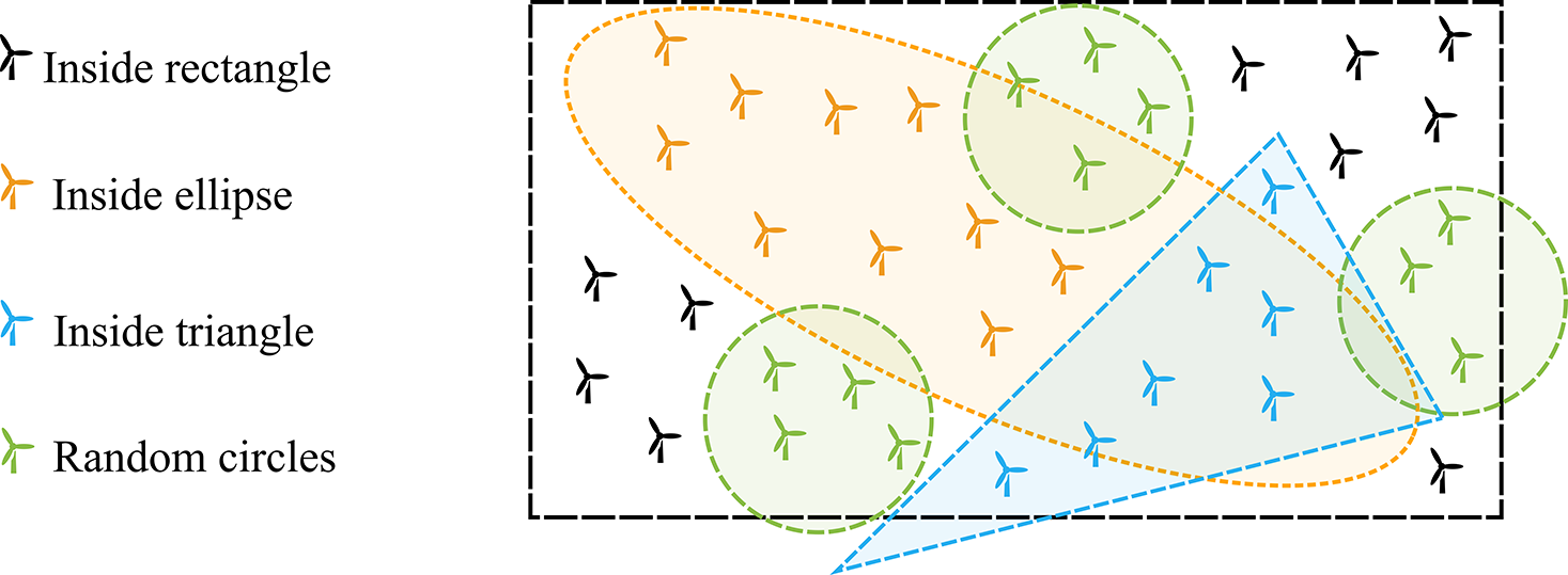
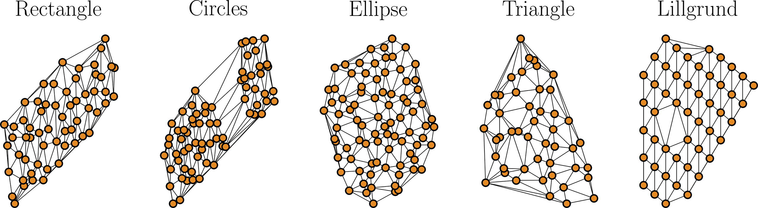
To produce a robust pre-training dataset, with many different arbitrary layout geometries, we first need to construct an arbitrary wind farm layout generation methodology. We create layout geometries for wind farms using a random sampling method with four basic geometries: rectangles, triangles, ellipses, and sparse circles. To do so, we first select a minimum distance between turbines, which depends on the rotor diameter (c.f. Table 3). Then, a set of initial points for each random base geometry is generated, equally spaced and then randomly perturbed and rotated by a random angle, using O’Neill’s permutation congruential generator (PCG, (O’Neill, Reference O’Neill2014), as implemented by numpy.random). An example of the random layout geometry generation is shown in Figure 2 for a set of wind turbines, with the four geometrical shapes superimposed. To produce a unique layout, only one of the four defined geometries is chosen for each training sample set, though the resulting layout is arbitrary.
Illustration of random generation of wind farm layouts through pooling points inside different basic geometries (rectangle, triangle, ellipse, and sparse circles), randomly perturbed and rotated.
4.1.2. Sampling inflow conditions
To conduct farm-wide aerodynamic simulations using PyWake, one must specify the far-field turbulent inflow wind conditions. These conditions are characterized by several random variables, namely the mean wind speed (
 $ u $
), turbulence intensity (
$ u $
), turbulence intensity (
 $ {T}_i $
), wind shear (
$ {T}_i $
), wind shear (
 $ \alpha $
), and horizontal inflow skewness (
$ \alpha $
), and horizontal inflow skewness (
 $ \Psi $
) (Avendaño-Valencia et al., Reference Avendaño-Valencia, Abdallah and Chatzi2021). The mean wind speed is modeled using a truncated Weibull distribution, defined by its scale and shape parameters, respectively, as:
$ \Psi $
) (Avendaño-Valencia et al., Reference Avendaño-Valencia, Abdallah and Chatzi2021). The mean wind speed is modeled using a truncated Weibull distribution, defined by its scale and shape parameters, respectively, as:
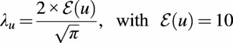 $$ {\lambda}_u=\frac{2\times \mathcal{E}(u)}{\sqrt{\pi }},\hskip1em \mathrm{with}\hskip1em \mathcal{E}(u)=10 $$
 $$ {k}_u=2.0. $$
The wind turbine design standard (Commission et al., Reference Commission2005) describes a Normal Turbulence Model which defines the conditional dependence between the turbulence,
 $ {\sigma}_u $
and the mean wind speed,
$ {\sigma}_u $
and the mean wind speed,
 $ u $
. The elected reference ambient turbulence intensity (its expected value at 15
$ u $
. The elected reference ambient turbulence intensity (its expected value at 15
 $ \mathrm{m}.{\mathrm{s}}^{-1} $
) was
$ \mathrm{m}.{\mathrm{s}}^{-1} $
) was
 $ {I}_{ref}=0.16 $
. This dependency is given by the local statistical moments of the log-normal distribution (Johnson et al., Reference Johnson, Kotz and Balakrishnan1995), given by
$ {I}_{ref}=0.16 $
. This dependency is given by the local statistical moments of the log-normal distribution (Johnson et al., Reference Johnson, Kotz and Balakrishnan1995), given by
 $ {\sigma}_u\sim \mathrm{\mathcal{L}}\mathcal{N}\left({\mu}_{\sigma_u},{\sigma}_{\sigma_u}^2\right) $
, with:
$ {\sigma}_u\sim \mathrm{\mathcal{L}}\mathcal{N}\left({\mu}_{\sigma_u},{\sigma}_{\sigma_u}^2\right) $
, with:
 $$ \unicode{x1D53C}\left({\sigma}_u|u\right)={I}_{ref}\cdot \left(0.75u+3.8\right) $$
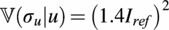 $$ \unicode{x1D54D}\left({\sigma}_u|u\right)={\left(1.4{I}_{ref}\right)}^2 $$
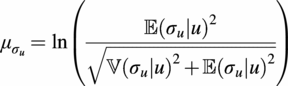 $$ {\mu}_{\sigma_u}=\ln \left(\frac{\unicode{x1D53C}{\left({\sigma}_u|u\right)}^2}{\sqrt{\unicode{x1D54D}{\left({\sigma}_u|u\right)}^2+\unicode{x1D53C}{\left({\sigma}_u|u\right)}^2}}\right) $$
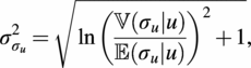 $$ {\sigma}_{\sigma_u}^2=\sqrt{\ln {\left(\frac{\unicode{x1D54D}\left({\sigma}_u|u\right)}{\unicode{x1D53C}\left({\sigma}_u|u\right)}\right)}^2+1}, $$
and we define the turbulence intensity as
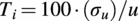 $ {T}_i=100\cdot \left({\sigma}_u\right)/u $
. As for the wind profile above ground level, this is described by a power law relationship that is adopted to express the mean wind speed
$ {T}_i=100\cdot \left({\sigma}_u\right)/u $
. As for the wind profile above ground level, this is described by a power law relationship that is adopted to express the mean wind speed
 $ u $
at height
$ u $
at height
 $ Z $
above ground as a function of the mean wind speed at hub height
$ Z $
above ground as a function of the mean wind speed at hub height
 $ {u}_h $
, measured at hub height
$ {u}_h $
, measured at hub height
 $ {Z}_h $
:
$ {Z}_h $
:
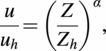 $$ \frac{u}{u_h}={\left(\frac{Z}{Z_h}\right)}^{\alpha }, $$
where
 $ \alpha $
is the shear exponent, of constant value. We sample the wind shear exponent from a truncated normal distribution (Casella and Berger, Reference Casella and Berger2021),
$ \alpha $
is the shear exponent, of constant value. We sample the wind shear exponent from a truncated normal distribution (Casella and Berger, Reference Casella and Berger2021),
 $ \alpha \sim \mathcal{N}\left({\mu}_{\alpha },{\sigma}_{\alpha}^2\right) $
with bounds
$ \alpha \sim \mathcal{N}\left({\mu}_{\alpha },{\sigma}_{\alpha}^2\right) $
with bounds
 $ \left[-\mathrm{0.099707,0.499414}\right] $
.
$ \left[-\mathrm{0.099707,0.499414}\right] $
.
The conditional dependence between the wind shear exponent,
 $ \alpha $
, and the mean wind speed,
$ \alpha $
, and the mean wind speed,
 $ u $
, is given by Dimitrov et al. (Reference Dimitrov, Natarajan and Kelly2015):
$ u $
, is given by Dimitrov et al. (Reference Dimitrov, Natarajan and Kelly2015):
 $$ \unicode{x1D53C}\left(\alpha |u\right)=0.088\cdot \left(\log (u)-1\right) $$
 $$ \unicode{x1D54D}\left(\alpha |u\right)={\left(\frac{1}{u}\right)}^2. $$
Additionally, a custom conditional dependence between the inflow horizontal skewness,
 $ \Psi $
, and the mean wind speed,
$ \Psi $
, and the mean wind speed,
 $ u $
, is defined by the truncated normal distribution
$ u $
, is defined by the truncated normal distribution
 $ \Psi \sim \mathcal{N}\left({\mu}_{\Psi},{\sigma}_{\Psi}^2\right) $
, with bounds
$ \Psi \sim \mathcal{N}\left({\mu}_{\Psi},{\sigma}_{\Psi}^2\right) $
, with bounds
 $ \left[-6,6\right]{}^{\circ} $
:
$ \left[-6,6\right]{}^{\circ} $
:
 $$ \unicode{x1D53C}\left(\Psi |u\right)=\ln (u)-3 $$
 $$ \unicode{x1D54D}\left(\Psi |u\right)={\left(\frac{15}{u}\right)}^2. $$
Finally, the wind direction was sampled from a uniform distribution (Dekking et al., Reference Dekking, Kraaikamp, Lopuhaä and Meester2005),
 $ \Omega \sim {\mathcal{U}}_{\left[\mathrm{0,360}\right]} $
, spanning the full
$ \Omega \sim {\mathcal{U}}_{\left[\mathrm{0,360}\right]} $
, spanning the full
 $ \left[\mathrm{0,360}\right]{}^{\circ} $
interval. The full settings used for the inflow variables generation can be found in Table 1.
$ \left[\mathrm{0,360}\right]{}^{\circ} $
interval. The full settings used for the inflow variables generation can be found in Table 1.
Wind farm freestream inflow random variables
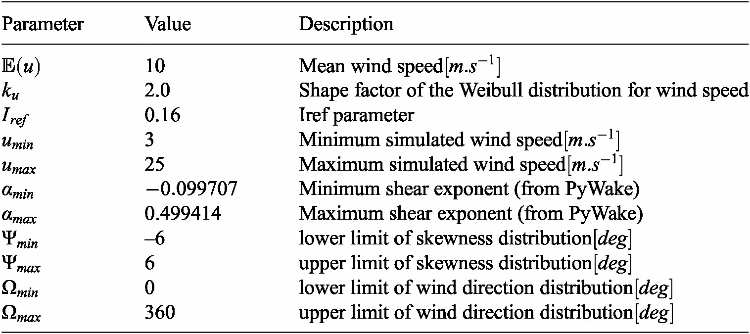
We choose to sample the turbulent inflow wind field variables (
 $ u $
,
$ u $
,
 $ {T}_i $
,
$ {T}_i $
,
 $ \alpha $
,
$ \alpha $
,
 $ \Psi $
and
$ \Psi $
and
 $ \Omega $
) through Sobol Quasi-Random sequences (Sobol, Reference Sobol’1967), of
$ \Omega $
) through Sobol Quasi-Random sequences (Sobol, Reference Sobol’1967), of
 $ n={2}^m $
low discrepancy points in
$ n={2}^m $
low discrepancy points in
 $ {\left[0,1\right]}^d $
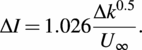
. These generate uniformly distributed samples over the multi-dimensional input space (unit hypercube, Saltelli et al. (Reference Saltelli, Annoni, Azzini, Campolongo, Ratto and Tarantola2010)). In Figure 3, we can observe the matrix plot of dependence between each inflow variable’s samples.
$ {\left[0,1\right]}^d $
. These generate uniformly distributed samples over the multi-dimensional input space (unit hypercube, Saltelli et al. (Reference Saltelli, Annoni, Azzini, Campolongo, Ratto and Tarantola2010)). In Figure 3, we can observe the matrix plot of dependence between each inflow variable’s samples.
Samples from the joint wind inflow random variables. Non-diagonal plots additionally present a 4-level bivariate distribution through a Gaussian kernel density estimate (KDE) (Chen, Reference Chen2017).
4.1.3. PyWake simulator setup
The simulations used for GNN pre-training are generated using PyWake (Pedersen et al., Reference Pedersen, van der Laan, Friis-Møller, Rinker and Réthoré2019), a multi-fidelity wind farm flow simulation tool. Utilizing Python and the numpy package, PyWake offers an interface to various engineering models, and is particularly efficient at analyzing wake propagation and turbine interactions within a wind farm or even farm-to-farm (Fischereit et al., Reference Fischereit, Schaldemose Hansen, Larsén, van der Laan, Réthoré and Murcia Leon2022). Its goal is to provide a cost-effective way to calculate wake interactions under various steady state conditions, and it can be used to estimate power production while accounting for wake losses in a particular wind farm layout. This makes it particularly well-suited for the quick generation of a large farm-wide dataset, albeit at reduced precision than, for instance, aeroelastic wind farm simulators. We use PyWake to produce our base dataset, with thousands of random farm layouts and inflow configurations.
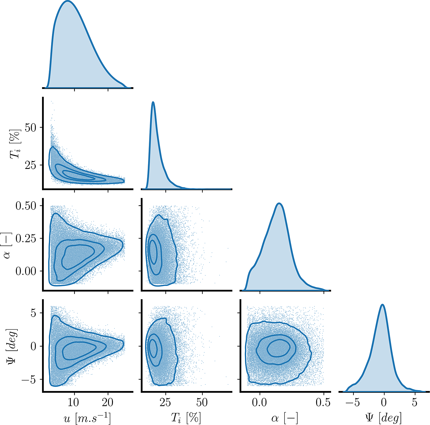
Due to its modularity, PyWake allows the use of a number of engineering models. In this particular application, we adopt Niayifar’s Gaussian wake deficit model (Niayifar and Porté-Agel, Reference Niayifar and Porté-Agel2016). Niayifar proposes a wake expansion/growth rate
 $ k $
that varies linearly with local turbulence intensity:
$ k $
that varies linearly with local turbulence intensity:
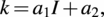 $$ k={a}_1I+{a}_2, $$
with I, the local streamwise turbulence intensity immediately upwind of the rotor center, estimated neglecting blockage effects, and the coefficients
 $ {a}_1=0.3837 $
and
$ {a}_1=0.3837 $
and
 $ a2=0.0036 $
based on Large-Eddy Simulations (LES) of Bastankhah and Porté-Agel (Reference Bastankhah and Porté-Agel2014).
$ a2=0.0036 $
based on Large-Eddy Simulations (LES) of Bastankhah and Porté-Agel (Reference Bastankhah and Porté-Agel2014).
The interaction among multiple wakes is modeled based on the velocity deficit superposition principle, with the velocity deficit calculated as the difference between the inflow velocity at the turbine and the wake velocity:
 $$ {U}_i={U}_{\infty }-\sum \limits_{k=1}^n\left({U}_k-{U}_{ki}\right). $$
Regarding the turbulence intensity model, we employ the Crespo-Hernández’s model (Crespo and Hernández, Reference Crespo and Hernández1996), where the added turbulence intensity is given by:
 $$ \Delta I=1.026\frac{\Delta {k}^{0.5}}{U_{\infty }}. $$
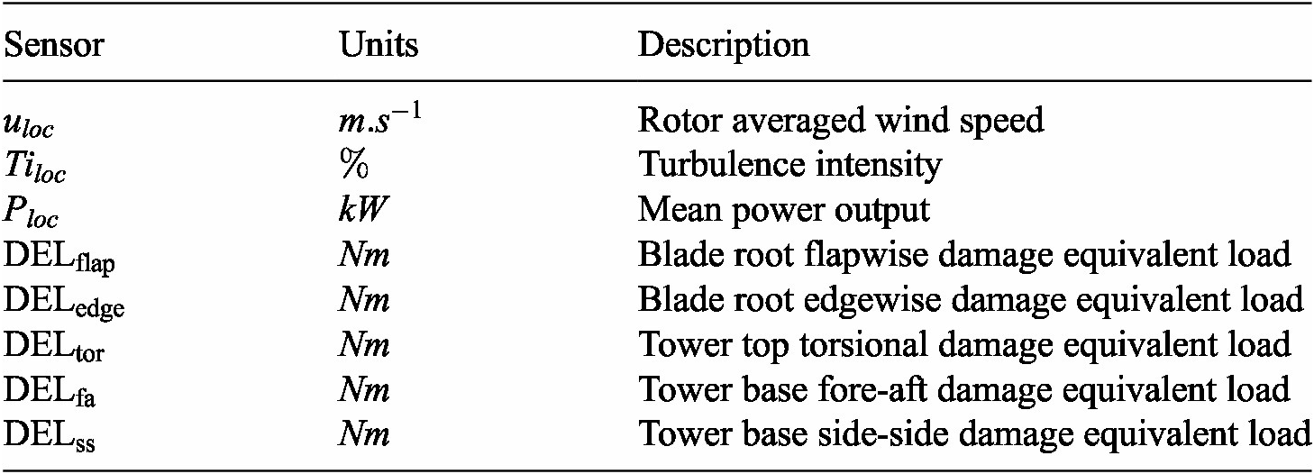
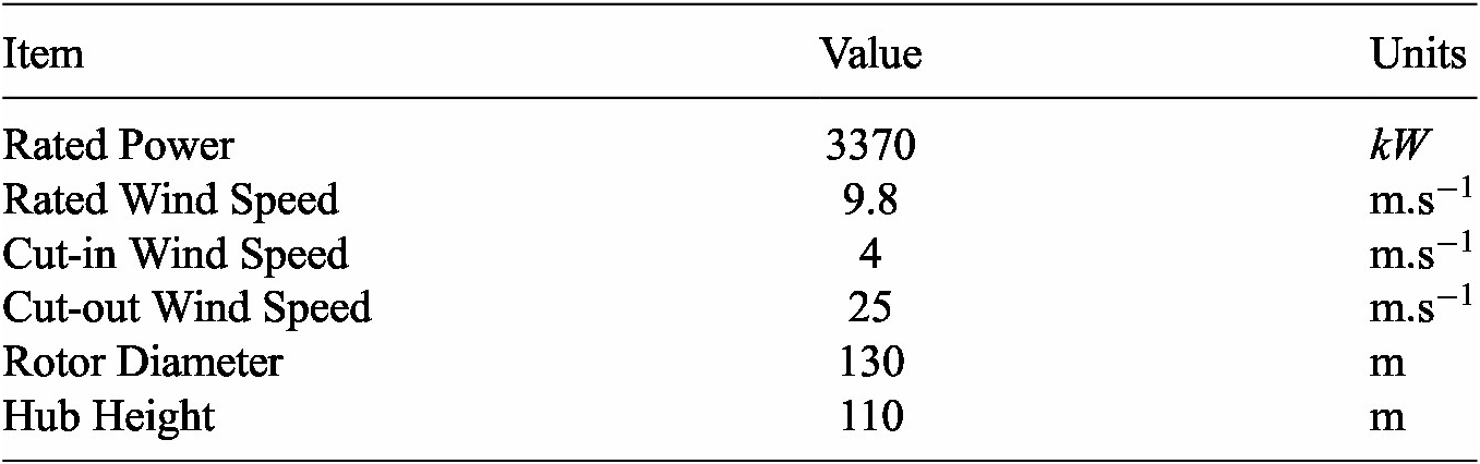
As for the fatigue load estimation, PyWake implements in its two wind-turbine approach a neural network surrogate of HAWC2 simulations (Larsen and Hansen, Reference Larsen and Hansen2007) in different wake and inflow conditions, where the wind farm is split into pairs of wind turbines and returns the load of the pair that yields the highest load. PyWake can report for each turbine in a simulated farm 8 ’sensor’ quantities which we describe in Table 2. In our analysis, we use the International Energy Agency’s (IEA) 3.4
 $ MW $
reference wind turbine (RWT, Bortolotti et al. (Reference Bortolotti, Tarres, Dykes, Merz, Sethuraman, Verelst and Zahle2019)), as described in Table 3.
$ MW $
reference wind turbine (RWT, Bortolotti et al. (Reference Bortolotti, Tarres, Dykes, Merz, Sethuraman, Verelst and Zahle2019)), as described in Table 3.
PyWake outputed quantities
Characteristics of the IEA 3.4
 $ MW $
reference wind turbine used in PyWake
$ MW $
reference wind turbine used in PyWake
Utilizing the described pipeline, we synthesize a dataset of 3,000 randomly selected wind farm layouts, with each layout being subjected to a unique set of 10 different random inflow conditions. Consequently, this process yields a total of 30,000 unique graphs that can be used to pre-train our GNN model. The full dataset can be found in de N Santos et al. (Reference de N Santos, Duthé, Abdallah, Réthoré, Weijtjens, Chatzi and Devriendt2023a).
4.2. High fidelity aeroelastic simulations
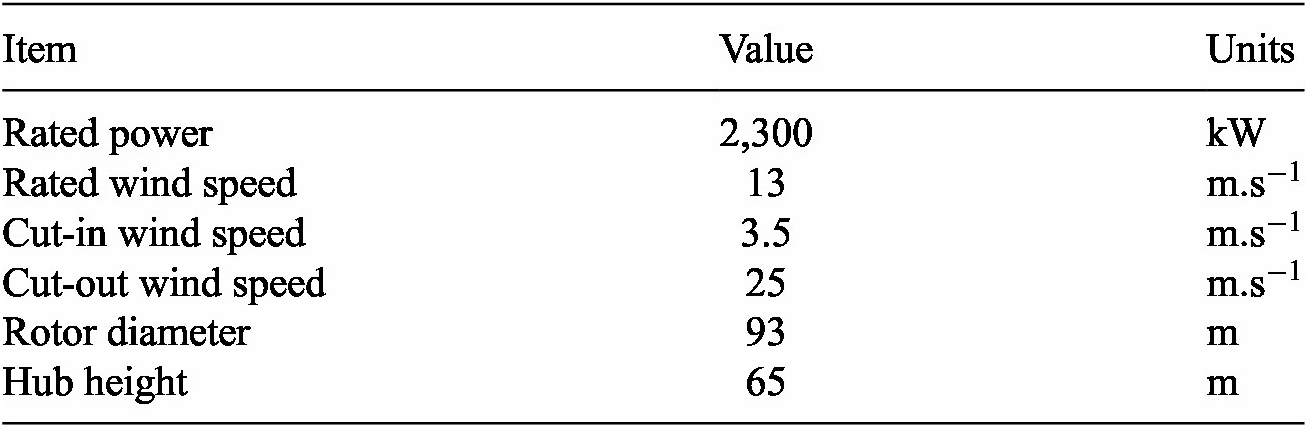
To develop and test our multi-fidelity transfer framework, we make use of a dataset of aeroelastic simulations generated by Liew et al. (Reference Liew, Riva and Göçmen2023a). The authors present a comprehensive database of 1000 one-hour long simulations of the Lillgrund offshore wind farm computed using HAWC2Farm. This farm is composed of 48 2.3
 $ MW $
Siemens SWT-2.3-93 turbines, the characteristics of which can be found in Table 4. HAWC2Farm models each individual turbine of a wind farm using the HAWC2 aeroelastic simulator (Larsen and Hansen, Reference Larsen and Hansen2007), with their interactions being computed using a dynamic wake meandering model (Larsen et al., Reference Larsen, Madsen, Thomsen and Larsen2008). Here, the simulations are performed at a sampling rate of 100 Hz using a large turbulence box which covers the entire farm. In the box, turbulence is generated using the presented Mann turbulence model implementation. The authors use the Halton sequence (Halton, Reference Halton1960) to sample a range of ambient wind speeds from 4 m/s to 20 m/s, turbulence intensities from 2.5%to 10%, wind directions from 0 to 360 degrees, and shear exponents ranging from 0 to 0.3. The dataset, thus, captures the dynamic structural response and fatigue loading of the 48 turbines in the farm across a reasonably wide range of operating conditions.
$ MW $
Siemens SWT-2.3-93 turbines, the characteristics of which can be found in Table 4. HAWC2Farm models each individual turbine of a wind farm using the HAWC2 aeroelastic simulator (Larsen and Hansen, Reference Larsen and Hansen2007), with their interactions being computed using a dynamic wake meandering model (Larsen et al., Reference Larsen, Madsen, Thomsen and Larsen2008). Here, the simulations are performed at a sampling rate of 100 Hz using a large turbulence box which covers the entire farm. In the box, turbulence is generated using the presented Mann turbulence model implementation. The authors use the Halton sequence (Halton, Reference Halton1960) to sample a range of ambient wind speeds from 4 m/s to 20 m/s, turbulence intensities from 2.5%to 10%, wind directions from 0 to 360 degrees, and shear exponents ranging from 0 to 0.3. The dataset, thus, captures the dynamic structural response and fatigue loading of the 48 turbines in the farm across a reasonably wide range of operating conditions.
Characteristics of the Siemens SWT-2.3-93 wind turbines of the Lillgrund wind farm
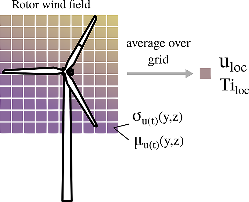
For our testing, we use a subset of 800 of these simulations which was made publicly available (Liew et al., Reference Liew, Riva and Göçmen2023b). In this dataset, the local flow conditions are parameterized by a 30x30 grid in front of each turbine rotor, where each cell of this grid contains the average and the standard deviation of the flow gathered over 10 minutes. To obtain comparable local flow outputs to PyWake, we therefore first have to convert the velocity grids. Taking the mean of the time-averaged velocity over this grid gives an estimation of the local value of the wind speed, while the local turbulence intensity can be computed by dividing the mean velocity by the mean over the grid of the time-gathered standard deviation of each cell. Figure 4 illustrates this process. The remaining variables that we require can be directly extracted from the 10-minute average HAWC2 outputs included in the dataset. The initial HAWC2 simulations have a duration of 1 hour each, yielding six 10 minute periods of averaged quantities for each variable and each simulation. We only keep the first such period of each simulation, as the difference in the resulting averaged variables between these periods is minimal.
Illustration of inference of local flow quantities from the vertical grid in front of each turbine for the HAWC2Farm dataset.
4.2.1. Visualizing wake effects and model disparities
In Figure 5 we plot, for the Lillgrund wind farm layout and a predominant wind direction N–NE (
 $ \Omega $
), the HAWC2Farm and PyWake outputs for two turbines under different flow conditions: WT 31 (blue, free-flow), WT 35 (orange, wake-affected). In this figure, we observe how the wake-affected turbine, which is located in the middle of the farm under strong wake conditions, present much higher damage-equivalent loads, more evident for fore-aft, torsional and flapwise DELs, which makes physical sense. There are large differences in the magnitude of the DELs, with HAWC2 loads being dwarfed by those from the PyWake simulations. This occurs due to the different turbine models used in each simulator. Despite these differences, the underlying physics are similar, as highlighted by the behavior of the local turbulence intensity, wind speed and power.
$ \Omega $
), the HAWC2Farm and PyWake outputs for two turbines under different flow conditions: WT 31 (blue, free-flow), WT 35 (orange, wake-affected). In this figure, we observe how the wake-affected turbine, which is located in the middle of the farm under strong wake conditions, present much higher damage-equivalent loads, more evident for fore-aft, torsional and flapwise DELs, which makes physical sense. There are large differences in the magnitude of the DELs, with HAWC2 loads being dwarfed by those from the PyWake simulations. This occurs due to the different turbine models used in each simulator. Despite these differences, the underlying physics are similar, as highlighted by the behavior of the local turbulence intensity, wind speed and power.
PyWake and HAWC2Farm outputted quantities vs. global far-field wind speed for two wind turbines of the Lillgrund layout under contrasting wake conditions, for a range of N-E inflows. The simulated turbines are different for the two simulators, yielding vastly different loads. Shaded curves represent the 75% and 95% distribution percentiles.

Aside quantitative differences, there are, however, qualitative differences which exemplify the lower ability of PyWake, namely the offsets present for the blade fatigue loads (edge- and flapwise), along with serious jumps, as seen for fore-aft and side-to-side. The observed differences stem from the different levels of simulation fidelity between PyWake and HAWC2. While PyWake employs engineering wake-expansion models coupled with a machine learning-based surrogate for aeroelastic load estimation, HAWC2 is a comprehensive aeroelastic code that conducts time-domain simulations to capture a wind turbine’s dynamic response. Thus, the loads computed via HAWC2Farm are inherently more nuanced than those given by PyWake.
5. Graph neural network framework
5.1. Establishing the graphs
A wind farm can be modeled as a graph
 $ \mathcal{G}=\left(\mathcal{V},\mathrm{\mathcal{E}},\mathbf{X},\mathbf{E},\mathbf{W}\right) $
, where
$ \mathcal{G}=\left(\mathcal{V},\mathrm{\mathcal{E}},\mathbf{X},\mathbf{E},\mathbf{W}\right) $
, where
 $ \mathcal{V} $
represents a set of
$ \mathcal{V} $
represents a set of
 $ n $
nodes (individual turbines), and
$ n $
nodes (individual turbines), and
 $ \mathrm{\mathcal{E}} $
is the set of
$ \mathrm{\mathcal{E}} $
is the set of
 $ k $
edges which represent the interactions between turbines. Each turbine node
$ k $
edges which represent the interactions between turbines. Each turbine node
 $ i $
is associated with a feature vector
$ i $
is associated with a feature vector
 $ {\mathbf{x}}_i\in \mathbf{X} $
, containing
$ {\mathbf{x}}_i\in \mathbf{X} $
, containing
 $ {f}_n $
physical measurements and/or properties (e.g., power, loads, local effective turbulence intensity). For each edge connecting turbines
$ {f}_n $
physical measurements and/or properties (e.g., power, loads, local effective turbulence intensity). For each edge connecting turbines
 $ i $
and
$ i $
and
 $ j $
, an attribute vector
$ j $
, an attribute vector
 $ {\mathbf{e}}_{i,j}\in \mathbf{E} $
is defined, encapsulating the
$ {\mathbf{e}}_{i,j}\in \mathbf{E} $
is defined, encapsulating the
 $ {f}_e $
geometrical properties of the edge. The wind farm graph also includes a global property vector
$ {f}_e $
geometrical properties of the edge. The wind farm graph also includes a global property vector
 $ \mathbf{W}\in {\mathrm{\mathbb{R}}}^{f_g} $
, of size 3, to represent farm-level inflow conditions.
$ \mathbf{W}\in {\mathrm{\mathbb{R}}}^{f_g} $
, of size 3, to represent farm-level inflow conditions.
 $ \mathbf{X}\in {\mathrm{\mathbb{R}}}^{n\times {f}_n} $
, and
$ \mathbf{X}\in {\mathrm{\mathbb{R}}}^{n\times {f}_n} $
, and
 $ \mathbf{E}\in {\mathrm{\mathbb{R}}}^{k\times {f}_e} $
are respectively the node and edge feature matrices of this graph representation. This section details how the edge connectivity is constructed and describes the input and output attributes of the graphs.
$ \mathbf{E}\in {\mathrm{\mathbb{R}}}^{k\times {f}_e} $
are respectively the node and edge feature matrices of this graph representation. This section details how the edge connectivity is constructed and describes the input and output attributes of the graphs.
5.1.1. Graph connectivity
Various methods could be used to determine the graph edge connectivity
 $ \mathrm{\mathcal{E}} $
for a specific wind farm layout. In this work, we choose to employ a widely-used meshing technique for the generation of unstructured triangular meshes, the Delaunay triangulation (Delaunay et al., Reference Delaunay1934; Musin, Reference Musin1997). Unlike other popular point-to-graph generation techniques (radial, k-nearest-neighbours), this method ensures that no isolated communities are formed, i.e. that the generated graph is connected. Moreover, previous results (Duthé et al., Reference Duthé, de N Santos, Abdallah, Réthoré, Weijtjens, Chatzi and Devriendt2023b) have shown that against the fully-connected method, in which all vertices of a graph are connected to each-other, Delaunay triangulation yields comparable results at a much lesser computational cost. We show in Figure 6 some examples of wind farm graphs connected using this method.
$ \mathrm{\mathcal{E}} $
for a specific wind farm layout. In this work, we choose to employ a widely-used meshing technique for the generation of unstructured triangular meshes, the Delaunay triangulation (Delaunay et al., Reference Delaunay1934; Musin, Reference Musin1997). Unlike other popular point-to-graph generation techniques (radial, k-nearest-neighbours), this method ensures that no isolated communities are formed, i.e. that the generated graph is connected. Moreover, previous results (Duthé et al., Reference Duthé, de N Santos, Abdallah, Réthoré, Weijtjens, Chatzi and Devriendt2023b) have shown that against the fully-connected method, in which all vertices of a graph are connected to each-other, Delaunay triangulation yields comparable results at a much lesser computational cost. We show in Figure 6 some examples of wind farm graphs connected using this method.
Delaunay triangulation of 4 randomly generated layouts and of the real Lillgrund offshore wind farm.
5.1.2. Graph features
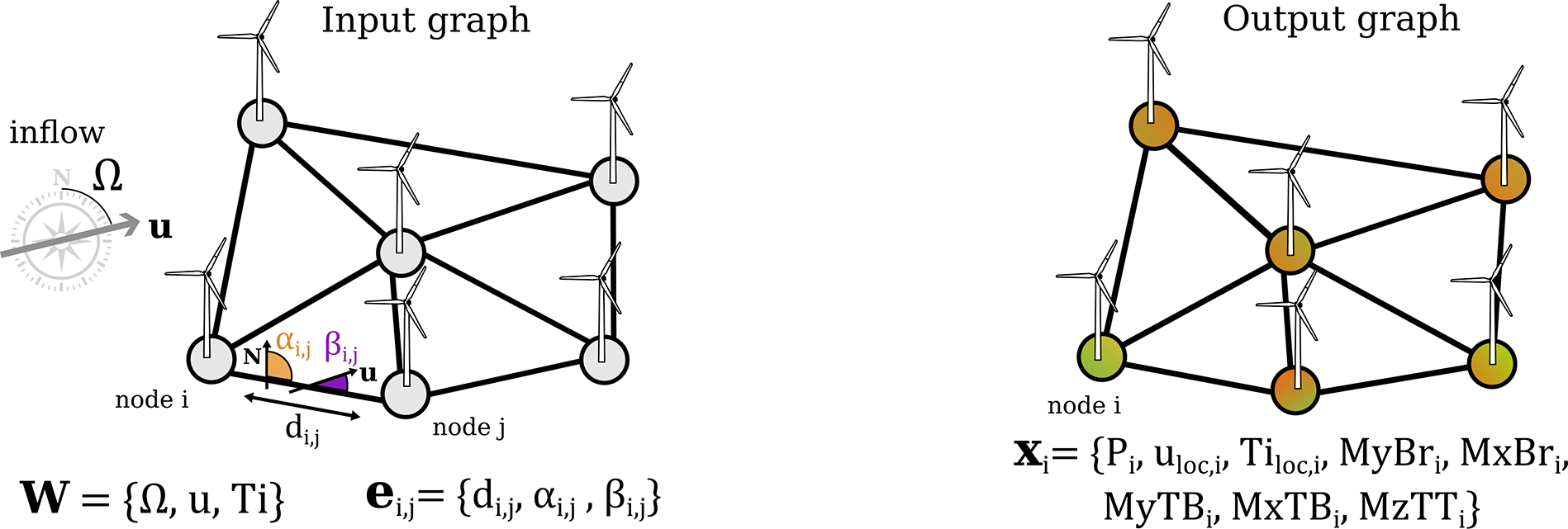
One of the two main inputs to our model is the ensemble of variables which characterize the inflow conditions. We treat these inflow variables, namely the wind direction
 $ \Omega $
, the wind velocity
$ \Omega $
, the wind velocity
 $ u $
, and the turbulence intensity
$ u $
, and the turbulence intensity
 $ {T}_i $
, as a vector of global attributes
$ {T}_i $
, as a vector of global attributes
 $ \mathbf{W} $
, i.e. attributes that have an effect on all nodes of the graph
$ \mathbf{W} $
, i.e. attributes that have an effect on all nodes of the graph
 $ \mathcal{G} $
. The other main input to our model is the geometric description of a given wind farm. This information is passed to the model via a vector of attributes
$ \mathcal{G} $
. The other main input to our model is the geometric description of a given wind farm. This information is passed to the model via a vector of attributes
 $ {\mathbf{e}}_{i,j} $
for each edge
$ {\mathbf{e}}_{i,j} $
for each edge
 $ {e}_{i,j}\in \mathrm{\mathcal{E}} $
which describes the relative positions of the nodes. In particular, each edge connecting two nodes
$ {e}_{i,j}\in \mathrm{\mathcal{E}} $
which describes the relative positions of the nodes. In particular, each edge connecting two nodes
 $ i $
and
$ i $
and
 $ j $
has an attribute vector that stores three quantities: the distance between two nodes
$ j $
has an attribute vector that stores three quantities: the distance between two nodes
 $ {d}_{i,j} $
, the angle of the edge with regard to the global north
$ {d}_{i,j} $
, the angle of the edge with regard to the global north
 $ {\alpha}_{i,j} $
and the angle of the edge with regard to the inflow direction
$ {\alpha}_{i,j} $
and the angle of the edge with regard to the inflow direction
 $ {\beta}_{i,j} $
.
$ {\beta}_{i,j} $
.
We treat the problem as a node regression task, where the model outputs 8 target features for each node. For each node
 $ {v}_i\in \mathcal{V} $
, the features of the output vector
$ {v}_i\in \mathcal{V} $
, the features of the output vector
 $ {\mathbf{x}}_i $
following: power
$ {\mathbf{x}}_i $
following: power
 $ {P}_i $
, local wind speed
$ {P}_i $
, local wind speed
 $ {u}_{loc,i} $
, local turbulence intensity
$ {u}_{loc,i} $
, local turbulence intensity
 $ {Ti}_{loc,i} $
, blade flapwise DEL
$ {Ti}_{loc,i} $
, blade flapwise DEL
 $ {MyBr}_i $
, blade edgewise DEL
$ {MyBr}_i $
, blade edgewise DEL
 $ {MxBr}_i $
, fore-aft tower DEL
$ {MxBr}_i $
, fore-aft tower DEL
 $ {MyTB}_i $
, side-to-side tower DEL
$ {MyTB}_i $
, side-to-side tower DEL
 $ {MxTB}_i $
and tower top torsional DEL
$ {MxTB}_i $
and tower top torsional DEL
 $ {MzTT}_i $
. The input and output graphs and their features are displayed in Figure 7.
$ {MzTT}_i $
. The input and output graphs and their features are displayed in Figure 7.
Features of the input and output graphs. At the input, there are no node features only global inflow features and geometrical edge features. At the output, we obtain 8 features for each turbine node.
All features—both input and target— are normalized before training. We use the statistics (mean and standard deviation) computed on the entire training set to standardize each variable.
5.2. GNN architecture
The objective of this framework can be treated as a multivariate node regression task, where the graph connectivity and graph-level attributes are given, but where no node information is known a priori:
 $$ {X}_{estimated}=\mathrm{GNN}\left(\mathcal{V},\mathrm{\mathcal{E}},\mathbf{E},\mathbf{W}\right) $$
In this section, we describe the individual components of the framework required to perform this task.
5.2.1. Encode-Process-Decode structure
Building on the approach outlined in Sanchez-Gonzalez et al. (Reference Sanchez-Gonzalez, Godwin, Pfaff, Ying, Leskovec and Battaglia2020), our study also employs an Encode-Process-Decode GNN architecture. This architecture choice facilitates message-passing operations in a latent space characterized by significantly higher dimensionality compared to the physical parameter space. Such increased dimensionality notably enhances the GNN’s capacity for complex representation, therefore increasing its potential expressivity. This design allows the network to capture intricate patterns and relationships in the data, which could be particularly advantageous for complex physics-based problem-solving tasks, such as predicting non-linear wake-induced loads. A visual representation of the proposed GNN method is shown in Figure 8.
Graphical overview of the proposed GNN framework. We use an Encode-Process-Decode structure with GEN message-passing. Each message-passing layer within the Processor uses a separate MLP to update the latent node features.
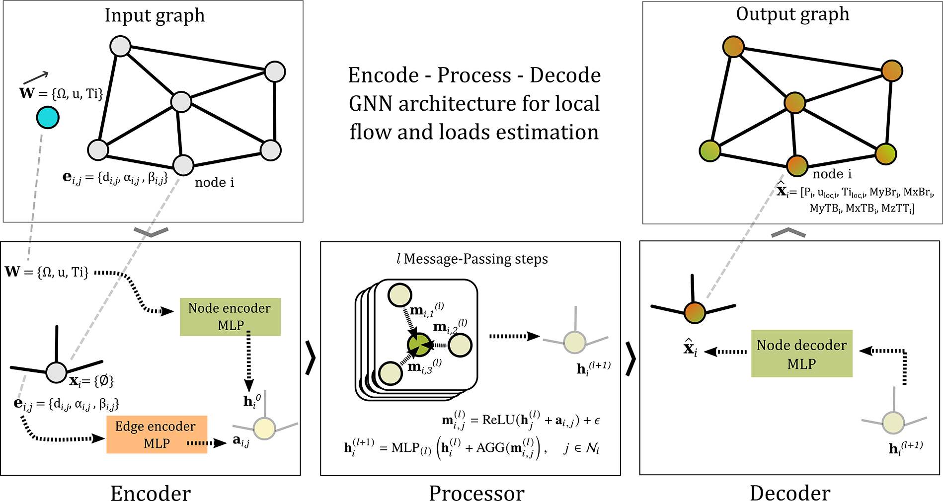
5.2.2. Encoding into a high-dimensional latent space
To operate within an
 $ N $
-dimensional latent space, graph attributes initially undergo a preprocessing step via an encoding layer. This layer comprises three distinct ReLU-activated Multilayer Perceptrons (MLPs), each containing two hidden layers. Specifically, the Edge-Encoder processes the edge features, transforming them into encoded edge vectors denoted as
$ N $
-dimensional latent space, graph attributes initially undergo a preprocessing step via an encoding layer. This layer comprises three distinct ReLU-activated Multilayer Perceptrons (MLPs), each containing two hidden layers. Specifically, the Edge-Encoder processes the edge features, transforming them into encoded edge vectors denoted as
 $ {\mathbf{a}}_{i,j} $
. Concurrently, the Node-Encoder focuses on the inflow global vector
$ {\mathbf{a}}_{i,j} $
. Concurrently, the Node-Encoder focuses on the inflow global vector
 $ W $
to produce the latent node features
$ W $
to produce the latent node features
 $ {\mathbf{h}}_i $
. The encoding process can be therefore be expressed as:
$ {\mathbf{h}}_i $
. The encoding process can be therefore be expressed as:
 $$ {\mathbf{h}}_i^{(0)}={\mathrm{MLP}}_{ENC, node}\left(\mathbf{W}\right),\hskip1em {\mathbf{a}}_{i,j}={\mathrm{MLP}}_{ENC, edge}\left({\mathbf{e}}_{i,j}\right) $$
5.2.3. Message-passing processor
The message-passing procedure serves as the foundational element in the GNN algorithm (Gilmer et al., Reference Gilmer, Schoenholz, Riley, Vinyals and Dahl2017). This involves a dual-phase approach for updating node attributes. Each message-passing layer of the Processor first calculates messages
 $ {\mathbf{m}}_{i,j} $
across all edges,; these are then aggregated at nodes using pooling functions such as max or mean. Algorithm 1 provides an overview of these steps.
$ {\mathbf{m}}_{i,j} $
across all edges,; these are then aggregated at nodes using pooling functions such as max or mean. Algorithm 1 provides an overview of these steps.
Algorithm 1 Message-passing layer
 $ l $
$ l $
for
 $ {e}_{i,j}\in \mathrm{\mathcal{E}} $
do
$ {e}_{i,j}\in \mathrm{\mathcal{E}} $
do
 $ \vartriangleright $
For each edge, compute a message
$ \vartriangleright $
For each edge, compute a message
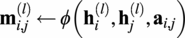 $ {\mathbf{m}}_{i,j}^{(l)}\leftarrow \phi \left({\mathbf{h}}_i^{(l)},{\mathbf{h}}_j^{(l)},{\mathbf{a}}_{i,j}\right) $
 $ \vartriangleright $
 $ \phi $
is the message update function, often a neural network
$ \phi $
is the message update function, often a neural network
end for
for
 $ {v}_i\in V $
do
$ {v}_i\in V $
do
 $ \vartriangleright $
For each node, update the features
$ \vartriangleright $
For each node, update the features
 $ {\mathbf{agg}}_i\leftarrow \mathrm{AGG}\left({\mathbf{m}}_{i,j}^{(l)}\right),j\in {\mathcal{N}}_i $
 $ \vartriangleright $
Permutation-invariant aggregation of messages (e.g. sum)
$ \vartriangleright $
Permutation-invariant aggregation of messages (e.g. sum)
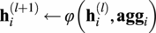 $ {\mathbf{h}}_i^{\left(l+1\right)}\leftarrow \varphi \left({\mathbf{h}}_i^{(l)},{\mathbf{agg}}_i\right) $
 $ \vartriangleright $
 $ \varphi $
is the node update function, often a neural network
$ \varphi $
is the node update function, often a neural network
end for
In this work, we adopt the GENeralized Aggregation Networks (GEN) (Li et al., Reference Li, Xiong, Thabet and Ghanem2020a) message-passing setup. GEN is a variant of the popular Graph Convolution Network (Welling and Kipf, Reference Welling and Kipf2016), which allows for edge features and other more advanced message aggregation
 $ \mathrm{AGG} $
functions. The GEN message-passing update for layer
$ \mathrm{AGG} $
functions. The GEN message-passing update for layer
 $ l $
writes:
$ l $
writes:
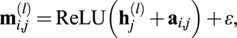 $$ {\mathbf{m}}_{i,j}^{(l)}=\mathrm{ReLU}\left({\mathbf{h}}_j^{(l)}+{\mathbf{a}}_{i,j}\right)+\varepsilon, $$
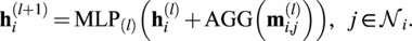 $$ {\mathbf{h}}_i^{\left(l+1\right)}={\mathrm{MLP}}_{(l)}\left({\mathbf{h}}_i^{(l)}+\mathrm{AGG}\left({\mathbf{m}}_{i,j}^{(l)}\right)\right),\hskip1em j\in {\mathcal{N}}_i. $$
where
 $ \varepsilon $
is a small positive constant, typically set to
$ \varepsilon $
is a small positive constant, typically set to
 $ {10}^7 $
. In our implementation we use the softmax type aggregation function, which can be expressed as:
$ {10}^7 $
. In our implementation we use the softmax type aggregation function, which can be expressed as:
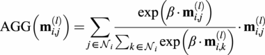 $$ \mathrm{AGG}\left({\mathbf{m}}_{i,j}^{(l)}\right)=\sum \limits_{j\in {\mathcal{N}}_i}\frac{\exp \left(\beta \cdot {\mathbf{m}}_{i,j}^{(l)}\right)}{\sum_{k\in {\mathcal{N}}_i}\exp \left(\beta \cdot {\mathbf{m}}_{i,k}^{(l)}\right)}\cdot {\mathbf{m}}_{i,j}^{(l)} $$
We choose to employ this specific message-passing formulation, based on previous results (de N Santos et al., Reference de N Santos, Duthé, Abdallah, Réthoré, Weijtjens, Chatzi and Devriendt2024a). When compared against two other popular architectures, the Graph Attention Network (GAT, Veličković et al. (Reference Veličković, Cucurull, Casanova, Romero, Lio and Bengio2017)) and the Graph Isomorphism Network with Edges (GINE, Xu et al. (Reference Xu, Hu, Leskovec and Jegelka2018); Hu et al. (Reference Hu, Liu, Gomes, Zitnik, Liang, Pande and Leskovec2019)), the GEN layer was found to be the best performing layer out of the three. Indeed for this specific problem, the GAT layer suffers from latent space collapse, while the GINE model appears to be too sensitive to inflow variability.
5.2.4. Projecting back onto the physical domain
After the
 $ L $
message-passing steps, the decoding layer functions to extract final physical quantities from the latent node features. Structurally akin to the encoder, this layer consists of a ReLU-activated MLP with two hidden layers. In essence, this step translates the high-dimensional latent features back into a physically interpretable space. The decoding step is formalized as:
$ L $
message-passing steps, the decoding layer functions to extract final physical quantities from the latent node features. Structurally akin to the encoder, this layer consists of a ReLU-activated MLP with two hidden layers. In essence, this step translates the high-dimensional latent features back into a physically interpretable space. The decoding step is formalized as:
 $$ {\hat{\mathbf{x}}}_i={\mathrm{MLP}}_{DEC, node}\left({\mathbf{h}}_i^{(L)}\right) $$
5.2.5. Pre-training the baseline general GNN
Our GNN framework is implemented using the Pytorch (Paszke et al., Reference Paszke2019) and PyTorch-Geometric (Fey and Lenssen, Reference Fey and Lenssen2019) python packages. Our baseline model is constructed with a latent dimensionality of 250, 4 message-passing GEN layers and 2 hidden-layer MLPs for the node and edge encoders as well as for the Node decoder. This yields a baseline model with a total of around 1,385,500 trainable parameters. The model is trained to minimize an
 $ L2 $
loss for all output variables over 150 epochs using the Adam optimizer (Kingma and Ba, Reference Kingma and Ba2014). The initial learning rate is set to
$ L2 $
loss for all output variables over 150 epochs using the Adam optimizer (Kingma and Ba, Reference Kingma and Ba2014). The initial learning rate is set to
 $ 1\mathrm{e}-3 $
and is annealed during training using a cosine scheme (Loshchilov and Hutter, Reference Loshchilov and Hutter2016).
$ 1\mathrm{e}-3 $
and is annealed during training using a cosine scheme (Loshchilov and Hutter, Reference Loshchilov and Hutter2016).
5.3. Fine-tuning GNNs
Given a model, constructed as described in subsection 7.1, and trained on the PyWake dataset, we aim now to fine-tune this model for the dataset of Lillgrund farm simulations described in subsection 4.2. This is a challenging task, where the difficult is twofold. Not only is the HAWC2 data of a higher fidelity and complexity, but the turbines themselves are different. This difference in the model of the simulated turbine has a major impact on the absolute values of the quantities we are interested in, proper normalization is essential. Given this challenge, we chose to test three different approaches to perform the fine-tuning, comparing each against a baseline non-pretrained ‘Scratch’ model. Table 5 summarizes the properties of the different methods, which we then describe below.
Details of the different fine-tuning methods
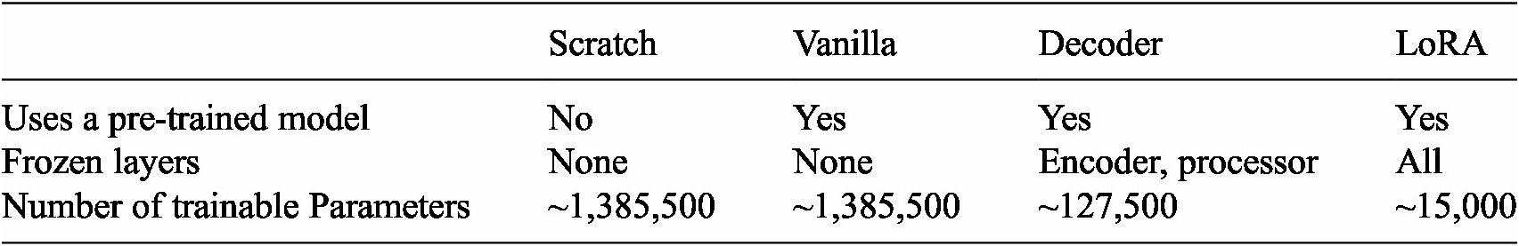
5.3.1. Vanilla
The most straightforward method for fine-tuning, which we denominate as the ‘Vanilla’ method, is to simply take the pre-trained model and re-train it on the new data. In this case, no weights of the model are frozen and all layers are trained using the higher-fidelity dataset.
5.3.2. Decoder only
Another possibility is to fine-tune only certain predefined parts of the model. In our fine-tuning task the inputs (global wind direction, wind speed and turbulence intensity) do not change, however because of the difference in turbine models between the two datasets, the output quantities are vastly different. Therefore, it makes sense to only tune the final output network, i.e. the decoder, whilst keeping the rest of the model frozen. This method can also be thought of in terms of feature extraction.
5.3.3. Low rank adaptation
Low rank adaptation (LoRA) (Hu et al., Reference Hu2021) is a recent method for more efficient fine-tuning, originally developed for large language models (LLMs) with billions of parameters. LoRA freezes the pre-trained model weights and injects trainable rank decomposition matrices into each linear layer of the model. The authors suggest that changes in the model weights during fine-tuning have a “low intrinsic rank,” and thus one can reduce the memory footprint of the model by only updating low-rank approximations of the changes
 $ \Delta $
for of all dense layer weight matrices instead of updating the full-rank matrices. Thus, for a pre-trained weight matrix
$ \Delta $
for of all dense layer weight matrices instead of updating the full-rank matrices. Thus, for a pre-trained weight matrix
 $ {W}_0\in {\mathrm{\mathbb{R}}}^{d\times p} $
, its update is constrained by representing it using a low-rank decomposition:
$ {W}_0\in {\mathrm{\mathbb{R}}}^{d\times p} $
, its update is constrained by representing it using a low-rank decomposition:
 $$ {W}_0+\Delta W={W}_0+ BA $$
where
 $ B\in {\mathrm{\mathbb{R}}}^{d\times r} $
,
$ B\in {\mathrm{\mathbb{R}}}^{d\times r} $
,
 $ A\in {\mathrm{\mathbb{R}}}^{r\times p} $
, and
$ A\in {\mathrm{\mathbb{R}}}^{r\times p} $
, and
 $ r $
is the rank of the decomposition. For all testing we use a rank
$ r $
is the rank of the decomposition. For all testing we use a rank
 $ r=4 $
. Throughout the fine-tuning process,
$ r=4 $
. Throughout the fine-tuning process,
 $ {W}_0 $
is frozen and does not receive gradient updates, whilst
$ {W}_0 $
is frozen and does not receive gradient updates, whilst
 $ A $
and
$ A $
and
 $ B $
both contain trainable parameters. During the forward pass, both
$ B $
both contain trainable parameters. During the forward pass, both
 $ {W}_0 $
and
$ {W}_0 $
and
 $ \Delta W= BA $
are multiplied with the same input, and their respective output vectors are summed coordinate-wise. For
$ \Delta W= BA $
are multiplied with the same input, and their respective output vectors are summed coordinate-wise. For
 $ h={W}_0x $
, the modified forward pass in LoRA would be:
$ h={W}_0x $
, the modified forward pass in LoRA would be:
 $$ h={W}_0x+(BA)x $$
This mathematical formulation allows LoRA to be memory-efficient while maintaining or even improving performance compared to full fine-tuning (Vanilla). As LoRA is a linear parametrization, for deployment the trainable matrices can be merged with the frozen pre-trained weights, thus yielding no additional inference overhead.
5.3.4. Fine-tuning implementation
Again, we use PyTorch to implement the different fine-tuning methods. All fine-tuned models are trained by minimizing a
 $ L2 $
reconstruction loss between the HAWC2Farm outputs and the GNN outputs. We train the models for 200 epochs using an initial learning rate of
$ L2 $
reconstruction loss between the HAWC2Farm outputs and the GNN outputs. We train the models for 200 epochs using an initial learning rate of
 $ 5\mathrm{e}-3 $
that is annealed during training with a cosine scheduler. For the LoRA model, we employ a minimal implementation of the original method, named minLoRA (Chang, Reference Chang2023).
$ 5\mathrm{e}-3 $
that is annealed during training with a cosine scheduler. For the LoRA model, we employ a minimal implementation of the original method, named minLoRA (Chang, Reference Chang2023).
6. Results
In the present section, we proceed to analyse the expressiveness of GNNs in capturing fundamental physical behaviour on wind farms. We initiate by assessing the base performance of the pre-trained GNN model on the lower resolution PyWake data. We then focus on the fine-tuning performance, specifically addressing which approach (LoRA, Vanilla, Decoder or Scratch) is preferable, as a function of the amount of available training data. We then discuss in detail the results in relation to the each predicted quantity and the overall farm fatigue patterns. Finally, we identify relative pitfalls, and study possible mitigation strategies.
6.1. GNN predictions for PyWake data
We first aim to confirm that the baseline model, trained on the PyWake dataset, sufficiently captures the simulated behavior of a wind farm. In Figure 9, we plot for an unseen random wind farm layout, the different outputted quantities of the GNN against those given by the PyWake simulator for two turbines in a range of inflow conditions in all wind directions (every 5° from 0° to 360°). We observe that the GNN predictions closely align with those given by PyWake.
Polar plots of the outputs of the baseline GNN (trained only on the PyWake data) versus the PyWake simulation outputs as a function of wind direction for an unseen random farm layout with 720 inflow conditions (10 inflow velocities per 5° sector). We show the outputted quantities for two turbines on opposite sides of the farm (WT 51 in blue and WT 12 in orange). Shaded surfaces indicate 5% variance around the mean.
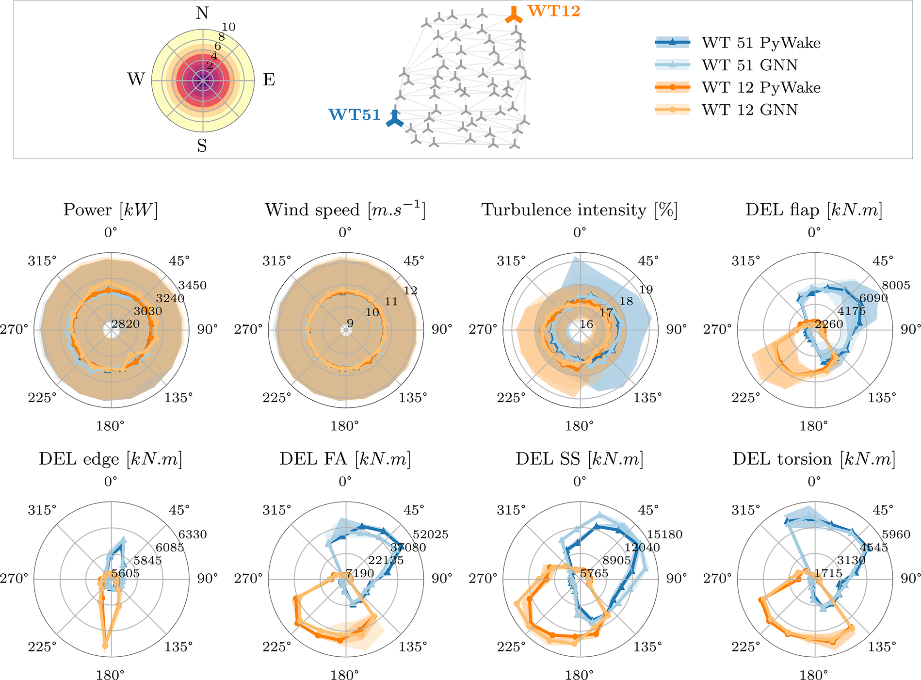
This polar plot is of particular interest as it not only demonstrates a good agreement between the GNN model predictions and the simulated PyWake quantities, but further allows deeper insights into the farm wake physics and how the GNN model is capturing these. This is exemplified by the preponderance of N–SE sector (0°–140°) for WT51 in its turbulence intensity. It is in this region where WT51 sees its highest turbulence intensity. This has, as expected, an impact on the fatigue loads which, for pure aerodynamic simulations (e.g., no hydrodynamics) are strongly correlated with wake and, therefore, turbulence intensity. It ought however be noticed that fatigue loads are strongly non-linear, as evidenced by the plot, and phenomena like accumulating nature of the wake effect. Other loads, like the blade-root edgewise moment, which is mostly gravitational-dependent but is also influenced by some aerodynamic loads (Rinker et al., Reference Rinker, Soto Sagredo and Bergami2021), depend more on directly near-wake turbines than far-wake accumulation over the farm and are, therefore, less related to overall turbulence intensity. As for WT12, as it is diametrically opposite to WT51, its pattern of wind direction dependency for turbulence intensity and fatigue loads almost perfectly mirrors WT51 (180° inversion).
6.2. Fine-tuning
Here, we discuss in detail the different approaches for fine-tuning and their expressiveness in relation to transfer learning. As a quantitative metric for most of our results we use the Mean Absolute Percentage Error (MAPE), which can be formulated as a function of the actual values, represented as
 $ y $
, and the predicted values, represented as
$ y $
, and the predicted values, represented as
 $ \hat{y} $
. The MAPE function is defined as follows:
$ \hat{y} $
. The MAPE function is defined as follows:
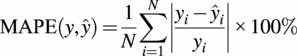 $$ \mathrm{MAPE}\left(y,\hat{y}\right)=\frac{1}{N}\sum \limits_{i=1}^N\left|\frac{y_i-{\hat{y}}_i}{y_i}\right|\times 100\% $$
where
 $ {y}_i $
denotes the actual value and
$ {y}_i $
denotes the actual value and
 $ {\hat{y}}_i $
denotes the predicted value for the
$ {\hat{y}}_i $
denotes the predicted value for the
 $ i $
-th observation out of
$ i $
-th observation out of
 $ N $
total observations. One must however be aware that when the true value lies close to zero, even small errors may lead to disproportionately large percentage errors. In our case, the only predicted value which may be zero is power, as such when computing the MAPE for power we exclude cases where no power is produced.
$ N $
total observations. One must however be aware that when the true value lies close to zero, even small errors may lead to disproportionately large percentage errors. In our case, the only predicted value which may be zero is power, as such when computing the MAPE for power we exclude cases where no power is produced.
6.2.1. Overall performance of the different fine-tuning methods
Given the four different approaches described in Table 5, we can compare their relative performance. Here, it is relevant to highlight that the Scratch approach, wherein there is no transfer learning and no use of a pre-trained model (the GNN is trained directly on the available data), serves as the baseline to which each model compares itself. The publicly available dataset described in subsection 4.2 is comprised of 800 HAWC2 aeroelastic simulations. Of these, 200 simulations are saved to test the performance of the trained models. The rest of the available data is pooled and used to train the model in different sample sizes (2–500), to demonstrate the effectiveness of each method given a certain number of training samples and to discern what is the minimal amount of samples required to reach a set prediction error.
In Figure 10, we perform a comparison of each method for different training sample sizes by analyzing their MAPE, aggregated for all 8 outputted variables. For every sample size, all methods are subjected to ten evaluations, with each evaluation representing a separate training run. These runs are distinct due to individual seeds that dictate the random selection of the training samples.
Comparing the different fine-tuning methods. MAPE metrics are shown as an average of each output variable, gathered on the test set with 200 samples. Solid lines indicate the mean MAPE results gathered over the 10 data splitting seeds. Violet highlight represents the 106 training samples. Shaded curves represent the 90% distribution percentile.
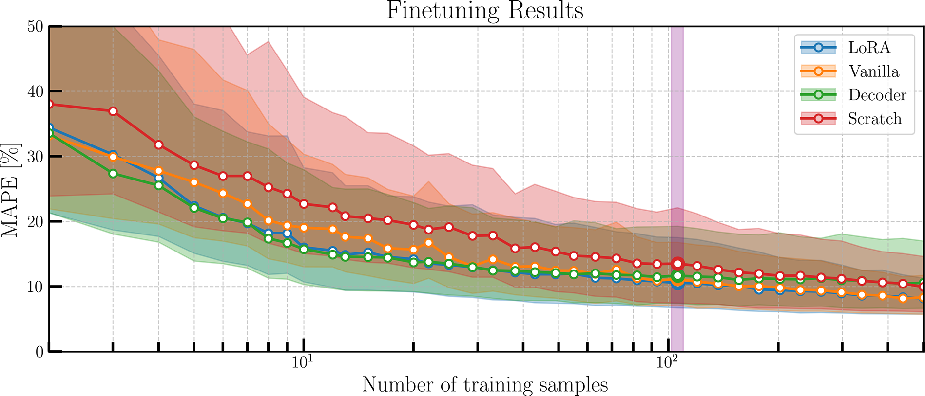
In this figure, we observe that all models converge to the same error with increasing sample sizes (around 10%). We can further observe how all methods (LoRA, vanilla and decoder) outperform training a model from scratch at all sample sizes bar the last (where the decoder models perform slightly worse). There is interestingly a inversion of the different methods’ performance around 100 samples (highlighted region, in violet): for a low amount of training samples, LoRA and the decoder-only retraining methods perform the best. However, with greater amounts of data the Decoder model stagnates, whereas the Vanilla and LoRA models continue improving. This makes sense as the number of trainable parameters of the Vanilla model are ten times greater than for decoder-only. With only the readout layer unfrozen, the decoder-only model seemingly hits a limit in its representation power for the HAWC2 dataset. Similarly, LoRA models are highly performant, as low-rank adaptation has been developed to effectively deal with billions of parameters of large models. We identify this inflection point in Figure 10 by highlighting in purple the models for 106 training samples. This is a significant number of samples because it represents a point where the Decoder’s performance stagnates and there is already a level of convergence. Additionally, this number of samples represent about half of the test dataset. In Table 6, we compare the performance of each method for each estimated variable, highlighting the best-performing model at 106 (black) and 500 (grey) samples.
Performance of the different fine-tuning methods (MAPE) for each estimated variable for two training samples sizes and averaged over all runs with different data-splitting seeds. Best performing method is highlighted for each sample size (black, 106; grey, 500). For power, MAPE scores are only computed in cases when power is produced
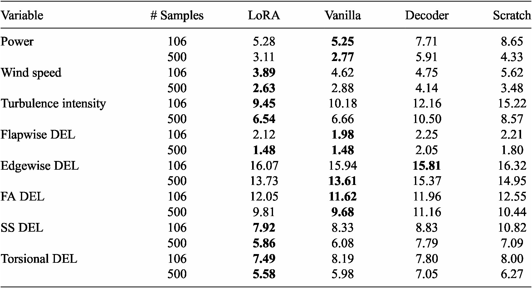
This table reveals both LoRA and the vanilla scheme as the best performing models with, generally, LoRA performing better for wind speed, turbulence intensity, side-to-side and torsional DELs, and the vanilla model performing better for power, flapwise, edgewise and fore-aft DELs. However, for both sample sizes, the errors are comparable. We further observe, for both models, a significant improvement with respect to training from scratch (for 106 this difference can be
 $ +5\% $
). Therefore, in our further analyses we focus on the best performing LoRA model for 106 samples. By analyzing a model for such a low amount of data we remain faithful to the objective of developing a generalist model which does not require great quantities of data to effective adapt to new turbines/fidelity.
$ +5\% $
). Therefore, in our further analyses we focus on the best performing LoRA model for 106 samples. By analyzing a model for such a low amount of data we remain faithful to the objective of developing a generalist model which does not require great quantities of data to effective adapt to new turbines/fidelity.
In Figure 11 we further examine the distributions of the prediction error per output quantity for all models. We can directly identify the relative difference between each predicted quantity. In general, the closer the error curves are skewed towards 0% (i.e., Weibull), the easier the quantity is to predict, e.g., power or flapwise DEL. Conversely, if the error resembles a continuous distribution, then the model has a greater difficulty to capture that quantity (e.g., edgewise DEL). Additionally, differences between each fine-tuning method are noticeable. In general, LoRA presents error distributions more skewed towards 0% than its counterparts. For example, when predicting turbulence intensity using Scratch or the decoder the error resembles a continuous distribution, whereas LoRA is closer to a Weibull.
Comparing the different fine-tuning methods with all models trained on 106 HAWC2Farm simulations. MAPE distributions gathered on the test set with 200 samples are shown for each output variable.
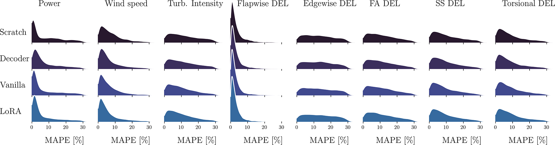
6.2.2. Model physicality
Comparing farm-level behavior
An integral part of validating the results lies in confirming their physicality, that is to say, if the results make physical sense. We posit that our GNN model is capable of learning underlying physical relationships (such as wakes) in a coarse level (PyWake) before being fine-tuned for a specific task on a higher-fidelity solver. Given our pre-training scheme, the GNN should first learn relatively before learning specifically. To verify whether our training regime does indeed allow the GNN to learn what a wake is, we plot in Figure 12 the predicted local effective turbulence intensity for each turbine of the Lillgrund farm for all models at 106 samples, for a given inflow condition.
Comparison of the predicted local effective turbulence intensity for the different models trained on 106 HAWC2Farm simulations for a single southwesterly inflow condition (9.4
 $ m.{s}^{-1} $
and 9.9% turbulence intensity). For reference, we also show the equivalent PyWake output.
$ m.{s}^{-1} $
and 9.9% turbulence intensity). For reference, we also show the equivalent PyWake output.
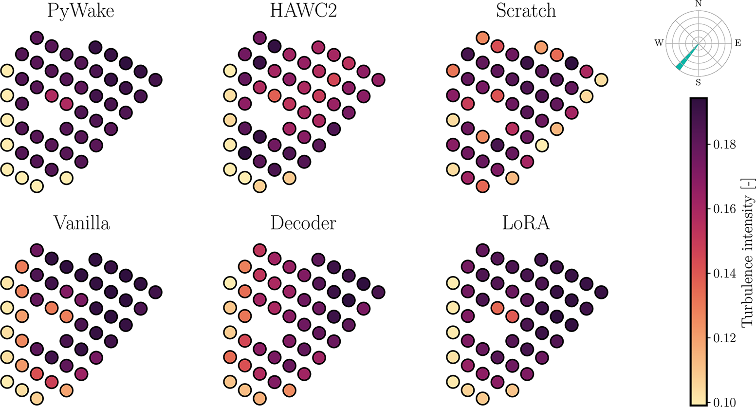
In this figure, we can observe that the Scratch model predicts an average turbulence intensity value for all turbines, indicating that it is unable to identify front-row turbines, distinguishing these as free-flow and effectively learn wake effects. However, this is not the case for the pre-trained models (Decoder, Vanilla and LoRA GNNs), indicating that pre-training with PyWake does result in better underlying physicality. However, we note that the HAWC2Farm ground truth is noticeably more nuanced than the equivalent PyWake solution, especially for the back-row turbines where the effects of multiple wakes start to stack. This is something which all GNN models do not completely capture, with only the Vanilla and LoRA models approaching the HAWC2Farm solution for the non-waked turbines. LoRA is particularly similar to HAWC2 in the first two strings, but more complex phenomena like the ‘gap’ for the 3rd and 4th rows, which in HAWC2 has an impact on all subsequent rows, making the northeasterly sector of the farm more nuanced (turbulence intensities between 14% and 17%, in orange–violet), is much more binary for LoRA (just two turbines immediately after the gap appear with a lower turbulence intensity, as in PyWake). This seems to suggest that pre-training allows model to quickly understand basic physical behaviour, like the distinction between free-flow and wake-affected turbines, but more intricate wake behaviour such as the interplay between far-wake and near-wake boundary layer recovery are not captured, mostly because the baseline simulator (PyWake) does not have the necessary resolution to address these situations.
This absence of nuance is also reflected in the predicted DELs, as shown in Figure 13. Predicting the DELs correctly is more challenging (as seen above, they are more non-linear), and here the PyWake legacy may actually be harmful. This may be observed by examining the discrepancies in the patterns between the HAWC2Farm and PyWake solutions, where the turbines with maximal predicted FA DELs do not match. While the fine-tuned GNN models do also lack nuance here, the extrema in the predictions do have better alignment with the HAWC2Farm ground truth. Here again, the model without pre-training predicts averaged out values over the entire farm.
Comparison of the predicted fore-aft damage equivalent loads for the different models trained on 106 HAWC2Farm simulations for a single southwesterly inflow condition (9.4
 $ m.{s}^{-1} $
and 9.9% turbulence intensity). For reference we also show the equivalent PyWake output using a different colormap due to the turbine model disparity.
$ m.{s}^{-1} $
and 9.9% turbulence intensity). For reference we also show the equivalent PyWake output using a different colormap due to the turbine model disparity.
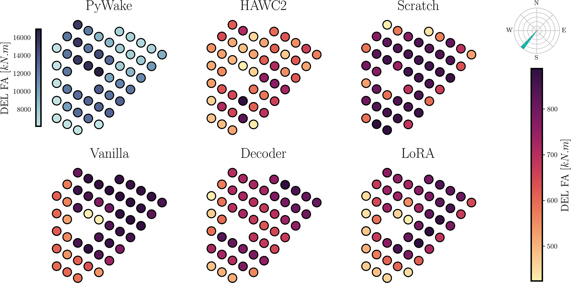
Predicting wake effects
In this section, we focus on the performance over each variable for two different turbines. We present the results for the best LoRA model at 106 samples for all variables of two turbines of the Lillgrund wind farm: a free-flow wind turbine (WT1) and a wake-affected one (WT26). In order to ensure that WT1 is fully free-stream, we restrict the wind-rose by excluding SW–NW samples (see Figure 14). In Figure 15 we can observe the difference between the true and predicted power curves for the free-stream turbine (WT1, blue–orange) and the wake-affected one (WT26, purple–dark red), along with their relative position within the Lillgrund wind farm. In this figure it can be observed how the power curve for the free-stream turbine is much higher before rated power than for the wake affected turbine, which also only achieves rated power at a higher wind speed due to the effect of turbulence. It is also recognisable that the LoRA GNN model is able to accurately model both power curves.
Power curve for free-stream turbine (WT1; blue, true; orange, predicted using LoRA) and wake-affected turbine (WT26; purple, true; dark red, predicted using LoRA). SW–NW wind direction excluded. Shaded curves represent the 75% distribution percentiles.
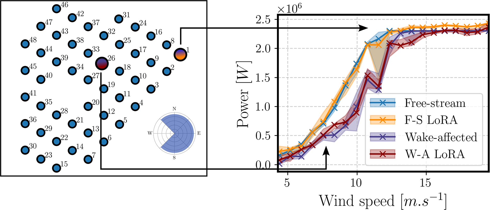
Power, wind speed, turbulence intensity, Flapwise DEL, Edgewise DEL, fore-aft (FA) DEL, side-to-side (SS) DEL and Torsional DEL curves for free-stream turbine (WT1; blue, true; orange, predicted using LoRA) and wake-affected turbine (WT26; purple, true; dark red, predicted using LoRA). SW–NW wind direction excluded. Shaded curves represent the 75% distribution percentiles.
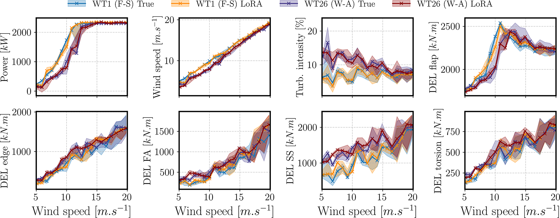
However, it should be noted in this figure that, for the free-flow turbine, the LoRA GNN model is over-predicting the power curve at rated power (wind speed above
 $ 11m.{s}^{-1} $
). This has no physical meaning, as the turbine’s power is restricted to its rated power and, therefore, the LoRA GNN model has not learned this important feature of the power curve. However, this can easily be corrected by applying a threshold. Additionally, in Figure 15, all output variables (true and predicted) are plotted for WT1 and WT26 against the global inflow wind speed. In this figure, the generalist GNN model is shown able to capture both free-stream (blue-orange) and wake-affected (purple-dark red) turbine behaviour for all variables. The model is quite capable of predicting the power curve, local wind speed and turbulence intensity. For other variables, namely some loads, like FA DEL, there are some discrepancies, but the overall trends are still being captured. We further observe that the model is able to clearly distinguish between free-stream turbines and wake-affected ones, further demonstrating that, also at a turbine-level, the fine-tuned GNN model is able to comprehend wake dynamics.
$ 11m.{s}^{-1} $
). This has no physical meaning, as the turbine’s power is restricted to its rated power and, therefore, the LoRA GNN model has not learned this important feature of the power curve. However, this can easily be corrected by applying a threshold. Additionally, in Figure 15, all output variables (true and predicted) are plotted for WT1 and WT26 against the global inflow wind speed. In this figure, the generalist GNN model is shown able to capture both free-stream (blue-orange) and wake-affected (purple-dark red) turbine behaviour for all variables. The model is quite capable of predicting the power curve, local wind speed and turbulence intensity. For other variables, namely some loads, like FA DEL, there are some discrepancies, but the overall trends are still being captured. We further observe that the model is able to clearly distinguish between free-stream turbines and wake-affected ones, further demonstrating that, also at a turbine-level, the fine-tuned GNN model is able to comprehend wake dynamics.
6.2.3. Negative transfer
A transfer learning approach is successful if it has the the ability to adjust and exploit the inductive bias of a model trained on a source task such that it outperforms a model trained from scratch on the target task. When fine-tuning, a primary focus is to avoid negative transfer, a phenomenon that arises when the model’s behavior, shaped by the optimization for the pre-training task, negatively impacts its performance on the new task. This issue often stems from the pre-existing weights and biases, initially optimized for the original tasks, not aligning with the new task’s requirements. If this misalignment is not rectified during training, it can result in sub-optimal performance. In our case, some negative transfer is apparent in Figure 14, where the model predicts a power output beyond the rated value. To understand in more detail the negative transfer present in our fine-tuning framework, we plot in Figure 16 the predictive error of the LoRA and Vanilla models against the prediction errors for the model trained from scratch on only the HAWC2Farm data. For each model, 106 samples of the high-fidelity dataset were used for training, and results were gathered on the 200 samples of the test set. The color of the points indicate the inflow wind speed. We observe that both the LoRA and the Vanilla models mostly perform better than the Scratch model, with both distributions skewing below the parity line. For both models, strong cases of negative transfer seem to occur primarily for lower wind speeds. One potential explanation for poor performance for low ambient wind speeds is the difficulty in accurately capturing the exponential behavior of the turbulence intensity when velocity is close to zero.
Side-by-side comparison of the distribution of LoRA and Vanilla MAPE results (computed by averaging MAPE over each output variable) plotted against the MAPE results of the Scratch model and colored by wind speed. Upper left parts of the plots are zones where negative transfer occurs, i.e. when pre-training harms model prediction for the downstream task. 106 training samples were used.
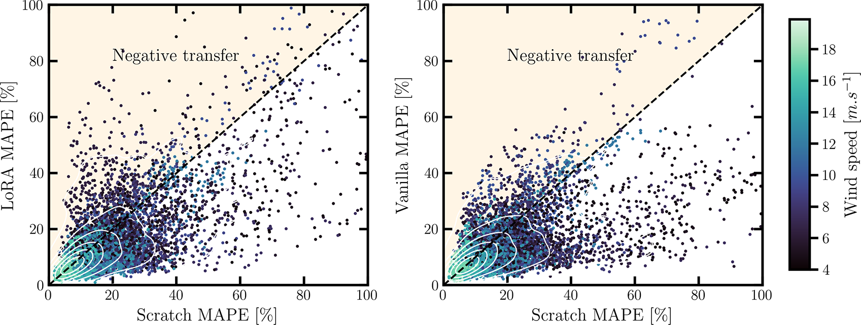
Excluding the low wind speed cases, we obtain Figure 17. In this case, we only show MAPE scores for wind speeds above rated power and color the points by inflow wind direction. From the plots we can identify particular inflow sectors which result in the worst cases of negative transfer: around 45°, 225° and 280° from North. In relation to the Lillgrund farm layout, these directions seem to correlate with the directions in which the strings of waked turbines are the longest. This is in line with our previous observation that PyWake has some difficulty modelling wake accumulation, and thus some negative legacy of the pre-training is observed.
Side-by-side comparison of the distribution of LoRA and Vanilla MAPE results filtered for rated wind-speed only (computed by averaging MAPE over each output variable) plotted against the MAPE results of the Scratch model and colored by inflow direction. 106 training samples were used.

6.3. Scaling up
In the previous section, we show that use of pre-trained models, even on data from low resolution flow simulators like PyWake, supports the GNN in learning basic wake physics and to understand the differences between free-stream and waked turbines. However, we further observe how intricate phenomena like boundary layer recuperation and wake effect accumulation over a farm are considerably more difficult to capture. Here, we attempt to improve on the GNN’s expressivity by increasing the number of trainable parameters.
Our underlying argument behind this option lies with the fact that we are developing a generalist model, which should be able to adapt to any given layout, inflow condition, turbine type and even fidelity level. Therefore, it is reasonable to expend more time and resources on the training of the model, as its application further down the line would save much more time in computational terms. We can afford this because using LoRA to fine-tune the baseline model is rather fast, especially when only around 100 samples are used for fine-tuning. For our previous baseline model, we typically get single GPU training-step times of about 10s per epoch and a max VRAM footprint of about 1.2GB, which comfortably fits on the 24GB onboard VRAM of the RTX3090 GPU that we used. Thus, a much larger model can easily be trained and fine-tuned. We design a larger model with 8 message-passing layers and encoded dimensions of 1024 for all graph attributes, which yields approximately 40M trainable parameters. This model is first trained on the PyWake dataset and then fine-tuned using LoRA and compared here against the baseline LoRA model (1M trainable parameters), allowing us to understand the performance change given by scaling-up the model.
We first gather in Table 7 prediction error metrics for all variables for the LoRA 40M model, and compare them to the results for the best run of the LoRA 1M model, both trained on 106 simulations.
Performance (MAPE) for each estimated variable for the LoRA 1M and LoRA 40M models, fine-tuned on 106 HAWC2Farm samples, using the best performing data-splitting seed. For power, MAPE scores are only computed in cases when power is produced
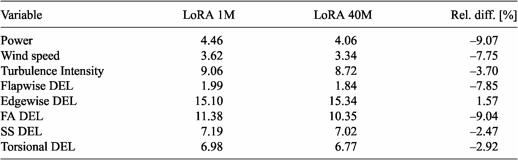
This table demonstrates that increasing the size of the model improves performance for nearly all outputs, by up to 9%, except for the edgewise blade DELs where performance is slightly degraded although still comparable. For quantities like power, wind speed, fore-aft DEL, torsional DEL or flapwise DEL, the positive change is of note.
We then further investigate the LoRA 40M model performance by showing the polar plots comparison between both LoRA models and the HAWC2Farm ground truth per variable, given the 200 testing inflow samples (Figure 18). These are plotted for WT33 (waked) according to the incoming wind direction. This turbine is selected, as it is one of the most difficult locations to capture, given that it is located just behind the ’gap’ in the middle of the farm. In line with Table 7, the biggest improvements are seen for the fore-aft and torsional DELs, specifically around 135°. The highest errors occur for the edgewise DEL, with the largest over-prediction occurring for inflows around 180°. As previously mentioned, edgewise DELs are particularly difficult to capture due to their, in part, near-wake dependency and strongly non-linear behaviour.
Polar plots of the predicted outputs averaged per wind direction for the LoRA 1M and LoRA 40M models trained on 106 HAWC2Farm simulations for a single center turbine of the Lillgrund farm.
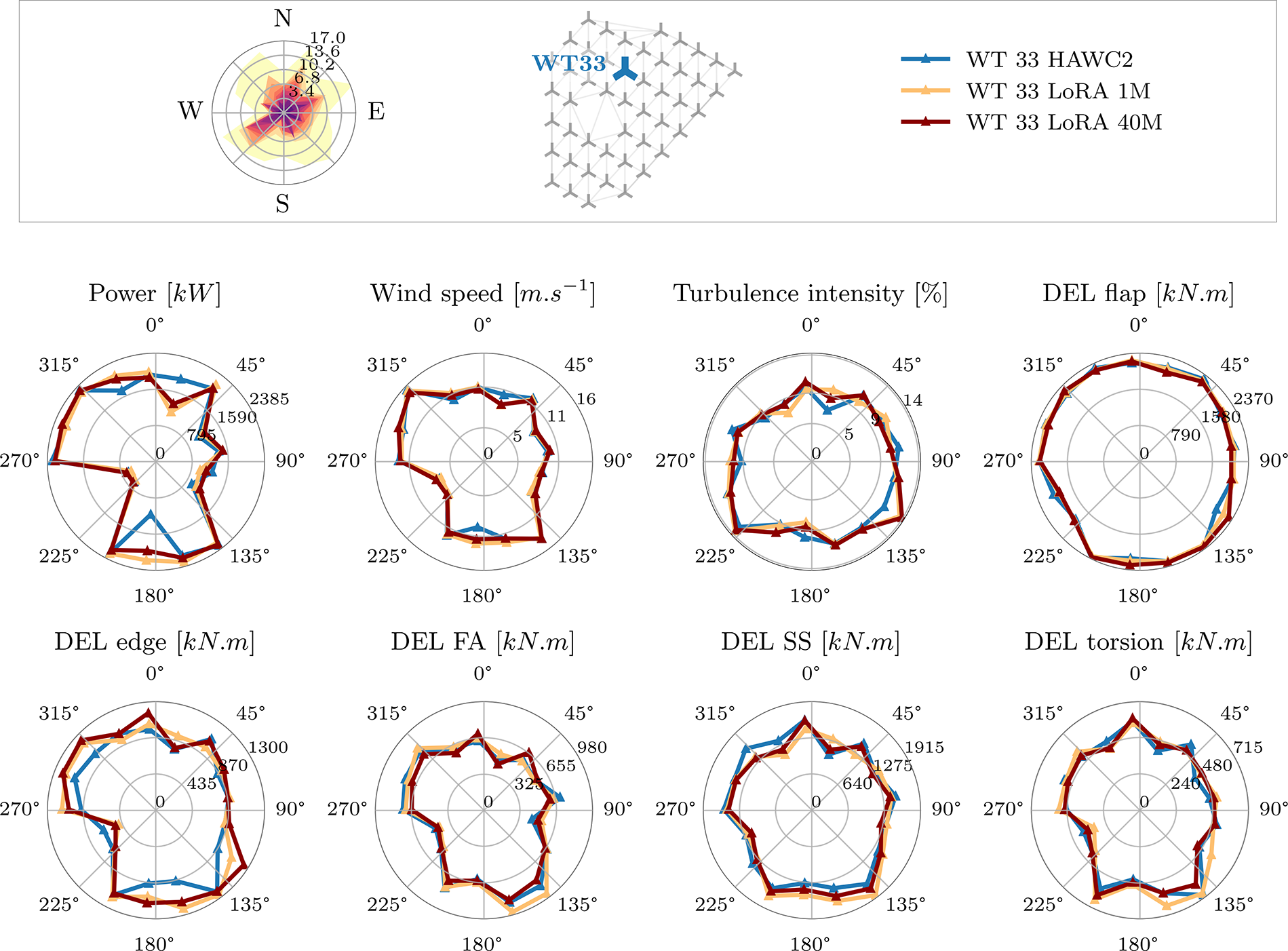
We can finally spatially compare the farm-level behavior of the LoRA 1M, LoRA 40M and HAWC2 (ground truth), by plotting the farm predictions for each model in Figure 19. In this figure, we observe that an increased number of trainable parameters of the LoRA 40M model improves the spatial representativeness of the model. Specifically, immediately after the gap in the middle of the farm we notice how the original LoRA 1M model had an almost binary distinction for that region, with turbines in the vicinity of the gap in yellow, succeeded by an almost immediate over-prediction of loads. The overestimation phenomenon is transversal to the farm. As for LoRA 40M, despite some overestimation, it is better able to represent the nuance of fore-aft loading throughout the farm, especially for the back-row turbines and the overall overestimation is attenuated.
Comparison of the predicted fore-aft damage equivalent loads for the LoRA 1M and LoRA 40M models trained on 106 HAWC2Farm simulations for a single southwesterly inflow condition (9.4
 $ m.{s}^{-1} $
and 9.9% turbulence intensity).
$ m.{s}^{-1} $
and 9.9% turbulence intensity).
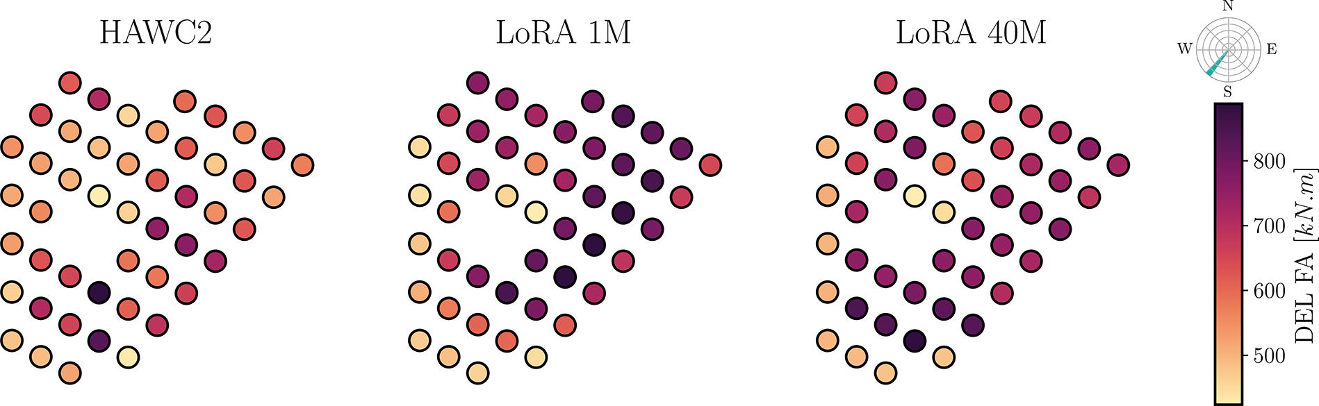
7. Discussion and conclusions
In this contribution, we present a predictive modelling approach at the level of wind turbine farms, seen as populations of structures that are represented by a graph. Specifically, we tackle the well-known Lillgrund offshore farm. To this end, we develop a ‘generalist’ graph neural network model first trained on relatively inexpensive numeric simulations from PyWake. We then fine-tune the model using a small amount of higher fidelity HAWC2Farm simulations of the target wind farm and turbine. This approach allows us to capitalize on the transfer learning capabilities of GNN, enabling training on inexpensive simulations before specializing the model for accurate prediction with higher fidelity data. Specifically, we compare four possible modeling strategies: training from scratch, fully re-training a pre-trained model (Vanilla), freezing all layers of the pre-trained model and just re-training the decoder ones, and employing low-rank adaptation (LoRA). Amongst these four approaches, we observe that LoRA and the Vanilla approach produce the best results, both in terms of overall percentage error, error per variable, and the capability of capturing spatial patterns (i.e., the load distribution over the farm). Both the LoRA and Vanilla models require lower amounts of data when fine-tuning than the Scratch and Decoder models to achieve the same accuracy levels. We furthermore observed that the inclusion of a pre-trained model significantly improves results, especially for layout pattern resolution when compared to training from scratch. Moreover, having access to the pre-trained model reduces the amount of data required to train a model in order to reach acceptable accuracy.
Thereafter, we focused on the physicality of the LoRA model for 106 training samples (half of the test samples), and observe a sufficiently precise prediction for all variables of interest (e.g., the power curve). We further analyze the proposed model’s performance by testing for negative transfer and ensuring that it remains low. Finally, in order to increase spatial expressivity, we train a LoRA model with ×40 more trainable parameters than the original LoRA model, with increased performance and better nuance on the farm-wide loading patterns.
This work introduces a powerful graph-based framework to fine-tune a flexible generalist model that can account for specific wind farm site layouts, different turbine types, and even diversified levels of simulation fidelity. This investigation further unveils current limitations. Complex wake behavior (boundary layer recuperation, near-wake effects, and wake effect accumulation) is better captured by the higher fidelity simulations. The goal of our transfer learning approach is to capture such complex physics while using low amounts high-fidelity data to do so, rather than simply training a surrogate model from scratch. In this contribution we demonstrate precisely this while, at the same time, establishing the limits of such an approach: not all intricacies of the more complex physics of the higher-fidelity simulations are captured by the model, despite the pre-training giving the model a good understanding of the basic physics (e.g., distinguishing between free-flow and wake-affected turbines). This is evident in the accumulation of wake effects throughout the farm and the corresponding influence of changes in the geometry (e.g., a gap in a row).
We attempt to circumvent this issue by increasing the pre-trained model’s training parameters, with an increased performance and better nuance. However, we further notice that we are reaching the limits of the pre-training using the inexpensive flow simulator (PyWake) in terms of its ability to simulate wake physics. It is non-trivial to expect a model to learn intricate physical nuances not contained in its original pre-training dataset by simply fine-tuning. This, especially, using only 100 samples for the re-training of the model, while having to fine-tune for a new turbine type, with a different rotor size, which also impacts wake dynamics. A straightforward solution is to simply increase the number of mid- to high-fidelity samples used for fine-tuning or, even, pre-training a model on mid-fidelity simulators like HAWC2. Nonetheless, we can think of a more refined form of ‘curriculum’ training of this overarching GNN model in the future, one that is able to adapt to any new layout/turbine type, by dividing model pre-training into two stages. First, a stage of low-fidelity simulations (PyWake) can be used to train the GNN model and enable it to quickly learn fundamental (i.e., ‘easy’) physics like distinguishing between free-flow and wake affected turbines for a wide range of wind speeds, turbulence intensities, and different pseudo-layouts. In a second stage, the GNN model can be trained on mid-fidelity simulations (HAWC2), in a quantity and diversity sufficient for it to learn more intricate physical phenomena, not present in PyWake: the mechanics of boundary layer recuperation, near-wake effects, etc. We leave these refinements to be explored in future work.
The work presented in this contribution has the potential to be a powerful contributor for further advancements, such as accelerating layout design, optimizing wind farm instrumentation, and developing fatigue-aware control strategies. The introduced GNN framework, with its flexibility and low computational cost, could serve as a tractable surrogate that can be coupled with demanding optimization techniques like reinforcement learning. Furthermore, the automatic calculation of gradients by the GNN surrogate enables the use of gradient-based methods to develop new optimal control strategies, such as load-aware wake steering or curtailment. This synergy between GNN surrogates and optimization algorithms promises to enhance the overall performance and longevity of wind farms, balancing power generation with fatigue management.
Acknowledgements
We are grateful for the technical assistance of Pierre-É louan Rethoré (DTU) with PyWake.
Author contribution
Conceptualization: G.D.; F.d.N.S.; I.A.; E.C. Methodology: G.D.; F.d.N.S.; I.A. Formal Analysis: G.D.; F.d.N.S. Data curation: G.D.; F.d.N.S.; I.A. Data visualisation: G.D.; F.d.N.S. Writing – Original draft: G.D.; F.d.N.S. Writing – Reviewing & Editing: I.A.; W.W.; E.C; C.D. Funding Acquisition: E.C.; C.D. All authors approved the final submitted draft.
Competing interest
The authors declare no competing interests exist.
Data availability statement
We provide the associated code and pre-trained models at https://github.com/gduthe/windfarm-gnn. Furthermore, the dataset of PyWake simulations used for pre-training can be accessed in de N Santos et al. (Reference de N Santos, Duthé, Abdallah, Réthoré, Weijtjens, Chatzi and Devriendt2023a).
Funding statement
This work was supported by the BRIDGE Discovery Program of the Swiss National Science Foundation and Innosuisse (Grant No. 40B2-0_187087), as well as the French-Swiss project MISTERY funded by the French National Research Agency (ANR PRCI Grant No. 266157) and the Swiss National Science Foundation (Grant No. 200021L_212718). The authors would also like to acknowledge the Fonds Wetenschappelijk Onderzoek – Vlaanderen (FWO) for its long stay abroad grant (Grant No. V434422N).
Ethical standard
The research meets all ethical guidelines, including adherence to the legal requirements of the study country.


 Open access
Comments
No Comments have been published for this article.