Introduction

Reference DansgaardDansgaard (1964) showed that stable isotopes of water contain information about the hydrological cycle, and consequently bring valuable climatic information from virtually all forms of paleoclimate archives linked to water in its different states. Among the most used archives for water isotopes are ice cores. As noted in the first studies of the hydrological cycle using ice-core records (Reference LangwayLangway, 1967), the seasonal amplitude of δ¹⁸O decreases with depth and time. This effect is due to diffusion within the ice matrix, and especially between the air-filled pores of the firn layer, which tends to smooth the record with time. The principal description of diffusion was given by Reference FickFick (1855), and details of the process of diffusion of stable water isotopes in firn and ice were first described by Reference JohnsenJohnsen (1977), and subsequently by Reference Whillans and GrootesWhillans and Grootes (1985), Reference Cuffey and SteigCuffey and Steig (1998) and Reference Johnsen, Clausen, Cuffey, Hoffmann and SchwanderJohnsen and others (2000).

This effect of diffusion smoothing of short-timescale or high-frequency variability, often regarded as noise, will dampen, and finally erase the record of, lower frequencies such as the annual signals. Provided the isotope measurements are accurate enough, such that a sufficient signal-to-noise ratio remains to preserve the annual signal, the diffusion equations can be inverted with respect to time, and the ice-core records can be back-diffused (or deconvoluted) by numerical operations (Reference JohnsenJohnsen, 1977; Reference Bolzan and PohjolaBolzan and Pohjola, 2000; Reference Johnsen, Clausen, Cuffey, Hoffmann and SchwanderJohnsen and others, 2000), to reveal close-to-original amplitudes.

In this work, we investigate how well the current theories of vapor-driven diffusion describe the diffusion rate in firn, by comparing calculated diffusion rates with diffusion rates measured in firn during a controlled laboratory experiment. We further test and evaluate three different analytical and numerical methods used to solve the diffusion equation. Our results will serve as an aid for estimating limits for using back-diffusion techniques on ice-core records.

Theory

The time-dependent general diffusion equation, known as Fick’s second law, (Reference FickFick, 1855) has the general form:

(1)

To apply this general equation to describe isotope diffusion in ice, two steps are needed. First, the general concentration term in Equation (1) has to be specified as C = δ_i , where the index i describes the two isotopomers (i = ¹⁸O, ²H). Secondly, we have to find the expression for the general diffusion coefficient D (dimension length² time^–1). Reference Johnsen, Clausen, Cuffey, Hoffmann and SchwanderJohnsen and others (2000) gave a full explanation of the terms that make up the expression for D as

(2)

This expression is developed from the Reference JohnsenJohnsen (1977) and Reference Whillans and GrootesWhillans and Grootes (1985) models. Intercomparisons between these models have shown that they yield approximately the same results (Reference Pohjola, Bolzan, Cuffey and JohnsenPohjola and others, 1998). Reference Johnsen, Clausen, Cuffey, Hoffmann and SchwanderJohnsen and others (2000) provided a more complete formulation that improves on this earlier work. We refer to Reference Johnsen, Clausen, Cuffey, Hoffmann and SchwanderJohnsen and others (2000) for full explanation of the theory and references to the use of numerical values and parameterizations, but we explain the terms that make up D for clarity of our work. P is the saturated water-vapor pressure over ice (Pa), which can be parameterized as

(3)

Ω _ai is diffusivity of water vapor in open air, R is the gas constant (8.314 J mole^–1 K^–1), T is firn temperature (K), τ is tortuosity, α_i is the ice-vapor fractionation factor which is dimensionless, dependent on T and parameterized as

(4)

ρ_f is the firn density (kg m⁻³) and ρ_ice is the ice density (910 kg m⁻³). The diffusivity of water vapor in open air is for the two isotopomers Ω _a ²H = Ω _a /1.0285 and Ω _a ¹⁸O = Ω _a /1.0251, where Ω _a (in m² d^–1) is a function of T and P,

(5)

with T ₀ = 273.15 K, P ₀ the averaged atmospheric pressure (1 atm) and P _a the ambient atmospheric pressure (∼1 atm). Finally, the tortuosity τ is a function of ice density, where

(6)

The diffusion is enhanced by low density (Equation (2)) and high temperature (Equations (3–5)) in the snow/firn, and the effects of diffusion on the isotope pattern are enhanced by larger spatial gradients in the isotopic sequence by the nature of Equation (1). Ω _a and τ have been parameterized by Reference Hall and PruppacherHall and Pruppacher (1976) and by Reference SchwanderSchwander (1996).

The diffusion rate has been studied in laboratory experiments where two laboratory-made firn blocks of different isotopic composition (only for δ²H) have been brought into contact, in order to study the smoothing (Reference Jean-Baptiste, Jouzel and StievenardJean-Baptiste and others, 1998). These authors used a simplified version of Equation (2) and calibrated the diffusivity on the single interface in their experiments by tuning τ until measured and calculated diffusion rates were similar. Our experiment extends their work by studying both δ¹⁸O and δ²H diffusion, by sampling at various moments in time to study the development and by using sequential layering of different isotopic composition.

Apart from the parameterization in Equation (2), firn ventilation has been shown to be an important factor in the diffusion of the isotopic signal (Reference Waddington, Steig and NeumannWaddington and others, 2002; Reference Neumann and WaddingtonNeumann and Waddington, 2004). These effects are absent in our experimental set-up, since we eliminate effects of ventilation, as described below.

Experimental Set-Up

In our set-up we aimed for a control of the parameters of Equations (1) and (2). From the equations above we find the three variables T, ρ_f and δ_i (z, t = 0) have to be known in order to have full control of δ_i (z, t).

Our method is to sandwich isotopically different layers of firn in an insulated box, which is stored in a freezer with an adjustable thermostat. In order to monitor T(t), we had a set of small temperature probes (Tiny-Tags) on the top and bottom of the outside of the box, and two sensors within the box. The two inside sensors were on the left and right side of the box. The left side of the box was directed toward the freezer fan, while the right side was in the lee of the fan. In this set-up the inside sensors were arranged to monitor the most likely temperature gradients inside the box. The accuracy for the temperature probes was ±0.4°C.

The two sets of firn we use are fabricated from two isotopically different sources. As we wanted to minimize the time period needed for the experiment, we aimed at using snow that differed as much as possible isotopically in order to maximize the amplitude of δ_i (z). For the more depleted snow, we used snow collected in Uppsala, Sweden, that fell during an anomalously cold precipitation event. For the less depleted snow we used tap water that we enriched isotopically by evaporating the batch (i.e. we boiled the water, and the escaping water vapor was isotopically depleted with respect to the remaining water). The snow was melted and both water batches were then frozen. The isotopic compositions of these two batches were δ¹⁸O = –20.7%, δ²H = –158‰ for the depleted batch, and δ¹⁸O = 3.4%, δ²H = –32% for the enriched batch. All values are expressed with respect to the Vienna Standard Mean Ocean Water–Standard Light Antarctic Precipitation (V-SMOW-SLAP) scale. This isotope scale, recommended by the International Atomic Energy Agency and in common use, defines a normalized relative scale with the V-SMOW ≡ (0‰, 0‰) on the higher end, and SLAP ≡ (–55.5%, –428‰) on the lower end (values are for δ¹⁸O and δ²H, respectively).

The ice was then shaved into ice flakes with a knife, making the grains in the two batches physically similar, i.e. the grain size and the ice density for the isotopically different firn batches were held as constant as possible, with an average ρ_f = 470 ± 50 kg m^–3. The ice shaves of the two different batches were stored separately for a period of time in a freezer to homogenize geometrically, before the two sets were horizontally layered into a well-insulated box. The box had an outer shell made of chipboard and an inner shell of 0.2 m thick walls of dense Styrofoam. The inner dimensions of the box were 0.40 × 0.40 × 0.45 m. At experiment time t = 0, the grains were still elongated or rectangular. During the course of the 144 day experiment they tended to grow into more cubic shapes.

In this experiment we had three 10 cm layers at the bottom and three 5 cm layers at the top of the box. Vertical segments were cut from the firn wall, probing the evolution of δ_i (z, t) in the firn stack at different times. The resulting void was filled with a Styrofoam plate of the same size as the segment removed. The vertical segments were then sectioned into 1 cm samples (in the vertical scale), melted and analyzed using two Sira-10 dual-inlet isotope ratio mass spectrometers, with offline preparation lines using hot U-reduction, and CO₂-H₂O equilibrium for δ²H and δ¹⁸O analysis, respectively. The final accuracies were ±1.5‰ (δ²H) and ±0.1 ‰ (δ¹⁸O). The deuterium excess is calculated as d = δ²H–(8δ¹⁸O), giving an uncertainty of ±2.3‰.

Modeling Set-Up

In our modeling experiment we choose to use three different methods to test the measured data; all three solve Equations (1) and (2).

Method 1 is a numerical method. This method solves δ_i (z,t) using a Crank–Nicolson scheme. The grid chosen is 0.25 cm increments in vertical space and time-stepping of 0.1 day. These increments were optimized by testing different time/space increments. Boundary conditions were treated such that the values/gradients at the end parts of the isotopic stack in the calculations were prescribed throughout as equal to the measured values/gradients at the start of each period. As thermal history for the calculation we used 5 day average temperatures.

Method 2 is an analytical method described by Reference Bolzan and PohjolaBolzan and Pohjola (2000) as the extremum model, where is solved at each isotopic extremum as

(7)

and, when plugged into Equation (1), solves for δ_i (z,t). λ_i is the distance between two extrema, equivalent to half the ‘wavelength’ of the sine function and A_i the amplitude on each side of the isotopic extrema. Method 2 is less sensitive to the time resolution, and produced similar values over long time-averaged calculations as for summed daily averages of T and ρ over the same period (assuming moderate changes in T and ρ over the period). Method 2 treats boundary conditions as method 1, but is less sensitive to the boundary conditions due to the focus on the isotopic extrema, and the extrema closest to the box boundaries are not used.

Method 3 is an elaborated version of method 2. We solve δ_i (z,t) for each value along the profile, not only at the extremum as in method 2. Method 3 also uses the full wavelength, while method 2 combines two different ‘half’-wavelengths. In method 3 we take advantage of the fact that Equation (1) is analytically solvable for harmonic initial conditions. In the simplest case of a single harmonic, this is written as

(8)

with the solution to Equation (1) becoming

(9)

To apply this analytical solution scheme in our experiment, we use different λ’s for the upper 15 cm of the stack (λ = 10 cm) and for the lower 30 cm (λ = 20 cm). Equations (8) and (9) can easily be expanded into a Fourier set of harmonics describing the measured values in the experimental block. The higher-order terms, however, damp out much faster: for the nth harmonic a term n ² enters the exponent of the damping term in Equation (9). We used the odd harmonics n = 1−13 for the longer wavelengths and n = 1−9 for the shorter wavelengths.

The advantages of method 3 are its simplicity, and the possibility of finding a fit value for D based on the experiments. Disadvantages are that infinite periodicity has to be assumed (so boundary effects cannot be treated correctly) and constant conditions (in terms of T, ρ, τ and λ) must prevail over the observed time. A way to deal with the latter is to split the total observed time into fractions for which conditions are constant, and model these fractions independently.

Method 3 was calculated over each of the sampled periods, using an average T and p for each period. Period 2, having the large temperature excursion, was split into three separate subperiods. All methods described above can be used to run forward calculations, as well as for inverse problems, but all have their pros and cons. Method 2 was originally designed to solve inverse calculations, and is less sensitive to data explosions than, for instance, method 1. Using method 2 in the forward mode may, though, give results that differ from the other methods due to the focus on the change at the extrema instead of the integrated change over each depth increment of the stack.

Results

Figure 1a shows the temperature measured within the box during the experiment. We aimed to keep the firn at −5°C, but the thermostat drifted with time, and a malfunction of the thermostat plunged the freezer down to below −30°C during period 2.

Fig. 1.

The temperature distribution in the firn stack during the experiment. The five different periods at the end of which the stack was sampled are indicated by the alternating white and grey zones in the plot. (a) The black curve is the average temperature in the firn, and the grey distribution is the temperature outside the box. (b) The temperature difference inside the box, between the windward (left) and the leeward (right) side of the box.

The average temperature for each sensor during the full period was −12.1 ±0.4°C. One of the inner sensors failed after 96 days, but this sensor had the same average temperature as the other sensors up to this date. There was no difference in average temperature between outside and inside sensors, or between left and right sensors inside the box, within the instrumental uncertainty. The accidental period of low temperature, however, produced a ∼6 day lag between the outer and the inner sensors. This, together with the damping of the outside T variability inside the box, reflects the thermal insulation of the box.

In Figure 1b we see that the difference between the left (windward) and the right (leeward) inside sensors shows no difference above the uncertainty of ±0.4°C, except during the few days in which the penetration of the cold and the heat waves in period 2 is visible. Even then, the temperature difference is at most 1 °C (for about 1 day), which makes the thermal influence on the diffusion process negligible. However, since we did not register temperatures along the vertical axis inside the firn stack, we cannot rule out the presence of vertical temperature gradients inside the box during period 2, although, this seems unlikely due to the proven level of thermal insulation of the box.

Figure 2 shows the original layering of δ¹⁸O, δ²H and the deuterium excess, d, at the start of the experiment, and the expected diffusion of the firn sequence in our experiment, calculated using method 3 for the five moments in time at which actual samples have been taken.

Fig. 2.

Calculated diffusion pattern for δ¹⁸O, δ²H and dafter 20, 65, 85, 110 and 144 days using method 3. The lighter block-shaped curve shows the original isotopic sequence at the start of the laboratory experiment, and the darker curves show the calculated progression with time.

The firn was sampled five times during the experiment, which lasted 144 days. The five sample instants are seen in Figure 1 as the end of each period. The length of each period is given in Table 1. Figure 3 gives an overview of the measured isotopic evolution in the firn stack. The full stack was analyzed only at the end of periods 1 and 5, while the upper 15 cm was analyzed at the end of each period. The shift in vertical position of the minima and maxima with time is due to compression of the firn stack. The uncertainty of δ¹⁸O and δ²H is less than the thickness of the drawn distributions, while the error bars for d are shown in the 144 day data (and likely explain the uneven distribution of this parameter).

Table 1.

Diffusion rate (∂δ _i (t)) (in ‰ d^{− 1}) of the isotopes at the isotopic extremum at 7.5 cm over the five periods calculated by the numerical method (1), the analytical extremum method (2) and the full-stack analytical method (3), using the instant compaction density model. The measured isotopic value (m) was used as input data at the start of each period, making the periods independent of each other. The periods refer to Figure 1 for temperature and time periods. The ratio between the calculated and the measured ∂δ _i (t) is shown as R _c-m

One important parameter to monitor during the evolution of the firn stack is ρ_f (t). We never measured the change of ρ_f during the experiment, but from the change in thickness of the stack as seen in Figure 3 we have a first control of ρ_f (t). The uncertainty of the vertical readings is estimated to ∼±1 cm. From this we find that the stack was vertically shortened by ∼10% during the 144 days of the experiment, most likely due to densification, since the sealed box would prevent any substantial amounts of vapor loss from the stack. We also find that the stack compressed slightly more than 5% already during the first 20 days (Fig. 3).

Fig. 3.

The measured evolution of the water isotopes in the fabricated firn stack. The lighter block-shaped curve shows the original isotopic sequence at the start of the laboratory experiment, and the darker curves show the measured progression with time. The black dots mark each measured sample.

Away to find the densification with time is to make use of the position of the isotopic maxima and minima in the firn stack over time, and use the extrema as passive markers within the stack. We measured the deviation in the vertical dimension between each measured extremum in each period with respect to the initial layering (the reference layering). The compaction of the firn stack, and the associated shortening of the isotopic wavelengths are illustrated by Figure 3. From this we deduce a likely development of the firn density over time: we assume an instant densification from the original 470 kg m⁻³ to 495 kg m⁻³ at day 1, and a gradual further densification leading to the final value of 516 kg m⁻³ at the end of the experiment (Fig. 4). A reason why an instant densification may have taken action is explained by the inherent instability in the stack due to the fabrication process, with absence of stress bridges in the crystal fabric in the unloaded stack. We estimate that compaction rates were highest for the first day. These stress bridges will then develop along the course of the experiment (strain hardening due to packing and to primary creep of the ice crystals). This model will be referred to as the instant densification model.

Fig. 4.

Firn densification. The instant densification history is shown by the dots for each period. The thick line is the best linear fit between the five measurements. The dotted line is a linear estimate of the history for the first 5 days. The thin dashed line shows the linear densification model.

The uncertainty in the measurement in the vertical dimension is ±1 cm, and the instant densification assumption is based on relatively few measurements. The fact that the isotopic extrema are known to migrate with time as an effect of the diffusion made us also use an even simpler density model for comparison. In this model, the firn density was assumed to increase linearly at 0.35 kg m^–3 d^–1 from the initial value of 470 kg m^–3 to 517 kg m^–3 at the end of the experiment. This will be referred to as the linear densification model (dashed line in Fig. 4).

Tables 1 and 2 and Figure 5 show how the calculated ∂δi(t) compare to the measured ∂δ_i (t). In Table 1 we use the instant compaction densification model, and in Table 2 we use the linear densification model, to compare ∂δ_i (t) of the extremum at 7.5 cm over each single measured period, as well as for the full integrated interval. The measured isotopic value at each period was used as input data for each calculated period, which makes ∂δ_i (t) in each calculated period independent of the calculated values in the previous period. Method 2 is shown to produce best results when compared to the measured ∂δ_i (t) at the isotopic extremum of the upper part of the firn stack and is generally within 20% of the measured ∂δ_i (t). Method 1 performs somewhat worse. Method 3 shows the greatest differences compared with the measurements, and is generally >50% off the measured ∂δ_i (t). We find that all methods, with the exception of method 2 and ∂δ¹⁸O(t), overestimate ∂δ_i (t) over the full period of 144 days in the upper part of the firn stack. Further, it appears that all methods have a larger potential to overestimate ∂δ²H(t) than ∂δ¹⁸O(t) at the isotopic extremum.

Fig. 5.

(a) Comparison of the measured and the modeled (method 1) isotopic distributions. The dashed rectilinear curve is the original distribution, from the set of experiments. The grey dots are the measured distributions after period 1, and the grey curve is the best fit using method 3. The black curve is the forward-modeled distributions after period 5, using period 1 results as the initial values into method 1. The black dots are the measured distributions after period 5. (b) Comparison of diffusion rates (∂δ_i (t)) from measured isotopic profiles between periods 1 and 5 (thick grey curve) and the forward-calculated profiles for period 5 using method 1 (thin black curve) for both isotopomers as well as the change in deuterium excess (d). ∂δ_i (t) in the isotopic extrema was calculated using method 2, and is marked as diamonds. The forward-calculated profiles used the measured period 1 profiles as a starting value. The measured ∂δ_i (t) is discontinuous due to a few missing samples.

Table 2.

As for Table 1, except that the linear density model Is used

The firn temperature was not kept constant during our experiment: due to a malfunctioning thermostat, T plunged to below –30°C during a part of period 2, and the general trend of T after fixing the thermostat problem was a gradual cooling through periods 3–5. ∂δ_i (t) should mirror the T trend, since ∂δ_i (t) is strongly related to T. Tables 1 and 2 shows this relation, where a local minimum is found in both modeled and measured ∂δ_i (t), with the exception of method 3. The densification of the firn will, however, promote an increase of ∂δ_i (t) with time, due to the decrease of λ (which overpowers the negative feedback of increasing the fit parameter ρ_f ), and then partially mask the drop in ∂δ_i (t) during period 2. This is more obvious using the instant compaction model in Table 1, in which p _f drops faster than using the linear density model shown in Table 2. As an example, if T in period 2 had been similar in period 1 (averaging −6.5°C), and if compaction history had been kept as shown in Tables 1 and 2, ∂δ_i (t) would have been three times larger than our findings at the lower temperatures (averaging −25.O°C) measured in the period. Further, if the order of significant numbers were to be increased one decimal, we would find a larger discrepancy between periods 1 and 2, especially for ∂δ²H(t).

Figure 5a shows the development of the isotopic series with time, both as modeled values (method 1) and as measured values. Figure 5b shows ∂δ_i (t) calculated over the whole stack from both the measurements and the calculated results using method 1 over the 144 day period covered by interval 1–5. In Figure 5b, ∂δ_i (t) was determined at each level, where the period 5 results were decompressed to the period 1 depth scale. We calculate a ratio (R_c-m ) between calculated and measured ∂δ_i (t) to describe the difference, R_c-m = ∂δ_i (t) _calc /∂δ (t) meas at each level. The total R_c-m integrated ∂δ_i (t) over the full depth is 0.96 for both ∂δ²H(t) and ∂δ¹⁸O(t), which suggest 96% similarity between measured and modeled values. This further suggests method 1 is relatively effective in modeling ∂δ_i (t) over the full stack. One trend visible in Figure 5b is that the relation between modeled and calculated ∂δ_i (t) changes with depth. The measured ∂δ_i (t) is generally smaller (larger) than the calculated ∂δ_i (t) in the upper (lower) parts of the stack. This in general terms proposes R_c-m to be positive in the upper part of the stack, with short λ, and negative in the lower part of the stack with long λ. The average R_c-m for the shorter wavelengths in the upper 15 cm of the stack is 1.08 and 1.05 for ∂δ ²H(t) and ∂δ¹⁸O(t), and the R_c-m for the longer wavelengths is 0.83 and 0.87 respectively for the lower 30 cm of the stack.

This shows that the calculations tend to over-predict ∂δ_i (t) in the upper part of the stack and to under-predict ∂δ_i (t) in the lower part of the stack. The relative overprediction of ∂δ_i (t) in the upper stack by the model is 8% and 5%, while the under-prediction in the lower part of the stack by the model is 17% and 13%. The produced good fit between calculated and measured is then a product where the over-prediction in the upper part of the stack balances the under-prediction in the lower part. If we calculate an rms difference between calculated and measured values, we get R_c-m = 1.26 and 1.52 for ∂δ²H(t) and ∂δ¹⁸O(t) respectively, which shows the absolute difference between measured and calculated series. Figure 5 further shows that at several points, and especially at the isotopic extrema, the comparison is much worse than average. This is also reflected in the values in Tables 1 and 2. This is partially due to the fact that the modeling of ∂δ_i (t) at the extrema, and at λ/4 from the extrema are parts more sensitive to the development of the distribution than other parts of the stack.

We further calculate ∂δ_i (t) in the isotopic extrema using method 2. The results from method 2 shown in Figure 5b display a better fit with the measured ∂δ_i (t) than method 1, as suggested by the results in Tables 1 and 2, but considering that method 2 only predicts changes at four single points, such a comparison is doubtful. The results from method 2 for the isotopic extrema have a weak signal, over-predicting ∂δ_i (t) in the upper part of the stack, but they do suggest that ∂δ_i (t) is under-predicted in the lower part of the stack.

Comparison between Tables 1 and 2 shows little difference between the two density models. The most significant difference is in period 1, a period where the difference in calculated density between the methods is largest. Altogether, this shows that Equation (2) reflects changes in T and ρ_f relatively well in our experiment, but that we have a significant over- (under-)prediction of ∂δ_i (t) in the upper (lower) part of the firn stack.

Discussion

The results show an averaged good agreement between the depth-averaged calculated and measured ∂δ_i (t). However, depending on the choice of method, the difference between calculated and measured ∂δ_i (t) at isotopic extrema may be as large as 50% (Tables 1 and 2). Comparing the different methods, method 2 generally comes closer to the measured values than methods 1 and 3. This may be explained by the fact that the time and space resolution in the numerical method 1 may not have been entirely optimized, despite our efforts to do so, and by the fact that analytical method 3 computes for a single wavelength. These results show that the choice of method plays an important part in solving questions of this kind.

In the vertical dimension, the fit between the calculated and measured values shows a difference between the top and bottom of the stack. The trend is an under- (over)-estimation by calculated ∂δ_i (t) at the lower (upper) part of the stack, as compared to the measured values. This is shown by all three methods (Fig. 5). The match between calculated and measured ∂δ_i (t) in the upper part of the stack is generally better predicted by all methods than in the lower part of the stack.

The analytical uncertainty of the measured isotopes is ±1.5% (δ²H) and ±0.1% (δ¹⁸O), and is generally <10% of the measured changes for δ¹⁸O and <30% of the measured changes for δ²H. T and ρ_f affect the calculations in a complex way, since both parameters are present in several of the equations involved in the calculations of ∂δ_i (t). If we set a 10% uncertainty on the input of T and ρ_f, T will give ∼10% error limits on ∂δ_i (t), while pf gives ∼30–40% error limits. From this it is obvious that pf is a larger source of uncertainty in our experiment than T. Our experimental uncertainty in determining ρ_f is in the order of 10%.

T, on the other hand, is well constrained in our experiment, and our uncertainty of T is well below the 10% limit. The difference in match between the measured and the calculated ∂δ_i (t) in the vertical direction, as shown in Figure 5, could be due to thermal gradients in the firn stack. Reference Pfeffer and MrugalaPfeffer and Mrugala (2002) suggest that temperature gradients >10°C m⁻¹ are needed in order to move substantial amounts of vapor vertically (to develop depth hoar). In our experiment the steepest temperature gradients in the left–right side of the box were never more than 1.5°Cm⁻¹, and this magnitude of gradients existed just for a few days (Fig. 2b).

Further, if thermal gradients were sufficient to give a flow of vapor, and thereby influence ∂δ_i (t) and ρ_f , then the period with the largest temperature gradients (period 2) would have the largest anomaly between calculated and measured ∂δ_i (t), which clearly is not the case. Consequently, a thermally driven diffusion as a part of the reason for the vertical mismatch between measured and calculated ∂δ_i (t) seems unlikely.

The densification process influences the diffusion process in two separate ways: on the one hand, a decrease of the diffusion rate (∂δ_i (t)) through the increase of the values for ρ_f and τ in D (Equation (2)), and, on the other hand, an increase of ∂δ_i (t) by shortening λ (Equations (8) and (9)). By doing a simple sensitivity analysis of how p _f and λ influence ∂δ_i (t) in period 1, we find that ∂δ_i (t) is increased by 15% if ρ_f is held constant, but λ is shortened by 5% as given in the reference run in Table 1. On the other hand, if λ is held constant, and ρ_f is increased by 5% as in the reference run, ∂δ_i (t) decreases by 9% from the reference. This simple experiment, of course, violates the laws of physics, since ρ_f and λ are dependent on each other, but as a theoretical exercise this shows that the positive feedback on ∂δ_i (t) due to decrease of λ has a larger influence on ∂δ_i (t) than the negative feedback operated by an increase in p_f . Natural firn packs do experience densification and shortenings of λ with time, which further motivates attention to these processes.

It may be argued that τ should be considered as a parameter of uncertainty in these experiments, since in reality τ may be governed by more complex relations than expressed in Equation (6) (e.g. other factors than p _f may influence τ). τ varies with ρ_f in Equation (6) such that a 10% change of ρ_f will increase T by ∼13% in the range of ρ_f we consider here.

To test how much τ had to be adjusted to make our calculation fit the measured data, we fitted the calculated profiles from method 3 to the measured profiles, using τ as a fit parameter. This follows the same line as the fitting experiments by Reference Jean-Baptiste, Jouzel and StievenardJean-Baptiste and others (1998). The result of the fitting process is shown in Table 3, where the δ¹⁸O and δ²H profiles were independently fitted to τ. We found that no perfect match was possible for both thicker and thinner layers and that the fitted values of τ reflect the over- (under)estimation of ∂δ_i (t) in the upper, thinner (lower, thicker) layers. Further, the best fit of τ differs by >13% of the calculated τ, which suggests that the uncertainty of ρ_f cannot explain the observed variation in τ necessary to explain the misfit between method 3 and the measurements. The calculated value for τ increases from 1.63 to 1.71 over the time, due to the densification of the firn. The fitted values, however, vary widely around this value, and do not show a simple linear increase with time. For the initial 20 days (period 1) τ is considerably lower both in the upper and lower part of the firn stack. This means that according to the fitting experiment, the firn stack is much more open than calculated in the firn density parameterization in Equation (5). This pattern changes drastically in the upper layers, where τ rises to values between 3 and 4, and suggests a substantial change of tortuosity in the upper part of the firn stack. In the lower part we cannot track the developments with time, since we only have measurements at two points in time. The fit results for the measurements at the end of the experiment result in low average values for τ, showing that the structure of the firn remains more open in the lower part than in the upper part.

Table 3.

Best-fit results for the tortuosity τ, given with fit errors. The fitted values are the result of fit procedures performed independently for δ¹⁸O and δ²H, for the two different periods shown by λ. Time and density for each period are given in Table 1. The lower part of the table shows ρ _f as fit parameter instead of τ as calculated from Equation (6)

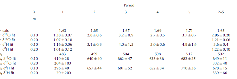
To test whether the range in fitted values of τ may be explained by the uncertainty of ρ_f , we convert the fitted values of τ into ρ_f via Equation (6). These results are shown in Table 3 and clearly suggest that the uncertainty in ρ_f of ±50 kg m⁻³ cannot explain the large differences in fitting. For example, over periods 2–5 the fitting suggests >300 kg m⁻³ difference between the lower and the upper part of the stack, which is far beyond our error limits of ρ_f .

If we then want to explain the trend in mismatch between our calculations and our measurements of ∂δ_i (t), we need to find reasons for (i) non-linear change in ρ_f with time, and (ii) a non-homogeneous change in p _f with depth. The first may be explained by the fact that densification is a function of T, and the temporal minima in T in period 2 could have influenced the development of ρ_f and τ. Further, the measured changes in the thickness of the stack at the start of the experiment show a non-linear behaviour.

The second change is more difficult to explain. It would be logical if the firn stack developed a vertical gradient due to gravity, in such a way that the stack would be denser in the lower part. This could be possible even if ρ_f was homogeneous at the start. A weak density gradient may well exist within our error bars. As discussed earlier, the positive feedback by shortening of λ is overpowering the negative feedback on ∂δ_i (t) by increasing ρ_f , explaining how the measured ∂δ_i (t) is larger than the calculated values at the bottom of the stack, despite probable increase of ρ_f . In our analysis of the compaction of the isotopic extrema, leading to Figure 4, we did not find significant evidence of larger compaction rates at the lower part of the stack, as compared to the upper part of the stack. Furthermore, ρ_f needed for the fitted values of τ using Equation (6) would range between 330 kg m^–3 for the thicker layers and 650 kg m^–3 for the thinner layers, which far exceeds the error bars on ρ_f from our measurements.

The sensitivity test shown in Table 3 is calculated with the analytic method 3. As seen in Tables 1 and 2, method 3 is the worst-performing method. The results in Table 3 would be similar using the other methods, but somewhat moderated. For example, τ δ¹⁸O fit in Table 3 for periods 2–5 calculated with method 2 is 2.06 for short wavelengths and 1.07 for long wavelengths.

We must again stress that there is a generally good fit between the calculated and the measured ∂δ_i (t), but the trend of misfit between upper and lower parts of the stack is of interest when it comes to diffusion in porous media, which may allow us to expand further upon this issue. At this point, the reasons for the misfit between the calculated and the measured ∂δ_i (t) are of course speculative, although we hope that the discussion below may help further progress in this field.

As stated earlier, on a purely physical basis the uncertainty of ρ_f can explain part of the discrepancy, but the time-trends point to more complex behaviour of the firn stack than can be explained by the simple models of densification and development of τ we have used. The general definition of τ is the ratio of the effective diffusion path through a porous medium and the length along the major diffusion axis (Reference EpsteinEpstein, 1989; Reference Champoux and AllardChampoux and Allard, 1991). In most disciplines, though, τ is simplified as an inverse function of porosity (ϕ) (e.g. Reference BoudreauBoudreau, 1996), or in some cases as permeability (Reference Pape, Tillich and HolzPape and others, 2006). Equation (6) assumes ρ_f describes ϕ, and therefore ρ_f can be used to calculate τ. This assumption is likely to be correct on a larger scale in ice columns, but empirical data have shown that firn permeability and density are not necessarily related with each other on length scales shorter than a few meters (Reference Albert and ShultzAlbert and Schultz, 2002; Reference Rick and AlbertRick and Albert, 2004). The reasons why ρ_f and ϕ ⁻¹ do not always follow each other in snow and firn are the stratigraphic history during deposition (weather) and the thermal evolution of the snow/firn pack, which produces different gradients in ρ_f and ϕ. One such example in natural snow is the formation of depth hoar, which creates a large increase in ϕ, but not necessarily a similar magnitude of decrease in ρ_f . Hence, small-scale variability in ρ_f and ϕ can have an important impact on the vapor flux, and the diffusion in snow/firn packs. Reference Kaempfer, Schneebeli and SokratovKaempfer and others (2005) managed an X-ray microtomography of a snowpack made of sieved naturally formed ice crystals, and found that τ was more dependent than ρ_f on the geometry of the ice matrix. This supports the assumption in Equation (6) that states τ = f(ρ_f ⁻¹) is an oversimplification, at least on length scales smaller than a few meters. An analogue conclusion was made by Reference Tuli, Hopmans and RolstonTuli and others (2005) who studied the change in permeability in soil packs before and after repacking the soil. They found that the permeability changed after the repacking of the soil, despite the fact that both ρ and ϕ were held constant between the two packings of the soils. Their conclusion was that the texture of the grains and their orientation (fabric) was an important factor in the determination of τ.

This short review of the current perspective of τ in porous media clearly shows that τ = f(ρ_f ⁻¹) is an oversimplification. In natural snow/firn packs, a considerable short-frequency variation in the depth distribution of ρ_f and ϕ exists. The fabric and geometry of the ice grains, and hence τ, may be one of the key unknowns that trigger instability in back-diffusion calculations (e.g. Reference Bolzan and PohjolaBolzan and Pohjola, 2000; Reference Johnsen, Clausen, Cuffey, Hoffmann and SchwanderJohnsen and others, 2000). Equation (6) assumes that the low-frequency distribution of ρ_f determines τ and therefore controls ∂δ_i (t). The short-frequency distribution of ρ_f, ϕ, fabric and geometry of the ice grains may have a larger impact on ∂δ_i (t), than the low frequency value of ρ_f indicates.

An illustration of the complexity of vapor diffusion in the short-frequency domain was shown by Reference Sokratov and MaenoSokratov and Maeno (2000), who studied the development of the vapor diffusion coefficient in snow forced by a temperature gradient. They created a constant temperature gradient over the snowpack and thus controlled the thermally driven vapor diffusion. However, even as they strove hard to keep all parameters constant along the snow profile, the temperature distribution varied with a wave-like pattern within the snowpack. These temperature waves inflicted changes in the snowpack, and changed the properties ρ_f, ϕ and τ, which made Sokratov and Maeno introduce an enhancement factor in their diffusion equation. Whether the change in the properties was an effect of the thermal flux or an effect of an already existing inhomogeneity in their experiment is not known, but the temperature distribution and the change of the properties clearly operated together in a positive feedback loop. This shows that small-scale inhomogeneities can bring forward substantial changes of the ice properties via feedback loops, and in order to get better generalizations of macro-processes of vapor diffusion in firn we have to study micro-processes more closely.

How can the results referred to above be used to explain the lack of exact match between calculated and measured ∂δ_i (t) in our experiment? First, we find that the possibly inadequate parameterization of τ in Equation (6) is a likely candidate of our misfit. We have already rejected ρ_f differences between the top and bottom layers as the dominant operator for the misfit, and, based on the same observational arguments, ϕ is also not a likely candidate. The textural properties, such as grain size and fabric, may, however, be a control of τ in our experiment. Our initial plan was to have the grain distribution as homogeneous as possible in our experiment, and we observed no obvious signs of difference in sorting between the upper and lower layers of the stack. Either the fabric in the lower part of the stack became more aligned compared to the upper layers due to the packing, resulting in decreased τ in the lower and thicker layers, or some post-‘depositional’ processes operated so that grain sizes changed differently between the lower and the upper parts of the stack.

One possibility could be a relatively larger growth rate of crystals in the lower part compared to the upper part, where for geometrical reasons larger crystals would have larger pore spaces, and therefore lower τ. The densification, or sintering in the experiment, was rather large. This may be due to the instant densification discussed earlier, or to the high specific area of the artificially produced ice flakes, which promotes greater sintering than the more spherical grains that occur in natural firn packs.

Another possibility for the difference in τ between the lower and the upper parts of the firn stack is that we have a preferred recrystallization of new crystals in the upper part compared to the lower part of the stack. Re-nucleation usually starts with small grains, and Reference Pape, Tillich and HolzPape and others (2006) have shown that an increase in the fractal dimension of grains increases τ. As a result, if we have some gradient that drives vapor from the lower part of the stack towards the upper part of the stack, recrystallization may increase the fractal dimension of grains in the upper part of the stack compared to the lower part. As shown earlier, our experiment was sited in a well-insulated box, and we discard any gradients within the box that could drive such processes.

The experiments by Reference BraudBraud and others (2005) concerning diffusion in partly wetted soils also found that the δ²H/δ¹⁸O relationship changed to a larger degree than could be explained by molecular diffusion. They had no advection of air in their experiment, but they suggested that the wetting front experienced turbulent diffusion due to evaporation, and created this fractionation. Since the fractionation rates are different for δ²H and δ¹⁸O, this produces a change in the δ²H/δ¹⁸O relationship with time. Their experiment had a different set-up than our firn experiment, but both these experiments showed the unexpected change of the δ²H/ δ¹⁸O relationship. As shown in the Results section, ∂δ_D (t) was found to be higher than expected in our experiments, while ∂δ¹⁸O(t) were more similar between calculated and measured values (at least for the more stable method 2). The question, then, is whether or not in our experiment there was fractionation through a sublimation/recrystallization cycle with a related change in the δ²H/δ¹⁸O relationship. If we had a measurable amount of recrystallization through sublimation, then the δ²H/δ¹⁸O relationship should change with time. Figure 6 shows the δ²H/δ¹⁸O relation for the measured isotopic profiles during periods 1 and 5, as well as the forward-calculated isotopic profiles from period 1 to 5. The linear regressions of all three relations were 5.4 ±0.1, suggesting no fractionation was present, which argues against any notable effect of different rates of recrystallization between the upper and lower parts of the stack. Hence the question why the difference between modelled and measured values is higher for ∂δ_D (t) than ∂δ¹⁸O(t) remains unanswered.

Fig. 6.

Co-isotopic plots of the measured isotopic distributions in period 1 (crosses) and period 5 (triangles) and the forward-calculated distribution in period 5 using method 1 (dots).

Conclusions

In this experiment we build an artificial firn stack, in order to monitor and measure vapor-driven diffusion of water isotopes with time. We then compare the measurements with calculations of diffusion rates from a theoretical- and empirical-based model of vapor-driven diffusion in firn. We use three different methods in our analysis, including a new analytic method based on an input function composed of a Fourier series of harmonic functions, and find that all methods give similar output, but also that each method has its own pros and cons.

We find a generally good agreement between calculated and measured diffusion rates of δ¹⁸O and δ²H, which confirms the state-of-the-art knowledge of diffusion of isotopomers in unventilated firn, as described by Reference Johnsen, Clausen, Cuffey, Hoffmann and SchwanderJohnsen and others (2000). A detailed study, however, shows >13% higher diffusion rates of the thicker layers, and <8% lower diffusion rates of the thinner layers than theory predicts, leading us to conclude that our calculations with the state-of-the-art theory under-predict the diffusion rates in thicker layers, and over-predict the diffusion rates in thinner layers.

The firn had different average temperatures during the studied periods, and we find that the modelled diffusion rates compare well with measured values, and thus the current theory reflects changes in firn temperature well. The largest uncertainty in our experiment was the firn density, where a 10% uncertainty of the firn density leads to up to 30–40% difference in the calculated diffusion rate. This leads us to conclude that precise control of firn density and grain geometry in the firn stack is important in future experiments of a similar kind. We further test whether recrystallization due to sublimation has been an important process in our experiment, but find that no such fractionation can be detected from the co-isotopic ratios, and we have no evidence to infer recrystallization as an important process here.

We finally suggest that the tortuosity of the firn is the crucial, unknown parameter in this work. The fitting procedure shows that we have to change the tortuosity parameter beyond the uncertainty in the firn density in order to match modeled results to observations. This in turn suggests tortuosity is partly related to factors other than firn density alone. In order to improve similar experiments in the future, we recommend the measurement and monitoring of changes in the size of the firn grains and their fabric in the firn stack, which likely are important parameters controlling the tortuosity of the vapor flux. The uncertainty in the likely short-scale spatial and temporal variability of tortuosity may also partly explain instability in the inversion of the firn diffusion equation as applied to ice-core records.