Introduction

The mass balance and stability of the West Antarctic ice sheet are, in large part, determined by the dynamics of the large ice streams that drain it. The ice streams of the Siple Coast are the most extensively studied, and it has been found that they can undergo significant changes over relatively short time-scales of l00 years or less. The rapid motion of Ice Stream C stopped some 100 years ago (e.g. Reference Alley and Whillans.Alley and Whillans, 1991), and there have been significant changes on Ice Stream D in the past few centuries (Reference Hodge and Doppelhammer.Hodge and Doppelhammer, 1996). Significant changes have also occurred on Ice Stream B (Reference Alley and Whillans.Alley and Whillans, 1991; Reference Clarke and Bentley.Clarke and Bentley 1995). More recent changes in the width and speed of Ice Stream B have been documented by Reference Bindschadler and Vornberger.Bindschadler and Vornberger (1998); they were both rapid and of large magnitude.

It has been shown that the margins of at least some ice streams play an important role in ice-stream dynamics by supporting much of the downslope load (Reference Echelmeyer, Harrison., Larsen. and Mitchell.Echelmeyer and others, 1994; Reference Scambos, Echelmeyer., Fahnestock. and Bindschadler.Scambos and others, 1994; Reference Jackson and Kamb.Jackson and Kamb, 1997; Reference Whillans and van der Veen.Whillans and Van der Veen, 1997; Reference Harrison, Echelmeyer. and Larsen.Harrison and others, 1998). The thermomechanical stability and migration of these margins, and thus of the width of an ice stream, has been discussed theoretically by Jacobsen and Raymond (1998). They find that the width of an ice stream is likely to vary at rates of one to a few tens of m a⁻¹. Such width variations are directly coupled to the mass balance of the ice sheet through the ice-drainage flux, and specific knowledge of ongoing changes is necessary as input to any calculation of the present balance.

The position of the shear margin of an ice stream is reasonably well defined on a large scale, such as in satellite or aerial photographs. However, resolution of the “true” margin in these images is probably limited to about 100–300 m, which is insufficient for determining migration rates over short time-scales. Similarly, detailed field mapping of crevasses at the edge of the marginal zone is limited by-changes in surface snow cover and by ambiguities in defining specific crevasses and their length; this method probably has a resolution of about 100 m. Reference Hamilton, Whillans. and Morgan.Hamilton and others (1998) have used a somewhat more accurate method, involving crevasse curvature, to determine the rate of margin migration on Ice Stream B; they find an outward rate of 7–30 m a⁻¹.

We have presented an indirect method for determining the outward migration of one margin of Ice Stream B. That method was based on the diffusion of cold winter temperatures into the ice beneath the heavily crevassed shear margin (Reference Harrison, Echelmeyer. and Larsen.Harrison and others, 1998), and it indicated that the margin at this location was moving outward into the ice sheet (the “Unicorn”, Fig. 1) at an average rate of about 7.3 ± 1.5 m a⁻¹ over the last half-century. This rate of outward migration is similar to that of Reference Hamilton, Whillans. and Morgan.Hamilton and others (1998), but it is in the opposite direction and slower than the migration at the same location sometime in the past century or two as estimated by Reference Clarke and Bentley.Clarke and Bentley (1995).

Fig. 1.

Map showing location of profile and various sites listed in Table 1. Modified from Vernberger and Whillans (1986) and Reference Shabtaie and Bentley.Shabtaie and Bentley (1988).

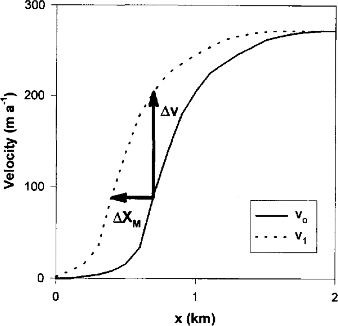
In this paper we present a method for directly measuring the ongoing migration of an ice-stream margin. The basic concept of this technique is that, as the ice-stream margin moves sideways, there is a concomitant lateral shift in its characteristic velocity profile (Fig. 2). This velocity profile is one of the “signatures” of ice-stream flow, with an abrupt increase from the slow ice-sheet regime to the fast flow of the ice stream, and the position of the peak transverse velocity-gradient “marks” the edge of the ice stream. Because of this large velocity gradient, outward migration of the margin would cause apparent accelerations at spatially- fixed transverse positions along the profile, and any two consecutive measurements of the velocity profile could be used to determine the lateral migration of the shear margin, as shown schematically in Figure 2. In this method we thus take the shape of the velocity profile to be defined in a Lagrangian sense with respect to the ice-stream margin: it is not fixed in space. We also require that the ice-stream velocity be relatively steady in time, as we are interpreting local accelerations as being caused by a lateral shift in the margin.

This method is applied to velocity data from the same location on Ice Stream B as discussed by Reference Harrison, Echelmeyer. and Larsen.Harrison and others (1998). The resulting migration velocity is in good agreement with the value they determined. We also present detailed ice-thickness measurements through the marginal zone of the ice stream, as these are needed to check the validity of one of our central assumptions in this analysis. These depths will also prove useful for detailed force-balance and flow modeling of this ice stream.

Fig. 2.

Schematic drawing of the longitudinal surface velocity across an ice-stream margin at two times(v₀ and v₁). A shift ΔX_M in the profile gives an apparent change in velocity Δν at a fixed position x.

Setting and Measurements

We seek to determine the present speed of migration of the ice-stream margin relative to a fixed (geographic) coordinate system, and in the following we define “inward” to be in the direction from the slow-moving inland ice, which we call the “ice-sheet” flow regime, into the ice stream, and “outward” to be from the ice stream to the ice sheet. In our example, we focus on Ice Stream B2 in the vicinity of Upstream B camp (UpB). The “ice sheet” in this region (i.e. the slower-moving “inland ice”) is the Unicorn, which is actually a peninsula (or island) of the inland ice of West Antarctica (Fig. 1). This feature is bordered on the south by Ice Stream B1 and on the north by B2, and these two streams coalesce at its lower end. The Unicorn is not a large-scale feature like ridge BC or Siple Dome (Fig. 1).

The marginal shear zone of Ice Stream B2 at this location (the “Dragon”) consists of three distinct sub-zones. These is an outer zone of large arcuate crevasses some. 400 m long, followed by a 2 km wide zone of chaotic crevassing. The transition between these two zones is diffuse, and fully chaotic conditions exist only inward of the first 150 m or so of the second zone (Fig. 3). The innermost sub-zone consists of somewhat organized and widely spaced “shear” crevassing; it is also about 2 km wide. The complete transverse profile of surface velocity from the Unicorn, across the Dragon and extending to the center of the ice stream has been discussed in detail by Reference Whillans and van der Veen.Whillans and others (1993) and Echelmeyer and others (1991). The longitudinal velocity shows a marked increase from 2 m a⁻¹ on the Unicorn to about 430 m a⁻¹ near the center of the ice stream, with most of the increase occurring within the shear margin itself. Maximum transverse shear strain rates are about 0.7 a⁻¹, and they are localized within the zone of chaotic crevassing.

Fig. 3.

Map of marker locations relative to the structure of the margin and the fixed coordinate system. Open circles are boreholes discussed by Reference Jackson and Kamb.Jackson and Kamb (1997) and Reference Harrison, Echelmeyer. and Larsen.Harrison and others (1998): C, Chaos; LL, Lost Love; D, Dragon Pad; ST, Stage. Azimuth of they axis is S77°W ( True), which is equal to the azimuth of the local margin.

Here we focus on a limited section of the marginal zone extending from within the Unicorn to about 1.8 km into the Dragon, denoted the “S” profile (Figs 1 and 3). This limited profile, with total length about 2.5 km, traverses across the arcuate crevasses and into, but not across, the chaotic sub-zone. The sampling borehole of Reference Jackson and Kamb.Jackson and Kamb (1997) and four of the boreholes discussed by Reference Harrison, Echelmeyer. and Larsen.Harrison and others (1998) are located along the S line, as indicated in Figure 3.

In December 1993, 20 marker poles were placed in the firn at locations spaced about every 100 m across this transverse section by a roped field party traveling on skis. Retro-reflecting prisms were mounted on most of the poles, so that future surveys would not require reoccupation. The markers were surveyed from a base station (S17) using a 1 s theodolite and an accurate (±2 mm + 1 ppm) electronic distance meter. Surveys of the complete profile were performed on 6 December 1993, 18 January 1994 and 17 January 1995. These dates define two epochs, Δt ₀ and Δt ₁, over which the velocity was calculated. These two velocities (v ₀ and v ₁) are the mean velocities over these time intervals, and, assuming that the velocity is constant over each epoch, they apply at the mid-times t ₀ and t ₁, where

and where time zero is taken to be 0000 h on 1 January 1994.

Additional markers were placed up- and downstream of the transverse profile at selected locations (Fig. 3) for evaluation of the surface strain-rate field about the profile. The backsight for all surveys was located at marker 121 (station 21 of Reference Whillans and van der Veen.Whillans and Van der Veen (1993) and station DG37 of Reference Hamilton, Whillans. and Morgan.Hamilton and others (1998)).

Absolute velocity of base station; orientation of the margin and profile

Our method requires the absolute velocity of the ice. To accomplish this, we used geodetic global positioning system (GPS) methods to determine the absolute positions of our base station and backsight. To minimize the errors in this absolute velocity determination, we established a fixed benchmark on the closest bedrock to our survey site, which was a nunatak on the Ross Ice Shelf near the mouth of Leverett Glacier, 204 km to the south (Fig. 1). Dual-frequency GPS receivers were run simultaneously at the sites for about 6 hours in January 1994 and again in 1995. The azimuth of the baseline from S17 to 121 was also determined during each of these two surveys, as well as a third time using static GPS methods between the two points. These three measurements enable us to quantify the rotation rate of the profile accurately.

The long-baseline GPS data were processed by M. Chin of the U.S. National Geodetic Survey using precise orbits. The estimated accuracy of the solution was a few tenths of a ppm, or about 0.06 m for our relatively short 204 km baseline. This leads to an estimated error of 0.1 m a⁻¹ for the absolute velocity of the base station. The velocity of the backsight relative to S17 has a better accuracy because of the short distance involved; it is about 0.01 m a⁻¹. As shown in Table 1, the base station is moving at about 3 m a⁻¹, directed into the ice stream at an angle of about 26° to the margin. The backsight 121 is moving in at a somewhat steeper angle, but slightly slower because it is a few hundred meters further away from the effects of ice-stream drag.

Table 1.

Coordinates and velocities of selected stations shown in Figure 1

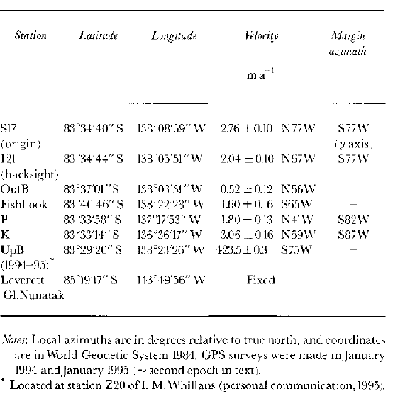
Velocities of a few other points on the Unicorn and at the 1994–95 location of UpB (Fig. 1) were also determined using static GPS methods from 121 in 1994 and 1995; they are shown in Figure 1 and listed in Table 1. The associated errors are dominated by the error in the absolute velocity of 121. All of the points on the Unicorn are moving slowly, with speeds which indicate an ice-sheet flow regime, supporting our assumption that the Unicorn is part of the inland ice.

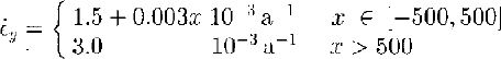
The 1994–95 speed at UpB is 423 m a⁻¹. This is 4% lower than the speed measured at this station in 1984–85 by Reference Whillans, Jackson. and Tseng.Whillans and Van der Veen (1993). However, the physical station was 4 km upstream at the time of their survey. The longitudinal velocity gradients of Reference Hulbe and Whillans.Hulbe and Whillans (1997) indicate that this part of the ice stream has a longitudinal extension of somewhat more than 10⁻³ a⁻¹, and therefore the 1994–95 speed at the 1984–85 position would actually be about 420 m a⁻¹. This observation of a 22 m a⁻¹ decrease in speed at UpB agrees well with that of Reference Hulbe and Whillans.Hulbe and Whillans (1997) for the period 1984–85 to 1991–92, and indicates a continuing slowdown of this part of the ice stream. The effect of this slowdown on our analysis of margin migration is discussed below.

The velocities listed in Table 1 can be compared with those at nearby locations given by Reference Whillans and van der Veen.Whillans and Van der Veen (1993) and Reference Hamilton, Whillans. and Morgan.Hamilton and others (1998). At 121, Reference Whillans and van der Veen.Whillans and Van der Veen (1993) found a speed of 1.5 ± 0.5 m a⁻¹, while Hamilton and others found 1.98 ± 0.02 m a⁻¹. Our site Fishhook is close to station 72 of Whillans and Van der Veen, where they found a speed of 1.7 ± 0.5 m a⁻¹, and our site K is close to their station 71, where they measured 2.9 ± 0.5 m a⁻¹. The agreement between their speeds and ours (see Table 1) is good at all these locations.

GPS methods were also used to determine the orientation of the shear margin. The positions of the margin at the S profile and on lines located about 5 km upstream and 5 km downstream of S were determined by skiing from the Unicorn through the arcuate crevasses and about 150 m or so beyond, passing through a region of heavy but not yet fully chaotic crevassing. The party continued until all four members agreed that the crevassing had become “fully chaotic”. A static GPS measurement was then made relative to our base station. Full chaos occurred at S9 along the S profile. While this method was somewhat subjective, we found that the transition to fully chaotic conditions could be identified reliably to within about ±20 m. The margin has a slight curvature along the Unicorn, as is shown on the maps of Reference Vornberger and Whillans.Vornberger and Whillans (1986). We used our three measurements to constrain this curvature (0.4° km⁻¹) and its local tangent to about ±0.2°. The local tangent we term the “azimuth of the margin” at S (Table 1). Similar measurements were made near P and K (Fig. 1; Table 1).

We take the y axis to be parallel to the azimuth of the margin and directed approximately along flow. x is taken to be normal to this margin and directed into the ice stream from the Unicorn (approximately north), and z is vertically upward. The origin is defined to be the position of the base station (S17) at the time of the first survey. Explicit information regarding the coordinate system is given in Table 1 and Figure 3. Because our base station moved and the baseline to the backsight rotated relative to the fixed y axis, we defined a local coordinate system on each of the survey dates, and then applied a rotation and a translation to these coordinates to place them in our fixed system. Our GPS surveys indicate that the rotation rate of the backsight baseline was constant over the survey period, so we made a linear interpolation of the azimuth to the dates of our profile surveys. We also assumed that the velocity of S17 was constant, thus enabling a linear interpolation of its translation.

Velocity Along the S Profile

The components of velocity for each marker were calculated for the two epochs; they are shown in Figure 4a and b. Propagation of errors in the angle measurements (±2^″), the distances (±0.004 m) and tilt of the poles (±0.01 m for t ₀ and ±0.02–0.04 m for Δt ₁, depending on the surface conditions at each marker) gives an estimated accuracy for the velocities of the different markers relative to S17 of 0.15–0.22 and 0.05–0.08 m a¹ for Δt ₀ and Δt ₁, respectively. Including the errors in the absolute velocity of S17 leads to estimated errors of about 0.20 and 0.12 m a⁻¹ in the absolute velocities over the two time periods. Neither of these two error estimates includes a contribution due to errors in the azimuth of the baseline; these are discussed separately below.

Fig. 4.

(a) Longitudinal component (v_y) and (b) transverse component (v_x) of surface velocity across the S profile. v_y is shown for both epochs (Δt₀ and Δt₁), while v_x is shown only for the longer epoch, Δt₁. The inset in (a) shows an enlargement of the two longitudinal velocity curves, with the curve from Δt₀ being below that from Δt₁.

In general, the longitudinal velocity, v _y, is large relative to these errors, and the pattern shown in Figure 4a appears to be relatively smooth. Except for the markers on the Unicorn (stake numbers ≥S15), the transverse component, v _x, is much smaller than v _y (Fig. 4b). On the Unicorn there is only a small increase in v _y as the margin is approached, but once the arcuate crevasses are entered (near S15) the speed rapidly increases. In this sense the shear margin of the ice stream begins at about S15.

The markers near S17 move into the ice stream at about 1 m a⁻¹. Inward of this, the pattern of transverse velocity is determined by departures of the profile layout from linearity along the x axis (Fig. 4b): slight offsets of the markers up-and down-glacier from the x axis (Fig. 3) give rise to small positive or negative transverse-flow components, respectively. In part, this is due to the curvature of the margin (0.40° km⁻¹) about our fixed x axis.

Strain Rates

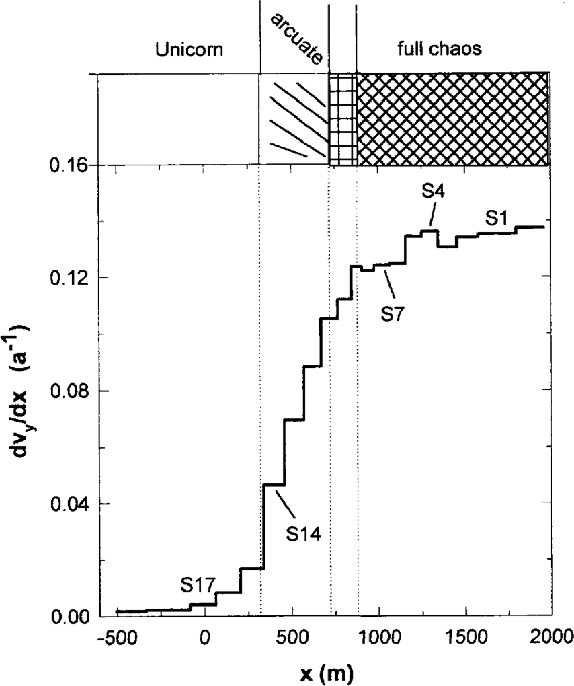
The velocity gradient ∂v _y/∂x is shown in Figure 5. Our measurements show that the other gradient, ∂v _x/∂y, is small in this region (~0.001 a¹), so the value shown in Figure 5 is approximately twice the shear strain rate, έ _xy. The accuracy of ∂v _y/∂x is about 0.001 a⁻¹. Arcuate crevassing extends from S15 to about S11, where ∂v _y/∂x rapidly increases from 0.02 to about 0.10 a⁻¹. Fully chaotic conditions exist where ∂v _y/∂x is in the range 0.12–0.14 a⁻¹.

Fig. 5.

Histogram showing the transverse gradient of the longitudinal velocity, ∂v_y/∂x.

In the rest of this analysis we consider only the longitudinal component of flow. Unless needed for clarity, we omit the “y” subscript (v ≡ v _y).

Because we did not reset our markers to their original positions between the two velocity surveys, the velocity of a marker is subject to spatial changes in the velocity field. It is necessary to correct for these changes before an accurate comparison of v ₀ and v ₁ at a fixed position can be made; this requires the horizontal strain-rate field.

The markers that were placed up- and downstream of the S profile (Fig. 3) define three “diamonds” within which we can calculate the horizontal components of the strain-rate tensor. Each of the diamonds had major axes of about 1 km, or one ice thickness. Diamond I was centered about the origin, which is on the uncrevassed Unicorn; II was centered at x ~500 m within the arcuate crevasses; and III was centered at x ~1400 m within the fully chaotic zone. They were each surveyed three times.

The diamonds were not oriented precisely along the coordinate axes, nor were they composed of strict right angles between equal-length sides. To account for this we calculated the average rate of elongation (i.e. the normal strain-rate component) along each major axis and along each pair of sub-parallel sides within the figures. Along the sides, two each oriented at nominal angles of 45° and 135° to the x axis, we averaged the elongation rate of the two sub-paralell sides, and also determined their mean angle θ with respect to x. The elongation rate over time Δt of a line segment with original length l ₀ and final length l ₁ is

(1)

Tensor component rotation then gives an expression for each of the four average έ _θ‘s in terms of the three horizontal strain-rate components (έ _x, έ _y, έ _xy) in the x, y-coordinate system defined above. These four relations were solved for the three unknown strain-r ate components using normal equations (Reference SchigolevSchigolev, 1965). The resulting strain rates are strictly applicable to the centroid of each diamond; these centroids were close to the x axis. Strain rates were measured over both Δt ₀ and Δt ₁, and they were found to be similar; this is probably because the markers did not move appreciably relative to the size of the diamonds. The accuracy of the normal strain-rate components is about 0.5 × 10⁻³ a⁻¹.

The results of these measurements show that within the Dragon έ _y and έ _x are relatively constant at 3.0 × 10³ a¹ and –1.5 × 10⁻³ a⁻¹, respectively. Their magnitudes decrease to zero within the Unicorn. These are similar to the values found by Reference Whillans and van der Veen.Whillans and others (1993) in the same region using repeat aerial photogrammetry. In a later section we require ε _y as part of a correction to v ₁ (x); for this we use the following fit to our measured values (x in m):

(2)

The shear strain rates determined from these measurements agree well with one-half the gradient shown in Figure 5, again because ∂v _x/∂y is small. The principal horizontal strain rates, which are often used in the analysis of crevassing, are oriented at about 45° to the x axis, and their magnitudes are approximately equal to (1/2) ∂v _y/∂x because the normal strain rates are so small. Thus the relation between the magnitude of the transverse velocity gradient shown in Figure 5 and the arcuate and chaotic zones that was discussed above holds for these principal strain rates as well.

Ice Thickness

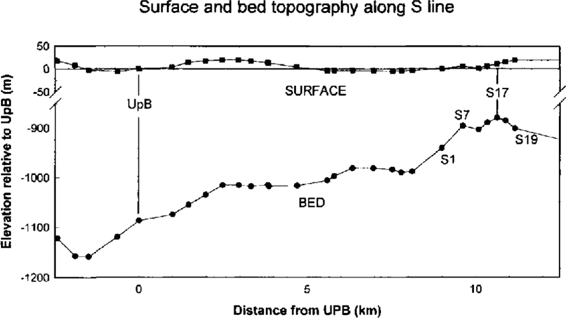
Lateral changes in ice thickness are important in determining the velocity field of valley glaciers, and our modeling shows that such changes can affect the fine structure of an ice stream’s velocity field, in particular the shape of the velocity profile that we have assumed is fixed. Airborne ice-radar soundings of Reference Shabtaie and Bentley.Shabtaie and Bentley (1988) and Reference Retzlaff, Lord. and Bentley.Retzlaff and others (1993) indicate that the thickness of Ice Stream B varies by 200 m or so across the ice stream near UpB. However, the necessarily large scale of their surveys and presentations makes it difficult to define the fine-scale structure of the marginal zone, which we require. To this end we made ground-based monopulse radar measurements along the S transect, continuing on to the center of the ice stream. The results (Fig. 6) indicate that at this location the ice stream fills a shallow trough that is 300 m, or 30%, deeper near the center than at the southern margin. Beneath the arcuate and chaotically crevassed zones (~2.5 km wide) the thickness varies by about 120 m. It is important to take these thickness variations into account when calculating force balances (e.g. Reference Jackson and Kamb.Jackson and Kamb, 1997; Reference Harrison, Echelmeyer. and Larsen.Harrison and others, 1998) or modeling the details of ice-stream flow, and they will be used in our analysis below.

Fig. 6.

Surface and bed topography across Ice Stream B2 along an extension of the Sprofile through UpB. Errors in ice depth are about ±30 m and those in surface elevation are ±1 m relative to UpB. (Elevation of UpB is approximately 360 m above the ellipsoid.) Vertical exaggeration is 15:1.

Velocity Difference Between the Two Epochs

Velocities for both epochs are shown in Figure 4a. There appear to be slight differences between the two curves; these are amplified in the inset figure. At most locations the later velocities (v ₁) are larger than the earlier ones (v ₀), which is what we would expect if the margin is moving outward.

Difference in Velocity

The uncorrected difference between these two velocities,δν ≡ v ₁ – v ₀, is shown in Figure 7. The difference is small within the Unicorn, and increases to about 0.8 m a⁻¹ near S11 to S8. Inward of this, corresponding to the fully chaotic zone, there is significant scatter in δν. These velocity differences are to be compared with the estimated errors in δν, which are about 0.15–0.23 m a¹, depending on location. The differences in the transverse velocities (v _x) are small (< ±0.2 m a¹) and scattered about zero.

Fig. 7.

Uncorrected (δν ≡ v₁ – v₀) and corrected (Δν, Equation (5) ) difference in longitudinal velocity between the two epochs.

To check for the effects of any misalignment of x relative to the normal of the shear margin, we rotated the coordinate system by ±10° and recalculated δν. The results are nearly identical to those in Figure 7, and thus we are assured that the magnitude of δν does not depend on our choice of coordinate axes.

Correction of Velocity Difference for Non-Zero Strain Rates

The two velocities v ₀ and v ₁ are spatial averages over two different regions of the surface. We assume that the position at which each of these velocities applies is the midpoint of the line segment between the two points surveyed at the beginning and end of each epoch. This effectively assumes that the velocity was constant over each epoch, and that the strain rates are constant along the displacement vectors, as supported by our measurements.

The midpoints of each marker’s path during Δt ₀ and Δt ₁ are at different locations within the velocity field, and before the velocity difference between the two epochs can be used as an accurate measure of margin migration we must correct for along-path velocity gradients. We take the velocity v ₀ to be the base value for comparison, and thus need only correct v ₁. The midpoint of the second epoch, at which v ₁ applies, is displaced by components (Δx _mid, Δy _mid) from the midpoint of the first epoch, each of these components being equal to the sum of one-half the displacement over Δt ₀ plus one-half that over Δt ₁:

(3)

Two corrections to v₁ are necessary: one for longitudinal and one for transverse motion in the velop>city field. The corrected velocity difference, Δv, is:

(4)

where έ _y is obtained from Equation (2) and ∂v _y/∂x from Figure 5. The correction for motion along x is generally in the range ±0.07 m a¹, while along y it is about 0.01–0.33 m a⁻¹ depending on the position within the shear margin. This corrected velocity difference is also shown in Figure 7, where we see that the corrections do not alter the patterns in the velocity difference, nor do they significantly affect its magnitude. In particular, the scatter in Δv inward of S8 remains.

Calculation of Migration Velocity

As shown in Figure 2, an outward shift ΔX _M(< 0) in the velocity profile with respect to the markers causes an apparent velocity increase Δv at each marker. The magnitude of Δv is governed by the local shape of the profile, or ∂v _y/∂x:

(5)

This shift is assumed to occur at a uniform rate V_M over a time interval Δτ ≡ t ₁ –t ₀ = 203.518 d. (Strictly speaking, Δτ Should be the difference between the times at which the midpoints of the two displacement vectors are reached, but because the strain rates are nearly constant and because the correction terms in Equation (4) are small, these times very nearly correspond to the mid-times of the two epochs.) Then, allowing for a change in sign so that outward migration is positive, ΔX _M = –V _MΔτ, or

(6)

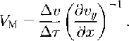
We have calculated the apparent migration rate from Equation (6) using the data shown in Figures 5 and 7. The results are shown in Figure 8. V _M is positive almost everywhere, implying that the margin is indeed migrating outward. The rate is nearly uniform from S15 to about S6, with a mean of 9.7 m a⁻¹ and a standard deviation of 1.7 m a⁻¹. Inward of about S6 the calculated migration rate is erratic. It is also erratic at points located within the Unicorn; because of the large errors involved, as described next, these values are not shown.

Fig. 8.

Calculated margin migration rate, V_M. Error bars were calculated using Equation (7). Dashed line is the average value for S15 to S6.

Errors in Calculated Migration Rate

The error in V _M, denoted σV_M, is given by

(7)

where σ _Δv is the estimated error in the corrected velocity difference and σ _∂v/∂x is the error in the velocity gradient (≈1 × 10⁻³ a⁻¹). In most cases, the error in the corrected velocity difference is dominated by the error in the first epoch’s velocity (0.15–0.23 m a⁻¹) because the short time interval (0.12 a) amplifies the surveying errors. Errors in the correction terms (Equation (4)) are small, and those in v _l (relative to S17) are about 0.05-0.08 m a⁻¹.

There is one additional source of error in Δv that must be considered, that due to uncertainty in the rotation of the baseline. As mentioned earlier, the vector from our survey-base (S17) to the backsite (I21) was surveyed using geodetic GPS methods. Three such surveys indicate that the baseline was rotating at a constant rate, and this rotation was accounted for in the calculations. If, however, the rotation between two surveys was in error then this would introduce a systematic error in all coordinates calculated using that baseline. In particular, if there were an error of 16″ in the baseline azimuth at the intermediate survey or about 130″ in that of the final survey, then the calculated migration rates would be indistinguishable from zero.

We have investigated possible error sources in this baseline azimuth, including instrument centering, pole tilts, the GPS solutions and the optical surveys to the backsight. The combined uncertainty is about 5″, which is much less than the limiting values stated above. Combining all the possible error contributions gives σ _Δv = 0.15–0.27 m a¹, depending on the distance from S17.

Equation (7) shows that when the velocity difference and/or the velocity gradient are small then the error in the migration rate will be large. These conditions occur at markers situated on the Unicorn (S19–S16; see Figs 5 and 7), and at these locations the estimated errors are ≥40 m a^l! The results from these slow-moving sites are thus highly inaccurate, and we therefore consider only those at S15 and inward. The estimated errors, including a possible systematic error in the baseline azimuth, are shown by the error bars in Figure 8. Inward of about S14 (from within the arcuate crevasses into the chaotic zone) the errors are on the order of 3.5 m a⁻¹; these are smaller than the calculated migration rates.

Discussion

The results of our measurements indicate that the margin is migrating outward into the Unicorn at about 9.7 ± 1.1 m a⁻¹, where we have taken the average rate from S15 to S6 and estimated the standard error as the typical error in V _M (~3.5 m a⁻¹, which includes a possible systematic error in the baseline azimuth) divided by , where n is the number of points from S15 to S6.

Two of the key assumptions in our analysis are that the velocity profile is a characteristic feature that is transported with the margin, and that there has been no temporal change in the overall speed of the ice stream during the period of measurement. That the shape of the velocity profile was nearly identical between the two surveys and that the profile did not move far (either laterally or longitudinally) relative to the scale of the margin gives support to the validity of the first assumption. That the calculated migration velocity was approximately constant over much of the profile also supports this analysis.

The validity of the first assumption also depends on the basal topography of the marginal zone, and the associated ice thickness. It is likely that the velocity profile would reflect any abrupt steps in ice thickness that occur within the marginal zone, such as those found near the wall of a U-shaped valley glacier. A lateral shift in the margin relative to this rough basal topography would cause a change in the shape of the velocity profile. Ice thickness does change across the Dragon (Fig. 6), but maximum side slopes of the bed are on the order of 1.5° or less. Thus, significant changes in thickness occur only over 400 m or so, which is much broader than the distance over which the margin moved during our study. Thus our interpretation is unlikely to be affected by these variations in thickness.

There is an increased scatter in the measured Δv’s and the calculated migration rates inward of S6 (Figs 7 and 8). These markers are well within the zone of fully chaotic crevassing. Here the crevasse blocks on which the markers were situated are relatively small and they may rotate somewhat independently of their neighbors. However, the increased scatter may also be due in part to a failure of our assumption of a constant velocity structure within the margin. As the margin migrates laterally, the physical properties of the ice that it encounters, and its history of deformation and crevassing, may vary locally. Something similar was noted in our study of borehole temperatures (Reference Harrison, Echelmeyer. and Larsen.Harrison and others, 1998). In that case the interpretation of the data from a borehole near S1 (Fig. 3) was much less well constrained than that from the borehole at S7. Both of these studies seem to indicate that conditions are not static within the fully chaotic zone of the shear margin, which is not surprising given the nature of the surface. They may also indicate that conditions within the arcuate crevasses and the zone of transition to full chaos are more nearly constant.

The assumption of no temporal variations in ice-stream velocity has been addressed by Reference McDonald and Whillans.McDonald and Whillans (1992), Reference Harrison, Echelmeyer. and Engelhardt.Harrison and others (1993), Reference Hulbe and Whillans.Hulbe and Whillans (1997) and our recent GPS measurements. The first two studies showed that there are no large variations in the speed of this ice stream over seasonal or shorter time-scales. However, our recent measurements, and those of Hulbe and Whillans, indicate that the ice stream near UpB, 11 km inward of the Unicorn and of S17 (Fig. 1), has, in fact, slowed since 1984–85. Reference Bindschadler and Vornberger.Bindschadler and Vornberger (1998) have also observed a recent and dramatic slowdown of nearly 50% over 30 years near the mouth of Ice Stream B, some 300 km downstream.

Our measurements, together with those of Reference Hulbe and Whillans.Hulbe and Whillans (1997), suggest that the deceleration has been constant at about 0.5% a⁻¹, and we could expect a decrease over Δτ of about 1.1 ma¹ at UpB. If this slowdown were affecting the entire ice stream, then we would expect to see a deceleration across our profile, the magnitude of which decreases towards the Unicorn. As an example, if we assume a simple power-law velocity profile (u α width⁴), then S2 and S10 would have slowed during Δτ by about 0.33 and 0.11 m a¹, respectively.

Imposing such a decrease in speed across our profile would increase the calculated outward migration rate, as it would require the corrected velocity difference to be correspondingly larger to account for the slowdown. The apparent migration rates would be then be increased by about 2–7 m a¹. However, because of the uncertainty in this correction for our specific profile, we do not apply it, and simply state that our calculated rates are likely to be minimum values, with an additional systematic error due to this unknown correction for ice-stream slowdown.

Comparison With Other Values

The magnitude and direction of margin migration that we have calculated applies to one location on Ice Stream B during a single year (1994). It is interesting to compare this result with values obtained by other methods; these latter results are usually averages over decades to centuries.

Reference Harrison, Echelmeyer. and Larsen.Harrison and others (1998) estimated the margin migration rate at two points on the S profile using the penetration depths of cold winter temperatures below the chaotic crevassing. At S7 (their “Lost Love” site) they found that the margin has migrated outward at a rate of 7.3 ± 1.5 m a⁻¹ over the last 50 years or so. Reference Hamilton, Whillans. and Morgan.Hamilton and others (1998) also estimated a migration rate at this location of 7–30 m a⁻¹ using crevasse curvature. These calculations are independent of those presented here, yet the results agree to within the stated uncertainties. This agreement indicates that the migration rate near UpB may have been fairly constant since at least 1950.

Clarke and Bentley (1995) determined the burial depth of a relic shear margin on the Unicorn near OutB (Fig. 1). From this burial depth and an estimate of past accumulation rates they found that the margin of Ice Stream B2 at nearly the same location as our measurements appears to have migrated in the opposite direction (inward) at a much faster rate (~100 m a¹) during the last century or two.

Observations at other points on Ice Stream B and on other ice streams indicate that there have been significant changes in their margins in the past (e.g. Reference Alley and Whillans.Alley and Whillans, 1991; Reference Hodge and Doppelhammer.Hodge and Doppehhammer, 1996; Reference Jacobel, Scambos., Raymond. and Gades.Jacobel and others, 1996). Some of these changes appear to have occurred relatively quickly. A measurement of the recent migration of one margin of Ice Stream B near its mouth was made by Reference Bindschadler and Vornberger.Bindschadler and Vornberger (1998). They observed a 4 km displacement of the marginal shear zone between two satellite images made 29 years apart, indicating an average outward migration rate of 137 m a⁻¹ during the past three decades.

All of these observations support the theoretical work of Reference Jacobson and Raymond.Jacobsen and Raymond (1998), which shows that ice-stream margins could be relatively unstable features. The outward migration rates predicted by Jacobsen and Raymond are on the order of 1–10 m a⁻¹, similar to the rate we have measured, but significantly less than that observed by Reference Bindschadler and Vornberger.Bindschadler and Vornberger (1998). The difference between the observed migration rates indicates that there is a delicate balance between the influx of cold ice, the shear heating within the margin and conditions at the bed. If the different estimates of migration rates are indeed representative of the different epochs and different locations, then it is clear that significant spatial and temporal variations in margin migration are possible, and this phenomenon warrants further examination.

Significance

Unfortunately, we did not make analogous measurements on the northern margin of Ice Stream B2 (the “Snake”), and thus we cannot say whether the ice stream is widening or merely migrating to the south as a stream of constant width. (However, analysis of crevasse shapes possibly indicates that the Snake is not presently migrating (personal communication from I. Whillans, 1998).) If the Snake were moving outward at a similar rate then there would be a ~20 m a¹ increase in width occurring at the same time as a ~2 m a² decrease in speed (Reference Hulbe and Whillans.Hulbe and Whillans, 1997, and our measurements). The observed increase in width would not compensate for the decrease in speed, and the overall ice flux through this section of Ice Stream B would be decreasing. This could have important consequences for the present mass balance of the West Antarctic ice sheet, especially if other ice streams are undergoing similar changes.

The decrease in the speed of Ice Stream B is also interesting in light of the possible increase in ice-stream width and the mechanics of ice streams. Measurements and modeling suggest that drag along the margins supports a large part of the total downslope load of the ice stream (e.g. Reference Echelmeyer, Harrison., Larsen. and Mitchell.Echelmeyer and others, 1994; Reference Jackson and Kamb.Jackson and Kamb, 1997; Reference Whillans and van der Veen.Whillans and Van der Veen, 1997; Reference Harrison, Echelmeyer. and Larsen.Harrison and others, 1998). If we make the extreme assumption that all of the support comes from lateral drag, then a small relative change in width, ΔW/W, would cause a relative change in center-line speed, Δv _c/v _c, approximately equal to (n + l)ΔW/W, where n is the flow-law exponent (n ~ 3). For this part of Ice Stream B (W ≈ 30 km) this leads to a velocity increase of 0.27% a¹, or 1.1 m a⁻². This is a small increase, but over a period of 5–10 years it should be measurable. Instead, the measurements show a decrease in speed. Similarly, Reference Bindschadler and Vornberger.Bindschadler and Vornberger (1998) observed a large decrease in speed with an increase in width near the lower end of the ice stream. These observations indicate that marginal drag does not provide 100% of the total resistive drag and that some of the downslope load is supported by a component of basal drag that is changing over time. Of course, it may also be that the ice stream is migrating southward as an entity and not widening, in which case this interpretation is not valid.

Additional Remarks

There are two features of our analysis that can help guide future applications of this method. First, the estimated errors in Δv and V _M are dominated by those in v ₀. If the first epoch, Δt ₀, was 1 year in duration instead of 0.12 year, then the estimated errors in △v would be 0.05–0.10 m a¹ and those in V _M would be 0.5–0.7 m a¹, all other factors (such as tilt errors) being equal. Second, the results shown in Figures 7 and 8 indicate that the velocity profile need only extend through the arcuate crevasses and just into the chaotic zone (~S8) to provide reliable data for determining the migration rate. A shorter profile such as this would permit the field crew to forgo the dangers of the chaotic zone.

Conclusions

Repeat measurements of the surface velocity profile within the shear margin of an active ice stream provide a method for determining the present speed and direction of margin migration. The method is based on the assumption that the detailed shape of the velocity profile is a characteristic feature of the margin itself, and that any inward or outward migration of the margin is accompanied by a corresponding lateral shift in the velocity profile. This assumption appears to hold as long as the lateral shift in the margin is small relative to spatial changes in basal topography, except in the zone of fully chaotic crevassing, where the fine structure of the velocity field may be variable. The surveyed profile should extend across the zone of arcuate crevasses and just into the chaotic zone because large transverse shear strain rates are required. Three surveys of this profile and its orientation, preferably made at 1 year intervals, provide adequate resolution of migration speeds of a few to 100 ma¹.

We have applied this method to the southern margin of Ice Stream B2 near UpB. In 1994 the margin was moving outward into the inland ice at a rate of at least 9.7 ± 1.1 m a⁻¹. This is similar to the average migration rate over the last 50 years determined at the same location by a different method (Reference Harrison, Echelmeyer. and Larsen.Harrison and others, 1998). It is, however, much slower than that determined at a location some 300 km downstream by Reference Bindschadler and Vornberger.Bindschadler and Vornberger (1998).

Accompanying this margin migration was a slowing of the ice stream by about 5% over the last 10 years. If the migration can be interpreted as a widening of the ice stream, then the slower speeds may indicate a temporal change in basal drag across the ice stream.