2. Steady-state current–voltage responses

In the following, we will describe the differences between the $I\unicode{x2013} V$ curves of unipolar and bipolar systems without and with the effects of an EOF. To remove the dependency of the current, I, on the width, W, and height, H, of the system, we will consider the current density, i. Figure 2 presents three $i\unicode{x2013} V$ curves of the three known scenarios: unipolar without and with EOF, and bipolar without EOF. This work focuses on delineating the unknown curve of a bipolar system with EOF.

Figure 2.

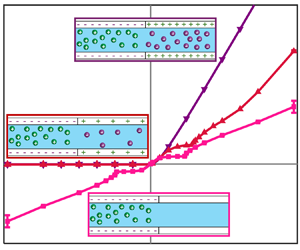
Schematic of the current density−voltage $(i\unicode{x2013} V)$ response curve for three different systems: unipolar systems, without and with EOF, and a bipolar system without EOF. The $i\unicode{x2013} V$ of the unipolar system comprises three distinct regions: the Ohmic (i.e. linear response regime), the limiting current density and the overlimiting current density responses. The bipolar response has a limiting current for negative voltages and currents of unconstrained values for positive voltages.

2.3 Current–voltage response of bipolar systems without EOF

Finally, we review the $i\unicode{x2013} V$ of bipolar systems without EOF. The $i\unicode{x2013} V$ of such systems is given by the dashed purple line in figure 2. There are countless outstanding experimental and numerical works investigating the $i\unicode{x2013} V$ of these systems – for brevity, we name but a few (Reference Siwy, Heins, Harrell, Kohli and MartinSiwy et al. 2004; Reference Vlassiouk, Smirnov and SiwyVlassiouk et al. 2008, Reference Vlassiouk, Kozel and Siwy2009; Reference He, Gillespie, Boda, Vlassiouk, Eisenberg and SiwyHe et al. 2009; Reference Picallo, Gravelle, Joly, Charlaix and BocquetPicallo et al. 2013; Reference Ható, Valiskó, Kristóf, Gillespie and BodaHató et al. 2017; Reference Mádai, Valiskó and BodaMádai, Valiskó & Boda 2019; Reference Lucas and SiwyLucas & Siwy 2020; Reference Córdoba, de Oca, Dhanasekaran, Darling and de PabloCórdoba et al. 2023) and refer the interested readers to the reviews (Reference Cheng and GuoCheng & Guo 2010; Reference Huang, Kong, Wen and JiangHuang et al. 2018; Reference Pärnamäe, Mareev, Nikonenko, Melnikov, Sheldeshov, Zabolotskii and TedescoPärnamäe et al. 2021) for a complete list. However, there are very few works that have considered the $i\unicode{x2013} V$ theoretically (reviewed below) – all of which assumed no EOF.

Reference Vlassiouk, Smirnov and SiwyVlassiouk et al. (2008) first derived a 1-D $i\unicode{x2013} V$ after assuming that the lengths of the positive and negative charged regions were equal, and that the charges of the positive region were minus that of the negative. Their model did not impose that the values of the excess counterion charges, to be defined later in § 3.2, were large or small. Later, Reference Picallo, Gravelle, Joly, Charlaix and BocquetPicallo et al. (2013) derived an alternative 1-D $i\unicode{x2013} V$ after assuming equal lengths. In contrast to Reference Vlassiouk, Smirnov and SiwyVlassiouk et al. (2008), they did not assume the charges were of equal magnitude (and opposite sign), but they did assume that the values of the excess counterion charges were large such that each charged region was ideally selective. Figure 3 compares the two non-dimensional $i\unicode{x2013} V$ responses with exact numerical simulations (the normalizations are outlined in § 3.2 below). It can be observed that the $i\unicode{x2013} V$ of Reference Vlassiouk, Smirnov and SiwyVlassiouk et al. (2008) holds for all values of V and ${N_2}$ (defined below), while the $i\unicode{x2013} V$ of Reference Picallo, Gravelle, Joly, Charlaix and BocquetPicallo et al. (2013) holds for all voltages, but only for very high values of ${N_2}$. However, it should be noted that the $i\unicode{x2013} V$ of Reference Picallo, Gravelle, Joly, Charlaix and BocquetPicallo et al. (2013) had another advantage – namely, their $i\unicode{x2013} V$ was also able to account for bulk asymmetric concentrations that were not accounted for in the other model.

Figure 3.

The (non-dimensional) current(-density)–voltage, $i\unicode{x2013} V$, curves comparing the two theoretical works of Reference Vlassiouk, Smirnov and SiwyVlassiouk, Smirnov & Siwy (2008) and Reference Picallo, Gravelle, Joly, Charlaix and BocquetPicallo et al. (2013), and 1-D numerical simulations for a bipolar system with varying values of excess counterion charge ${N_2}$: (a) ${N_2} = 2000$; (b) ${N_2} = 200$; (c) ${N_2} = 50$; and (d) ${N_2} = 10$. To allow for a straightforward analysis, here, we have assumed ${L_{2,3}} = 1$, ${N_2} ={-} {N_3}$ and that the effect of the diffusion layers is negligible such that ${L_{1,4}} = 0$.

We point out that the $i\unicode{x2013} V$ of Reference Vlassiouk, Smirnov and SiwyVlassiouk et al. (2008) was extended later by Reference Green, Edri and YossifonGreen, Edri & Yossifon (2015a), who derived a more general $i\unicode{x2013} V$ with three changes/modifications. First, their solution considered a 2-D geometry. Second, they discovered that one does not need to require symmetry in the geometry and anti-symmetry in the surface charges independently, but rather, there is a more general constraint – this constraint is discussed in § 4 more thoroughly. Third, they accounted for the diffusion layers. This is important because, in any realistic system (figure 1), the bipolar diode is connected to larger reservoirs that always need to be accounted for. Even without EOF, they contribute additional resistances. However, when EOF is accounted for, the instability that occurs forms at the interface of the bipolar diode with the diffusion layers.

3. Problem formulation

This work considers ion transport across a system comprising four layers: two diffusion layers and two oppositely charged permselective regions. Section 3.1 discusses the 2-D geometric set-up. Section 3.2 presents the governing equations. Section 3.3 supplements the boundary conditions (BCs). Section 3.4 briefly details the numerical methods and simulation parameters. Section 3.5 details various averaging operators repeatedly used in both Part 1 and Part 2.

3.1 Geometry

Figure 4 presents a 2-D system comprising four regions of uniform width W and various lengths ${L_k}$, where the index $k = 1,2,3,4$ denotes each region (top view of figure 1). The two outer regions (regions 1 and 4) are commonly termed ‘diffusion layers’ – these are uncharged regions filled with an electrolyte. Regions 2 and 3 are negatively and positively charged, respectively, permselective regions. In the following, we will use the ${\varDelta _k}$ notation to denote cumulative lengths within the system

(3.1a–d)\begin{equation}{\varDelta _1} = {L_1},\quad {\varDelta _2} = {\varDelta _1} + {L_2},\quad {\varDelta _3} = {\varDelta _2} + {L_3},\quad {\varDelta _4} = {\varDelta _3} + {L_4}.\end{equation}

Figure 4.

Schematic of a two-dimensional four-layered system comprising two diffusion layers (regions 1 and 4) connected by two permselective mediums (regions 2 and 3). The origin is in the bottom left corner of region 1. The width of the system is W, while the length of each region is given by ${L_k}$, $k = 1,2,3,4$. At the outer boundary of the diffusion layers, there are two bulk reservoirs with the same electrolyte maintained at an equal, fixed concentration and under a potential drop of V (defined as positive from $y = 0$ to $y = {\varDelta _4}$). The system is periodic at $x = 0$ and $x = W$ (denoted by dashed red lines). All boundary conditions are detailed in § 3.3. We account for EOF in the diffusion layers (regions 1 and 4), while in the permselective regions (regions 2 and 3), we do not (see § 3.2).

3.2 Governing equations

The non-dimensional time-dependent equations that govern ion transport through a permselective medium are the Poisson–Nernst–Planck and the Stokes equations. For a symmetric and binary electrolyte $({z_ + } ={-} {z_ - } = 1)$ with ions of equal diffusivities $({\tilde{D}_ \pm } = \tilde{D})$, the non-dimensional equations are

(3.2)\begin{gather}{\partial _t}{c_ \pm } = {-} \boldsymbol{\nabla }\boldsymbol{\cdot }{\boldsymbol{j}_ \pm } = \boldsymbol{\nabla }\boldsymbol{\cdot }(\boldsymbol{\nabla }{c_ \pm } \pm {c_ \pm }\boldsymbol{\nabla }\varphi ) - Pe\textrm{(}\boldsymbol{u}\boldsymbol{\cdot }\boldsymbol{\nabla }\textrm{)}{c_ \pm },\end{gather}

(3.3)\begin{gather}2{\varepsilon ^2}{\mathrm{\nabla }^2}\varphi = {-} {\rho _e},\end{gather}

(3.4)\begin{gather}\boldsymbol{\nabla }\boldsymbol{\cdot }\boldsymbol{u} = \textrm{0,}\end{gather}

(3.5)\begin{gather}-\boldsymbol{\nabla }p + {\mathrm{\nabla }^2}\boldsymbol{u}+ {\mathrm{\nabla }^2}\varphi \boldsymbol{\nabla }\varphi \textrm{ = 0}\textrm{.}\end{gather}

Note that, here and in Part 2, tilded notation is used for dimensional variables, whereas untilded variables are non-dimensional. Equation (3.2) is the Nernst–Planck equation satisfying continuity of ionic fluxes, ${\boldsymbol{j}_ \pm }$, for cation and anion concentrations, ${c_ + }$ and ${c_ - }$, respectively. The concentrations have been normalized by the bulk concentration ${\tilde{c}_0}$. The spatial variables have been normalized by a characteristic length $\tilde{L}$ ($\tilde{L}$ can be chosen arbitrarily as one of ${\tilde{L}_{1,2,3,4}}$ or $\tilde{W}$ so long as one of these lengths is set to unity). Time, $\tilde{t}$, has been normalized by the diffusion time ${\tilde{t}_D} = {\tilde{L}^2}/\tilde{D}$, and the ionic fluxes have been normalized by ${\tilde{j}_0} = \tilde{D}{\tilde{c}_0}/\tilde{L}$. Equation (3.3) is the Poisson equation for the electric potential, $\varphi$, which has been normalized by the thermal potential ${\tilde{\varphi }_{th}} = \tilde{\Re }\tilde{T}/\tilde{F}$, where $\tilde{\Re }$ is the universal gas constant, $\tilde{T}$ is the absolute temperature and $\tilde{F}$ is the Faraday constant. The parameter $\varepsilon $ is the non-dimensional Debye length,

(3.6a,b)\begin{equation}\varepsilon = \frac{{{{\tilde{\lambda }}_D}}}{{\tilde{L}}},\quad {\tilde{\lambda }_D} = \sqrt {\frac{{{{\tilde{\varepsilon }}_0}{\varepsilon _r}\tilde{\Re }\tilde{T}}}{{2{{\tilde{F}}^2}{{\tilde{c}}_0}}}} .\end{equation}

Herein, ${\tilde{\varepsilon }_0}$ and ${\varepsilon _r}$ are the permittivity of vacuum and the relative permittivity, respectively. The non-dimensional space charge density, ${\rho _e}$ (normalized by $\tilde{F}{\tilde{c}_0}$), in each of the regions, appearing on the right-hand side of (3.3), is given by

(3.7)\begin{equation}{\rho _e} = {c_ + } - {c_ - } - {N_2}{\delta _{2,k}} - {N_3}{\delta _{3,k}},\end{equation}

where ${\delta _{lk}}$ is Kronecker's delta and ${N_{2,3}}$ (${N_2} \ge 0$ and ${N_3} \le 0$) are the non-dimensional volumetric excess counterion charge densities in the permselective regions (normalized by $\tilde{F}{\tilde{c}_0}$) due to the surface charge densities, ${\tilde{\sigma }_s}$. In nanochannel systems, this relation is given by $N ={-} 2{\tilde{\sigma }_s}/\tilde{F}{\tilde{c}_0}\tilde{h}$, where $\tilde{h}$ is the height of the permselective region. Equations (3.4) and (3.5) are respectively the continuity equation for an incompressible solution and the Stokes equation obtained from the full momentum equation after omitting the nonlinear inertia terms due to a small Reynolds number. The non-dimensional velocity vector $\boldsymbol{u} = u\hat{\boldsymbol{x}} + v\hat{\boldsymbol{y}}$ and pressure p have been normalized respectively by a typical velocity ${\tilde{u}_0}$ and pressure ${\tilde{p}_0}$,

(3.8)\begin{equation}{\tilde{u}_0} = \frac{{{{\tilde{\varepsilon }}_0}{\varepsilon _r}\tilde{\varphi }_{th}^2}}{{\tilde{\mu }\tilde{L}}},\quad {\tilde{p}_0} = \frac{{\tilde{\mu }{{\tilde{u}}_0}}}{{\tilde{L}}},\end{equation}

where $\tilde{\mu }$ is the dynamic viscosity of the fluid. Note that the time derivative of the velocity has also been neglected since the Schmidt number ($Sc\textrm{ = }\tilde{\mu }/\textrm{(}\tilde{\rho }\tilde{D})$, where $\tilde{\rho }$ is the mass density) is large (Reference Rubinstein and ZaltzmanRubinstein & Zaltzman 2015). Correspondingly, the resulting non-dimensional Péclet number, $Pe$, in (3.2), defined as

(3.9)\begin{equation}Pe = \frac{{{{\tilde{u}}_0}\tilde{L}}}{{\tilde{D}}} = \frac{{{{\tilde{\varepsilon }}_0}{\varepsilon _r}\tilde{\varphi }_{th}^2}}{{\tilde{\mu }\tilde{D}}},\end{equation}

is an intrinsic material characteristic of the electrolyte, independent of the bulk concentration or characteristic length. As indicated by Reference Rubinstein and ZaltzmanRubinstein & Zaltzman (2000), for a typical aqueous low molecular electrolyte, $Pe$ is of the order of unity (discussed further below).

In this work, we have chosen a non-dimensional analysis that is drastically more robust than the dimensional analysis. For example, consider the expression for the excess counterion concentration $N ={-} 2{\tilde{\sigma }_s}/\tilde{F}{\tilde{c}_0}\tilde{h}$, which depends on three independent parameters, ${\tilde{\sigma }_s},{\tilde{c}_0}$ and $\tilde{h}$. Any combination of these parameters that yield the same N will have the same result. In these works, we will keep ${N_2}$ constant and large (such that ${N_2} \gg 1$) while we vary ${N_3}$. This is equivalent to changing the surface charge density in region 3. Note that the scenario ${N_3} = 0$ will reduce the system to an ideally selective unipolar system (whose response has been thoroughly investigated).

In this work, we focus on elucidating the effects of the EOI in a bipolar set-up. It is essential to realize that the effects of electroconvection manifest themselves differently in the diffusion layers versus the permselective regions. In practicality, the diffusion layers are regions comprising solely fluids and are dominated by bulk effects. In contrast, the permselective regions are either highly confined nanochannels or nanoporous membranes. In either situation, the effects of the surfaces, through the requirement of no slip and the effects of tortuosity, result in substantially smaller velocities (relative to what appears in the diffusion layers), such that the effect of the velocity is virtually zero. To that end, and to reduce computational costs, we a priori assume the velocity field in the permselective regions is zero (Reference Rubinstein and ZaltzmanRubinstein & Zaltzman 2015; Reference Abu-Rjal, Rubinstein and ZaltzmanAbu-Rjal, Rubinstein & Zaltzman 2016; Reference Abu-Rjal, Prigozhin, Rubinstein and ZaltzmanAbu-Rjal et al. 2017; Reference Ganchenko, Kalaydin, Ganchenko and DemekhinGanchenko et al. 2018). In other words, in regions 1 and 4, we solve (3.2)–(3.5), while in regions 2 and 3, we solve only (3.2) and (3.3).

3.3 Boundary conditions

The boundary conditions for the closure of the governing equations (3.2)−(3.5) are given below. At the stirred bulk reservoirs, we have a bulk solution with the same electrolyte maintained at an equal, fixed concentration that is experiencing no shear stress and zero inflow into the system and under a potential drop of $V$ (crimson and blue lines located at $y = 0$ and $y = {\varDelta _4}$, respectively, in figure 4),

(3.10)\begin{gather}y = 0:{c_ \pm } = 1,\quad {\partial _y}u = 0,\quad v = 0,\quad \varphi = V,\end{gather}

(3.11)\begin{gather}y = {\varDelta _4}:{c_ \pm } = 1,\quad {\partial _y}u = 0,\quad v = 0,\quad \varphi = 0.\end{gather}

At all the internal interfaces, located at $y = {\varDelta _1},{\varDelta _2},{\varDelta _3}$ (pink lines in figure 4), we require continuity of the normal ionic fluxes and electric field

(3.12a,b)\begin{equation}y = {\varDelta _1},{\varDelta _2},{\varDelta _3}:[\,{\boldsymbol{j}_ \pm }\boldsymbol{\cdot }\boldsymbol{n}] = 0,\quad [ - \boldsymbol{\nabla }\varphi \boldsymbol{\cdot }\boldsymbol{n}] = 0,\end{equation}

where $[ \ldots ]$ represents the differences across the interfaces and n is the unit normal vector. At the interfaces between the diffusion layers and permselective regions, we impose the common no-slip condition

(3.13)\begin{equation}y = {\varDelta _1},{\varDelta _3}:\boldsymbol{u}\textrm{ = }{\bf 0}{\bf .}\end{equation}

We complete the boundary conditions by prescribing periodicity at $x = 0$ and $x = W$ (dashed red lines in figure 4),

(3.14a,b)\begin{equation}f(0,y,t) = f(W,y,t),\quad {\partial _x}f(0,y,t) = {\partial _x}f(W,y,t),\end{equation}

where f corresponds to all the variables in (3.2)–(3.5) (i.e. ${c_ \pm }$, $\varphi$, $\boldsymbol{u}$ and $p$).

3.5 Averaging operators

To characterize the system response, we use both time and spatial averages of any quantity f (e.g. ${c_ \pm }$, $\varphi $, ${\rho _e}$, and their fluxes, etc.). Here, we define the operators and their notation. The spatial average across the x-direction is denoted with an overbar and defined as

(3.15)\begin{equation}\bar{f}(y,t) = \frac{1}{W}\int_0^W {f(x,y,t)\,\textrm{d}x} .\end{equation}

The surface average over any region k is denoted with two overbars and defined as

(3.16)\begin{equation}{\bar{\bar{f}}_{k = 1,4}}(t) = \frac{1}{{{L_{k = 1,4}}}}\int_{{L_{k = 1,4}}} {\bar{f}(y,t)\,\textrm{d}y} .\end{equation}

To calculate steady-state results of either (3.15) or (3.16), we define the temporal average,

(3.17a,b)\begin{equation}\langle \bar{f}\rangle = \frac{1}{T}\int_{{t_0}}^{{t_0} + T} {\bar{f}\,\textrm{d}t} ,\quad \langle \bar{\bar{f}}\rangle = \frac{1}{T}\int_{{t_0}}^{{t_0} + T} {\bar{\bar{f}}\,\textrm{d}t} ,\end{equation}

where ${t_0}$ is the time at which the system reaches a state where the state is perturbed about a ‘steady-state’ (i.e. a statistically steady-state), and T is the time duration of this ‘steady-state’ (typically the end of the simulations). This average is denoted with angle brackets (chevron brackets).

Of particular importance is the average of the electrical current density, $\tilde{\boldsymbol{i}} = {\tilde{i}_x}\hat{\boldsymbol{x}} + {\tilde{i}_y}\hat{\boldsymbol{y}}$. The non-dimensional electrical current density (normalized by $\tilde{F}\tilde{D}{\tilde{c}_0}/\tilde{L}$) is defined as

(3.18)\begin{equation}\boldsymbol{i} = {\boldsymbol{j}_ + } - {\boldsymbol{j}_ - } = Pe({c_ + } - {c_ - })\boldsymbol{u} - \boldsymbol{\nabla }({c_ + }{\bf - }{c_ - }) - ({c_ + } + {c_ - })\boldsymbol{\nabla }\varphi .\end{equation}

In the remainder, we will consider the time-dependent x-average of the normal component of the electrical current density, ${i_y}(t)$, at $y = 0$ given by

(3.19)\begin{equation}\bar{i}(t) = \frac{1}{W}\int_0^W {{i_y}(x,y = 0,t)\,\textrm{d}{\kern0.8pt}x} .\end{equation}

Another important characterizer of the flow, which will be used throughout this work, is the kinetic energy density (energy per unit volume), ${\tilde{E}_k}$, in the diffusion layers. The non-dimensional kinetic energy density (normalized by $\tilde{\rho }\tilde{u}_0^2$) is defined as

(3.20)\begin{equation}{E_k} = {\textstyle{1 \over 2}}|\boldsymbol{u}{|^2} = {\textstyle{1 \over 2}}({u^2} + {v^2}),\end{equation}

and ${E_k}$ will, often, be subject to any one of the operators given by (3.15)–(3.17).

Finally, we note that, in general, the $\langle \bar{i}\rangle \unicode{x2013} V$ response is asymmetric around $V = 0$. The degree of asymmetry is characterized by the rectification factor, $RF$ (Reference Vlassiouk, Smirnov and SiwyVlassiouk et al. 2008, Reference Vlassiouk, Kozel and Siwy2009; Reference Cheng and GuoCheng & Guo 2010),

(3.21)\begin{equation}\left\langle {\overline {RF} } \right\rangle = \left|{\frac{{{{\langle \bar{i}\rangle }_{V > 0}}}}{{{{\langle \bar{i}\rangle }_{V < 0}}}}} \right|.\end{equation}

In the remainder, we will also make a comparison of the rectification factor. Specifically, we will consider the current mean as well as the current fluctuations. Note that even though $\langle {\overline {RF} } \rangle$ is defined by (3.21), there is some ambiguity as to how the mean is calculated. In general, one should calculate the mean of the ratio and not the ratio of the means. However, this raises both conceptual difficulties as well as numerical difficulties. To that end, we have found that the ratio of the means is the simplest metric to compare two different states of positive and negative voltages. This definition is loosely related to the concept of error propagation (Reference Sipkens, Corbin, Grauer and SmallwoodSipkens et al. 2023)

(3.22)\begin{equation}{\sigma _{\overline {RF} }} = \left\langle {\overline {RF} } \right\rangle \sqrt {{{\left( {\frac{{{\sigma_{\bar{i},V > 0}}}}{{{{\langle \bar{i}\rangle }_{V > 0}}}}} \right)}^2} + {{\left( {\frac{{{\sigma_{\bar{i},V < 0}}}}{{{{\langle \bar{i}\rangle }_{V < 0}}}}} \right)}^2}} .\end{equation}

Here, we have ${\sigma _{\overline {RF} }}$, using the mean current, $\langle \bar{i}\rangle$, and the current density standard deviation, ${\sigma _{\bar{i}}}$, for positive and negative voltages. It can be noted that the ‘total’ standard deviation depends on $\langle {\overline {RF} } \rangle$, and the mean and standard deviation of each scenario (positive and negative voltages) in an independent manner.

4. Steady-state results

In the following, we will present the non-dimensional steady-state response (time- and space-averaged based on (3.17)) $\langle \bar{i}\rangle \unicode{x2013} V$ for three scenarios (unipolar, non-ideal bipolar and ideal bipolar) without and with EOF.

The unipolar system is a three-layered system that includes only one permselective region. As a result, if both flanking microchannels have the same geometry, the $\langle \bar{i}\rangle \unicode{x2013} V$ is symmetric around $V = 0$. If the flanking microchannels are asymmetric, so too is the $\langle \bar{i}\rangle \unicode{x2013} V$. These statements hold regardless of whether EOF is included or not. This will be demonstrated shortly.

Bipolar systems, comprising four layers and including two charged regions of opposite charges, have an inherently more complicated response. In fact, the fourth layer adds an additional degree of freedom, which leads to a parameter that marks the difference between non-ideal and ideal bipolar systems. The parameter that determines the response is a parameter that accounts for the geometric and excess counterion charge density of both permselective regions (see Reference Green, Edri and YossifonGreen et al. (2015a) for the 2-D version of this equation)

(4.1)\begin{equation}\eta = \frac{{{L_3}}}{{{L_2}}} \times \left|{\frac{{{N_3}}}{{{N_2}}}} \right| = \left\{ {\begin{array}{@{}ll@{}} 0&{\textrm{unipolar}}\\ {0 < \eta < 1}&{\textrm{non-ideal}\;\textrm{bipolar.}}\\ 1&{\textrm{ideal}\;\textrm{bipolar}} \end{array}}\right.\end{equation}

It is trivial to see that when either ${N_3} = 0$ or ${L_3} = 0$, the second charged region does not exist, and the bipolar system reduces to the unipolar system. If, however, there are two charged regions, the ratio $\eta$ will determine the overall response of the system. If $\eta = 1$ (and ${L_2} = {L_3}$), the total excess counterion charges in both regions are equal (but of opposite sign), and the response is what we now term ‘ideal’ bipolar. If $1 > \eta > 0$, we term the response non-ideally bipolar. The non-ideal bipolar system will exhibit time-dependent and steady-state characteristics of both unipolar and ideal bipolar systems.

Before continuing with our analysis, we wish to make a distinction in the terminology adopted in this work relative to our previous work (Reference Abu-Rjal and GreenAbu-Rjal & Green 2021). In that work, the $\eta = 1$ scenario was termed a ‘symmetric’ bipolar system, while the $1 > \eta > 0$ scenario was termed an ‘asymmetric’ bipolar system. At that time, our choice of using the words ‘symmetry’ and ‘asymmetry’ was to emphasize whether there was a symmetry between the total excess counterion charges in both regions. However, $\eta$ does not determine whether the response will be symmetric or not since, in a bipolar system, the response is always asymmetric. Thus, in this work, we see fit to update and change our past terminology such that we now state that $\eta$ determines whether the $\langle \bar{i}\rangle \unicode{x2013} V$ response is that of an ‘ideal’ bipolar response or a non-ideal bipolar response.

In our numerical simulations, we keep the geometry constant such that ${L_{1,2,3,4}} = 1$. We set ${N_2} = 25$, while varying ${N_3}$. In doing so, we vary the ratio $|{N_3}|/|{N_2}|$. For the sake of simplicity, our initial discussion will focus only on the three scenarios of ${N_3} ={-} 25$, ${N_3} ={-} 10$ and ${N_3} = 0$ corresponding to our three scenarios of ideal bipolar, non-ideal bipolar and unipolar, respectively. After we have delineated the differences between the three scenarios, we will present a more systematic analysis of the full range of ${N_3}$ values considered.

Before presenting the comparison of the three scenarios, one last comment is needed. By setting ${N_3} = 0$, a four-layered system effectively becomes a three-layered system. To allow for a straightforward comparison of all aforementioned scenarios, we have chosen to keep the overall length of the system the same. Thus, in the unipolar scenario shown in the comparison, we have made the effective length of one of the diffusion layers to ${L_3} + {L_4} = 2$. This contrasts with the more standard case of symmetric diffusion layer lengths, where ${L_3} + {L_4} = 1$. For the sake of completion, we now demonstrate that the qualitative response of these two unipolar systems remains unchanged, with the sole difference being that the system with an asymmetric geometry has a non-unity rectification factor (Reference Green, Edri and YossifonGreen et al. 2015a).

Figure 5(a) compares the non-dimensional steady-state $\langle \bar{i}\rangle \unicode{x2013} V$ response between two unipolar systems: symmetric (${L_4} = {L_1}$, blue lines and circle markers) and asymmetric (${L_4} = 2{L_1}$, pink lines and square markers). Both responses with EOF exhibit all three current regions described in § 2.2 (and shown schematically in figure 2). The symmetric system has a (anti-)symmetric response around $V = 0$. In contrast, the asymmetric system has an asymmetric response. The degree of asymmetry is quantified through the rectification factor, $\langle {\overline {RF} } \rangle$, plotted in figure 5(b). Naturally, for the symmetric case, $\langle {\overline {RF} } \rangle \equiv 1$, while for the asymmetric case, our chosen asymmetry leads to $\langle {\overline {RF} } \rangle > 1$. While we find that $\langle {\overline {RF} } \rangle$ is enhanced by EOF, our numerical simulations show that above $V \simeq 50$, the rectification factor plateaus. This ratio is likely set by geometry – and should be investigated in future works.

Figure 5.

(a) The (non-dimensional) steady-state current-density–voltage, $\langle \bar{i}\rangle \unicode{x2013} V$, curves, without and with EOF, for symmetric (${L_1} = {L_4}$, blue lines) and asymmetric ($2{L_1} = {L_4}$, red lines) unipolar systems (time- and space-averaged based on (3.17)). Note that systems with EOF have the three distinct regions described previously (figure 2). Insets show the time and surface average of the kinetic energy, $\langle {\overline {\overline {{E_k}} } }\rangle$, for negative and positive voltages. (b) Rectification factor versus the voltage. The error bars in panel (a) denote one standard deviation of the current, while the error bars in panel (b) denote the standard deviation defined by (3.22).

Figure 6 shows the $\langle \bar{i}\rangle \unicode{x2013} V$ for the three scenarios without EOF (dashed lines) and with EOF (solid lines with markers). For the sake of comparison, here we show the asymmetric unipolar response previously discussed in figure 5 and compare it to the two other bipolar scenarios. Notice that the ideal bipolar exhibits a rather remarkable result. The $\langle \bar{i}\rangle \unicode{x2013} V$ with EOF completely coincides with the $\langle \bar{i}\rangle \unicode{x2013} V$ without EOF. This remarkable result is due to $\eta = 1$, where the internal ‘symmetry’ of positive and negative charges leads to a ‘symmetry’ in the fluxes. We will further discuss this in the next paragraph. The non-ideal bipolar system exhibits equally remarkable but substantially different behaviour. For negative voltages, the $\langle \bar{i}\rangle \unicode{x2013} V$ with EOF coincides with the $\langle \bar{i}\rangle \unicode{x2013} V$ without EOF, as in the case of the ideal bipolar system. In contrast, for positive voltages, the $\langle \bar{i}\rangle \unicode{x2013} V$ with EOF breaks from the $\langle \bar{i}\rangle \unicode{x2013} V$ without EOF, as in the case of a unipolar system. This, too, will be discussed shortly. Also, we note that for negative voltages, both bipolar systems exhibit limiting currents (even with EOF) that are not observed for the unipolar system with EOF.

Figure 6.

The (non-dimensional) steady-state current density-voltage, $\langle \bar{i}\rangle \unicode{x2013} V$, results without EOF (dashed lines) and with EOF (solid lines and markers) for three scenarios: unipolar $({N_3} = 0)$, non-ideal bipolar $({N_3} ={-} 10)$ and ideal bipolar $({N_3} ={-} 25)$ systems. The inset is a zoomed view of the negative voltage near $\langle \bar{i}\rangle = 0$, showing that the $\langle \bar{i}\rangle \unicode{x2013} V$ curves of bipolar systems do not exhibit OLCs there. The error bars denote one standard deviation of the current.

To understand why the ideal bipolar scenario with EOF does not exhibit a difference relative to the scenario without EOF, we must return to the problem definition in § 3.2 (see last paragraph), where we assumed that the velocity within the permselective material is zero. Essentially, independent of what is occurring within the diffusion layers, we have constrained the response of the bipolar membrane (regions 2 and 3) to be identical to the response of a bipolar membrane in the convectionless scenario. This is immensely important since the $\langle \bar{i}\rangle \unicode{x2013} V$ for the $\eta = 1$ scenario (discussed in § 2.3 and shown in figure 2) assumes that the steady-state salt current density, $j = {j_ + } + {j_ - }$, is zero $(j = 0)$ such that ${j_ + } ={-} {j_ - }$ (Reference Green, Edri and YossifonGreen et al. 2015a). From the steady-state point of view, we realize that by virtue of the internal symmetry, for every positive ion transported from region 1 to region 4, there is a negative ion transported from region 4 to region 1. These counter fluxes are responsible for stabilizing the extended space charge layer that forms in each of the regions. The convection-less dynamics have been discussed thoroughly in our past work (Reference Abu-Rjal and GreenAbu-Rjal & Green 2021), and the dynamics with convection will be discussed in Part 2. However, if one removes the $\eta = 1$ condition, then $j \ne 0$. Thus, non-ideal bipolar systems do exhibit overlimiting currents.

Our last comment pertaining to figure 6 is with regards to negative voltages. For a unipolar system, overlimiting currents are observed, while for bipolar systems, they are not. This is because for unipolar systems, there is no inherent difference between the two diffusion layers and the switch of $V > 0$ with $V < 0$ (or vice versa, see figure S4 in the supplementary material). This is in contrast to bipolar systems, where the internal (and inherent) electric field from the positive region (here, region 2) to the negative region (here, region 3) leads to a change in the behaviour of the dynamics of the diffusion layers when $V > 0$ and $V < 0$ are switched. Here, too, the convection-less dynamics has been discussed thoroughly in our past work (Reference Abu-Rjal and GreenAbu-Rjal & Green 2021), and the dynamics with convection will be discussed in Part 2.

Finally, figure 7 presents a thorough scan for varying values of ${N_3}$ (and thus, $\eta $). Figure 7(a) shows the steady-state $\langle \bar{i}\rangle \unicode{x2013} V$ for several values of ${N_3}$ without EOF (dashed lines) and with EOF (solid lines). We vary ${N_3}$ from a unipolar scenario (${N_3} = 0$ given by the pink line) and an ideal bipolar scenario (${N_3} ={-} {N_2} ={-} 25$ given by the purple line). Save for some quantitative differences, all the non-ideal diodes behave similarly to the one discussed in figure 6. The changes in all the steady-state $\langle \bar{i}\rangle \unicode{x2013} V$ responses can be correlated to the steady-state kinetic energy (figure 7c) – the larger the kinetic energy, the stronger the mixing is, and with it comes an increased current (figure S5 in the supplementary material shows that as the voltage drop is increased, the vortex array loses its stable structure, and a more chaotic and efficient mixing takes place – a similar result was shown by Reference Druzgalski, Andersen and ManiDruzgalski, Andersen & Mani 2013). Supplementary material figure S6 shows that the critical voltage, ${V_{cr}}$, varies as ${N_3}$ is varied. Two interesting limits are noteworthy. For the ideal bipolar response, the critical voltage is substantially increased. For the unipolar scenario, the critical voltage is the smallest (~20). This value is similar to the linear stability analysis prediction by Reference Zaltzman and RubinsteinZaltzman & Rubinstein (2007), Reference Demekhin, Nikitin and ShelistovDemekhin, Nikitin & Shelistov (2013), Reference Abu-Rjal, Rubinstein and ZaltzmanAbu-Rjal et al. (2016) and those found in the numerical simulations of Reference Demekhin, Nikitin and ShelistovDemekhin et al. (2013), Reference Druzgalski, Andersen and ManiDruzgalski et al. (2013). Future works should follow the works of Reference Zaltzman and RubinsteinZaltzman & Rubinstein (2007), Reference Demekhin, Nikitin and ShelistovDemekhin et al. (2013, Reference Demekhin, Nikitin and Shelistov2014), and undertake a linear stability analysis to investigate the critical voltage. One last comment regarding figure 7(c) is needed. Figure S7 shows that we can fit the kinetic energy to be a parabolic profile such that $\langle {\overline {\overline {{E_k}} } } \rangle = \alpha ({N_3}){[V - {V_{cr}}]^2} + \beta ({N_3})$. Here, $\alpha ({N_3})$ and $\beta ({N_3})$ are fitting parameters that depend on ${N_3}$ (and possibly ${N_2}$). We are currently unable to rationalize this result – and perhaps this, too, will be resolved within the future work that conducts the linear stability analysis.

Figure 7.

The (non-dimensional) steady-state voltage-dependent results for (a) the current density–voltage response, $\langle \bar{i}\rangle \unicode{x2013} V$, (b) a semilog₁₀ plot of the rectification factor, (c) the surface average of the kinetic energy, $\langle {\overline {\overline {{E_k}} } } \rangle$, in region 1, and (d) the cationic transport number, $\langle {\bar{\tau }_ + }\rangle $, for the scenarios without EOF (dashed lines) and with EOF (solid lines and markers) for several values of ${N_3}$. The inset of panel (a) is the $\langle \bar{i}\rangle \unicode{x2013} V$ for negative voltages. The vertical bars denote one standard deviation error bar.

Unsurprisingly, as the kinetic energy increases, so does the rectification factor (figure 7b). However, the increases in the currents and the rectification factor are not without consequences. From figure 7(d), we can observe that the transport number

(4.2)\begin{equation}{\tau _ + } = \frac{{{j_ + }}}{{{j_ + } - {j_ - }}} = \frac{1}{2}\left( {1 + \frac{j}{i}} \right),\end{equation}

which is a proxy for the overall selectivity of the channel (Reference Abu-Rjal, Chinaryan, Bazant, Rubinstein and ZaltzmanAbu-Rjal et al. 2014; Reference Green, Abu-Rjal and EshelGreen, Abu-Rjal & Eshel 2020), decreases with decreasing ${N_3}$ and with the inclusion of EOF. In a unipolar system, when ${\tau _ + } \equiv 1$, the system is ideally selective, while ${\tau _ + } \equiv 1/2$ corresponds to a vanishingly selective system. However, such a definition is not simple for bipolar systems, where one of the components is ideally selective, and the other is not (see § 4.2 of Reference Abu-Rjal and GreenAbu-Rjal & Green (2021) for a thorough discussion on the permselective capability of each region separately versus that of the entire system). The reduction in the transport number, which could be detrimental to desalination, should be considered in future works.

Before proceeding to the discussion, we return to our previous statement (given in § 1) that most nanoporous materials and nanochannels behave the same. This statement is true in so far as all the major transport characteristics remain unchanged. Namely, the Ohmic conductance and the limiting currents predicted for all systems are rather independent of whether the system is 1-D, 2-D or 3-D. In contrast, we expect that the overlimiting current response of the system will vary as the geometry and the many boundary conditions are varied. This statement should be somewhat intuitive. First, it has been shown that the electroconvective instability is incapable of forming in a purely 1-D system (Reference Rubinstein and ZaltzmanRubinstein & Zaltzman 2000). However, if one then considers a 2-D system, where the width of the diffusion layers and the permselective materials are the same, the instability does appear above critical voltages. Such a 2-D system is quasi-1-D at low voltages, but 2-D at over-critical voltages. A similar statement holds for 3-D systems. All systems in which the diffusion layers and the permselective materials have the same height and width are termed ‘homogeneous’ systems. Except for the fact that 2-D and 3-D homogeneous systems can predict the instability, they can also be made to further differ from pure 1-D systems in the following manner. In our work, as in most works, one typically assumes that the system is periodic (equation (3.14)). Such an assumption is tantamount to assuming that the width and length of the system are infinite and that the effects of the outer boundaries are negligible. However, this does not need to be the case. For example, if at $x = 0,W$, there are walls, the periodic BC should be replaced with no-flux $({\boldsymbol{j}_ \pm }\boldsymbol{\cdot }\boldsymbol{n} = 0,\; - \boldsymbol{\nabla }\varphi \boldsymbol{\cdot }\boldsymbol{n} = 0)$ and no-slip $(\boldsymbol{u} = 0)$ BCs. The past work of Reference Abu-Rjal, Leibowitz, Park, Zaltzman, Rubinstein and YossifonAbu-Rjal et al. (2019) on unipolar systems has shown that the ‘overall’ response of the system does not change in the following manner: overlimiting currents still appear. However, both the time-transient and steady values of this scenario varied slightly relative to the purely homogeneous state. In changing the BC from an infinite system to a finite-size system, the effects of ‘confinement’ have been introduced. In general, we believe that so long as the height and width of homogeneous systems are large enough, then the robustness of the EOI will be the primary determinant of the system, and the response will not vary substantially.

There is yet another way to introduce the effects of confinement into the system. Consider systems in which the permselective material interface is smaller than the interface of the diffusion layers (i.e. a simple nanochannel system). These are called ‘heterogeneous’ systems. The introduction of heterogeneity also requires the change of boundary conditions at the permselective interface (some regions will use those given in (3.12), while others will require no flux). While the effects of heterogeneity in overlimiting conditions are not fully understood, they are understood in underlimiting conditions. Several works have shown that the Ohmic conductance and limiting currents can be theoretically predicted (Reference RubinsteinRubinstein 1991; Reference Rubinstein, Zaltzman and PundikRubinstein, Zaltzman & Pundik 2002; Reference Green, Shloush and YossifonGreen, Shloush & Yossifon 2014; Reference Green and YossifonGreen & Yossifon 2014). These underlimiting predictions were later confirmed experimentally (Reference Green, Park and YossifonGreen, Park & Yossifon 2015b; Reference Green, Eshel, Park and YossifonGreen et al. 2016). While these models have been very useful for predicting the underlimiting response and some of the trends observed for overlimiting responses, they are not capable of explaining the measurements of a confined heterogeneous system in which the critical voltage for overlimiting current increases as the degree of confinement is increased (Reference Yossifon, Mushenheim and ChangYossifon, Mushenheim & Chang 2010). Several numerical models focused on this problem (Reference Schiffbauer, Demekhin and GanchenkoSchiffbauer, Demekhin & Ganchenko 2012; Reference Andersen, Wang, Schiffbauer and ManiAndersen et al. 2017), in which a Hele-Shaw term was added to account for this confinement. However, these models typically assume that the system is a confined homogeneous system.

This work has considered the scenario of a 2-D unconfined periodic system in a bipolar system. Future works should focus on increasing the level of complexity by considering either non-periodic BCs or heterogeneous systems, or both. We reiterate that depending on the scenario, we expect that the overall robustness of the response of the system will remain unchanged. However, we also expect that there will be conditions in which the response changes drastically.