


Introduction
Previous research found that genetic profiles help predict key cattle growth traits in bull (Vestal et al., Reference Vestal, Lusk, DeVuyst and Kropp2013), feeder (DeVuyst et al., Reference DeVuyst, Biermacher, Lusk, Mateescu, Blanton, Swigert, Cook and Reuter2011), and live cattle selection (Holt, Reference Holt2010; Thompson et al., Reference Thompson, DeVuyst, Brorsen and Lusk2014), but there has been little research on the relationship between genotypic panel scores and economically relevant cow-calf production variables. Further, traits that are desirable in feedlot cattle production are potentially deleterious for cow-calf operations. For example, increased cow weights may not correlate with increased cow-calf profitability (Bir et al., Reference Bir, DeVuyst, Rolf and Lalman2018; Feuz, Russell, and Feuz, Reference Feuz, Russell and Feuz2021). The goal here is to determine the net value of these genetic traits in the cow-calf sector by estimating their effect on calf birth weight, weaning weight, and cow weight and then using these estimates to determine the effect on expected profit.
Genetic testing in beef cattle started with testing for the leptin gene in the 1990s, and the tests focused on single nucleotide polymorphisms (SNPs) that were associated with fat deposition (Fitzsimmons et al., Reference Fitzsimmons, Schmutz, Bergen and McKinnon1998). The leptin gene predicted intramuscular and external carcass fat and showed promise to increase feedlot profitability for cattle priced on a grid. While the leptin gene had little to no effect on days on feed and thus there was little value to sorting cattle, it was important in feeder cattle selection with differences up to $48 per head between the different SNPs (DeVuyst et al., Reference DeVuyst, Bullinger, Bauer, Berg and Larson2007). Although genetic testing in cattle showed promise for increasing profitability (Mitchell et al., Reference Mitchell, DeVuyst, Bauer and Larson2009), testing for the leptin gene in feedlot cattle was abandoned after a few years (Van Eenennaam and Drake, Reference Van Eennaam and Drake2012). In recent years, tests for the leptin gene have been replaced by genomic marker panels. These tests use dozens of SNPs for predicting desired outcomes (Thompson, Reference Thompson2018).
Thompson et al. (Reference Thompson, DeVuyst, Brorsen and Lusk2014) found that using genetic marker panels for management decisions and sorting cattle resulted in values of around $1 per head for each trait evaluated. Using panel scores to market cattle, however, resulted in a range of values from $1 to $13 per head depending on the structure of the grid (Thompson et al., Reference Thompson, DeVuyst, Brorsen and Lusk2016). The value of these tests, however, was not enough to offset the cost of testing (the Igenity Feeder profile was $15 in 2022). In 2016, the Igenity Gold profile studied here cost $40, but the cost of the comparable Igenity Beef Profile has since fallen to $29 per test and now includes 17 panel scores instead of 13 (Neogen, 2022). Selecting cattle based on genomic marker panels is expected to yield more than using the panels for management decisions alone (Thompson et al., Reference Thompson, DeVuyst, Brorsen and Lusk2014). The expected value of selecting for a single trait was $22, and the value associated with selecting for multiple traits was $38 (Thompson et al., Reference Thompson, DeVuyst, Brorsen and Lusk2014). The differences in value between these genetic differences are high, especially in bull testing (Vestal et al., Reference Vestal, Lusk, DeVuyst and Kropp2013). The incomplete adoption of marker panels in bull selection could be due to a market inefficiency due to asymmetric information (Maples et al., Reference Maples, DeVuyst and Brorsen2022), which causes cow-calf producers with better feedlot genetics to not be fully rewarded. Testing for genomic panel scores is now used mostly for breeding animals and even for breeding animals the use of panel scores is not common.
Results from hedonic pricing models show that cow-calf producers did not initially consider available genetic information when selecting or replacing herd bulls (Irsik et al., Reference Irsik, House, Shuffitt and Shearer2008). Rather than focusing on genetics, the price of a bull was highly dependent on breed, with preference toward Angus, age, and lower birth weights. Expected progeny differences (EPDs) are increasingly used in cattle selection, with Boyer et al. (Reference Boyer, Campbell, Griffith, DeLong, Rhinehart and Kirkpatrick2019), Vestal et al. (Reference Vestal, Lusk, DeVuyst and Kropp2013), and Tang et al. (Reference Tang, Thompson, Boyer, Widmar, Lusk, Stewart, Lofgren and Minton2023) concluding that EPDs were statistically significant determinants of bull prices.
Cow-calf producers have shifted their production practices over the last few decades resulting in higher mature cow weights (Bir et al., Reference Bir, DeVuyst, Rolf and Lalman2018; Feuz, Russell, and Feuz, Reference Feuz, Russell and Feuz2021). This shift in weights was due to a push to produce for feedlot profitability rather than cow-calf profitability (Bir et al., Reference Bir, DeVuyst, Rolf and Lalman2018). A concern is that traits that are positive for feedlots could be negative for cow-calf producers. Previous studies did not examine the effects of Igenity panel scores at the cow-calf producer level and only offer insight into the value of selecting for these traits at the feedlot level (DeVuyst et al., Reference DeVuyst, Biermacher, Lusk, Mateescu, Blanton, Swigert, Cook and Reuter2011; Thompson et al., Reference Thompson, DeVuyst, Brorsen and Lusk2014, Reference Thompson, DeVuyst, Brorsen and Lusk2016). This research aims to overcome these gaps and combine the impacts of genetic panel scores from a cow-calf operation with previously estimated impacts on feedlot operations to evaluate the potential for misaligned economic incentives in the beef industry.
Herds have shifted to a more feedlot-driven genetic composition with an emphasis on muscle, growth, and carcass quality in the last few decades (Bir et al., Reference Bir, DeVuyst, Rolf and Lalman2018; Smith, Reference Smith2014). What traits, if any, are correlated with higher weaning weights, optimal cow weights, or increased producer profitability? Does the optimal selection of Igenity panel scores for the entire beef sector differ from those that benefit cow-calf operators? Genetic traits as measured by Igenity panel scores are readily available and producers as well as the whole cattle industry can benefit from knowing more about how best to use this information.
Data collection
Hair follicle samples were taken from cows, steers, heifers, and bulls at weaning or purchase across four ranches in southern Oklahoma owned and operated by the Noble Research Institute (NRI). The NRI herds are managed by PhD animal scientists and are managed to demonstrate the optimal level of management. These samples were sent to Neogen to determine the Igenity genetic profile for each animal. Here, 13 Igenity panel scores are used including birth weight, calving ease direct, calving ease maternal, stayability, heifer pregnancy, docility, milk, residual feed intake, average daily gain, tenderness, marbling, ribeye area, and fat thickness. The Neogen profiles are on a scale of 1–10. The panel scores predict equal increments of the targeted trait. For example, each unit higher panel score for birth weight predicts a birth weight that is 1.3 lb. higher.
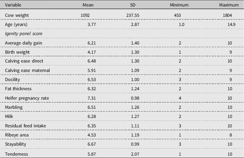
Data were collected for 1,205 calves born and weaned on the NRI ranches during 2015 through 2020. Table 1 shows summary statistics for all calf events and panel scores. Data were collected for 1,544 cows, providing 10,156 cow weights. Cow data include mature cows, first-calf heifers, bred heifers, exposed heifers, and replacement heifers all over one year old. These weights were captured at the chute during pregnancy checks, breeding, veterinary applications, and weight checks from 2015 to 2020. There are more observations on cows since collection of data on cows began before collection of data on calves. Table 2 reports the summary statistics of cow weights. Note that calf panel scores were used for the calves as compared to using dam panel scores because the calf panel scores were always available, while many of the dam scores were not. Using dam panel scores to measure the genetic effect on calves could have different results from this study, especially for the maternal traits. In particular, the dam’s milk score would likely have provided more information about weaning weight than the calf’s milk score.
Calf summary statistics (n = 1,205)

Cow weight summary statistics (n=10,156)
Note: Cows were weighed multiple times in each year. Replacement heifers included.
The four cow/calf herds were located on four different ranches. The ranches are Oswalt Road Ranch (OR) located near the community of Oswalt, OK (33°59'24.5"N 97°15'16.1"W), D. Joyce Coffey Ranch (CR) located near the community of Marietta, OK (33°56'03.5"N 97°13'38.6"W), Pasture Research and Demonstration Farm (PRDF) located near the community of Ardmore, OK (34°13'06.6"N 97°12'14.4"W), and the Red River Research and Demonstration Farm (RRF) located near the community of Burneyville, OK (33°52'56.5"N 97°16'03.5"W). CR and OR are predominantly comprised of native prairie grass and PRDF and RRF have introduced bermudagrass pasture. Hay and protein cubes were fed in the winter months. Angus (bos taurus) cows were artificially inseminated following the 7-day CoSynch (Bridges et al., Reference Bridges, Lake, Lemenager and Claeys2008) synchronization program. At CR and OR ranches, cattle were artificially inseminated with Angus semen with Charolais bulls turned out within 24 hours upon insemination. At PRDF, Angus cows sired by Hereford bulls followed a natural 60-d breeding program.
Igenity panel scores predict future progeny performance in comparison to the progeny of other animals (Neogen, 2021). The panels include two to over 100 SNPs (DeVuyst et al., Reference DeVuyst, Biermacher, Lusk, Mateescu, Blanton, Swigert, Cook and Reuter2011), but the exact number is proprietary. Higher Igenity panel scores are not always better but indicate the animal has a higher genetic potential for that trait. Table 3 provides a description of each trait and its desired outcome. Igenity provides tables for the genetic effects of each score that allow producers to convert their panels into molecular breeding values (MBV’s), so they can see their potential benefit to calf crop revenue, cull cow revenue, herd longevity, and less dystocia (difficult birth that is usually caused by the calf being too large). These molecular breeding values are in the units of the desired trait (i.e., the MBV’s for the birth weight panel score are in pounds). The scores used at the time of this study were from the Igenity Gold index. That index is now grouped into the whole Igenity Beef Profile that has the 17 traits Igenity currently offers. Lastly, producers can put selection pressure on individual traits in their own index (Igenity, 2020).
Descriptions and targeted outcomes of igenity panel scores

Source: Neogen (2021).
a The targetd direction is the direction that Igenity recommends selecting. The performance and carcass traits are targets for the feedlot sector, while the maternal traits are targets for the cow-calf sector.
Econometric models
We estimated the impact of genetic panel scores, age, time of year, and sex on weaning weight, birth weight, and cow weight. Regression models included random effects, so we used restricted maximum likelihood using the MIXED Procedure in SAS (SAS Institute Inc., 2013). To determine the extent that two panel scores measure the same thing, we calculated Pearson bivariate correlation coefficients between Igenity genetic panel scores, weaning weight, and cow weight. If two panels had high correlation, one of the two panel score was omitted from the regression models.
Rebreeding success was not considered due to an inadequate number of observations (approximately 300 had sufficient information). Note that estimated equations are reduced form models. For example, birth weight is a known predictor of weaning weight, however, including birth weight in the weaning weight equation would not be a reduced form model. Weaning weight and birth weight equations use the genetic markers from the calf while the cow weight equation uses genetic markers from the cow.
Weaning weight is the main economic driver as it determines the quantity sold. The weaning weight relationship was modeled as
 $$\eqalign{ WeanWeigh{t_{it}} &= \beta _0^{WW} + \mathop \sum \limits_{n = 1}^{13} \beta _n^{WW}IB{P_{itn}} + \beta _{14}^{WW}Ag{e_{it}} + \beta _{15}^{WW}Age_{it}^2 \cr &+\; \beta _{16}^{WW}Femal{e_{it}} + \tau _t^{WW} + \varepsilon _{it}^{WW} \cr}$$
where WeanWeight it is the calf weaning weight pounds for the ith animal in the tth year, Age it is the calf’s age at weaning, Age it 2 is the calf’s age squared, IBP itn is the Igenity genetic panel score for the nth panel (Igenity Gold had 13 panel scores), Female it is a class variable that takes a value of one for females and zero for males, and year random effect τ t WW and error term ε it WW for the weaning weight equation are assumed to be independent and normally distributed with a mean of zero and a constant variance. The square of age is included to capture a possibly nonlinear relationship.
Lower birth weights are advantageous as they lead to lower problems with calving. An equation for calf birth weight was also estimated as
 $$BirthWeigh{t_{it}} = \beta _0^{BW} + \mathop \sum \limits_{n = 1}^{13} \beta _n^{BW}IB{P_{itn}} + \beta _{14}^{WW}Femal{e_{it}} + \tau _t^{BW} + \varepsilon _{it}^{BW}$$
where BirthWeight it is the calf birth weight in pounds. Year random effect τ t BW and error term ε it BW are assumed to be independent and normally distributed with a mean of zero and a constant variance. The Igenity genetic panel scores represent the genetics of the calf.
As larger cows consume more forage, cow weight has an important influence on economic outcomes. The genetic relationship between cow weight and the panel scores is represented as
 $${CowWeigh}t_{it}=\beta _{0}^{CW}+\sum _{n=1}^{12}\beta _{n}^{CW}IBP_{itn}+\sum _{j=1}^{13}\beta _{j}^{CW}Age_{itj}+\sum _{k=1}^{3}\beta _{k}^{CW}Q_{itk}+\mu _{i}^{CW}+\tau _{t}^{CW}+\varepsilon _{it}^{CW}$$
where CowWeight it is the chute-recorded weight CW in pounds, Age it is a class variable denoting cows at the jth age, Q itk is a class variable to denote the kth quarter in which the cow was weighed, and individual cow random-effect μ i CW , year random-effect τ t CW , and error term ε it CW are all assumed to be independent and normally distributed with a mean of zero and a constant variance. The quarterly dummies capture seasonality in cow weights as the weights can vary due to pregnancy, nursing, and forage quality. No random effect was included for ranch since the information connecting the cow to the ranch was not available. Note that this is a repeated measures model and so the degrees of freedom associated with the genetic variables depends on the number of cows rather than the number of weights observed.
Economic analysis
The economic analysis is based on the expected profit of a single, representative cow. This approach assumes the herd is equilibriumFootnote 1 and thus avoids the complexity of considering dynamics as in Boyer, Griffith, and DeLong (Reference Boyer, Griffith and DeLong2021). It would not be a relevant approach if we wanted to consider large changes in genetics or if we wanted to consider multiple choice variables. First, an equation was specified to represent producer profit for a single, representative cow. The marginal values of the genetic panel scores are then the partial derivatives of the expected profit function. In cases where the function was nonlinear, a first-order Taylor series approximation was used to find the marginal revenue (or cost) associated with each panel score. These first-order derivatives include components for calf crop revenue, cull cow revenue, dystocia, variable cost, and feed cost. The marginal return of an additional unit of each panel score was calculated by summing the components. Sources of revenues and costs used in the analysis for a representative 1370-pound beef cow are reported in Table 4.
Sources of revenues and costs used in the analysis for a representative 1370-pound beef cow

The expected profit for the representative cow combines calf crop revenue, cull cow revenue, and relevant costs associated with a cow-calf operation:
 $$\matrix{ {\pi = \;[\left( {0.5W{W_H} \cdot {P_H} \cdot \left( {1 - RPL} \right) + 0.5W{W_S} \cdot {P_S}} \right)\left( {1 - \% Open} \right) + \left( {{P_C} \cdot \% Culled \cdot CW} \right)} \hfill \cr {\quad \quad - VariableCost - FeedCost(CW)]SD} \hfill \cr } $$
where:
 $$ RPL=2\cdot {{\% Culled} \over 1-{\% Open}}, $$
%Culled = %Open + %Others,
%Open = %Base + %Dystocia,
%Dystocia = BW ⋅ Rate,
Rate = 0.000125,
FeedCost(CW) = P F CW 0.75,
SD = aCW −0.75, and
SD(W = 1370) = 1
where π is the profit for the representative cow where WW H is the heifer weaning weight in pounds, P H is the heifer price per hundredweight, RPL represents the portion of heifers retained for replacement, WW S is the steer weaning weight in pounds, P S is the steer price per hundredweight, %Open is the percent of the cow herd that did not calve (all percentages are used in decimal form so that 100% equals 1), culled for other medical issues, or had issues with dystocia, P C is the cull cow price of lean cows, %Culled is the portion of the cow herd that was culled, CW is the cow weight in pounds, VariableCost includes veterinary/health costs, the cost of the Igenity genetic panel scores, and the costs associated with replacing a cull cow with a replacement, SD is the stocking density divided by the acres needed to support a single representative cow (so SD = 1 for the representative cowFootnote 2 ), FeedCost(CW) is the total feed (forage, hay, and cubes) cost per pound of metabolic weight P F , %Others is the percent of cows culled after producing a calf, %Base is the percent of cows culled related to age and failing to breed, %Dystocia is the percent of calves lost and cows culled due to calving issues and assumes a linear relationship with birth weight BW in pounds, Rate is the linear multiplier used to determine dystocia, and a is a constant. It is assumed the net energy for cow maintenance is a function of metabolic weight, CW 0.75 (National Research Council, 1984). Cattle prices were calculated using LMIC (2021) data and assume an October 1 sale date as weaning in the data ranged from late August to late October, with most calves weaned in October. Expected values of equations (1) –(3) are then substituted into (4) for the corresponding variable: (WW H = E(WeanWeight|Female=1), WW S = E(WeanWeight|Female=0), BW = E(BirthWeight), and CW = E(CowWeight)).
The panel scores appear in the profit function through the three weight equations. The derivatives are then taken via the chain rule and then evaluated at sample means.
The first step in calculating marginal revenues is to derive marginal revenue for an additional pound of calf revenue, including a price slide (Brorsen et al., Reference Brorsen, Coulibaly, Richter and Bailey2001). The derivative of revenue (weight times price) is
 $$MR={\partial {Revenue} \over \partial WW}={Slide}\cdot WW+{Price}$$
where MR is the marginal revenue of an extra pound of gain, ${Slide}=\left({\partial P\over \partial WW}\right)$
is the price slide associated with a higher weaning weight, WW is the calf weaning weight, and Price is the calf price per pound. Marginal revenue is calculated separately for heifers and steers as defined in equation (4) using their respective prices.
${Slide}=\left({\partial P\over \partial WW}\right)$
is the price slide associated with a higher weaning weight, WW is the calf weaning weight, and Price is the calf price per pound. Marginal revenue is calculated separately for heifers and steers as defined in equation (4) using their respective prices.
The first-order partial derivative was taken from the profit function in (4) with respect to IBP
i
via the chain rule for the ith calf panel score $\left({\partial \pi \over \partial IBP_{i}^{Calf}}\right)$
to find the marginal values associated with each calf panel score. The marginal values associated with each calf panel score were used to find the marginal return associated with an additional unit of each panel score. The marginal returns associated with each calf panel score are broken down into individual components to understand the individual effect of each panel score on calf crop revenue and dystocia. This is represented as
$\left({\partial \pi \over \partial IBP_{i}^{Calf}}\right)$
to find the marginal values associated with each calf panel score. The marginal values associated with each calf panel score were used to find the marginal return associated with an additional unit of each panel score. The marginal returns associated with each calf panel score are broken down into individual components to understand the individual effect of each panel score on calf crop revenue and dystocia. This is represented as
 $${\partial \pi \over \partial IBP_{i}^{Calf}}=\left({\partial \pi \over \partial WW}\cdot {\partial WW \over IBP_{i}^{Calf}}\cdot MR\right)+\left({\partial \pi \over \partial DYS}\cdot {\partial DYS \over \partial BW}\cdot {\partial BW \over \partial IBP_{i}^{Calf}}\cdot P_{A}\right)$$
where $\left({\partial \pi \over \partial WW}\cdot {\partial WW \over \partial IBP_{i}^{Calf}}\cdot MR\right)$
is the marginal return associated with an additional unit of Igenity panel score i for calf crop revenue and
$\left({\partial \pi \over \partial WW}\cdot {\partial WW \over \partial IBP_{i}^{Calf}}\cdot MR\right)$
is the marginal return associated with an additional unit of Igenity panel score i for calf crop revenue and $\left({\partial \pi \over \partial DYS}\cdot {\partial DYS \over \partial BW}\cdot {\partial BW \over \partial IBP_{i}^{Calf}}\cdot P_{A}\right)$
is the marginal return associated with an additional unit of each Igenity panel score for dystocia cost where P
A
is the price of the heifer, steer, or cow. The calf panels are only used to evaluate these two components of a cow-calf operation assuming that stocking density is equal to one.
$\left({\partial \pi \over \partial DYS}\cdot {\partial DYS \over \partial BW}\cdot {\partial BW \over \partial IBP_{i}^{Calf}}\cdot P_{A}\right)$
is the marginal return associated with an additional unit of each Igenity panel score for dystocia cost where P
A
is the price of the heifer, steer, or cow. The calf panels are only used to evaluate these two components of a cow-calf operation assuming that stocking density is equal to one.
The first-order partial derivative was taken via the chain rule of the profit function with respect to IBP
i
for the ith cow panel score $\left({\partial \pi \over \partial IBP_{i}^{Cow}}\right)$
to find the marginal return associated with each cow panel score. The marginal returns associated with each cow panel score are the sum of individual components of cull cow revenue, feed cost, and stocking density. This is represented as
$\left({\partial \pi \over \partial IBP_{i}^{Cow}}\right)$
to find the marginal return associated with each cow panel score. The marginal returns associated with each cow panel score are the sum of individual components of cull cow revenue, feed cost, and stocking density. This is represented as
 $$\matrix{ {{{\partial \pi } \over {\partial IBP_i^{Cow}}} = \left( {{{\partial \pi } \over {\partial CW}} \cdot {{\partial CW} \over {\partial IBP_i^{Cow}}} \cdot {P_C}} \right) + \left( {{{\partial \pi } \over {\partial Feedcost}} \cdot {{\partial Feedcost} \over {\partial CW}} \cdot {{\partial CW} \over {\partial IBP_i^{Cow}}} \cdot {P_F}} \right)} \hfill \cr {\quad \quad \quad \quad + \left( {{{\partial \pi } \over {\partial SD}} \cdot {{\partial SD} \over {\partial CW}} \cdot {{\partial CW} \over {\partial IBP_i^{Cow}}} \cdot {P_C}} \right) \times \pi } \hfill \cr } $$
where $\left({\partial \pi \over \partial CW}\cdot {\partial CW \over \partial IBP_{i}^{Cow}}\cdot P_{C}\right)$
is the marginal return of an additional unit of Igenity panel score i for cull cow revenue,
$\left({\partial \pi \over \partial CW}\cdot {\partial CW \over \partial IBP_{i}^{Cow}}\cdot P_{C}\right)$
is the marginal return of an additional unit of Igenity panel score i for cull cow revenue, $\left({\partial \pi \over \partial {Feedcost}}\cdot {\partial {Feedcost} \over \partial CW}\cdot {\partial CW \over \partial IBP_{i}^{Cow}}\cdot P_{F}\right)$
is the marginal cost associated with an additional unit of each Igenity panel score for feed cost, and
$\left({\partial \pi \over \partial {Feedcost}}\cdot {\partial {Feedcost} \over \partial CW}\cdot {\partial CW \over \partial IBP_{i}^{Cow}}\cdot P_{F}\right)$
is the marginal cost associated with an additional unit of each Igenity panel score for feed cost, and $\left({\partial \pi \over \partial SD}\cdot {\partial SD \over \partial CW}\cdot {\partial CW \over \partial IBP_{i}^{Cow}}\cdot P_{C}\right)$
is marginal return (cost) from an additional unit of each Igenity panel score for a change in stocking density. Assuming that stocking density equals one for cull cow revenue and feed cost, the cost of an increase in cow weight was reflected through a reduced stocking density.
$\left({\partial \pi \over \partial SD}\cdot {\partial SD \over \partial CW}\cdot {\partial CW \over \partial IBP_{i}^{Cow}}\cdot P_{C}\right)$
is marginal return (cost) from an additional unit of each Igenity panel score for a change in stocking density. Assuming that stocking density equals one for cull cow revenue and feed cost, the cost of an increase in cow weight was reflected through a reduced stocking density.
Since these are largely closed herds, changing the calf genetics would eventually change the cow genetics. As Tables 1 and 2 show, average genetic panel scores for cows and calves were similar. Thus, the effect of changing the genetics must be the sum of the effects of calf and cow panel scores. So, equations (6) and (7) are summed to determine the marginal return for each additional unit of the panels for the whole cow-calf operation. This is represented as
 $${\partial \pi \over \partial IBP_{i}}={\partial \pi \over \partial IBP_{i}^{Calf}}+{\partial \pi \over \partial IBP_{i}^{Cow}}.$$
When expanded, equation (8) can be represented as
 $$\eqalign{ {\partial \pi \over \partial IBP_{i}} &=\boldsymbol([(0.5\beta _{i}^{WW}MR_{H}(1-RPL) ) + (0.5\beta _{i}^{WW}MR_{S})](1-{\% Open})+(\beta _{i}^{CW}P_{C}\cdot {\% Culled})\cr &+\; [-((1.5WW_{H}\cdot P_{H})+(0.5WW_{S}\cdot P_{S}))+(CW\cdot P_{C})-{VariableCost}]\cdot \beta _{i}^{BW}Rate\cr &+\;(0.75\beta _{i}^{CW}\cdot P_{F}\cdot CW^{-0.25}))SD+(-0.75\beta _{i}^{CW}\cdot a\cdot CW^{-1.75}\cdot CW\cdot P_{C}\cdot {\% Culled}) \cr}$$
where β i WW is the marginal value for Igenity panel score i from equation (1): the weaning weight equation, MR H is the marginal revenue of an extra pound of weaning weight for heifers, MR S is the marginal revenue of an extra pound of weaning weight for steers, β i BW is the regression coefficient from equation (2) for birth weight, and β i CW is the regression coefficient from equation (3) for cow weight.
Holding dystocia and stocking density constant, the marginal effect of the calf Igenity panel scores on calf crop revenue is
 $${\partial \pi \over \partial (WW\cdot P)}{\partial (WW\cdot P) \over \partial IBP_{i}}=\left[\left({\partial \left(WW_{H}P_{H}\right) \over \partial IBP_{i}}\left(1-RPL\right)0.5\right)+\left({\partial (WW_{S}P_{S}) \over \partial IBP_{i}}\cdot 0.5\right)\right]\left(1-{\% Open}\right).$$
Holding dystocia and stocking density constant, the marginal effect of the cow Igenity panel scores on cull cow revenue is
 $${\partial \pi \over \partial CW}{\partial CW \over \partial IBP_{i}}=\left(\beta _{i}^{CW}\cdot P_{C}\cdot {\% Culled}\right)-(\beta _{i}^{CW}\cdot {FeedCos}t_{C})$$
where cow price is expressed in dollars per pound. Cull cow prices differ little by weight (Peel and Doye, Reference Peel and Doye2017), so a price slide is not used for cows.
Higher birth weights are usually associated with lower calving ease, a higher rate of dystocia, and higher weaning weights (Berger et al., Reference Berger, Cubas, Koehler and Healey1992). To find the effect of the calf Igenity panel scores on birth weight and dystocia, the profit function is differentiated with respect to the calf Igenity panel scores. This equation is represented as
 $$\matrix{ {{{\partial \pi } \over {\partial DYS}}{{\partial DYS} \over {\partial BW}}{{\partial BW} \over {\partial IB{P_i}}} = [ - \left( {\left( {1.5W{W_H} \cdot {P_H}} \right) + \left( {0.5W{W_S} \cdot {P_S}} \right)} \right)} \hfill \cr
{\quad \quad \quad \quad \quad \quad \quad \quad + \left( {CW \cdot {P_C}} \right) - VariableCost] \cdot \beta _i^{BW} \cdot Rate \cdot SD.} \hfill \cr } $$
$$\matrix{ {{{\partial \pi } \over {\partial DYS}}{{\partial DYS} \over {\partial BW}}{{\partial BW} \over {\partial IB{P_i}}} = [ - \left( {\left( {1.5W{W_H} \cdot {P_H}} \right) + \left( {0.5W{W_S} \cdot {P_S}} \right)} \right)} \hfill \cr
{\quad \quad \quad \quad \quad \quad \quad \quad + \left( {CW \cdot {P_C}} \right) - VariableCost] \cdot \beta _i^{BW} \cdot Rate \cdot SD.} \hfill \cr } $$
Increased dystocia affects all revenue streams since it results in a larger percent of heifers retained for replacement, fewer steers and heifers sold due to death loss, and increases cull cow revenue due to an increase in cows culled. It also imposes an extra feed cost from retaining another heifer, potentially lower weaning weights, and a loss in productivity from culling an extra cow. The Noble Research Institute herds have a low rate of dystocia due to the herd being selected for maternal traits, so the rate of dystocia for an 85-pound calf is assumed to be 1.11%.
Feed cost is expected to change with cow weight and a change in the cow Igenity panel scores. Since feed cost is based on metabolic weight, the derivative is
 $${\partial \pi \over \partial {Feedcost}}{\partial {Feedcost} \over \partial CW}{\partial CW \over \partial IBP_{i}}=\left(0.75\beta _{i}^{CW}\cdot P_{F}\cdot CW^{-0.25}\right).$$
Feed costs were calculated for the representative cow using the CowCulator software (Lalman, Gross, and Beck, Reference Lalman, Gross and Beck2020). This research assumes a rental rate of bermudagrass at $22/acre (Sahs, Reference Sahs2021), a 75% utilization rate of introduced bermudagrass, and four acres of bermudagrass required per representative cow. Hay consumption is assumed to have an 80% utilization rate and a price of $75/ton ($0.0375/lb) (Doye and Lalman, Reference Doye and Lalman2011). Protein cubes with crude protein equal to 20% are used and are composed of 65% wheat middlings, 30% cottonseed meal, and 3% molasses (Bir et al., Reference Bir, DeVuyst, Rolf and Lalman2018). A cube price of $650/ton ($0.325/lb) was obtained from Tractor Supply Co. (2022). Total feed cost was calculated by multiplying pounds of forage, hay, and cubes used by their utilization rates and price and dividing the result by cow metabolic weight to obtain feed cost per metabolic pound.
As cows get larger, stocking density will decrease. The effect of genetics on stocking density only comes through the cow weight equation:
 $${\partial \pi \over \partial SD}{\partial SD \over \partial CW}{\partial CW \over \partial IBP_{i}}=-0.75\beta _{i}^{CW}\cdot a\cdot CW^{-1.75}\cdot CW\cdot P_{C}\cdot {\% Culled}$$
Results and discussion
Pearson bivariate correlation coefficients were estimated for the Igenity panel scores of the calvesFootnote 3 to determine the similarity of the panel scores (Table 5). Similar to DeVuyst et al. (Reference DeVuyst, Biermacher, Lusk, Mateescu, Blanton, Swigert, Cook and Reuter2011), only a couple pairs of panel scores had high correlation. The collinearity among these scores is likely due to the scores using the same or similar SNPs (DeVuyst et al., Reference DeVuyst, Biermacher, Lusk, Mateescu, Blanton, Swigert, Cook and Reuter2011). The two with the highest correlation are the Igenity Birth Weight Score and the Igenity Calving Ease Direct Score with a value of −0.82. The Igenity Calving Ease Direct Score was omitted from the regression models since it was measuring roughly the same effects as the Birth Weight Score.
Pearson correlation coefficients between igenity panel scores, calves. (n = 1,205)

Notes: Single asterisks denote significance at the 5% level.
aAverage Daily Gain, bBirth Weight, cCalving Ease Direct, dCalving Ease Maternal, eDocility, fFat Thickness, gHeifer Pregnancy Rate, hMarbling, iMilk, jResidual Feed Intake, kRibeye Area, lStayability, mTenderness.
The correlations between panel scores and the phenotypic variables, weaning weight, birth weight, and cow weight (Table 6) all show that more variation is unexplained than explained by the panels. The highest correlations between the selected weights and the panel scores is the Igenity Marbling Score with a correlation coefficient of −0.41 for birth weight. That relationship is likely due to high marbling Angus bulls being selected for maternal traits and thus low birth weights, while Hereford and Charolais bulls would have less marbling and were selected for terminal performance with less consideration of calving ease. Cow weight has a lower correlation with genetic panel scores than the other weights because cow weights vary substantially by age.
Pearson correlation coefficients between weights, igenity panel scores

Notes: Single, double, and triple asterisks (*, **, ***) indicate significance at the 10, 5%, and 1% level.
Table 7 shows the estimated regressions for birth, weaning, and cow weights equations. Outliers in the data were investigated using Cook’s Distance (Cook, Reference Cook1977) with values over 0.01 being identified as potential outliers. Most outliers in terms of weight were attributed to Hereford and Charolais breeds rather than predominately Angus breeds.Footnote 4 As a result, these outliers were included since they represent some unmeasured genetics.
Regression results for cow weight, birth weight, and weaning weight prediction equations (lbs)

Notes: Single, double, and triple asterisks (*, **, ***) indicate significance at the 10, 5, and 1% level. Dependent variables in the three equations are cow weight (CW), birth weight (BW), and weaning weight (WW).
*The Igenity Gold profile provided scores 1-10 for 13 traits. The Igenity Calving Ease Direct score was dropped due to multicollinearity issues.
Calf Igenity scores that were significant predictors of weaning weight include average daily gain, birth weight, docility, marbling, residual feed intake, ribeye area, stayability, and tenderness (Table 7). Only residual feed intake and ribeye are in the desired direction reflected in Table 3. For the other independent variables, the effect on weaning weight is counter to the desired effects on other traits. For example, higher marbling is a desirable carcass trait, yet it led to lower weaning weights. The negative coefficient on average daily gain was unexpected. Average daily gain in the feedlot was hypothesized to have a positive relationship with weaning weight because a higher genetic potential for gain should yield a higher weaning weight. The birth weight score was positive, consistent with Bir et al. (Reference Bir, DeVuyst, Rolf and Lalman2018).
Calf Igenity panel scores that were significant predictors of birth weightFootnote 5 include average daily gain, birth weight, marbling, milk, residual feed intake, ribeye area, and tenderness (Table 7). Average daily gain, marbling, residual feed intake, and tenderness calf panels had negative relationships with birth weight. These panel scores related to feedlot and carcass performance were hypothesized to have little to no relationship with birth weight. Calving ease was not significant, which means that it added no information beyond what was already included in the birth weight panel score. Positive relationships include birth weight score, ribeye area, and milk. As expected, when the birth weight score increases, birth weight also increases. The Ribeye area panel, a measure of genetic potential for ribeye area at the 12th rib (Igenity, 2020), was also a significant predictor of birth weight.
The relationships between cow weight and the cow panel scores are mostly insignificant except for birth weight (p < 0.05), residual feed intake (p < 0.01), and tenderness scores (p < 0.01). The birth weight panel score had a positive effect on all three weights.
Age at weaning and the quadratic transformation of age at weaning were both significant predictors (p < 0.01) of weaning weight. The quadratic term for age has a negative relationship with weaning weight and shows that weaning weight increases with age at a decreasing rate. Heifer calves were significantly (p < 0.01) lighter at birth (about seven pounds) and weaning (about 20.5 pounds) than male calves.
Economics
Marginal values associated with each trait were estimated across four components of cow-calf production, including calf revenue, losses from dystocia, cull cow revenue, and associated costs of production. Table 8 shows the marginal returns associated with each aspect of production. Every trait except for birth weight, calving ease direct, and ribeye area had a negative marginal revenue. The highest negative marginal values were associated with residual feed intake, −$7.82, marbling, −$6.32, average daily gain, −$5.23, and tenderness, −$5.12. Residual feed intake was hypothesized to have a negative impact on revenue as an animal with a higher score is expected to produce progeny that consume more feed for the same daily gain (Igenity, 2020). However, it was unexpected for average daily gain to have a negative impact on revenue. A higher score was expected to be associated with a higher rate of gain over the same period although the MBV’s are quite small with an expected 0.02-pound difference for each associated with the carcass index and so not expected to have much of a relationship with calf crop revenue. However, since they were estimated to reduce weaning weight, they also had a large negative effect on cow-calf marginal revenue. A one-unit increase in marbling panel scores reduced marginal revenue by $6.61 per cow and residual feed intake by $8.11 and similar amounts for cow-calf returns. Given budgeted cow-calf returns were negative (−$64 per cow), changing the genetics contributing to these two panels could reduce losses by 10% or more for just a one-unit change in these panel scores.
Marginal returns of an additional unit of each panel score ($/unit/cow/year)

Notes: Values reported indicate a unit change within each panel score. The units are dollars per representative cow. Since the representative cow uses four acres of Bermudagrass, the units can also be interpreted as dollars per four acres of Bermudagrass.
a The feedlot values are from Thompson et al., (Reference Thompson2018).
The highest positive impact on cow-calf returns for a unit change in scores was ribeye area, $7.17/head, and birth weight, $5.12/head. The ribeye area score has a large positive relationship with weaning weight. The birth weight score positively affected revenue because higher weaning weights from a higher birth weight score was more important than the adverse effect on dystocia rates.
The marginal effect of dystocia is included in the total value of each trait, although its initial impact is quite low. As stated earlier, the rate of dystocia for an 85-pound calf is assumed to be 1.11%. Vet cost was assumed to be $42/head, and the other variable costs associated with losing a calf were assumed to be $500. The largest improvement ($/head) in dystocia cost is only $0.24/head, and largest negative effect was only −$0.45/head. These effects are not economically significant. At this low rate of dystocia, this herd could increase net revenue with slightly higher birth weight scores. Marginal changes to genetics will have negligible impacts on feed cost with values ranging from −$0.20/head for a one-unit change in birth weight score to $0.29/head for a one unit change in residual feed intake score.
Average daily gain score adversely impacted cow-calf returns by over $5 per head for a one-unit increase in the panel score. Most of that decrease was due to depressing calf crop value through weaning weight.
These numbers might seem quite small for a cow-calf producer, but they could make quite a difference in sire selection. Assuming a single bull sires 25 calves a year for four years, multiple-unit changes in these calf and cow panel scores could result in thousands of dollars lost or gained. For example, a three-unit change in the average daily gain score would reduce returns by $1,629, and a three-unit change in the ribeye area score would improve returns by $2,184. Since bull genetics will directly affect calf panel scores, multiple-unit changes in genetic panel scores can justify substantial differences in bull prices.
Lastly, molecular breeding values for feedlot selection, taken from Thompson et al. (Reference Thompson, DeVuyst, Brorsen and Lusk2014), were evaluated against the same traits’ effect on cow-calf revenue. The only traits that were the same between the two studies were average daily gain, marbling, ribeye area, and tenderness. The return ($/head) associated with molecular breeding values was reported in the units of each individual MBV. After adjusting for the scale difference between the MBV’s and the Igenity panel scores, the resulting effects on feedlot profit were average daily gain, $0.54, marbling, $3.52, stayability, −$2.81, and tenderness, $0.19 (Table 8). Each of these traits has the opposite effect on feedlot profit as on cow-calf returns. The impact on the cow-calf returns was larger than on feedlot returns. These results have significant implications for the beef sector. Continued improvements in two terminal traits (ADG and marbling) and one consumer trait (tenderness) are not justifiable from a system perspective.Footnote 6 Alternatively, ribeye area panel score improved cow-calf returns but adversely impact feedlot returns.
Sensitivity analysis
Given reduced-form equations were used to predict weaning, cow, and birth weights, further modeling was used to explore the effects of the Igenity panel scores with additional exogenous variables in the model. Three additional equations were estimated for weaning weight that include a cubic effect for age, a class variable for primary breed, and calf birth weight. Table 9 shows the results of each of these equations. Primary breed includes Angus, Angus cross, and unknown breeds. Angus cross calves were sired by the Charolais cleanup bulls or part of the Hereford breeding program. Primary breed was hypothesized to partially mitigate the effects of the calf Igenity panel scores due to the genetic power of breed, however, that was not the case. Eight of the twelve calf panel scores were significant at the 10% level, and signs were unchanged for the panel scores. Angus was a significant predictor of weaning weight (p < 0.01) and resulted in a 29-pound decrease in weaning weight. The measure of genetics used by Worley et al. (Reference Worley, Dorfman and Russell2021) considered breed as their sole measure of genetics. The results in Table 9 suggest that there is considerable information in the genetic panel scores beyond breed. Future research with much larger datasets might be able to consider the possibility of genetic effects varying by breed.
Regression results for weaning weight sensitivity analysis (lbs)

Notes: Single, double, and triple asterisks (*, **, ***) indicate significance at the 10, 5, and 1% level. Weaning weight equations with the addition of: aPrimary breed (PB), bbirth weight (BW), and cage at weaning3 (AGE) are added to the original weaning weight equation to test the assumption of a reduced form model ceteris paribus.
Birth weight also significantly impacted weaning weight (p < 0.01). In this equation, five panel scores were significant with the sign changed for the birth weight score. The birth weight score became insignificant as actual birth weight appears to be a superior measure than the panel score in terms of predicting weaning weight. The other panel scores did not change their sign from the original weaning weight equation, although the production and carcass traits had a much smaller effect on weaning weight.
The last weaning weight equation evaluated includes the cubic term for age. This model included eight significant panel scores and signs unchanged. So, the addition of other exogenous variables to the model did not impact the marginal revenues. Average daily gain, marbling, residual feed intake, and tenderness were still significant negative predictors of weaning weight, reducing cow-calf revenue.
The rate of dystocia could be higher for some producers, so the breakeven rate of dystocia was calculated at which the added value from the calf birth weight score was equal to the cost associated with dystocia. Table 10 shows the resulting effects of the calf Igenity panel scores on dystocia. Using an average birth weight of 85 pounds, the marginal revenue of $4.86 from the change in birth weight score was set equal to the marginal cost of the dystocia equation. Solving for the dystocia rate yields a 12% (=BW × 0.00135), meaning a dystocia rate of 12% (85 × 0.00135) is required to offset the loss from a lower weaning weight. This is a very high rate of dystocia, although it is not impossible with heavier birth weights.
Sensitivity analysis of increased dystocia on marginal returns

As feed cost uses metabolic cow weight, a change in feed cost was also considered. Sensitivity analysis on feed cost shows only changes of a few cents per each unit change in panel score and so are not presented here. This is because the panel scores have little influence on cow weight.
Conclusion
Thompson et al., (Reference Thompson, DeVuyst, Brorsen and Lusk2014, Reference Thompson, DeVuyst, Brorsen and Lusk2016) found that Igenity scores focused on production and carcass traits had positive relationships with feedlot performance. Our results show average daily gain, residual feed intake, and marbling had negative relationships with birth and weaning weights and cow-calf returns. While lower birth weights and increased calving ease are generally positive for cow-calf producers, the lower weaning weights reduce returns.
Cow-calf producer marginal returns drop sharply for an additional unit of residual feed intake, average daily gain, marbling, and tenderness scores. These scores have a negative net effect when compared to the average daily gain, marbling, and tenderness feedlot molecular breeding values for selection and indicating net negative gains to the sector. Our results suggest, as has been hypothesized, that the U.S. beef sector has put too much emphasis on terminal traits without fully evaluating the impact on cow-calf producers. Given the significance and net negative effect of the panel scores to producers using the cattle in this study, producing for traits on feedlot and carcass traits is harmful when system-wide impacts are assessed.
One caution is that this is the first study of genetic panel scores and cow-calf productivity. While the study is from four ranches, the herds were managed similarly under a similar climate. Many had similar genetics although some were purchased from different breeders. Before widespread recommendations from our study can be made, the study needs to be replicated for a wider range of genetics and environments.
Author contribution
Conceptualization, G.L.G., B.W.B, and J.T.B; Data Curation, J.T.B., A.B., E.M.W.; Formal Analysis, G.L.G., B.W.B., J.T.B, E.A.D., E.M.W.; Writing—Original Draft, G.L.G.; Writing—Review and Editing, B.W.B., J.T.B., E.A.D., G.L.G.; Software A.B.; Project administration, B.W.B. and J.T.B.; Funding Acquisition, B.W.B and J.T.B.
Funding statement
The data collection was funded by the Noble Research Institute, LLC (NRI), Ardmore, Oklahoma. Garrison was funded by a memorandum of understanding with NRI. Brorsen receives funding from the Oklahoma Agricultural Experiment Station and National Institute of Food and Agriculture Hatch Project OKL03170 as well as the A.J. and Susan Jacques chair. The data collection was begun while Biermacher and Whitley were employees of NRI.
Data availability statement
The data are owned by NRI. The authors are willing to assist others in gaining the same restricted access that the authors were granted.
Competing interests
The authors declare no competing interests.


 Open access