


1. Introduction
The physical roughness of a surface exerts drag on the air moving over it, leading to instabilities that drive turbulence within a wind profile and vertical mixing of air through turbulent eddies (Cuffey and Paterson, Reference Cuffey and Paterson2010). Over ice surfaces, such turbulence can deliver energy to the glacier surface in two ways:
(1) if the air in the boundary layer directly above the ice surface is warmer than the surface itself, then sensible heat is transferred to the ice surface (Morris, Reference Morris1989);
(2) if the overlying air is more humid than the ice surface, eddies drive the transfer of latent heat to the surface through condensation or deposition (Cuffey and Paterson, Reference Cuffey and Paterson2010).
Accordingly, sensible and latent heat transfer are referred to as turbulent fluxes; both can be net sinks or sources of heat energy to ice surfaces under differing climatic conditions (Lewis and others, Reference Lewis, Fountain and Dana1998; Greuell and others, Reference Greuell and Smeets2001; Sicart and others, Reference Sicart, Wagnon and Ribstein2005). Figure 1 compares the balance of the turbulent and radiative components of the surface energy balance (SEB) for a global compilation of 47 glaciers during their ablation seasons. Typically, the literature gives more attention to the calculation of radiative fluxes, which have a much greater role in supplying melt energy to ice surfaces globally than turbulent fluxes. While not the dominant source of melt energy, turbulent fluxes can have a substantial contribution to a glacier SEB, particularly: (i) at high latitudes in the northern hemisphere where ice surfaces at lower altitudes are exposed to high summer air temperatures; and (ii) in maritime conditions where windy and cloudy conditions reduce the role of short-wave and long-wave radiation, e.g. Scandinavia and the West coast of New Zealand (Ishikawa and others, Reference Ishikawa, Owens and Sturman1992; Giesen and others, Reference Giesen, Andreassen, Oerlemans and van den Broeke2014; Conway and Cullen, Reference Conway and Cullen2016). Conversely, in areas where both summer and winter temperatures remain extremely low, turbulent fluxes tend to be either very small or act as a net sink of melt energy (Sicart and others, Reference Sicart, Wagnon and Ribstein2005, Bravo and others, Reference Bravo, Loriaux, Rivera and Brock2017).
The role of radiative and turbulent fluxes globally for studies on permanent snow or ice surfaces during the ablation season and of duration longer than 2 weeks. References for each of these data points are provided in online Supplementary Table S1. Values over ice sheets are indicated with an asterisk

Figure 1 demonstrates that turbulent fluxes can contribute >20% of total energy available for melt over an ablation season. However, for shorter timescales they can contribute as much as 76% to the SEB of an ice surface (e.g. Fausto and others, Reference Fausto2016a). Moreover, there is growing recognition that the role of turbulent fluxes in driving glacier ice melt is increasing as global climate moves towards wetter, windier and warmer conditions (van den Broeke and others, Reference van den Broeke2008; van den Broeke and others, Reference van den Broeke, Smeets and van de Wal2011; Franco and others, Reference Franco, Fettweis and Erpicum2013). This is particularly the case in polar regions where climate warming is amplified (IPCC, Reference Stocker, Qin, Plattner, Tignor, Allen, Boschung, Nauels, Xia, Bex and Midgley2013).
A potential major source of error within turbulent flux calculations is the estimation of the aerodynamic roughness length (z 0), defined as the height above an ice surface at which the wind velocity drops to zero (Smith, Reference Smith2014). Estimation of z 0 is challenging and often requires extensive and intensive field datasets. Three methods are commonly applied in order to assess the value for z 0 of a surface: (i) direct observations of turbulence using sonic anemometers (e.g. Greuell and Genthon, Reference Greuell, Genthon, Bamber and Payne2004; Fitzpatrick and others, Reference Fitzpatrick, Radić and Menounos2019); (ii) extrapolation from log-linear profiles of horizontal wind speed and air temperature (e.g. Ishikawa and others, Reference Ishikawa, Owens and Sturman1992; Bintanja and van den Broeke, Reference Bintanja and van den Broeke1995; Hock and Holmgren, Reference Hock and Holmgren2005); and (iii) estimation using surface microtopographic data, usually following approaches based on Lettau (Reference Lettau1969).
Both sonic anemometers and wind profiles only provide point values, and require expensive equipment deployed over long periods during which continuous maintenance is needed (Munro, Reference Munro1989; Gromke and others, Reference Gromke, Manes, Walter, Lehning and Guala2011; Nicholson and others, Reference Nicholson, Petlicki, Partan and MacDonell2016; Radić and others, Reference Radić2017). Moreover, substantial assumptions, sensitivities and uncertainties remain inherent to both techniques (cf. Chambers and others, Reference Chambers2019). Yet, z 0 has been observed to vary over several orders of magnitude through both space and time (e.g. Bintanja and van den Broeke, Reference Bintanja and van den Broeke1995; Smeets and others, Reference Smeets, Duynkerke and Vugts1999; Guo and others, Reference Guo2011; Sicart and others, Reference Sicart, Litt, Helgason, Tahar and Chaperon2014; Nicholson and others, Reference Nicholson, Petlicki, Partan and MacDonell2016; Quincey and others, Reference Quincey2017; Fitzpatrick and others, Reference Fitzpatrick, Radić and Menounos2019). This variability is problematic because turbulent flux calculations are sensitive to z 0; an order of magnitude change in z 0 has been reported to lead to a doubling in the calculated value for turbulent fluxes (Munro, Reference Munro1989; Brock and others, Reference Brock, Willis, Sharp and Arnold2000). Despite this sensitivity, it is typically assumed that z 0 is spatially uniform (e.g. Azam and others, Reference Azam2014; Giesen and others, Reference Giesen, Andreassen, Oerlemans and van den Broeke2014; Sun and others, Reference Sun2018), temporally uniform (e.g. Greuell and Smeets, Reference Greuell and Smeets2001; Ebrahimi and Marshall, Reference Ebrahimi and Marshall2016; Schmidt and others, Reference Schmidt2017), or that z 0 can be treated as a model tuning parameter, used to calibrate models (e.g. Anslow and others, Reference Anslow, Hostetler, Bidlake and Clark2008; Hoffman and others, Reference Hoffman, Fountain and Liston2008; Favier and others, Reference Favier2011). Each of these assumptions introduces considerable uncertainty into turbulent flux estimations and could conceal model deficiencies.
While temporal variability in z 0 is well documented both over an entire ablation season and over shorter timescales, there is disagreement on the extent to which this variation is progressive. Evidence exists for several possibilities: (i) multiple contrasting temporal trends over a single glacier (Brock and others, Reference Brock, Willis and Sharp2006; Smith and others, Reference Smith2016); (ii) no discernible trends in z 0 (Sicart and others, Reference Sicart, Litt, Helgason, Tahar and Chaperon2014; Fitzpatrick and others, Reference Fitzpatrick, Radić and Menounos2019); (iii) progressive increase of z 0 (Smeets and van den Broeke, Reference Smeets and van den Broeke2008; Nicholson and others, Reference Nicholson, Petlicki, Partan and MacDonell2016) and (iv) a clear evolution of z 0 during the melt season, with initially low z 0 increasing as snow cover melts to expose underlying ice, followed by a decrease in z 0 as bare ice is exposed and a second period of increasing z 0 as melt causes the development and growth of meltwater channels and ice hummocks leading to z 0 > 10 mm (Guo and others, Reference Guo2011).
Given the pronounced spatial and temporal variability in z 0, its impact on turbulent flux estimates and the potential increase in importance of turbulent fluxes for melt with changing climate, there is a clear need to better understand the spatial and temporal variability of z 0. Such work is timely as distributed melt models are increasingly able to implement distributed and potentially dynamic estimates of z 0. While z 0 calculation from sonic anemometers or wind profiles is too data intensive to adequately sample this variability, the recent proliferation in the availability of high-resolution topographic data using structure for motion (SfM) photogrammetry (e.g. Irvine-Fynn and others, Reference Irvine-Fynn, Sanz-Ablanedo, Rutter, Smith and Chandler2014; Smith and others, Reference Smith2016; Miles and others, Reference Miles, Steiner and Brun2017; Quincey and others, Reference Quincey2017) and via both terrestrial and aerial light detection and ranging (LiDAR) techniques (e.g. Smith and others, Reference Smith2016; Fitzpatrick and others, Reference Fitzpatrick, Radić and Menounos2019) makes the microtopographic approach the best means of accounting for the spatial and temporal variability of z 0. Recently, 3-D methods of estimating z 0 from topographic data (e.g. Smith and others, Reference Smith2016) have sought to improve upon the more conventional 2-D profile-based methods and make use of the available topographic data. Initial attempts to upscale plot-based microtopographic estimates of z 0 to the glacier scale are promising (e.g. Smith and others, Reference Smith2016), and the use of topographic data acquired from terrestrial and aerial LiDAR and potentially also from satellite imagery could allow spatially distributed representations of z 0 to become incorporated into distributed snow and ice melt models. Certainly, high-resolution stereo imagery from satellites such as WorldView and Pléiades has recently shown great promise in mapping snow depth (e.g. Marti and others, Reference Marti2016; Deschamps-Berger and others, Reference Deschamps-Berger2020; Shaw and others, Reference Shaw, Gascoin, Mendoza, Pellicciotti and McPhee2020) and estimating glacier mass balance (e.g. Belart and others, Reference Belart2017; Shean and others, Reference Shean2020) and, although challenging, may also be suitable to observe z 0 variability.
Therefore, the aims of this study were: (i) to quantify at different scales the spatial and temporal variability of z 0 over glacier ice during peak melt season and (ii) to develop a theoretical representation of z 0 evolution that can be used as a foundation for more robust inclusion of z 0 dynamics in distributed SEB models.
2. Methods and study site
2.1 Study site
Hintereisferner (46°48′N, 10°47′E) is a ~6 km long valley glacier (Fig. 2), located in the catchment of Rofenache in the southern Ötztal Alps, Austria (Strasser and others, Reference Strasser2018). The glacier ranges from 3739 m a.s.l. at its highest point (Weißkugel) to 2498 m a.s.l. at the glacier terminus. The glacier has been studied extensively through ablation stake measurements (e.g. Blümcke and Hess, Reference Blümcke and Hess1899; Ambach, Reference Ambach1961; van de Wal and others, Reference van de Wal, Oerlemans and van der Hage1992; Kuhn and others, Reference Kuhn1999), observation of accumulation in snow pits (e.g. Patzelt, Reference Patzelt1970; Kuhn and others, Reference Kuhn1999) dye tracing of the internal drainage system (e.g. Behrens and others, Reference Behrens, Bergmann, Moser, Ambach and Jochum1975), SEB observations (e.g. van de Wal and others, Reference van de Wal, Oerlemans and van der Hage1992), numerical modelling of flow and mass balance (e.g. Greuell and others, Reference Greuell1992; Escher-Vetter and others, Reference Escher-Vetter, Kuhn and Weber2009; Fischer, Reference Fischer2010), digital elevation model (DEM) analysis (e.g. Geist and Stotter, Reference Geist and Stotter2007), LANDSAT imagery reflectance analysis (e.g. Koelemeijer and others, Reference Koelemeijer, Oerlemans and Tjemkes1993) and airborne photogrammetry (e.g. Patzelt, Reference Patzelt1980; Lambrecht and Kuhn, Reference Lambrecht and Kuhn2007). Supplementing much of this research is one of the longest continuous records of mass balance in the world (1952/53–present; Fischer, Reference Fischer2010), and extensive observations of glacier length which have been made since 1847 (Greuell, Reference Greuell1992).
(a) Location of Hintereisferner (HEF) within Austria; (b) Hintereisferner viewed from the southeast, close to the Terrestrial Laser Sanner location (3 August 2018). (c) Plot locations and contemporary glacier extent (3 August 2015); photos – example imagery for each ice facies of dimensions ~6 m × 5 m. Source for imagery in (c): Esri, Orthofoto Tirol.

As of 2018, the glacial extent of Hintereisferner was 6.22 km2; this value represents a large reduction from the extent during the Little Ice Age (LIA) in 1855. The glacier has been in almost constant retreat since the LIA (Greuell, Reference Greuell1992); the rate of decline is currently rapid – from 2001 to 2011 alone the glacier terminus retreated 390 m (Klug and others, Reference Klug2018). The ice is also thinning; between 1953 and 2006, surface lowering of over 100 m was observed in the vicinity of the glacier terminus, while up-glacier the surface elevation decreases were <40 m (Fischer, Reference Fischer2010). Such geometry changes and rapid mass loss is characteristic of glaciers throughout Austria (Fischer and others, Reference Fischer, Seiser, Stocker Waldhuber, Mitterer and Abermann2015; Carrivick and others, Reference Carrivick2015a) and across the entire European Alps with many glaciers now shrinking at a rate of 1% of their area per annum (Vincent and others, Reference Vincent2017).
Our field campaign lasted 15 d between 1 and 15 August 2018 and primarily involved the repeat survey of 16 plots of 10 m × 10 m. A wind tower comprising five NRG 40 cup anemometers, one NRG 200P wind vane and five shielded and passively-ventilated Extech RHT10 temperature and humidity loggers was installed at Plot 2 for the duration of the study. Temperature (5 min average) and wind speed and direction (30 min average) data are displayed in Figure 3. Day time temperatures (Fig. 3a) over the glacier reached peaks of >10°C for all study days, the highest temperature recorded was 19.8°C occurring in the afternoon of the 5th day of study. Minimum diurnal temperatures were always <5°C but did not drop below 2°C. Mean wind speed (Fig. 3b) was 2.5 m s−1 with peak values exceeding 5 m s−1. Mean wind direction was 165° relative to the down-glacier direction, demonstrating that katabatic winds dominate over Hintereisferner during the ablation season in accordance with previous studies (Obleitner, Reference Obleitner1994). Precipitation throughout the field campaign was mainly constrained to convective thunderstorms occurring in the afternoon; particularly heavy events were noted on 1st, 6th, 10th and 13th days of study.
(a) Temperature (°C) and (b) wind speed at ~1 m (m s−1) throughout the study period (1–15 August 2018). A small gap within the data exists due to a fault with the data logger during the 6th day of study. (c) Wind direction (% of time) with down-glacier direction set to 0°.

2.2 Plot surveys
Sixteen plots containing eight distinct ice facies distributed around the ablation area of the glacier were identified (Fig. 2). Plots of 10 m × 10 m with a spatial resolution of <10 mm are adequate for characterisation of aerodynamic roughness (Rees and Arnold, Reference Rees and Arnold2006). Following an initial glacier survey, the most common ice facies were identified as: Supraglacial Channels, Pressure Ridges, Smooth Ice and Crevasses. Three replicate plots were demarcated for each of these surface roughness types to test for consistency in response. In addition, one plot was sampled for each of the less prominent ice facies identified: Rock Pedestal, Dirt Cone, Dirty Ice and Compound (i.e. multiple co-located features). Over 15 d, starting on 1 August 2018, each plot was surveyed with an average interval of 4 d; however, owing to inclement weather and logistical difficulties, this interval varied between plots (3–5 d).
High-resolution topographic data for the 16 plots were obtained via standard SfM photogrammetry workflows (James and others, Reference James, Robson, d'Oleire-Oltmanns and Niethammer2017; O'Connor and others, Reference O'Connor, Smith and James2017). A survey pole extended to a vertical height of ~6 m allowed for a large image footprint, a high degree of image overlap and good coverage of the plot area with a relatively low number of images. Approximately five rows of 12 off-nadir photographs with intervals of ~1.5 m between successive rows were taken during each survey to achieve a target of 80% sidelap and 60% frontlap between images. On each row, images were taken from different directions with additional images taken from the plot edges. Details of the camera parameters are displayed in Table 1.
Key features of SfM photogrammetry surveys and camera parameters

a Calculated ground surface distance (GSD) is based on the assumption that photographs were taken nadir to the surface. The secondary camera was used for six surveys due to technical issues with the primary camera.
Each plot was marked out using five ground control points (GCPs) placed on areas of flat ice in the corners and centre, secured into the ice with a metal peg and surveyed using a Leica GS10 differential GPS system in real-time kinematic (RTK) mode. Mean GCP accuracy was sub-centimetre for each plot. Owing to down-glacier movement of the ice patch and the dynamic nature of the glacier surface, GCP locations were resurveyed at each visit. The same ice surface was resurveyed each time, thus the absolute coordinates of the plots translated down-glacier through the survey period. SfM photogrammetry was performed using Agisoft Photoscan Professional Edition Version 1.4.0 following the workflow of James and others (Reference James, Robson, d'Oleire-Oltmanns and Niethammer2017). Typically, total 3-D root mean square (RMS) GCP error was ~0.02 m and RMS re-projection error generally <2 pixels. Dense point clouds were cropped to 10 m × 10 m centred on the middle GCP and octree subsampled to a point density ~4 × 10⁴ points m−2 (~4 × 10⁶ points per plot). The subsampled point clouds were then rasterised to create a DEM of resolution 5 × 10⁻³ m for all 59 surveys, using the mean elevation within each cell.
2.3 Topographic z 0 estimation
From empirical work, Kutzbach (Reference Kutzbach1961) and Lettau (Reference Lettau1969) proposed a relationship to relate the surface form and density of roughness elements to z 0:

where 0.5 is the average drag coefficient of one roughness element, h* is the average peak vertical extent of roughness elements (mm), s is the silhouette area of the average obstacle (mm2) and S A is the specific horizontal area of the plot (mm2), given by

where n is the number of obstacles and A is the total area of site (mm2).
In this study, we derived two alternative z 0 estimates from SfM-derived topographic data: first, the 2-D transect method of Munro (Reference Munro1989), and secondly, a more recently developed 3-D method that estimates z 0 from DEMs. While the 3-D method makes better use of the available topographic data and permits several assumptions to be relaxed, we also present results using the more conventional 2-D method to facilitate comparison between this and previous studies. The steps required to calculate z 0 using both methods are summarised in Figure 4.
Methodological steps for z 0 calculation.

Munro (Reference Munro1989) adapted Eqn (1) to allow for estimates of z 0 from transects. The method of Munro (Reference Munro1989) assumes that irregularly distributed roughness elements deviating around a mean elevation can be simplified to regularly distributed rectangles of height equal to h* thereby removing the need to make an assessment of surface form in the calculation of silhouette area (s). Silhouette area is simply given by:

where h* is approximated to be twice the SDs of detrended elevations (2σ d) (mm) and equal to the representative obstacle height, X is the length of the transect measured (mm) and f is the number of extensions of the transect above zero on the mean detrended plane. The specific area (S A) can be given by:

so that,

To allow for 2-D estimations of z 0, as per Irvine-Fynn and others (Reference Irvine-Fynn, Sanz-Ablanedo, Rutter, Smith and Chandler2014) and Miles and others (Reference Miles, Steiner and Brun2017), the DEMs were divided into transects at 0.005 m intervals giving 4000 transects for each survey, with 2000 aligned across- and 2000 down-glacier. Each transect was then detrended and an estimation of z 0 was made. Transect z 0 estimates were aggregated to mean and median flow-parallel and flow-perpendicular values and directionally averaged mean and median values were also calculated.
3-D estimations of z 0 were based on the method of Smith and others (Reference Smith2016), which aims to relax a number of the assumptions of Munro (Reference Munro1989) by using detrended DEMs derived from point clouds. Silhouette area was obtained directly for each cardinal direction by summing the exposed surface areas of each cell within a raster, and the specific area was taken to be equal to the area of the plot surveyed. Following Chambers and others (Reference Chambers2019), the height scale h* was set to equal twice the detrended standard deviation of elevations. Directional and plot averages can then be extracted for z 0 estimation.
Herein, the direction of transect z 0 estimates within each plot refers to the wind direction rather than the transect orientation, i.e. transects aligned across the glacier are referred to as ‘parallel’ (as roughness elements are exposed to a glacier flow-parallel wind) and transects aligned down-glacier are referred to as ‘perpendicular’ (as roughness elements are exposed to a glacier flow-perpendicular wind). For 3-D estimates up/down averaged values are exposed to a katabatic or anabatic flow and across values are exposed to an across glacier wind.
2.4 Glacier-scale surveys
Separate surveys of the upper and lower glacier were taken using a RIEGL VZ-6000 Terrestrial Laser Scanner on 3, 7, 12 and 16 August 2018. Combined, these surveys cover a glacier area of ~2 km2. The TLS was located close to the summit of Im Hinteren Eis allowing almost the entire ablation zone to be encompassed within its field of view (Fig. 2). The near infrared laser wavelength of the RIEGL VZ-6000 is well suited to measurements of snow and ice surfaces and can achieve data acquisition rates of up to 220 000 measurements per second over a range of >6000 m within a 60° and 360° field of view vertically and horizontally, respectively (RIEGL, 2019). Due to high surface reflectivity and periods of low visibility, the laser pulse repetition rate was set to 30 kHz, extending the range of measurements, but reducing data acquisition rate to ~23 000 measurements per second. An angular increment of 0.01° allowed for horizontal and vertical spatial resolution of ~0.17 m at a range of 1000 m giving theoretical point densities of 10 points m−2 for the centre of the glacier and 2 points m2 on the accumulation zone. Manufacturer stated accuracy and precision are 0.015 and 0.010 m, respectively (RIEGL, 2019) and initial analysis suggests only a 0.15 m deviation in elevations between TLS and airborne laser scanning of Hintereisferner and deviations <0.10 m between TLS scans. The largest source of associated error is likely to be caused by beam divergence (Carrivick and others, Reference Carrivick, Smith and Carrivick2015b), which is stated as 0.12 m at a range of 1000 m.
TLS data were processed using the open-source topographic point cloud analysis toolkit (Brasington and others, Reference Brasington, Vericat and Rychkov2012). Data were segregated into a regular grid of cell size 10 m × 10 m. A triangular tessellation between adjoining cells was then used to reconstruct the local surface and detrend the points relative to these planes. Elevation statistics were then calculated on a cell-by-cell basis. Following Smith and others (Reference Smith2016), the standard deviation of the detrended elevations was used to represent TLS roughness (TLS σ d).
To test for an underlying progressive evolution of z 0, a space-for-time substitution was used to artificially extend the observation period to 65 d. Two Canon EOS1200D single-lens reflex time-lapse cameras (https://www.foto-webcam.eu/webcam/hintereisferner1/2018/08/01/1200) mounted on the TLS cabin enabled the snow line to be tracked from the start of the 2018 ablation season until the study period. The snowline was digitised on each available image and converted into polygons classifying glacier ice areas into zones of exposure length. The glacier was classified into sections which have been exposed to melt for a given period of time. z 0 was estimated within each section and the effect of exposure time on z 0 observed.
2.5 Upscaling
To upscale plot-based SfM derived z 0 estimates to the glacier scale, a relationship between TLS σ d and z 0 was established. TLS data were cropped to the extent of each SfM plot survey that took place within ± 1 d of a TLS scan (n = 49). One plot from each of the major ice facies was withheld for validation prior to regression analysis. Owing to concerns over the reproducibility of Crevasse and Rock Pedestal plots, these were excluded from the regression analysis. Linear regression relationships were formed between the remaining 24 TLS σ d values and SfM z 0 estimates. These regression relationships were then applied to the glacier-scale TLS surveys for distributed z 0 estimates.
2-D and 3-D SfM z 0 estimates were made for each plot in multiple directions. To inform the linear regression relationships, the value most representative of z 0 during prevailing wind conditions was chosen. For the 2-D linear regression relationship plot average values of z 0 were used, which broadly give correct estimates of z 0 (e.g. Irvine-Fynn and others, Reference Irvine-Fynn, Sanz-Ablanedo, Rutter, Smith and Chandler2014; Smith and others, Reference Smith2016). The 3-D linear regression relationship was derived from down-glacier z 0 estimates that encompass the sheltering effects and topographic variability relevant to the estimation of z 0 for the prevailing wind direction. Wind direction has been identified as a likely source of error in turbulent flux calculation (Brock and others, Reference Brock, Willis and Sharp2006). The use of 3-D estimates which are representative of z 0 for the prevailing wind direction should reduce this error considerably.
3. Results
3.1 Spatial variability in plot-scale z 0
A statistically significant relationship between 2-D and 3-D z 0 estimates averaged for all directions was present for all surveys combined (Spearman's rank ρ = 0.838, p < 0.01, n = 59). The 2-D and 3-D z 0 values agree well for all surfaces where z 0 < 5 mm, but as z 0 increases beyond this value there is considerable deviation from a 1 : 1 fit (online Supplementary Fig. S1).
The variability of z 0 between plot types is presented in Table 2 and Figures 5 and 6. Estimates of z 0 ranged over two orders of magnitude between the eight surface types for both methods. Crevasse plots exhibited z 0 values an order of magnitude larger than other plot types for both estimation methods and wind directions, followed by Rock Pedestals and Dirt Cones. Conversely, Dirty Ice, Smooth Ice and Compound plots consistently presented the smallest z 0 values. Supraglacial Channels and Pressure Ridges both presented intermediate values of z 0 which exhibited pronounced anisotropy. However, the two calculation methods showed conflicting results on the impact of wind direction; the 2-D method showed higher z 0 values for down-glacier winds, whereas the 3-D method showed higher z 0 values for cross-glacier winds. This directional difference was apparent for all surface types.
A summary of the distribution of each z 0 metric for each surface type. Groupings from Fisher pairwise comparisons are displayed above the boxes. Ranges of values are indicated by the whiskers, interquartile range is indicated by the box, with the horizontal line within the box displaying the median. Points beyond 1.5 times the interquartile range from the upper/lower quartile are plotted separately.

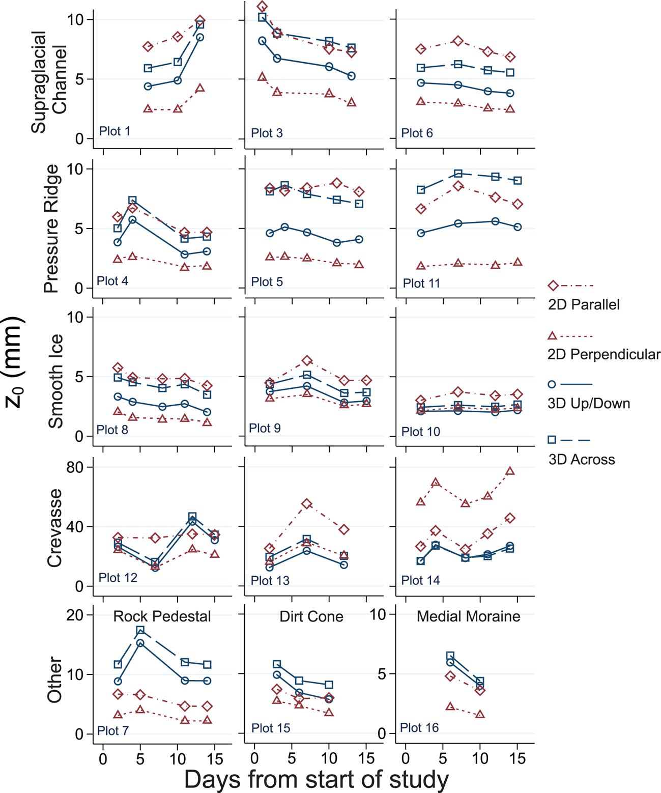
Temporal change of z 0 for plots with multiple surveys. Each row displays a different surface type. Axes scales are variable to allow for a clearer display of temporal trends for Crevasse and Other sites.
Mean z 0 estimates by plot type, wind direction and estimation method

Individual plot measurements are displayed in Figure 6. The standard deviation of values is provided in square brackets.
ANOVA and Kruskal–Wallis tests were used to assess whether differences between the average values over ice facies are statistically significant. The z 0 values exhibited by Crevasse plots are distinct from the other ice facies (Fisher test p < 0.001). While Smooth Ice plots are characterised by lower values of z 0, this difference was only statistically significant when using the 3-D cross-wind estimates (Fisher test p < 0.05). z 0 estimates for Supraglacial Channel plots and Pressure Ridge plots were not distinct (Fig. 5).
3.2 Temporal variability in plot-scale z 0
The z 0 values for the repeat surveys of each plot are displayed in Figure 6. Typically, the evolution of 2-D and 3-D z 0 estimates followed the same trajectory. The z 0 values for all surface types at Hintereisferner were highly dynamic; yet, no clear trend was present over the observation period. Furthermore, no consistent response by surface type was observed.
The Supraglacial Channel plots (1, 3 and 6) displayed two distinctive trajectories: plot 1 exhibited a pronounced increase in z 0 which became more rapid between days 10 and 13, whereas plot 3 and plot 6 z 0 steadily decreased over the same period. Likewise, no consistent trajectory of z 0 was observed for the Pressure Ridge plots (4, 5 and 11): plot 4 demonstrated the highest temporal variability, with an initially rapid increase between days 2 and 4 followed by a sharp decline until day 11, and plots 5 and 11 showed only modest changes throughout the study period. Considering the Smooth Ice plots (8, 9 and 10), plot 8 displayed a gentle decline in z 0 across the observation period, whereas at plot 9 z 0 initially increased then decreased to a value similar to the starting value, and finally plot 10 provided a different evolution again, with z 0 increasing very gradually over the survey period, though changes at this plot were very small.
The observed changes in z 0 estimates for Crevasse plots (12, 13 and 14) were more extreme with changes occurring at rates of >5.0 mm d−1. These results are most likely to reflect difficulties in consistently data modelling the complex terrain present at Crevasse plots. Both the Dirt Cone (15) and Dirty Ice (16) plots showed a clear decrease in z 0 over the field campaign indicating a surface smoothing. The Rock Pedestal plot (7) displayed two different trends: the 2-D z 0 exhibited a gentle decline through the survey period, while the 3-D z 0 value showed greater variability with an initial rapid rise in z 0 followed by a decline back to the original value.
3.3 Distributed z 0 estimates at the glacier scale
TLS survey point density for the lower and upper glacier was ~15 and 20 points m−2, respectively (Fig. 7a). Ice facies exhibited similar relative values for both TLS σ d and SfM derived z 0 estimates (cf. Fig. 5 and Fig. 7). An ANOVA test indicated a statistically significant difference between the groups, while post-hoc Fisher tests showed that Crevasse plots were statistically significantly different from all other plots (p < 0.001) and Smooth Ice plots were significantly different from Supraglacial Channels (p = 0.002). Though not statistically significant (p = 0.051), a difference also appears to exist between TLS σ d values for Smooth Ice and Pressure Ridge plots.
(a) Glacier-wide TLS σ d from 3 August with inset distributions for each ice surface facies (groupings from Fisher pairwise comparisons are displayed above boxes). (b) Linear regressions for 2-D and (c) 3-D estimates of z 0.

Linear regression between TLS σ d and both 2-D and 3-D SfM plot-scale z 0 estimates showed a reasonable fit (r 2 = 0.49 and 0.64, respectively) (Fig. 7c) and were used to produce glacier-scale distributed maps of z 0. Validation of the relationships using withheld data points is presented in Table 3. TLS-based estimates were particularly accurate for Supraglacial Channel, Pressure Ridge and Smooth Ice surfaces with values falling within 1 mm of SfM values. They performed less well for Rock Pedestal and Crevasse plots which were not used to inform the regression relationships.
Comparison of TLS z 0 predictions and SfM z 0 estimates for plots withheld from regression analysis

Spatially distributed maps of TLS-estimated z 0 are displayed in Figure 8. The highest predicted values of z 0 (typically >20 mm) were located towards the margins of the glacier and in its upper reaches where the presence of crevasses led to locally high values of z 0. However, these values were most uncertain given that the regression relationships on which they are based did not perform well for these facies (Table 3). The lowest values of z 0 (0–4 mm) were located in areas of the upper glacier where snow cover was present and towards the centre of the upper glacier scan where Smooth Ice plots were surveyed. Such low values of z 0 were much less common at the lower glacier where the majority of the surface was characterised by z 0 > 4 mm. Maps created from both 2-D and 3-D relationships show a high level of spatial variation in z 0 over Hintereisferner; however, the use of the 3-D z 0 relationship predicted a larger range of values in z 0 arising from the higher gradient term in the linear regression relationship. For example, on the 16 August, the range in 2-D-derived z 0 estimates was 56.45 mm compared to 106.35 mm for 3-D-derived estimates.
Map of estimated 3-D z 0 for the 3rd (a) and 16th (b) day of study, and change in z 0 between the two dates (c). Frequency distributions for each map are inset. See online Supplementary Fig. S2 for equivalent figures for 2-D z 0. Example imagery (d–i) from the field of the different facies observed within close proximity of the areas indicated by letters in (a). Mean, median and standard deviation of glacier-scale TLS derived z 0 estimates (j).

In contrast to plot-scale trajectories, a gradual and consistent increase in TLS derived z 0 estimates was observed for both the mean glacier 2-D (0.05 mm d−1) and 3-D (0.10 mm d−1) estimates (Fig. 8), though glacier-scale median values exhibit a notably slower increase. Between 3 August and 16 August, z 0 estimates over Hintereisferner changed markedly in a number of areas (Fig. 8a–c). Over the crevasses at the true left margin of the glacier and in its upper reaches z 0 can be seen to increase considerably. The smooth surfaces characterised by low z 0 that surround the crevasses in the upper reaches also appeared to increase in roughness, as did the true left margin of the lower glacier. The use of a geographical coordinate system defining the TLS survey cell extents means that the down-glacier progression of surface features during the field campaign may result in local increases and decreases in roughness as features pass from cell to cell. However, the 10 m cell size means that such an effect would be limited over these time scales and this localised variability has no impact on the glacier-scale changes reported above.
The space-for-time substitution lends further support to the notion of a progressive increase in z 0 (Fig. 9). Dated snow lines, areas of the glacier surfaces classified by exposure date and histograms of TLS z 0 estimates within each section are presented in Figure 9. Ice exposed for <2 weeks had a mean and median z 0 value of less than half of ice exposed for >8 weeks. The rate of increase was ~0.07 mm d−1 and appears to be relatively constant for mean values. The rate of increase in z 0 was more variable in median values, with the greatest rates of change occurring between 25 and 37 d of exposure.
(a) and (b) Digitised snow lines from time lapse cameras for upper and lower glacier, respectively. Imagery from www.foto-webcam.eu. (c) Polygons classifying glacier ice areas into zones of exposure length. (d) 3-D TLS z 0 estimates for each classified exposure zone. Estimates are made using the 3 August TLS survey. (e) Mean and median values of z 0 for areas of ice exposed to ablation for varying lengths of time.

Rates of change for each of the classified exposure zones were also calculated for the study period, by differencing z 0 values from the repeat TLS scans from the 3 and 16 August (Table 4). Zones which had been exposed most recently (i.e. farthest up-glacier) experienced the greatest increases in z 0 (1.46 mm). In zones that had been exposed for longer, the ice surface displayed smaller changes until >36 d (for both methods) when changes started to stabilise.
Mean change in 3-D z 0 over the period 3–16 August of classified exposure zones

Standard deviation is in square brackets. See online Supplementary Table S2 for 2-D z 0 changes.
4. Discussion
4.1 Estimating z 0 from microtopographic data
The successful generation of dense point clouds for multiple surface types over Hintereisferner attests to the already recognised potential of SfM for generating microtopographic data for glacial surfaces (e.g. Irvine-Fynn and others, Reference Irvine-Fynn, Sanz-Ablanedo, Rutter, Smith and Chandler2014; Chambers and others, Reference Chambers2019). However, the application of SfM was most challenging over Crevasse plots and over Rock Pedestal plots; gaps in the point clouds within the deep vertical crevasse walls and steep faces of rock pedestals were observed and are likely to be a consequence of imperfect image capture (given safety concerns) and unavoidable shadowing. While caution is required when interpreting microtopographically-derived z 0 values over such surfaces, this impact is limited for upscaling owing to their relatively small area at the glacier scale.
2-D and 3-D z 0 estimation methods displayed differing levels of agreement for different surface types. For surfaces devoid of large protruding roughness elements, the methods give similar results; where such roughness elements were present, there was less agreement between the two methods. Over Dirt Cone and Rock Pedestal plots 3-D z 0 estimates were typically greater than their 2-D counterparts. These findings corroborate those of Smith and others (Reference Smith2016) over Kårsaglaciären in northern Sweden and Quincey and others (Reference Quincey2017) who observed that for debris-covered ice in the Himalaya, with z 0 ≫ 5 mm, 3-D estimates of z 0 far exceeded 2-D estimates. Conversely, at Crevasse plots, 2-D z 0 estimates were larger than the 3-D estimates, as also observed by Smith and others (Reference Smith2016).
The difference in 2-D and 3-D z 0 estimates for different surface types most likely arises from the different way in which each method calculates frontal area. The 3-D method partially accounts for sheltering by ignoring all roughness elements below the detrended plane; the influence of this calculation step was most pronounced for Crevasse plots which contained extremely deep negative extensions below this plane. In contrast, the 2-D method included every point within a given transect and thus incorporated the effect of the deep crevasse as far as it was surveyed. As such, the 2-D method would generate the same value for an inverted crevasse transect as a regular crevasse. The approach of the 3-D method and its account for sheltering, therefore, seems reasonable given that a roughness element extending positively above the surface will likely impede the flow of air considerably more than a roughness element of the same size extending below the surface. Therefore, for plots with large roughness elements that extend above the detrended plane (e.g. Rock Pedestal and Dirt Cone) 3-D estimates exceed 2-D estimates and where roughness elements extended negatively below the detrended plane (e.g. Crevasses) 2-D estimates exceed 3-D estimates. Overall, the more sophisticated representation of sheltering possible and the increased availability of topographic data sufficient for 3-D z 0 estimates indicates that 3-D topographic methods will likely provide the source of z 0 values for use in distributed melt models.
4.2 Plot-scale z 0 variability at Hintereisferner
The lowest values of z 0 recorded over Hintereisferner were between 1 and 5 mm for Smooth Ice, Dirty Ice and Compound surface types. These z 0 values are greater than some estimates of z 0, which for particularly smooth ice surfaces can be <1 mm (e.g. Grainger and Lister, Reference Grainger and Lister1966; Arnold and Rees, Reference Arnold and Rees2003; Giesen and others, Reference Giesen, Andreassen, van den Broeke and Oerlemans2009); yet, the values seem reasonable given that even the smoothest surfaces observed were visibly degraded and exhibited topographic variability. Indeed, the range of z 0 values observed over Hintereisferner compares more favourably with degraded and melting glacial ice surfaces in the literature (e.g. Greuell and Smeets, Reference Greuell and Smeets2001; Sun and others, Reference Sun2014; Guo and others, Reference Guo2018). Pressure Ridge and Supraglacial Channel plots exhibited elongated roughness elements with z 0 ranging between 3 and 10 mm; estimates within the literature of z 0 over elongated glacier ice hummocks range between 0.7 and 6.9 mm (e.g. Munro, Reference Munro1989; Fitzpatrick and others, Reference Fitzpatrick, Radić and Menounos2019), suggesting the values presented here are robust. Estimates of z 0 for Rock Pedestal and/or Dirt Cone plots have hitherto not been made; however, given the scale of roughness elements the larger estimates of z 0 of >10 mm predicted by 3-D methods seem reasonable. The most topographically variable surfaces over Hintereisferner were present at Crevasse plots, as reflected in high z 0 estimates for both 2-D and 3-D methods which are typically >20 mm. Smith and others (Reference Smith2016) recorded similarly large values over crevassed plots at Kårsaglaciären, while over very rough ice surfaces comparable values have been recorded (e.g. Obleitner, Reference Obleitner2000; Smeets and van den Broeke, Reference Smeets and van den Broeke2008; Azam and others, Reference Azam2014).
Notably, our estimates of z 0 over Hintereisferner are typically larger than those obtained from similar studies utilising SfM imagery over bare ice surfaces (e.g. Irvine-Fynn and others, Reference Irvine-Fynn, Sanz-Ablanedo, Rutter, Smith and Chandler2014; Smith and others, Reference Smith2016). These higher z 0 values are likely a function of scale; the 10 m × 10 m plots utilised in this study are ~25× greater in area compared to the 2 m × 2 m plots utilised in these previous applications of the 2-D and 3-D z 0 estimation methods. Microtopographic estimations of z 0 have been found to show scale dependence, with z 0 increasing with plot size (Chambers and others, Reference Chambers2019). Therefore, when compared to the z 0 estimates of Irvine-Fynn and others (Reference Irvine-Fynn, Sanz-Ablanedo, Rutter, Smith and Chandler2014) and Smith and others (Reference Smith2016), higher values of z 0 for a similar surface should be expected. We assume herein that, despite this recognised scale dependence of z 0 values, their temporal evolution is relatively consistent within the length scale ranges of these plot-focused studies.
4.3 Upscaling z 0 estimates using TLS surveys
An assessment of the TLS z 0 estimates over a variety of different ice facies is presented in Figure 8. The map correctly identifies high and low values of z 0 for the steep ice exposures that contained crevasses and the smooth snow surfaces, respectively (d). Areas of the glacier with smooth ice surfaces and pressure ridges (f) are characterised by a z 0 ranging from ~2 to 7.5 mm throughout the upper glacier. Crevasses towards the edges of the glacier are particularly well highlighted (e) and are represented by z 0 values generally >12.5 mm and in some cases >50 mm. Relatively small, yet extreme, topographic features are also highlighted by high values of z 0 such as an area containing extensive debris cover, large rock pedestals (h), a large moulin (i) and the deep supraglacial channel network feeding it in the centre of the upper glacier. Due to a longer exposure of the ice surface, values of z 0 (ranging between 4 and 12.5 mm) over the lower glacier were typically greater than those over the upper glacier, characterising the topographic variability of the extensive network of supraglacial channels and hummocky ice present (g).
Surface roughness measured from the TLS surveys exhibited a stronger relationship with SfM estimated z 0 values than those achieved previously (e.g. Smith and others, Reference Smith2016). This was potentially due to the larger plot size used over Hintereisferner, allowing for TLS scans to better reflect topographic variability when compared to the 2 m × 2 m plots studied by Smith and others (Reference Smith2016). The utility of TLS σ d as a proxy for z 0 was further demonstrated by the finding that TLS σ d values for separate ice facies fall into distributions similar to more detailed plot-scale z 0 estimates. The maps of z 0 estimates derived from TLS data facilitate clear visualisation of the variability of z 0 across Hintereisferner. Previous z 0 maps over bare ice surfaces have typically represented spatial variability by extrapolating point data (e.g. Brock and others, Reference Brock, Willis and Sharp2006). The maps presented here offer a step forward and could be readily applied in distributed melt SEB models. It should be noted, however, that model performance was weaker over Crevasse plots, especially for 2-D estimates, though this is perhaps related to the sheltering and SfM model quality issues mentioned above. Certainly, the approach demonstrated herein provides a more robust representation of z 0 than a constant value, as adopted by some SEB models (e.g. van As, Reference van As2011; Fausto and others, Reference Fausto, van As, Box, Colgan and Langen2016b).
4.4 A scale-dependent model of the temporal variability of z 0
Several studies have reported considerable variation in z 0 over the course of an ablation season (e.g. Guo and others, Reference Guo2011; Sicart and others, Reference Sicart, Litt, Helgason, Tahar and Chaperon2014; Fitzpatrick and others, Reference Fitzpatrick, Radić and Menounos2019). Much of this variability is accounted for by differences in both wind speed and direction; however, the development of surface microtopography through time also has a significant effect. The effect of evolving topography on z 0 is to date relatively poorly understood and the literature shows multiple contrasting trends in the evolution of z 0 through time (e.g. Smeets and others, Reference Smeets, Duynkerke and Vugts1999; Smeets and van den Broeke, Reference Smeets and van den Broeke2008; Smith and others, Reference Smith2016). In an effort to unify these different perspectives, we adapted the three-stage model of Guo and others (Reference Guo2011) to propose a new scale-dependent theoretical model for predicting the evolution of z 0 throughout an ablation season.
Our model separates the temporal z 0 evolution model of Guo and others (Reference Guo2011) into five stages (Fig. 10a). Stage 1 details the transition of the surface from fresh snow cover, to a mixed snow and ice surface, at which z 0 reaches its first peak (as per Guo and others, Reference Guo2011). Stage 2 maps the transition of the surface from this mixed cover to a bare ice surface and can take several trajectories depending on the roughness of the underlying ice surface (the suggested range of which is noted as grey dashed lines in Fig. 10a). Guo and others (Reference Guo2011) observed a decreasing z 0 as a flat ice surface was gradually exposed; conversely Smeets and van den Brooke (Reference Smeets and van den Broeke2008) noted an increase in z 0 at this stage at the Greenland ice sheet as ice hummocks were exposed. No observations were made of these two stages at Hintereisferner; however, the relatively rough underlying ice observed in the field indicates that a substantial decrease in z 0 during stage 2 is unlikely. Our field observations begin at stage 3 which represents a period of time between ice exposure and the clear development of surface features, during which only small channels are present in the surface and ice hummocks are yet to develop. In stage 4 z 0 rapidly increases, as surface features are established and are pronounced by increasing melt rates and the development of a complex meltwater channel network. During stage 5, z 0 approaches its peak value beyond which the density of some smaller-scale roughness elements will reach values where wake-interference and skimming flow are initiated thereby decreasing z 0.
(a) Initial, five-stage theoretical model for z 0 development during the ablation season (developed from Guo and others (Reference Guo2011) where stages 2–4 were grouped together). Temporal evolution of the ice facies observed over Hintereisferner is also indicated (excluding Compound, Rock Pedestal and Crevasse plots). (b) Proposed scale-dependent theoretical models with indications of where observed changes to each exposure zone over study duration would fall on model, based on field observation.

To inform the development of the theoretical model, each plot (excluding Rock Pedestal and Crevasse plots) was placed on the proposed model and a simplification of the z 0 trajectory indicated (Fig. 10b). Following the space-for-time substitution in Figure 9, plots located towards the lower end of the glacier, over which the ice surface had been exposed for a longer time period, appear further along the transition model. Field observations of the ice surface were used to guide the overall positioning along the theoretical curve. The trajectory of z 0 values within the plots rarely followed the anticipated trajectory. Indeed, the theoretical model predicts an increasing value of z 0; contrastingly, plot-scale z 0 estimates showed highly variable trajectories with an overall decrease in z 0 for the majority of plots, despite the existence of pronounced surface features. Two of the Smooth Ice (P8 and P9) plots, which would be expected to be characterised by a relatively constant z 0, demonstrated a variable value of z 0 which decreased over the course of observation. Overall, only three plots (P10, P11 and P1) exhibited the expected evolution of z 0 anticipated from the model.
Here we argue that scale plays an important role in determining how the temporal evolution of z 0 is observed. At the plot scale, the complex interaction of preferential melt and meltwater channel development controls the microtopography of the surface at Hintereisferner. The simple model proposed in Figure 10a is certainly inadequate and cannot represent the variability of z 0 due to these processes. The variability in the trajectory of z 0 is high and is unlikely to reveal any underlying progressive evolution of z 0 ice surfaces except over long time periods. Plot-scale trajectories of z 0 appear to be relatively unpredictable and independent of the ice facies, contrasting the findings of Smith and others (Reference Smith2016). Other studies suggest that the diversity of plot-scale z 0 trajectories is most pronounced following the initial melt of the snow surface. At the plot scale, Fitzpatrick and others (Reference Fitzpatrick, Radić and Menounos2019) measured z 0 over the course of an entire ablation season using sonic anemometers and observed an initial rise in z 0 as snow cover melts to form sun cups, supporting the underlying plot-scale evolution of z 0. Following the initial rise, they recorded a period of 60 d with no trend in z 0, potentially reflecting the relatively stable behaviour of z 0 through late stage 2 to early stage 4. Similarly, Brock and others (Reference Brock, Willis and Sharp2006) recorded wind profile and microtopographic estimations of z 0 across the course of the 1993 and 1994 ablation seasons of Haut Glacier D'Arolla, Switzerland. Although their z 0 observations over snow surfaces support the progression proposed in stage 1, they observed a number of different temporal trends in the evolution of z 0 values over exposed ice surfaces, including a declining value of z 0 towards the end of the ablation season.
The underlying progression of z 0 can only be revealed through observations of greater spatial scales, over which the unpredictable behaviour of individual plot values are aggregated into a more predictable trajectory. Figure 10b presents a visual representation of this theoretical z 0 evolution model. At the glacier scale, TLS derived z 0 estimates display a constant and relatively linear increase in mean z 0 at a rate of ~0.10 mm d−1, over the 15 d observation period (Fig. 10b). The space-for-time substitution of Figure 9 lends further support to the notion of a progressive increase in z 0 over a 50 d period, with a slightly slower increase in the mean z 0 of ~0.07 mm d−1. Observed changes in z 0 within exposure zones (Table 4) indicate a more-or-less linear increase during the study period. While older exposed surfaces experience smaller increases than more recently exposed surfaces, the reduction in gradient is not as pronounced as suggested in the underlying theoretical model. This theoretical glacier-scale behaviour is supported by the spatially distributed maps of z 0 presented in Brock and others (Reference Brock, Willis and Sharp2006), who over six periods throughout the melt season, observed a clear increase in glacier-scale z 0 with the onset of melt, continuing until snowfall at the end of the ablation season, at which point a lowering of z 0 is observed at a number of sites.
4.5 Further work
Both 2-D and 3-D z 0 estimates have been demonstrated to reasonably approximate aerodynamically derived z 0 values (Quincey and others, Reference Quincey2017; Chambers and others, Reference Chambers2019); yet, further consideration of the drag coefficient (Quincey and others, Reference Quincey2017), the influence of sheltering effects and scale dependencies of microtopographically derived z 0 would give estimates a stronger theoretical foundation.
The proposed scale-dependent trajectories of z 0 outlined in Figure 10 infers the behaviour of z 0 over an entire ablation season. Yet, plot-based estimates of z 0 observed at Hintereisferner had a maximum measurement period of 14 d, with some plots being observed over shorter time periods and glacier-scale TLS-based estimates spanning 13 d only. Although the time period was extended to ~50 d using a space-for-time substitution, the results of which supported a progressive increase in z 0, the conclusions presented herein are limited by the short duration over which observations were made. The space-for-time substitution should be treated with some caution, given the potential for longitudinal glacier interactions, notably the downstream transfer of meltwater, which may influence the signal observed. Certainly, a longer observation period would allow for a clearer assessment of the accuracy of the theoretical model proposed.
Finally, with a larger number of plot-scale observations, a more objective classification of ice surface facies becomes possible, potentially based on observed roughness metrics from glacier-scale surveys. Such distributed maps of ice surface type could then better inform the production of distributed z 0 maps via individual regression relationships for each surface type. The incorporation of such z 0 maps into a distributed SEB model represents the key focus for further research, though there remains the question of how much detail of z 0 variability in both space and time is required to have a substantial impact on turbulent flux estimation.
5. Conclusions
This research adds to a growing literature (e.g. Brock and others, Reference Brock, Willis and Sharp2006; Smeets and van den Broeke and others, Reference Smeets and van den Broeke2008; Guo and others, Reference Guo2011; Smith and others, Reference Smith2016; Quincey and others, Reference Quincey2017; Fitzpatrick and others, Reference Fitzpatrick, Radić and Menounos2019) that emphasises the need to more comprehensively represent z 0 in SEB models to reduce errors in estimates of ablation. Specifically, the assumption of a constant z 0 value over ice surfaces, commonly 1 mm (e.g. van As, Reference van As2011), requires improvement. Representing z 0 more accurately in SEB models is especially important given the increasing contribution of turbulent fluxes to glacier SEB as the climate becomes wetter, windier and warmer.
The recent proliferation of high-resolution topographic data acquisition techniques has advanced the potential for estimations of z 0 and enabled effective relationships to be developed to upscale plot results to the glacier scale. The use of 3-D methods to estimate z 0 makes the best use of this available data. Plot scale estimates of z 0 demonstrated substantial variability in both space and time, ranging from z 0 < 3 mm to z 0 > 40 mm. z 0 over such surfaces can change at rates in excess of 0.25 mm d−1 as the surface melts and can be due to complex interactions between meltwater channel development and preferential melt. At the glacier scale, spatial variability in z 0 values was >2 orders of magnitude but a consistent increase in z 0 of 0.07–0.10 mm d−1 was observed.
Our findings indicate that glacier scale topographic datasets can usefully capture the variability in ice surface roughness that is relevant for the estimation of z 0. While a TLS was available for this study, airborne laser scanning or even satellite-derived datasets that are more widely available may provide sufficient topographic information to estimate z 0 variability in space and time to the extent that is required by distributed melt models.
Overall, we contend that by interpreting the temporal trends in z 0 as a function of the spatial scale over which they are observed, our theoretical z 0 model goes some way towards unifying a variety of contrasting temporal trends observed within the wider literature. The interpretation presented here is that plot scale trends in z 0 are stochastic in the short term but by extending either the length of observation or the spatial scale underlying trends in z 0 are revealed. Further work into theoretical scale-dependent behaviour of z 0 through time is required. If such work supports a progressive increase in z 0, constraining the rate of this increase may pave the way for representation of the temporal development of z 0 in SEB models.
Supplementary material
The supplementary material for this article can be found at https://doi.org/10.1017/jog.2020.56
Acknowledgements
Fieldwork was funded by an INTERACT transnational access grant awarded to MWS under the European Union H2020 Grant Agreement No. 730938. The TLS facility is financed by the University of Innsbruck and jointly operated by the Department of Geography and the Department of Atmospheric and Cryospheric Research. JRC is supported by a NERC PhD studentship (NE/L002574/1). IS was funded by Austrian Science Fund (FWF) grant T781-N32. The authors acknowledge Matt Westoby and Andy Baird and two anonymous reviewers for constructive comments on this work. The authors declare that they have no conflicts of interest.


 Open access