2.1. Observation strategy

The CRAFT fly’s eye observation strategy and data processing pipeline was originally described in detail in Bannister et al. (Reference Bannister2017). Below, the key features are revisited, with some minor updates to the analysis strategy.

CRAFT observations have primarily made use of ASKAP antennas as they became available, with between one and eleven antennas observing simultaneously. Since the beam-formed commensal mode of CRAFT is still being commissioned, antennas have been operating in fly’s eye mode, with data from each antenna analysed independently.

We have been observing using the ‘square6×6’ footprint prior to March 17^th, and the ‘closepack36’ footprint subsequently. The beam patterns of these footprints are shown in Figure 1. While the overlapping beams reduce the total effective survey area for the closepack36 configuration, they also reduce the importance of sidelobes in rate calculations and increase the likelihood of a multibeam detection. The process for forming ASKAP beams is described in McConnell et al. (Reference McConnell2016); this results in minor variations in beam fidelity every time beamforming is performed, while minor variations in gain and phase from each digital receiver port will vary the beamshape with time once beamforming has been performed.

Observations have used a contiguous bandwidth, from 1 128 to 1 464 MHz, dividing into 336 1-MHz channels.Footnote ^a To reduce the data rate to computationally feasible levels, the squared complex voltages from both polarisations are integrated over 1 500 samples, i.e. 1.2656 ms at ASKAP’s 32/27 oversampled rate. This causes dispersion smearing within a channel to exceed the integration time at a DM of 333 pc cm⁻³ at band centre.

These data are then recorded to disc, and searched for FRBs as described below.

2.2. Data processing and analysis

CRAFT FRB searches are performed in near-real-time by ‘FREDDA’, a GPU-implementation of the FDMT algorithm (Zackay & Ofek Reference Zackay and Ofek2017). It also performs basic checks of data fidelity, such as flagging saturated channels, and subtraction of zero-dispersion artefacts. The search space is restricted to dispersions of between 100 and 4 096 samples, corresponding to dispersion measures between 95.9 and 3 930 pc cm⁻³ in approximately 0.959 pc cm⁻³ increments. The final stage in FREDDA searches in pulse width space, using 32 uniform windows over 1, 2, 3,…, 32 1.2656 ms samples, and returns the candidate with the most significant width.

Metadata on all candidates over 7σ significance are reported by FREDDA. These are then passed to a friends-of-friends algorithm (Huchra & Geller Reference Huchra and Geller1982) to merge candidates within two increments in any dimension in search space, i.e. DMs within ±1.92 pc cm⁻³ and arrival times within ±1.53 ms. The most significant candidate in each group is recorded, and since a great number of RFI candidates with widths greater than 16 samples (20.25 ms) were found, these are rejected. Remaining candidates above 9.5σ are visually inspected for final confirmation as FRBs. Candidates from each beam are treated independently, although once an FRB is identified, data from neighbouring beams are used for source localisation. Thus, to a good approximation, the dependency of CRAFT sensitivity on FRB arrival direction can be calculated from the sensitivity envelope of all 36 beams.

The reporting threshold of 7σ for FREDDA candidates was chosen because (a) this allows a measurement of pure noise events (observed up to 8σ); (b) candidates observed above 7σ in two beams can theoretically be excluded as being pure noise events, and identified as FRBs; and (c) the distribution in search-parameter space of reported significance about peak significance will be more peaked for true FRBs, aiding in the exclusion of RFI. We have yet to perform a systematic multibeam search as described by (b), with only FRB 171216 being coincidentally discovered in this manner (Shannon et al. Reference Shannon2018), while (c) was not required for exclusion of RFI.

Figure 2.

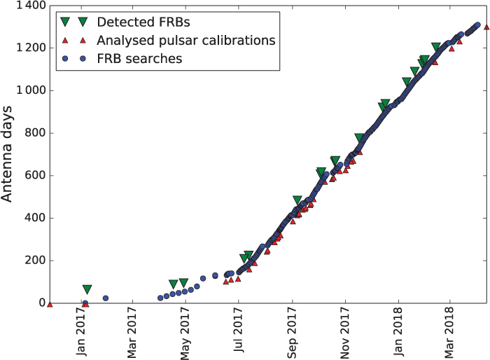
Timing of pulsar calibration runs (red triangles) compared to detected FRB times (green inverted triangles) reported in Shannon et al. (Reference Shannon2018), and the cumulative FRB search observation time in antenna-days (blue dots). No antenna efficiency factors have been included.

3.1. Fitting method

Data from 38 pulsar calibration observations taking during the survey have been analysed. This included all such observations up to November 2017, at which point the observing configuration and fluctuations in sensitivity (see Section 3.3) had stabilised.

The calibration data were processed through FREDDA and friends-of-friends using exactly the same algorithms as for FRB searches, with the exception that candidates down to a DM of 46 pc cm⁻³ are included. Candidates with DMs within ±4 pc cm⁻³ of the known values of the target pulsar (67.99 pc cm⁻³ for B0833-45 and 478.8 pc cm⁻³ for B1641-45) (Manchester et al. Reference Manchester, Hobbs, Teoh and Hobbs2005) from the on-pulsar beam only are selected. All such candidates from a given calibration observation are binned in terms of their measured signal-to-noise values as determined by FREDDA, σ_F. The estimated fraction of coincidental triggers contaminating this sample is less than 0.1%, as is the loss from pulses with misestimated DMs falling outside the DM search range.

Figure 3.

Examples of a fits to a pulsar calibration observation, for B0833-45 (left) and B1641-45 (right). Points: histogram of detected pulses from B1641 in a single beam, showing Poisson error bars; line: fit from equation (1).

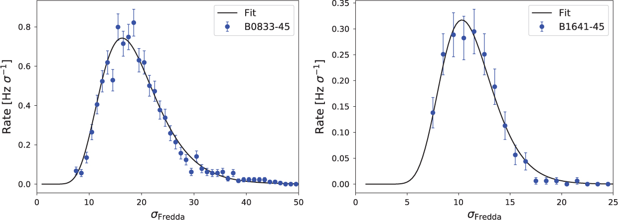
For each beam/antenna/calibration, histograms of σ_F are normalised to the observation time, producing a rate histogram R. The rate is then fitted using a log-normal distribution, which has been found to well-model the pulse amplitude distribution of both B1641-45 (Cairns, Johnston, & Das Reference Cairns, Johnston and Das2004) and B0833-45 (Cairns, Johnston, & Das Reference Cairns, Johnston and Das2001):

(1) \begin{equation}R(\sigma_{\rm F}) = \frac{r}{\Delta \sigma_{\rm F} \sqrt{2 \pi}} \exp\! \left( - \frac{(\log_{10} \sigma_{\rm F} - \mu)^2}{2 (\Delta \sigma_{\rm F})^2} \right).\end{equation}

Here, r measures the total fitted rate of pulses (both above and below the CRAFT detection threshold), μ is log₁₀ of the characteristic sensitivity, and Δσ_F is the spread. The analysis of Cairns et al. (Reference Cairns, Johnston and Das2004) applies to each time-resolved portion of the pulse profile, at a resolution much smaller than Δt = 1.2656 ms. However, the reported values of the fitted parameters change only slowly over the pulse profile, so we expect it to be sufficiently applicable.Footnote ^b

The fit procedure uses the Levenberg–Marquardt algorithm, implemented in Python 2.7.14 via the SciPy 1.0.0 function scipy.optimize.curve_fit (Jones et al. Reference Jones2001). A bias towards low values of efficiency was found when using Poisson-weighted errors, so all errors were set to unity. Histograms are then multiplied with the bin width in log-space, and divided by the observation time to obtain units of rate per log-interval in σ_F. An example of a fit is given in Figure 3.

When sensitivity is low, only the falling tail of the pulse distribution is observed, and the fit becomes degenerate. To remove this, fits were first performed to estimate Δσ_F, and then data were re-fitted leaving only r and μ free. The correlation of fit errors was typically less than 2%, and slightly anti-correlated. This amounts to modelling a constant underlying distribution of pulse strengths for each pulsar, which are then are modified independently by efficiency and sensitivity.

3.2. Efficiency

Bursts of RFI, large power spikes, or simply a malfunction in the hardware during the commissioning phase can cause a loss of effective observing time, T _eff, compared to the total observation time, T _obs. The observation efficiency ϵ is thus defined as

(2) \begin{align}\epsilon \equiv \frac{T_{\rm eff}}{T_{\rm obs}}\end{align}

and can be measured through pulsar calibration observations comparing the fitted pulsar pulse rate, r, to the known spin rate r ₀, taken from PSRCATFootnote ^c (Manchester et al. Reference Manchester, Hobbs, Teoh and Hobbs2005):

(3) \begin{align}\epsilon = \frac{r}{r_0}.\end{align}

This assumes that factors leading to a loss of T _eff affect both pulsar and FRB searches equally. Note that the fitted value of r reflects the total pulsar rate, i.e. it accounts for missed below-threshold pulses.

Figure 4.

Normalised histograms of efficiency for calibration observations of the pulsars B1641-45 and B0833-45, calculated relative to base rates r ₀ of 2.1975 and 11.195 Hz, respectively (Manchester et al. Reference Manchester, Hobbs, Teoh and Hobbs2005). The data are composed of 9 710 independent measurements, and Poissonian errors are too small to be shown on the plot.

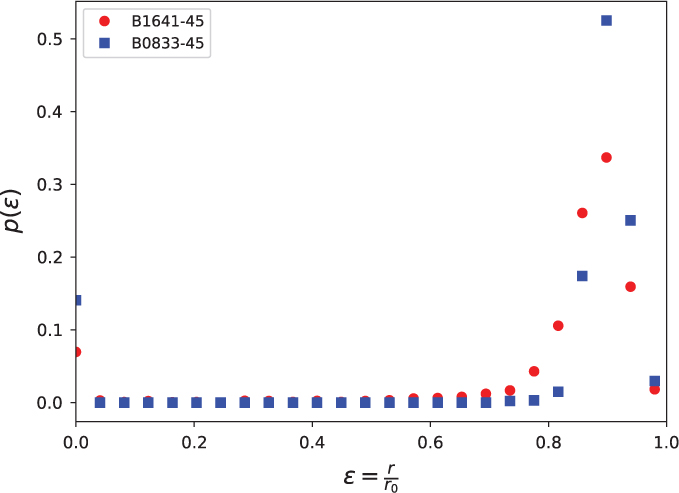
Histograms of the fitted rate are given in Figure 4 for both B1641-45 and B0833-45. In general, CRAFT efficiencies are in the 80–95% range. The 6–7% (85–100 antenna-days equivalent) of data at zero efficiency is partly due to beam 35 producing unusable data, and partly due to miscellaneous faults during commissioning observations.

The efficiencies measured with B1641-45, ϵ _B1641, peak at a similar value (90%) to those measured with B0833-45, ϵ _B0833. However, they have a slight tail at lower efficiencies. Since the fitted efficiencies are almost uncorrelated with signal strength, it seems this is unlikely to be due to Vela (B0833-45) being much stronger than B1641-45. While the exact cause of this is unknown, it may be due to different data-taking conditions and antenna performances during calibration runs with each. For instance, most of the data used in this study come from the second half of 2017, when B0833-45 was more visible during nighttime. Furthermore, chirped RFI pulses were present in some ASKAP data, and may have been responsible for some of the variation in efficiency.Footnote ^d An alternative is that Vela is almost 100% linearly polarised, so that gain offsets between X and Y polarisations would affect the two pulsars differently.

Excluding the values at 0 (the loss of beam 35 is accounted for in Section 4, while the zero-valued data are treated in Section 3.5), fits to antenna and beam dependence did not produce statistically significant results, and fitted mean efficiencies varied within ±2%. No dependency on power fluctuations (see Section 3.3) was observed. Hence, a global mean value of efficiency, $\overline{\epsilon}$ , is calculated by averaging results over both pulsars, finding $\overline{\epsilon}=0.87$ .

Figure 5.

Example of power fluctuations in ASKAP commissioning data. Top: example time series of DM0 power p(t), showing the fluctuations over a limited time range. Bottom: Fourier transform magnitude of the time series, taken over 4 096 samples. The strength of the peak near 300 Hz is denoted p ₃₀₀. The other peaks are aliased multiples of 300 Hz.

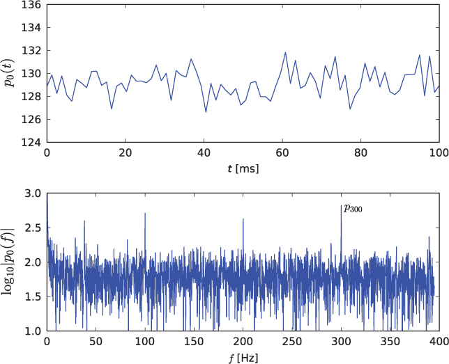
3.3. Power fluctuations

The only anomaly identified in ASKAP commissioning data was the presence of systematic fluctuations in the digitised CRAFT voltages on timescales of ms and greater. The fluctuations affected all frequency channels uniformly, but grew stronger with increased electrical power requirements, i.e. cooling, during daylight hours. It also varied systematically both over the elements of each PAF, and between antennas, according to the power distribution network.

An example of data affected by power fluctuations is given in Figure 5, showing the systematic effect when summed over all channels [‘DM0’ power, p ₀(t)], and a discrete Fourier transform (DFT) of the DM0 signal, p ₀(f). A strong peak at 300 Hz is clearly present, with secondary peaks corresponding to aliased multiples of 300 Hz.

The cause of the problem has now been identified as large voltage fluctuations in the PAF power supplies, which has been fixed by adjusting supply voltages. However, 2 months of CRAFT data (from late June to August 2017) were affected. This coincides with the dearth of FRBs from mid-July to August 2017, with no FRBs observed during 280 antenna-days. Equal or longer waiting times occur with a probability of approximately 1%; given we sample 19 such waiting times, this observation is not significant, even before accounting for sensitivity reductions, which we do below.

Without modifying the search algorithm, power fluctuations are expected to decrease sensitivity by increasing the system equivalent flux density (SEFD), and hence the nominal detection threshold. It was expected that most of the original sensitivity could be recovered in offline analysis, either by removing the main Fourier components or by subtracting the systematic p ₀(t) signal from the data (DM0 subtraction). Preliminary investigations have found however that both methods produce an equally limited recovery of sensitivity, with a DM0 subtraction method being implemented due to its computational simplicity. This suggests that sensitivity loss is caused at the beamforming stage, by effectively modifying the weights with which PAF elements are summed. The sensitivity loss is therefore deemed unrecoverable—it is parameterised in the next section.

3.4. Modelling sensitivity

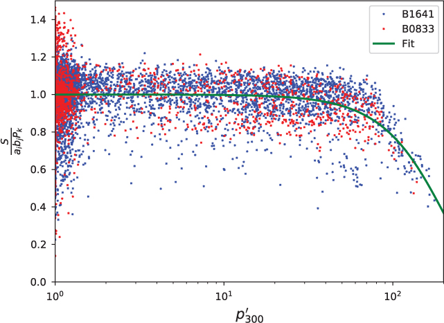
The relative sensitivity s_i,j of CRAFT FRB searches with antenna i and beam j is modelled as follows:

(4) \begin{align}s_{i,j}\left(p^{\prime}_{300}\right) & = a_i b_j P_k n\left(p^{\prime}_{300}\right),\end{align}

(5) \begin{align}n\left(p^{\prime}_{300}\right) & = \left[ \left(\frac{p^{\prime}_{300}}{c_1} \right)^2+1 \right]^{-c_2}\!, \end{align}

(6) \begin{align}p^{\prime}_{300} & = \frac{p_{300}}{p_{\rm med}},\end{align}

where a_i and b_j are the relative sensitivities of antennas i and beam j, P_k is the peak emission of pulsar k, $p_{300}^{\prime}$ and p _med are, respectively, the 300 Hz and median powers illustrated in Figure 5, and c ₁ and c ₂ are scaling constants. The b_j for each of the two footprints were treated as independent variables, due to their differing sky positions (Figure 1). The functional form of n was found empirically, with $p^{\prime}_{300}$ being normalised by the median power p _med giving the best fit.Footnote ^e

For the 19 antennas and two footprints used in the search so far, this gave a 93-parameter fit, after constraining the sensitivities of antenna 8 and beam 20 (one of the central beams in closepack36 configuration) to unity, i.e. a ₈ = b ₂₀ = 1. The fit procedure, as in Section 3.1, also uses the implementation in Python’s scipy.optimize.curve_fit function.

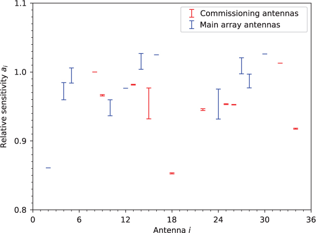
Fit errors were estimated with a bootstrapping technique. Pulsar calibration observations were removed one at a time, and used to re-estimate the fit parameters. Since slightly less data are being used in each fit, the resulting variation is too large by a factor of [n _cal/(n _cal − 1)]^0.5, where n _cal is the number of calibration observations in which each antenna participated. Some antennas (02, 12, 16, and 30) were only involved in one calibration observation, and hence errors could not be estimated. By definition, however, these antennas contributed very little to observations, and hence this does not greatly affect the average sensitivity.

Figure 6.

Fitted sensitivities a_i for each antenna i, relative to antenna 08. No errors could be fitted for antennas 02, 12, 16, 30, and 32, which participated in only a single calibration observation, while main array antennas, and antenna 15, participated in few, leading to larger uncertainty.

Figure 7.

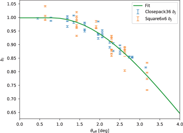
Points: relative beam sensitivities b_i from the fit to equation (4). Line: fit of beam sensitivity as a function of the angular offset θ _off from the antenna optical axis. Main array antennas (blue) have already been commissioned, and are connected to the ASKAP correlator; commissioning antennas are those used during the commissioning period.

Figure 8.

The effect of 300 Hz noise on CRAFT sensitivity. Points: calibration observations of B1641 (blue) and B0833 (red), after removing the fitted effects of antenna, beam, and pulsar single pulse detection significance [equation (4)], compared to the fitted noise function n [equation (5)].

3.4.1. Results of the fit

The fitted values of a_i , b_j , and $n(p_{300}^{\prime})$ are illustrated in Figures 6–8, respectively. The median significances at which single pulses from each pulsar are detected in CRAFT data from antenna 08 beam 20 using FREDDA were found to be P _B1641 = 12.44 ± 0.05 and P _B0833 = 16.87 ± 0.13. The mean antenna sensitivity was found to be 96.7% that of antenna 08, with rms variation between antennas of ±4.7%. This value, calculated on MkII PAFs, compares well with the approximate ±5% variation in T _sys and SEFD found by McConnell, Bannister, and Hotan (Reference McConnell, Bannister and Hotan2017) for a partially overlapping sample of antennas with MkI PAFs.

Beam sensitivities far from the antenna optical axis are expected to fall, due primarily to the finite extent of the PAF. To model this, the values of b_i are fitted as a function of beam angular offset, θ _off, according to a flattened Gaussian:

(7) \begin{eqnarray}b(\theta_{\rm off}) & = & \left\{ \begin{array}{ll}1 & \theta_{\rm off} \le \theta_0 \\e^{-0.5 \left(\frac{\theta_{\rm off}-\theta_0}{\sigma_{\theta}} \right)^2 }& \theta_{\rm off} > \theta_0. \\\end{array}\right.\end{eqnarray}

The results of this fit are shown in Figure 7. The fitted beam sensitivities have also been compared to the apodising function found by McConnell (Reference McConnell2017), which includes the 2D structure of the PAF. This was found to over-correct the beam sensitivities. A possible cause may be that the measured b_j are functions of beam shape, peak sensitivity, and mean pointing error. Since beams far from the optical axis are approximately 5% broader than inner beams, a mis-pointed outer beam will suffer less sensitivity reduction than a mis-pointed inner beam.

From Figure 8, the 300 Hz power fluctuations cause negligible change in sensitivity, up to the point where $p_{300}^{\prime} \approx 50$ , after which the sensitivity falls sharply. The fitted values of c ₁ and c ₂ [equation (5)] are 1.22 × 10⁴ and 3 700 respectively, although these values are poorly constrained, highly correlated, and their errors are not well-estimated with the bootstrap method due to the small amount of data with very high values of $p_{300}^{\prime}$ .

3.5. Integrated sensitivity

The time-integrated sensitivity of the CRAFT GL50 FRB survey is treated as a function of the sensitivity of the telescopes used (the a_i ) and power fluctuations, $n(p_{300}^{\prime})$ ; the fitted values of b_i will be incorporated into the beam model in Section 4.

The relative sensitivity of each antenna relative sensitivity s_i,k for each antenna i and (typically 1 h) scan k is calculated as follows:

(8) \begin{align}s_{i,k} = \frac{a_i}{35} \sum_{j=0}^{34} n\!\left(p_{300,i,j,k}^{\prime}\right)\!,\end{align}

where the $p_{300,i,j,k}^{\prime}$ are calculated using the first 10 × 1 024 samples from each scan. The effect of the virtual loss of beam 35 is accounted for in beamshape estimates (Section 4).

This procedure ignores the fact that power fluctuations do not appear uniformly over the total beam pattern, nor do its effects add linearly between beams. Beams with low sensitivity will be partially compensated for by neighbouring beams, and the effect of an edge beam having its sensitivity reduced will be greater than for an interior beam. However, it has been found that neighbouring beams experience similar amounts of power noise, so these effects will be small, and are ignored.

Figure 9.

Histogram of total observation time at relative sensitivity s, divided into contributions from closepack36 (blue) and square6×6 (red) configurations.

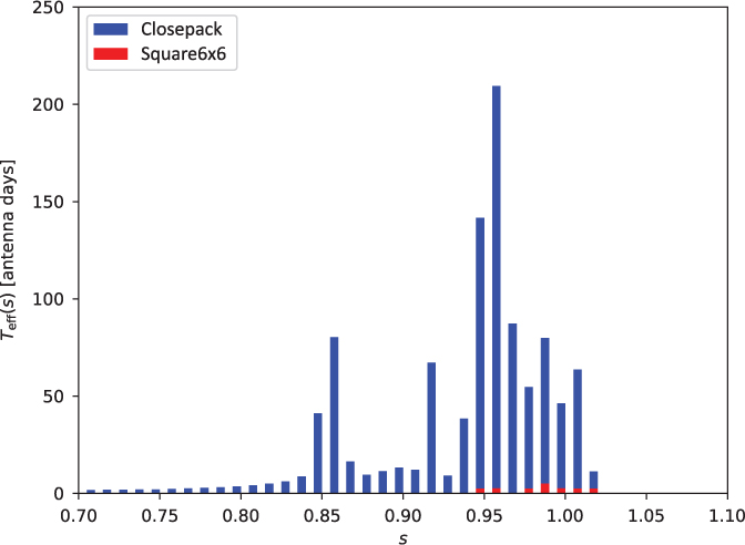
To calculate the time-integrated sensitivity, T _eff(s), the s_i,k are binned with weights equal to the total time-frame of recorded data for each antenna. Due to data losses during commissioning, the recorded data time was found to be 1274.6 antenna days as compared with the nominal time of 1 326 antenna days quoted in Shannon et al. (Reference Shannon2018). A further efficiency factor of 87% was also applied to the observing time, as found in Section 3.2. The total effective observation time, adjusted for efficiency losses, was T _eff = 1108.9 antenna days.

Figure 9 shows T _eff(s). Each ‘spike’ corresponds to an antenna’s base sensitivity, with low-sensitivity tails due to the effects of power noise, which were only significant during closepack36 observations. Most antennas, most of the time, suffered negligible noise effects, and hence their total observation time (antenna days) falls within a single bin.

4.1. Measurements of the beam power pattern

The measurement of each beam power pattern proceeds through the following steps.

1. 1. For each channel, interpolate the real and imaginary components of XX and YY correlation products [Re(C_XX ), Im(C_XX ), Re(C_YY ), Im(C_YY )] from the coarse (15 × 15) measurement grid onto a finer 141 × 141 grid. The SciPy v1.0.0 scipy.interpolate.rectbivariatespline routine in Python 2.7.14 was used with fifth-order splines (Jones et al. Reference Jones2001); the difference with third-order splines in both computational time and final result was negligible.

2. 2. Sum the resulting values to produce a total intensity beam power pattern for each channel, i.e. I = Re²(C_XX ) + Im²(C_XX ) + Re²(C_YY ) + Im²(C_YY ). Note that since one correlating X or Y factor comes from the reference antenna, the correlation powers must be squared to retrieve the beam power pattern of the measurement antenna.

3. 3. Sum I over all channels and calculate a first estimate of the beam centre using the peak value of I.

4. 4. Scale each channel beam about this centre by its frequency in gigahertz, to produce maps in units of degrees gigahertz. Calculate a new average beam over all channels.

5. 5. Correlate each channel beam with the mean beam, and remove those with significantly different shapes.

6. 6. Recalculate a new beam centre and shape using the channels passing the above cuts.

Figure 10.

Example of the beamshape analysis, for antenna 02, beam 00, in closepack36 configuration. Upper left: raw measurements of total power I, averaged over all channels, with blue and red dots showing the expected and first-guess beam centres, respectively. Note the clear presence of RFI near (2.5°, 2.5°). Upper right: interpolated values of I prior to cleaning (‘worst case’ beam). Lower left: cleaned beamshape (‘best case’). Lower right: total closepack36 beamshape in the ‘best case’ scenario, zoomed for clarity. Points indicate the expected beam centres, with circles drawn at the half-power points from an Airy beamshape at 1.296 GHz. The normalisations are (1) each individual channel has its peak power set to unity prior to averaging; (2),(3) the peak value is set to unity, giving a relative beam power pattern; (4) beam 20 is set to unity, and all other peak beam values are set according to the values of b_i found from the pulsar calibration procedure (Section 3). Note that the holography data (top, and lower left, panels) measures the beam position reflected through the origin, which has been corrected-for in the lower right panel.

An example of this procedure is given in Figure 10. Panel 1 shows the raw measurements in |C_XX |² + |C_YY |² read in at step 1, averaged over all channels; panel 2 shows the interpolated values of I calculated at step 3 prior to cleaning; and panel 3 shows the cleaned beams at step 6. The fidelity of each beam can be gauged by the minimum calculated intensity—typically −40 dB after step 5—since any effects such as RFI, mis-formed beams, or deviations from the simple width ∝ 1/f scaling assumed in Step 4 will act to smear the beamshape over the minimum. The greatest limit to beam fidelity is the use of I: repeating the procedure for XX and YY individually resolves much finer structure, but this is not the mode used by CRAFT.

The lower right panel of Figure 10 compares the measured to expected beamshape. As discussed in Section 3, beam 35 is not plotted, since its CRAFT data stream was corrupted. Almost all beams are correctly pointed. Outer beams have their peak sensitivity systematically shifted towards centre (consistent with comatic aberration), while for this particular beamset, beam 26 has a notable azimuthal offset.

Since the beam patterns of each footprint are measured only once with a holographic scan, it is ambiguous whether or not any irregularities present are due to mis-formed beams, or peculiarities at the time of observation. In theory, it should be possible to differentiate by modelling the total received power in the scan, where RFI present during the scan will show up as excess power, while mis-formed beams will not. However, the RMS power in each frequency channel is not well constrained, and the integrated values of XX or YY across the grid—even for ‘good’ channels—fluctuate significantly about the general trend set by the spectrum of Virgo A, making a definition of ‘excess’ power difficult.

The effect of this ambiguity can be calculated by using both cleaned (step 6) and uncleaned (step 3) beams. These correspond to ‘best’ and ‘worst’ cases, respectively, where all irregularities are particular to the holographic scan only, and where they are intrinsic to the beamforming and thus present in CRAFT data.

Figure 11.

Solid angle Ω viewed at a given beam sensitivity, B, for closepack36 (left) and square6×6 (right) configurations. The black lines show Ω for 35 (unphysically) independent Airy beams; green shows Airy beams placed at the locations of each ASKAP beam; purple gives the result when these Airy beams are re-normalised to the beam sensitivities found in Section 3.4.1; and red and blue show the values of Ω derived from the procedure of Section 4.1 in both best (red) and worst (blue) case scenarios. The ‘bumps’ in the Airy beam patterns (e.g. those in the black line near B = 0.4) are due to the grid in solid angle used for integrating Ω(B) as per equation (9), which is identical to that of the ASKAP beam measurements.

A further ambiguity is that the holographic scan region extends only 4.2° in radius, and the beam pattern is typically rotated 45° to the scan grid, meaning that the sidelobes of corner beams are not measured. This is dealt with here by considering two cases: setting all sidelobes in the unmeasured region to zero, and by estimating the beamshape in the unmeasured region to be equal to the measured beamshape reflected through the beam centre. The former case clearly underestimates the power in the sidelobes, while the latter over-estimates it, since the outer beams tend to be more sensitive in the direction of the boresight.

The total normalisation for each beam is determined using the pulsar calibration observations (see Section 3), with outer beams being in general less sensitive than inner beams. As beam 35 is not working, its sensitivity is set to 0, effectively limiting the CRAFT search to 35 beams.

Since the candidate search does not combine information from neighbouring beams, the effective sensitivity of CRAFT FRB searches corresponds to the envelope of all remaining 35 beams. This is calculated for each of the four cases described above. Since sidelobe estimation produces artefacts similar to those in the worst-case scenario, from hereon ‘sidelobes zero’ is synonymous with the ‘best’ case, and ‘estimated sidelobes’ with the ‘worst’ case. An examples of the best- and worst-case beams are given in Figure 10 (lower left and upper right, respectively).

4.1.1. Effects on CRAFT sensitivity

The effects of beamshape on sensitivity to FRBs can be characterised by the solid angle of the sky, Ω, viewed with any given sensitivity, B, to create a histogram Ω(B). This can be thought of as inverting the beamshape B(Ω), although mathematically it is more precisely:

(9) \begin{align}\Omega(B) {\rm d}B = \int \, d \Omega \left\{ \begin{array}{ll}0 & B(\Omega) \lt B, B(\Omega) \ge B+{\rm d}B \\1 & B \le B(\Omega) \lt B+{\rm d}B\end{array} \right.\end{align}

Observe that characterising a beam by a single value of sensitivity, B _eff, and solid angle, Ω_eff, is equivalent to a ‘top-hat’ beamshape with equal sensitivity of B _eff over a solid angle of Ω_eff, and zero otherwise. For such a beam, Ω(B) is

(10) \begin{align}\Omega(B) = \Omega_{\rm eff} \delta(B-B_{\rm eff}) + (4 \pi-\Omega_{\rm eff}) \delta(B)\end{align}

where δ is a Dirac delta function. In general, beams will always view much more of the sky at low sensitivities than high. Both sidelobes, and regions of low primary beam sensitivity, will show up similarly, as large values of Ω(B) for low B.

Figure 11 plots Ω(B) for several cases. The black line shows a simple Airy disc calculated at the mean frequency of 1.296 GHz for a 12-m ASKAP antenna, and multiplied by 35 for comparative purposes. The line increases from right to left, since more of the sky is always viewed at lower sensitivity than high. The same grid is used for calculations as for the beamshapes, which causes both numerical fluctuations, and the value of Ω(B) at 1 to be greater than zero (in the analytic case, an infinitesimal amount of the sky is viewed at peak sensitivity).

The green line shows the effect of overlapping beams, by placing each Airy beam at the true pointing positions of each beam for that footprint. The green and black lines are identical up to the point where the beams begin to overlap, below which the solid angle covered by the beams begins to overlap, and the total solid angle scales less than linearly with the number of beams.

The purple line (‘Corrected Airy beams’) includes the effect of outer beams having reduced sensitivity; the intercept at B = 1 is much lower, since only a few beams have maximum sensitivity; and the point of overlap is also at lower sensitivity.

Upper and lower bounds on CRAFT sensitivity are shown in red (best case, no sidelobe extrapolation) and blue (worst case, with sidelobe extrapolation). These are calculated by averaging over all antennas in the holography observations—error bars are the resulting error in the mean, calculated individually for each bin. Differences between antennas dominate the uncertainty in the region of peak sensitivity (B > 0.5), while systematic effects dominate at low sensitivities (B < 0.4). The effect of using a closely packed PAF beam footprint is evident in the peakedness of Ω(B) above B = 0.6, which is caused by beams obscuring the low-sensitivity regions of neighbouring beams.

Due to holography scans requiring the ASKAP correlator, and CRAFT observations mostly using commissioning antennas which, by definition, are not connected to the correlator, there is no direct way to estimate the beam pattern for all used antennas. Holographic scans are also not performed for every beamforming solution, so that this data set will only be statistically correlated with those used for CRAFT observations. The underlying algorithm for forming PAF beams did remain the same over the course of CRAFT observations. The mean beam- and antenna-dependent factors calculated in Section 3 are thus assumed to average over these time-dependent factors.

Figure 12.

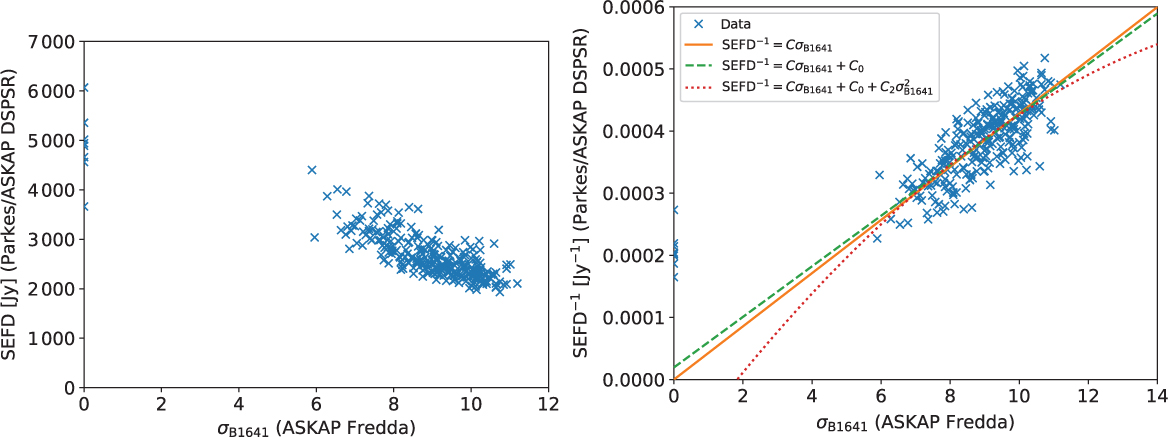
Left: measured sensitivity of ASKAP CRAFT observations, showing system equivalent flux density (SEFD) derived through Parkes–ASKAP observations plotted as a function of CRAFT FREDDA mean pulse height [equation (1)] for each antenna–beam. Right: fits of inverse SEFD as a function of mean pulse height, for different functional forms. The data at σ_B1641 = 0 are from beam 35 and have been excluded from the fit.

5.1. Absolute normalisation

All the above calculations have been of relative sensitivity, specifically by setting that of antenna 8 beam 20 to unity. In order to convert this to an absolute sensitivity, simultaneous observations of B1641 with Parkes (proposal P737) and ASKAP were used to check the absolute sensitivity scale. The observations used the central beam of the Multibeam receiver, with a bandwidth of 256 MHz, centred at 1367.5 MHz. DSPSR (van Straten & Bailes Reference van Straten and Bailes2011) was used to calculate the mean pulse profiles using a total integration time of T _int = 180 s of Parkes and ASKAP data in an offline analysis.

The flux density scale on Parkes was first calibrated using Hydra A, assuming an emission of 43.1 Jy at 1 400 MHz and a spectral index of 0.91 (Scheuer & Williams Reference Scheuer and Williams1968). The mean flux density at pulse peak, $S_{\rm peak}^{\rm B1641}$ , from B1641 was found to be 15.2 ± 0.1 Jy. This allowed the RMS sensitivity of ASKAP, S _rms, to be calculated using the numerical profile values at the peak and off-pulse, $S_{\rm peak}^{\rm num}$ and $S_{\rm off}^{\rm num}$ , giving:

(11) \begin{align}S_{\rm rms} = S_{\rm peak}^{\rm B1641} \frac{S_{\rm off}^{\rm num}}{S_{\rm peak}^{\rm num}}.\end{align}

Inverting the radiometer equation for the observation bandwidth Δv and integration time in each profile bin, T _int/N _bin, the SEFD for CRAFT (total intensity) data can be calculated as follows:

(12) \begin{align}{\rm SEFD} = S_{\rm rms} \sqrt{2 \Delta \nu \, T_{\rm obs}}. \end{align}

The values of the SEFD calculated from equation (12) for each antenna/beam are shown in Figure 12(left), plotted against the fitted mean sensitivity output by FREDDA from ASKAP observations [equation (1)]. The lowest SEFDs (obtained for the central beams) are approximately equal to both preliminary SEFD measurements for ASKAP MkII PAFs of 2000 Jy (Chippendale et al. Reference Chippendale2015) and optimal values of MkI PAFs (McConnell et al. Reference McConnell2016). Beam 35, which detected no pulses when passed through FREDDA (hence σ_B1641 = 0), was found to have a high, but not infinite, SEFD ranging from 3 700–6 100 Jy when analysed with DSPSR.

The SEFD of the data is expected to be inversely proportional to the sensitivity of FREDDA, i.e.

(13) \begin{align}{\rm SEFD}^{-1} = C \sigma_{\rm B1641} \end{align}

for some constant C. This fit is shown in Figure 12(right), where beam 35 data have been excluded. Non-linear effects were tested-for by also fitting first- and second-order polynomials to this range. These did not significantly improve the fits, and, in particular, the concave shape of the second-order fit showed no evidence for an underestimation of the true SEFD when σ_B1641 obtained from FREDDA is low (which would have explained the lack of detections in beam 35).

The cause of the variation in SEFD for a given σ_B1641 is unknown. However, the absolute calibration was performed at a time of high power noise, and it is entirely possible that this induced different responses from DSPSR and FREDDA. A systematic evaluation of pulse search software on common data would contribute greatly to our understanding of this difference.

The constant of proportionality C thus found is (4.28 ± 0.02) × 10⁻⁵ Jy⁻¹, i.e. $\mbox{SEFD}=2.34 \times 10^4 \sigma_{\rm B1641}^{-1}$ . Given the value of 12.44 ± 0.05 fitted for P _B1641 (the mean value of σ_B1641; see Section 3.4.1), this means that the normalised SEFD S ₀ in Section 3 at beam sensitivity B = 1 used in Section 4 corresponds to an SEFD of 1 878 ± 12 Jy. The antenna-averaged value is 1 942 ± 12 Jy, which agrees well with the nominal value of 2 000 Jy. It should be noted however that the uncertainty reflects only the random uncertainty of the fitted means—the variation about the means present in Figure 12 remains an unexplained systematic effect.

5.2. Detection threshold

The nominal fluence detection threshold F ₀ to a perfectly de-dispersed FRB with duration contained entirely within the integration time t _int = 1.2656 ms is

(14) \begin{align}F_{0} = \frac{\sigma_{\rm th} \mbox{SEFD}}{\sqrt{2 t_{\rm int} \Delta \nu}}. \end{align}

For the CRAFT bandwidth of Δv = 336 MHz, time resolution of t _int 1.2656 ms, SEFD of 1 890 ± 13 Jy, and detection threshold σ_th = 9.5, this corresponds to F ₀ = 24.6 ± 0.2 Jy ms (25.5 ± 0.2 Jy ms antenna-average, i.e. consistent with the nominal value of 26 quoted in Shannon et al. Reference Shannon2018). The actual threshold will differ from this value for any real FRB and search method, as discussed in Section 6.

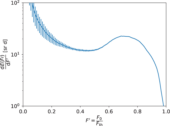
The total CRAFT exposure E as a function of fluence threshold F _th can be accounted for by integrating the beam-dependence Ω(B) from equation (9) (displayed in Figure 11) with the time- and antenna-dependence T(S′) given in Figure 9, and applying the normalisation F ₀ = 24.8 ± 0.2 Jy ms. Summing this over both closepack36 ‘cp’ and square6×6 ‘sqr’ periods produces the survey exposure E as a function of fluence threshold F _th:

(15) \begin{align}E(F_{\rm th}) &= \sum_{i={\rm cp,sqr}} \int {\rm d}B \, \Omega_{i}(B) \, T_i(S^{\prime}) \nonumber \\S^{\prime} &= B \frac{F_0}{F_{\rm th}}.\end{align}

This is given in Figure 13, in terms of $\frac{{\rm d}E}{{\rm d}F}$ , and relative fluence sensitivity $F^\prime = \frac{F_0}{F_{\rm th}}$ . Note that the contribution from the square 6×6 configuration is small, since the majority of observations were made in closepack36 configuration—Figure 11 gives a much better comparison of the relative sensitivities of the two configurations.

Figure 13.

Exposure E of the CRAFT high Galactic latitude survey in terms of relative sensitivity F′ = F ₀/F _th, defined such that the integral over F comes to the corrected observation time T′ = 1 208 d. The mean value is calculated using the average of best case and worst case beam estimated (Figure 10), while errors are calculated from the systematic difference between the mean and these cases, added in quadrature to the random uncertainty in the mean.

5.3. Effective survey parameters

For an FRB population with a power-law spectrum of fluences, such that the detection rate R has the form:

(16) \begin{align}R(F_{\rm th},\alpha) = k \left(\frac{F_{\rm th}}{F_0}\right)^{\alpha}\!\left[{\rm sky}^{-1} {\rm d^{-1}}\right] \end{align}

for some constant k, fluence threshold F _th relative to some value F ₀, and spectral index α, the number N of detected FRBs in a survey will be

(17) \begin{align}N(\alpha) = \int {\rm d}F_{\rm th} \, E(F_{\rm th}) \, R(F_{\rm th},\alpha). \end{align}

In cases where the only modelled sensitivity dependence is the beamshape, equation (17) reduces to

(18) \begin{align}N(\alpha) & = T_{\rm eff} \int {\rm d}F_{\rm th} \, \Omega\!\left(B=\frac{F_0}{F_{\rm th}}\right)\! R(F_{\rm th},\alpha)\end{align}

(19) \begin{align} = T_{\rm eff} \int {\rm d}\Omega \, B(\Omega) \, R(F_{\rm th}=F_0/B,\alpha)\end{align}

for effective observation time T _eff, and B and Ω(B) defined according to equation (9).

Comparisons between different FRB surveys however tend to characterise each in terms of a single fluence threshold F _eff(α) and exposure E _eff(α), which are both functions of α as discussed by Macquart and Ekers (Reference Macquart and Ekers2018). Defining these to keep N constant:

(20) \begin{align}N(\alpha) = E_{\rm eff}(\alpha) \, R(F_{\rm eff},\alpha) \end{align}

and separating exposure into effective observation time T _eff (here antenna days) and solid angle Ω_eff(α):

(21) \begin{align}E_{\rm eff}(\alpha) = T_{\rm eff} \, \Omega_{\rm eff}(\alpha)\end{align}

produces an ambiguity between effective sensitive area Ω_eff and effective threshold F _eff.

There are three natural constraints to remove this ambiguity. The simplest is to set the threshold F _eff equal to the nominal threshold F ₀ at beam centre, and modify the exposure accordingly, i.e.

(22) \begin{align}\Omega_{\rm eff}(\alpha) & = T_{\rm eff}^{-1}\int {\rm d}F_{\rm th} \, E(F_{\rm th}) \frac{R(F_{\rm th},\alpha)}{R(F_0,\alpha)} \nonumber \\& = T_{\rm eff}^{-1} \int {\rm d}F_{\rm th} \, E(F_{\rm th}) \left( \frac{F_{\rm th}}{F_0} \right)^{\alpha}\!. \end{align}

This figure can be misleading, however, because F ₀ is not characteristic of the detected FRB fluences.

This effect can be accounted for by defining F _eff(α) as being equal to the mean threshold $\bar{F}_{\rm th}(\alpha)$ :

(23) \begin{equation}\bar{F}_{\rm th}(\alpha) = \frac{1}{N(\alpha)} \int {\rm d}F_{\rm th} \, F_{\rm th} \, E(F_{\rm th}) \, R(F_{\rm th},\alpha) \end{equation}

or to the mean true fluence $\bar{F}_{\rm true}$ of detected FRBs:

(24) \begin{align}\bar{F}_{\rm true}(\alpha) & = \frac{1}{N(\alpha)} \int {\rm d}F_{\rm th} E(F_{\rm th})\int_{F_{\rm th}}^{\inf} dF^\prime F^\prime \frac{{\rm d} R(F^\prime,\alpha)}{{\rm d}F^\prime} \nonumber \\& = \frac{1}{N(\alpha)} \int {\rm d}F_{\rm th} E(F_{\rm th}) \frac{\alpha}{\alpha+1} F_{\rm th} R(F^\prime,\alpha) \nonumber \\& = \frac{\alpha}{\alpha+1} \bar{F}_{\rm th}(\alpha).\end{align}

The difference between these two measures only becomes important when models deviating from a pure power law are being fitted, in which case experimental sensitivity should not be reduced to a single effective threshold.

Here, we choose $F_{\rm eff} \equiv \bar{F}_{\rm th}$ . This then defines Ω_eff(α) through equation (20), or by replacing F ₀ by $\bar{F}_{\rm th}$ in equation (22).

It is important to note that equation (23) becomes ill-defined as α approaches unity, which can be seen through the dependence of the integrand on α:

(25) \begin{equation}\bar{F}_{\rm th}(\alpha) \propto \int {\rm d}F_{\rm th} \, F_{\rm th}^{\alpha+1} \, E(F_{\rm th}). \end{equation}

Even as F _th approaches zero, its contribution to the integrand remains constant when α = −1, and the integral in equation (25) evaluates to 4πT _eff (i.e. the total exposure at all sensitivities). This can be understood as a very small number of expected detections at very low sensitivity (e.g. in a beam’s far sidelobes) contributing correspondingly large values of true fluence threshold F _th. As α approaches −1, the result for $\bar{F}_{\rm th}$ becomes highly dependent on numerical details, e.g. histogram bin width in the exposure function E, and the distance out to which Ω(B) is evaluated. This is not the case for the choice of $F_{\rm eff} \equiv F_0$ , where Ω_eff [equation (22)] remains defined for α < 0. However, this should be viewed as an advantage, serving as a reminder that as α approaches −1, the true fluences of detected FRBs become poorly correlated with any choice of effective threshold F _eff, so that the ease of calculation for the choice $F_{\rm eff} \equiv F_0$ merely provides a false sense of security.

Figure 14.

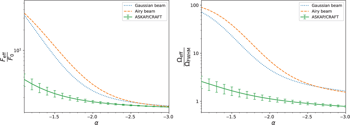
Effective observation parameters relative to their nominal values: effective fluence threshold F _eff/F ₀ (left) and effective survey area Ω_eff/Ω_FWHM (right). CRAFT GL50 results are calculated from the mean of the best- and worst-case scenarios of Ω(B), with errors showing the systematic range corresponding to using each scenario. This is compared to results from single Airy and Gaussian beams. F ₀ is relative to peak central beam sensitivity, while Ω_FWHM is calculated as the beam full width half maximum for an Airy disc at central frequency.

5.3.1. Effective survey parameters: results

For the CRAFT GL50 survey, both F _eff(α) and Ω_eff(α), calculated as per equations (23) and (20). respectively, are shown in Figure 14. For comparison, results using single Airy and Gaussian beams are also shown.

In interpreting the result, note that F _eff will always be greater than the nominal sensitivity F ₀ at beam centre. As α tends to −1, there are more FRBs with large amplitude. The effects of sidelobes become increasingly important, and Ω_eff will be larger than quoted values (typically the area at full width half maximum). Conversely, as α tends to negative infinity, F _eff will tend to F ₀, and Ω_eff will tend to zero. In the case that α > −1, observations will be so biased towards high-luminosity FRBs detected far from beam centre that any definition of F _eff will be physically meaningless. However, observations do not appear to be in this regime, given the current best fit to ASKAP/CRAFT data of α = −2.2, and α = −1.2 for Parkes (James et al. Reference James, Ekers, Macquart, Bannister and Shannon2018).

The effect of the overlapping beams used in CRAFT surveys is immediately apparent in Figure 14. This flattens the dependence of F _eff and Ω_eff on α, whereas for Gaussian or Airy beams, these parameters vary by an order of magnitude between α = −1 and α = −3. The errors due to the uncertainty in the shape of the sidelobes of outer ASKAP beams become more important at low values of α.

As discussed in the previous section, the calculation is expected to become numerically unstable near α = −1. However, the measurement of the beam over a finite patch of sky effectively cuts off the integration in equation (23), achieving numerical stability at the cost of physical accuracy. To estimate the magnitude of this effect, we calculated F _eff(α) for the closepack36 configuration using Gaussian beamshapes, both with and without limiting the integral to the 8.4° × 8.4° region of the holography scans. The resulting error in F _eff was less than that due to the beamshape for α ≤ −1.1. The calculations for Gaussian and Airy beams are exact.

The values from Figure 14 are compiled in Table 2. The relative increases in F _eff and Ω_eff compared to nominal values are also given, which is particularly useful for scaling results from other experiments.

Table 2.

Tabularised effective CRAFT survey parameters as a function of FRB source counts index α. Parameters are the effective fluence threshold F _eff, nominal threshold at beam centre F ₀, effective solid angle Ω_eff, and nominal solid angle at full width half maximum Ω_FWHM. The effective rate R is also calculated, corresponding to 19 FRBs over T _eff = 1108.9 antenna days. Mean values and errors are systematic (‘sys’) and correspond to the means and errors from the exposure E in Figure 13. The exception is the statistical error (‘stat’) in the rate R corresponding to Poisson fluctuations in the number of observed FRBs. These are shown as the second, symmetric component of the error in R.

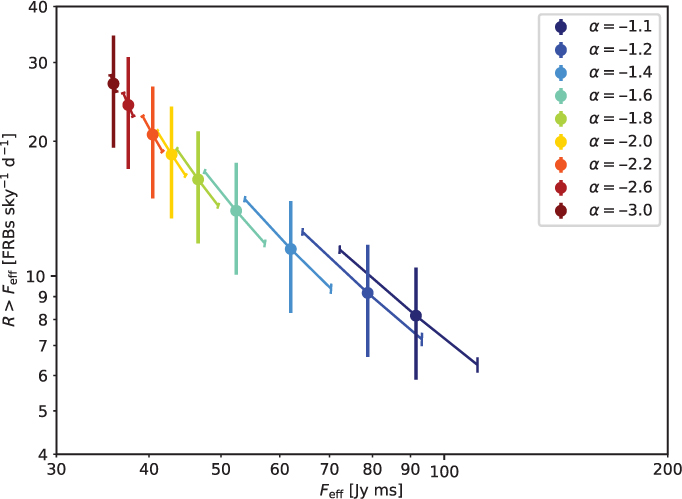
Using the 19 FRBs detected above threshold (FRB 171216 was detected only using a combination of beams in a non-standard analysis, and falls below the threshold calculated here), Figure 15 shows the measured all-sky (4π sr) rates as a function of both α and F _eff. For the range of α from −1.5 to −2.7 reported by James et al. (Reference James, Ekers, Macquart, Bannister and Shannon2018) (68% confidence), the rate varies between 12.7 and 24.9 FRBs sky⁻¹ d⁻¹, above thresholds of 57 and 37 Jy ms, respectively. The error resulting from uncertainties in F _eff and Ω_eff is approximately equal in impact to an uncertainty in α of ±0.2, and is the dominant source of error for α > −1.4.