





1. Introduction
In their article [Reference Becker and Döring9], Becker and Döring provided one of the earliest descriptions of particle growth in the theory of nucleation from supersaturated vapour, which subsequently gave the name to the model. This model describes the growth and decay of clusters, consisting of identical monomers, only by the addition and removal of monomers. The modern formulation of the equations seems to go back to Burton [Reference Burton and Bruce14] to study condensations phenomena at different pressures and was popularised among mathematicians by Penrose and Lebowitz [Reference Penrose and Lebowitz43]. Since then, the model has been applied in a variety of fields, including but not limited to physics, chemistry and biology. Initial mathematical results were proved by Ball, Carr and Penrose [Reference Ball and Carr5, Reference Ball, Carr and Penrose7], then the mathematical aspect of these equations has been studied in detail. Well-posedness and many aspects of the long-time behaviour of solutions are understood [Reference Cãnizo, Einav and Lods16, Reference Cañizo and Lods15, Reference Jabin and Niethammer32] and many other works, as well as the emergence of phase transition [Reference Penrose42]. However, there are still open questions, see, e.g. [Reference Hingant and Yvinec31] and [Reference Wattis46].
We also point out the fact that the Becker–Döring equations are a specific case of general discrete coagulation-fragmentation equations. Therefore, classical results, mainly on the well-posedness, can be applied. First, mathematical results were proved by Ball and Carr [Reference Ball and Carr6], Carr [Reference Carr17], Carr and da Costa [Reference Carr and da Costa18], and da Costa [Reference da Costa19] on the well-posedness and the asymptotic behaviour of solutions. Another proof of existence was found by Laurençot [Reference Laurençot and Mischler35] extending existence result of Carr and da Costa [Reference Carr and da Costa18].
In this work, we study a variant of Becker–Döring equations. We have in mind specific applications to biology with polymerisation of biomolecules such as fibrin clots formation. It is thus natural to consider open systems in which monomers arise from a reaction cascades (e.g. fibrinogen conversion to fibrin protein), and a fragmentation process undergoes an irreversible process such as fibrin digestion by plasmin [Reference Longstaff and Kolev39]. In our version of Becker–Döring equations, we consider a model where injection of monomers is constant, which may represent synthesis of fibrin monomer, and the detached monomer from fragmentation is not able to go through the coagulation process again. The reactions taking place are given by
 \begin{equation*}\left \{ \begin{aligned} (1) + (i) &\xrightarrow []{a_{i}} (i+1), \,i\geq 1, \\ (i) &\xrightarrow []{b_i} (i-1), \,i\geq 3, \\ (2) &\xrightarrow []{b_2} \emptyset , \\ \emptyset &\xrightarrow []{\lambda } (1), \end{aligned} \right . \end{equation*}
where $(i)$
represents the concentration of clusters of size
$(i)$
represents the concentration of clusters of size $i$
. The non-negative numbers
$i$
. The non-negative numbers $a_i$
and
$a_i$
and $b_i$
denote, respectively, the coagulation and fragmentation coefficients. It is important to note that the
$b_i$
denote, respectively, the coagulation and fragmentation coefficients. It is important to note that the $(2) \xrightarrow []{b_2} \emptyset$
reaction is the result of a specific choice that was made, namely that a 2-polymer should disappear and not form a single monomer. The degradation of the 2-polymer is presumed to occur in a manner that both monomers are degraded. We believe that with slight adaptations, our results hold with considering the reaction
$(2) \xrightarrow []{b_2} \emptyset$
reaction is the result of a specific choice that was made, namely that a 2-polymer should disappear and not form a single monomer. The degradation of the 2-polymer is presumed to occur in a manner that both monomers are degraded. We believe that with slight adaptations, our results hold with considering the reaction $(2) \xrightarrow []{b_2} (1)$
.
$(2) \xrightarrow []{b_2} (1)$
.
The infinite system of ordinary differential equations associates to the reaction scheme is
 \begin{equation} \left \{ \begin{aligned} \frac {d}{dt}C_1(t) &= \lambda - \sum _{j=1}^{+\infty }a_{j}C_1(t)C_j(t) - a_1C_1(t)^2, & \\ \frac {d}{dt}C_i(t) &= J_{i-1}(t) - J_i(t), & i\geq 2, \end{aligned} \right . \end{equation}
where, for all $i\geq 1$
,
$i\geq 1$
,
 \begin{equation} J_i(t) = a_iC_1(t)C_i(t) - b_{i+1}C_{i+1}(t). \end{equation}
The unknowns are the functions $C = (C_i(t))_{i\geq 1}$
that depend on time
$C = (C_i(t))_{i\geq 1}$
that depend on time $t\geq 0$
and where, for each
$t\geq 0$
and where, for each $i\in \mathbb{N}^\ast$
,
$i\in \mathbb{N}^\ast$
, $C_i(t)$
denotes the concentration of
$C_i(t)$
denotes the concentration of $i$
-particles clusters per unit of volume at time
$i$
-particles clusters per unit of volume at time $t$
. The quantity
$t$
. The quantity $J_i$
does not represent the rate of change of a reversible reaction as in the Becker–Döring equations, but for convenience, we keep this notation.
$J_i$
does not represent the rate of change of a reversible reaction as in the Becker–Döring equations, but for convenience, we keep this notation.
Some work already exists on models close to Becker–Döring and close to ours. The first modification was to add monomers injection; it appears in submonolayer epitaxial growth [Reference Amar and Family2, Reference Bales and Chrzan4], in nucleation theory for thin film growth [Reference Ratsch and Venables44]. The first mathematical work was done by Blackman and Marshall [Reference Blackman and Marshall10], they discussed scaling behaviour and growth exponent for a constant rate source; then by Wattis [Reference Wattis45] where he studied self-similar behaviour of solutions for a time-dependent monomer input and size-independent rate coefficients. He has already shown that with a slight modification, the long-time behaviour of solutions may become complex and depend strongly on the production rate. We also mention the works of da Costa et al. [Reference da Costa, Pinto and Sasportes21, Reference da Costa, Pinto and Sasportes22] and [Reference da Costa, van Roessel and Wattis23], which, with constant rate coefficients, complement some of the formal results in [Reference Blackman and Marshall10] and [Reference Wattis45]. Recently, Niethammer et al. [Reference Niethammer, Pego, Schlichting and Velázquez41] introduced a depletion term representing clusters removal. As our model, the chemical reaction network is open, it then becomes unclear whether long-time convergence towards steady-state holds. In their case, they provide evidence for the persistence of oscillations in time. We also mention the work of Bolton and Wattis [Reference Bolton and Wattis13], in which they considered a model with injection, competition and inhibition.
There exist other modifications of the Becker–Döring equations but differs to ours, for example, the work of Doumic et al. [Reference Doumic, Fellner, Mezache and Rezaei24] introduces a bi-monomeric model explaining oscillations. We also mention the work of Wattis [Reference Wattis47] in which the fragmentation rates depend on the total number of clusters present in the system and the works of Laurençot and Wrzosek [Reference Laurençot and Wrzosek36] and [Reference Laurençot and Wrzosek37] in which they added space diffusion.
Some literature exists on continuous models with mass loss, more specifically on coagulation and fragmentation equations with discrete and continuous mass loss. The first mathematical work was done by Edwards [Reference Edwards, Cai and Han27], and a more recent work was done by Blair et al. [Reference Blair, Lamb and Stewart11]. A part of the book of Banasiak, Lamb and Laurençot [Reference Banasiak, Lamb and Laurencot8] treats those equations using semigroups techniques. Different authors [Reference Ali, Barik and Giri1] and [Reference Baird and Süli3] considered a hybrid model of fragmentation still with discrete and continuous mass loss.
In this work, we start by proving well-posedness of (1.1). The proof of existence follows that of Laurençot [Reference Laurençot34], which, as for the proof of Ball et al. [Reference Ball and Carr6] and [Reference Ball, Carr and Penrose7], relies on a truncated system and compactness arguments to obtain the limit. Uniqueness is more classical and follows the initial work of Ball and Carr [Reference Ball and Carr6]. As in the Becker–Döring equations, two distinct cases appear; however, here it does not depend on the initial mass, since our system does not preserve it, but instead on the production rate $\lambda$
. There is a threshold
$\lambda$
. There is a threshold $\lambda _s$
, which dictates significant change in the dynamic. In the sub-critical case
$\lambda _s$
, which dictates significant change in the dynamic. In the sub-critical case $\lambda \leq \lambda _s$
, it may occur that
$\lambda \leq \lambda _s$
, it may occur that
-
• either there exists a unique steady state for $b_i \leq ia_i$
,
$b_i \leq ia_i$
, -
• or there exists an infinite number of steady states for
$b_i \gt i^\nu a_i$
with
$\nu \gt 1$
.


We prove that if $\lambda$
is sufficiently small and
$\lambda$
is sufficiently small and $a_i \lt b_i \leq i$
, then the steady state is locally exponentially asymptotically stable. This corresponds to
$a_i \lt b_i \leq i$
, then the steady state is locally exponentially asymptotically stable. This corresponds to $b_i$
strong enough but not too much (moderate); these conditions will be made precise in the Section 2.2.3. In the super-critical case
$b_i$
strong enough but not too much (moderate); these conditions will be made precise in the Section 2.2.3. In the super-critical case $\lambda \gt \lambda _s$
, contrary to the Becker–Döring equations, we do not find a Lyapunov functional; thus, we were not able to prove a result in the super-critical case. The question remains open, but we expect some self-similar behaviour of the solution [Reference Wattis45]. We end this work with a numerical scheme. We develop, on the conservative truncation, a well-balanced and coarse-grained scheme, which consists of sub-sampling the clusters at some given size, preserving the asymptotics. The scheme is based on the flux approximation scheme of Ducan and Soheili [Reference Duncan and Soheili26] and the well-balanced scheme of Goudon and Monasse [Reference Goudon and Monasse29]. This scheme can be used on the classical Becker–Döring equations.
$\lambda \gt \lambda _s$
, contrary to the Becker–Döring equations, we do not find a Lyapunov functional; thus, we were not able to prove a result in the super-critical case. The question remains open, but we expect some self-similar behaviour of the solution [Reference Wattis45]. We end this work with a numerical scheme. We develop, on the conservative truncation, a well-balanced and coarse-grained scheme, which consists of sub-sampling the clusters at some given size, preserving the asymptotics. The scheme is based on the flux approximation scheme of Ducan and Soheili [Reference Duncan and Soheili26] and the well-balanced scheme of Goudon and Monasse [Reference Goudon and Monasse29]. This scheme can be used on the classical Becker–Döring equations.
2. Main results
In this section, we introduce some notations, hypotheses and state the main results. Details and proofs are presented in their respected section. Before starting our existence and uniqueness result, we provide the definition of a solution to (1.1).
Definition 2.1.
Let $T\in (0,+\infty ]$
. A solution
$T\in (0,+\infty ]$
. A solution $C = (C_i)_{i\geq 1}$
of (
1.1
) on
$C = (C_i)_{i\geq 1}$
of (
1.1
) on $[0,T)$
is a sequence of non-negative functions satisfying the following conditions for all
$[0,T)$
is a sequence of non-negative functions satisfying the following conditions for all $i\geq 1$
,
$i\geq 1$
, $t\in [0,T)$
,
$t\in [0,T)$
,
-
(i)
$C_i \in \mathcal{C}^0([0,t))$
,
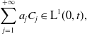
$\,\displaystyle \sum _{j=1}^{+\infty } a_{j}C_j \in \mathrm{L}^1(0,t),$
-
(ii) and there holds
\begin{equation*} \left \{ \begin{aligned} C_1(t) &= C_1(0) + \lambda t - \int _0^t C_1(s)\sum _{j=1}^{+\infty }a_{j}C_j(s) - a_1C_1(s)^2 ds , & i=1 \\ C_i(t) &= C_i(0) + \int _0^t \left [ J_{i-1}(s) - J_i(s)\right ]ds, & i\geq 2. \end{aligned} \right . \end{equation*}


We start by stating the weak form of (1.1), which is very useful to compute moments or to find some uniform bounds.
Proposition 2.2.
Let $C$
be a solution of (
1.1
). For all compactly supported sequences
$C$
be a solution of (
1.1
). For all compactly supported sequences $(\varphi _i)_{i\geq 1}$
, we have
$(\varphi _i)_{i\geq 1}$
, we have
 \begin{equation} \frac {d}{dt}\sum _{i=1}^{+\infty } \varphi _iC_i = \lambda \varphi _1 - \varphi _2b_2C_2 + \sum _{i=1}^{+\infty } \left [\varphi _{i+1}-\varphi _i-\varphi _1\right ]a_iC_1C_i + \sum _{i=3}^{+\infty } \left [\varphi _{i-1}-\varphi _i\right ]b_iC_i. \end{equation}
We can write it under another form as follows:
 \begin{equation} \frac {d}{dt}\sum _{i=1}^{+\infty } \varphi _iC_i = \varphi _1\left (\lambda -b_2C_2 - \sum _{i=2}^{+\infty } b_iC_i\right ) + \sum _{i=1}^{+\infty } \left [\varphi _{i+1}-\varphi _i-\varphi _1\right ]\left (a_iC_1C_1-b_{i+1}C_{i+1}\right )\!. \end{equation}
We define the following Banach spaces in which solutions will lie. Let $\alpha \geq 0$
, we define the following subspaces of
$\alpha \geq 0$
, we define the following subspaces of $\ell ^1(\mathbb{R})$
,
$\ell ^1(\mathbb{R})$
,
 \begin{equation*} X_\alpha \,:\!= \left \{ x = (x_k)_{k\geq 1} \in \mathbb{R}^{\mathbb{N}} \;:\; \|x\|_{X_\alpha } \,:\!= \sum _{k=1}^{+\infty } k^\alpha |x_k| \lt +\infty \right \}\!, \end{equation*}
and we denote $X_\alpha ^+$
its positive cone. Some of these spaces have physical meaning, for example, the norm in
$X_\alpha ^+$
its positive cone. Some of these spaces have physical meaning, for example, the norm in $X_0 = \ell ^1$
is proportional to the total number of clusters, or the norm of
$X_0 = \ell ^1$
is proportional to the total number of clusters, or the norm of $X_1$
is proportional to the mass of all the clusters in our system. Some properties of these spaces can be found in the review of da Costa [Reference da Costa20, Section 2.1].
$X_1$
is proportional to the mass of all the clusters in our system. Some properties of these spaces can be found in the review of da Costa [Reference da Costa20, Section 2.1].
2.1. Well-posedness
We state the main results on existence and uniqueness of solutions under some assumptions on the kinetic coefficients, mainly on the coagulation ones, and on the initial data. Let $\alpha \in [0,1]$
.
$\alpha \in [0,1]$
.
-
(H1) There exists
$a \geq 0$
such that
$0 \leq a_{i} \leq a i^\alpha$
and
$b_i \geq 0$
for all
$i\geq 1$
.


In the classical proof of existence from Ball, Carr and Penrose [Reference Ball, Carr and Penrose7] or for the general coagulation-fragmentation equations from [Reference Ball and Carr6] or [Reference Laurençot34], the natural space for the existence is $X_1$
since the equations are mass preserving. Here, equations (1.1) do not preserve mass; therefore, we can consider a larger space for the existence, in which mass does not necessarily have meaning or may blow up. We have the following existence results in
$X_1$
since the equations are mass preserving. Here, equations (1.1) do not preserve mass; therefore, we can consider a larger space for the existence, in which mass does not necessarily have meaning or may blow up. We have the following existence results in $X_\alpha$
for
$X_\alpha$
for $\alpha \in [0,1]$
.
$\alpha \in [0,1]$
.
Theorem 2.3 (Existence and moment spreading). Let $C^{init} \in X_\alpha ^+$
. Under the hypothesis (H1), there exists at least one solution
$C^{init} \in X_\alpha ^+$
. Under the hypothesis (H1), there exists at least one solution $C \in \mathcal{C}^0([0,+\infty ),X_\alpha ^+)$
to (
1.1
) with initial data
$C \in \mathcal{C}^0([0,+\infty ),X_\alpha ^+)$
to (
1.1
) with initial data $C(0) = C^{init}$
. Moreover, if there exists
$C(0) = C^{init}$
. Moreover, if there exists $\mu \geq \alpha$
such that
$\mu \geq \alpha$
such that
 \begin{equation*} \sum _{i=1}^{+\infty } i^\mu C_i^{init} \lt +\infty , \end{equation*}
then any solution satisfies for all $T\gt 0$
 \begin{equation*} \sup _{t\in [0,T]}\sum _{i=1}^{+\infty } i^\mu C_i(t) \lt +\infty . \end{equation*}
We actually prove a more general result including more than just power law moments but a wider class, see Section 3. This theorem is inspired by [Reference Laurençot34, Theorem 2.5], and it generalises [Reference Carr and da Costa18, Theorem 3.3], which proves moment spreading in coagulation-fragmentation equations.
Theorem 2.4 (Partial uniqueness). Let $C^{init}\in X_\alpha ^+$
and
$C^{init}\in X_\alpha ^+$
and $T\in (0,+\infty ]$
. Under the hypothesis (H1), there exists at most one solution
$T\in (0,+\infty ]$
. Under the hypothesis (H1), there exists at most one solution $C$
to (
1.1
) on
$C$
to (
1.1
) on $[0,T)$
with initial condition
$[0,T)$
with initial condition $C(0)=C^{init}$
such that
$C(0)=C^{init}$
such that
 \begin{equation} C \in \mathrm{L}^\infty ([0,t],X_\alpha ^+) \text{ and } \sum _{i=1}^{+\infty } i^{2\alpha } C_i \in \mathrm{L}^1(0,t) \text{ for all } t \in (0,T). \end{equation}
Theorem 2.5 (Well-posedness). Let $C^{init}\in X_{2\alpha }^+$
and
$C^{init}\in X_{2\alpha }^+$
and $T\in (0,+\infty ]$
. Under the hypothesis (H1), there exists a unique solution
$T\in (0,+\infty ]$
. Under the hypothesis (H1), there exists a unique solution $C$
to (
1.1
) on
$C$
to (
1.1
) on $[0,T)$
with initial condition
$[0,T)$
with initial condition $C(0)=C^{init}$
. Moreover, this solution satisfies
$C(0)=C^{init}$
. Moreover, this solution satisfies
 \begin{equation*} C \in \mathcal{C}^0([0,t],X_\alpha ^+) \text{ and } \sum _{i=1}^{+\infty } i^{2\alpha } C_i \in \mathrm{L}^1(0,t) \text{ for all } t \in (0,T). \end{equation*}
Theorem2.5 is an immediate consequence of Theorems2.4 and 2.3. The partial uniqueness result Theorem2.4 is inspired by [Reference Ball and Carr6, Theorem 4.2] and [Reference Laurençot34, Proposition5.1] and state uniqueness under moments control. Laurençot and Mischler [Reference Laurençot and Mischler35, Theorem 2.1] gave another proof of uniqueness, on the Becker–Döring equations, without the assumption on moments control, but with an assumption on coefficients $(b_i)_{i\geq 1}$
. Their proof is based on estimates of distribution tails and mass conservation. The proof of Theorem2.4 is given in Section 4.
$(b_i)_{i\geq 1}$
. Their proof is based on estimates of distribution tails and mass conservation. The proof of Theorem2.4 is given in Section 4.
In the remainder, we will always assume that the kinetics coefficients satisfy the condition (H1) for some suitable $\alpha \in [0,1]$
.
$\alpha \in [0,1]$
.
2.2. Long-time behaviour
2.2.1. Uniform-in-time bound
The first uniform-in-time bound is an upper bound on $C_1(t)$
. We obtain directly from the equation on
$C_1(t)$
. We obtain directly from the equation on $C_1$
that for all
$C_1$
that for all $t\in [0,+\infty )$
, we have
$t\in [0,+\infty )$
, we have
 \begin{equation} C_1(t) \leq \kappa (\lambda ,C^{init}) \,:\!= \max \left \{C_1^{init},\sqrt {\frac {\lambda }{2a_1}}\right \}\!. \end{equation}
We prove an upper uniform-in-time bound on exponential moments under strong fragmentation, and this will allow us to prove the local exponential stability of a steady state. The following proposition is inspired by a similar result in [Reference Jabin and Niethammer32, Lemma 3.3].
Proposition 2.6 (Exponential moments uniform-in-time bound). Assume that the kinetics coefficients satisfy the following conditions:
 \begin{equation} \forall i\geq 1, \,a_i \geq \underline {a} \gt 0. \end{equation}
Let $\lambda \geq 0$
and
$\lambda \geq 0$
and $C^{init}$
small enough such that
$C^{init}$
small enough such that
 \begin{equation} \kappa (\lambda ,C^{init}) \lt \inf _{i\geq 1} \frac {b_i}{a_i}, \end{equation}
and there exists $\nu \gt 0$
such that
$\nu \gt 0$
such that
 \begin{equation} \sum _{i=1}^{+\infty } e^{\nu i}C_i^{init} \lt +\infty . \end{equation}
Then, there exists a constant $\Xi _1 \gt 0$
such that for all
$\Xi _1 \gt 0$
such that for all $t\geq 0$
,
$t\geq 0$
,
 \begin{equation} \sum _{i=1}^{+\infty } e^{\nu i}C_i(t) \leq \Xi _1, \end{equation}
where $\Xi _1$
depends only on
$\Xi _1$
depends only on $\lambda$
,
$\lambda$
, $(a_i)_{i\geq 1}$
,
$(a_i)_{i\geq 1}$
, $(b_i)_{i\geq 1}$
,
$(b_i)_{i\geq 1}$
, $\nu$
and initial data.
$\nu$
and initial data.
We also prove, under some hypotheses on the kinetic coefficients, an upper bound on the mass and a lower bound on $C_1$
. Details and proofs are presented in Section 5.1.
$C_1$
. Details and proofs are presented in Section 5.1.
2.2.2. Steady states
We define the detailed balance coefficients $Q_i$
by
$Q_i$
by
 \begin{equation} Q_1 \,:\!= 1,\,\, Q_i \,:\!= \prod \limits _{j=2}^i \frac {a_{j-1}}{b_j}, \text{ pour } i\geq 2. \end{equation}
These coefficients play a significant role in the long-term behaviour of the solutions. It is from these coefficients that two significant quantities are defined. The first quantity is the critical monomer density, denoted $z_s$
, which is defined as the radius of convergence of the power series
$z_s$
, which is defined as the radius of convergence of the power series $\sum a_iQ_iz^i$
. This quantity is also called monomer saturation density, hence the subscript. The second quantity is the critical production threshold, denoted
$\sum a_iQ_iz^i$
. This quantity is also called monomer saturation density, hence the subscript. The second quantity is the critical production threshold, denoted $\lambda _s$
, which is defined as follows:
$\lambda _s$
, which is defined as follows:
 \begin{equation} \lambda _s \,:\!= \sup _{z\leq z_s} \sum _{j=1}^{+\infty } a_jQ_jz^{j+1} + a_1 z^2. \end{equation}
We emphasise that both $z_s$
and
$z_s$
and $\lambda _s$
are completely determined by the coefficients
$\lambda _s$
are completely determined by the coefficients $a_i$
and
$a_i$
and $b_i$
.
$b_i$
.
Remark 2.7.
As the function $z\mapsto a_jQ_jz^{j+1}$
is increasing, the critical production threshold can be rewritten, when the series converges, as follows:
$z\mapsto a_jQ_jz^{j+1}$
is increasing, the critical production threshold can be rewritten, when the series converges, as follows:
 \begin{equation*} \lambda _s = \sum _{j=1}^{+\infty } a_jQ_jz_s^{j+1} + a_1 z_s^2. \end{equation*}
In the following, we add two hypotheses that can be readily verified in the case of constant coefficients, certain power laws or Niethammer’s coefficients [Reference Niethammer40, (1.5) and (1.6)]. These conditions are as follows.
-
(H2) There exists
$\underline {a}\gt 0$
and
$\underline {b}\gt 0$
such that
$\inf \limits _{i\geq 1}a_i=\underline {a}$
and
$\inf \limits _{i\geq 1}b_i=\underline {b}$
, -
(H3) There exists
$l\gt 0$
such that
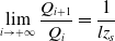
$\lim \limits _{i\to +\infty }\dfrac {Q_{i+1}}{Q_i}=\dfrac {1}{l z_s}$
, -
(H4)
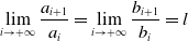
$\lim \limits _{i\to +\infty }\dfrac {a_{i+1}}{a_i} = \lim \limits _{i\to +\infty }\dfrac {b_{i+1}}{b_i} = l$
.


Remark 2.8.
Hypotheses (H3) and (H4) imply that $\lim \limits _{i\to +\infty }\frac {b_i}{a_i} = z_s$
.
$\lim \limits _{i\to +\infty }\frac {b_i}{a_i} = z_s$
.
Whether or not a steady state exists depends on the critical production rate $\lambda _s$
and the production rate
$\lambda _s$
and the production rate $\lambda$
and, more particularly, on their comparison. By steady state, we understand a constant solution
$\lambda$
and, more particularly, on their comparison. By steady state, we understand a constant solution $C$
, in particular,
$C$
, in particular, $\sum _{i=1}^{+\infty } a_iC_i \lt \infty$
.
$\sum _{i=1}^{+\infty } a_iC_i \lt \infty$
.
Theorem 2.9 (Steady states). Under the assumptions (H2)–(H4), we have the two following possibilities:
-
1. (Sub-critical) If
$\lambda \leq \lambda _s$
, then there exists a unique
$z\leq z_s$
verifying
(2.11)such that
\begin{equation} \lambda = \sum _{j=1}^{+\infty } a_jQ_jz^{j+1} + a_1z^2 \end{equation}
$(Q_iz^i)_{i\geq 1}$
is a steady state. Moreover, if
$b_i\leq ia_i$
for
$i\gg 1$
, then
$(Q_iz^i)_{i\geq 1}$
is the unique steady-state or if
$b_i \gt i^\nu a_i$
for
$i\gg 1$
and
$\nu \gt 1$
, then there is an infinity of steady state.
-
2. (Super-critical) Else
$\lambda \gt \lambda _s$
, and then there exists no steady state.


2.2.3. Local exponential stability
The objective is to determine the long-term behaviour of the solution. We do not find a Lyapunov functional; consequently, we used the linearised system of equations. We analyse the spectral properties of the linearised operator, which can be represented as a perturbation of the one studied in the work of Cañizo and Lods [Reference Cañizo and Lods15].
In what follows, we assume the additional hypothesis:
-
(H5)
$\exists \,\beta \in [0,1], \exists \,b \gt 0, \,\forall i\geq 1, \,b_i\leq bi^\beta$
.

Remark 2.10.
We point out that Remark
2.
8
with $z_s \neq 0$
and (H2) implies that
$z_s \neq 0$
and (H2) implies that $\inf _{i\geq 1}\frac {b_i}{a_i}$
is a positive constant.
$\inf _{i\geq 1}\frac {b_i}{a_i}$
is a positive constant.
Theorem 2.11 (Local exponential convergence). Assume (H1)–(H5). Let $\lambda \lt \lambda _s$
and
$\lambda \lt \lambda _s$
and $C^{init}$
such that
$C^{init}$
such that
 \begin{equation} \kappa (\lambda ,C^{init}) \lt \inf _{i\geq 1}\frac {b_i}{a_i} \end{equation}
and that (
2.7
) holds for some $\nu \gt 0$
. Let
$\nu \gt 0$
. Let $C=(C_i)_{i\geq 1}$
a solution of (
1.1
) with initial condition
$C=(C_i)_{i\geq 1}$
a solution of (
1.1
) with initial condition $C^{init}$
. Take
$C^{init}$
. Take $z$
satisfying (
2.11
). Then, there exists some
$z$
satisfying (
2.11
). Then, there exists some $\eta \in (0,\nu )$
, some
$\eta \in (0,\nu )$
, some $K,\varepsilon \gt 0$
and some
$K,\varepsilon \gt 0$
and some $\mu _\ast \gt 0$
such that if
$\mu _\ast \gt 0$
such that if
 \begin{equation} \frac {8b}{\sqrt {z}}\sqrt {\sum _{i=1}^{+\infty }i^{2\beta }Q_iz^i}\sup _{k\geq 1} \left (\sum _{j=k+1}^{+\infty } Q_jz^j\right )\left (\sum _{j=1}^k\frac {1}{a_jQ_jz^j}\right )\lt 1 \end{equation}
and
 \begin{equation} \sum _{i=1}^{+\infty } \exp\!(\eta i)|C_i^{init}-Q_iz^i| \leq \varepsilon , \end{equation}
then
 \begin{equation} \sum _{i=1}^{+\infty }\exp\!(\eta i)|C_i(t)-Q_iz^i| \leq K\exp\!(\!-\mu _\ast t),\, \forall t\geq 0. \end{equation}
Remark 2.12. Condition ( 2.13 ) is a sufficient condition. One might ask whether this condition is ever met. To address this, we give the following examples.
Example 2.13 (Constant coefficients). Constant kinetics coefficients $a_i = a$
and
$a_i = a$
and $b_i = b$
satisfy hypotheses (H1)–(H5) for some
$b_i = b$
satisfy hypotheses (H1)–(H5) for some $a,b$
well choose. The condition (
2.12
) becomes either
$a,b$
well choose. The condition (
2.12
) becomes either $C_1^{init} \lt \frac {b}{a}$
or
$C_1^{init} \lt \frac {b}{a}$
or $\lambda \lt 2\frac {b^2}{a}$
. The condition (
2.13
) becomes
$\lambda \lt 2\frac {b^2}{a}$
. The condition (
2.13
) becomes
 \begin{equation*} \frac {(z_s-z)^{5/2}}{8zz_s^{5/2}} \gt 1. \end{equation*}
Since the left-hand side goes to $+\infty$
when
$+\infty$
when $z$
goes to
$z$
goes to $0$
, this condition holds for
$0$
, this condition holds for $\lambda$
small enough. Indeed, recalling the definition of
$\lambda$
small enough. Indeed, recalling the definition of $z$
(
2.11
), we see that the smaller
$z$
(
2.11
), we see that the smaller $\lambda$
is, the smaller
$\lambda$
is, the smaller $z$
is too.
$z$
is too.
Example 2.14 (Linear coefficients). Linear coefficients $a_i = ai$
and
$a_i = ai$
and $b_i = bi$
satisfy hypotheses (H1)–(H5) for some
$b_i = bi$
satisfy hypotheses (H1)–(H5) for some $a,b$
well choose. The condition (
2.13
) becomes for
$a,b$
well choose. The condition (
2.13
) becomes for $z$
small enough
$z$
small enough
 \begin{equation*} \frac {32z}{\sqrt {z_s}(z_s-z)}\lt 1. \end{equation*}
As before, since the left-hand side goes to $0$
when
$0$
when $z$
goes to
$z$
goes to $0$
, this condition holds for
$0$
, this condition holds for $\lambda$
small enough.
$\lambda$
small enough.
Details for Examples2.13 and 2.14 are, respectively, presented in Appendices A.1 and A.2.
2.3. Numerical simulations
To simulate our equations numerically, we need to truncate our system, since we obviously cannot keep an infinite number of ordinary differential equations. We, therefore, have different ways of truncating our system. Generally speaking, for coagulation-fragmentation equations, there are two ‘natural’ truncations: conservative truncation and non-conservative truncation. Conservative truncation means that clusters of the maximum size cannot grow in size through the coagulation process, and those clusters are not the result of fragmentation; we have the following system of equations:
 \begin{equation} \left \{ \begin{aligned} \frac {d}{dt}C_1(t) &= \lambda - \sum _{j=1}^{n-1}a_{j}C_1(t)C_j(t) - a_1C_1(t)^2, & i=1, \\ \frac {d}{dt}C_i(t) &= J_{i-1}(t) - J_i(t), & 1\lt i\lt n, \\ \frac {d}{dt}C_n(t) &= J_{n-1}(t), & i=n. \end{aligned} \right . \end{equation}
This truncation corresponds to $J_i = 0$
for
$J_i = 0$
for $i\geq n$
. Another truncation exists, taking
$i\geq n$
. Another truncation exists, taking $J_n = a_nC_1C_n$
, referred to as non-conservative truncation, which means that at the size of truncation, we are allowing this maximum size to coagulate and as before no aggregates of this size are the result of depolymerisation.
$J_n = a_nC_1C_n$
, referred to as non-conservative truncation, which means that at the size of truncation, we are allowing this maximum size to coagulate and as before no aggregates of this size are the result of depolymerisation.
To numerically simulate these previous systems, we can just use standard Ordinary Differential Equation (ODE) schemes (e.g. Runge-Kutta 4); however, choosing a large truncation $n$
may involve very long computation time. Therefore, the goal is to develop a coarse-grain scheme, consisting of sub-sampling the clusters at some given size, preserving the asymptotics of the system.
$n$
may involve very long computation time. Therefore, the goal is to develop a coarse-grain scheme, consisting of sub-sampling the clusters at some given size, preserving the asymptotics of the system.
The main idea is to see our truncation (2.16) as some discretisation of a particular Partial Differential Equation (PDE) for some size step $\Delta x$
, in which the size of the aggregates
$\Delta x$
, in which the size of the aggregates $x$
is a continuous variable. Let
$x$
is a continuous variable. Let $n\geq 2$
be an integer, the aforementioned PDE is the following:
$n\geq 2$
be an integer, the aforementioned PDE is the following:
 \begin{equation} \frac {\partial C(t,x)}{\partial t} = -\frac {\partial J(t,x)}{\partial x}, \text{ in } [0,T]\times (1,n), \end{equation}
with
 \begin{equation} J(t,x) = -a(x)Q(x)C(t,1)^{x+1/2}\frac {\partial }{\partial x}\left (\frac {C(t,x)}{Q(x)C(t,1)^x}\right )\!, \end{equation}
where the functions $a(x),b(x)$
, and
$a(x),b(x)$
, and $Q(x)$
are the step functions of the discrete quantities
$Q(x)$
are the step functions of the discrete quantities $a_i,b_i$
, and
$a_i,b_i$
, and $Q_i$
. Formally, (2.18) is obtained through the following discretisation with
$Q_i$
. Formally, (2.18) is obtained through the following discretisation with $\Delta x = 1$
 \begin{align} J_i(t) & = \frac {1}{\Delta x}\left (a_{i-1}C_1C_{i-1} - a_{i-1}\frac {Q_{i-1}}{Q_i}C_1\right ) \nonumber \\ &= -a_{i-1}Q_{i-1}C_1^i \frac {1}{\Delta x}\left (\frac {C_i}{Q_iC_1^i}-\frac {C_{i-1}}{Q_{i-1}C_1^{i-1}}\right ) \approx J\left (t,i-\frac {1}{2}\right )\!. \end{align}
To which we add boundary conditions, the right one depends on the truncation that we are considering, and the left one comes from $C_1$
. This idea is, in particular, presented by Duncan and Soheili [Reference Duncan and Soheili26]. Thus, taking another discretisation of the PDE, for example, with a non-uniform mesh, and simulating the PDE on this mesh should approach the desired solution. To that end, we are going to use the idea presented by Goudon and Monasse [Reference Goudon and Monasse29]. We mention the work of Bolton and Wattis [Reference Bolton and Wattis12], in which they develop a coarse-grain scheme on the Becker–Döring equations. Details are presented in Section 6.
$C_1$
. This idea is, in particular, presented by Duncan and Soheili [Reference Duncan and Soheili26]. Thus, taking another discretisation of the PDE, for example, with a non-uniform mesh, and simulating the PDE on this mesh should approach the desired solution. To that end, we are going to use the idea presented by Goudon and Monasse [Reference Goudon and Monasse29]. We mention the work of Bolton and Wattis [Reference Bolton and Wattis12], in which they develop a coarse-grain scheme on the Becker–Döring equations. Details are presented in Section 6.
2.4. Open questions
We highlight some questions that remain open. The uniqueness of a solution without the moment control, as in [Reference Laurençot and Mischler35, Theorem 2.1], is open since no quantity is preserved. The long-time behaviour of the solution, except for our local stability result, remains open even in the sub-critical case, and especially when there exists an infinity of steady states. The behaviour of the solution in the super-critical case is even more unclear since no steady state exists.
3. Existence
To prove Theorem2.3, we follow the idea of Laurençot from [Reference Laurençot34]. To start, we introduce three sets of functions that are going to be useful later
 \begin{equation*} \mathcal{K}_1 \,:\!= \left \{ U \in C^1([0,+\infty ))\cap \mathrm{W}^{2,\infty }_{loc}(0,+\infty )\,:\,U\geq 0,\,U \text{ convex},\,U(0)=0,\,U^{\prime}(0)\geq 0,\text{ et } U^{\prime} \text{ concave} \right \}\!, \end{equation*}
 \begin{equation*} \mathcal{K}_{1,\infty } \,:\!= \left \{ U \in \mathcal{K}_1\,:\,\lim _{r\to +\infty } U^{\prime}(r) = \lim _{r\to +\infty } \frac {U(r)}{r} = +\infty \right \}\!, \end{equation*}
 \begin{equation*} \mathcal{K}_2 \,:\!= \left \{ U \in \mathcal{C}^2([0,+\infty ),\mathbb{R}_+) \,:\, U(0)=U^{\prime}(0)=0, U^{\prime} \text{ convex satisfying the } \Delta _2-\text{condition}\right \}\!,\end{equation*}
with the $\Delta _2-$
condition being
$\Delta _2-$
condition being
 \begin{equation} U^{\prime}(2r)\leq k_UU^{\prime}(r), \, \forall r\geq 0, \text{ and some } k_U\gt 0. \end{equation}
Remark 3.1.
The function $x\mapsto x^m$
belongs to
$x\mapsto x^m$
belongs to $\mathcal{K}_1$
for
$\mathcal{K}_1$
for $m\in [1,2]$
, belongs to
$m\in [1,2]$
, belongs to $\mathcal{K}_{1,\infty }$
for
$\mathcal{K}_{1,\infty }$
for $m\in (1,2]$
and belongs to
$m\in (1,2]$
and belongs to $\mathcal{K}_2$
for
$\mathcal{K}_2$
for $m\geq 2$
.
$m\geq 2$
.
As mentioned in the beginning, we prove a more general result than Theorem2.3, which considers propagation of general moments. It reads as follows:
Theorem 3.2 (Existence and moment spreading). Let $C^{init} \in X_\alpha ^+$
. Under the hypothesis (H1), and assume that there exists
$C^{init} \in X_\alpha ^+$
. Under the hypothesis (H1), and assume that there exists $U\in \mathcal{K}_1\cup \mathcal{K}_2$
such that
$U\in \mathcal{K}_1\cup \mathcal{K}_2$
such that
 \begin{equation} \sum _{i=1}^{+\infty } U(i^\alpha )C_i^{init} \lt +\infty . \end{equation}
Then, there exists at least one solution $C \in \mathcal{C}^0([0,+\infty ),X_\alpha ^+)$
to (
1.1
) with initial data
$C \in \mathcal{C}^0([0,+\infty ),X_\alpha ^+)$
to (
1.1
) with initial data $C(0) = C^{init}$
, and for each
$C(0) = C^{init}$
, and for each $T\in (0,+\infty ),$
 \begin{equation} \sup _{t\in [0,T]}\sum _{i=1}^{+\infty } U(i^\alpha )C_i(t) \lt +\infty . \end{equation}
Theorem2.3 follows by taking $U(x)=x^m$
for
$U(x)=x^m$
for $m\geq 1$
.
$m\geq 1$
.
3.1. Preliminary results
As in many works on similar coagulation-fragmentation equations (e.g. [Reference Ball and Carr6, Reference Ball, Carr and Penrose7, Reference Carr17] or [Reference Carr and da Costa18]), the existence of a solution to (1.1) satisfying $C(0)=C^{init}$
comes by taking the limit of solutions to a finite number system of differential equations obtained by truncating our system of equations (1.1). More precisely, let
$C(0)=C^{init}$
comes by taking the limit of solutions to a finite number system of differential equations obtained by truncating our system of equations (1.1). More precisely, let $n\geq 3$
, and recall the system of
$n\geq 3$
, and recall the system of $n$
ordinary differential equations (2.16), to which we still add the initial condition
$n$
ordinary differential equations (2.16), to which we still add the initial condition
 \begin{equation} C_i^n(0) = C_i^{init} \geq 0, \, 1\leq i\leq n. \end{equation}
As in the infinite system, we can write the weak form of this system of equations. It reads as follows:
 \begin{equation} \frac {d}{dt}\sum _{i=1}^{n} \varphi _iC_i = \lambda \varphi _1 - \varphi _2b_2C_2 + \sum _{i=1}^{n-1} \left [\varphi _{i+1}-\varphi _i-\varphi _1\right ]a_iC_1C_i + \sum _{i=3}^{n} \left [\varphi _{i-1}-\varphi _i\right ]b_iC_i. \end{equation}
To start, we prove the well-posedness of the truncated system of equations (2.16).
Proposition 3.3.
Let $n\geq 3$
and
$n\geq 3$
and $C^{init}\in X_\alpha ^+$
. There exists a unique solution
$C^{init}\in X_\alpha ^+$
. There exists a unique solution $C^n \in \mathcal{C}^1([0,+\infty ),\mathbb{R}^n)$
to (
2.16
) satisfying
$C^n \in \mathcal{C}^1([0,+\infty ),\mathbb{R}^n)$
to (
2.16
) satisfying $C_i^n(0)=C_i^{init}$
for
$C_i^n(0)=C_i^{init}$
for $i=1,\ldots ,n$
. This solution satisfies
$i=1,\ldots ,n$
. This solution satisfies $C_i^n(t) \geq 0$
for all
$C_i^n(t) \geq 0$
for all $t\geq 0$
and
$t\geq 0$
and $i=1,\ldots ,n$
and
$i=1,\ldots ,n$
and
 \begin{equation} C_i^n(t) \leq \sum _{i=1}^n i^\alpha C_i^n(t) \leq \lambda T + \|C^{init}\|_{X_\alpha ^+} \end{equation}
for all $T\in (0,+\infty )$
and
$T\in (0,+\infty )$
and $i=1,\ldots ,n$
.
$i=1,\ldots ,n$
.
Proof. The proof is a straightforward application of the Cauchy–Lipschitz theorem. The non-negativity follows from [Reference Ducrot, Griette, Liu and Magal25, Theorem 7.1 (Positivity)]. The fact that
 \begin{equation*} \frac {d}{dt}\sum _{i=1}^n C_i^n(t) \leq \lambda \end{equation*}
entails non-explosion in finite time. Moreover, using (3.5) with $\varphi _i = i^\alpha$
and since
$\varphi _i = i^\alpha$
and since $\alpha \in [0,1]$
, we obtain
$\alpha \in [0,1]$
, we obtain
 \begin{align*} \frac {d}{dt}\sum _{i=1}^n i^\alpha C_i^n &= \lambda - 2^\alpha b_2C_2^n + \sum _{i=1}^{n-1}\left [(i+1)^\alpha -i^\alpha -1\right ]a_iC_i^nC_1^n + \sum _{i=3}^n\left [(i-1)^\alpha -i^\alpha \right ]b_iC_i^n \leq \lambda , \end{align*}
which entails (3.6).
Our objective is now to show that we can extract from the sequence $(C^n)_{n\geq 1}$
, even if we take
$(C^n)_{n\geq 1}$
, even if we take $C_i^n = 0$
for
$C_i^n = 0$
for $i\gt n$
, a sub-sequence, which converges, and the limit is a solution, i.e. satisfies the Definition2.1. In order to do that, we need to establish the following two lemmas.
$i\gt n$
, a sub-sequence, which converges, and the limit is a solution, i.e. satisfies the Definition2.1. In order to do that, we need to establish the following two lemmas.
Lemme 3.4.
Let $T\in (0,+\infty )$
and
$T\in (0,+\infty )$
and $U\in \mathcal{K}_1\cup \mathcal{K}_2$
. There exists a constant
$U\in \mathcal{K}_1\cup \mathcal{K}_2$
. There exists a constant $\gamma _T$
depending only on
$\gamma _T$
depending only on $a, U, C^{init}$
, and
$a, U, C^{init}$
, and $T$
such that for all
$T$
such that for all $n\geq 3$
and
$n\geq 3$
and $t \in [0,T]$
, we have
$t \in [0,T]$
, we have
 \begin{equation} \sum _{i=1}^n U(i^\alpha )C_i^n(t) \leq \gamma _T \sum _{i=1}^n U(i^\alpha )C_i^{init} + \lambda U(1)T\gamma _T \end{equation}
Proof. Let $n\geq 3$
and
$n\geq 3$
and $M_U^n(t) \,:\!= \sum _{i=1}^n U(i^\alpha )C_i^n(t)$
. We have for
$M_U^n(t) \,:\!= \sum _{i=1}^n U(i^\alpha )C_i^n(t)$
. We have for $t\geq 0$
 \begin{align*} \frac {d}{dt}M_U^n(t) &\leq \lambda U(1) - U(2^\alpha )b_2C_2^n(t) + \sum _{i=3}^{n} \left [U((i-1)^\alpha )-U(i^\alpha )\right ]b_{i}C_{i}^n(t) \\ &\quad + \sum _{i=1}^{n-1}\left [U((i+1)^\alpha )-U(i^\alpha )-U(1)\right ]a_{i}C_i^n(t)C_1^n(t) \end{align*}
Noticing, for all $i\geq 1$
and
$i\geq 1$
and $\alpha \in [0,1]$
,
$\alpha \in [0,1]$
, $ (i+1)^\alpha \leq i^\alpha + 1$
, and as
$ (i+1)^\alpha \leq i^\alpha + 1$
, and as $U \in \mathcal{K}_1\cup \mathcal{K}_2$
,
$U \in \mathcal{K}_1\cup \mathcal{K}_2$
, $U$
is increasing, thus
$U$
is increasing, thus $U((i+1)^\alpha ) \leq U(i^\alpha + 1)$
for all
$U((i+1)^\alpha ) \leq U(i^\alpha + 1)$
for all $i\geq 1$
. Moreover, from [Reference Laurençot34, Lemma 3.2], there exists a constant
$i\geq 1$
. Moreover, from [Reference Laurençot34, Lemma 3.2], there exists a constant $m_U$
depending only on
$m_U$
depending only on $U$
such that for all
$U$
such that for all $i\geq 1$
 \begin{equation} (i^\alpha + 1)(U(i^\alpha + 1)-U(i^\alpha )-U(1)) \leq m_U(i^\alpha U(1) + U(i^\alpha )). \end{equation}
Therefore, by (H1) and (3.8), we obtain
 \begin{align*} \frac {d}{dt}M_U^n(t) &\leq \lambda U(1) - U(2^\alpha )b_2C_2^n(t) + \sum _{i=3}^{n} \left [U((i-1)^\alpha )-U(i^\alpha )\right ]b_{i}C_{i}^n(t) \\ &\quad + am_U\sum _{i=1}^{n-1}(i^\alpha U(1)+U(i^\alpha ))C_i^n(t)C_1^n(t), \end{align*}
with $a$
, respectively,
$a$
, respectively, $m_U$
, the constant from (H1), respectively (3.8). As
$m_U$
, the constant from (H1), respectively (3.8). As $U$
is increasing,
$U$
is increasing, $U((i-1)^\alpha )-U(i^\alpha ) \leq 0$
for all
$U((i-1)^\alpha )-U(i^\alpha ) \leq 0$
for all $i\geq 1$
, thus
$i\geq 1$
, thus
 \begin{align*} \frac {d}{dt}M_U^n(t) &\leq \lambda U(1) + 2 a m_U M_\alpha ^n(t) M_U^n(t) \\ &\leq \lambda U(1) + 2a m_U\big(\lambda T + \|C^{init}\|_{X_\alpha }\big)M_U^n(t) \end{align*}
Therefore, using Grönwall’s lemma, we conclude
 \begin{equation*} M_U^n(t) \leq \big(M_U^n(0) + \lambda U(1)T\big)e^{2a m_U\big(\lambda T + \|C^{init}\|_{X_\alpha }\big)T} \end{equation*}
which ends the proof.
Lemme 3.5.
Let $T \in (0,+\infty )$
. For each
$T \in (0,+\infty )$
. For each $i\geq 1$
, there exists a constant
$i\geq 1$
, there exists a constant $\Gamma _i(T)$
depending only on
$\Gamma _i(T)$
depending only on $a, i, \|C^{init}\|_{X_\alpha }$
et
$a, i, \|C^{init}\|_{X_\alpha }$
et $T$
such that, for all
$T$
such that, for all $n\geq i$
,
$n\geq i$
,
 \begin{equation} \left \| \frac {d}{dt}C_i^n \right \|_{\mathrm{L}^1(0,T)} \leq \Gamma _i(T). \end{equation}
Proof. From Proposition3.3, there exists a constant $K_T$
such that
$K_T$
such that $\left | C_i^n(t)\right | \leq K_T$
for all
$\left | C_i^n(t)\right | \leq K_T$
for all $i\geq 1$
. Hence, for
$i\geq 1$
. Hence, for $i\geq 2$
,
$i\geq 2$
, $\left |\dfrac {d}{dt}C_i^n(t)\right |$
is uniformly bounded in
$\left |\dfrac {d}{dt}C_i^n(t)\right |$
is uniformly bounded in $\mathrm{L}^1(0,T)$
according to
$\mathrm{L}^1(0,T)$
according to $n$
, thanks to equations (2.16). It remains to bound
$n$
, thanks to equations (2.16). It remains to bound $\left |\dfrac {d}{dt}C_1^n(t)\right |$
, which follows from the bound
$\left |\dfrac {d}{dt}C_1^n(t)\right |$
, which follows from the bound
 \begin{equation*} \int _0^T \sum _{i=1}^{n-1}a_iC_1^nC_i^n \leq K_Ta \int _0^T\sum _{i=1}^n i^\alpha C_i^n \leq TaK_T^2. \end{equation*}
3.2. Proof of existence theorem
We are now in a position to prove Theorem3.2. However, let us not forget a refined version of the de La Vallée–Poussin theorem for integrable functions from [Reference Lê38, Proposition I.1.1], which we are going to need. That is the key point of Laurençot’s proof in [Reference Laurençot34, Theorems 2.3 and 2.5] that enables him to provide a different kind of proof without the need for cleverly decomposing the sums as in [Reference Ball and Carr6, Theorems 2.4 and 2.5].
Theorem 3.6 (de La Vallée-Poussin). Let $\left (\Omega ,\mathcal{B},\mu \right )$
a measured space, and let
$\left (\Omega ,\mathcal{B},\mu \right )$
a measured space, and let $w\in \mathrm{L}^1(\Omega ,\mathcal{B},\mu )$
. Then, there exists a function
$w\in \mathrm{L}^1(\Omega ,\mathcal{B},\mu )$
. Then, there exists a function $V \in \mathcal{K}_{1,\infty }$
such that
$V \in \mathcal{K}_{1,\infty }$
such that
 \begin{equation*} V(|w|) \in \mathrm{L}^1(\Omega ,\mathcal{B},\mu ). \end{equation*}
Proof of Theorem
3.2. First, we want to apply Theorem3.6 with $\Omega = \mathbb{N}^\ast$
. To that end, we define the measure
$\Omega = \mathbb{N}^\ast$
. To that end, we define the measure $\mu$
by
$\mu$
by
 \begin{equation*} \mu (I) = \sum _{i\in I} C_i^{init},\,\, I \subset \mathbb{N}\backslash \left \{0\right \}\!. \end{equation*}
The condition $C^{init} \in X_\alpha ^+$
ensures that the function
$C^{init} \in X_\alpha ^+$
ensures that the function $x\mapsto x^\alpha$
belongs to
$x\mapsto x^\alpha$
belongs to $\mathrm{L}^1(\Omega ,\mathcal{B},\mu )$
. Therefore, using Theorem3.6, there exists a function
$\mathrm{L}^1(\Omega ,\mathcal{B},\mu )$
. Therefore, using Theorem3.6, there exists a function $U_0 \in \mathcal{K}_{1,\infty }$
such that
$U_0 \in \mathcal{K}_{1,\infty }$
such that $x\mapsto U_0(x^\alpha )$
belongs to
$x\mapsto U_0(x^\alpha )$
belongs to $\mathrm{L}^1(\Omega ,\mathcal{B},\mu )$
, i.e.
$\mathrm{L}^1(\Omega ,\mathcal{B},\mu )$
, i.e.
 \begin{equation} \mathcal{U}_0 \,:\!=\, \sum _{i=1}^{+\infty } U_0(i^\alpha )C_i^{init} \lt \infty . \end{equation}
Moreover, for $n\geq i$
,
$n\geq i$
,
 \begin{equation} C_i^n(t) \leq M_\alpha ^n(t) \leq \lambda T + \|C^{init}\|_{X_\alpha },\text{ on } [0,T], \end{equation}
and by Lemma3.5, the sequence $(C_i^n)_{n\geq i}$
is bounded in
$(C_i^n)_{n\geq i}$
is bounded in $\mathrm{L}^\infty (0,T)\cap \mathrm{W}^{1,1}(0,T)$
for each
$\mathrm{L}^\infty (0,T)\cap \mathrm{W}^{1,1}(0,T)$
for each $i\geq 1$
and
$i\geq 1$
and $T\in (0,\infty )$
. Therefore, using Helly’s theorem [Reference Kolmogorov and Fomin33, Théorème 5 (p. 372)], there exists a subsequence of
$T\in (0,\infty )$
. Therefore, using Helly’s theorem [Reference Kolmogorov and Fomin33, Théorème 5 (p. 372)], there exists a subsequence of $(C_i^n)_{n\geq i}$
, still denoted
$(C_i^n)_{n\geq i}$
, still denoted $(C_i^n)_{n\geq i}$
, and a sequence
$(C_i^n)_{n\geq i}$
, and a sequence $C$
of bounded variation functions such that
$C$
of bounded variation functions such that
 \begin{equation} \lim _{n\to \infty } C_i^n(t) = C_i(t),\,\,\forall i\geq 1,\,\forall t\geq 0. \end{equation}
Thus, using (3.11) and (3.12), we have $C\in X_\alpha ^+$
, with
$C\in X_\alpha ^+$
, with
 \begin{equation} \|C(t)\|_{X_\alpha ^+} \leq \lambda T + \|C^{init}\|_{X_\alpha }. \end{equation}
It now remains to show that the potential candidate $C$
is indeed a solution of (1.1), satisfying
$C$
is indeed a solution of (1.1), satisfying $C(0) = C^{init}$
. To that end, we need to show two estimates. First, as
$C(0) = C^{init}$
. To that end, we need to show two estimates. First, as $U_0 \in \mathcal{K}_{1,\infty }$
, using Lemma3.4 and (3.10), we have for all
$U_0 \in \mathcal{K}_{1,\infty }$
, using Lemma3.4 and (3.10), we have for all $T\geq 0$
, and
$T\geq 0$
, and $n\geq 3$
,
$n\geq 3$
,
 \begin{equation} \sum _{i=1}^n U_0(i^\alpha )C_i^n(t) \leq \xi (T),\,\, t\in [0,T], \end{equation}
where the constant $\xi (T)$
depend only on
$\xi (T)$
depend only on $a, C^{init}, U_0$
, and
$a, C^{init}, U_0$
, and $T$
.
$T$
.
Let $T\in (0,+\infty )$
and
$T\in (0,+\infty )$
and $m\geq 2$
, considering
$m\geq 2$
, considering $C_i^n = 0$
if
$C_i^n = 0$
if $i\geq n$
, the previous estimate becomes, for
$i\geq n$
, the previous estimate becomes, for $n\geq m+1$
,
$n\geq m+1$
,
 \begin{equation*} \sum _{i=1}^m U_0(i^\alpha )C_i^n(t) \leq \xi (T),\,\, t\in [0,T]. \end{equation*}
Thanks to (3.12), we can pass to the limit when $n\to +\infty$
in the previous estimates; thus, it stays true substituting
$n\to +\infty$
in the previous estimates; thus, it stays true substituting $C_i^n$
by
$C_i^n$
by $C_i$
. We then pass to the limit on
$C_i$
. We then pass to the limit on $m\to +\infty$
, and we obtain
$m\to +\infty$
, and we obtain
 \begin{equation} \sum _{i=1}^{+\infty } U_0(i^\alpha )C_i(t) \leq \xi (T),\,\, t\in [0,T]. \end{equation}
Second, using (H1) and (3.13), we obtain for all $i\geq 1$
 \begin{equation} \sum _{j=1}^{+\infty }a_{j}C_j \in \mathrm{L}^1(0,T). \end{equation}
Now, we state that, for all $i\geq 1$
, we have
$i\geq 1$
, we have
 \begin{align} \lim _{n\to +\infty }\left \| C_1^n\sum _{j=1}^{n-1} a_{j}C_j^n - C_1 \sum _{j=1}^{+\infty } a_{j}C_j \right \|_{\mathrm{L}^1(0,T)} = 0,\end{align}
 \begin{align} \lim _{n\to +\infty }\left \| a_iC_i^nC_1^n - a_iC_iC_1 \right \|_{\mathrm{L}^1(0,T)} = 0,\end{align}
 \begin{align} \lim _{n\to +\infty } \left \| b_iC_i^n - b_iC_i \right \|_{\mathrm{L}^1(0,T)} = 0. \end{align}
The last two assertions (3.18) and (3.19) come from (3.12), (3.13), (3.6) and from Lebesgue-dominated convergence theorem. It remains to prove the first assertion (3.17). Let $i\geq 1$
fixed, and
$i\geq 1$
fixed, and $m\geq 2$
. As before, using (3.12), (3.13) and (3.6) and Lebesgue-dominated convergence theorem, we obtain for
$m\geq 2$
. As before, using (3.12), (3.13) and (3.6) and Lebesgue-dominated convergence theorem, we obtain for $m\leq n-1$
,
$m\leq n-1$
,
 \begin{equation} \lim _{n\to +\infty } \left \| \sum _{j=1}^m a_{j}\big(C_1^nC_j^n-C_1C_j\big) \right \|_{\mathrm{L}^1(0,T)} = 0. \end{equation}
Moreover, for $n-1\geq m+1$
, and using (H1), (3.13) and (3.15), we obtain
$n-1\geq m+1$
, and using (H1), (3.13) and (3.15), we obtain
 \begin{align} \left \|\sum _{j=m+1}^{+\infty }a_{j}C_1C_j\right \|_{\mathrm{L}^1(0,T)} &\leq a\big(\lambda T + \|C^{init}\|_{X_\alpha }\big)\left \|\sum _{j=m+1}^{+\infty }j^\alpha C_j\right \|_{\mathrm{L}^1(0,T)} \nonumber \\[4pt] &\leq a\big(\lambda T + \|C^{init}\|_{X_\alpha }\big) \sup _{j\geq m+1} \frac {j^\alpha }{U_0(j^\alpha )}\left \|\sum _{j=m+1}^{+\infty } U_0(j^\alpha ) C_j\right \|_{\mathrm{L}^1(0,T)} \nonumber \\[4pt] &\leq a\big(\lambda T + \|C^{init}\|_{X_\alpha }\big)T\xi (T) \sup _{j\geq m+1} \frac {j^\alpha }{U_0(j^\alpha )}. \end{align}
Likewise, using (H1), (3.6) and (3.14), we obtain
 \begin{align} \left \|\sum _{j=m+1}^{n-i}a_{j}C_1^nC_j^n\right \|_{\mathrm{L}^1(0,T)} &\leq a\big(\lambda T + \|C^{init}\|_{X_\alpha }\big)\left \|\sum _{j=m+1}^{+\infty }j^\alpha C_j^n\right \|_{\mathrm{L}^1(0,T)} \nonumber \\ &\leq a\big(\lambda T + \|C^{init}\|_{X_\alpha }\big) \sup _{j\geq m+1} \frac {j^\alpha }{U_0(j^\alpha )}\left \|\sum _{j=m+1}^{+\infty } U_0(j^\alpha ) C_j^n\right \|_{\mathrm{L}^1(0,T)} \nonumber \\ &\leq a\big(\lambda T + \|C^{init}\|_{X_\alpha }\big)T\xi (T) \sup _{j\geq m+1} \frac {j^\alpha }{U_0(j^\alpha )}. \end{align}
Therefore, combining (3.20)–(3.22), we obtain that for all $m\geq 2$
,
$m\geq 2$
,
 \begin{equation*} \limsup _{n\to +\infty } \left \| \sum _{j=1}^{n-1} a_{j}C_1^nC_j^n - \sum _{j=1}^{+\infty } a_{j}C_1C_j \right \|_{\mathrm{L}^1(0,T)} \leq 2a\big(\lambda T + \|C^{init}\|_{X_\alpha }\big)T\xi (T) \sup _{j\geq m+1}\frac {j^\alpha }{U_0(j^\alpha )}. \end{equation*}
As $U_0$
belongs to
$U_0$
belongs to $\mathcal{K}_{1,\infty }$
, we have that the right-hand side of the above inequality tends to
$\mathcal{K}_{1,\infty }$
, we have that the right-hand side of the above inequality tends to $0$
when
$0$
when $m\to +\infty$
, thus we obtain (3.17).
$m\to +\infty$
, thus we obtain (3.17).
Now, thanks to (3.12) and (3.17)–(3.19), passing to the limit in $n$
we obtain
$n$
we obtain $(ii)$
of the Definition2.1. By (3.16), we recover the continuity of
$(ii)$
of the Definition2.1. By (3.16), we recover the continuity of $C_i$
for all
$C_i$
for all $i\geq 1$
. Therefore, we have shown that
$i\geq 1$
. Therefore, we have shown that $C=(C_i)_{i\geq 1} \in X_\alpha ^+$
is a solution of (1.1) on
$C=(C_i)_{i\geq 1} \in X_\alpha ^+$
is a solution of (1.1) on $[0,T]$
satisfying
$[0,T]$
satisfying $C(0)=C^{init}$
. Note that the continuity of
$C(0)=C^{init}$
. Note that the continuity of $C({\cdot})$
comes from the uniform convergence thanks to Dini’s theorem of the sequence of continuous functions
$C({\cdot})$
comes from the uniform convergence thanks to Dini’s theorem of the sequence of continuous functions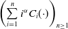 $\left (\sum \limits _{i=1}^n i^\alpha C_i({\cdot})\right )_{n\geq 1}$
on
$\left (\sum \limits _{i=1}^n i^\alpha C_i({\cdot})\right )_{n\geq 1}$
on $[0,T]$
.
$[0,T]$
.
To conclude, we only need to show that the solution constructed in the previous proof enjoys the additional property (3.3). As $U \in \mathcal{K}_1\cup \mathcal{K}_2$
, (3.3) follows from Lemma3.4 and the convergence (3.12).
$U \in \mathcal{K}_1\cup \mathcal{K}_2$
, (3.3) follows from Lemma3.4 and the convergence (3.12).
4. Uniqueness
We first need some estimates on a solution that satisfies (2.3). These are as follows:
Lemme 4.1.
A solution $C$
of (
1.1
) on
$C$
of (
1.1
) on $[0,T)$
which satisfy the condition (
2.3
) also satisfies, for all
$[0,T)$
which satisfy the condition (
2.3
) also satisfies, for all $t\in (0,T)$
,
$t\in (0,T)$
,
 \begin{equation} \lim _{n\to +\infty } \int _0^t n^\alpha a_n C_n(s)C_1(s)ds = 0, \end{equation}
 \begin{equation} \lim _{n\to +\infty } \int _0^t \sum _{i=n}^{+\infty } a_iC_i(s)C_1(s)ds = 0. \end{equation}
Proof. Let $n\geq 2$
and
$n\geq 2$
and $t\in (0,T)$
, recalling (H1), we have
$t\in (0,T)$
, recalling (H1), we have
 \begin{equation*} \int _0^t n^\alpha a_n C_1C_n ds \leq \int _0^t \sum _{i=n}^{+\infty } i^\alpha a_iC_i C_1 ds \leq a\int _0^t \sum _{i=n}^{+\infty } i^{2\alpha } C_i C_1 ds . \end{equation*}
and
 \begin{equation*} \int _0^t \sum _{i=n}^{+\infty } a_iC_i C_1 ds \leq a\int _0^t \sum _{i=n}^{+\infty } i^{2\alpha } C_i C_1 ds . \end{equation*}
Therefore, both assertions (4.1) and (4.2) come from Lebesgue-dominated convergence theorem using (2.4) and (2.3).
Proof of Theorem
2.4. Let $C=(C_i)_{i\geq 1}$
and
$C=(C_i)_{i\geq 1}$
and $D=(D_i)_{i\geq 1}$
denote two solutions of (1.1) on
$D=(D_i)_{i\geq 1}$
denote two solutions of (1.1) on $[0,T)$
with
$[0,T)$
with $C(0)=D(0)=C^{init}$
, which satisfy (2.3). For
$C(0)=D(0)=C^{init}$
, which satisfy (2.3). For $i\geq 1$
, defines
$i\geq 1$
, defines
 \begin{equation*} z_i \,:\!=\, C_i-D_i, \text{ and } g_i\,:\!=\,i^\alpha \,\text{sign}(z_i),\end{equation*}
where $\text{sign}$
denotes the sign function, i.e.
$\text{sign}$
denotes the sign function, i.e. $\text{sign}(x)=\frac {x}{|x|}$
for
$\text{sign}(x)=\frac {x}{|x|}$
for $x \in \mathbb{R}^*$
and
$x \in \mathbb{R}^*$
and $\text{sign}(0)=0$
. Now, we fix
$\text{sign}(0)=0$
. Now, we fix $n\geq 2$
, and
$n\geq 2$
, and $t\in (0,T)$
. The goal is to show that
$t\in (0,T)$
. The goal is to show that $\|z(t)\|_{X_\alpha } = 0$
, which will entail the desired uniqueness result.
$\|z(t)\|_{X_\alpha } = 0$
, which will entail the desired uniqueness result.
Note that if $f \in AC(\mathbb{R})$
, then
$f \in AC(\mathbb{R})$
, then $|f| \in AC(\mathbb{R})$
, and therefore
$|f| \in AC(\mathbb{R})$
, and therefore
 \begin{equation*} \frac {d}{dt}|f(t)| = \text{sign}(f(t))\frac {df}{dt}(t) \text{ a.e. in } \mathbb{R}. \end{equation*}
Since $C$
and
$C$
and $D$
are absolute continuous functions,
$D$
are absolute continuous functions, $z$
is also an absolute continuous function, and therefore, using the integral form of (1.1), we obtain
$z$
is also an absolute continuous function, and therefore, using the integral form of (1.1), we obtain
 \begin{align*} \sum _{i=1}^n i^\alpha |z_i(t)| & = \sum _{i=1}^n g_iz_i(t) = -\int _0^t \sum _{j=1}^{+\infty } g_1 a_j [C_1(s)C_j(s) - D_1(s)D_j(s)] + g_1a_1\big[C_1(s)^2-D_1(s)^2\big]ds \\ &\quad + \sum _{i=2}^n \int _0^t g_i a_{i-1}\left [C_{i-1}(s)C_1(s)-D_{i-1}(s)D_1(s)\right ]ds \\ &\quad -\sum _{i=2}^n \int _0^t g_i a_{i}\left [C_{i}(s)C_1(s)-D_{i}(s)D_1(s)\right ]ds \\ &\quad + \sum _{i=2}^n \left ( -\int _0^t g_ib_i\left [C_i(s)-D_i(s)\right ]ds + \int _0^t g_ib_{i+1}\left [C_{i+1}(s)-D_{i+1}(s)\right ]ds \right ) \\ &= \int _0^t \sum _{i=1}^{n-1} (g_{i+1}-g_i-g_1)a_i[C_i(s)C_1(s) - D_i(s)D_1(s)] ds \\ &\quad - \int _0^t g_{n}a_n[C_1(s)C_n(s)-D_1(s)D_n(s)] ds \\ &\quad - \sum _{i=n}^{+\infty } \int _0^t g_1 a_{i}\left [C_{i}(s)C_1(s)-D_{i}(s)D_1(s)\right ]ds \\ &\quad + \sum _{i=2}^n \left ( -\int _0^t g_ib_i\left [C_i(s)-D_i(s)\right ]ds + \int _0^t g_ib_{i+1}\left [C_{i+1}(s)-D_{i+1}(s)\right ]ds \right )\!. \end{align*}
However, $C_{i}(s)C_1(s)-D_{i}(s)D_1(s) = C_i(s)z_1(s)+D_1(s)z_i(s)$
, therefore
$C_{i}(s)C_1(s)-D_{i}(s)D_1(s) = C_i(s)z_1(s)+D_1(s)z_i(s)$
, therefore
 \begin{align*} \sum _{i=1}^n i^\alpha |z_i(t)| &\leq \int _0^t \sum _{i=1}^{n-1} (g_{i+1}-g_i-g_1)a_i[C_i(s)z_1(s) + z_i(s)D_1(s)] ds \\ & \quad - \int _0^t g_{n}a_n[C_1(s)C_n(s)-D_1(s)D_n(s)] ds \\ &\quad - \sum _{i=n}^{+\infty } \int _0^t g_1 a_{i}\left [C_{i}(s)C_1(s)-D_{i}(s)D_1(s)\right ]ds \\ &\quad + \sum _{i=2}^n \left ( -\int _0^t g_ib_i\left [C_i(s)-D_i(s)\right ]ds + \int _0^t g_ib_{i+1}\left [C_{i+1}(s)-D_{i+1}(s)\right ]ds \right )\!. \end{align*}
As $\text{sign}(x) \leq 1$
for all
$\text{sign}(x) \leq 1$
for all $x\in \mathbb{R}$
, we have for all
$x\in \mathbb{R}$
, we have for all $i,j\geq 1$
,
$i,j\geq 1$
,
 \begin{align} (g_{i+j}-g_i-g_j)z_j &= ((i+j)^\alpha \text{sign}(z_{i+j})-i^\alpha \text{sign}(z_i)-j^\alpha \text{sign}(z_j))z_j \nonumber\\ &= ((i+j)^\alpha \text{sign}(z_{i+j}z_j)-i^\alpha \text{sign}(z_iz_j)-j^\alpha )|z_j| \nonumber\\ &\leq ((i+j)^\alpha + i^\alpha - j^\alpha )|z_j| \nonumber\\ &\leq 2i^\alpha |z_j|. \end{align}
Moreover, using (H1), we obtain
 \begin{align*} \sum _{i=2}^n \left ( -\int _0^t g_ib_iz_i(s)ds + \int _0^t g_ib_{i+1}z_{i+1}(s)ds \right ) &= \int _0^t \sum _{i=2}^{n-1} g_{i-1}b_iz_i(s) - \sum _{i=2}^ng_ib_iz_i(s) ds \\ &= -\int _0^t \sum _{i=2}^{n-1} (g_{i}-g_{i-1})b_iz_i(s) ds - \int _0^t \underbrace {n^\alpha b_n|z_n(s)|}_{\geq 0}ds. \end{align*}
However, $(g_i-g_{i-1})z_i = (i^\alpha -(i-1)^\alpha \text{sign}(z_{i-1}z_i))|z_i| \geq 0$
, this entails that
$(g_i-g_{i-1})z_i = (i^\alpha -(i-1)^\alpha \text{sign}(z_{i-1}z_i))|z_i| \geq 0$
, this entails that
 \begin{equation} \sum _{i=2}^n \left ( -\int _0^t g_ib_iz_i(s)ds + \int _0^t g_ib_{i+1}z_{i+1}(s)ds \right ) \leq 0. \end{equation}
Therefore, using (4.3) and (4.4), we have
 \begin{align} \sum _{i=1}^n i^\alpha |z_i(t)| &\leq \int _0^t \sum _{i=1}^{n-1} a_i i^\alpha |z_1(s)|C_i(s) +\sum _{i=1}^{n-1} a_i |z_i(s)|D_1(s)ds \nonumber\\ & \quad - \int _0^t g_{n}a_n[C_1(s)C_n(s)-D_1(s)D_n(s)] ds \nonumber\\ &\quad - \int _0^t \sum _{i=n}^{+\infty } g_1 a_{i}\left [C_{i}(s)C_1(s)-D_{i}(s)D_1(s)\right ]ds. \end{align}
We now treat one by one the three terms on the right-hand side of the above inequality.
First term: Using (H1), we have
 \begin{align*} \int _0^t \sum _{i=1}^{n-1} a_i i^\alpha |z_1(s)|C_i(s) ds &+ \int _0^t \sum _{i=1}^{n-1} a_i |z_i(s)|D_1(s)ds \\ &\leq \int _0^t \sum _{i=1}^n i^\alpha a_i C_i(s) \sum _{i=1}^n |z_i(s)| + \sum _{i=1}^n a_i|z_i(s)| \sum _{i=1}^n i^\alpha D_i(s) ds \\ &\leq \int _0^t \left ( \sum _{i=1}^{n} i^\alpha a_i C_i(s) + a \sum _{i=1}^n i^\alpha D_i(s) \right )\sum _{i=1}^n i^\alpha |z_i(s)| ds. \end{align*}
Using (2.3) and Lebesgue-dominated convergence theorem, we obtain
 \begin{align} &\lim _{n\to +\infty } \int _0^t \sum _{i=1}^{n-1} a_i i^\alpha |z_1(s)|C_i(s) +\sum _{i=1}^{n-1} a_i |z_i(s)|D_1(s)ds \nonumber \\ &\quad \leq \int _0^t \left ( \sum _{i=1}^{+\infty } i^\alpha a_i C_i(s) + a \big(\lambda T + \|C^{init}\|_{X_\alpha }\big) \right )\sum _{i=1}^{+\infty } i^\alpha |z_i(s)| ds. \end{align}
Second term: As $-g_n[C_1C_n-D_1D_n] \leq n^\alpha [C_1C_n+D_1D_n]$
, we have
$-g_n[C_1C_n-D_1D_n] \leq n^\alpha [C_1C_n+D_1D_n]$
, we have
 \begin{align*} - \int _0^t g_{n}a_n[C_1(s)C_n(s)-D_1(s)D_n(s)] ds \leq \int _0^t n^\alpha a_n C_1(s)C_n(s) ds + \int _0^t n^\alpha a_n D_1(s)D_n(s) ds. \end{align*}
Using (H1) and (4.1) from Lemma4.1, we obtain
 \begin{equation} \lim _{n\to +\infty } - \int _0^t g_{n}a_n[C_1(s)C_n(s)-D_1(s)D_n(s)] ds = 0. \end{equation}
Third term: We have
 \begin{equation*} - \int _0^t \sum _{i=n}^{+\infty } g_1 a_{i}\left [C_{i}(s)C_1(s)-D_{i}(s)D_1(s)\right ]ds \leq \int _0^t \sum _{i=n}^{+\infty } a_iC_1(s)C_i(s) ds + \int _0^t \sum _{i=n}^{+\infty } a_iD_1(s)D_i(s)ds. \end{equation*}
Therefore, using (4.2) from Lemma4.1, we obtain
 \begin{equation} \lim _{n\to +\infty } - \int _0^t \sum _{i=n}^{+\infty } g_1 a_{i}\left [C_{i}(s)C_1(s)-D_{i}(s)D_1(s)\right ]ds = 0. \end{equation}
Passing to the limit $n\to +\infty$
in (4.5), the previous estimations (4.6)–(4.8) entail that
$n\to +\infty$
in (4.5), the previous estimations (4.6)–(4.8) entail that
 \begin{equation*} \sum _{i=1}^{+\infty } i^\alpha |z_i(t)| \leq \int _0^t \left ( \sum _{i=1}^{+\infty } i^\alpha a_i C_i(s) + a \big(\lambda T + \|C^{init}\|_{X_\alpha }\big) \right )\sum _{i=1}^{+\infty } i^\alpha |z_i(s)| ds. \end{equation*}
Then, applying Grönwall’s lemma, we obtain that for all $t\in [0,T)$
,
$t\in [0,T)$
,
 \begin{equation*} \sum _{i=1}^{+\infty } i^\alpha |z_i(t)| \leq 0, \end{equation*}
which entails $C=D$
and ends the proof.
$C=D$
and ends the proof.
5. Long-time behaviour
5.1. Uniform-in-time bound
We start by proving Proposition2.6.
Proof of Proposition
2.6. Let $M\gt 1$
, for convenience, we rewrite condition (2.6) as
$M\gt 1$
, for convenience, we rewrite condition (2.6) as
 \begin{equation} \frac {b_i}{a_i} \geq M\kappa \text{ for all } i\geq 1. \end{equation}
Let $t\geq 0$
and
$t\geq 0$
and $\mu \in (1,M)$
. We have the following formal computations:
$\mu \in (1,M)$
. We have the following formal computations:
 \begin{align*} \frac {d}{dt}\sum _{i=1}^{+\infty }\mu ^iC_i(t) &= \mu \left (\lambda - \sum _{j=1}^{+\infty }a_jC_j(t)C_1(t)-a_1C_1(t)^2\right ) + \sum _{i=2}^{+\infty }\mu ^i(J_{i-1}(t)-J_i(t)) \\ &= \mu \left (\lambda - \sum _{j=1}^{+\infty }a_jC_j(t)C_1(t)-a_1C_1(t)^2\right ) + (\mu - 1)\sum _{i=1}^{+\infty }\mu ^iJ_i + \mu (a_1C_1(t)^2-b_2C_2(t)) \\ &\leq \mu \lambda - \mu a_1C_1(t)^2 + (\mu -1)\sum _{i=1}^{+\infty }\mu ^i(a_iC_i(t)C_1(t)-b_{i+1}C_{i+1}(t)) + \mu (a_1C_1(t)^2-b_2C_2(t)) \\ &= \mu \lambda + (\mu -1)\sum _{i=1}^{+\infty }\mu ^{i-1}a_i\left (\mu C_1(t)-\frac {b_i}{a_i}\right )C_i(t) +(\mu -1)b_1C_1(t) - \mu b_2C_2(t) \\ &= \mu \lambda + \frac {(\mu -1)}{\mu }\sum _{i=1}^{+\infty }\mu ^{i}a_i\left (\mu C_1(t)-\frac {b_i}{a_i}\right )C_i(t) +(\mu -1)b_1C_1(t) - \mu b_2C_2(t) \\ &\leq \mu \lambda +(\mu -1)b_1C_1(t) + \frac {(\mu -1)}{\mu }\sum _{i=1}^{+\infty }\mu ^{i}a_i\left (\mu C_1(t)-\frac {b_i}{a_i}\right )C_i(t). \end{align*}
Then, using (2.4) and (5.1) and denoting $\varepsilon = (M-\mu )\kappa \gt 0$
, we have
$\varepsilon = (M-\mu )\kappa \gt 0$
, we have
 \begin{align*} \frac {d}{dt}\sum _{i=1}^{+\infty }\mu ^iC_i(t) &\leq \mu \lambda + (\mu -1)b_1\kappa - \varepsilon \frac {\mu -1}{\mu }\sum _{i=1}^{+\infty }a_i\mu ^iC_i(t) \\ &\leq \mu \lambda + (\mu -1)b_1\kappa - \varepsilon \frac {\mu -1}{\mu }\underline {a}\sum _{i=1}^{+\infty }\mu ^iC_i(t). \end{align*}
Therefore, using Grönwall’s lemma, we obtain for all $t\geq 0$
and
$t\geq 0$
and $\mu \in (1,M)$
,
$\mu \in (1,M)$
,
 \begin{equation*} \sum _{i=1}^{+\infty }\mu ^iC_i(t) \leq \sum _{i=1}^{+\infty }\mu ^iC_i^{init} + \frac {\lambda \mu +(\mu -1)b_1\kappa }{\varepsilon \frac {\mu -1}{\mu }\underline {a}} \,:\!=\, \Xi _1, \end{equation*}
where $\Xi _1$
depends only on
$\Xi _1$
depends only on $\lambda$
,
$\lambda$
, $(a_i)_{i\geq 1}$
,
$(a_i)_{i\geq 1}$
, $(b_i)_{i\geq 1}$
,
$(b_i)_{i\geq 1}$
, $\mu$
and the initial condition. Taking
$\mu$
and the initial condition. Taking $\nu = \ln (\mu )$
, we have the desired estimation (2.8).
$\nu = \ln (\mu )$
, we have the desired estimation (2.8).
The rigorous proof can be left to the reader, as it consists in reproducing these estimates on the truncated system (2.16), (3.4) and then letting $n\to +\infty$
using
$n\to +\infty$
using $C_i^n \to C_i$
and
$C_i^n \to C_i$
and $\sum _{i=1}^n \mu ^iC_i^n \to \sum _{i=1}^{+\infty } \mu ^iC_i$
.
$\sum _{i=1}^n \mu ^iC_i^n \to \sum _{i=1}^{+\infty } \mu ^iC_i$
.
As mention in the beginning, we have an upper bound on the mass and lower bound on $C_1(t)$
.
$C_1(t)$
.
Proposition 5.1 (Mass uniform-in-time bound). Let $b\gt 0$
. Assume that
$b\gt 0$
. Assume that $C^{init} \in X_1^+$
and that the kinetics coefficients satisfy the following conditions:
$C^{init} \in X_1^+$
and that the kinetics coefficients satisfy the following conditions:
 \begin{equation} \forall i\geq 1,\, b_i\geq bi. \end{equation}
Then, for all $t\geq 0$
,
$t\geq 0$
,
 \begin{equation} \sum _{i=1}^{+\infty } iC_i(t) \leq \max \left \{\sum _{i=1}^{+\infty } iC_i^{init}, \frac {\lambda + b_1\kappa }{b}\right \}\!. \end{equation}
Proof of Proposition
5.1. Recalling (2.1) and using the assumption (5.2) and the uniform-in-time bound of $C_1$
(2.4), we have for all
$C_1$
(2.4), we have for all $t\geq 0$
,
$t\geq 0$
,
 \begin{align*} \frac {d}{dt}\sum _{i=1}^{+\infty }iC_i(t) &= \lambda -b_2C_2 - \sum _{i=2}^{+\infty }b_iC_i \\ &\leq \lambda -2bC_2+b_1C_1-b\sum _{i=1}^{+\infty }iC_i \\ &\leq \lambda + b_1\kappa - b\sum _{i=1}^{+\infty } iC_i. \end{align*}
Therefore, for all $t\geq 0$
,
$t\geq 0$
,
 \begin{equation*} \sum _{i=1}^{+\infty }iC_i(t) \leq \max \left \{\sum _{i=1}^{+\infty } iC_i^{init}, \frac {\lambda + b_1\kappa }{b}\right \}\!. \end{equation*}
Proposition 5.2 ( ${{C}}_{1}$
uniform-in-time positivity). Let
${{C}}_{1}$
uniform-in-time positivity). Let $a,b\gt 0$
. Assume that the kinetics coefficients satisfy the following conditions:
$a,b\gt 0$
. Assume that the kinetics coefficients satisfy the following conditions:
 \begin{equation} \forall i\geq 1,\, a_i\leq ai \,\text{ and }\, b_i\geq bi. \end{equation}
Then, there exists a constant $\eta \gt 0$
and
$\eta \gt 0$
and $t_1 \geq 0$
such that for all
$t_1 \geq 0$
such that for all $t\geq t_1$
, we have
$t\geq t_1$
, we have
 \begin{equation} C_1(t) \geq \eta . \end{equation}
Proof of Proposition
5.2. First, using (5.4) and the uniform-in-time bound of the mass (5.3), we have for all $t\geq 0$
,
$t\geq 0$
,
 \begin{equation*} \sum _{i=1}^{+\infty }a_iC_i(t) \leq a \sum _{i=1}^{+\infty }iC_i(t) \leq a \max \left \{\sum _{i=1}^{+\infty }iC_i^{init},\frac {\lambda +b_1\kappa }{b}\right \}\!. \end{equation*}
Then, for all $t\geq 0$
, we have
$t\geq 0$
, we have
 \begin{align*} \frac {d}{dt}C_1(t) &= \lambda - \sum _{j=1}^{+\infty }a_jC_j(t)C_1(t) - a_1C_1(t)^2 \\ &\geq \lambda - a \max \left \{\sum _{i=1}^{+\infty }iC_i^{init},\frac {\lambda +b_1\kappa }{b}\right \}C_1(t) - a_1C_1(t)^2. \end{align*}
Therefore, as long as $C_1 \leq \min \left \{ 1,a \max \left \{\sum \limits _{i=1}^{+\infty }iC_i^{init},\frac {\lambda +b_1\kappa }{b}\right \} +a \right \}$
, we have
$C_1 \leq \min \left \{ 1,a \max \left \{\sum \limits _{i=1}^{+\infty }iC_i^{init},\frac {\lambda +b_1\kappa }{b}\right \} +a \right \}$
, we have
 \begin{align*} \frac {d}{dt}C_1(t) &\geq \lambda - \left [ a \max \left \{\sum _{i=1}^{+\infty }iC_i^{init},\frac {\lambda +b_1\kappa }{b}\right \} + a_1\right ] C_1(t)\\ &\geq \lambda - \left [ a \max \left \{\sum _{i=1}^{+\infty }iC_i^{init},\frac {\lambda +b_1\kappa }{b}\right \} + a\right ] C_1(t) \geq 0. \end{align*}
Hence, there exists $t_1 \geq 0$
such that for all
$t_1 \geq 0$
such that for all $t\geq t_1$
,
$t\geq t_1$
,
 \begin{equation*} C_1(t) \geq \frac {1}{2} \min \left \{ 1, a \max \left \{\sum _{i=1}^{+\infty }iC_i^{init},\frac {\lambda +b_1\kappa }{b}\right \} + a \right \} \,=\!:\, \eta . \end{equation*}
5.2. Steady states
In this subsection, we prove Theorem2.9. Let $C=(C_i)_{i\geq 1}$
a constant solution. From (1.1), we obtain
$C=(C_i)_{i\geq 1}$
a constant solution. From (1.1), we obtain
 \begin{equation*} J_{i-1} = J_i, \,\forall i \geq 2. \end{equation*}
Therefore, there exists $J \in \mathbb{R}$
such that
$J \in \mathbb{R}$
such that
 \begin{equation} J_i = J, \,\forall i\geq 1. \end{equation}
We then have three possibilities: either $J=0$
, or
$J=0$
, or $J \gt 0$
or
$J \gt 0$
or $J\lt 0$
. We immediately obtain that there is no steady state with a positive flux
$J\lt 0$
. We immediately obtain that there is no steady state with a positive flux $J\gt 0$
. Indeed, from (H1) and the positivity of solutions, we have
$J\gt 0$
. Indeed, from (H1) and the positivity of solutions, we have
 \begin{equation*} a_iC_1C_i = J + b_{i+1}C_{i+1} \geq J. \end{equation*}
Therefore,
 \begin{equation*} \sum _{i=1}^{+\infty }a_iC_1C_i \geq \sum _{i=1}^{+\infty }J = +\infty , \end{equation*}
which means that there is no steady state when $J\gt 0$
due to the equation on
$J\gt 0$
due to the equation on $C_1$
.
$C_1$
.
The case $J=0$
gives the steady-state
$J=0$
gives the steady-state $(Q_iz^i)_{i\geq 1}$
. Assuming that a steady state exists, we denote it
$(Q_iz^i)_{i\geq 1}$
. Assuming that a steady state exists, we denote it $C^{eq}$
, the equation (5.6) entails the following relation:
$C^{eq}$
, the equation (5.6) entails the following relation:
 \begin{equation*} a_iC_1^{eq}C_i^{eq} = b_{i+1}C_{i+1}^{eq}, \,\forall i\geq 1. \end{equation*}
Thus,
 \begin{equation*} C_i^{eq} = \left (\prod _{j=2}^{i} \frac {a_{j-1}}{b_j}\right )\big(C_1^{eq}\big)^i = Q_i\big(C_1^{eq}\big)^i, \,\forall i\geq 1. \end{equation*}
The steady state is therefore entirely determined by $C_1^{eq}$
; to determine this value, we use the first equation of the system (1.1), which has not yet been used. We, therefore, have that
$C_1^{eq}$
; to determine this value, we use the first equation of the system (1.1), which has not yet been used. We, therefore, have that $C_1^{eq}$
is a solution of the following equation in
$C_1^{eq}$
is a solution of the following equation in $z$
$z$
 \begin{equation} \lambda = \sum _{j=1}^{+\infty }a_{j}Q_jz^{j+1} + a_1 z^2. \end{equation}
By comparing with the critical production threshold $\lambda _s$
defined in (2.10), the equation (5.7) admits a unique solution when
$\lambda _s$
defined in (2.10), the equation (5.7) admits a unique solution when $\lambda \leq \lambda _s$
, which verifies
$\lambda \leq \lambda _s$
, which verifies $z \leq z_s$
.
$z \leq z_s$
.
The last case is the negative flux $J\lt 0$
. Using equation (5.6), we have
$J\lt 0$
. Using equation (5.6), we have
 \begin{equation} J(z) \,:\!=\, a_izg_i(z) - b_{i+1}g_{i+1}(z), \,\, \forall i\geq 1, \end{equation}
where $z$
and functions
$z$
and functions $g_i(z)$
designate a constant solution. In other words, we search for a steady state
$g_i(z)$
designate a constant solution. In other words, we search for a steady state
 \begin{equation*} C_i = g_i(z), \end{equation*}
for all $i\geq 1$
, with
$i\geq 1$
, with $g_1(z) = z$
.
$g_1(z) = z$
.
We now want to determine $J$
and the
$J$
and the $g_i$
functions. To do this, we start from (5.8), divide the two members of this equality by
$g_i$
functions. To do this, we start from (5.8), divide the two members of this equality by $a_iQ_iz^{i+1}$
, and using (2.9), we obtain
$a_iQ_iz^{i+1}$
, and using (2.9), we obtain
 \begin{equation} \frac {J(z)}{a_iQ_iz^{i+1}} = \frac {a_izg_i(z)}{a_iQ_iz^{i+1}} - \frac {b_{i+1}g_{i+1}(z)}{a_iQ_iz^{i+1}} = \frac {g_i(z)}{Q_iz^i} - \frac {g_{i+1}(z)}{Q_{i+1}z^{i+1}} \end{equation}
Summing from $i=1$
to
$i=1$
to $k-1$
, we obtain
$k-1$
, we obtain
 \begin{equation} J(z)\sum _{i=1}^{k-1} \frac {1}{a_iQ_iz^{i+1}} = 1 - \frac {g_k(z)}{Q_kz^k}. \end{equation}
Rewriting (5.10), we obtain the expression of $g_k(z)$
for all
$g_k(z)$
for all $k\geq 2$
:
$k\geq 2$
:
 \begin{equation} g_k(z) = Q_kz^k\left [ 1 - J(z)\sum _{i=1}^{k-1}\frac {1}{a_iQ_iz^{i+1}} \right ]\!, \end{equation}
and we also find $g_1(z) = z$
.
$g_1(z) = z$
.
In order for the sequence $(g_k(z))_{k\geq 1}$
to be a steady state, it needs to be summable against
$(g_k(z))_{k\geq 1}$
to be a steady state, it needs to be summable against $(a_k)_{k\geq 1}$
. We have
$(a_k)_{k\geq 1}$
. We have
 \begin{equation*} \sum _{k=2}^{+\infty }a_kg_k(z) = \sum _{k=2}^{+\infty } a_kQ_kz^k - J(z)\sum _{k=2}^{+\infty }a_kQ_kz_k\left (\sum _{i=1}^{k-1}\frac {1}{a_iQ_iz^{i+1}}\right )\!. \end{equation*}
From the definition of $z_s$
as the radius of convergence of a power series, we observe that if
$z_s$
as the radius of convergence of a power series, we observe that if $z\gt z_s$
, then the series
$z\gt z_s$
, then the series $\sum a_kQ_kz^k$
is divergent; therefore, there is no steady state in the super-critical case. We now suppose that
$\sum a_kQ_kz^k$
is divergent; therefore, there is no steady state in the super-critical case. We now suppose that $z\leq z_s$
. We have for all
$z\leq z_s$
. We have for all $k\geq 1$
,
$k\geq 1$
,
 \begin{align} a_kg_k(z) = a_kQ_kz^k\left [ 1 - J(z) \sum _{i=1}^{k-1}\frac {1}{a_iQ_iz^{i+1}} \right ] &\gt |J(z)|a_kQ_kz_k\sum _{i=1}^{k-1}\frac {1}{a_iQ_iz^{i+1}} \nonumber\\ &= |J(z)| \frac {a_k}{b_k} + \sum _{i=1}^{k-2}\frac {a_kQ_k}{a_iQ_i}z^{k-(i+1)} \end{align}
Therefore, using (H3) and (H4), if $z_s\lt +\infty$
, then
$z_s\lt +\infty$
, then $a_kg_k(z)$
does not converge towards 0, and therefore, the series diverge. This implies that there is no steady state in the super-critical case, and no other steady state in the sub-critical case when
$a_kg_k(z)$
does not converge towards 0, and therefore, the series diverge. This implies that there is no steady state in the super-critical case, and no other steady state in the sub-critical case when $z_s$
is finite.
$z_s$
is finite.
It remains to prove the uniqueness of the steady state or the existence of an infinite number of steady-state depending on the comparison of the kinetics rates.
First case: $b_i \leq i a_i$
for
$b_i \leq i a_i$
for $i \gg 1$
. Recalling the expression (5.11), we show that in this case they are not summable against
$i \gg 1$
. Recalling the expression (5.11), we show that in this case they are not summable against $(a_k)_{k\geq 1}$
. Let
$(a_k)_{k\geq 1}$
. Let $h(x)=\sum _{k=1}^{+\infty } a_kQ_kx^k$
for
$h(x)=\sum _{k=1}^{+\infty } a_kQ_kx^k$
for $x\in [0,z_s)$
; noticing that all derivatives of
$x\in [0,z_s)$
; noticing that all derivatives of $h$
are increasing in
$h$
are increasing in $x$
and using (2.9), we have
$x$
and using (2.9), we have
 \begin{align*} \sum _{k=2}^{+\infty } a_kg_k(z) &\geq |J|\sum _{k=2}^{+\infty }a_kQ_kz^k\sum _{i=1}^{k-1}\frac {1}{a_iQ_iz^{i+1}} = |J|\sum _{i=2}^{+\infty } \frac {1}{a_iQ_iz^{i+1}}\sum _{k=i+1}^{+\infty }a_kQ_kz^k \\ &= |J|\sum _{i=2}^{+\infty } \frac {1}{a_iQ_iz^{i+1}}\int _0^z h^{(i+1)}(t)\frac {(z-t)^i}{i!}dt \geq \frac {|J|}{z} \sum _{i=2}^{+\infty } \frac {1}{a_iQ_iz^i}\frac {h^{(i+1)}(0)}{i!} \int _0^z (z-t)^i dt \\ &= \frac {|J|}{z}\sum _{i=2}^{+\infty } \frac {(i+1)a_{i+1}}{b_{i+1}} \int _0^z \left (1-\frac {t}{z}\right )^i dt = |J|\sum _{i=2}^{+\infty } \frac {a_{i+1}}{b_{i+1}} \\ &\geq |J|\sum _{i=2}^{+\infty } \frac {1}{i} = +\infty . \end{align*}
Which proves that in this case, there is no other steady state.
Second case: $b_i \gt i^\nu a_i$
for
$b_i \gt i^\nu a_i$
for $i\gg 1$
with
$i\gg 1$
with $\nu \gt 1$
. Using the relation (5.6), we obtain for
$\nu \gt 1$
. Using the relation (5.6), we obtain for $J\lt 0$
 \begin{equation*} C_{i+1} = \frac {a_izC_i+|J|}{b_{i+1}} \,\forall i\geq 1 \text{ and } C_1 = z. \end{equation*}
Solving the recurring sequence, we obtain for $i\geq 2$
 \begin{equation*} C_i = |J|\sum _{k=0}^{i-2} \frac {Q_i}{a_{i-1-k}Q_{i-1-k}}z^k + Q_iz^i. \end{equation*}
First, we prove that this sequence is summable against $(a_i)_{i\geq 1}$
. Since
$(a_i)_{i\geq 1}$
. Since $\sum a_iQ_iz^i$
is finite for
$\sum a_iQ_iz^i$
is finite for $z\lt z_s$
, it remains to prove that the first term is summable against
$z\lt z_s$
, it remains to prove that the first term is summable against $(a_i)_{i\geq 1}$
. We have
$(a_i)_{i\geq 1}$
. We have
 \begin{equation*} \sum _{i=1}^{+\infty }a_i\sum _{k=0}^{i-2} \left (\frac {Q_i}{a_{i-1-k}Q_{i-1-k}}\right )z^k = \sum _{k=0}^{+\infty } \sum _{i=k+2}^{+\infty } \frac {a_iQ_i}{a_{i-1-k}Q_{i-1-k}}z^k = \sum _{k=0}^{+\infty } \underbrace {\left [\sum _{j=2}^{+\infty }\frac {a_{j+k}Q_{j+k}}{a_{j-1}Q_{j-1}}\right ]}_{\,:\!=\, \gamma _k}z^k \end{equation*}
For all $k\geq 0$
, we prove that
$k\geq 0$
, we prove that $\gamma _k \lt +\infty$
. Let
$\gamma _k \lt +\infty$
. Let $k\geq 0$
, there exists
$k\geq 0$
, there exists $j_0 \gg 1$
such that for
$j_0 \gg 1$
such that for $j\geq j_0$
we have
$j\geq j_0$
we have $Q_{j+k} \leq Q_j$
. Thus, using (H4), the sequence of ratio is bounded by
$Q_{j+k} \leq Q_j$
. Thus, using (H4), the sequence of ratio is bounded by $K \geq 0$
and the hypothesis of the second case, we have
$K \geq 0$
and the hypothesis of the second case, we have
 \begin{equation*} \sum _{j\geq j_0} \frac {a_{j+k}Q_{j+k}}{a_{j-1}Q_{j-1}} \leq \sum _{j\geq j_0} \frac {a_{j+k}Q_{j}}{a_{j-1}Q_{j-1}} = \sum _{j\geq j_0} \frac {a_{j+k}}{b_j} \leq \sum _{j\geq j_0} \frac {a_{j+k}}{j^\nu a_j} \leq K^{k+1} \sum _{j\geq j_0} \frac {1}{j^\nu } \lt +\infty . \end{equation*}
This is where the hypothesis of the second case, mainly $\nu \gt 1$
, is crucial. Otherwise,
$\nu \gt 1$
, is crucial. Otherwise, $\gamma _k = +\infty$
and the computation does not allow us to conclude. Computing the ratio of
$\gamma _k = +\infty$
and the computation does not allow us to conclude. Computing the ratio of $\gamma _k$
, we have
$\gamma _k$
, we have
 \begin{align*} \frac {\gamma _{k+1}}{\gamma _k} = \frac {\sum \limits _{j=2}^{+\infty }\dfrac {a_{j+k+1}Q_{j+k+1}}{a_{j-1}Q_{j-1}}}{\sum \limits _{j=2}^{+\infty }\dfrac {a_{j+k}Q_{j+k}}{a_{j-1}Q_{j-1}}} = \frac {\sum \limits _{j=2}^{+\infty }\dfrac {a_{j+k}Q_{j+k}}{a_{j-1}Q_{j-1}}\dfrac {a_{j+k+1}}{b_{j+k+1}}}{\sum \limits _{j=2}^{+\infty }\dfrac {a_{j+k}Q_{j+k}}{a_{j-1}Q_{j-1}}}. \end{align*}
However, for $k\gg 1$
using the hypothesis of the second case, we have
$k\gg 1$
using the hypothesis of the second case, we have
 \begin{equation*} \frac {a_{j+k+1}}{b_{j+k+1}} \lt \frac {a_{j+k+1}}{(j+k+1)^\nu a_{j+k+1}} \lt \frac {1}{(k+1)^\nu }. \end{equation*}
Therefore,
 \begin{equation*} \frac {\gamma _{k+1}}{\gamma _k} \leq \frac {1}{(k+1)^\nu } \xrightarrow {k\to +\infty } 0. \end{equation*}
Using D’Alembert’s ratio test, the sum $\sum a_iC_i$
converges for all
$\sum a_iC_i$
converges for all $z\geq 0$
. To obtain a steady state, it remains to satisfy the first equation and if there is any condition on
$z\geq 0$
. To obtain a steady state, it remains to satisfy the first equation and if there is any condition on $\lambda$
,
$\lambda$
, $z$
or
$z$
or $J$
. The equation
$J$
. The equation
 \begin{equation*} a_1 z^2 + z |J| \sum _{k=0}^{+\infty } \gamma _k z^k + \sum _{k=1}^{\infty } a_kQ_kz^{k+1} = \lambda \end{equation*}
admits, for all $J\lt 0$
, a unique
$J\lt 0$
, a unique $z$
such that the above equation is satisfied, since the left-hand side of the equation is a strictly increasing function of
$z$
such that the above equation is satisfied, since the left-hand side of the equation is a strictly increasing function of $z$
from 0 to
$z$
from 0 to $+\infty$
. We, therefore, obtain an infinity of steady states parameterised by
$+\infty$
. We, therefore, obtain an infinity of steady states parameterised by $J$
.
$J$
.
Remark 5.3. Note that every sequence, even increasing sequence, cannot be compared in the previous two cases. However, both cases already show the critical point at which the existence of a unique or of multiple steady states changes drastically. In the case of power law coefficients, the two cases are exhaustive.
5.3. Local exponential stability: Sub-critical case
Let $\Theta _i = Q_iz^i$
for all
$\Theta _i = Q_iz^i$
for all $i\geq 1$
. We introduce the ansatz
$i\geq 1$
. We introduce the ansatz $C_i = \Theta _i(1+h_i)$
where
$C_i = \Theta _i(1+h_i)$
where $h_i$
denotes the fluctuation around
$h_i$
denotes the fluctuation around $\Theta _i$
. We introduce the Hilbert space
$\Theta _i$
. We introduce the Hilbert space $\mathcal{H} \,:\!=\, \ell ^2(\Theta _i)$
and a subspace
$\mathcal{H} \,:\!=\, \ell ^2(\Theta _i)$
and a subspace $\mathcal{H}_{\mathcal{D}} = \ell ^2(\Theta _i(1+\sigma _i^2))$
namely
$\mathcal{H}_{\mathcal{D}} = \ell ^2(\Theta _i(1+\sigma _i^2))$
namely
 \begin{equation*} \mathcal{H} = \left \{ h = (h_i)_{i\geq 1} \;:\; \|h\|_{\mathcal{H}} \,:\!=\, \left (\sum _{i=1}^{+\infty } \Theta _ih_i^2\right )^{1/2} \lt \infty \right \}\!, \end{equation*}
and
 \begin{equation*} \mathcal{H}_{\mathcal{D}} = \left \{ h = (h_i)_{i\geq 1} \;:\; \|h\|_{\mathcal{H}_{\mathcal{D}}} \,:\!=\, \left (\sum _{i=1}^{+\infty } \Theta _i(1+\sigma _i^2)h_i^2\right )^{1/2} \lt \infty \right \}\!, \end{equation*}
where the sequence $(\sigma _i)_{i\geq 1}$
is defined later in (5.19). The inner scalar product of
$(\sigma _i)_{i\geq 1}$
is defined later in (5.19). The inner scalar product of $\mathcal{H}$
is denoted by
$\mathcal{H}$
is denoted by $\langle \cdot ,\cdot \rangle _{\mathcal{H}}$
. We define two linear operators
$\langle \cdot ,\cdot \rangle _{\mathcal{H}}$
. We define two linear operators $S$
and
$S$
and $P$
on
$P$
on $\mathcal{H}$
by the following weak form
$\mathcal{H}$
by the following weak form
 \begin{equation} \sum _{i=1}^{+\infty } S_i(h)\Theta _i\varphi _i = \sum _{i=1}^{+\infty } [\varphi _{i+1}-\varphi _i-\varphi _1]a_i\Theta _1\Theta _i(h_i+h_1-h_{i+1}), \end{equation}
and
 \begin{equation} \sum _{i=1}^{+\infty } P_i(h)\Theta _i\varphi _i = - \varphi _1\left (a_1\Theta _1^2h_2+\sum _{i=1}^{+\infty }a_i\Theta _1\Theta _ih_{i+1}\right )\!, \end{equation}
for any compactly supported sequences $(h_i)_{i\geq 1}$
and
$(h_i)_{i\geq 1}$
and $(\varphi _i)_{i\geq 1}$
. We denote by
$(\varphi _i)_{i\geq 1}$
. We denote by $L$
the sum of the previous operators, namely
$L$
the sum of the previous operators, namely
 \begin{equation} L = S + P. \end{equation}
We also define a bilinear operator $\Gamma$
by the following weak form
$\Gamma$
by the following weak form
 \begin{equation*} \sum _{i=1}^{+\infty } \Gamma _i(f,g)\Theta _i\varphi _i = \frac {1}{2}\sum _{i=1}^{+\infty }a_i\Theta _1\Theta _i(f_1g_i+f_ig_1)(\varphi _{i+1}-\varphi _i-\varphi _1), \end{equation*}
for any compactly supported sequences $(f_i)_{i\geq 1}$
,
$(f_i)_{i\geq 1}$
, $(g_i)_{i\geq 1}$
, and
$(g_i)_{i\geq 1}$
, and $(\varphi _i)_{i\geq 1}$
. We note that
$(\varphi _i)_{i\geq 1}$
. We note that $\Gamma (0,0)=0$
.
$\Gamma (0,0)=0$
.
The fluctuation $h$
satisfies
$h$
satisfies
 \begin{equation} \frac {d}{dt}h_i(t) = L_i(h(t)) + \Gamma _i(h(t),h(t)). \end{equation}
The aforementioned decomposition of the linear operator $L$
is due to the fact that the operator
$L$
is due to the fact that the operator $S$
is the linear operator studied by Cañizo and Lods [Reference Cañizo and Lods15] for the Becker–Döring equations. Consequently, it is established that
$S$
is the linear operator studied by Cañizo and Lods [Reference Cañizo and Lods15] for the Becker–Döring equations. Consequently, it is established that $S$
is a symmetric operator in
$S$
is a symmetric operator in $\mathcal{H}$
and dissipative. Cañizo and Lods proved that the operator
$\mathcal{H}$
and dissipative. Cañizo and Lods proved that the operator $S$
admits a spectral gap in
$S$
admits a spectral gap in $\mathcal{H}$
, and they have also proved a lower bound on this spectral gap. In order to prove that the steady state is then locally exponentially stable, it is necessary to establish estimates on the quadratic term
$\mathcal{H}$
, and they have also proved a lower bound on this spectral gap. In order to prove that the steady state is then locally exponentially stable, it is necessary to establish estimates on the quadratic term $\Gamma$
. However, finding estimates on the quadratic term
$\Gamma$
. However, finding estimates on the quadratic term $\Gamma$
in a weighted
$\Gamma$
in a weighted $\ell ^2$
space is quite complicated. The approach proposed by Cañizo and Lods [Reference Cañizo and Lods15] is to extend the operator
$\ell ^2$
space is quite complicated. The approach proposed by Cañizo and Lods [Reference Cañizo and Lods15] is to extend the operator $S$
in some weighted
$S$
in some weighted $\ell ^1$
space, with the aim of showing that the operator S still has a spectral gap in this space. Then, we control the quadratic term in this weighted
$\ell ^1$
space, with the aim of showing that the operator S still has a spectral gap in this space. Then, we control the quadratic term in this weighted $\ell ^1$
space, which is more treatable.
$\ell ^1$
space, which is more treatable.
Our goal is to prove the same spectral gap holds whenever we control the perturbation operator $P$
.
$P$
.
Remark 5.4.
We may also write the operator $S$
in the strong form, for all compactly supported sequence
$S$
in the strong form, for all compactly supported sequence $h = (h_i)_{i\geq 1}$
,
$h = (h_i)_{i\geq 1}$
,
 \begin{equation} S_1(h) = -\frac {1}{\Theta _1}\left (W_1(h)+\sum _{k=1}^{+\infty }W_k(h)\right )\!, \,\,\, S_i(h) = \frac {1}{\Theta _i}\left (W_{i-1}(h)-W_i(h)\right )\!, \,i\geq 2, \end{equation}
where
 \begin{equation} W_k(h) = a_k\Theta _1\Theta _k(h_k+h_1-h_{k+1}). \end{equation}
As well as the operator $L$
, for all compactly supported sequence
$L$
, for all compactly supported sequence $h = (h_i)_{i\geq 1}$
,
$h = (h_i)_{i\geq 1}$
,
 \begin{equation*} L_i(h) = -\sigma _ih_i + \sum _{j=1}^{+\infty }\xi _{i,j}h_j, \,\text{ for } i\geq 1, \end{equation*}
where $\sigma _i$
are defined by
$\sigma _i$
are defined by
 \begin{equation} \sigma _1 = 3a_1z + \sum _{i=1}^{+\infty } a_i\Theta _i, \,\, \sigma _i = a_iz+b_i \,\text{ for }i\geq 2, \end{equation}
and $\xi _{i,j} = 0$
for
$\xi _{i,j} = 0$
for $j\not \in \left \{ 1,i-1,i+1\right \}$
. The other
$j\not \in \left \{ 1,i-1,i+1\right \}$
. The other $\xi _{i,j}$
are not equal to zero but are not relevant in the following.
$\xi _{i,j}$
are not equal to zero but are not relevant in the following.
The operator $L$
is in general not continuous on
$L$
is in general not continuous on $\mathcal{H}$
; however, we give a dense subspace
$\mathcal{H}$
; however, we give a dense subspace $\mathcal{H}_{\mathcal{D}}$
of
$\mathcal{H}_{\mathcal{D}}$
of $\mathcal{H}$
in which it is bounded:
$\mathcal{H}$
in which it is bounded:
Lemme 5.5.
Assume hypotheses (H1)–(H5). Then, there exists a constant $K\gt 0$
, depending only on
$K\gt 0$
, depending only on $z$
and the coefficients
$z$
and the coefficients $(a_i)_{i\geq 1}$
and
$(a_i)_{i\geq 1}$
and $(b_i)_{i\geq 1}$
, such that for any compactly supported sequence
$(b_i)_{i\geq 1}$
, such that for any compactly supported sequence $h = (h_i)_{i\geq 1}$
, we have
$h = (h_i)_{i\geq 1}$
, we have
 \begin{equation*} \|L(h)\|_{\mathcal{H}} \leq K \|h\|_{\mathcal{H}_{\mathcal{D}}}. \end{equation*}
Proof. Using triangular inequality, it is sufficient to prove this bound separately for $S$
then
$S$
then $P$
. We already know from Cañizo and Lods [Reference Cañizo and Lods15, Lemma 2.4] that this is true for the operator
$P$
. We already know from Cañizo and Lods [Reference Cañizo and Lods15, Lemma 2.4] that this is true for the operator $S$
. We prove it for the operator
$S$
. We prove it for the operator $P$
. We show equivalently that
$P$
. We show equivalently that
 \begin{equation*} \left | \langle P(h), \phi \rangle _{\mathcal{H}} \right | \leq K \|h\|_{\mathcal{H}_{\mathcal{D}}}\|\phi \|_{\mathcal{H}}, \text{ for all } \phi \in \mathcal{H}. \end{equation*}
We have from the weak form of $P$
(5.14), and using Cauchy–Schwarz’s inequality,
$P$
(5.14), and using Cauchy–Schwarz’s inequality,
 \begin{align*} \left | \langle P(h), \phi \rangle _{\mathcal{H}} \right | &\leq \sqrt {\Theta _1}\|\phi \|_{\mathcal{H}}\left (a_1\Theta _1|h_2| + \sum _{i=1}^{+\infty }a_i\Theta _i|h_{i+1}| \right ) \\ &\leq K\|\phi \|_{\mathcal{H}}\left (\sum _{i=1}^{+\infty }\Theta _i\right )^{\frac {1}{2}}\left (\sum _{i=1}^{+\infty }a_i^2\Theta _i|h_{i+1}|^2\right )^{\frac {1}{2}}. \end{align*}
However, using (H3) and the definition of $(\sigma _i)_{i\geq 1}$
(5.19), we have
$(\sigma _i)_{i\geq 1}$
(5.19), we have
 \begin{align*} \left (\sum _{i=1}^{+\infty }a_i^2\Theta _i|h_{i+1}|^2\right )^{\frac {1}{2}} &= \sum _{i=1}^{+\infty } \frac {\Theta _{i+1}}{\Theta _i}b_{i+1}^2\Theta _{i+1}|h_{i+1}|^2 \\ &\leq K\sum _{i=2}^{+\infty }\sigma _i^2\Theta _i|h_i|^2 \leq K\|h\|_{\mathcal{H}_{\mathcal{D}}}. \end{align*}
Combining the previous inequalities, we obtain the desired estimation on $P$
and therefore on
$P$
and therefore on $L$
.
$L$
.
Proposition 5.6.
Assume (H1)–(H5). If (
2.13
) is satisfied, then the operator $L$
admits a spectral gap
$L$
admits a spectral gap $\mu _1\gt 0$
.
$\mu _1\gt 0$
.
Proof. As mentioned earlier, the operator $S$
has been studied by Cañizo and Lods [Reference Cañizo and Lods15]. They proved that the eigenvalues are non-positive and that
$S$
has been studied by Cañizo and Lods [Reference Cañizo and Lods15]. They proved that the eigenvalues are non-positive and that $S$
admits a spectral gap
$S$
admits a spectral gap $\mu _0\gt 0$
when
$\mu _0\gt 0$
when $z \in (0,z_s)$
. Moreover, they found [Reference Cañizo and Lods15, Theorem 2.15] a lower bound on the spectral gap; namely,
$z \in (0,z_s)$
. Moreover, they found [Reference Cañizo and Lods15, Theorem 2.15] a lower bound on the spectral gap; namely,
 \begin{equation*} \frac {1}{4D}\leq \mu _0, \end{equation*}
where
 \begin{equation} D \,:\!=\, \sup _{k\geq 1} \left (\sum _{j=k+1}^{+\infty } Q_jz^j\right )\left (\sum _{j=1}^k\frac {1}{a_jQ_jz^j}\right ) \in (0,+\infty ). \end{equation}
The fact that $D$
is finite comes from our hypotheses on the coefficients (H1)–(H5). Moreover, for all
$D$
is finite comes from our hypotheses on the coefficients (H1)–(H5). Moreover, for all $h\in \mathcal{H}$
, using the definition of
$h\in \mathcal{H}$
, using the definition of $P$
and (H5), we have
$P$
and (H5), we have
 \begin{align*} \|P(h)\|_{\mathcal{H}}^2 \leq \frac {4b^2}{z}\left (\sum _{k=1}^{+\infty }k^\beta \Theta _kh_k\right )^2. \end{align*}
Then, using Cauchy–Schwarz’s inequality, we obtain
 \begin{align*} \|P(h)\|_{\mathcal{H}}^2 \leq \frac {4b^2}{z}\left (\sum _{k=1}^{+\infty }k^{2\beta }Q_kz^k\right )\|h\|_{\mathcal{H}}^2, \end{align*}
this means that
 \begin{equation} \left \lvert \hspace {-1 pt}\left \lvert \hspace {-1 pt}\left \lvert P\right \lvert \hspace {-1 pt}\right \lvert \hspace {-1 pt}\right \lvert \leq \frac {2b}{\sqrt {z}}\sqrt {\sum _{k=1}^{+\infty }k^{2\beta }Q_kz^k} \lt +\infty . \end{equation}
We now compare the bound on the norm of $P$
and the one on the spectral gap
$P$
and the one on the spectral gap $\mu _0$
. A sufficient condition for the norm
$\mu _0$
. A sufficient condition for the norm $\left \lvert \hspace {-1 pt}\left \lvert \hspace {-1 pt}\left \lvert P\right \lvert \hspace {-1 pt}\right \lvert \hspace {-1 pt}\right \lvert$
to be smaller than the spectral gap
$\left \lvert \hspace {-1 pt}\left \lvert \hspace {-1 pt}\left \lvert P\right \lvert \hspace {-1 pt}\right \lvert \hspace {-1 pt}\right \lvert$
to be smaller than the spectral gap $\mu _0$
is
$\mu _0$
is
 \begin{equation*} \frac {1}{4D} \gt \frac {2b}{\sqrt {z}}\sqrt {\sum _{k=1}^{+\infty }k^{2\beta }Q_kz^k}, \end{equation*}
which is exactly
 \begin{equation} \frac {8b}{\sqrt {z}}\sqrt {\sum _{i=1}^{+\infty }i^{2\beta }Q_iz^i}\sup _{k\geq 1} \left (\sum _{j=k+1}^{+\infty } Q_jz^j\right )\left (\sum _{j=1}^k\frac {1}{a_jQ_jz^j}\right )\lt 1. \quad \end{equation}
Using [Reference Engel and Nagel28, Theorem III.1.3] on bounded perturbation operator, we have that under the condition (2.13) the linearised operator $L$
admits a spectral gap
$L$
admits a spectral gap $\mu _1\gt 0$
.
$\mu _1\gt 0$
.
To prove that the steady-state $(Q_iz^i)_{i\geq 1}$
of the full system (1.1) is locally exponentially stable, we now need to find some estimates on the quadratic term
$(Q_iz^i)_{i\geq 1}$
of the full system (1.1) is locally exponentially stable, we now need to find some estimates on the quadratic term $\Gamma (h,h)$
. As previously announced, we extend the operator
$\Gamma (h,h)$
. As previously announced, we extend the operator $L$
in a weighted
$L$
in a weighted $\ell ^1$
space.
$\ell ^1$
space.
Let $\eta \in (0,\frac {1}{2}\log (\frac {z_s}{z}))$
. We introduce two subspaces of
$\eta \in (0,\frac {1}{2}\log (\frac {z_s}{z}))$
. We introduce two subspaces of $\ell ^1$
,
$\ell ^1$
, $\mathcal{Z} = \ell ^1(e^{\eta i}\Theta _i)$
and
$\mathcal{Z} = \ell ^1(e^{\eta i}\Theta _i)$
and $\mathcal{Z}_{\mathcal{D}} = \ell ^1((1+\sigma _i)e^{\eta i}\Theta _i)$
namely
$\mathcal{Z}_{\mathcal{D}} = \ell ^1((1+\sigma _i)e^{\eta i}\Theta _i)$
namely
 \begin{equation*} \mathcal{Z} = \left \{ h = (h_i)_{i\geq 1} \;:\; \|h\|_{\mathcal{Z}} \,:\!=\, \sum _{i=1}^{+\infty } e^{\eta i}\Theta _i|h_i|\lt +\infty \right \}\!, \end{equation*}
and
 \begin{equation*} \mathcal{Z}_{\mathcal{D}} = \left \{ h = (h_i)_{i\geq 1} \;:\; \|h\|_{\mathcal{Z}_{\mathcal{D}}} \,:\!=\, \sum _{i=1}^{+\infty } (1+\sigma _i)e^{\eta i}\Theta _i|h_i| \lt +\infty \right \}\!. \end{equation*}
The choice of $\eta$
ensures that the space
$\eta$
ensures that the space $\mathcal{Z}$
is larger than the previous Hilbert space
$\mathcal{Z}$
is larger than the previous Hilbert space $\mathcal{H} = \ell ^2(\Theta )$
, since
$\mathcal{H} = \ell ^2(\Theta )$
, since
 \begin{equation*} \|h\|_{\mathcal{Z}} = \sum _{k=1}^{+\infty }\exp\!(\eta i)\Theta _i|h_i| \leq \left (\sum _{i=1}^{+\infty } h_i^2\Theta _i \right )^{\frac {1}{2}}\left (\sum _{i=1}^{+\infty } \exp\!(2\eta i)\Theta _i\right )^{\frac {1}{2}} = \left (\sum _{i=1}^{+\infty } \exp\!(2\eta i)\Theta _i\right )^{\frac {1}{2}} \|h\|_{\mathcal{H}}, \end{equation*}
and the last factor in the previous inequality is finite for $\eta \lt \frac {1}{2}\log (\frac {z_s}{z})$
. Indeed, we have
$\eta \lt \frac {1}{2}\log (\frac {z_s}{z})$
. Indeed, we have
 \begin{equation*} \sum _{i=1}^{+\infty }Q_iz^i\exp\!(2\eta i) = \sum _{i=1}^{+\infty } Q_ir^i \text{ where } r = \exp\!(2\eta +\log (z)), \end{equation*}
and recalling that the radius of convergence of the power series $\sum iQ_iz^i$
is
$\sum iQ_iz^i$
is $z_s$
, then the above sum is finite whenever
$z_s$
, then the above sum is finite whenever $r\lt z_s$
, this is exactly when
$r\lt z_s$
, this is exactly when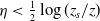 $\eta \lt \frac {1}{2}\log ({z_s}/{z})$
.
$\eta \lt \frac {1}{2}\log ({z_s}/{z})$
.
As before, the operator $L$
is in general not continuous on
$L$
is in general not continuous on $\mathcal{Z}$
; however, we give a dense subspace
$\mathcal{Z}$
; however, we give a dense subspace $\mathcal{Z}_{\mathcal{D}}$
of
$\mathcal{Z}_{\mathcal{D}}$
of $\mathcal{Z}$
in which it is bounded:
$\mathcal{Z}$
in which it is bounded:
Lemme 5.7.
Assume hypotheses (H1)–(H5). Then, there exists a constant $K\gt 0$
, depending only on
$K\gt 0$
, depending only on $(a_i)_{i\geq 1}$
,
$(a_i)_{i\geq 1}$
, $(b_i)_{i\geq 1}$
,
$(b_i)_{i\geq 1}$
, $z$
and
$z$
and $\eta$
, such that for all compactly supported sequence
$\eta$
, such that for all compactly supported sequence $h=(h_i)_{i\geq 1}$
, we have
$h=(h_i)_{i\geq 1}$
, we have
 \begin{equation*} \|L(h)\|_{\mathcal{Z}} \leq K\|h\|_{\mathcal{Z}_{\mathcal{D}}}. \end{equation*}
Proof. Using triangular inequality, it is sufficient to prove this bound separately for $S$
then
$S$
then $P$
. We already know from Cañizo and Lods [Reference Cañizo and Lods15, Lemma 3.3] that this is true for the operator
$P$
. We already know from Cañizo and Lods [Reference Cañizo and Lods15, Lemma 3.3] that this is true for the operator $S$
. We prove it for the operator
$S$
. We prove it for the operator $P$
. Recalling the definition of
$P$
. Recalling the definition of $P$
and using (H5), we have
$P$
and using (H5), we have
 \begin{align*} \|P(h)\|_{\mathcal{Z}} &\leq \exp\!(\eta )z\left (\frac {1}{z}\left (b_2\Theta _2|h_2| + \sum _{k=2}^{+\infty }b_k\Theta _k|h_k|\right )\right ) \\ &\leq 2b\exp\!(\eta )\sum _{k=1}^{+\infty }k^\eta \Theta _k|h_k|. \end{align*}
Then, using that $k^\beta \leq K(\eta ,\beta ) \exp\!(\eta k)$
for all
$k^\beta \leq K(\eta ,\beta ) \exp\!(\eta k)$
for all $k\geq 1$
and the positivity of
$k\geq 1$
and the positivity of $\sigma _k$
(5.19) for all
$\sigma _k$
(5.19) for all $k\geq 1$
, we have
$k\geq 1$
, we have
 \begin{align*} \|P(h)\|_{\mathcal{Z}} &\leq K(\eta ,\beta ) \sum _{k=1}^{+\infty }\exp\!(\eta k) \Theta _k|h_k| \\ &\leq K(\eta ,\beta ) \sum _{k=1}^{+\infty } (1+\sigma _k)\exp\!(\eta k) \Theta _k|h_k| = C\|h\|_{\mathcal{Z}_{\mathcal{D}}}. \end{align*}
Combining this estimation with the one on $S$
, we obtain the desired estimation.
$S$
, we obtain the desired estimation.
Following Cañizo and Lods [Reference Cañizo and Lods15], we extend the operator $L$
to an unbounded operator on
$L$
to an unbounded operator on $\mathcal{Z}$
that has a positive spectral gap using techniques based upon a suitable decomposition of the linearised operator into a dissipative part and a “regularising” part. To extend the operator, we use [Reference Cañizo and Lods15, Theorem 3.1], which is a slight improvement over some of the consequences of the work of Gualdani, Mischler and Mouhot [Reference Gualdani, Mischler and Mouhot30].
$\mathcal{Z}$
that has a positive spectral gap using techniques based upon a suitable decomposition of the linearised operator into a dissipative part and a “regularising” part. To extend the operator, we use [Reference Cañizo and Lods15, Theorem 3.1], which is a slight improvement over some of the consequences of the work of Gualdani, Mischler and Mouhot [Reference Gualdani, Mischler and Mouhot30].
Theorem 5.8 (Extension of the spectral gap). Assume hypotheses (H1)–(H5). Let $\eta \in (0,\frac {1}{2}\log (\frac {z_s}{z}))$
. If (
2.13
) is satisfied, then the extension of
$\eta \in (0,\frac {1}{2}\log (\frac {z_s}{z}))$
. If (
2.13
) is satisfied, then the extension of $L$
on
$L$
on $\mathcal{Z}_{\mathcal{D}}$
that we note
$\mathcal{Z}_{\mathcal{D}}$
that we note $\Lambda$
generates a strongly continuous semigroup
$\Lambda$
generates a strongly continuous semigroup $(\!\exp\!(t\Lambda ))_{t\geq 0}$
on
$(\!\exp\!(t\Lambda ))_{t\geq 0}$
on $\mathcal{Z}_{\mathcal{D}}$
and there exists
$\mathcal{Z}_{\mathcal{D}}$
and there exists $\mu _\ast \in (0,\mu _1]$
, a constant
$\mu _\ast \in (0,\mu _1]$
, a constant $K\gt 0$
such that
$K\gt 0$
such that
 \begin{equation} \|\exp\!(t\Lambda )x\|_{\mathcal{Z}} \leq K\exp\!(\!-\mu _\ast t)\|x\|_{\mathcal{Z}}, \,\forall t\geq 0 \text{ and } x\in \mathcal{Z}. \end{equation}
Proof. The proof follows the one of [Reference Cañizo and Lods15, Theorem 3.5]; to that end, we apply [Reference Cañizo and Lods15, Theorem 3.1]. The main modification is to add the operator $P$
in the regularising part of the decomposition of
$P$
in the regularising part of the decomposition of $\Lambda$
. We mean that an operator
$\Lambda$
. We mean that an operator $\mathcal{A}$
is regularising if for all
$\mathcal{A}$
is regularising if for all $h\in \mathcal{Z}$
,
$h\in \mathcal{Z}$
, $\mathcal{A}h \in \mathcal{H}$
. We just have to show that this is true for our operator
$\mathcal{A}h \in \mathcal{H}$
. We just have to show that this is true for our operator $P$
. Let
$P$
. Let $h\in \mathcal{Z}$
, we have
$h\in \mathcal{Z}$
, we have
 \begin{align*} \|P(h)\|_{\mathcal{H}}^2 &\leq \frac {4b^2}{z}\left (\sum _{k=1}^{+\infty }b_kQ_kz^kh_k\right )^2 \\ &\leq \frac {4b^2}{z}K(\beta ,\eta )\|h\|_{\mathcal{Z}}^2. \end{align*}
Then, the proof is straightforward following the proof of [Reference Cañizo and Lods15, Theorem 3.5]. We obtain that our operator has a spectral gap $\mu _\ast \in (0,\mu _1)$
.
$\mu _\ast \in (0,\mu _1)$
.
5.3.1. Proof of Theorem2.11
As stated before, we can obtain an estimation on the quadratic term in a weighted $\ell ^1$
space. Indeed, Cañizo and Lods [Reference Cañizo and Lods15, Proposition 3.2] proved an estimation on the quadratic term
$\ell ^1$
space. Indeed, Cañizo and Lods [Reference Cañizo and Lods15, Proposition 3.2] proved an estimation on the quadratic term $\Gamma$
, it reads as follows:
$\Gamma$
, it reads as follows:
Proposition 5.9.
Let $\eta \in (0,\frac {1}{2}\log (\frac {z_s}{z}))$
. There is a constant
$\eta \in (0,\frac {1}{2}\log (\frac {z_s}{z}))$
. There is a constant $K\gt 0$
, depending only on
$K\gt 0$
, depending only on $(a_i)_{i\geq 1}$
,
$(a_i)_{i\geq 1}$
, $(b_i)_{i\geq 1}$
, and
$(b_i)_{i\geq 1}$
, and $z$
, such that
$z$
, such that
 \begin{equation} \|\Gamma (h,h)\|_{\mathcal{Z}} \leq K\|h\|_{\mathcal{Z}}\|h\|_{\mathcal{Z}_{\mathcal{D}}},\,\forall h\in \mathcal{Z}_{\mathcal{D}}. \end{equation}
Let $\eta \in (0,\min \{\nu ,\frac {1}{2}\log \frac {z_s}{z}\})$
, where
$\eta \in (0,\min \{\nu ,\frac {1}{2}\log \frac {z_s}{z}\})$
, where $\nu$
comes from (2.7). The fluctuation
$\nu$
comes from (2.7). The fluctuation $h$
satisfies (5.16) in
$h$
satisfies (5.16) in $\mathcal{Z}$
, namely
$\mathcal{Z}$
, namely
 \begin{equation*} \frac {d}{dt}h = \Lambda h + \Gamma (h,h).\end{equation*}
Therefore, if $(V_t)_{t\geq 0}$
denotes the semigroup generates by
$(V_t)_{t\geq 0}$
denotes the semigroup generates by $\Lambda$
, we have
$\Lambda$
, we have
 \begin{equation*} h(t) = V_th(0) + \int _0^tV_{t-s}\Gamma (h(s),h(s))ds. \end{equation*}
Using Proposition5.9 and Theorem5.8, we have for some constant $C\gt 0$
,
$C\gt 0$
,
 \begin{align*} \|h(t)\|_{\mathcal{Z}} &\leq \|V_th(0)\|_{\mathcal{Z}} + \int _0^t\|V_{t-s}\Gamma (h(s),h(s))\|_{\mathcal{Z}} ds \\ &\leq K\|h(0)\|_{\mathcal{Z}}\exp\!(\!-\mu _\ast t) + K\exp\!(\!-\mu _\ast t)\int _0^t \exp\!(\mu _\ast s)\|\Gamma (h(s),h(s))\|_{\mathcal{Z}} ds \\ &\leq K\|h(0)\|_{\mathcal{Z}}\exp\!(\!-\mu _\ast t) + K\exp\!(\!-\mu _\ast t)\int _0^t \exp\!(\mu _\ast s)\|h(s)\|_{\mathcal{Z}}\|h(s)\|_{\mathcal{Z}_{\mathcal{D}}} ds, \end{align*}
For any $\upsilon \in (0,\nu -\eta )$
, using Cauchy–Schwarz’s inequality, we have
$\upsilon \in (0,\nu -\eta )$
, using Cauchy–Schwarz’s inequality, we have
 \begin{align*} \|h(t)\|_{\mathcal{Z}_{\mathcal{D}}} &= \sum _{i=1}^{+\infty } |h_i(t)|i\Theta _i\exp\!(\eta i) \\ &\leq \left (\sum _{i=1}^{+\infty } |h_i(t)|i\Theta _i\exp\!(\eta i-\upsilon i)\right )^{\frac {1}{2}}\left (\sum _{i=1}^{+\infty }|h_i(t)|i\Theta _i\exp\!(\eta i+\upsilon i)\right )^{\frac {1}{2}}. \end{align*}
However, $i\exp\!(\!-\upsilon i) \leq K$
, and
$i\exp\!(\!-\upsilon i) \leq K$
, and $i\exp\!(\eta i +\upsilon i) \leq K\exp\!(\nu i)$
, for all
$i\exp\!(\eta i +\upsilon i) \leq K\exp\!(\nu i)$
, for all $i\geq 1$
. Therefore, we deduce from (2.8) that
$i\geq 1$
. Therefore, we deduce from (2.8) that
 \begin{equation*}\|h(t)\|_{{\mathcal{Z}}_{\mathcal{D}}} \leq K \|h(t)\|_{\mathcal{Z}}^{\frac {1}{2}} \left (\sum _{i=1}^{+\infty }|h_i(t)|\Theta _i\exp\!(\nu i)\right )^{\frac {1}{2}} \leq K \Xi _1^\frac {1}{2}\|h(t)\|_{\mathcal{Z}}^{\frac {1}{2}}, \,\forall t\geq 0.\end{equation*}
All-in-one, we have
 \begin{equation*} \|h(t)\|_{\mathcal{Z}} \leq K\|h(0)\|_X\exp\!(\!-\mu _\ast t) + K\exp\!(\!-\mu _\ast t)\int _0^t \exp\!(\mu _\ast s)\|h(s)\|_{\mathcal{Z}}^\frac {3}{2} ds. \end{equation*}
Let $u(t) = \|h(t)\|_{\mathcal{Z}}\exp\!(\mu _\ast t)$
, we have
$u(t) = \|h(t)\|_{\mathcal{Z}}\exp\!(\mu _\ast t)$
, we have
 \begin{align*} u(t) &\leq K\|h(0)\|_{\mathcal{Z}} + K\int _0^t u(s)\|h(s)\|_{\mathcal{Z}}^{\frac {1}{2}} ds \\ &\leq K\varepsilon + K\int _0^t \exp \left (-\frac {\mu _\ast }{2}s\right )u(s)^{\frac {3}{2}} ds. \end{align*}
Using Grönwall’s lemma, we have for some $K\gt 0$
and
$K\gt 0$
and $\varepsilon$
small enough,
$\varepsilon$
small enough,
 \begin{equation*} u(t) \leq K. \end{equation*}
This means that
 \begin{equation*} \|h(t)\|_{\mathcal{Z}} \leq K\exp\!(\!-\mu _\ast t), \,\forall t\geq 0, \end{equation*}
which is exactly what we want. Indeed, recalling the ansatz $C_i = \Theta _i(1+h_i)$
, we have
$C_i = \Theta _i(1+h_i)$
, we have
 \begin{equation*} \|h(t)\|_{\mathcal{Z}} = \sum _{i=1}^{+\infty } e^{\eta i}Q_iz^i|h_i(t)| = \sum _{i=1}^{+\infty }e^{\eta i}|C_i(t)-Q_iz^i|, \end{equation*}
and therefore, the previous inequality is exactly (2.15).
6. Numerical simulations
6.1. Numerical scheme
In this section, we describe a numerical scheme used for the conservative truncation (2.16). At the end, we will make a few comments about the non-conservative truncation.
Let $n\geq 2$
be an integer. Recalling the PDE (2.17) and (2.18), it remains to add the boundary conditions. As we are considering the conservative truncation, we have on the right side of our domain the following boundary condition:
$n\geq 2$
be an integer. Recalling the PDE (2.17) and (2.18), it remains to add the boundary conditions. As we are considering the conservative truncation, we have on the right side of our domain the following boundary condition:
 \begin{equation} J(t,n) = 0. \end{equation}
Now, on the left side of our domain, which is the production of monomers, we have the following ODE:
 \begin{equation} \frac {d}{dt}C(t,1) = \lambda - \int _1^n a(x)C(t,1)C(t,x)dx - a(1)C(t,1)^2. \end{equation}
6.1.1. Verification of the choice of PDE
We verify that with the right discretisation and the right mesh, we retrieve our system of equations (2.16). To do this, we use a uniform mesh with a size step $\Delta x = 1$
, giving
$\Delta x = 1$
, giving
 \begin{equation*} C_i(t) \approx C(t,i), \,i=1,\ldots ,n. \end{equation*}
We discretise (2.17) using centre differences
 \begin{align*} \frac {\partial J(t,x)}{\partial x}\bigg |_{x=x_i} &\approx \frac {J(t,x_{i+1/2})-J(t,x_{i-1/2})}{\Delta x},\\ \frac {\partial }{\partial x}\left (\frac {C(t,x)}{Q(x)C(t,1)^x}\right )\bigg |_{x=x_{i+1/2}} &\approx \frac {1}{\Delta x}\left ( \frac {C_{i+1}(t)}{Q_{i+1}C_1^{i+1}(t)} - \frac {C_i(t)}{Q_iC_1^i(t)}\right )\!. \end{align*}
Therefore, since $\Delta x = 1$
and from (2.19), we obtain
$\Delta x = 1$
and from (2.19), we obtain
 \begin{equation*} \frac {\partial C(t,x)}{\partial t}\bigg |_{x=i} = -\frac {\partial J(t,x)}{\partial x}\bigg |_{x=i} \approx \frac {J_{i-1}(t)-J_i(t)}{\Delta x} = \frac {d}{dt}C_i(t). \end{equation*}
We just need to check the case $i=1$
, which comes from the left boundary condition (6.2). Using the rectangle rule to approximate the integral, we have
$i=1$
, which comes from the left boundary condition (6.2). Using the rectangle rule to approximate the integral, we have
 \begin{equation*} \frac {d}{dt}C(t,1) = \lambda - \int _1^n a(x)C(t,1)C(t,x) dx - a(1)C(t,1)^2 \approx \lambda - \sum _{j=1}^{n-1} a_jC_1(t)C_j(t) - a_1C_1(t)^2 = \frac {d}{dt}C_1(t). \end{equation*}
We have indeed found back our ODE (2.16) with a given scheme and a given mesh.
6.1.2. Reaction-diffusion (RD) scheme
We now follow the idea in [Reference Goudon and Monasse29] on a non-uniform mesh. Let $K\gt 0$
and
$K\gt 0$
and $\mathbb L$
the set of all the nodes in our non-uniform mesh:
$\mathbb L$
the set of all the nodes in our non-uniform mesh:
 \begin{equation*} \mathbb{L} = \left \{ n_1,\ldots ,n_K \,:\, n_j\lt n_{j+1},\, n_1=1,\,n_K=n \right \}\!. \end{equation*}
We then define the following size step:
 \begin{equation*} \Delta x_{j+1/2} = n_{j+1} - n_j \text{ and } \Delta x_j = n_{j+1/2}-n_{j-1/2} \text{ where } n_{j+1/2} = \frac {n_{j+1}+n_j}{2} \text{ with }n_j,n_{j+1}\in \mathbb{L}. \end{equation*}
Using finite volume scheme, we discretise (2.17) and (2.18) as follows:
 \begin{equation} C_{n_j}^{k+1}-C_{n_j}^k = \frac {\Delta t}{\Delta x_j}\left (J_{n_{j-1/2}}^{k+1}-J_{n_{j+1/2}}^{k+1}\right )\!, \end{equation}
with
 \begin{equation} J_{n_{j-1/2}}^{k+1} = -a_{n_{j-1/2}}Q_{n_{j-1/2}}\big(C_1^k\big)^{n_{j-1/2}+1/2}\frac {1}{\Delta x_{j-1/2}}\left (\frac {C_{n_j}^{k+1}}{Q_{n_j}\big(C_1^k\big)^{n_j}}-\frac {C_{n_{j-1}}^{k+1}}{Q_{n_{j-1}}\big(C_1^k\big)^{n_{j-1}}}\right )\!. \end{equation}
At this point, it remains to choose what is $a_{n_{j-1/2}}$
and
$a_{n_{j-1/2}}$
and $Q_{n_{j-1/2}}$
. To remain consistent with the discrete equations (i.e. when we take the step size equal to 1), we impose
$Q_{n_{j-1/2}}$
. To remain consistent with the discrete equations (i.e. when we take the step size equal to 1), we impose $a_{n_{j-1/2}} = a_{n_{j-1}}$
et
$a_{n_{j-1/2}} = a_{n_{j-1}}$
et $Q_{n_{j-1/2}} = Q_{n_{j-1}}$
. We have tried to impose something else, and the numerical results were not satisfying. Let
$Q_{n_{j-1/2}} = Q_{n_{j-1}}$
. We have tried to impose something else, and the numerical results were not satisfying. Let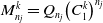 $M_{n_j}^k = Q_{n_j}\big(C_1^k\big)^{n_j}$
, we have
$M_{n_j}^k = Q_{n_j}\big(C_1^k\big)^{n_j}$
, we have
 \begin{equation*} Q_{n_{j-1}}\big(C_1^k\big)^{n_{j-1}} = M_{n_{j-1}} = \sqrt {M_{n_{j-1}}M_{n_j}}\sqrt {\frac {M_{n_{j-1}}}{M_{n_j}}} = \sqrt {M_{n_{j-1}}M_{n_j}}\sqrt {\prod _{k=n_{j-1}+1}^{n_j}\frac {b_k}{a_{k-1}}}\left (\sqrt {C_1^k}\right )^{-(n_j-n_{j-1})}. \end{equation*}
Using the above equality, we can rewrite (6.3), we obtain for all $2\leq j\leq K-1$
,
$2\leq j\leq K-1$
,
 \begin{align*} C_{n_j}^{k+1}-C_{n_j}^k &= \frac {\Delta t}{\Delta x_j}\sqrt {M_j^k}\left (\frac {a_{n_j}\sqrt {C_1^k}}{\Delta x_{j+1/2}}\sqrt {\prod _{k=n_{j}+1}^{n_{j+1}}\frac {b_k}{a_{k-1}}}\frac {C_{n_{j+1}}^{k+1}}{\sqrt {M_{n_j}^k}} + \frac {a_{n_{j-1}}\sqrt {C_1^k}}{\Delta x_{j-1/2}} \sqrt {\prod _{k=n_{j-1}+1}^{n_j}\frac {b_k}{a_{k-1}}} \frac {C_{n_{j-1}}^k}{\sqrt {M_{n_{j-1}}^k}} \right . \\ & \quad \left . - \left ( \frac {a_{n_j}}{\Delta x_{j+1/2}}\left (\sqrt {C_1^k}\right )^{n_{j+1}-n_j+1} + \frac {a_{n_{j-1}}}{\Delta x_{j-1/2}} \left [ \prod _{k=n_{j-1}+1}^{n_j}\frac {b_k}{a_{k-1}}\right ]\left (\sqrt {C_1^k}\right )^{1-(n_j-n_{j-1})} \right ) \frac {C_{n_j}^{k+1}}{\sqrt {M_{n_j}^k}} \right )\!. \end{align*}
Let $h_{n_j}^\ast \,:\!=\, \dfrac {C_{n_j}^{k+1}}{\sqrt {M_{n_j}^k}}$
and
$h_{n_j}^\ast \,:\!=\, \dfrac {C_{n_j}^{k+1}}{\sqrt {M_{n_j}^k}}$
and $h_{n_j} = \dfrac {C_{n_j}^k}{\sqrt {M_{n_j}^k}}$
, we then have for all
$h_{n_j} = \dfrac {C_{n_j}^k}{\sqrt {M_{n_j}^k}}$
, we then have for all $2\leq j \leq K-1$
,
$2\leq j \leq K-1$
,
 \begin{align*} h_{n_j}^{\ast } &= h_{n_j}^k + \frac {\Delta t}{\Delta x_j}\left (\frac {a_{n_j}}{\Delta x_{j+1/2}}\sqrt {\prod _{k=n_{j}+1}^{n_{j+1}}\frac {b_k}{a_{k-1}}}\sqrt {C_1^k}h_{n_{j+1}}^\ast + \frac {a_{n_{j-1}}}{\Delta x_{j-1/2}} \sqrt {\prod _{k=n_{j-1}+1}^{n_j}\frac {b_k}{a_{k-1}}} \sqrt {C_1^k} h_{n_{j-1}}^\ast \right . \\ &\quad \left . - \left ( \frac {a_{n_j}}{\Delta x_{j+1/2}}\left (\sqrt {C_1^k}\right )^{n_{j+1}-n_j+1} + \frac {a_{n_{j-1}}}{\Delta x_{j-1/2}} \left [ \prod _{k=n_{j-1}+1}^{n_j}\frac {b_k}{a_{k-1}}\right ]\left (\sqrt {C_1^k}\right )^{1-(n_j-n_{j-1})}\right )h_{n_j}^\ast \right )\!. \end{align*}
As mentioned in the beginning of this section, we present this scheme on the conservative truncation (2.16); thus, we impose the zero flux condition on the right boundary, meaning $J_{n_{K+1/2}} = 0$
. This condition may be rewritten as follows:
$J_{n_{K+1/2}} = 0$
. This condition may be rewritten as follows:
 \begin{equation} \frac {C_{n_{K+1}}^{k+1}}{M_{n_{K+1}}^k} = \frac {C_{n_K}^{k+1}}{M_{n_K}^k},\,\, \forall k\gt 0. \end{equation}
Therefore, the scheme becomes
 \begin{align} C_1^{k+1} &= C_1^k + \Delta t \left ( \lambda - C_1^{k+1}\left (\sum _{j=1}^{K-1} a_{n_j}\Delta x_{j+1/2}C_{n_j}^k+a_1C_1^k\right )\right ) \nonumber\\ h_1^\ast &= \frac {1}{\sqrt {C_1^k}} \frac {C_1^k + \lambda \Delta t}{1+\Delta t\left (\sum \limits _{j=1}^{K-1} a_{n_j}\Delta x_{j+1/2}C_{n_j}^k+a_1C_1^k\right )} \nonumber\\ h_{n_j}^{\ast } &= h_{n_j}^k + \frac {\Delta t}{\Delta x_j}\left (\frac {a_{n_j}}{\Delta x_{j+1/2}}\sqrt {\prod _{k=n_{j}+1}^{n_{j+1}}\frac {b_k}{a_{k-1}}}\sqrt {C_1^k}h_{n_{j+1}}^\ast + \frac {a_{n_{j-1}}}{\Delta x_{j-1/2}} \sqrt {\prod _{k=n_{j-1}+1}^{n_j}\frac {b_k}{a_{k-1}}} \sqrt {C_1^k} h_{n_{j-1}}^\ast \right . \nonumber\\ & \quad \left . - \left ( \frac {a_{n_j}}{\Delta x_{j+1/2}}\left (\sqrt {C_1^k}\right )^{n_{j+1}-n_j+1} + \frac {a_{n_{j-1}}}{\Delta x_{j-1/2}} \left [ \prod _{k=n_{j-1}+1}^{n_j}\frac {b_k}{a_{k-1}}\right ]\left (\sqrt {C_1^k}\right )^{1-(n_j-n_{j-1})}\right )h_{n_j}^\ast \right ) \nonumber\\ h_{n_K}^\ast &= h_{n_K} + \frac {\Delta t}{\Delta x_K}\left ( \frac {a_{n_{K-1}}}{\Delta x_{K-1/2}}\sqrt {\prod _{k=n_{K-1}+1}^{n_K} \frac {b_k}{a_{k-1}}}\sqrt {C_1^k}h_{n_{K-1}} \right . \nonumber\\ & \qquad\qquad\qquad \left . - \frac {a_{n_{K-1}}}{\Delta x_{K-1/2}}\left [\prod _{k=n_{K-1}+1}^{n_K} \frac {b_k}{a_{k-1}} \right ] \left (\sqrt {C_1^k}\right )^{1-(n_K-n_{K-1})}h_{n_K} \right )\!. \end{align}
Numerically to implement (6.6), we solve the following linear system:
 \begin{equation} \left (I_{K-1} - \Delta t\mathsf{W}^k\right )H^\ast = H + \beta ^k, \end{equation}
where
 \begin{equation*} H^\ast = \begin{pmatrix} h_2^\ast \\ \vdots \\ \vdots \\ \vdots \\ h_{n_K}^\ast \end{pmatrix}, \,\, H = \begin{pmatrix} h_2 \\ \vdots \\ \vdots \\ \vdots \\ h_{n_K} \end{pmatrix}, \,\, \beta ^k = \frac {\Delta t}{\Delta x_2 \Delta x_{2-1/2}}a_{n_1}\sqrt {C_1^k}\sqrt {\prod _{k=n_1+1}^{n_2}\frac {b_k}{a_{k-1}}} \begin{pmatrix} h_1^\ast \\ 0 \\ \vdots \\ \vdots \\ \vdots \\ 0 \end{pmatrix}, \end{equation*}
and the tri-diagonal matrix
with for $2\leq j\leq K-1$
,
$2\leq j\leq K-1$
,
 \begin{equation*} \omega _{n_j}^k = \frac {1}{\Delta x_j}\left (\frac {a_{n_{j}}}{\Delta x_{j+1/2}}\left (\sqrt {C_1^k}\right )^{n_{j+1}-n_j+1} + \frac {a_{n_{j-1}}}{\Delta x_{j-1/2}} \left [ \prod _{k=n_{j-1}+1}^{n_j}\frac {b_k}{a_{k-1}}\right ]\left (\sqrt {C_1^k}\right )^{1-(n_j-n_{j-1})} \right )\!, \end{equation*}
 \begin{equation*} \alpha _{n_{j+1/2}} = \frac {1}{\Delta x_j}\frac {a_{n_j}}{\Delta x_{j+1/2}}\sqrt {\prod _{k=n_{j}+1}^{n_{j+1}}\frac {b_k}{a_{k-1}}}\sqrt {C_1^k}, \,\, \gamma _{n_{j-1/2}} = \frac {1}{\Delta x_{j}}\frac {a_{n_{j-1}}}{\Delta x_{j-1/2}} \sqrt {\prod _{k=n_{j-1}+1}^{n_j}\frac {b_k}{a_{k-1}}} \sqrt {C_1^k}, \end{equation*}
and
 \begin{equation*} \nu _{n_K}^k = \frac {1}{\Delta x_K}\frac {a_{n_{K-1}}}{\Delta x_{K-1/2}}\left [\prod _{k=n_{K-1}+1}^{n_K} \frac {b_k}{a_{k-1}} \right ] \left (\sqrt {C_1^k}\right )^{1-(n_K-n_{K-1})}. \end{equation*}
Remark 6.1.
As opposed to uniform mesh, the matrix $\mathsf{W}^k$
is no longer symmetric, which can translate in a loss of computation time. Therefore, to symmetrise this matrix while keeping the tri-diagonal form, we can multiply the matrix by
$\mathsf{W}^k$
is no longer symmetric, which can translate in a loss of computation time. Therefore, to symmetrise this matrix while keeping the tri-diagonal form, we can multiply the matrix by
 \begin{equation*} \mathsf{\Theta } = \text{diag}\left (\frac {\Delta x_j}{\Delta x_1}\right )_{2\leq j\leq K}. \end{equation*}
The scheme on $h^\ast$
(6.6) is unconditionally stable in time and size. Indeed, the only restriction could be on the time step because of Euler’s explicit–implicit scheme for
$h^\ast$
(6.6) is unconditionally stable in time and size. Indeed, the only restriction could be on the time step because of Euler’s explicit–implicit scheme for $C_1$
, but this scheme is also unconditionally stable. We have
$C_1$
, but this scheme is also unconditionally stable. We have
 \begin{equation*} C_1^{k+1}\left (1+\Delta t\left (a_1C_1^k+\sum _{j=1}^{K-1}a_{n_j}\Delta x_{j+1/2}C_{n_j}^k\right )\right ) = C_1^k + \Delta t \lambda \end{equation*}
thus
 \begin{equation*} C_1^{k+1} \leq C_1^k + \Delta t \lambda , \end{equation*}
which leads to, for $0\leq t^k \leq T$
,
$0\leq t^k \leq T$
,
 \begin{equation*} C_1^{k} \leq C_1^0 + \lambda t^k \leq C_1^0 + \lambda T. \end{equation*}
Remark 6.2.
We could just do an Euler explicit scheme for (
6.2
), but then we would have two conditions on the time step $\Delta t$
: stability and to preserve positivity. This would lead to having an adaptive time step
$\Delta t$
: stability and to preserve positivity. This would lead to having an adaptive time step $\Delta t^k$
.
$\Delta t^k$
.
We now have a well-balanced scheme that is unconditionally stable in time and size. However, there is a difference with the uniform mesh with $\Delta x = 1$
or with the ODEs, which is the parameter
$\Delta x = 1$
or with the ODEs, which is the parameter $z$
of the steady-state. Indeed, equation (6.6) for
$z$
of the steady-state. Indeed, equation (6.6) for $j\geq 2$
implies that the steady state is of the form
$j\geq 2$
implies that the steady state is of the form $Q_{n_j}\eta ^{n_j}$
, and the parameter
$Q_{n_j}\eta ^{n_j}$
, and the parameter $\eta$
is determined with the equation on
$\eta$
is determined with the equation on $C_1$
. The difference comes from the following two equations:
$C_1$
. The difference comes from the following two equations:
 \begin{equation} \lambda - \sum _{i=1}^{N-1} a_iQ_iz^{i+1} - a_1z^2 = 0 \text{ and } \lambda - \sum _{j=1}^{K-1} a_{n_j}\Delta x_{n_{j+1/2}}Q_{n_j}\tilde z^{n_j+1} - a_{n_1}\tilde z^2 = 0, \end{equation}
which do not have the same solutions. In fact, the difference of the two solutions is of order $Q_{n_l}\tilde z^{n_l}$
where
$Q_{n_l}\tilde z^{n_l}$
where $l$
is defined as follows:
$l$
is defined as follows:
 \begin{equation*} l = \min \left \{ j \in \left \{1,\ldots ,K-1\right \} \,:\, \Delta x_{j+1/2} \gt 1 \right \}\!. \end{equation*}
A difference is expected since we reduce the linear system; therefore, we lost information that translates into a slight difference in the steady state. We note that we can compute the steady state on a uniform mesh with $\Delta x = 1$
and, therefore, choose the right mesh to control the error. Morally, if we choose a mesh with
$\Delta x = 1$
and, therefore, choose the right mesh to control the error. Morally, if we choose a mesh with $\Delta x = 1$
for small size and whatever we want for bigger size, then we approach the right steady state.
$\Delta x = 1$
for small size and whatever we want for bigger size, then we approach the right steady state.
Remark 6.3 (Non-conservative truncation). Changing the right boundary condition ( 6.5 ) to one taking account things that can leave the system, we obtain the same scheme except for the bottom right term in the iteration matrix. However, the scheme is no longer well-balanced since we still use the same form of steady state. One modification could be to use the steady state of the non-conservative truncation and doing again the same scheme.
6.2. Numerical results
Before showing numerical results, we have to mention the fact that the conservative truncation (2.16) has the same steady state as the infinite system, meaning $(Q_iz^i)_{i\geq 1}$
; however, the
$(Q_iz^i)_{i\geq 1}$
; however, the $z$
differs due to the truncation. In fact, the conservative truncation (2.16) has a unique steady state, which is this one, no matter
$z$
differs due to the truncation. In fact, the conservative truncation (2.16) has a unique steady state, which is this one, no matter $\lambda$
. There is no sub-critical or super-critical cases in any truncation; indeed, if
$\lambda$
. There is no sub-critical or super-critical cases in any truncation; indeed, if $z_s$
is finite, then for a fixed
$z_s$
is finite, then for a fixed $n$
and
$n$
and $\lambda$
there always exists
$\lambda$
there always exists $z(n)\gt z_s$
such that
$z(n)\gt z_s$
such that $(Q_iz(n)^i)_{1\leq i\leq n}$
is the only steady state of (2.16).
$(Q_iz(n)^i)_{1\leq i\leq n}$
is the only steady state of (2.16).
Following the above discussion on $z$
for different meshes, we denote
$z$
for different meshes, we denote $z_{RK4} = z_{RDU}$
the parameter
$z_{RK4} = z_{RDU}$
the parameter $z$
obtained with the full sum, meaning with
$z$
obtained with the full sum, meaning with $\Delta x = 1$
, and we denote
$\Delta x = 1$
, and we denote $z_{RDNU}$
the parameter
$z_{RDNU}$
the parameter $z$
obtained with a non-uniform mesh. Consequently, we denote
$z$
obtained with a non-uniform mesh. Consequently, we denote $C^{eq}_{RK4} = C^{eq}_{RDU}$
and
$C^{eq}_{RK4} = C^{eq}_{RDU}$
and $C^{eq}_{RDNU}$
the corresponding steady state.
$C^{eq}_{RDNU}$
the corresponding steady state.
In every numerical simulation used to obtain graphs below, we start with a system containing nothing:
 \begin{equation*} C_i(0) = 0, \,\text{for } i = 1,\ldots ,n. \end{equation*}
For the size discretisation, we use a non-uniform mesh with $\Delta x = 1$
close to the boundaries and then nodes are spaced evenly on a log scale until the step size reaches the maximum size that we impose.
$\Delta x = 1$
close to the boundaries and then nodes are spaced evenly on a log scale until the step size reaches the maximum size that we impose.
We start with the convergence towards the steady state of our numerical solution. Figure 1 shows results for a system of size $n = 30 000$
with kinetics coefficients and production rate as follows:
$n = 30 000$
with kinetics coefficients and production rate as follows:
 \begin{equation} a_i = i^{1/2}, \,b_i = i^{2/3} \text{ and } \lambda = 10. \end{equation}
These parameters give $z_s = +\infty$
, and therefore,
$z_s = +\infty$
, and therefore, $\lambda _s = +\infty$
and z
$\lambda _s = +\infty$
and z $\approx$
1.119. Using our coarse-grain mesh, we have
$\approx$
1.119. Using our coarse-grain mesh, we have $|\texttt {z}_{RDU}-\texttt {z}_{RDNU}| \leq \texttt {1.8e-8}$
.
$|\texttt {z}_{RDU}-\texttt {z}_{RDNU}| \leq \texttt {1.8e-8}$
.
Figure 1a shows that the numerical solution of our scheme converges towards the steady-state $(Q_iz_{RDNU}^i)_{1\leq i\leq n}$
at the given precision, and the green curve shows what we expected, which is that the two equilibria differ at the expected order of magnitude. Focusing on the red and blue curves, our scheme preserves the exponential decay towards the steady state. Figure 1b shows that the relative error between the numerical solution obtained from our scheme and the one obtained with RK4 scheme (Runge–Kutta method) converges towards the relative error between the different equilibria, which is expected from Figure 1b and (6.8). However, unlike the scheme of Duncan and Soheili [Reference Duncan and Soheili26, Figure 3], the relative error does not behave similarly. Indeed, their relative error is close to 0 for small time but remains around
$(Q_iz_{RDNU}^i)_{1\leq i\leq n}$
at the given precision, and the green curve shows what we expected, which is that the two equilibria differ at the expected order of magnitude. Focusing on the red and blue curves, our scheme preserves the exponential decay towards the steady state. Figure 1b shows that the relative error between the numerical solution obtained from our scheme and the one obtained with RK4 scheme (Runge–Kutta method) converges towards the relative error between the different equilibria, which is expected from Figure 1b and (6.8). However, unlike the scheme of Duncan and Soheili [Reference Duncan and Soheili26, Figure 3], the relative error does not behave similarly. Indeed, their relative error is close to 0 for small time but remains around $10^{-2}$
when the solution reaches the steady state, whereas our relative error is bigger for small time but decreases towards the expected error (the sub-sampling error from (6.8)) as the solution reaches the steady state.
$10^{-2}$
when the solution reaches the steady state, whereas our relative error is bigger for small time but decreases towards the expected error (the sub-sampling error from (6.8)) as the solution reaches the steady state.
Comparison of the convergence towards the steady state. System size $K = 649$
with maximum step size
$K = 649$
with maximum step size $\Delta x_{max} = 50$
. The relative error is only taken from the nodes on the non-uniform mesh, no interpolation is used.
$\Delta x_{max} = 50$
. The relative error is only taken from the nodes on the non-uniform mesh, no interpolation is used.

We now compare computation time, since for the super-critical case, we may need to compute very large size for a very long time. We, therefore, want a scheme that is able to reduce the computation time. In our scheme, we take $\Delta x_{max}$
such that it represents at most 0.05% of the truncation size
$\Delta x_{max}$
such that it represents at most 0.05% of the truncation size $n$
. Figure 2 shows that, for large enough truncation size
$n$
. Figure 2 shows that, for large enough truncation size $n$
, it is efficient to use our scheme.
$n$
, it is efficient to use our scheme.
Figure 2a shows results with kinetics coefficients and production rate from (6.9), and Figure 2b shows results with kinetics coefficients and production rate as follows:
 \begin{equation} a_i = i^{1/2}, \,b_i = 0.1+0.75i^{1/2} \text{ and } \lambda = 1. \end{equation}
These parameters give $z_s = 0.75$
,
$z_s = 0.75$
, $\lambda _s$ $\approx$
5.34375 and z
$\approx$
5.34375 and z $\approx$
0.516.
$\approx$
0.516.
We mention that with other coefficients (e.g. (6.11)), the convergence is much slower towards the steady-state and therefore the gain can be much better. Taking the maximum size $n=30000$
and allowing only
$n=30000$
and allowing only $\Delta x_{max}$
to be roughly
$\Delta x_{max}$
to be roughly $0.05\%$
of
$0.05\%$
of $n$
, we reduce the computational time by
$n$
, we reduce the computational time by $65\%$
. Taking
$65\%$
. Taking $\Delta x_{max}$
to be roughly
$\Delta x_{max}$
to be roughly $0.5\%$
of
$0.5\%$
of $n$
, the reduction becomes
$n$
, the reduction becomes $80\%$
. The gain of computational time also comes from the time size, which is
$80\%$
. The gain of computational time also comes from the time size, which is $10$
times bigger for our scheme.
$10$
times bigger for our scheme.
 \begin{equation} a_i = i^{1/2}, \,b_i = 0.05+0.1i^{2/3} \text{ and } \lambda = 10. \end{equation}
Comparison of computation time.

We now compare the dynamics of our numerical solution. We know that the convergence towards the steady state is the same and that for large truncation it is more efficient time wise. However, is the behaviour, quantitatively and qualitatively speaking, of our solution the same or not? Figure 3 shows that it globally conserves the dynamical behaviour of the solution with the same order of magnitude. We only show the first coordinate since the dynamical behaviour is led by the latter. We note that in those simulations, neither $\Delta t$
nor
$\Delta t$
nor $\Delta x_j$
is the same as in the RK4 scheme, which already creates an error.
$\Delta x_j$
is the same as in the RK4 scheme, which already creates an error.
Figure 3 shows results with kinetics coefficients and production rate from (6.9).
One more reason we want to develop a different scheme and not settle for classical ODE schemes is for the super-critical case. Indeed, as stated before, either truncation have a unique steady state, but they are not necessarily the one (or ones) of the infinite system, and moreover, they do not necessarily converge as $n$
goes to infinity to the one (or ones) of the infinite system. In practice, we observe that the numerical solution of the RK4 scheme (Runge–Kutta method) always converges towards the steady state of the truncation even in the theoretical super-critical case.
$n$
goes to infinity to the one (or ones) of the infinite system. In practice, we observe that the numerical solution of the RK4 scheme (Runge–Kutta method) always converges towards the steady state of the truncation even in the theoretical super-critical case.
Comparison of the dynamical behaviour of $C_1(t)$
.
$C_1(t)$
.

We might expect a different behaviour of our scheme, leading to hints of what is happening in the super-critical case. There is no steady state, but as in the Becker–Döring equations, it still could converge towards $(Q_iz_s^i)_{i\geq 1}$
in some sense, even if it is not a steady state, unlike in the Becker–Döring equations. We then believe that our scheme may be able to catch a very slow convergence towards this sequence that a classical numerical scheme on the truncation system would definitely not catch.
$(Q_iz_s^i)_{i\geq 1}$
in some sense, even if it is not a steady state, unlike in the Becker–Döring equations. We then believe that our scheme may be able to catch a very slow convergence towards this sequence that a classical numerical scheme on the truncation system would definitely not catch.
Acknowledgements
The author would like to thank Erwan Hingant for many valuable discussions on the topics covered in this paper.
Competing interests
The author declares none.
Appendix A. Estimations of the sufficient condition
A.1. Constant coefficients
We detail the computation to obtain Example2.13. Recalling that $a_i=a$
and
$a_i=a$
and $b_i=b$
for all
$b_i=b$
for all $i\geq 1$
, we have for
$i\geq 1$
, we have for $z\lt z_s$
,
$z\lt z_s$
, $\frac {b}{a}=z_s$
and
$\frac {b}{a}=z_s$
and
 \begin{align*} Q_i = \prod _{j=2}^{i}\frac {a_{j-1}}{b_j}=\prod _{j=2}^{i}\frac {a}{b} = \left (\frac {a}{b}\right )^{i-1} = \frac {1}{z_s^{i-1}}. \end{align*}
Thus,
 \begin{align*} \sum _{k=1}^{+\infty } Q_kz^k = z_s\sum _{k=1}^{+\infty } \left (\frac {z}{z_s}\right )^k = \frac {zz_s}{z_s-z}, \end{align*}
and
 \begin{align*} \sum _{j=1}^k \frac {1}{a_jQ_jz^j} = \frac {1}{a} \sum _{j=1}^k \frac {z_s^{j-1}}{z^j} = \frac {1}{az_s}\frac {\frac {z}{z_s}-\left (\frac {z_s}{z}\right )^{k+1}}{1-\frac {z}{z_s}} = \frac {1}{a}\frac {1-\left (\frac {z_s}{z}\right )^k}{z-z_s}, \end{align*}
and
 \begin{align*} \sum _{j=k+1}^{+\infty }Q_jz^j = z_s\sum _{j=k+1}^{+\infty }\left (\frac {z}{z_s}\right )^j = \frac {z}{1-\frac {z}{z_s}}-\frac {z-z_s\left (\frac {z}{z_s}\right )^{k+1}}{1-\frac {z}{z_s}} = \frac {z_s^2}{z_s-z}\left (\frac {z}{z_s}\right )^{k+1}. \end{align*}
We then obtain
 \begin{align*} \left (\sum _{j=k+1}^{+\infty }Q_jz^j\right )\left (\sum _{j=1}^k \frac {1}{a_jQ_jz^j}\right ) = -\frac {1}{a}\frac {z_s^2}{(z_s-z)^2}\left (\frac {z}{z_s}\right )^{k+1} + \frac {1}{a}\frac {zz_s}{(z_s-z)^2}. \end{align*}
Therefore, the condition (2.13) becomes
 \begin{align*} \frac {8b}{\sqrt {z}}\sqrt {\frac {zz_s}{z_s-z}} \frac {1}{a}\frac {zz_s}{(z_s-z)^2} \lt 1, \end{align*}
which is, after simplification,
 \begin{align*} \frac {8zz_s^{5/2}}{(z_s-z)^{5/2}}\lt 1. \end{align*}
A.2. Linear coefficients
We detail the computation to obtain the Example2.14. Recalling that $a_i=ai$
and
$a_i=ai$
and $b_i=bi$
for all
$b_i=bi$
for all $i\geq 1$
, we have for
$i\geq 1$
, we have for $z\lt z_s$
,
$z\lt z_s$
, $\frac {b}{a}=z_s$
and
$\frac {b}{a}=z_s$
and
 \begin{align*} Q_i = \prod _{j=2}^{i}\frac {a_{j-1}}{b_j}=\prod _{j=2}^{i}\frac {a(j-1)}{bj} = \left (\frac {a}{b}\right )^{i-1}\prod _{j=2}^{i}\frac {j-1}{j} = \left (\frac {a}{b}\right )^{i-1}\frac {1}{i} = \frac {1}{iz_s^{i-1}}. \end{align*}
Thus,
 \begin{align*} \sum _{i=1}^{+\infty }i^2Q_iz^i &= z\sum _{i=1}^{+\infty }i\left (\frac {z}{z_s}\right )^{i-1} = z\sum _{i=1}^{+\infty }\left [\left (\frac {z}{z_s}\right )^{i}\right ]^{\prime} \\ &= z\left [\sum _{i=1}^{+\infty }\left (\frac {z}{z_s}\right )^{i}\right ]^{\prime} = z\left (\frac {\frac {z}{z_s}}{1-\frac {z}{z_s}}\right )^{\prime} \\ &=\frac {zz_s}{(z_s-z)^2}, \end{align*}
and
 \begin{align*} \sum _{j=1}^k \frac {1}{a_jQ_jz^j} = \frac {1}{a} \sum _{j=1}^k \frac {z_s^{j-1}}{z^j} = \frac {1}{az_s}\frac {\frac {z}{z_s}-\left (\frac {z_s}{z}\right )^{k+1}}{1-\frac {z}{z_s}} = \frac {1}{a}\frac {1-\left (\frac {z_s}{z}\right )^k}{z-z_s}, \end{align*}
and
 \begin{align*} \sum _{j=k+1}^{+\infty }Q_jz^j &= \frac {b}{a}\sum _{j=k+1}^{+\infty }\frac {1}{j}\left (\frac {z}{z_s}\right )^j = z_s\sum _{j=k+1}^{+\infty }\int _0^z \left (\frac {x}{z_s}\right )^{j-1}dx \\ &= z_s \int _0^z \frac {\left (\frac {x}{z_s}\right )^k}{1-\frac {x}{z_s}}dx. \\ \end{align*}
Therefore, the condition (2.13) becomes
 \begin{equation*} \frac {8z_s^{3/2}}{z_s-z}\sup _{k\geq 1}\left (\int _0^z \frac {\left (\frac {x}{z_s}\right )^k}{1-\frac {x}{z_s}}dx\right )\left (\frac {1-\left (\frac {z_s}{z}\right )^k}{z-z_s}\right ) \lt 1. \end{equation*}
However, for $z\lt \dfrac {z_s}{2}$
(
$z\lt \dfrac {z_s}{2}$
( $z$
small enough), we have
$z$
small enough), we have $\dfrac {1}{z_s-z}\lt \dfrac {2}{z_s}$
. Thus, for
$\dfrac {1}{z_s-z}\lt \dfrac {2}{z_s}$
. Thus, for $k\geq 1$
,
$k\geq 1$
,
 \begin{align*} \left (\int _0^z \frac {\left (\frac {x}{z_s}\right )^k}{1-\frac {x}{z_s}}dx\right )\left (\frac {1-\left (\frac {z_s}{z}\right )^k}{z-z_s}\right ) &\lt \frac {4}{z_s^2}\int _0^z\left (\frac {x}{z_s}\right )^k\left [\left (\frac {z_s}{z}\right )^k-1\right ] \\ &\lt \frac {4}{z_s^2}\frac {z_s}{k+1}\left (\frac {z}{z_s}\right )^{k+1}\left [\left (\frac {z_s}{z}\right )^k-1\right ] \\ &\lt \frac {4}{z_s}\frac {1}{k+1}\frac {z}{z_s} \\ &\lt \frac {4z}{z_s^2}. \end{align*}
Therefore, the condition (2.13) is true when
 \begin{equation*} \frac {32z}{\sqrt {z_s}(z_s-z)}\lt 1. \end{equation*}


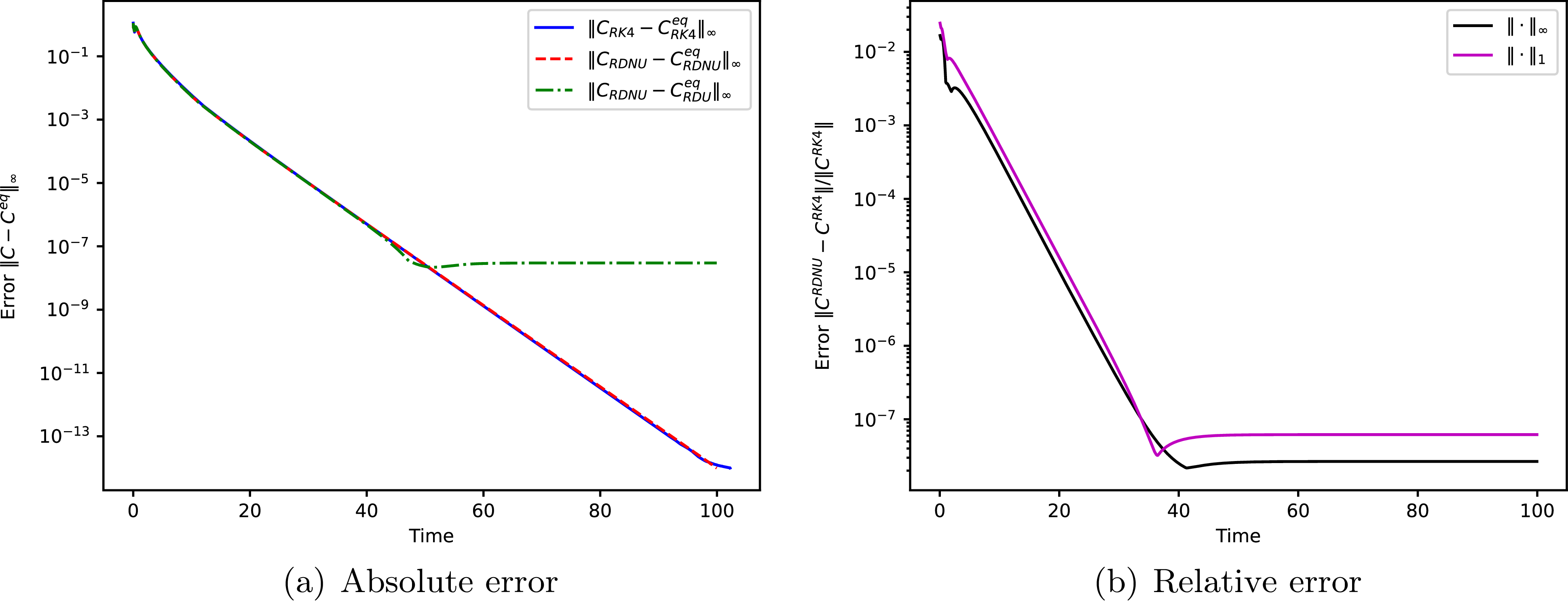


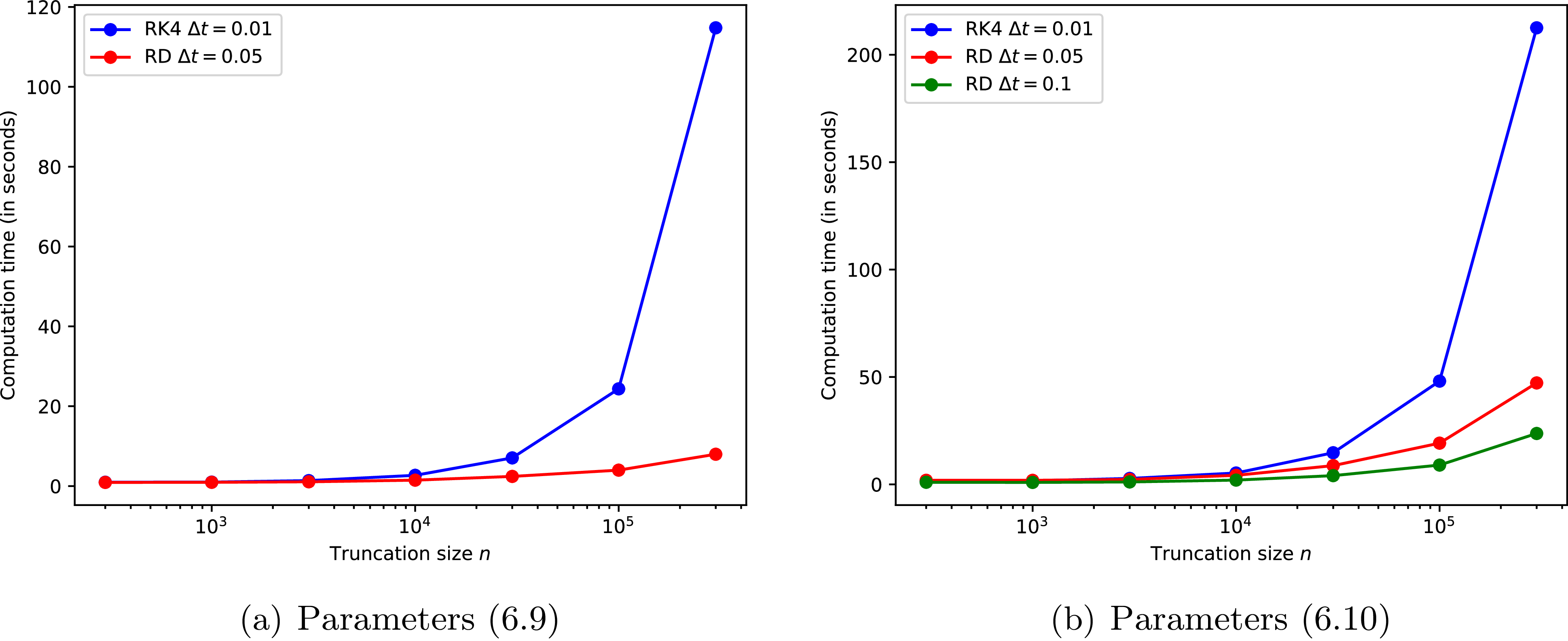
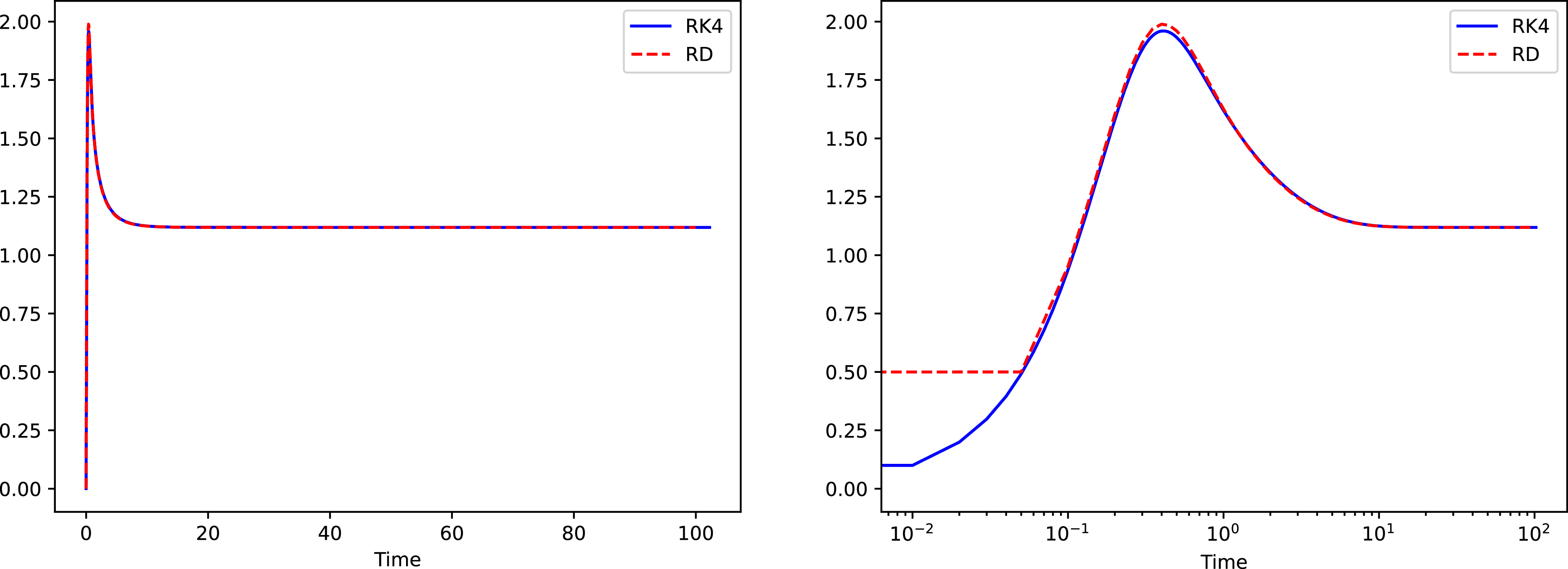


 Open access

