


1 Introduction
In recent years, large-scale educational assessments, such as the Programme for International Student Assessment (PISA; OECD, 2021), the National Assessment of Educational Progress (NAEP; Johnson & Jenkins, Reference Johnson and Jenkins2004), the Trends in International Mathematics and Science Study (TIMSS; Martin & Kelly, Reference Martin and Kelly1996), and the Progress in International Reading Literacy Study (PIRLS; Mullis et al., Reference Mullis, Martin and Gonzalez2003), have become central to global education research. These assessments produce large-scale and multifaceted datasets, providing valuable insights into student knowledge, skills, and learning behaviors. However, traditional large-scale educational data is typically static and updated periodically, making it challenging to capture the dynamic changes in educational environments and the real-time status of students’ learning. With advances in information technology, online testing platforms and educational assessment tools like adaptive testing now allow the collection of real-time data on students’ responses and behaviors, providing new possibilities for dynamically evaluating educational processes and learning outcomes. Real-time data are characterized by its high speed, large volume, and complexity, requiring efficient computational methods to quickly identify patterns, detect learning obstacles, and predict outcomes. In addition, leveraging this real-time data allows educators to adjust teaching strategies promptly and offer personalized learning experiences for students.
The increasing availability and complexity of large-scale educational datasets have highlighted the need for robust analytical frameworks to handle such data efficiently. Item response theory (IRT; van der Linden & Hambleton, Reference van der Linden and Hambleton1997) has emerged as a powerful tool for analyzing such large datasets. In IRT, parameter estimation is a core component that directly determines the model’s scientific validity and the interpretation of results. The most commonly used estimation method in IRT is marginal maximum likelihood estimation based on the expectation–maximization algorithm (MMLE-EM; Baker & Kim, Reference Baker and Kim2004; Bock & Aitkin, Reference Bock and Aitkin1981). MMLE-EM utilizes an iterative optimization approach that is highly efficient in managing missing data or complex item response datasets, making it particularly adaptable to large-scale educational assessments. However, the computational complexity of this method is primarily influenced by the dimensionality of the latent variables. As the dimensionality of the latent variables increases linearly, the number of quadrature nodes required for integration in the E-step grows exponentially, leading to a substantial increase in computational cost and difficulty.
To address these challenges, current research on IRT focuses on improving computational efficiency for high-dimensional numerical integration. Several methods have been proposed, including adaptive Gaussian quadrature EM algorithms (Rabe-Hesketh et al., Reference Rabe-Hesketh, Skrondal and Pickles2005; Schilling & Bock, Reference Schilling and Bock2005), Laplace approximation methods (Huber et al., Reference Huber, Ronchetti and Victoria-Feser2004; Thomas, Reference Thomas1993), Monte Carlo EM algorithms (Meng & Schilling, Reference Meng and Schilling1996; Song & Lee, Reference Song and Lee2005), Markov chain Monte Carlo (MCMC) methods (Albert, Reference Albert1992; Béguin & Glas, Reference Béguin and Glas2001; Jiang & Templin, Reference Jiang and Templin2019), stochastic approximation methods (Cai, Reference Cai2010a,Reference Caib; Zhang et al., Reference Zhang, Chen and Liu2020), and variational inference-based approaches (Cho et al., Reference Cho, Wang, Zhang and Xu2021; Urban & Bauer, Reference Urban and Bauer2021; Wu et al., Reference Wu, Davis, Domingue, Piech and Goodman2020). These methods improve the numerical integration steps of traditional MMLE-EM or introduce approximate inference methods, significantly enhancing parameter estimation accuracy and computational efficiency in high-dimensional scenarios. However, the implementation of these techniques typically relies on complete and static dataset. In real-time dynamic assessments, parameters need to be continuously updated as data streams in, and estimation methods that depend on a complete dataset incur high computational costs. As a result, there is a growing need for faster and more efficient online parameter estimation methods that can update in real time without relying on a complete dataset.
Recently, with the rapid growth of computer-based testing, online algorithms have received widespread attention in statistics and machine learning (e.g., Duchi et al., Reference Duchi, Hazan and Singer2011; Godichon-Baggioni, Reference Godichon-Baggioni2019; Godichon-Baggioni & Lu, Reference Godichon-Baggioni and Lu2024; Saad, Reference Saad2009). These algorithms update parameters in real time by processing data incrementally, reducing memory requirements and making them well-suited for dynamic data streams and large-scale datasets. The stochastic Newton algorithm (SNA) has become a prominent tool in online optimization, offering strong performance in accelerating convergence, addressing high-dimensional challenges, and updating parameters efficiently in real time. For example, Bercu et al. (Reference Bercu, Godichon and Portier2020) proposed a truncated SNA for logistic regression and established its optimal asymptotic behavior. Boyer and Godichon-Baggioni (Reference Boyer and Godichon-Baggioni2023) introduced a weighted averaged SNA within a general framework, proving its almost sure convergence rate and asymptotic normality. Cénac et al. (Reference Cénac, Godichon-Baggioni and Portier2025) developed an online stochastic Gaussian–Newton algorithm and its averaged variant for nonlinear models, demonstrating its asymptotic efficiency. These developments underline the practical and theoretical strengths of SNA in large-scale, real-time optimization tasks.
Online parameter estimation for IRT models has become a significant challenge due to the dynamic nature of assessments. Traditional offline methods often require access to the entire dataset, which is impractical for real-time applications. To address this, Weng and Coad (Reference Weng and Coad2018) proposed a real-time parameter estimation method based on deterministic moment-matching, enabling real-time updates of IRT model parameters within a Bayesian framework. Subsequently, Jiang et al. (Reference Jiang, Xiao and Wang2023) further extended this method to adaptive learning systems, partially addressing parameter estimation challenges in dynamic learning scenarios. However, this approach is limited to estimating only the mean and variance of the parameters, without directly estimating the specific parameters, which restricts its practical applicability.
To overcome this limitation, this study proposes a recursive SNA—referred to as the truncated averaged SNA (TASNA), in the IRT framework. This method incorporates an incremental update mechanism, enabling real-time estimation of both item and examinee ability parameters as response data arrives, without requiring access to or storage of previous response data. This design achieves dynamic and efficient parameter estimation, tailored for real-time applications in large-scale educational assessment.
The TASNA offers notable advantages in handling the real-time data streams and large-scale data in educational measurement. First, TASNA substantially reduces computational costs and memory requirements. TASNA utilizes an incremental update mechanism, processing only one examinee’s data at a time without revisiting previous data. This method lowers computational load and resource usage while significantly decreasing the real-time feedback time, making it well-suited for large-scale online assessments and real-time feedback systems. Second, this study provides a rigorous theoretical analysis of the asymptotic properties of TASNA, demonstrating the almost sure convergence and asymptotic normality of the estimated parameters. This provides a theoretical foundation that ensures the algorithm’s reliability and stability. Moreover, TASNA achieves superior execution efficiency compared to the EM algorithm available in the R package mirt, particularly in large-scale data scenarios, as verified by simulation studies. Therefore, TASNA is not only suitable for real-time parameter estimation in online data streams, but also serves as an efficient alternative to traditional EM algorithms in offline large-scale educational data environments. In brief, the proposed TASNA combines incremental updating mechanisms, efficient stochastic optimization strategies, and theoretical reliability to establish itself as an innovative solution for real-time IRT parameter estimation in dynamic educational assessment.
This article is organized as follows. Section 2 introduces the two-parameter logistic (2PL) model and the multidimensional 2PL (M2PL) model. In Section 3, the proposed online estimation method, the TASNA, is presented. Section 4 presents the theoretical assumptions and the asymptotic properties of the method. Section 5 provides simulation results to evaluate the performance of the TASNA in both the 2PL and M2PL models. In Section 6, an example is provided to demonstrate the application of the TASNA in IRT models. Finally, Section 7 offers concluding remarks.
2 Model presentation
This article focuses on two widely used item response models: the unidimensional 2PL model and the M2PL model. Consider a test with N examinees and J items. Let $\mathbf {Y} = (y_{nj})_{N \times J}$
represent the observed response data matrix, where each entry
$\mathbf {Y} = (y_{nj})_{N \times J}$
represent the observed response data matrix, where each entry $y_{nj}$
is either 0 or 1. If
$y_{nj}$
is either 0 or 1. If $y_{nj} = 1$
, the nth examinee correctly answered the jth item, whereas
$y_{nj} = 1$
, the nth examinee correctly answered the jth item, whereas $y_{nj} = 0$
indicates an incorrect response, with
$y_{nj} = 0$
indicates an incorrect response, with $1 \leq n \leq N$
and
$1 \leq n \leq N$
and $1 \leq j \leq J$
.
$1 \leq j \leq J$
.
In the 2PL model, let $\theta _n$
be the ability parameter of the nth examinee, and
$\theta _n$
be the ability parameter of the nth examinee, and $a_j$
and
$a_j$
and $b_j$
the discrimination and difficulty parameters of the jth item, respectively. The correct response probability of the 2PL model is given by
$b_j$
the discrimination and difficulty parameters of the jth item, respectively. The correct response probability of the 2PL model is given by
 $$ \begin{align} P\left(y_{nj}=1\left\vert \theta_{n},a_{j},b_{j}\right.\right) =\frac{\text{exp}\left\{a_{j}(\theta_{n}-b_{j})\right\}}{1+\text{exp} \left\{a_{j}(\theta_{n}-b_{j})\right\}}. \end{align} $$
The M2PL model extends the 2PL model by incorporating a multidimensional framework. Here, the unidimensional latent ability $\theta _n$
of examinee n is replaced by a Q-dimensional vector
$\theta _n$
of examinee n is replaced by a Q-dimensional vector $\boldsymbol {\theta }_n = (\theta _{n1}, \ldots , \theta _{nQ})^\top $
, which represents the ability levels of examinee n across multiple latent dimensions. The discrimination parameters for item j become Q-dimensional vector
$\boldsymbol {\theta }_n = (\theta _{n1}, \ldots , \theta _{nQ})^\top $
, which represents the ability levels of examinee n across multiple latent dimensions. The discrimination parameters for item j become Q-dimensional vector $\boldsymbol {a}_j = (a_{j1},\ldots , a_{jQ})^\top $
, indicating how item j differentiates examinees based on their latent abilities along each dimension of the multidimensional construct
$\boldsymbol {a}_j = (a_{j1},\ldots , a_{jQ})^\top $
, indicating how item j differentiates examinees based on their latent abilities along each dimension of the multidimensional construct $\boldsymbol {\theta }$
. If
$\boldsymbol {\theta }$
. If $a_{jq} \neq 0$
, it indicates that item j is associated with the qth latent trait, meaning that the item contributes to measuring the ability on the qth dimension. The intercept parameter of item j,
$a_{jq} \neq 0$
, it indicates that item j is associated with the qth latent trait, meaning that the item contributes to measuring the ability on the qth dimension. The intercept parameter of item j, $d_j$
, is a scalar and does not vary across dimensions. The correct response probability of the M2PL model is provided as follows:
$d_j$
, is a scalar and does not vary across dimensions. The correct response probability of the M2PL model is provided as follows:
 $$ \begin{align} P(y_{nj}=1\left\vert \boldsymbol{\theta}_{n},\boldsymbol{a}_{j},d_{j}\right. )=\frac{\exp\left(\boldsymbol{a}_{j}^\top\boldsymbol{\theta}_{n} +d_{j}\right) }{1+\text{exp}\left(\boldsymbol{a}_{j}^\top\boldsymbol{\theta} _{n}+d_{j}\right)}. \end{align} $$
For simplicity in presenting the algorithm, we redefine the parameter notations using the M2PL model as an example. Let the item parameters be $\boldsymbol {\eta } = (\boldsymbol {\eta }_1^\top , \dots , \boldsymbol {\eta }_J^\top )^\top $
, where
$\boldsymbol {\eta } = (\boldsymbol {\eta }_1^\top , \dots , \boldsymbol {\eta }_J^\top )^\top $
, where $\boldsymbol {\eta }_j = (d_j, \boldsymbol {a}_j^\top )^\top $
in the M2PL model (and
$\boldsymbol {\eta }_j = (d_j, \boldsymbol {a}_j^\top )^\top $
in the M2PL model (and $\boldsymbol {\eta }_j = (-a_jb_j, \boldsymbol {a}_j^\top )^\top $
for the 2PL model). Furthermore, we define
$\boldsymbol {\eta }_j = (-a_jb_j, \boldsymbol {a}_j^\top )^\top $
for the 2PL model). Furthermore, we define $\Theta _n = (1, \boldsymbol {\theta }_n^\top )^\top $
. Thus, the M2PL model can be rewritten as follows:
$\Theta _n = (1, \boldsymbol {\theta }_n^\top )^\top $
. Thus, the M2PL model can be rewritten as follows:
 $$ \begin{align} P(y_{nj}=1\left\vert \Theta_n,\boldsymbol{\eta}_j\right. )=\frac{\exp\left(\Theta_n^{\top}\boldsymbol{\eta}_j\right) }{1+\exp\left(\Theta_n^{\top}\boldsymbol{\eta}_j\right)}\triangleq \pi(\Theta_n^{\top}\boldsymbol{\eta}_j). \end{align} $$
The response data $y_{nj}$
follow a Bernoulli distribution with a success probability
$y_{nj}$
follow a Bernoulli distribution with a success probability $\pi (\Theta _n^{\top }\boldsymbol {\eta }_j)$
, and it can be expressed as follows:
$\pi (\Theta _n^{\top }\boldsymbol {\eta }_j)$
, and it can be expressed as follows:
 $$ \begin{align*}y_{nj} \sim \text{Bernoulli}(\pi(\Theta_n^{\top}\boldsymbol{\eta}_j)), \end{align*} $$
where $\pi (\Theta _n^{\top }\boldsymbol {\eta }_j)$
represents the probability of a correct response, determined by the linear predictor
$\pi (\Theta _n^{\top }\boldsymbol {\eta }_j)$
represents the probability of a correct response, determined by the linear predictor $\Theta _n^{\top }\boldsymbol {\eta }_j$
passed through a logistic function. Our objective is to perform online estimation of the parameters for the items,
$\Theta _n^{\top }\boldsymbol {\eta }_j$
passed through a logistic function. Our objective is to perform online estimation of the parameters for the items, $\boldsymbol {\eta }$
, and the latent ability parameter for each individual,
$\boldsymbol {\eta }$
, and the latent ability parameter for each individual, $\boldsymbol {\theta }_n$
, as the response data for the nth individual arrives. The term “online estimation” refers to dynamically updating the estimates of the parameters in real time, rather than batch-processing all data at once, enabling the model to adapt continuously as new response data is received.
$\boldsymbol {\theta }_n$
, as the response data for the nth individual arrives. The term “online estimation” refers to dynamically updating the estimates of the parameters in real time, rather than batch-processing all data at once, enabling the model to adapt continuously as new response data is received.
3 Stochastic Newton online estimation algorithm
Before introducing the stochastic Newton algorithm (SNA), it is necessary to briefly review the EM algorithm in the IRT framework. The EM algorithm primarily consists of two steps: the E-step and the M-step. In the E-step, each iteration requires the computation of expectations for all examinees and items. While the calculation for a single iteration is relatively straightforward, it becomes highly time-consuming when the number of examinees and items is large. Moreover, due to the characteristics of IRT models, the M-step of the EM algorithm often involves using Newton’s iterative method to maximize the parameters. Newton’s method is a deterministic optimization algorithm that operates on the entire dataset. Specifically, each Newton iteration requires calculating the gradient and Hessian matrix of the objective function based on the entire dataset to determine the update direction for the parameters. This results in high computational complexity, particularly when running on large-scale datasets, making the process extremely time-intensive. Therefore, when dealing with large datasets or when response data arrive continuously and real-time parameter estimation is required, the EM algorithm may struggle to perform fast and efficient computations. This limitation highlights the necessity of exploring more efficient algorithms, such as the SNA, which offers significant advantages for large-scale real-time estimation tasks.
The SNA shares a structural similarity with the traditional Newton algorithm, as both rely on the gradient and Hessian matrix of the objective function to determine the parameter update direction. However, the key difference lies in how these quantities are computed. The traditional Newton algorithm requires computing the gradient and Hessian matrix based on the entire dataset, whereas the SNA (Bercu et al., Reference Bercu, Godichon and Portier2020; Boyer & Godichon-Baggioni, Reference Boyer and Godichon-Baggioni2023; Cénac et al., Reference Cénac, Godichon-Baggioni and Portier2025; Godichon-Baggioni & Lu, Reference Godichon-Baggioni and Lu2024) estimates these quantities incrementally through a recursive process. This approach avoids exhaustive computations on the entire dataset, significantly reducing the consumption of computational resources, making it particularly suitable for large-scale data applications and efficient handling of online data streams.
3.1 Item parameter updates via the truncated average stochastic Newton algorithm
Taking the M2PL model as an example, we first introduce the recursive SNA for estimating item parameters. To align with commonly accepted conventions, we assume that the latent vector $\boldsymbol {\theta }_n$
for examinee
$\boldsymbol {\theta }_n$
for examinee $n~(n=1,\ldots ,N)$
follows a multivariate normal distribution with a mean vector of
$n~(n=1,\ldots ,N)$
follows a multivariate normal distribution with a mean vector of $\boldsymbol {0}$
and an identity matrix as its variance–covariance matrix. When the response data
$\boldsymbol {0}$
and an identity matrix as its variance–covariance matrix. When the response data $\boldsymbol {y}_{n}=(y_{n1},\ldots ,y_{nJ})^{\top }$
of the nth examinee are received, the marginal probability for examinee n is defined as follows:
$\boldsymbol {y}_{n}=(y_{n1},\ldots ,y_{nJ})^{\top }$
of the nth examinee are received, the marginal probability for examinee n is defined as follows:
 $$ \begin{align} f(\boldsymbol{y}_{n}|\boldsymbol{\eta})=\int_{\boldsymbol{\theta}_n} P(\boldsymbol{y}_{n}|\Theta_n,\boldsymbol{\eta})\phi(\boldsymbol{\theta}_n)d\boldsymbol{\theta}_n, \end{align} $$
where $P(\boldsymbol {y}_{n}|\Theta _n,\boldsymbol {\eta })=\prod _{j=1}^J\pi (\Theta _n^{\top }\boldsymbol {\eta }_j)^{y_{nj}}(1-\pi (\Theta _n^{\top }\boldsymbol {\eta }_j))^{1-y_{nj}}$
. The integral of
$P(\boldsymbol {y}_{n}|\Theta _n,\boldsymbol {\eta })=\prod _{j=1}^J\pi (\Theta _n^{\top }\boldsymbol {\eta }_j)^{y_{nj}}(1-\pi (\Theta _n^{\top }\boldsymbol {\eta }_j))^{1-y_{nj}}$
. The integral of $f(\boldsymbol {y}_{n}|\boldsymbol {\eta })$
is typically evaluated using an integral approximation procedure. When the dimensionality is five or fewer, the fixed-point Gauss–Hermite quadrature method (Bock & Aitkin, Reference Bock and Aitkin1981) is commonly employed. For higher-dimensional cases, adaptive quadrature techniques are used (Schilling & Bock, Reference Schilling and Bock2005). To simplify the explanation without losing generality, the expression of
$f(\boldsymbol {y}_{n}|\boldsymbol {\eta })$
is typically evaluated using an integral approximation procedure. When the dimensionality is five or fewer, the fixed-point Gauss–Hermite quadrature method (Bock & Aitkin, Reference Bock and Aitkin1981) is commonly employed. For higher-dimensional cases, adaptive quadrature techniques are used (Schilling & Bock, Reference Schilling and Bock2005). To simplify the explanation without losing generality, the expression of $f(\boldsymbol {y}_{n}|\boldsymbol {\eta })$
after approximation using the fixed-point Gauss–Hermite quadrature technique is given below:
$f(\boldsymbol {y}_{n}|\boldsymbol {\eta })$
after approximation using the fixed-point Gauss–Hermite quadrature technique is given below:
 $$ \begin{align} f(\boldsymbol{y}_{n}|\boldsymbol{\eta})\approx\sum_{k_Q=1}^{K}\dots\sum_{k_1=1}^{K} P(\boldsymbol{y}_{n}|\boldsymbol{X}_k,\boldsymbol{\eta})w(x_{k_1})\dots w(x_{k_Q}). \end{align} $$
Here, $\boldsymbol {X}_k = (1, \boldsymbol {x_k}^{\top })^{\top }$
,
$\boldsymbol {X}_k = (1, \boldsymbol {x_k}^{\top })^{\top }$
, $k=1,\ldots ,K$
, where
$k=1,\ldots ,K$
, where $\boldsymbol {x_k} = (x_{k_1}, \ldots , x_{k_Q})^{\top }$
represents the vector of values at the specified quadrature nodes and K denotes the number of quadrature nodes in a single dimension. Each
$\boldsymbol {x_k} = (x_{k_1}, \ldots , x_{k_Q})^{\top }$
represents the vector of values at the specified quadrature nodes and K denotes the number of quadrature nodes in a single dimension. Each $x_{k_q}$
denotes the value of a quadrature node in dimension q, and
$x_{k_q}$
denotes the value of a quadrature node in dimension q, and $w(x_{k_q})$
is the weight associated with the quadrature node in dimension q. The weight
$w(x_{k_q})$
is the weight associated with the quadrature node in dimension q. The weight $w(x_{k_q})$
depends on the height of the normal density function at that node and the spacing between adjacent quadrature nodes. The index
$w(x_{k_q})$
depends on the height of the normal density function at that node and the spacing between adjacent quadrature nodes. The index $k_q$
represents the position of the K quadrature nodes in dimension q. Traditional offline methods typically rely on batch data to compute the global objective function. In contrast, the SNA updates the parameters using only the current single sample data rather than the entire dataset. Consequently, the objective function (defined in this article as the negative log-likelihood function) for the nth examinee is
$k_q$
represents the position of the K quadrature nodes in dimension q. Traditional offline methods typically rely on batch data to compute the global objective function. In contrast, the SNA updates the parameters using only the current single sample data rather than the entire dataset. Consequently, the objective function (defined in this article as the negative log-likelihood function) for the nth examinee is
 $$ \begin{align} \ell(\boldsymbol{y}_{n},\boldsymbol{\eta})=-\log f(\boldsymbol{y}_{n}|\boldsymbol{\eta})\approx-\log\sum_{k=1}^{K^Q} P(\boldsymbol{y}_{n}|\boldsymbol{X}_k,\boldsymbol{\eta})\boldsymbol{w}(\boldsymbol{x}_{k}), \end{align} $$
where $P(\boldsymbol {y}_n|\boldsymbol {X}_k,\boldsymbol {\eta }) = \prod _{j=1}^J\pi (\boldsymbol {X}_k^{\top }\boldsymbol {\eta }_j)^{y_{nj}}(1-\pi (\boldsymbol {X}_k^{\top }\boldsymbol {\eta }_j))^{1-y_{nj}}$
with
$P(\boldsymbol {y}_n|\boldsymbol {X}_k,\boldsymbol {\eta }) = \prod _{j=1}^J\pi (\boldsymbol {X}_k^{\top }\boldsymbol {\eta }_j)^{y_{nj}}(1-\pi (\boldsymbol {X}_k^{\top }\boldsymbol {\eta }_j))^{1-y_{nj}}$
with $\pi (\boldsymbol {X}_k^{\top }\boldsymbol {\eta }_j) = \frac {\exp (\boldsymbol {X}_k^{\top }\boldsymbol {\eta }_j)}{1+\exp (\boldsymbol {X}_k^{\top }\boldsymbol {\eta }_j)}$
. The summation
$\pi (\boldsymbol {X}_k^{\top }\boldsymbol {\eta }_j) = \frac {\exp (\boldsymbol {X}_k^{\top }\boldsymbol {\eta }_j)}{1+\exp (\boldsymbol {X}_k^{\top }\boldsymbol {\eta }_j)}$
. The summation $\sum _{k=1}^{K^Q}=\sum _{k_1=1}^K\dots \sum _{k_Q=1}^K$
, and
$\sum _{k=1}^{K^Q}=\sum _{k_1=1}^K\dots \sum _{k_Q=1}^K$
, and $\boldsymbol {w}(\boldsymbol {x}_{k}) = w(x_{k_1})\dots w(x_{k_Q})$
is the product of the weights for the respective quadrature nodes.
$\boldsymbol {w}(\boldsymbol {x}_{k}) = w(x_{k_1})\dots w(x_{k_Q})$
is the product of the weights for the respective quadrature nodes.
The SNA updates the parameters incrementally as data arrive. For each newly arrived response data, the item parameters are updated using the current response data and the parameter estimates from the previous iteration. When the response data of the nth examinee arrive, the empirical gradient vector and Hessian matrix (i.e., the first and second derivatives computed with respect to the current sample) for the jth item parameter $(j=1, \ldots , J)$
are derived based on the parameters
$(j=1, \ldots , J)$
are derived based on the parameters $\widehat {\boldsymbol {\eta }}_{n-1}$
from the previous iteration, as follows (refer to Chapter 6 of Baker and Kim (Reference Baker and Kim2004) for detailed computations):
$\widehat {\boldsymbol {\eta }}_{n-1}$
from the previous iteration, as follows (refer to Chapter 6 of Baker and Kim (Reference Baker and Kim2004) for detailed computations):
 $$ \begin{align} \nabla_{j}\ell(\boldsymbol{y}_{n},\widehat{\boldsymbol{\eta}}_{n-1})&=\frac{\partial\ell(\boldsymbol{y}_{n},\boldsymbol{\eta})}{\partial\boldsymbol{\eta}_j }\Big|_{\boldsymbol{\eta}=\widehat{\boldsymbol{\eta}}_{n-1}}=\sum_{k=1}^{K^Q}f_{k}(\widehat{\boldsymbol{\eta}}_{n-1})\left[\pi(\boldsymbol{X}_k^{\top}\widehat{\boldsymbol{\eta}}_{n-1,j})-y_{nj}\right]\boldsymbol{X}_k, \end{align} $$
 $$ \begin{align} \nabla_{j}^2\ell(\boldsymbol{y}_{n},\widehat{\boldsymbol{\eta}}_{n-1})&=\frac{\partial^2\ell(\boldsymbol{y}_{n},\boldsymbol{\eta})}{\partial\boldsymbol{\eta}_j\partial\boldsymbol{\eta}_j^{\top} }\Big|_{\boldsymbol{\eta}=\widehat{\boldsymbol{\eta}}_{n-1}} =\sum_{k=1}^{K^Q}f_{k}(\widehat{\boldsymbol{\eta}}_{n-1})\pi(\boldsymbol{X}_k^{\top}\widehat{\boldsymbol{\eta}}_{n-1,j})(1-\pi(\boldsymbol{X}_k^{\top}\widehat{\boldsymbol{\eta}}_{n-1,j}))\boldsymbol{X}_k\boldsymbol{X}_k^{\top}, \end{align} $$
where
 $$ \begin{align} f_{k}(\widehat{\boldsymbol{\eta}}_{n-1})=\frac{\prod_{j=1}^J\pi(\boldsymbol{X}_k^{\top}\widehat{\boldsymbol{\eta}}_{n-1,j})^{y_{nj}}\left(1-\pi(\boldsymbol{X}_k^{\top}\widehat{\boldsymbol{\eta}}_{n-1,j})\right)^{1-y_{nj}}\boldsymbol{w}(\boldsymbol{x}_{k})}{\sum_{k=1}^{K^Q}\prod_{j=1}^J\pi(\boldsymbol{X}_k^{\top}\widehat{\boldsymbol{\eta}}_{n-1,j})^{y_{nj}}\left(1-\pi(\boldsymbol{X}_k^{\top}\widehat{\boldsymbol{\eta}}_{n-1,j})\right)^{1-y_{nj}}\boldsymbol{w}(\boldsymbol{x}_{k})}. \end{align} $$
Note that Equation (8) represents the second-order derivative matrix for the newly arrived data and does not approximate the true Hessian matrix. However, for large-scale datasets or real-time data streams, directly computing the true Hessian matrix is computationally expensive. To address this, historical Hessian information is accumulated using a recursive formula, allowing the approximation of the Hessian matrix to be updated incrementally as new data arrive. This approach enables the algorithm to update model parameters efficiently while incorporating new data, without the need to re-process the entire dataset. Leveraging historical information accelerates convergence and enhances the algorithm’s robustness and computational efficiency. The recursive formula for updating the Hessian matrix is provided below for $j = 1, \ldots , J$
:
$j = 1, \ldots , J$
:
 $$ \begin{align} \boldsymbol{S}_{n,j}&=\boldsymbol{S}_{n-1,j}+\nabla_{j}^2\ell(\boldsymbol{y}_{n},\widehat{\boldsymbol{\eta}}_{n-1})\notag\\ &=\boldsymbol{S}_{n-1,j}+\sum_{k=1}^{K^Q}f_{k}(\widehat{\boldsymbol{\eta}}_{n-1})\pi(\boldsymbol{X}_k^{\top}\widehat{\boldsymbol{\eta}}_{n-1,j})(1-\pi(\boldsymbol{X}_k^{\top}\widehat{\boldsymbol{\eta}}_{n-1,j}))\boldsymbol{X}_k\boldsymbol{X}_k^{\top}\notag\\ &=\boldsymbol{S}_{0,j}+\sum_{i=1}^{n}\sum_{k=1}^{K^Q}f_{k}(\widehat{\boldsymbol{\eta}}_{i-1})\pi(\boldsymbol{X}_k^{\top}\widehat{\boldsymbol{\eta}}_{i-1,j})(1-\pi(\boldsymbol{X}_k^{\top}\widehat{\boldsymbol{\eta}}_{i-1,j}))\boldsymbol{X}_k\boldsymbol{X}_k^{\top}, \end{align} $$
where $\boldsymbol {S}_{0,j}$
represents the initial value of the Hessian matrix, which is symmetric and positive definite, and
$\boldsymbol {S}_{0,j}$
represents the initial value of the Hessian matrix, which is symmetric and positive definite, and $\widehat {\boldsymbol {\eta }}_{0} = (\widehat {\boldsymbol {\eta }}_{0,1}^\top , \dots , \widehat {\boldsymbol {\eta }}_{0,J}^\top )^\top $
denotes the initial item parameter estimates. By recursively updating the Hessian matrix estimate, the SNA significantly reduces the computational cost of each iteration, making it more suitable for large-scale datasets and online learning context. The updated formula for the SNA within the IRT framework is provided below:
$\widehat {\boldsymbol {\eta }}_{0} = (\widehat {\boldsymbol {\eta }}_{0,1}^\top , \dots , \widehat {\boldsymbol {\eta }}_{0,J}^\top )^\top $
denotes the initial item parameter estimates. By recursively updating the Hessian matrix estimate, the SNA significantly reduces the computational cost of each iteration, making it more suitable for large-scale datasets and online learning context. The updated formula for the SNA within the IRT framework is provided below:
 $$ \begin{align} \widehat{\boldsymbol{\eta}}_{n,j}&=\widehat{\boldsymbol{\eta}}_{n-1,j}-\frac{1}{n}\overline{\boldsymbol{S}}_{n,j}^{-1}\nabla_{j}\ell(\boldsymbol{y}_{n},\widehat{\boldsymbol{\eta}}_{n-1}). \end{align} $$
Here, $\overline {\boldsymbol {S}}_{n,j} = \frac {1}{n+1}\boldsymbol {S}_{n,j}$
. Boyer and Godichon-Baggioni (Reference Boyer and Godichon-Baggioni2023) and Cénac et al. (Reference Cénac, Godichon-Baggioni and Portier2025) argued that the original SNA decreases at a step rate of
$\overline {\boldsymbol {S}}_{n,j} = \frac {1}{n+1}\boldsymbol {S}_{n,j}$
. Boyer and Godichon-Baggioni (Reference Boyer and Godichon-Baggioni2023) and Cénac et al. (Reference Cénac, Godichon-Baggioni and Portier2025) argued that the original SNA decreases at a step rate of $\frac {1}{n}$
, which may hinder the dynamics of the algorithm and lead to suboptimal results in cases of improper initialization. To address this issue, we introduce a new step size sequence
$\frac {1}{n}$
, which may hinder the dynamics of the algorithm and lead to suboptimal results in cases of improper initialization. To address this issue, we introduce a new step size sequence $\gamma _n = \frac {1}{n^{\gamma }}$
, where
$\gamma _n = \frac {1}{n^{\gamma }}$
, where $\gamma \in (\frac {1}{2},1)$
, and incorporate an averaging step to ensure the asymptotic efficiency of the algorithm. However, the convergence properties of the parameters for the original SNA cannot be established. Therefore, following the approach of Bercu et al. (Reference Bercu, Godichon and Portier2020), we present a truncated averaged SNA (TASNA). The update process for the jth item parameter (
$\gamma \in (\frac {1}{2},1)$
, and incorporate an averaging step to ensure the asymptotic efficiency of the algorithm. However, the convergence properties of the parameters for the original SNA cannot be established. Therefore, following the approach of Bercu et al. (Reference Bercu, Godichon and Portier2020), we present a truncated averaged SNA (TASNA). The update process for the jth item parameter ( $j=1,\ldots ,J$
) is given below:
$j=1,\ldots ,J$
) is given below:
 $$ \begin{align} &f_{k}(\widehat{\boldsymbol{\eta}}_{n-1})=\frac{\prod_{j=1}^J\pi(\boldsymbol{X}_k^{\top}\widehat{\boldsymbol{\eta}}_{n-1,j})^{y_{nj}}\left(1-\pi(\boldsymbol{X}_k^{\top}\widehat{\boldsymbol{\eta}}_{n-1,j})\right)^{1-y_{nj}}\boldsymbol{w}(\boldsymbol{x}_{k})}{\sum_{k=1}^{K^Q}\prod_{j=1}^J\pi(\boldsymbol{X}_k^{\top}\widehat{\boldsymbol{\eta}}_{n-1,j})^{y_{nj}}\left(1-\pi(\boldsymbol{X}_k^{\top}\widehat{\boldsymbol{\eta}}_{n-1,j})\right)^{1-y_{nj}}\boldsymbol{w}(\boldsymbol{x}_{k})}, \end{align} $$
 $$ \begin{align} &\boldsymbol{Z}_{n,j} =\sum_{k}f_{k}(\widetilde{\boldsymbol{\eta}}_{n-1})\left[\pi(X_k^{\top}\widetilde{\boldsymbol{\eta}}_{n-1,j})-y_{nj}\right]\boldsymbol{X}_k, \end{align} $$
 $$ \begin{align} &\widetilde{\boldsymbol{\eta}}_{n,j}=\widetilde{\boldsymbol{\eta}}_{n-1,j}-\gamma_{n}\overline{\boldsymbol{S}}_{n-1,j}^{-1}\boldsymbol{Z}_{n,j} \end{align} $$
 $$ \begin{align} &\widehat{\boldsymbol{\eta}}_{n,j}=(1-\kappa_{n})\widehat{\boldsymbol{\eta}}_{n-1,j}+\kappa_{n}\widetilde{\boldsymbol{\eta}}_{n,j}, \end{align} $$
 $$ \begin{align} &\boldsymbol{S}_{n,j}=\boldsymbol{S}_{n-1,j}+\sum_{k=1}^{K^Q}f_{k}(\widehat{\boldsymbol{\eta}}_{n-1})\alpha_{n,k}\boldsymbol{X}_k\boldsymbol{X}_k^{\top}, \end{align} $$
where $\widetilde {\boldsymbol {\eta }}_{n,j}$
and
$\widetilde {\boldsymbol {\eta }}_{n,j}$
and $\widehat {\boldsymbol {\eta }}_{n,j}$
represent the jth item parameter estimates before and after applying the averaging step, respectively. The step sequence is defined as
$\widehat {\boldsymbol {\eta }}_{n,j}$
represent the jth item parameter estimates before and after applying the averaging step, respectively. The step sequence is defined as $\gamma _{n} = \frac {1}{(n + c_{\eta })^{\gamma }}$
, where the step parameter
$\gamma _{n} = \frac {1}{(n + c_{\eta })^{\gamma }}$
, where the step parameter $\gamma \in (\frac {1}{2}, 1)$
. The averaging step is defined as
$\gamma \in (\frac {1}{2}, 1)$
. The averaging step is defined as
 $$ \begin{align*}\widehat{\boldsymbol{\eta}}_{n,j} = (1-\kappa_{n})\widehat{\boldsymbol{\eta}}_{n-1,j} + \kappa_{n}\widetilde{\boldsymbol{\eta}}_{n,j} = \frac{1}{n}\sum_{i=1}^{n}\widetilde{\boldsymbol{\eta}}_{i,j}, \end{align*} $$
with the averaging sequence $\kappa _{n} = \frac {1}{n}$
. The term
$\kappa _{n} = \frac {1}{n}$
. The term $\boldsymbol {Z}_{n,j}$
denotes the updated gradient
$\boldsymbol {Z}_{n,j}$
denotes the updated gradient $\nabla _{j}\ell (\boldsymbol {y}_{n},\widetilde {\boldsymbol {\eta }}_{n-1})$
, and
$\nabla _{j}\ell (\boldsymbol {y}_{n},\widetilde {\boldsymbol {\eta }}_{n-1})$
, and $\overline {\boldsymbol {S}}_{n-1,j} = \frac {1}{n}\boldsymbol {S}_{n-1,j}$
represents the scaled Hessian matrix from the previous iteration. It is important to note that the update of
$\overline {\boldsymbol {S}}_{n-1,j} = \frac {1}{n}\boldsymbol {S}_{n-1,j}$
represents the scaled Hessian matrix from the previous iteration. It is important to note that the update of $\boldsymbol {S}_{n,j}$
depends on the averaged parameter
$\boldsymbol {S}_{n,j}$
depends on the averaged parameter $\widehat {\boldsymbol {\eta }}_{n-1,j}$
rather than
$\widehat {\boldsymbol {\eta }}_{n-1,j}$
rather than $\widetilde {\boldsymbol {\eta }}_{n-1,j}$
, enabling faster convergence. The value of
$\widetilde {\boldsymbol {\eta }}_{n-1,j}$
, enabling faster convergence. The value of $\alpha _{n,k}$
is given by
$\alpha _{n,k}$
is given by
 $$ \begin{align*}\alpha_{n,k} = \max\left\{\pi(\boldsymbol{X}_k^{\top}\widehat{\boldsymbol{\eta}}_{n-1,j})(1-\pi(\boldsymbol{X}_k^{\top}\widehat{\boldsymbol{\eta}}_{n-1,j})), \frac{c_{\beta}}{n^{\beta}}\right\}, \end{align*} $$
which is used for truncating the Hessian matrix.
Remark 1. The constant $c_{\eta }> 0$
is added to the denominator of
$c_{\eta }> 0$
is added to the denominator of $\gamma _n$
to mitigate the effect of poorer estimates produced by the algorithm during the initial iterations (when n is small). As n increases, this effect diminishes, and the quality of the iterative results improves.
$\gamma _n$
to mitigate the effect of poorer estimates produced by the algorithm during the initial iterations (when n is small). As n increases, this effect diminishes, and the quality of the iterative results improves.
Remark 2. When $\kappa _{n}$
is fixed at 1, the TASNA reduces to the TSNA. TSNA is a special case of TASNA. By performing a weighted average over multiple stochastic gradient calculations, TASNA reduces the impact of random noise. Although TASNA requires slightly more computational time compared to TSNA (due to the averaging step), it achieves smoother convergence and more stable parameter estimation. In contrast, TSNA updates parameters in each iteration solely based on the current batch of samples, without a global averaging step. As a result, its convergence may be slower and exhibit greater fluctuations. In resource-constrained scenarios, TSNA can be used to trade off some convergence accuracy for improved computational efficiency. However, for more stable and accurate parameter estimation, TASNA is recommended.
$\kappa _{n}$
is fixed at 1, the TASNA reduces to the TSNA. TSNA is a special case of TASNA. By performing a weighted average over multiple stochastic gradient calculations, TASNA reduces the impact of random noise. Although TASNA requires slightly more computational time compared to TSNA (due to the averaging step), it achieves smoother convergence and more stable parameter estimation. In contrast, TSNA updates parameters in each iteration solely based on the current batch of samples, without a global averaging step. As a result, its convergence may be slower and exhibit greater fluctuations. In resource-constrained scenarios, TSNA can be used to trade off some convergence accuracy for improved computational efficiency. However, for more stable and accurate parameter estimation, TASNA is recommended.
Remark 3. For some positive constant $c_{\beta }$
, the sequence
$c_{\beta }$
, the sequence $\alpha _{n,k}$
is defined as
$\alpha _{n,k}$
is defined as
 $$ \begin{align} \alpha_{n,k}&=\max\{\pi(\boldsymbol{X}_k^{\top}\widehat{\boldsymbol{\eta}}_{n-1,j})(1-\pi(\boldsymbol{X}_k^{\top}\widehat{\boldsymbol{\eta}}_{n-1,j})),\frac{c_{\beta}}{n^{\beta}}\}\notag\\ &=\max\left\{\frac{1}{4(\cosh (\boldsymbol{X}_k^{\top}\widehat{\boldsymbol{\eta}}_{n-1,j}/2))^2},\frac{c_{\beta}}{n^{\beta}}\right\}, \end{align} $$
where $\beta < \gamma - \frac {1}{2}$
. Since the hyperbolic cosine function
$\beta < \gamma - \frac {1}{2}$
. Since the hyperbolic cosine function $\cosh (x)$
takes values in the range
$\cosh (x)$
takes values in the range $[1, +\infty )$
, we assume that
$[1, +\infty )$
, we assume that $c_{\beta } < \frac {1}{4}$
, which ensures
$c_{\beta } < \frac {1}{4}$
, which ensures $\alpha _{n,k} < \frac {1}{4}$
for
$\alpha _{n,k} < \frac {1}{4}$
for $n \geq 1$
. Under this truncation operation, the convergence of the Hessian matrix estimation can be proven. Please see Section 4 for details.
$n \geq 1$
. Under this truncation operation, the convergence of the Hessian matrix estimation can be proven. Please see Section 4 for details.
3.2 Updating ability parameters by expected a posteriori estimation
For estimating the examinees’ ability parameters, researchers typically rely on methods, such as maximum likelihood estimation (MLE), maximum a posteriori estimation (MAP), or expected a posteriori estimation (EAP) after the item parameters have been estimated (Bock & Aitkin, Reference Bock and Aitkin1981; Wang, Reference Wang2015). It is well known that MLE relies on batch data to compute the global likelihood, which indicates the entire likelihood function must be recalculated whenever new data are added. This makes MLE computationally expensive in online environments where data continuously stream in, rendering it unsuitable for efficient online updating. In contrast, MAP incorporates prior information by maximizing the posterior probability. Although it is more flexible than MLE due to its ability to include prior information, it typically requires a large amount of historical data for global optimization. Furthermore, because of the structure of IRT models, MAP estimation often relies on iterative optimization methods, such as Newton’s method or gradient descent, to maximize the posterior probability. This iterative process further increases computational complexity and time. Detailed implementations of these two methods can be found in Wang (Reference Wang2015) and Bock and Aitkin (Reference Bock and Aitkin1981).
Unlike the two methods mentioned above, EAP estimation computes the posterior expectation of the ability parameter $\boldsymbol {\theta }$
as a point estimate. The process for EAP estimation of
$\boldsymbol {\theta }$
as a point estimate. The process for EAP estimation of $\boldsymbol {\theta }$
has been outlined by Bock and Aitkin (Reference Bock and Aitkin1981), Muraki and Engelhard Jr. (Reference Muraki and Engelhard1985), and Wang (Reference Wang2015). EAP estimation has the advantage of ensuring that the estimated ability parameter derived from item scores, even with short test items, does not diverge toward infinity. This makes it particularly suitable for cases where data are limited or strong prior information is available (Reckase, Reference Reckase2009). The mathematical expression for this estimation is as follows:
$\boldsymbol {\theta }$
has been outlined by Bock and Aitkin (Reference Bock and Aitkin1981), Muraki and Engelhard Jr. (Reference Muraki and Engelhard1985), and Wang (Reference Wang2015). EAP estimation has the advantage of ensuring that the estimated ability parameter derived from item scores, even with short test items, does not diverge toward infinity. This makes it particularly suitable for cases where data are limited or strong prior information is available (Reckase, Reference Reckase2009). The mathematical expression for this estimation is as follows:
 $$ \begin{align} \widehat{\theta}_{nq}=\mathbb{E}(\theta_{nq}|\boldsymbol{y}_n)=\frac{\int\theta_{nq}P(\boldsymbol{y}_n|\Theta_n,\boldsymbol{\eta})\phi(\boldsymbol{\theta}_n)d\boldsymbol{\theta}_n}{\int P(\boldsymbol{y}_n|\Theta_n,\boldsymbol{\eta})\phi(\boldsymbol{\theta}_n)d\boldsymbol{\theta}_n}=\int\theta_{nq}\frac{P(\boldsymbol{y}_n|\Theta_n,\boldsymbol{\eta})\phi(\boldsymbol{\theta}_n)}{f(\boldsymbol{y}_n|\boldsymbol{\eta})}d\boldsymbol{\theta}_n. \end{align} $$
Here, $\theta _{nq}$
represents the qth dimension of the latent trait for the nth examinee, where
$\theta _{nq}$
represents the qth dimension of the latent trait for the nth examinee, where $q = 1, \ldots , Q$
. Given known item parameters
$q = 1, \ldots , Q$
. Given known item parameters $\boldsymbol {\eta }$
, the integral in Equation (18) can be approximated using the Gauss–Hermite quadrature method. The approximated expression for
$\boldsymbol {\eta }$
, the integral in Equation (18) can be approximated using the Gauss–Hermite quadrature method. The approximated expression for $\widehat {\theta }_{nq}$
is
$\widehat {\theta }_{nq}$
is
 $$ \begin{align} \widehat{\theta}_{nq} \approx \frac{\sum_{k=1}^{K^Q}x_{k_q}P(\boldsymbol{y}_{n}|\boldsymbol{X}_k,\boldsymbol{\eta})\boldsymbol{w}(\boldsymbol{x}_{k})}{\sum_{k=1}^{K^Q}P(\boldsymbol{y}_{n}|\boldsymbol{X}_k,\boldsymbol{\eta}) \boldsymbol{w}(\boldsymbol{x}_{k})}. \end{align} $$
Therefore, $\widehat {\theta }_{nq}$
depends not only on the quadrature node vector and its weights but also on the data
$\widehat {\theta }_{nq}$
depends not only on the quadrature node vector and its weights but also on the data $\boldsymbol {y}_{n}$
and the item parameters
$\boldsymbol {y}_{n}$
and the item parameters $\boldsymbol {\eta }$
. In other words, when the response data for the nth examinee arrive, the examinee’s latent traits can be quickly updated using EAP estimation, provided that the item parameters have already been updated. Given the real-time estimates of the item parameters
$\boldsymbol {\eta }$
. In other words, when the response data for the nth examinee arrive, the examinee’s latent traits can be quickly updated using EAP estimation, provided that the item parameters have already been updated. Given the real-time estimates of the item parameters $\widehat {\boldsymbol {\eta }}_{n-1}$
, the formula for updating the ability parameters is given by
$\widehat {\boldsymbol {\eta }}_{n-1}$
, the formula for updating the ability parameters is given by
 $$ \begin{align} \widehat{\boldsymbol{\theta}}_{n} = \sum_{k=1}^{K^Q}\boldsymbol{x}_{k}f_{k}(\widehat{\boldsymbol{\eta}}_{n-1}). \end{align} $$
3.3 Implementation of stochastic Newton online estimation algorithms
The specific algorithmic flow of the online parameter estimation method in the IRT framework is outlined in Algorithm 1.

4 Theoretical properties
The convergence properties of the recursive SNA are crucial for ensuring the theoretical performance, practical stability, and efficiency of the algorithm. While some algorithms are guaranteed to converge in theory, they may require very small step sizes, leading to long convergence time before reaching the optimal solution. By deriving the convergence properties, we can better quantify these performance aspects, which aids in selecting appropriate parameters and optimization strategies. In this section, we derive the consistency, convergence rate, and asymptotic normality of parameter estimation using the TASNA.
Consider that the arriving response data vector $\boldsymbol {y} = (y_{1}, \ldots , y_{J})^\top $
from an examinee consists of independent Bernoulli random variables, where each response
$\boldsymbol {y} = (y_{1}, \ldots , y_{J})^\top $
from an examinee consists of independent Bernoulli random variables, where each response $y_j$
follows
$y_j$
follows $Bernoulli(\pi (\Theta ^{\top }\boldsymbol {\eta }_j))$
, with
$Bernoulli(\pi (\Theta ^{\top }\boldsymbol {\eta }_j))$
, with $\Theta = (1, \theta _{1}, \ldots , \theta _{Q})^{\top }$
representing the examinee’s latent traits, and
$\Theta = (1, \theta _{1}, \ldots , \theta _{Q})^{\top }$
representing the examinee’s latent traits, and $\boldsymbol {\eta }_j = (d_j, a_{j1}, \ldots , a_{jQ})^{\top }$
denoting the item parameters for
$\boldsymbol {\eta }_j = (d_j, a_{j1}, \ldots , a_{jQ})^{\top }$
denoting the item parameters for $j = 1, \ldots , J$
. The objective function, using the Gauss–Hermite quadrature method, is defined as follows:
$j = 1, \ldots , J$
. The objective function, using the Gauss–Hermite quadrature method, is defined as follows:
 $$ \begin{align} G(\boldsymbol{\eta})&=\mathbb{E}[\ell(\boldsymbol{y},\boldsymbol{\eta})]=\mathbb{E}\left[-\log\sum_{k=1}^{K^Q} P(\boldsymbol{y}|\boldsymbol{X}_k,\boldsymbol{\eta})\boldsymbol{w}(\boldsymbol{x}_{k})\right]. \end{align} $$
It is important to note that all theoretical results in this study are based on the numerically approximated objective function $G(\boldsymbol {\eta })$
, meaning the algorithm optimizes
$G(\boldsymbol {\eta })$
, meaning the algorithm optimizes $G(\boldsymbol {\eta })$
rather than the exact marginal log-likelihood. Under certain standard convexity assumptions on G, our goal can equivalently be stated as minimizing
$G(\boldsymbol {\eta })$
rather than the exact marginal log-likelihood. Under certain standard convexity assumptions on G, our goal can equivalently be stated as minimizing $G(\boldsymbol {\eta })$
to obtain the item parameter estimates, that is,
$G(\boldsymbol {\eta })$
to obtain the item parameter estimates, that is,
 $$ \begin{align} \boldsymbol{\eta}=\arg \min\limits_{\boldsymbol{\eta}} G(\boldsymbol{\eta}). \end{align} $$
Thus, the gradient and Hessian matrix for the jth item parameter $\boldsymbol {\eta }_j$
are given by
$\boldsymbol {\eta }_j$
are given by
 $$ \begin{align} \nabla G(\boldsymbol{\eta}_{j})&=\mathbb{E}\left[\nabla_j \ell(\boldsymbol{y},\boldsymbol{\eta})\right]=\mathbb{E}\left[\sum_{k=1}^{K^Q}f_{k}(\boldsymbol{\eta})\left(\pi(\boldsymbol{X}_k^{\top}\boldsymbol{\eta}_{j})-y_{j}\right)\boldsymbol{X}_k\right], \end{align} $$
 $$ \begin{align} \nabla^2G(\boldsymbol{\eta}_{j}) &=\mathbb{E}\left[\nabla^2_j \ell(\boldsymbol{y},\boldsymbol{\eta})\right]=\mathbb{E}\left[\sum_{k=1}^{K^Q}f_{k}(\boldsymbol{\eta})\pi(\boldsymbol{X}_k^{\top}\boldsymbol{\eta}_{j})(1-\pi(\boldsymbol{X}_k^{\top}\boldsymbol{\eta}_{j}))\boldsymbol{X}_k\boldsymbol{X}_k^{\top}\right] \end{align} $$
 $$ \begin{align} &=\mathbb{E}\left[\sum_{k=1}^{K^Q}\frac{f_{k}(\boldsymbol{\eta})}{4(\cosh (\boldsymbol{X}_k^{\top}\boldsymbol{\eta}_{j}/2))^2}\boldsymbol{X}_k\boldsymbol{X}_k^{\top}\right], \end{align} $$
where
 $$ \begin{align} f_{k}(\boldsymbol{\eta})=\frac{\prod_{j=1}^J\pi(\boldsymbol{X}_k^{\top}\boldsymbol{\eta}_{j})^{y_{j}}\left(1-\pi(\boldsymbol{X}_k^{\top}\boldsymbol{\eta}_{j})\right)^{1-y_{j}}\boldsymbol{w}(\boldsymbol{x}_{k})}{\sum_{k=1}^{K^Q}\prod_{j=1}^J\pi(\boldsymbol{X}_k^{\top}\boldsymbol{\eta}_{j})^{y_{j}}\left(1-\pi(\boldsymbol{X}_k^{\top}\boldsymbol{\eta}_{j})\right)^{1-y_{j}}\boldsymbol{w}(\boldsymbol{x}_{k})}. \end{align} $$
To ensure the effectiveness and convergence of the TASNA, the following regularity assumptions are imposed:
-
(A1) The item parameters and the latent ability parameters of all examinees are bounded.
-
(A2) The latent ability parameters $\boldsymbol {\theta }$
of each examinee are independent and follow the same multivariate normal distribution with a mean vector of
$\boldsymbol {0}$
and identity covariance matrix
$\boldsymbol {I}_Q$
.
$\boldsymbol {\theta }$
of each examinee are independent and follow the same multivariate normal distribution with a mean vector of
$\boldsymbol {0}$
and identity covariance matrix
$\boldsymbol {I}_Q$
. -
(A3) There exists a positive constant
$c_f>0$
such that, for any item parameter vector
$\boldsymbol {\xi }$
, where
$$ \begin{align*}\lambda_{\min}\left(\sum_{k=1}^{K^Q}f_k(\boldsymbol{\xi})\boldsymbol{X}_k\boldsymbol{X}_k^{\top}\right)\geq c_f>0,\end{align*} $$
$c_f$
is independent of the sample size n and the index j.


Assumption (A1) guarantees the boundedness of the parameter space, which ensures that both the gradient and the Hessian matrix of the objective function remain bounded within this space. Combined with Assumption (A2), since the latent abilities satisfy $\boldsymbol {\theta }\sim \mathcal {N}(\boldsymbol {0},\boldsymbol {I}_Q)$
, the Gauss–Hermite quadrature nodes are symmetrically distributed around the origin and possess finite fourth-order moments. These properties are essential for the stability of the numerical integration process. Assumption (A3) further ensures the positive definiteness of the Hessian matrix
$\boldsymbol {\theta }\sim \mathcal {N}(\boldsymbol {0},\boldsymbol {I}_Q)$
, the Gauss–Hermite quadrature nodes are symmetrically distributed around the origin and possess finite fourth-order moments. These properties are essential for the stability of the numerical integration process. Assumption (A3) further ensures the positive definiteness of the Hessian matrix $\nabla ^2 G(\boldsymbol {\eta }_j)$
, which is critical for guaranteeing the uniqueness of the solution to the minimization problem. Together, these assumptions ensure that the objective function
$\nabla ^2 G(\boldsymbol {\eta }_j)$
, which is critical for guaranteeing the uniqueness of the solution to the minimization problem. Together, these assumptions ensure that the objective function $G(\boldsymbol {\eta })$
is twice continuously differentiable and that its minimizer is unique. This satisfies the two key regularity conditions proposed by Bercu et al. (Reference Bercu, Godichon and Portier2020). Under these assumptions, we first present the consistency of the item parameter estimates
$G(\boldsymbol {\eta })$
is twice continuously differentiable and that its minimizer is unique. This satisfies the two key regularity conditions proposed by Bercu et al. (Reference Bercu, Godichon and Portier2020). Under these assumptions, we first present the consistency of the item parameter estimates $\widetilde {\boldsymbol {\eta }}$
,
$\widetilde {\boldsymbol {\eta }}$
, $\widehat {\boldsymbol {\eta }}$
, and the consistency of the Hessian matrix estimates
$\widehat {\boldsymbol {\eta }}$
, and the consistency of the Hessian matrix estimates $\overline {\boldsymbol {S}}_n$
in the following theorem.
$\overline {\boldsymbol {S}}_n$
in the following theorem.
Theorem 1 (Consistency).
Under Assumptions (A1)–(A3), for all $\gamma \in (\frac {1}{2},1)$
and
$\gamma \in (\frac {1}{2},1)$
and $0< \beta < \gamma - \frac {1}{2}$
, the following result holds:
$0< \beta < \gamma - \frac {1}{2}$
, the following result holds:
 $$ \begin{align} &\lim\limits_{n\rightarrow \infty}\widetilde{\boldsymbol{\eta}}_{n}=\boldsymbol{\eta}~~~~~~~~a.s,~~~~and~~~~~~ \lim\limits_{n\rightarrow \infty}\widehat{\boldsymbol{\eta}}_{n}=\boldsymbol{\eta}~~~~~~~~a.s, \end{align} $$
and for $j=1,\ldots ,J$
,
$j=1,\ldots ,J$
,
 $$ \begin{align} \lim\limits_{n\rightarrow \infty}\overline{\boldsymbol{S}}_{n,j}=\boldsymbol{S}_j~~~~~~~~~a.s, \end{align} $$
where $\overline {\boldsymbol {S}}_{n,j} = \frac {1}{n+1} \boldsymbol {S}_{n,j}$
,
$\overline {\boldsymbol {S}}_{n,j} = \frac {1}{n+1} \boldsymbol {S}_{n,j}$
, $\boldsymbol {S}_j = \nabla ^2 G(\boldsymbol {\eta }_{j})$
,
$\boldsymbol {S}_j = \nabla ^2 G(\boldsymbol {\eta }_{j})$
, $\widetilde {\boldsymbol {\eta }}_{n} = (\widetilde {\boldsymbol {\eta }}_{n,1}^{\top }, \dots , \widetilde {\boldsymbol {\eta }}_{n,J}^{\top })^{\top }$
,
$\widetilde {\boldsymbol {\eta }}_{n} = (\widetilde {\boldsymbol {\eta }}_{n,1}^{\top }, \dots , \widetilde {\boldsymbol {\eta }}_{n,J}^{\top })^{\top }$
, $\widehat {\boldsymbol {\eta }}_{n} = (\widehat {\boldsymbol {\eta }}_{n,1}^{\top }, \dots , \widehat {\boldsymbol {\eta }}_{n,J}^{\top })^{\top }$
, and
$\widehat {\boldsymbol {\eta }}_{n} = (\widehat {\boldsymbol {\eta }}_{n,1}^{\top }, \dots , \widehat {\boldsymbol {\eta }}_{n,J}^{\top })^{\top }$
, and $\boldsymbol {\eta } = (\boldsymbol {\eta }_{1}^{\top }, \dots , \boldsymbol {\eta }_{J}^{\top })^{\top }$
.
$\boldsymbol {\eta } = (\boldsymbol {\eta }_{1}^{\top }, \dots , \boldsymbol {\eta }_{J}^{\top })^{\top }$
.
The proof of Theorem 1 is provided in Section C.1 of the Supplementary Material. Theorem 1 establishes that, as the sample size n tends to infinity, the item parameter estimates obtained using TASNA converge to the true parameter values $\boldsymbol {\eta }$
. Additionally, we demonstrate the consistency of the Hessian matrix estimate. We then present the convergence rates for both the item parameter estimates and the Hessian matrix estimates. This analysis of convergence rates offers insight into how rapidly the estimates approach their true values as the sample size n increases.
$\boldsymbol {\eta }$
. Additionally, we demonstrate the consistency of the Hessian matrix estimate. We then present the convergence rates for both the item parameter estimates and the Hessian matrix estimates. This analysis of convergence rates offers insight into how rapidly the estimates approach their true values as the sample size n increases.
Theorem 2 (Convergence rate).
Under Assumptions (A1)–(A3), for all $\gamma \in (\frac {1}{2},1)$
and
$\gamma \in (\frac {1}{2},1)$
and $0< \beta < \gamma - \frac {1}{2}$
, we have the following results:
$0< \beta < \gamma - \frac {1}{2}$
, we have the following results:
 $$ \begin{align} &\|\widetilde{\boldsymbol{\eta}}_{n}-\boldsymbol{\eta}\|^2=O\left(\frac{\log n}{n^{\gamma}}\right)~~~~~~~~a.s,~~~~and~~~~~~\|\widehat{\boldsymbol{\eta}}_{n}-\boldsymbol{\eta}\|^2=O\left(\frac{\log n}{n}\right)~~~~~~~~a.s. \end{align} $$
Furthermore, for $j=1,\ldots ,J$
,
$j=1,\ldots ,J$
,
 $$ \begin{align} &\|\overline{\boldsymbol{S}}_{n,j}-\boldsymbol{S}_j\|^2=O\left(\frac{1}{n^{2\beta}}\right)~~~~~~a.s~~~~~~and ~~~~~~\|\overline{\boldsymbol{S}}_{n,j}^{-1}-\boldsymbol{S}_j^{-1}\|^2=O\left(\frac{1}{n^{2\beta}}\right)~~~~~~a.s, \end{align} $$
where $\overline {\boldsymbol {S}}_{n,j}=\frac {1}{n+1}\boldsymbol {S}_{n,j}$
,
$\overline {\boldsymbol {S}}_{n,j}=\frac {1}{n+1}\boldsymbol {S}_{n,j}$
, $\boldsymbol {S}_j=\nabla ^2G(\boldsymbol {\eta }_{j})$
,
$\boldsymbol {S}_j=\nabla ^2G(\boldsymbol {\eta }_{j})$
, $\widetilde {\boldsymbol {\eta }}_{n}=(\widetilde {\boldsymbol {\eta }}_{n,1}^{\top },\dots ,\widetilde {\boldsymbol {\eta }}_{n,J}^{\top })^{\top }$
,
$\widetilde {\boldsymbol {\eta }}_{n}=(\widetilde {\boldsymbol {\eta }}_{n,1}^{\top },\dots ,\widetilde {\boldsymbol {\eta }}_{n,J}^{\top })^{\top }$
, $\widehat {\boldsymbol {\eta }}_{n}=(\widehat {\boldsymbol {\eta }}_{n,1}^{\top },\dots ,\widehat {\boldsymbol {\eta }}_{n,J}^{\top })^{\top }$
, and
$\widehat {\boldsymbol {\eta }}_{n}=(\widehat {\boldsymbol {\eta }}_{n,1}^{\top },\dots ,\widehat {\boldsymbol {\eta }}_{n,J}^{\top })^{\top }$
, and $\boldsymbol {\eta }=(\boldsymbol {\eta }_{1}^{\top },\dots ,\boldsymbol {\eta }_{J}^{\top })^{\top }$
.
$\boldsymbol {\eta }=(\boldsymbol {\eta }_{1}^{\top },\dots ,\boldsymbol {\eta }_{J}^{\top })^{\top }$
.
The proof of Theorem 2 is provided in Section C.2 of the Supplementary Material. Theorem 2 demonstrates that the convergence rate of the averaged parameter estimates is faster than that of the non-averaged parameter estimates. This implies that averaging the parameters during the iterative process enhances the convergence rate, enabling quicker stabilization of the parameter estimates as the sample size increases.
The convergence rate of the averaged parameter estimates is $O\left (\frac {\log n}{n}\right )$
, which indicates that the error in the averaged parameter estimates decreases at a rate proportional to
$O\left (\frac {\log n}{n}\right )$
, which indicates that the error in the averaged parameter estimates decreases at a rate proportional to $\frac {\log n}{n}$
as the sample size n increases. This indicates that as the number of samples grows, the averaged estimates will steadily approach the true parameter values. The convergence rate of the Hessian matrix estimate is
$\frac {\log n}{n}$
as the sample size n increases. This indicates that as the number of samples grows, the averaged estimates will steadily approach the true parameter values. The convergence rate of the Hessian matrix estimate is $O\left (\frac {1}{n^{2\beta }}\right )$
, implying that the error in the Hessian matrix estimate decreases rapidly as the sample size increases. The speed of this reduction depends on the value of
$O\left (\frac {1}{n^{2\beta }}\right )$
, implying that the error in the Hessian matrix estimate decreases rapidly as the sample size increases. The speed of this reduction depends on the value of $\beta $
. The closer
$\beta $
. The closer $\beta $
is to
$\beta $
is to $\gamma - \frac {1}{2}$
, the faster the convergence rate. This makes the algorithm highly efficient for large sample sizes, as it provides accurate Hessian estimates that improve with n. Therefore, in practical applications,
$\gamma - \frac {1}{2}$
, the faster the convergence rate. This makes the algorithm highly efficient for large sample sizes, as it provides accurate Hessian estimates that improve with n. Therefore, in practical applications, $\beta $
should be chosen to be close to
$\beta $
should be chosen to be close to $\gamma - \frac {1}{2}$
to maximize efficiency.
$\gamma - \frac {1}{2}$
to maximize efficiency.
Finally, to establish a reliable statistical foundation for model estimation under the TASNA and to provide a theoretical basis for subsequent statistical inference, we present the asymptotic normality of the parameter estimates obtained using TASNA, as stated in the following theorem.
Theorem 3 (Asymptotic normality).
Under Assumptions (A1)–(A3), for $j = 1, \ldots , J$
, the following asymptotic normality holds:
$j = 1, \ldots , J$
, the following asymptotic normality holds:
 $$ \begin{align} \sqrt{n}(\widehat{\boldsymbol{\eta}}_{n,j}-\boldsymbol{\eta}_{j})\xrightarrow[n\rightarrow \infty]{\mathcal{L}}N(0,\boldsymbol{S}_j^{-1}), \end{align} $$
where $\boldsymbol {S}_j=\nabla ^2G(\boldsymbol {\eta }_{j})$
.
$\boldsymbol {S}_j=\nabla ^2G(\boldsymbol {\eta }_{j})$
.
The proof of Theorem 3 is provided in Section C.3 of the Supplementary Material. Theorem 3 implies that, as the sample size n increases, the scaled difference between the estimated parameters and the true parameters converges in distribution to a normal distribution with a zero mean and covariance matrix $\boldsymbol {S}_j^{-1}$
. This result establishes a foundation for conducting statistical inference, such as constructing confidence intervals or performing hypothesis testing, on the estimated parameters.
$\boldsymbol {S}_j^{-1}$
. This result establishes a foundation for conducting statistical inference, such as constructing confidence intervals or performing hypothesis testing, on the estimated parameters.
Remark 1. From Equation (20), the online EAP estimates of the ability parameters depend on the updated item parameters. Theorem 2 establishes the convergence properties of the updated item parameters. Consequently, based on Theorem 2 and Lemma 3 in the Supplementary Material, we can derive the convergence rate of the online EAP estimates of the ability parameters, denoted as $\widehat {\boldsymbol {\theta }}_{n}=\sum _{k=1}^{K^Q}\boldsymbol {x}_{k}f_{k}(\widehat {\boldsymbol {\eta }}_{n-1})$
, relative to the EAP estimates of the ability parameters computed using the true item parameter values
$\widehat {\boldsymbol {\theta }}_{n}=\sum _{k=1}^{K^Q}\boldsymbol {x}_{k}f_{k}(\widehat {\boldsymbol {\eta }}_{n-1})$
, relative to the EAP estimates of the ability parameters computed using the true item parameter values $\boldsymbol {\eta }$
, denoted as
$\boldsymbol {\eta }$
, denoted as $\widehat {\boldsymbol {\theta }}_{n}^{*}=\sum _{k=1}^{K^Q}\boldsymbol {x}_{k}f_{k}(\boldsymbol {\eta })$
, as follows:
$\widehat {\boldsymbol {\theta }}_{n}^{*}=\sum _{k=1}^{K^Q}\boldsymbol {x}_{k}f_{k}(\boldsymbol {\eta })$
, as follows:
 $$ \begin{align} \|\widehat{\boldsymbol{\theta}}_{n}-\widehat{\boldsymbol{\theta}}_{n}^{*}\|=O\left(\frac{\log n}{n}\right)~~~~~~~~a.s. \end{align} $$
This result demonstrates that the error between $\widehat {\boldsymbol {\theta }}_{n}$
and
$\widehat {\boldsymbol {\theta }}_{n}$
and $\widehat {\boldsymbol {\theta }}_{n}^{*}$
decreases as the sample size n increases, and the rate of this decrease is
$\widehat {\boldsymbol {\theta }}_{n}^{*}$
decreases as the sample size n increases, and the rate of this decrease is $O(\frac {\log n}{n})$
.
$O(\frac {\log n}{n})$
.
Remark 2. Based on Theorem 3 and Equation (28), the standard error of the estimated parameters can be naturally obtained by taking the inverse of the Hessian matrix estimated at the final sample size and extracting the square roots of its diagonal elements:
 $$ \begin{align} SE(\widehat{\boldsymbol{\eta}}_{n,j})=\sqrt{\text{diag}\left(\frac{1}{n}\overline{\boldsymbol{S}}_{n,j}^{-1}\right)}, \end{align} $$
where $\text {diag}(\cdot )$
denotes taking the diagonal elements of a matrix. This approach provides both a theoretically sound and practically implementable method for computing standard errors within the TSNA and TASNA frameworks.
$\text {diag}(\cdot )$
denotes taking the diagonal elements of a matrix. This approach provides both a theoretically sound and practically implementable method for computing standard errors within the TSNA and TASNA frameworks.
5 Simulation study
The simulation study aims to evaluate the effectiveness and practicality of the proposed online parameter estimation methods under the 2PL and M2PL models. We compare the performance of the TASNA and TSNA algorithms against the EM algorithm with fixed quadrature, evaluating algorithms in terms of bias, RMSE of parameter estimates, and computational time. The EM algorithm with fixed quadrature is implemented primarily using the mirt package in R (Chalmers, Reference Chalmers2012). The mirt package leverages optimization techniques and Rcpp to enhance computational efficiency. Rcpp enables the integration of C++ code into R, allowing computationally intensive tasks to be executed efficiently. To ensure a fair comparison of computational efficiency, the TASNA and TSNA were rewritten in C++ using Rcpp and subsequently called from R to compare with the EM algorithm implemented in the mirt package.
5.1 Simulation designs
Five factors were manipulated to vary different simulation conditions: (1) The number of examinees, i.e., $n = (5,000, 10,000, 20,000)$
. (2) The number of items, i.e.,
$n = (5,000, 10,000, 20,000)$
. (2) The number of items, i.e., $J = (20, 40)$
. (3) The dimensions of latent traits, i.e.,
$J = (20, 40)$
. (3) The dimensions of latent traits, i.e., $Q = (1, 2, 3,4)$
.
$Q = (1, 2, 3,4)$
. $Q = 1$
represents the unidimensional 2PL model. (4) The number of Gauss–Hermite quadrature nodes, i.e.,
$Q = 1$
represents the unidimensional 2PL model. (4) The number of Gauss–Hermite quadrature nodes, i.e., $K = (10, 20)$
. The number of Gauss–Hermite quadrature nodes significantly affects the accuracy of numerical integration and the convergence of the algorithm. By simulating and comparing model performance at different values of K, we aim to identify an appropriate number of nodes that balances accuracy and computational efficiency. (5) Different step sizes, i.e.,
$K = (10, 20)$
. The number of Gauss–Hermite quadrature nodes significantly affects the accuracy of numerical integration and the convergence of the algorithm. By simulating and comparing model performance at different values of K, we aim to identify an appropriate number of nodes that balances accuracy and computational efficiency. (5) Different step sizes, i.e., $\gamma = (0.65, 0.75, 0.9, 1)$
. An appropriate step size can accelerate the algorithm’s convergence while ensuring its stability and enhancing the accuracy of the final solution. By comparing different step size settings, the optimal step size strategy can be determined. Each simulation condition was replicated 50 times.
$\gamma = (0.65, 0.75, 0.9, 1)$
. An appropriate step size can accelerate the algorithm’s convergence while ensuring its stability and enhancing the accuracy of the final solution. By comparing different step size settings, the optimal step size strategy can be determined. Each simulation condition was replicated 50 times.
5.2 Data generation and model identifiability conditions
We generated item response data for the 2PL model and M2PL model based on Equation (1) and Equation (2), respectively. To simplify the computation and enhance the interpretability of the model, we assumed that the latent ability dimensions are independent. This assumption also eliminates the indeterminacy of scale, which is a common practice in other research (e.g., Cui et al., Reference Cui, Wang and Xu2024). Therefore, the ability parameters $\theta _{iq}$
for each examinee i were sampled from a standard normal distribution
$\theta _{iq}$
for each examinee i were sampled from a standard normal distribution $N(0, 1)$
, where
$N(0, 1)$
, where $q = 1, \ldots , Q$
. Following Shang et al. (Reference Shang, Xu, Shan, Tang and Ho2023), for each item j and dimension q, the discrimination parameters
$q = 1, \ldots , Q$
. Following Shang et al. (Reference Shang, Xu, Shan, Tang and Ho2023), for each item j and dimension q, the discrimination parameters $a_{jq}$
were generated from the uniform distribution
$a_{jq}$
were generated from the uniform distribution $U(0.5, 2)$
, while the difficulty parameters
$U(0.5, 2)$
, while the difficulty parameters $b_j$
(for the 2PL model) and the intercept parameters
$b_j$
(for the 2PL model) and the intercept parameters $d_j$
(for the M2PL model) were generated from the standard normal distribution
$d_j$
(for the M2PL model) were generated from the standard normal distribution $N(0, 1)$
, for
$N(0, 1)$
, for $j = 1, \ldots , J$
and
$j = 1, \ldots , J$
and $q = 1, \ldots , Q$
.
$q = 1, \ldots , Q$
.
To ensure the identifiability of the 2PL model, we imposed constraints on the ability parameters by assuming that the population distribution of abilities follows a standard normal distribution. For the M2PL model, we applied the second constraint method proposed by Béguin and Glas (Reference Béguin and Glas2001). This method ensures identifiability by constraining the item parameters as follows: the first Q items’ intercept parameters $d_1, \ldots , d_Q$
are set to zero, and the discrimination parameter
$d_1, \ldots , d_Q$
are set to zero, and the discrimination parameter $a_{jq}$
is set to 1 when
$a_{jq}$
is set to 1 when $j = q$
and to 0 when
$j = q$
and to 0 when $j \neq q$
, for each
$j \neq q$
, for each $j = 1, \ldots , Q$
and
$j = 1, \ldots , Q$
and $q = 1, \ldots , Q$
. Meanwhile, the ability parameters are freely estimated.
$q = 1, \ldots , Q$
. Meanwhile, the ability parameters are freely estimated.
5.3 Parameter settings and initialization values
In the SNA, several parameters require adjustment, including $c_{\eta }$
,
$c_{\eta }$
, $c_{\beta }$
,
$c_{\beta }$
, $\beta $
, and the step size parameter
$\beta $
, and the step size parameter $\gamma $
. Among these, the step size parameter is the most critical, as it directly controls the magnitude of each update and significantly influences the algorithm’s convergence speed and stability. A step size that is too large may lead to unstable convergence or even divergence, while a step size that is too small can result in slow convergence or becoming trapped in a local optimum. Clearly, the choice of step size impacts both the update direction and magnitude, thereby affecting the accuracy of the final solution and the speed of convergence. To simplify the parameter tuning process and reduce complexity, most parameters were fixed, allowing the primary focus to remain on step size adjustment, which enhances the efficiency and practicality of simulations. Specifically, following Boyer and Godichon-Baggioni (Reference Boyer and Godichon-Baggioni2023), we set
$\gamma $
. Among these, the step size parameter is the most critical, as it directly controls the magnitude of each update and significantly influences the algorithm’s convergence speed and stability. A step size that is too large may lead to unstable convergence or even divergence, while a step size that is too small can result in slow convergence or becoming trapped in a local optimum. Clearly, the choice of step size impacts both the update direction and magnitude, thereby affecting the accuracy of the final solution and the speed of convergence. To simplify the parameter tuning process and reduce complexity, most parameters were fixed, allowing the primary focus to remain on step size adjustment, which enhances the efficiency and practicality of simulations. Specifically, following Boyer and Godichon-Baggioni (Reference Boyer and Godichon-Baggioni2023), we set $c_{\eta } = 100$
. Based on Bercu et al. (Reference Bercu, Godichon and Portier2020), we set
$c_{\eta } = 100$
. Based on Bercu et al. (Reference Bercu, Godichon and Portier2020), we set $c_{\beta } = 10^{-10}$
and
$c_{\beta } = 10^{-10}$
and $\beta = \gamma - \frac {1}{2} - 0.01$
. Additionally, we conducted simulation studies with different values of the tuning parameters (
$\beta = \gamma - \frac {1}{2} - 0.01$
. Additionally, we conducted simulation studies with different values of the tuning parameters ( $c_{\eta }, c_{\beta }, \beta $
) to systematically assess their impact on the algorithm’s performance. The results indicate that the current configuration of these parameters performs well in maintaining stable and satisfactory estimation accuracy and convergence speed, thereby validating their rationality and robustness. The detailed simulation results are provided in Section A.2 of the Supplementary Material.
$c_{\eta }, c_{\beta }, \beta $
) to systematically assess their impact on the algorithm’s performance. The results indicate that the current configuration of these parameters performs well in maintaining stable and satisfactory estimation accuracy and convergence speed, thereby validating their rationality and robustness. The detailed simulation results are provided in Section A.2 of the Supplementary Material.
In addition, we initialized all estimates of the discrimination parameter to 1 and the difficulty/intercept parameter to 0. This approach simplifies the algorithm’s initialization process and helps address convergence difficulties caused by excessively high or low initial estimates during iterations. To take advantage of the numerical efficiency of the Gauss–Hermite quadrature method for approximate integration, we set the initial Hessian matrix value as
 $$ \begin{align*}\boldsymbol{S}_{0,j} = \frac{1}{K^Q}\sum_{k=1}^{K^Q}\boldsymbol{X}_k \boldsymbol{X}_k^{\top}=\text{diag}\left(1,\frac{1}{K}\sum_{k_1=1}^{K}x_{k_1}^2,\dots,\frac{1}{K}\sum_{k_Q=1}^{K}x_{k_Q}^2\right), \quad \text{for } j=1,\ldots,J. \end{align*} $$
This approach addresses common numerical instability issues and provides a robust foundation for subsequent iterations of the algorithm. While this initialization was chosen, it is equally feasible to initialize the Hessian matrix as the identity matrix, provided it ensures numerical stability and avoids singular matrices, which may lead to computational failures. It is worth noting that, in both the simulation and the subsequent empirical study, the batch size used in our algorithm consistently corresponds to the sample size of a single examinee, with parameter updates occurring after observing each individual’s response data.
5.4 Evaluation criteria
To evaluate parameter recovery, the bias and RMSE of the item parameter estimates and ability parameter estimates are calculated. Computational efficiency is assessed based on the average running time of each replication. The following formulas were calculated:
 $$ \begin{align} &\text{Bias}(\boldsymbol{\eta})=\frac{1}{R}\sum_{r=1}^R(\widehat{\boldsymbol{\eta}}_r-\boldsymbol{\eta}^*),~~~~\text{RMSE}(\boldsymbol{\eta})=\sqrt{\frac{1}{R}\sum_{r=1}^R(\widehat{\boldsymbol{\eta}}_r-\boldsymbol{\eta}^*)^2},~~~~T=\frac{1}{R}\sum_{r=1}^RT_{r}, \end{align} $$
where R represents the number of replications, $\widehat {\boldsymbol {\eta }}_r$
denotes the parameter estimate from the rth replication,
$\widehat {\boldsymbol {\eta }}_r$
denotes the parameter estimate from the rth replication, $\boldsymbol {\eta }^*$
indicates the true value of the parameter, and
$\boldsymbol {\eta }^*$
indicates the true value of the parameter, and $T_r$
represents the running time of the rth replication. The estimation of ability parameters is carried out as follows: first, the item parameters estimated using the mirt package are treated as known values. Then, the EAP method is applied to estimate
$T_r$
represents the running time of the rth replication. The estimation of ability parameters is carried out as follows: first, the item parameters estimated using the mirt package are treated as known values. Then, the EAP method is applied to estimate $\boldsymbol {\theta }$
. These estimates are subsequently compared with the real-time ability parameter estimates obtained from the two online algorithms.
$\boldsymbol {\theta }$
. These estimates are subsequently compared with the real-time ability parameter estimates obtained from the two online algorithms.
5.5 Result analysis
5.5.1 Analysis of parameter recovery results
Tables 1–3 present the RMSEs of the model parameter estimates for three different latent dimensions when the number of items is $J=20$
. The results for
$J=20$
. The results for $J=40$
and
$J=40$
and $Q=4$
can be found in Tables A1–A4 in the Supplementary Material. From Tables 1–3 and Tables A1–A4 in the Supplementary Material, we can observe the impact of different factors on parameter estimation.
$Q=4$
can be found in Tables A1–A4 in the Supplementary Material. From Tables 1–3 and Tables A1–A4 in the Supplementary Material, we can observe the impact of different factors on parameter estimation.
Average RMSEs for the 2PL model parameters with $J=20$
across TSNA, TASNA, and EM algorithm implemented in the mirt package
$J=20$
across TSNA, TASNA, and EM algorithm implemented in the mirt package

Note: Boldface values indicate estimation results with relatively smaller RMSEs under the same simulation condition. In some settings, more than one tuning parameter value shows comparable performance and is therefore highlighted.
Average RMSEs for the M2PL model parameters with $J=20$
,
$J=20$
, $Q=2$
across TSNA, TASNA, and EM algorithm implemented in the mirt package
$Q=2$
across TSNA, TASNA, and EM algorithm implemented in the mirt package

Note: Boldface values indicate estimation results with relatively smaller RMSEs under the same simulation condition. In some settings, more than one tuning parameter value shows comparable performance and is therefore highlighted.
Average RMSEs for the M2PL model parameters with $J=20$
,
$J=20$
, $Q=3$
across TSNA, TASNA, and EM algorithm implemented in the mirt package
$Q=3$
across TSNA, TASNA, and EM algorithm implemented in the mirt package

Note: Boldface values indicate estimation results with relatively smaller RMSEs under the same simulation condition. In some settings, more than one tuning parameter value shows comparable performance and is therefore highlighted.
First, as the sample size increases, the two proposed online algorithms and the EM algorithm show improved parameter estimation accuracy across different latent dimensions. However, as the latent dimensionality increases, the performance of the EM algorithm deteriorates significantly, while the two online algorithms (TASNA and TSNA) exhibit relatively stable performance under various settings. Specifically, for latent dimensions $Q = 1, 2, 3$
, the EM algorithm with fixed quadrature constraints achieves the best overall accuracy, and both TASNA with
$Q = 1, 2, 3$
, the EM algorithm with fixed quadrature constraints achieves the best overall accuracy, and both TASNA with $\gamma = 0.65, 0.75$
and TSNA with
$\gamma = 0.65, 0.75$
and TSNA with $\gamma = 0.75, 0.9$
yield comparable estimation results. However, as shown in Tables A3 and A4 in the Supplementary Material, when the latent dimension increases to
$\gamma = 0.75, 0.9$
yield comparable estimation results. However, as shown in Tables A3 and A4 in the Supplementary Material, when the latent dimension increases to $Q = 3$
and
$Q = 3$
and $Q = 4$
, the EM algorithm’s RMSE for parameter estimation exceeds 0.1 in the case of
$Q = 4$
, the EM algorithm’s RMSE for parameter estimation exceeds 0.1 in the case of $J = 40$
items, while TASNA with
$J = 40$
items, while TASNA with $\gamma = 0.65, 0.75$
and TSNA with
$\gamma = 0.65, 0.75$
and TSNA with $\gamma = 0.75, 0.9$
maintain lower RMSE values, significantly outperforming the EM algorithm.
$\gamma = 0.75, 0.9$
maintain lower RMSE values, significantly outperforming the EM algorithm.
Secondly, for fixed sample sizes and item numbers, the optimal value of $\gamma $
largely depends on the specific online algorithm used. In the TASNA algorithm,
$\gamma $
largely depends on the specific online algorithm used. In the TASNA algorithm, $\gamma = 0.75$
and
$\gamma = 0.75$
and $\gamma = 0.65$
yield better outcomes, with
$\gamma = 0.65$
yield better outcomes, with $\gamma = 0.75$
generally outperforming
$\gamma = 0.75$
generally outperforming $\gamma = 0.65$
across various conditions. Under these configurations, TASNA not only achieves estimation accuracy comparable to the EM algorithm, but also converges faster and more stably, even with relatively small sample sizes. In contrast, for the TSNA algorithm,
$\gamma = 0.65$
across various conditions. Under these configurations, TASNA not only achieves estimation accuracy comparable to the EM algorithm, but also converges faster and more stably, even with relatively small sample sizes. In contrast, for the TSNA algorithm, $\gamma = 0.9$
and
$\gamma = 0.9$
and $\gamma = 0.75$
typically lead to better estimation results, with
$\gamma = 0.75$
typically lead to better estimation results, with $\gamma = 0.9$
performing best in most scenarios. Overall, TASNA tends to achieve higher estimation accuracy than TSNA. As the sample size increases, TSNA with
$\gamma = 0.9$
performing best in most scenarios. Overall, TASNA tends to achieve higher estimation accuracy than TSNA. As the sample size increases, TSNA with $\gamma = 0.75,0.9$
gradually reaches estimation performance comparable to TASNA with
$\gamma = 0.75,0.9$
gradually reaches estimation performance comparable to TASNA with $\gamma = 0.65,0.75$
and the EM algorithm. The poorest performance is observed for TASNA when
$\gamma = 0.65,0.75$
and the EM algorithm. The poorest performance is observed for TASNA when $\gamma = 1$
, with noticeably higher estimation errors and slower convergence. This result aligns with the theoretical analysis, which suggests that TASNA performs better in terms of stability and convergence when
$\gamma = 1$
, with noticeably higher estimation errors and slower convergence. This result aligns with the theoretical analysis, which suggests that TASNA performs better in terms of stability and convergence when $\gamma < 1$
, while setting
$\gamma < 1$
, while setting $\gamma = 1$
may lead to excessive variance accumulation and degraded estimation accuracy.
$\gamma = 1$
may lead to excessive variance accumulation and degraded estimation accuracy.
Moreover, given a fixed sample size, the effectiveness of the quadrature node setting (K) is primarily influenced by the number of items. Simulation results show that when the number of items is small (e.g., $J = 20$
), the estimation accuracy achieved with
$J = 20$
), the estimation accuracy achieved with $K = 10$
and
$K = 10$
and $K = 20$
is nearly identical. This suggests that, with a relatively small number of items, increasing the number of quadrature nodes does not significantly improve estimation performance and instead results in additional computational cost. As the number of items increases, the number of parameters to be estimated also grows, and in such cases, increasing K can enhance estimation accuracy. However, the improvement from
$K = 20$
is nearly identical. This suggests that, with a relatively small number of items, increasing the number of quadrature nodes does not significantly improve estimation performance and instead results in additional computational cost. As the number of items increases, the number of parameters to be estimated also grows, and in such cases, increasing K can enhance estimation accuracy. However, the improvement from $K = 10$
to
$K = 10$
to $K = 20$
is considerably smaller than the improvement achieved by increasing the sample size. Furthermore, we observed that in most settings, the accuracy obtained with
$K = 20$
is considerably smaller than the improvement achieved by increasing the sample size. Furthermore, we observed that in most settings, the accuracy obtained with $K = 10$
remains within an acceptable range. Therefore, from the perspective of balancing accuracy and computational efficiency,
$K = 10$
remains within an acceptable range. Therefore, from the perspective of balancing accuracy and computational efficiency, $K = 10$
is generally the most cost-effective choice.
$K = 10$
is generally the most cost-effective choice.
In addition, regarding the recovery of the ability parameter $\boldsymbol {\theta }$
, both stochastic algorithms show very similar estimation results across different
$\boldsymbol {\theta }$
, both stochastic algorithms show very similar estimation results across different $\gamma $
settings, with the estimates close to the EAP estimation of
$\gamma $
settings, with the estimates close to the EAP estimation of $\boldsymbol {\theta }$
, as presented in Tables 1 and 2 and Tables A1, A2, A6, and A7 in the Supplementary Material. The recovery results for each method improve as the number of items J increases. Finally, it is worth noting that, under the four-dimensional (
$\boldsymbol {\theta }$
, as presented in Tables 1 and 2 and Tables A1, A2, A6, and A7 in the Supplementary Material. The recovery results for each method improve as the number of items J increases. Finally, it is worth noting that, under the four-dimensional ( $Q = 4$
) setting, due to increased model complexity and the “curse of dimensionality,” the computational burden of numerical integration rises sharply when the number of Gauss–Hermite quadrature nodes is set to
$Q = 4$
) setting, due to increased model complexity and the “curse of dimensionality,” the computational burden of numerical integration rises sharply when the number of Gauss–Hermite quadrature nodes is set to $K = 20$
. This results in a substantial increase in total running time, even surpassing that of the mirt package under the same conditions. Considering both simulation efficiency and computational resource constraints, we ultimately decided not to run simulations for
$K = 20$
. This results in a substantial increase in total running time, even surpassing that of the mirt package under the same conditions. Considering both simulation efficiency and computational resource constraints, we ultimately decided not to run simulations for $K = 20$
in this setting to avoid unnecessary computational costs. However, from Tables A4 and A5 in the Supplementary Material, we found that with
$K = 20$
in this setting to avoid unnecessary computational costs. However, from Tables A4 and A5 in the Supplementary Material, we found that with $K = 10$
, the proposed algorithms not only demonstrate desirable computational efficiency but also achieve significantly better estimation accuracy compared to mirt. Therefore, even in a four-dimensional setting, the proposed methods remain highly applicable and competitive.
$K = 10$
, the proposed algorithms not only demonstrate desirable computational efficiency but also achieve significantly better estimation accuracy compared to mirt. Therefore, even in a four-dimensional setting, the proposed methods remain highly applicable and competitive.
5.5.2 Real-time evaluation of parameter estimation accuracy
Figures 1 and 2, respectively, show the real-time estimation results of item parameters for the 2PL model and the M2PL model with $Q=2$
under the conditions of
$Q=2$
under the conditions of $N = 20{,}000$
,
$N = 20{,}000$
, $J = 20$
, and
$J = 20$
, and $K = 10$
. Considering that the EM algorithm is not an online method, to facilitate comparison between the proposed method and the traditional EM algorithm across various sample sizes, the figure presents the estimation results of the EM algorithm at multiple discrete sample points (
$K = 10$
. Considering that the EM algorithm is not an online method, to facilitate comparison between the proposed method and the traditional EM algorithm across various sample sizes, the figure presents the estimation results of the EM algorithm at multiple discrete sample points ( $N =$
500, 1,000, 2,000, 2,500, 5,000, 7,500, 10,000, 15,000, and 20,000). The top two subplots in Figures 1 and 2 display the RMSEs of the real-time estimates for the item parameters. The plots reveal that as the sample size increases, the RMSEs for all
$N =$
500, 1,000, 2,000, 2,500, 5,000, 7,500, 10,000, 15,000, and 20,000). The top two subplots in Figures 1 and 2 display the RMSEs of the real-time estimates for the item parameters. The plots reveal that as the sample size increases, the RMSEs for all $\gamma $
settings decrease and converge rapidly. For example, when the sample size is 2,500, the RMSE of the TASNA with
$\gamma $
settings decrease and converge rapidly. For example, when the sample size is 2,500, the RMSE of the TASNA with $\gamma = 0.65$
and
$\gamma = 0.65$
and $\gamma = 0.75$
has already decreased to approximately 0.1. When the sample size reaches 5,000, the RMSE further reduces to a range of around 0.050 to 0.075. Additionally, the TASNA demonstrates smoother and more stable performance compared to the TSNA, which lacks an averaging step and exhibits overall higher fluctuations, especially with smaller
$\gamma = 0.75$
has already decreased to approximately 0.1. When the sample size reaches 5,000, the RMSE further reduces to a range of around 0.050 to 0.075. Additionally, the TASNA demonstrates smoother and more stable performance compared to the TSNA, which lacks an averaging step and exhibits overall higher fluctuations, especially with smaller $\gamma $
. Furthermore, the TASNA with
$\gamma $
. Furthermore, the TASNA with $\gamma = 0.65$
and
$\gamma = 0.65$
and $\gamma = 0.75$
performs the best, closely aligning with those from the EM algorithm, which is consistent with the findings presented in Tables 1–3. This is followed by the TSNA with
$\gamma = 0.75$
performs the best, closely aligning with those from the EM algorithm, which is consistent with the findings presented in Tables 1–3. This is followed by the TSNA with $\gamma = 0.9$
and
$\gamma = 0.9$
and $\gamma = 0.75$
. It is worth noting that, in small sample scenarios (e.g.,
$\gamma = 0.75$
. It is worth noting that, in small sample scenarios (e.g., $N =$
500, 1,000, and 2,000), the TASNA method with
$N =$
500, 1,000, and 2,000), the TASNA method with $\gamma = 0.65$
and
$\gamma = 0.65$
and $\gamma = 0.75$
achieves accuracy nearly equivalent to that of the EM algorithm. In contrast, the TASNA with
$\gamma = 0.75$
achieves accuracy nearly equivalent to that of the EM algorithm. In contrast, the TASNA with $\gamma = 1$
yields the worst performance for the discrimination parameters, while the TSNA with
$\gamma = 1$
yields the worst performance for the discrimination parameters, while the TSNA with $\gamma = 0.65$
shows the worst performance for the difficulty/intercept parameters, exhibiting substantial instability. The lower subplots in Figures 1 and 2 present the bias of the item parameter estimates, which align with the RMSE results. The bias of TASNA with
$\gamma = 0.65$
shows the worst performance for the difficulty/intercept parameters, exhibiting substantial instability. The lower subplots in Figures 1 and 2 present the bias of the item parameter estimates, which align with the RMSE results. The bias of TASNA with $\gamma = 0.65$
and
$\gamma = 0.65$
and $\gamma = 0.75$
remains very stable and close to zero, whereas the bias of TSNA under the same
$\gamma = 0.75$
remains very stable and close to zero, whereas the bias of TSNA under the same $\gamma $
settings fluctuates more significantly. These findings highlight the advantages of TASNA, particularly with
$\gamma $
settings fluctuates more significantly. These findings highlight the advantages of TASNA, particularly with $\gamma = 0.65$
and
$\gamma = 0.65$
and $\gamma = 0.75$
, in achieving accurate and stable parameter estimates under the given conditions.
$\gamma = 0.75$
, in achieving accurate and stable parameter estimates under the given conditions.
Bias and RMSE of real-time estimates of item parameters in the 2PL model across TSNA, TASNA, and EM algorithm for different step sizes with $N=20{,}000$
,
$N=20{,}000$
, $J=20$
, and
$J=20$
, and $K=10$
.
$K=10$
.

Bias and RMSE of real-time estimates of item parameters in the M2PL model with $Q=2$
across TSNA, TASNA, and EM algorithm for different step sizes with
$Q=2$
across TSNA, TASNA, and EM algorithm for different step sizes with $N=20{,}000$
,
$N=20{,}000$
, $J=20$
, and
$J=20$
, and $K=10$
.
$K=10$
.

Additionally, the real-time estimation results for the item parameters under other conditions are provided in Figures A1–A6 in the Supplementary Material. These results are consistent with those in Figures 1 and 2, further confirming the robustness and generalizability of the findings across different conditions.
5.5.3 Comparative analysis of running time
Figure 3 presents the average running time of the three estimation methods for all conditions with a fixed $\gamma = 0.75$
. The results clearly indicate that the computation time of the proposed online algorithms is significantly faster than the EM algorithm implemented in the mirt package. Among the online algorithms, TSNA is slightly faster than TASNA, as it does not include the averaging step, while the EM algorithm is the slowest overall. Furthermore, the number of quadrature nodes (K) affects the computation time of the online algorithm: increasing the number of nodes leads to slower computation time, which is particularly noticeable in the M2PL model (
$\gamma = 0.75$
. The results clearly indicate that the computation time of the proposed online algorithms is significantly faster than the EM algorithm implemented in the mirt package. Among the online algorithms, TSNA is slightly faster than TASNA, as it does not include the averaging step, while the EM algorithm is the slowest overall. Furthermore, the number of quadrature nodes (K) affects the computation time of the online algorithm: increasing the number of nodes leads to slower computation time, which is particularly noticeable in the M2PL model ( $Q = 2$
and
$Q = 2$
and $Q=3$
). However, even with a higher number of nodes, the online algorithm remains faster than the mirt package. Therefore, our method consistently maintains short computation time with acceptable estimation error for small and medium sample sizes, and demonstrates a smoother, more predictable increase in running time. As sample sizes and item numbers grow, and as the latent trait dimension increases to
$Q=3$
). However, even with a higher number of nodes, the online algorithm remains faster than the mirt package. Therefore, our method consistently maintains short computation time with acceptable estimation error for small and medium sample sizes, and demonstrates a smoother, more predictable increase in running time. As sample sizes and item numbers grow, and as the latent trait dimension increases to $Q = 2$
and
$Q = 2$
and $Q = 3$
, its advantages in computational efficiency and stability become even more pronounced. In contrast, the computational cost of the mirt method rises significantly with larger sample sizes and higher dimensionality, particularly in high-dimensional contexts.
$Q = 3$
, its advantages in computational efficiency and stability become even more pronounced. In contrast, the computational cost of the mirt method rises significantly with larger sample sizes and higher dimensionality, particularly in high-dimensional contexts.
Running time for the TSNA, TASNA, and EM algorithms across 50 simulation replications, displayed as median values with error bars representing the 25th and 75th percentiles.

For instance, under the three-dimensional setting, with $N = 20{,}000$
and
$N = 20{,}000$
and $J = 20$
, the computation time for both online algorithms is approximately 10 seconds when
$J = 20$
, the computation time for both online algorithms is approximately 10 seconds when $K = 10$
, whereas the mirt package takes nearly 200 seconds under the same conditions. Although running time increases when using
$K = 10$
, whereas the mirt package takes nearly 200 seconds under the same conditions. Although running time increases when using $K = 20$
, it remains shorter than that of mirt. Given that estimation accuracy is nearly identical for
$K = 20$
, it remains shorter than that of mirt. Given that estimation accuracy is nearly identical for $K = 10$
and
$K = 10$
and $K = 20$
in this setting, using
$K = 20$
in this setting, using $K = 10$
offers a clear advantage in both accuracy and efficiency when
$K = 10$
offers a clear advantage in both accuracy and efficiency when $J = 20$
. This trend becomes even more pronounced as the number of items increases to
$J = 20$
. This trend becomes even more pronounced as the number of items increases to $J = 40$
: with
$J = 40$
: with $K = 10$
, the online algorithms take about 20 seconds, while the mirt package requires around 1,000 seconds under the same conditions. Even with
$K = 10$
, the online algorithms take about 20 seconds, while the mirt package requires around 1,000 seconds under the same conditions. Even with $K = 20$
, the online methods take only about 300 seconds—still much shorter than mirt. Therefore, TSNA and TASNA demonstrate superior computational stability and scalability as sample size and model complexity increase. These results highlight the remarkable computational efficiency of the proposed online algorithms, particularly in large-scale applications. Please refer to Table A5 in the Supplementary Material for detailed average running time.
$K = 20$
, the online methods take only about 300 seconds—still much shorter than mirt. Therefore, TSNA and TASNA demonstrate superior computational stability and scalability as sample size and model complexity increase. These results highlight the remarkable computational efficiency of the proposed online algorithms, particularly in large-scale applications. Please refer to Table A5 in the Supplementary Material for detailed average running time.
5.5.4 Evaluation of standard errors for parameter estimates
To evaluate the standard errors of the parameter estimates proposed in Remark 2 of Section 4, we conducted a small-scale additional simulation study. The simulation was carried out with a fixed sample size ( $N = 20{,}000$
), item numbers (
$N = 20{,}000$
), item numbers ( $J = 20$
and
$J = 20$
and $J = 40$
), and latent dimensions (
$J = 40$
), and latent dimensions ( $Q = 2$
and
$Q = 2$
and $Q = 3$
). The ranges of standard errors for the item parameter estimates were reported across different step-size parameters (
$Q = 3$
). The ranges of standard errors for the item parameter estimates were reported across different step-size parameters ( $\gamma = 0.65, 0.75, 0.9$
, and
$\gamma = 0.65, 0.75, 0.9$
, and $1$
), as shown in Tables A8 and A9 in the Supplementary Material. All other simulation settings were consistent with those used in the main simulation study. The results show that when the discrimination parameters follow a uniform distribution
$1$
), as shown in Tables A8 and A9 in the Supplementary Material. All other simulation settings were consistent with those used in the main simulation study. The results show that when the discrimination parameters follow a uniform distribution $U(0.5, 2)$
and the intercept parameters are drawn from a standard normal distribution
$U(0.5, 2)$
and the intercept parameters are drawn from a standard normal distribution $N(0, 1)$
, the standard errors of the item parameters remain stable within the range of 0.015 to 0.045, exhibiting low variability and stable distributions. These findings indicate that the proposed standard error estimates demonstrate good numerical stability and reliability.
$N(0, 1)$
, the standard errors of the item parameters remain stable within the range of 0.015 to 0.045, exhibiting low variability and stable distributions. These findings indicate that the proposed standard error estimates demonstrate good numerical stability and reliability.
Overall, the proposed algorithm demonstrates superior performance in both parameter recovery and computational efficiency. Specifically, when the number of items is small (e.g., $J = 20$
), choosing a smaller number of quadrature nodes (e.g.,
$J = 20$
), choosing a smaller number of quadrature nodes (e.g., $K = 10$
) combined with TASNA using
$K = 10$
) combined with TASNA using $\gamma = 0.75$
or
$\gamma = 0.75$
or $\gamma = 0.65$
typically achieves a desirable balance between estimation accuracy and computational efficiency. In scenarios with a larger number of items, we recommend tailoring the strategy based on practical needs: if higher estimation accuracy is required and sufficient computational resources are available, increasing the number of quadrature nodes (e.g.,
$\gamma = 0.65$
typically achieves a desirable balance between estimation accuracy and computational efficiency. In scenarios with a larger number of items, we recommend tailoring the strategy based on practical needs: if higher estimation accuracy is required and sufficient computational resources are available, increasing the number of quadrature nodes (e.g., $K = 20$
) will enhance estimation precision, while using stable step-size settings (e.g., TSNA with
$K = 20$
) will enhance estimation precision, while using stable step-size settings (e.g., TSNA with $\gamma = 0.9$
or 0.75, or TASNA with
$\gamma = 0.9$
or 0.75, or TASNA with $\gamma = 0.75$
or 0.65); if computational efficiency is the primary concern, combining
$\gamma = 0.75$
or 0.65); if computational efficiency is the primary concern, combining $K = 10$
with TASNA (
$K = 10$
with TASNA ( $\gamma = 0.75$
or 0.65) or TSNA (
$\gamma = 0.75$
or 0.65) or TSNA ( $\gamma = 0.9$
or 0.75) is recommended to achieve a balance between accuracy and running time. Based on the current simulation results, this recommendation has shown good generalizability and robustness across most model complexities and sample sizes.
$\gamma = 0.9$
or 0.75) is recommended to achieve a balance between accuracy and running time. Based on the current simulation results, this recommendation has shown good generalizability and robustness across most model complexities and sample sizes.
6 Empirical example
6.1 Data description
In this section, real data from the TIMSS were analyzed to evaluate the performance of the proposed TASNA. TIMSS (Martin et al., Reference Martin, von Davier and Mullis2020; Mullis & Martin, Reference Mullis and Martin2017) is a well-established international assessment of mathematics and science achievement for fourth- and eighth-grade students conducted every four years. The math and science item pools at each grade level are divided into item blocks, which are assembled into 14 distinct student achievement booklets. Each student completes one booklet. We selected items identical to those used by Cui et al. (Reference Cui, Wang and Xu2024), which include one mathematics block and one science block from the eighth-grade Booklets 5 and 6. These blocks contain a total of 28 items, comprising 13 mathematics items and 15 science items. The specific item codes are provided in Appendix C of Cui et al. (Reference Cui, Wang and Xu2024). After excluding students with missing responses, the final sample size was 9,874. The mathematics block contained two polytomous items, while the science block included three polytomous items, all with a maximum score of 2. To simplify the analysis, the polytomous items were treated as dichotomous by recoding scores of 2 as correct (i.e., 1) and scores below 2 as incorrect (i.e., 0). This recoding ensures consistency with the scoring framework used for dichotomous items in the analysis.
6.2 Analysis of empirical data results fitted with the unidimensional 2PL model
In the operational analysis of TIMSS data, the unidimensional 2PL IRT model was applied separately to the mathematics and science domains. Cui et al. (Reference Cui, Wang and Xu2024) used their proposed modified information criterion and demonstrated that both domains are essentially unidimensional when analyzed independently. Thus, we first present the results under a unidimensional framework. Consistent with the simulation studies, the estimation methods include the EM algorithm with fixed quadrature (implemented in the mirt package), the TASNA, and the TSNA. Previous simulation results indicate that when the number of items is fewer than 40, TASNA with step size parameters $\gamma = 0.65$
and
$\gamma = 0.65$
and $0.75$
, as well as TSNA with
$0.75$
, as well as TSNA with $\gamma = 0.75$
and
$\gamma = 0.75$
and $0.9$
, provides better parameter recovery. While the performance of these methods is comparable when the number of quadrature nodes is
$0.9$
, provides better parameter recovery. While the performance of these methods is comparable when the number of quadrature nodes is $K=10$
or
$K=10$
or $K=20$
, the computation time is considerably shorter for
$K=20$
, the computation time is considerably shorter for $K=10$
. Therefore, we fixed
$K=10$
. Therefore, we fixed $K=10$
and selected TASNA with
$K=10$
and selected TASNA with $\gamma = 0.65, 0.75$
and TSNA with
$\gamma = 0.65, 0.75$
and TSNA with $\gamma = 0.75, 0.9$
. All other parameter settings are consistent with those used in the simulation studies. Furthermore, to address scale indeterminacy, we assumed that the covariance matrix of the latent traits is an identity matrix, following the approach used by Cui et al. (Reference Cui, Wang and Xu2024). This assumption standardizes the scale of the latent variables, ensuring consistency across analyses.
$\gamma = 0.75, 0.9$
. All other parameter settings are consistent with those used in the simulation studies. Furthermore, to address scale indeterminacy, we assumed that the covariance matrix of the latent traits is an identity matrix, following the approach used by Cui et al. (Reference Cui, Wang and Xu2024). This assumption standardizes the scale of the latent variables, ensuring consistency across analyses.
Figure 4 shows the parameter estimates for discrimination ( $\boldsymbol {a}$
) and difficulty (
$\boldsymbol {a}$
) and difficulty ( $\boldsymbol {b}$
) obtained using the EM algorithm and the SNAs under the 2PL model. The results indicate that the estimates from both methods are quite similar. However, for some items, the EM algorithm tends to produce slightly higher estimates than the SNAs. Notably, the TSNA method with
$\boldsymbol {b}$
) obtained using the EM algorithm and the SNAs under the 2PL model. The results indicate that the estimates from both methods are quite similar. However, for some items, the EM algorithm tends to produce slightly higher estimates than the SNAs. Notably, the TSNA method with $\gamma = 0.75$
is more sensitive to extreme parameter values. This happens because, as parameter values become very large, the gradient of the objective function can also grow disproportionately. With
$\gamma = 0.75$
is more sensitive to extreme parameter values. This happens because, as parameter values become very large, the gradient of the objective function can also grow disproportionately. With $\gamma = 0.75$
, the step size also becomes relatively large, causing each update to be large magnitude. This, in turn, can lead to “jumps” in the parameter estimates that may overshoot the true optimal point of the objective function, resulting in inflated parameter estimates. In contrast, TASNA reduces the influence of extreme outliers and noise by averaging information across all iterations. This results in more stable updates, helping the algorithm converge more consistently toward the optimal solution, and ultimately providing more accurate and reliable parameter estimates across different conditions.
$\gamma = 0.75$
, the step size also becomes relatively large, causing each update to be large magnitude. This, in turn, can lead to “jumps” in the parameter estimates that may overshoot the true optimal point of the objective function, resulting in inflated parameter estimates. In contrast, TASNA reduces the influence of extreme outliers and noise by averaging information across all iterations. This results in more stable updates, helping the algorithm converge more consistently toward the optimal solution, and ultimately providing more accurate and reliable parameter estimates across different conditions.
Estimates of item parameters for the 2PL model across TSNA, TASNA, and EM algorithm with corresponding step sizes.

To demonstrate the real-time estimation performance of the algorithm, we present the real-time trajectory plots of discrimination parameter estimation in Figure D1 in the Supplementary Material and difficulty parameter estimation in Figure D2 in the Supplementary Material. These plots show that the parameter estimates obtained using the TASNA demonstrate more stable convergence, with no extreme values, even in the initial stages of estimation. In contrast, Figure D2 in the Supplementary Material shows that the TSNA method exhibits more noticeable fluctuations, particularly for some items in the difficulty parameter $\boldsymbol {b}$
(e.g., ME62002, SE62284, and SE62173B), where unusually large estimates are observed. These findings highlight the necessity of including the averaging step in the algorithm. For large-scale educational testing scenarios that require real-time estimation, the TASNA is notably more stable and accurate compared to the TSNA. Moreover, TASNA effectively avoids extreme parameter estimates, making it a more practical and reliable choice for real-time applications.
$\boldsymbol {b}$
(e.g., ME62002, SE62284, and SE62173B), where unusually large estimates are observed. These findings highlight the necessity of including the averaging step in the algorithm. For large-scale educational testing scenarios that require real-time estimation, the TASNA is notably more stable and accurate compared to the TSNA. Moreover, TASNA effectively avoids extreme parameter estimates, making it a more practical and reliable choice for real-time applications.
6.3 Analysis of empirical data results fitted with the multidimensional 2PL model
To investigate the relationship between latent abilities in different domains, we adopted the M2PL model to estimate all 28 items in the TIMSS dataset, assuming two latent dimensions ( $Q=2$
). The mathematics proficiency and science proficiency are conceptually distinct, each measuring different cognitive skills. Mathematics proficiency primarily involves numerical reasoning, algebraic thinking, and problem-solving skills, while science proficiency focuses on understanding scientific principles, experimental design, and analytical reasoning. These differences suggest that mathematics and science abilities should be treated as separate latent traits. The modified information criterion introduced by Cui et al. (Reference Cui, Wang and Xu2024) further supports this distinction, showing that a two-dimensional latent structure provides a significantly better fit compared to a unidimensional model. This finding aligns with the inherent design characteristics of the TIMSS data, where the items are specifically developed to assess the distinct domains of mathematics and science proficiency. To ensure model identifiability, we adopt the constraints suggested by Béguin and Glas (Reference Béguin and Glas2001). For the first item in the math domain, we constrain the discrimination parameters as
$Q=2$
). The mathematics proficiency and science proficiency are conceptually distinct, each measuring different cognitive skills. Mathematics proficiency primarily involves numerical reasoning, algebraic thinking, and problem-solving skills, while science proficiency focuses on understanding scientific principles, experimental design, and analytical reasoning. These differences suggest that mathematics and science abilities should be treated as separate latent traits. The modified information criterion introduced by Cui et al. (Reference Cui, Wang and Xu2024) further supports this distinction, showing that a two-dimensional latent structure provides a significantly better fit compared to a unidimensional model. This finding aligns with the inherent design characteristics of the TIMSS data, where the items are specifically developed to assess the distinct domains of mathematics and science proficiency. To ensure model identifiability, we adopt the constraints suggested by Béguin and Glas (Reference Béguin and Glas2001). For the first item in the math domain, we constrain the discrimination parameters as $a_{11} = 1$
and
$a_{11} = 1$
and $a_{12} = 0$
, with the corresponding intercept parameter set to
$a_{12} = 0$
, with the corresponding intercept parameter set to $d_1 = 0$
. Similarly, for the first item in the science domain, we constrain the discrimination parameters as
$d_1 = 0$
. Similarly, for the first item in the science domain, we constrain the discrimination parameters as $a_{14,1} = 0$
and
$a_{14,1} = 0$
and $a_{14,2} = 1$
, with the corresponding intercept parameter set to
$a_{14,2} = 1$
, with the corresponding intercept parameter set to $d_{14} = 0$
.
$d_{14} = 0$
.
Figure 5 presents the parameter estimation results for both the SNA and the EM algorithm in the M2PL model. As observed in Cui et al. (Reference Cui, Wang and Xu2024), the estimated parameters reveal a clear bi-factor loading structure. The first plot in Figure 5 illustrates the first dimension of the loadings parameter (i.e., the discrimination parameters $\boldsymbol {a}$
), which primarily reflects students’ mathematical problem-solving ability. The second plot in Figure 5 depicts the second dimension of the loadings, which predominantly measures students’ science ability. These two dimensions represent distinct but correlated aspects of overall cognitive ability, capturing the unique contributions of mathematics and science proficiencies. The third plot in Figure 5 demonstrates that the intercept parameters
$\boldsymbol {a}$
), which primarily reflects students’ mathematical problem-solving ability. The second plot in Figure 5 depicts the second dimension of the loadings, which predominantly measures students’ science ability. These two dimensions represent distinct but correlated aspects of overall cognitive ability, capturing the unique contributions of mathematics and science proficiencies. The third plot in Figure 5 demonstrates that the intercept parameters $\boldsymbol {d}$
estimated using both the SNA and the EM algorithm are very similar. Overall, the estimated factor structure aligns with existing literature, supporting the validity of the proposed method. These results suggest that the SNA is a reliable and efficient tool for analyzing large-scale assessment data, making it well-suited for real-time or near-real-time educational assessment applications.
$\boldsymbol {d}$
estimated using both the SNA and the EM algorithm are very similar. Overall, the estimated factor structure aligns with existing literature, supporting the validity of the proposed method. These results suggest that the SNA is a reliable and efficient tool for analyzing large-scale assessment data, making it well-suited for real-time or near-real-time educational assessment applications.
Estimates of item parameters for the M2PL model across TSNA, TASNA, and EM algorithm with corresponding step sizes.

7 Conclusion
With technological advancements, educational assessment is transforming from static, periodic data analysis toward real-time, dynamic data analysis. The widespread application of real-time data has significantly enhanced the scientific rigor and efficiency of educational management. It also supports personalized learning, dynamic assessments, and promotes educational equity. However, this shift brings new challenges, requiring innovative strategies to fully leverage real-time data for creating more equitable, efficient, and adaptive educational systems.
Existing methods for estimating IRT parameters are primarily designed for offline testing environments and are often difficult to apply directly to real-time or near-real-time assessments. To address this limitation, this article proposes a TASNA to handle large-scale online response data in educational measurement. When examinee response data arrive in real time, the proposed algorithm dynamically updates both item and ability parameters within the IRT model, thereby enhancing the accuracy of personalized assessments and providing robust technical support for intelligent educational systems. In addition to its real-time applications, TASNA also performs well in offline settings, particularly for large-scale datasets involving a substantial number of examinees and test items. As the sample size increases, the accuracy of parameter estimates improves, and TASNA shows significant computational efficiency advantages over traditional EM algorithms, which makes TASNA a powerful alternative to offline EM methods when faster approximation is required. In addition, we investigate the theoretical properties of the TASNA, and the almost sure convergence and asymptotic normality are rigorously proven, ensuring the reliability, efficiency, and accuracy of the results. The effectiveness and practicality of the TASNA are validated through simulation studies and real data analysis. This study not only advances educational measurement by moving beyond traditional offline analysis to real-time analysis, addressing the needs of dynamic and adaptive assessments, but also overcomes the limitations of traditional IRT methods in handling large-scale and real-time data. These contributions promote the modernization and further theoretical development of IRT, broadening its potential for application in intelligent educational systems.
This study has several limitations. First, the SNA performs best with large sample sizes and tends to be less effective with smaller samples. In cases with limited data, the algorithm may struggle to converge and may fall into a local optimum. However, as the sample size increases, the accuracy of the parameter estimates improves significantly, highlighting its suitability for large-scale data. Second, the SNA is highly sensitive to parameterization, particularly the step size. Improper parameter settings can impact convergence, stability, and accuracy, making careful tuning and optimization of these parameters essential for effective application. In this study, we focused on the impact of different $\gamma $
values on the standard errors in the small-scale additional simulation. However, the effects of other tuning constants (e.g.,
$\gamma $
values on the standard errors in the small-scale additional simulation. However, the effects of other tuning constants (e.g., $c_{\eta }, c_{\beta }$
, and
$c_{\eta }, c_{\beta }$
, and $\beta $
) will be addressed in future research to further investigate the robustness of standard error estimation.
$\beta $
) will be addressed in future research to further investigate the robustness of standard error estimation.
Additionally, the current version of TASNA has limitation in handling high-dimensional latent traits. Similar to the EM algorithm, TASNA employs Gauss–Hermite quadrature techniques to approximate the integral of ability parameters, which leads to increased computational complexity as the dimensionality of the latent traits grows. Although, in both three- and four-dimensional settings, the proposed TSNA and TASNA algorithms maintain strong estimation accuracy and significant computational advantages, we also acknowledge that in settings with five or more dimensions, the current quadrature-based integration strategy may face more serious efficiency bottlenecks. Therefore, future research could explore alternative integral approximation methods or combine existing approaches, such as variational methods or Monte Carlo-based approximation methods, with the SNA to extend its use to high-dimensional latent structures. Another potential direction for future work is to adapt the recursive SNA to polytomous response models, where the response variables take multiple ordered categories. Extending the algorithm to these models involves working with a more complex parameter space and may require accommodating multiple latent variables. Advancing research in this direction will contribute to more sophisticated educational assessments and support the design of a personalized learning system.
Moreover, since the proposed algorithm optimizes a numerically approximated objective function $G(\boldsymbol {\eta })$
instead of the exact marginal log-likelihood, the numerical integration error introduced by the Gauss–Hermite quadrature is treated as a negligible term in the asymptotic analysis. This assumption is theoretically sound when K is sufficiently large, ensuring that the approximation error remains asymptotically small and does not significantly impact the results. However, it is important to recognize that the theoretical results established in this article—such as the consistency and asymptotic normality of the parameter estimates—are derived under the assumption of negligible numerical error. In practice, when K is moderate or small, this approximation may introduce bias. Although this limitation is inherent to numerical methods and cannot be entirely avoided, future work could investigate the impact of finite K on the asymptotic properties of the estimators and explore other strategies to balance computational efficiency with theoretical precision.
$G(\boldsymbol {\eta })$
instead of the exact marginal log-likelihood, the numerical integration error introduced by the Gauss–Hermite quadrature is treated as a negligible term in the asymptotic analysis. This assumption is theoretically sound when K is sufficiently large, ensuring that the approximation error remains asymptotically small and does not significantly impact the results. However, it is important to recognize that the theoretical results established in this article—such as the consistency and asymptotic normality of the parameter estimates—are derived under the assumption of negligible numerical error. In practice, when K is moderate or small, this approximation may introduce bias. Although this limitation is inherent to numerical methods and cannot be entirely avoided, future work could investigate the impact of finite K on the asymptotic properties of the estimators and explore other strategies to balance computational efficiency with theoretical precision.
To better demonstrate the practical value and potential applicability of the proposed algorithm, we explored two possible application scenarios within the framework of IRT models, aiming to provide practice-oriented insights for future research. First, the online estimation algorithm proposed in this study can be applied to online item calibration in computerized adaptive testing (CAT). In large-scale testing platforms, traditional offline calibration methods often rely on substantial pretest data, making it difficult to meet the demand for the rapid introduction of new items. In contrast, our proposed algorithm offers significant advantages for online updating: as examinees progressively complete tests and submit response data, the algorithm dynamically adjusts the estimates of item discrimination and difficulty/intercept, enabling efficient, low-latency online calibration. Particularly in scenarios where new items are randomly or adaptively assigned to examinees and responses are collected in real time, the algorithm updates parameter estimates immediately upon receiving each new data point. This eliminates the need for the large sample accumulation required by traditional methods, greatly improving the efficiency and real-time performance of introducing and calibrating new items.
Second, the proposed algorithm can also be considered for use in item-based adaptive learning systems to enable real-time parameter estimation of both item and learner parameters. In recent years, online learning systems have attracted growing attention in both academia and industry due to their advantage of delivering personalized content dynamically according to each learner’s needs. Unlike traditional CAT environments, online learning platforms generally exhibit two characteristics: (1) they often involve large item pools, many of which have not undergone expensive field calibration and (2) learners’ abilities evolve continuously throughout the learning process. Jiang et al. (Reference Jiang, Xiao and Wang2023) utilized a moment-matching Bayesian updating algorithm proposed by Weng and Coad (Reference Weng and Coad2018) to estimate item and learner parameters in real time, in combination with a modified maximum posterior weighted information (MPWI) criterion to enable personalized item allocation. Building on this, our proposed algorithm may serve as an effective alternative to the moment-matching Bayesian updating approach, offering stronger theoretical guarantees and faster convergence. This, in turn, may enhance the responsiveness and estimation accuracy of adaptive learning systems and further improve the effectiveness of personalized instruction.
Overall, while the applications discussed above are still at the conceptual validation stage and have not yet been widely deployed in large-scale practice, we believe that the proposed online algorithm holds significant research value and broad practical potential within the framework of IRT models. Future research may expand on this work in several ways—for example, by conducting systematic theoretical analyses to strengthen the algorithm’s statistical foundation, performing large-scale simulation studies to assess its robustness and accuracy across diverse testing environments, and carrying out empirical validation using real-world data from online assessment or learning platforms. These efforts will collectively enhance the feasibility and practical utility of the algorithm in IRT applications.
Supplementary material
The supplementary material for this article can be found at https://doi.org/10.1017/psy.2025.10064.
Data availability statement
The real dataset was derived from the following resources available in the public domain: https://timssandpirls.bc.edu/databases-landing.html.
Funding statement
This research was supported by the general projects of the National Social Science Fund of China on Statistics (Grant No. 25CTJ030).
Competing interests
Each author signed a form for disclosure of potential competing interests. No authors reported any financial or other competing interests in relation to the work described. The authors declared no potential competing interests with respect to the research, authorship, and/or publication of this article.
Ethical standards
The authors affirm having followed professional ethical guidelines in preparing this work. These guidelines include obtaining informed consent from human participants, maintaining ethical treatment and respect for the rights of human or animal participants, and ensuring the privacy of participants and their data, such as ensuring that individual participants cannot be identified in reported results or from publicly available original or archival data.

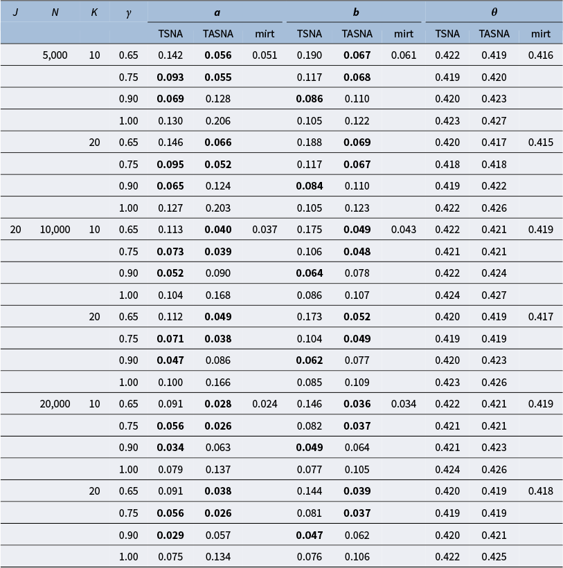

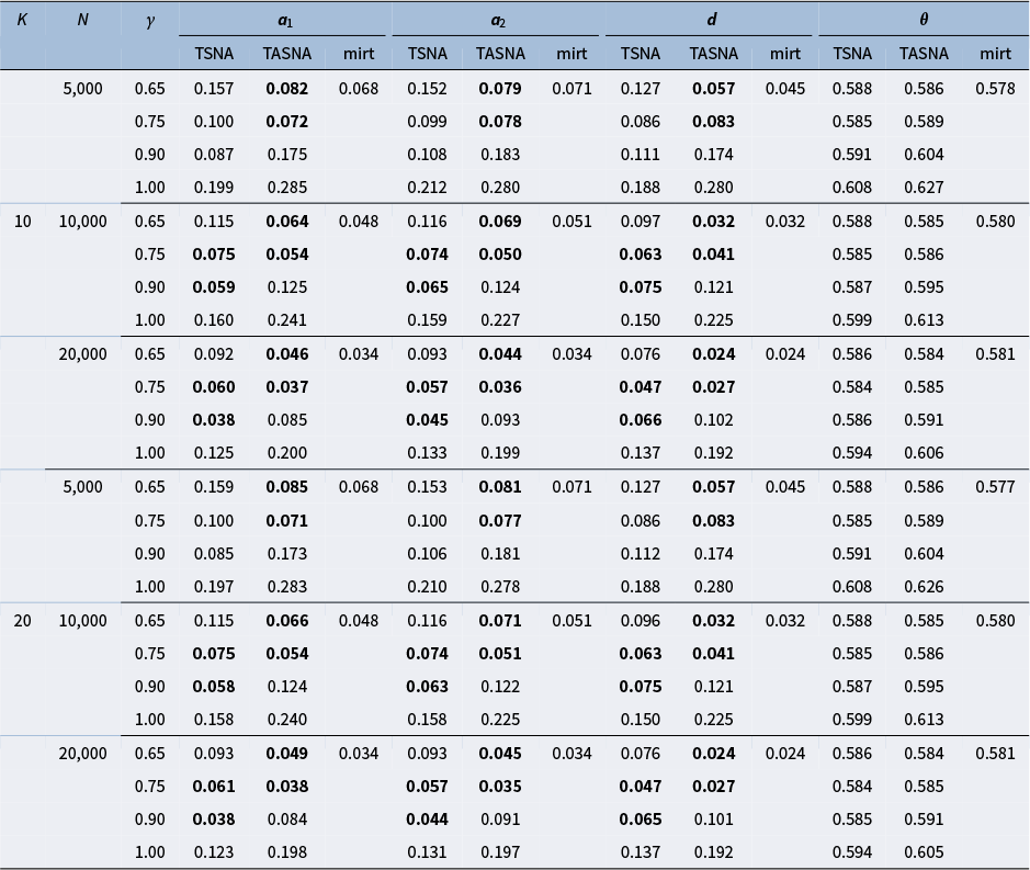


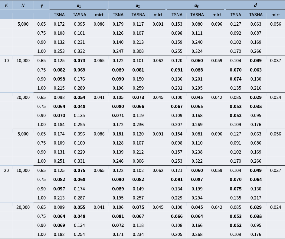


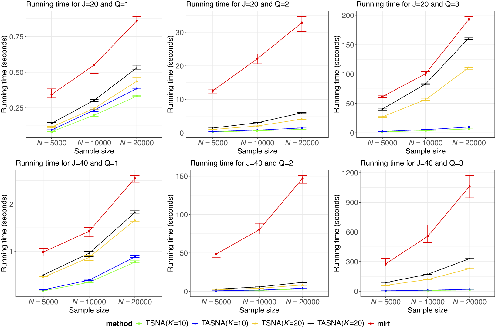
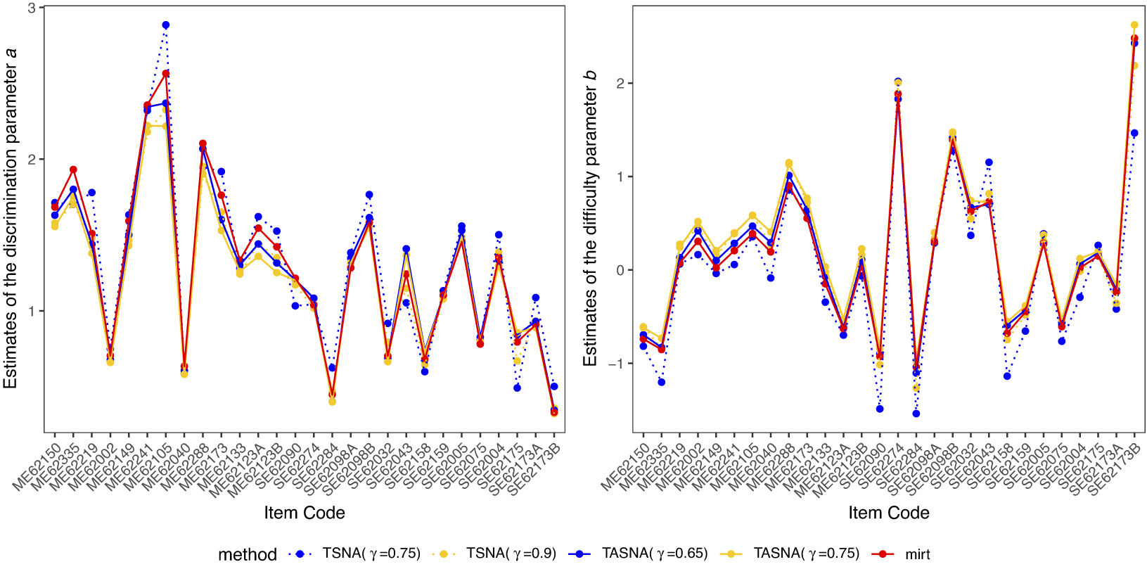


 Open access